transfer learning for predictive models in moocs · transfer learning for predictive models in...

Transfer Learning for Predictive Models in MOOCs

by

Sebastien BoyerDiplôme d’Ingénieur, Ecole Polytechnique (2014)

Submitted to the Department of Electrical Engineering and ComputerScience and the Institute for Data, Systems, and Society in partial

fulfillment of the requirements for the degrees of

Master of Science in Technology and Policyand

Master of Science in Computer Science

at the

MASSACHUSETTS INSTITUTE OF TECHNOLOGY

June 2016

c○Massachusetts Institute of Technology 2016. All rights reserved.

Author. . . . . . . . . . . . . . . . . . . . . . . . . . . . . . . . . . . . . . . . . . . . . . .May 20, 2016

Certified by . . . . . . . . . . . . . . . . . . . . . . . . . . . . . . . . . . . . . . . . . . .Kalyan Veeramachaneni, Principal Research Scientist

Thesis supervisor

Accepted by . . . . . . . . . . . . . . . . . . . . . . . . . . . . . . . . . . . . . . . . . . .Professor Munther A. Dahleh

Acting Director, Technology and Policy Program

Accepted by . . . . . . . . . . . . . . . . . . . . . . . . . . . . . . . . . . . . . . . . . . .Professor Leslie A. Kolodziejski

Chair, EECS Committee on Graduate Students

1

Transfer learning for predictive models in MOOCs

by

Sebastien Boyer

Submitted to the Institute for Data, Systems, and Society and the Department ofElectrical Engineering and Computer Scienceon May 20, 2016, in partial fulfillment of the

requirements for the degree ofMaster of Science in Technology and Policyand Master of Science in Computer Science

Abstract

Predictive models are crucial in enabling the personalization of student experiencesin Massive Open Online Courses. For successful real-time interventions, these modelsmust be transferableâĂŤ- that is, they must perform well on a new course from adifferent discipline, a different context, or even a different MOOC platform.

In this thesis, we first investigate whether predictive models “transfer” well to newcourses. We then create a framework to evaluate the “transferability” of predictivemodels. We present methods for overcoming the biases introduced by specific coursesinto the models by leveraging a multi-course ensemble of models. Using 5 coursesfrom edX, we show a predictive model that, when tested on a new course, achievedup to a 6% increase in AUCROC across 90 different prediction problems. We thentested this model on 10 courses from Coursera (a different platform) and demonstratethat this model achieves an AUCROC of 0.8 across these courses for the problem ofpredicting dropout one week in advance. Thus, the model “transfers” very well.

Thesis Supervisor: Kalyan VeeramachaneniTitle: Principal Research Scientist, Institute for Data, Systems and Society, CSAIL

3

Acknowledgments

I am very grateful to acknowledge the financial support of the National Science Foun-

dation which funded this research project to explore the future of Massive Open

Online Course education. My gratitude also goes to the teams at edX (which pro-

vided the project with the preliminary data sets) who work every day to provide a

free and high-quality education to students around the globe, and who took the time

to meet and help guide this project along the way.

As I look back on almost two years of studies at MIT, too many people deserve

my most humble and grateful acknowledgments for me to possibly mention them all

here. Kalyan Veeramachaneni, my research advisor, has been a particularly helpful

mentor throughout these two years. First, he has been flexible enough to comply

with my great appetite for classes (leading me to complete two programs). He was

also able to focus my energy when my research interests became too diverse, and he

certainly taught me what scientific exigence and excellence mean. In the lab, I can’t

start explaining how amazed I have been by all the great thoughts my fellow students

had over these few months. From the great theoretical discussions with Sebastien

Dubois to all the engineering ideas exchanged with Benjamin Schreck, I am humbled

by all the insights that I received from them.

In MIT at large, I will simply start by acknowledging the impact that some pro-

fessors had on me through my time here : among them, David Autor, for his timeless

course on Labor Economics, Kenneth Oye for his interesting ideas on the incentives

at play in regulation making processes, and Erik Brynjolfsson for his famous class on

the Digital Economy.

I will always be indebted to the dozens of students at MIT with whom I exchanged,

discussed, debated and worked over these past two years. You are the ones who have

made my experience here at MIT what it truly was : inspiring. To cite only some

of them, I am honored to have met such great people as Nicola Greco and Adam

Yala and I am looking forward to more of our inspiring dinners. I will miss forever

the great people of the Technology and Policy Program. I want to thank everyone

5

of them for their great energy and spirit, that make this program unique. A special

note to my fellow French-citizen, Anne Collin, to have shared my joys, my sweat and

my doubts throughout.

Finally, I want to give a special note to my two partners in crime over those

two years : Maximilien Burq and Sebastien Martin. It has been an amazing and

intellectually very exciting period of my life thanks to your curiosity, ideas and energy,

and I am looking forward to more of our scientific projects, philosophical discussions

and random parties.

I can’t end this page without paying tribute to the support and care of my family

over those two years and more importantly throughout my life. My parents have

always been my models. I value their advices, thoughts and doubts far more than I

like to admit. I will never thank them enough to have raised me in a world where

daring to stand for others is the pillar of a successful life.

I dedicate this thesis to my little sister Tiphaine, whose joy and smile I missed

the most during those two years. Surprisingly, I have never felt closer to her since I

have left my home country to join MIT two years ago.

Finally, I want to express my love, my admiration and my infinite gratitude to

Caroline to make my life just infinitely more interesting and beautiful.

6

Contents

1 Introduction 15

1.1 Challenge of Personalization on MOOCs . . . . . . . . . . . . . . . . 17

1.2 On the use of Predictive Models . . . . . . . . . . . . . . . . . . . . . 19

1.2.1 Current workflow of predictive analytics on MOOCs . . . . . . 20

1.3 Contributions . . . . . . . . . . . . . . . . . . . . . . . . . . . . . . . 22

2 Literature Review 23

2.1 Analytics on MOOCs . . . . . . . . . . . . . . . . . . . . . . . . . . . 23

2.2 Dropout Predictions on MOOCs . . . . . . . . . . . . . . . . . . . . . 24

2.3 Ensembling methods in Performance Prediction . . . . . . . . . . . . 25

3 Data : from sources to features 27

3.1 Data Sets . . . . . . . . . . . . . . . . . . . . . . . . . . . . . . . . . 27

3.2 Behavioral Features . . . . . . . . . . . . . . . . . . . . . . . . . . . . 30

4 Modeling and evaluation 35

4.1 Preliminaries . . . . . . . . . . . . . . . . . . . . . . . . . . . . . . . 35

4.1.1 Definitions . . . . . . . . . . . . . . . . . . . . . . . . . . . . . 35

4.1.2 Evaluation Metric and Algorithms . . . . . . . . . . . . . . . . 38

4.1.3 Baseline models evaluated . . . . . . . . . . . . . . . . . . . . 41

4.1.4 Markov assumption on MOOCs . . . . . . . . . . . . . . . . . 42

4.2 Evaluating models across Courses . . . . . . . . . . . . . . . . . . . . 43

4.2.1 Definition of a simple method : Naive transfer . . . . . . . . . 44

7

4.2.2 Evaluation of Naive transfer . . . . . . . . . . . . . . . . . . . 45

5 Building transferable models 47

5.1 Formalism of ensemble methods . . . . . . . . . . . . . . . . . . . . . 47

5.2 Experiments . . . . . . . . . . . . . . . . . . . . . . . . . . . . . . . . 52

5.2.1 Single course - Multiple algorithms . . . . . . . . . . . . . . . 52

5.2.2 Concatenated course - Multiple algorithms . . . . . . . . . . . 53

5.2.3 Deep Ensembling methods . . . . . . . . . . . . . . . . . . . . 54

5.3 Results . . . . . . . . . . . . . . . . . . . . . . . . . . . . . . . . . . . 56

5.3.1 Single course - Multiple algorithms . . . . . . . . . . . . . . . 56

5.3.2 Concatenated course - Multiple algorithms . . . . . . . . . . . 57

5.3.3 Deep ensembling methods . . . . . . . . . . . . . . . . . . . . 58

5.3.4 Transferring across MOOC platforms . . . . . . . . . . . . . . 59

5.3.5 Releasing a Package for Ensembling Methods . . . . . . . . . . 62

6 Deploying a Dropout Prediction System 67

6.1 Motivation and Deployment Opportunities . . . . . . . . . . . . . . . 67

6.1.1 Partnership with a leading MOOC provider . . . . . . . . . . 67

6.1.2 Purposes of Large Scale Public Deployment . . . . . . . . . . 68

6.2 Challenges of Deploying a Machine Learning Pipeline . . . . . . . . . 70

6.2.1 Translation Step . . . . . . . . . . . . . . . . . . . . . . . . . 70

6.2.2 Extraction Step . . . . . . . . . . . . . . . . . . . . . . . . . . 72

6.2.3 Prediction Step . . . . . . . . . . . . . . . . . . . . . . . . . . 73

6.2.4 Specific Challenges to Dropout Predictions . . . . . . . . . . . 74

6.3 Multi-steps Deployment . . . . . . . . . . . . . . . . . . . . . . . . . 77

6.3.1 Technical Solutions for the Three Steps . . . . . . . . . . . . . 77

6.3.2 MyDropoutPrediction : a Web Platform for Dropout Prediction 79

8

List of Figures

1-1 Number of MOOC courses available in the world. A parabolic interpo-

lation on the monthly evolution yields : 𝑦 = 1.7718𝑥2 − 5.7192𝑥 with

𝑅 = 0.99775. Source : https://www.class-central.com/report/moocs-

2015-stats/ . . . . . . . . . . . . . . . . . . . . . . . . . . . . . . . . 16

1-2 Number of MOOC courses available per platform. Coursera alone

accounts for more than 1497 courses, a percentage of 36% of the total.

Source : https://www.class-central.com/report/moocs-2015-stats/ . . 16

3-1 An event recorded in a MOOC course log file. This event was generated

after a user submitted an answer to problem. . . . . . . . . . . . . . . 28

3-2 Two dimensional cut of the normalized (in the unit hyper-cube)

feature space for the behavioral features of Course 1 on the second

week. (Darker squares refer to higher Average of non-dropout on week

3.) . . . . . . . . . . . . . . . . . . . . . . . . . . . . . . . . . . . . . 34

4-1 Illustration of the (𝑤3, 𝑤6) Dropout Prediction Problem on a 8-week-

long course. . . . . . . . . . . . . . . . . . . . . . . . . . . . . . . . . 37

4-2 List of the four basic classification algorithms used for dropout

prediction along with their parameters and the range over which these

are optimized through 5-fold cross-validation. . . . . . . . . . . . . . 41

4-3 AUC of self-prediction method on the first three courses for different

prediction problems using a Logistic Regression classification algo-

rithm. Each line represent DPP with the same current week (𝑤𝑐), the

x coordinate represent the prediction week . . . . . . . . . . . . . . . 42

9

4-4 AUC improvement over a model built from week 1 for different values

of Lag. Self-prediction method is used on the first three courses. . . . 43

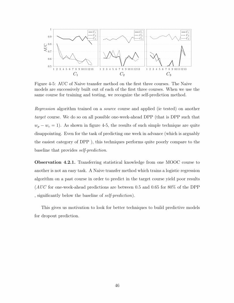
4-5 AUC of Naive transfer method on the first three courses. The Naive

models are successively built out of each of the first three courses.

When we use the same course for training and testing, we recognize

the self-prediction method. . . . . . . . . . . . . . . . . . . . . . . . . 46

5-1 Illustration of two Ensembling structures yielding two different

predictions. For this illustration we use a simple majority merging

rule. Circles represent basic predictors while triangles stand for merge

rules. The colors indicate a binary the prediction. . . . . . . . . . . 51

5-2 Example of an ensembling structure for dropout prediction based on

two source courses and three different classification algorithms. . . . . 52

5-3 Illustration of the six Ensembling Methods structures compared when

used with three source courses and three algorithms. . . . . . . . . . 55

5-4 Performance on target course 𝐶0 of the different “Single course”

methods to build predictive models. Displayed is the average (standard

deviation) of the DAUC over all possible DPP (less is better). . . . . 57

5-5 Performance on target course 𝐶0 of the different “Single course”

methods as well as the “Concatenaed” method. Displayed is the

average (standard deviation) of the DAUC over all possible DPP (less

is better). . . . . . . . . . . . . . . . . . . . . . . . . . . . . . . . . . 58

5-6 Average (standard deviation) DAUC of different structures. 𝐷𝑃𝑃

refers to all Dropout Prediction Problems common to the five courses

while 𝐷𝑃𝑃𝑠ℎ𝑜𝑟𝑡 refers to one-week-ahead Dropout Prediction Problems

only. . . . . . . . . . . . . . . . . . . . . . . . . . . . . . . . . . . . . 60

5-7 Average DAUC over all short prediction problems on the 10 Coursera

courses taken as target (only edX courses are taken as source courses). 61

5-8 AUC achieved by 𝑆2 ensembling method built on the five edX courses

and applied on the 10 Coursera courses. . . . . . . . . . . . . . . . . 61

10

5-9 Code snippet 1/3 of a simple utilization of Deep ensembling. . . . . . 64



6-1 Three independent steps of the Dropout Prediction Process . . . . . . 71

6-2 List of tables populated in the MySQL database by the "Translation

step". . . . . . . . . . . . . . . . . . . . . . . . . . . . . . . . . . . . 71

6-3 Illustration of the extraction of a feature ("Number of feature watched

per week") from a structure database and a feature-defining script. . 73

6-4 Sharing machine learning models through a web-browser separate the

need to share data with the service provider. . . . . . . . . . . . . . 80

6-5 Example of use case on 𝑀𝑦𝐷𝑟𝑜𝑝𝑜𝑢𝑡𝑃𝑟𝑒𝑑𝑖𝑐𝑡𝑖𝑜𝑛 web application. . . 82

6-6 Definition of the three sets of features that users can use on My-

DropoutPrediction web application. The Features labels refer to table

3.2 . . . . . . . . . . . . . . . . . . . . . . . . . . . . . . . . . . . . . 82

11

List of Tables

3.1 Details about the 16 Massive Open Online Courses from MIT offered

via edX and Coursera platforms. The courses span over a period of

3 years and have a total of 271,933 students. * Students represented

here are students who are present in the log files, which is the students

who perform at least one interaction with the interface (video played,

problem attempted, ...). . . . . . . . . . . . . . . . . . . . . . . . . . 29

3.2 Features extracted from the log-files and used to predict dropout . . . 31

3.3 Basic statistics of the features extracted for Course 1 and week 2 . . . 32

13

Chapter 1

Introduction

Since their creation in 2012, Massive Open Online Course platforms (MOOCs) have

grown dramatically in terms of both number and reach. From 2014 to 2015, the

number of MOOC students doubled 1, eventually reaching 35 million unique students.

Figure 1-1 summarizes the growth in course offerings across the globe over the past

four years.

More recently, public and private universities have joined independent organiza-

tions like Coursera and edX in the MOOC ecosystem. Some of these schools have

begun offering official degrees upon completion of online courses only 2. Such growth

provides an opportunity to dramatically lower the cost of education, and thus provide

high-quality education to more young people than ever before. As the number of both

courses and students increases, the major platforms have maintained their relative

popularity. In 2015 as in 2014, the main player (Coursera) accounted for about half

of the total number of students and for a third of the total number of courses offered

by all platforms combined, as shown in Figure 1 .

1https://www.class-central.com/report/moocs-2015-stats/2http://news.mit.edu/2015/online-supply-chain-management-masters-mitx-micromasters-1007

15

2012 2013 2014 2015 20160

1,000

2,000

3,000

4,000

Num

ber

ofM

OO

Cco

urse

s

Figure 1-1: Number of MOOC courses available in the world. A parabolic interpo-lation on the monthly evolution yields : 𝑦 = 1.7718𝑥2 − 5.7192𝑥 with 𝑅 = 0.99775.Source : https://www.class-central.com/report/moocs-2015-stats/

020

040

060

080

01,00

01,20

01,40

01,60

0

CourseraedX

CanvasFutureLearn

OthersMiroada

France University NumeriqueUdacity

Open EducationRwaq

IversityNovoEd

Number of MOOC courses

Figure 1-2: Number of MOOC courses available per platform. Coursera alone ac-counts for more than 1497 courses, a percentage of 36% of the total.Source : https://www.class-central.com/report/moocs-2015-stats/

16

1.1 Challenge of Personalization on MOOCs

Despite the promises of MOOCs, concerns remain about their ability to provide a

quality alternative to traditional education. One big question emerges from MOOCs’

lack of personalization.

The personalization gap: Most teachers in traditional classrooms have direct con-

tact with students. This access enables them to take two kinds of action: First, it

helps them to gather specific information about students (“How is Annah doing in

the class ?”,“How much homework did she complete?”,“How are her grades compared

to other students?”), and second, it allows them to adapt and personalize the content

and/or format of the class to specific needs (“Annah will benefit from these additional

resources about this topic she didn’t quite get”,“Tom should probably put more effort

into his homework in order to learn the content”). Addressing and adapting to each

student’s unique needs is arguably one of the most important aspects of education

[26], [3].

MOOCs differ from traditional education in a major way: a far higher student-

teacher ratio. Single courses may have 40, 000 or more students, making it difficult

for teachers (or the teaching team) to assess, reach out to, and interact with stu-

dents individually. This has become a major concern within the MOOC education

community [13],[3].

MOOCs also suffer from a low completion rate 3. MOOC completion rates are

almost always under 10% - far lower than those of traditional degree programs. There

are many and diverse reasons for this, as shown in [16], but personalization is a major

one. With so much rich data available, it is natural to ask whether we can leverage

this particular strength of MOOCs to personalize the experience, and help improve

completion rates.

The promise of data: The growing reach of MOOC courses provides the opportu-

3number of students successfully completing the minimum requirements to earn the certificate,divided by the number of student who enrolled in the course

17

nity to work with an unprecedented amount of student data 4. Not only do MOOCs

provide two types of meaningful student-related data (personal information about

who the student is, and behavioral information about what the student does), they

allow us to gather this data for students across the globe 5.

When education is studied as a scientific field, whether it is to identify the best

“teaching” strategies or to give students advice about how to learn better, the lack

of experimental data has always posed a major hurdle. Due to the high costs of

gathering relevant data, there are a limited amount of data-based analyses in the

research literature. Between their digital format and the large sample they provide,

MOOC platforms offer a unique opportunity to collect and study information about

the student experience, and to adapt the delivery of pedagogy .

Data-driven approaches to personalization: A data-driven approach to address-

ing personalization is usually structured in five steps:

1. Use past observations to build a predictive model for possible behavioral out-

comes.

2. Posit and design an intervention that is likely to deliver positive outcomes.

3. Use this model to produce predictions regarding a student in real time.

4. Use these predictions to design and execute an intervention.

5. Evaluate whether this intervention improved outcomes.

Initial research aimed toward MOOC personalization mostly focuses on step 16. That is, researchers focus on building predictive models and evaluating them.

Arguably, this is a foundational step in designing an intervention (if intervention is

based on predictions, one has to first evaluate if we are able to predict).4Nowadays, as user data sits at the heart of the main business models of the tech industry, we

as a society have gained tremendous experience in how to record, store and process data.5Every country is represented by MOOCs’ students according to

https://next.ft.com/content/8a81f66e-9979-11e3-b3a2-00144feab7de6For instance, some researchers have tried to predict when and how instructors are likely to

intervene in MOOC forums, but have not undertaken real-life experiments.

18

This approach has been popular because it provides an easy and scalable solu-

tion to adapt traditional teacher intervention behavior for a MOOC context. In

[9], Chaturvedi et al. use an unsupervised learning framework to jointly learn forum

thread topics and the likelihood for instructor to intervene in the thread. In [8], Chan-

drasekaran et al. took another approach: after manually annotating a large corpus of

forum posts, they used a supervised approach and Natural Language Processing to

predict whether an instructor should intervene in a particular thread (that is, they

trained a binary classifier to distinguish between forum threads in which instructors

will intervene, and those that don’t inspire intervention 7). Both works used a classic

validation approach on past data, staying within the context of step 1 as described

above. Though promising, these techniques have not yet led to real-life experiments.

Only one project has successfully tackled all five steps thus farâĂŤin 2015, a

Harvard research group used dropout prediction to target surveys to students during

the course [28]. They identified students “at risk” of dropping out and send them an

email to ask about their lack of engagement. Surprisingly, this survey motivated some

students to re-engage in the class, 8 and increased the comeback rate of the survey

receivers to up to 1% (with a p-value of 0.02) in certain cases.

1.2 On the use of Predictive Models

As we mentioned, using a data-driven approach to improve MOOC personalization

involves a five-step process. This procedure brings with it an oft-underestimated

challenge: the “context" where the predictive model is applied often changes when

going from past data (on which the models are built) to real time. It is hoped that

predictive models which are trained and evaluated on one course will perform the

same on the other course.

In the context of MOOCs, all real-life use cases require us to be able to give

7One major unstated assumption to go from such model to intervention is that the examplesused to train the models are actually “successfull” intervention that we want to reproduce or just“false alarms”

8One of the student responded back : “I was not allocating time for edX, but receiving yoursurvey e-mail recaptured my attention.”

19

predictions on a new (and therefore unseen) course. We illustrate possible differences

between MOOC courses by comparing 6002x, given on edX in September 2012, and

Critical Thinking, given on Coursera in January 2015. These courses differ from one

another with respect to:

∙ Course Content. In addition to covering very different topics, the two courses

contain disparate amounts of content. The first spanned a 14-week period, while

the second was only 5 weeks long.

∙ Student Cohort. The edX course drew a cohort about five times as big as

Coursera’s (51,394 vs. 11,761). It is unclear whether students who enrolled

in 6002x even behave similarly (on average) to the students who enrolled in

Critical Thinking.

∙ Environment. Lastly, the courses were hosted on different platforms and at

different points in time.

One key uncertainty when building predictive models on MOOCs is the question

of "transferability". We say that a predictive model is "transferable" if, after being

trained on a particular course (or, more likely, a set of courses), it performs equally

well on a new, unseen course. This notion, which naturally emerges in the context of

predictive models on MOOCs, is the main focus of this work.

1.2.1 Current workflow of predictive analytics on MOOCs

Despite the potential implications of such work, little attention has been paid so far to

the "transferability" of predictive models across MOOC courses. This is likely due to

the difficulty of gathering enough (and diverse enough) data to study such problems.

Apart from one real-life intervention project [28], most research studies about

predictive analytics on MOOCs have focused on training models on a single course,

or on a restricted set of similar courses. For instance, in [17], Kloft et al. used a

single course to build both their train and their test set. That is, their evaluation

metric was computed on the same course as the one used to learn the parameters of

20

the models. If this strategy often provides good intuition about models, it generally

isn’t a good warranty of performance on other courses. In [9], Chaturvedi et al.

trained their intervention recommendation system on data from two Coursera courses.

This workflow is typical of most published work on MOOC analytics, and can be

summarized in the five following steps :

1. Define a prediction problem.

2. Divide data for a single course into a training set and a testing set.

3. Learn a model on the training set.

4. Tune the model parameters using cross-validation on the training set.

5. Report the model’s accuracy on the test set.

To the best of our knowledge, only Halawa et al. in [15] and Boyer et al. in [5]

and [4] reported results for models trained on a set of courses different from the set

used for testing. This provided a first step toward greater reliability of the reported

accuracy (Halawa et al. used six courses for training and reported average results on

ten unseen courses). In the work that follows, we offer a new framework to build and

test predictive models on MOOCs. We argue that our framework enables researchers

to report “test” performances that are closer to real life, thus bridging the gap between

in-house and real life performances. Our framework, which will be described in greater

detail later, can be briefly summarized as follows:

1. Define a prediction problem.

2. Take some courses out of the set of available courses and consider these “target

courses,” while all others are “source courses”.

3. Learn a model using all the “source courses”.

4. Tune parameters using cross-validation on the courses. That is, use one of the

“source courses” to test a model, repeat successively over all remaining “source

21

courses,” and choose the model that leads to the best averaged performance

over these iterations.

5. Report the model’s average accuracy over all “target sources” previously unseen

by the algorithms.

1.3 Contributions

Building on these remarks, this work explains in details the challenges, successful

methods, and results pertaining to each of the five steps. Concretely, we:

∙ Formally setup a framework to evaluate “transferability” of predictive models

on MOOCs.

∙ Create a structured approach to use ensembling methods as a way to leverage

data from diverse sources in order to build models that “transfer” well to new

courses.

∙ Give quantitative results describing how different predictive models “transfer”

to new courses.

∙ Find a predictive model for dropout prediction that successfully “transfer” to

new courses both from the same and from different MOOC platforms.

∙ Discuss requirement and challenges associated with deploying a public solution

for dropout prediction.

∙ Provide a complete software solution to go from raw log files from a MOOC

platform, to the dropout predictions for the students of that platform.

These contributions go along with thorough discussion of the challenges of “trans-

fering” predictive models on MOOCs both from a theoretical and a practical perspec-

tive. Our high-level goal through this work is to give a significant contribution to

help close the “personalization gap” on MOOCs.

22

Chapter 2

Literature Review

Because of these transforming promises for education research, MOOCs have been a

particularly attracting research field from their creation onward. Particular interest

have been focused on the possibility to use data from MOOCs to inform learning

theory, and to study the reasons behind the surprisingly low completion rates. Un-

surprisingly, analytics research papers have flourished about MOOCs in general, and

around the problem of predicting student dropout in particular.

In this section, we explore some past attempts to leverage MOOC data to perform

analytics and to predict dropout, and highlight more recent literature around using

a particular machine learning method to improve prediction accuracy in the context

of MOOCs.

2.1 Analytics on MOOCs

In 2012, MOOCs began to emerge from a growing online learning community. This

community had started to motivate research about the challenges and opportunities

of new types of education.

In 2007, Allen et al. described the state of online learning in US higher education [1].

They focused on identifying the barriers preventing wide adoption of online learning

by universities. Among their top barriers were online students’ lack of discipline, and

lower retention rate.

23

Online learning has been described as an "inflection point" in the availability

of educational data, which is very difficult to gather in more traditional classroom

settings [19], [2].

More than innovative devices or classroom designs, big data and analytics have been

identified as the most promising tools of future education [25]. The authors of [25]

see "the availability of real-time insight into the performance of learners" as one of

the most important contributions of online learning.

In 2012, following the growth of research interest in using analytics to improve and

learn from online courses, the authors of [24] presented a holistic vision to advance

"Learning Analytics" as a research discipline. In [14], Ferguson et al. also present a

brief history of the field, as well as its differences from other related technical fields

such as data mining and academic analytics.

2.2 Dropout Predictions on MOOCs

Even before the recent e-learning boom, concerned researchers attempted to predict

dropout. One major obstacle facing such attempts is the difficulty of building robust

predictive algorithms. While working with early e-learning data, the authors of [20]

improved the performance of their learning algorithm by merging several predictive

algorithms together, namely Support Vector Machines, Neural Networks, and Boosted

Trees.

Since then, almost all dropout studies have been conducted on MOOC data. Some

researchers (like the authors of [22], who studied the effects of collaboration on the

dropout rate of students) focus on understanding the drivers of dropout among stu-

dents. Others develop feature extraction processes and algorithms capable of pin-

pointing at-risk students before they drop out. If a MOOC is able to identify such

students early enough, these researchers reason, it may be possible for educators to

intervene. In [15], Halawa et. al. used basic activity features and respective per-

formance comparison to predict dropout one week in advance. The authors of [4]

included more features, as well as an integrated framework that allowed users to

24

apply these predictive techniques to MOOC courses from various eligible platforms.

As MOOC offerings proliferate, the ability to "transfer" statistical knowledge

between courses is increasingly crucial, especially if one wants to predict dropout in

real time. Unfortunately, it is often difficult to take models built on past courses and

apply them to new ones. In [5], Boyer and Veeramachaneni showed that models built

on past courses don’t always yield good predictive performance when applied to new

courses.

2.3 Ensembling methods in Performance Prediction

Since competition-based analytics emerged in 2010, the appetite for more complex and

accurate predictive models has increased. Ensembling, a machine learning technique

that combines several predictive models, has been explored as one way to improve

the performance of predictive models in education.

Over the past twenty years, a flourishing predictive literature has appeared, of-

fering various techniques for choosing and ensembling models in order to achieve

high-performing predictors. A technique called "stacking" has proven particularly

promising. In [12], Svzeroski et. al. showed that stacking models usually perform as

well as the best classifiers. They also confirmed that linear regression is well-suited

to learning the metamodel, and introduced a novel approach based on tree models.

The authors of [7] demonstrated the possibility of incrementally adding models to

the "ensembling base" from a pool of thousands. Sakkis et. al. [23] used the stack-

ing method to solve spam filtering problems, finding that it significantly improved

performance over the benchmark.

The authors of [18] explored using ensembling methods to combine several "in-

cremental statistical models," in order to predict student performance in the context

of distance education. They found that ensembling methods successfully improved

on the best of these individual models. In the same year, 2010, the authors of [29]

won the KDD-cup competition, which focuses on predicting the future performance of

real-life students based on their past behavior. A combination of feature engineering

25

and ensembling methods resulted in the most accurate classifiers. In [10], building

on the observation that past research was split on which models to use for predict-

ing dropout, Baker et al. proposed using ensembling methods across these models.

They used an "Intelligent Tutoring System" to track students’ behavior and perfor-

mance, and found mixed results depending on the metric used to evaluate student

performance (online vs. paper test).

Remarking that these two papers led to contradictory conclusions about ensem-

bling methods (success for the former, mixed results for the latter), the authors of [21]

used a different tutoring system ("ASSISTments Platform") to gather more student

data and re-evaluate the methods’ performance. After exploring up to eight models

and eight ensembling methods, the authors found an improvement of 10% over the

best individual predictive model.

In this paper, we explore a framework for building robust predictive models ap-

plicable to MOOCs. Although we do address dropout prediction specifically, we also

consider the broader possibilities for building predictive models from a set of courses.

In particular, we offer ensembling methods that mix predictive models built on dif-

ferent data sources, which, to the best of our knowledge, has never been tried before

in the context of student performance prediction.

26

Chapter 3

Data : from sources to features

In order to provide a convincing approach for the study of “transferability” across

MOOCs, we based our work on several courses’ worth of data. In the next chapter,

we use this data to build and test our framework for transferring predictive models

across courses. In this chapter, we focus on a few preliminary questions: which data

to use, where to find it, and how to use it.

3.1 Data Sets

Different data streams on MOOCs Like other digital user interfaces, MOOC

platforms (both websites and apps) record and store detailed information about their

users. For MOOC students, this rich data can be decomposed into three main streams

:

∙ Demographic information, such as students’ sex, social status, interest in

the course, etc.

∙ Interaction information between users and the interface. This is captured

through clicks or taps made by the users on the platforms.

∙ Forum posts on the course website. These are the comments, questions or

other textual information that students put on the course’s forum page.

27

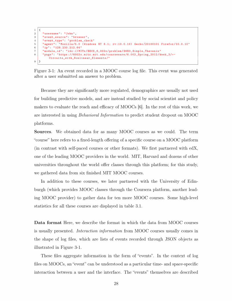
1 {

2 "username": "John",

3 "event_source": "browser",

4 "event_type": "problem_check"

5 "agent": "Mozilla /5.0 (Windows NT 6.1; rv :10.0.10) Gecko /20100101 Firefox /10.0.10"

6 "ip": "128.230.212.64"

7 "module_id": "i4x:// MITx/EECS_6_002x/problem/S6E0_Simple_Thevenin"

8 "page": "https ://6002x.mitx.mit.edu/courseware /6.002 _Spring_2012/Week_3/←↩Circuits_with_Nonlinear_Elements/"

9 }

Figure 3-1: An event recorded in a MOOC course log file. This event was generatedafter a user submitted an answer to problem.

Because they are significantly more regulated, demographics are usually not used

for building predictive models, and are instead studied by social scientist and policy

makers to evaluate the reach and efficacy of MOOCs [6]. In the rest of this work, we

are interested in using Behavioral Information to predict student dropout on MOOC

platforms.

Sources. We obtained data for as many MOOC courses as we could. The term

“course” here refers to a fixed-length offering of a specific course on a MOOC platform

(in contrast with self-paced courses or other formats). We first partnered with edX,

one of the leading MOOC providers in the world. MIT, Harvard and dozens of other

universities throughout the world offer classes through this platform; for this study,

we gathered data from six finished MIT MOOC courses.

In addition to these courses, we later partnered with the University of Edin-

burgh (which provides MOOC classes through the Coursera platform, another lead-

ing MOOC provider) to gather data for ten more MOOC courses. Some high-level

statistics for all these courses are displayed in table 3.1.

Data format Here, we describe the format in which the data from MOOC courses

is usually presented. Interaction information from MOOC courses usually comes in

the shape of log files, which are lists of events recorded through JSON objects as

illustrated in Figure 3-1.

These files aggregate information in the form of “events”. In the context of log

files on MOOCs, an “event” can be understood as a particular time- and space-specific

interaction between a user and the interface. The “events” themselves are described

28

Course Platform Start Date Weeks Students* Name

6002x edX 2012/05/09 14 51,394 𝐶0

3091x edX 2012/09/10 12 24,493 𝐶1

3091x edX 2013/05/02 14 12,276 𝐶2

1473x edX 2012/12/02 13 39,759 𝐶3

6002x edX 2013/03/03 14 29,050 𝐶4

201x edX 2013/04/15 9 12,243 𝐶5

aiplan-001 Coursera 2013/01/28 5 9,010 𝐶6



animal-001 Coursera 2014/07/14 5 8,577 𝐶9

animal-002 Coursera 2015/02/09 5 5,431 𝐶10

astrotech-001 Coursera 2014/04/28 6 6,251 𝐶11codeyourself-001 Coursera 2015/03/09 7 9,338 𝐶12

criticalthinking-001 Coursera 2013/01/28 5 24,707 𝐶13



Table 3.1: Details about the 16 Massive Open Online Courses from MIT offered viaedX and Coursera platforms. The courses span over a period of 3 years and have atotal of 271,933 students. * Students represented here are students who are presentin the log files, which is the students who perform at least one interaction with theinterface (video played, problem attempted, ...).

29

by a handful of attributes related to the user (e.g. IP address, time), the specific

content on the interface with which she interacted (e.g. video, book, forum,) and

some potential outcomes of the events (e.g. a url link or a grade).

In Figure 3-1, we display a single event taken from a MOOC log file. We see the

user-specific data, along with the field referring to the interface and the type of action

performed.

In their current shape, these do not represent interpretable student behaviorsâĂŤthey

are simply discrete events in space and time. To interpret behavior, we extract higher-

level representation through a process called feature engineering [27].

3.2 Behavioral Features

In Table 3.2, we describe the features extracted from the log files. These features

were defined by both expert and non-expert humans, and are now extracted as part

of a software framework, which we discuss in further detail in the last chapter of

this thesis. (For a thorough description of these features and the process with which

they have been chosen, refer to [27].) These features are typically extracted on a

per-student, per-week basis.

Course specific versus general features According to the general definition cited

above, nothing prevents a feature from being course-specific. Some features given

in [27] are not likely to be extracted from all MOOC courses, because they rely on

information specific to certain types of MOOCs. For instance, the “lab grade” feature

couldn’t be extracted in courses not containing any “lab” environment.

Motivated by our desired to study “transferability” of models across courses, we

specifically removed these features so that our set relies on information likely to be

found in most MOOC courses.

Statistics of extracted features In order to get a better idea of what the extracted

features look like, we display some of the basic statistics of a particular MOOC course

(𝐶0) in Table 3.3.

One early observation is that the distributions of most of the features extracted

30

Label Description1 Whether the student has stopped out or not2 Total time spent on platform3 Number of distinct problems attempted4 Number of submissions5 Number of distinct correct problems6 Average number of submissions per problem7 Ratio of 2 and 58 Ratio of 3 and 59 Average time to solve problems

10 Variance of events timestamp11 Duration of longest observed event12 Total time spent on wiki resources13 Increase in 6 compared to previous week.14 Increase in 7 compared to previous week.15 Increase in 8 compared to previous week.16 Increase in 9 compared to previous week.17 Percentile of 618 Percent of max of 6 over students19 Number of correct submissions20 Percentage of the total submissions that were correct21 Average time between a problem submission and problem due date

Table 3.2: Features extracted from the log-files and used to predict dropout

31

Label Units Mean Std Min Q(25) Median Q(75) Max2 sec 8138 13036 0 0 2526 10994 1366483 unit 18 26 0 0 6 26 1474 unit 20 28 0 0 7 29 1875 unit 8 14 0 0 2 11 1246 unit 1 2 0 0 1 1 527 none 883 2045 0 0 221 997 426198 none 1.76 3.21 0.00 0.00 1.20 2.30 89.009 sec 6712 43779 0 0 0 5 599881

10 sec 5721 8444 0 0 391 9877 4275111 sec 1160 1219 0 0 698 2228 360012 sec 203 722 0 0 0 0 1457313 % 0.34 1.29 0.00 0.00 0.00 0.34 52.0014 % 0.72 3.67 0.00 0.00 0.00 0.14 192.2715 % 0.44 1.11 0.00 0.00 0.00 0.32 18.3316 % 1459 50508 0 0 0 0 317455917 % 28 32 0 0 23 56 10018 % 0.02 0.03 0.00 0.00 0.02 0.02 1.0019 unit 10 16 0 0 3 14 12920 % 0.28 0.30 0.00 0.00 0.20 0.53 1.0021 sec 174176 196784 0 0 102008 334334 604122

Table 3.3: Basic statistics of the features extracted for Course 1 and week 2

32

are skewed toward zero. This can be explained by the fact that many features are

counted as rare events (submissions, problems correct, ...) which yield a lot of zero

values among the population (for example, in any given week, many students won’t

submit any problems, some will submit 1, and very few will submit more than 1).

A second remark is that these behavioral features often significantly influence the

outcome at stake (dropout). Table 3-2 shows two 2𝐷-cut of the high-dimensional

space containing the student’s data. To create this table, we proceed as follows:

∙ For each student of course 𝐶0, we extract two behavioral features on week 2.

∙ We group the students into bins in the 2𝐷 space corresponding to these two

behavioral features.

∙ For each bin, we count the number of students who remain in the class (no-

dropout) on week 3, and we divid this number by the total number of students

in that bin.

∙ We color the bin according to this number, so that the darker the bin, the higher

the percentage of that bin’s students still remaining on week 3.

We observe that the percentage of dropout varies significantly from one point of

the plane to another. The fact that we can clearly observe regions of darker squares

gives us hope that we can try to use these features in order to estimate the dropout

status of a student.

Finally, thanks to table 3-2, we remark that the subspace of dropout students

can be easily distinguished from that of non-dropout students simply by observing

the data (through some threshold, for example). As in most data science problems,

the two classes that we hope to predict for students (dropout or non-dropout) are

neither linear nor perfectly separable. The techniques we discuss in the next chapter

all aim at finding accurate ways to "draw a line between", "distinguish between", or

"properly categorize" dropout and non-dropout students.

33

(a) X-axis : 4 | Y-axis : 17 (b) X-axis : 11 | Y-axis : 12

Figure 3-2: Two dimensional cut of the normalized (in the unit hyper-cube) featurespace for the behavioral features of Course 1 on the second week. (Darker squaresrefer to higher Average of non-dropout on week 3.)

34

Chapter 4

Modeling and evaluation

In this chapter we present our contribution : a framework to design and evaluate

predictive models. We start by formally introducing dropout predictions along with

some general choices (such as the choice of a metric to compare predictive models). We

then describe how we can leverage data from different past courses to build predictive

models and evaluate on a new course.

4.1 Preliminaries

In this section we introduce the formal notations and definitions that we use to define

the dropout prediction challenge.

4.1.1 Definitions

To set a format framework to discuss dropout prediction, we need to explain what

we defined as a MOOC course and what it is to dropout a course. This will led us to

define a dropout prediction problem on which “predictors” can use “variables” about

the students’ behavior to predict their dropout.

MOOC Course. The first entity that we use in the discussion below is a course.

Here by course we refer to a fixed-length offering of a particular MOOC course.

While there are on-demand classes that certain MOOC platform offer, we restrict

35

our discussion to course that require students to start at a particular date and to

follow a given schedule. At the time of writing, the typical duration of these courses

vary between five and fourteen weeks. Dropout is defined as a state of students as

described below :

Definition 4.1.1. Dropout. For a student 𝑠 and a point 𝑤, we will say that 𝑠 “has

dropped out” at time 𝑤 if 𝑠 does not submit any assignment after time 𝑤. We model

this unknown binary information as a Bernoulli random variable (whose value is 0 if

the student is dropped out) :

At time 𝑤, for student 𝑠 : 𝑦𝑤𝑠 ∈ {0, 1} (4.1)

We remark that given the above definition of dropout, if a student has dropout

at time 𝑤 she will always be dropout for any 𝑤′ > 𝑤.

We next choose to discretize time so that the range of values taken by 𝑤 is now

finite. Specifically an appropriate time step used in the literature on dropout predic-

tion is 7 days. This time scale it typically chosen because it offers a good balance

between interpretability of the predictive models and simplicity of the computation

used to build them. For a given course 𝐶 we will denote by 𝑊𝐶 the set of weeks over

which 𝐶 spans.

Definition 4.1.2. Dropout Prediction Problem (DPP). We call DPP (𝑤𝑐, 𝑤𝑝)

the task to identify which of the students present in the class at week 𝑤𝑐 will be

dropped out on week 𝑤𝑝 (the students dropping out between week 𝑤𝑐 and week 𝑤𝑝).

We define what we call a Dropout Prediction Problem (that is a prediction task that

is possible to perform on a course) below, and remark that given a particular course

𝐶, there exist exactly 𝑊𝐶 .(𝑊𝐶−1)2

potential problems of this type (that is because each

unique couple (𝑤𝑐, 𝑤𝑝) ∈ {1, ...,𝑊𝐶} such that 𝑤𝑐 < 𝑤𝑝 define exactly one prediction

problem).

We remark that the definition of DPP doesn’t consider students already dropout

at week 𝑤𝑐 (for which the outcome at week 𝑤𝑝 is obvious based on the definition of

dropout).

36

w3 w6

Start End

Figure 4-1: Illustration of the (𝑤3, 𝑤6) Dropout Prediction Problem on a 8-week-long course.

Definition 4.1.3. One-week-ahead DPP . We call One-week-ahead dropout pre-

diction problem a DPP (𝑤𝑐, 𝑤𝑝) such that 𝑤𝑐 = 𝑤𝑝 − 1.

Variables. Given a course 𝐶 we assume to have access to a set of variables

𝑥𝑤𝑠 , 𝑤 ∈ 𝑊𝐶 (for all students 𝑠 of 𝐶) describing their behavior. These variables are

described in Chapter 3 and their number may vary depending on the information

available for each particular course. We have set of behavioral features available,

thus:

∀𝑠 ∈ 𝐶, ∀𝑤 ∈ 𝑊𝐶 , 𝑥𝑤𝑠 ∈ R|𝐹 | (4.2)

Given a particular DPP (𝑤𝑐, 𝑤𝑝), our goal is to use a subset of features 𝑥𝑤𝑠 in 4.2 for

𝑤 up until 𝑤𝑐 to estimate the following quantities

∀𝑠 ∈ 𝐶, 𝑦𝑤𝑝𝑠 (4.3)

Predictors. In order to make predictions on a particular DPP, we build statistical

models (also called predictive models) on a set of students for which we try to capture

the statistical relationship between features {𝑥𝑤𝑐𝑠 , 𝑤 ∈ 𝑊𝐶} and outcome 𝑦𝑤𝑝 .

Definition 4.1.4. Predictor. We call predictor for the DPP (𝑤𝑐, 𝑤𝑝) and the set of

feature 𝐹 , a function 𝜑𝑤𝑐,𝑤𝑝 : 𝑅|𝐹 |x|𝑁𝑤| → [0, 1] (where 𝑁𝑤 is the number of weeks

effectively taken into account by the statistical model). We call predictions of 𝜑𝑤𝑐,𝑤𝑝

for course 𝐶 the following quantities

∀𝑠 ∈ 𝐶, 𝜑𝑤𝑝,𝑤𝑐({𝑥𝑤𝑐𝑠 , 𝑤 ∈ 𝑊𝐶}) (4.4)

37

Predictors are usually learned on features extracted before week 𝑤𝑐 and outcomes

extracted on week 𝑤𝑝. A good predictor is one such that 𝜑𝑤𝑐,𝑤𝑝({𝑥𝑤𝑐𝑠 , 𝑤 ∈ 𝑊𝐶}) is

"close" to 𝑦𝑤𝑝𝑠 . How to define “close” and how to measure it on various DPP for

various courses is the topic of the next section.

4.1.2 Evaluation Metric and Algorithms

In order to evaluate different predictive models we need to account for the variance

of the different courses and the different DPPs. Certain technique might perform

better on a particular course or for a particular DPP. On the other hand, we are

interested in discovering a framework to learn predictive models both applicable in

real-life settings and easily repeatable which adds to the complexity of the choice of

a metric.

Choice of a basic metric. Since this metric will be usually taken as the optimization

objective, different metric choices will yield different final algorithms. In our case,

a classification problem, the easiest metric that come to mind is the accuracy (as

defined below). Two difficulties with optimizing for accuracy however arise when

dealing with unbalanced data sets.

Definition 4.1.5. Accuracy Ratio between the number of correctly categorized

samples over the total number of samples. This value depends not only on the pre-

dictive model but also on the threshold value chosen to express our preference over

the cost of false positive predictions versus the cost of false negative predictions.

First the accuracy level will highly depend on the balance between classes (if

one class accounts for almost 100% of the samples, then a simple method predicting

always this class will yield very high accuracy). Secondly, measuring the accuracy

implicitly makes us assume a fixed ratio between how much we value a false positive

mistake and how much we value a false negative. In real-life use cases, this is often

not the case and this ratio depends a lot on the different applications and how the

user choose to use the predictive model. We therefore need to find a metric better

38

suited to our problem 1.

In order to overcome both concerns about the above metric, we choose the Area

Under the Receiver Operating Characteristic curve. We will refer to this metric as

AUC .

Definition 4.1.6. AUC Area under the curve of the Receiver Operating Char-

acteristic curve. Where the "Receiver Operating Characteristic" curve is the curve

defined by all the values of the tuple (True positive, False Positive) when varying the

"positive" threshold from 0 to 1 on the predicted probability to belong to the positive

class. We call 𝐴𝑈𝐶𝑝𝑚 the AUC of model 𝑚 on the prediction problem 𝑝.

A probabilistic interpretation of the AUC is the following : "Given a positive and

a negative example, the AUC of an algorithm is the probability that this algorithms

predict correctly which one is negative and which one is positive". For instance, a

totally random algorithm will yield an AUC of 0.5 on a large enough test dataset

(small data sets could yield noisy AUC around 0.5).

Aggregating results for high-level comparisons. Having choosen a basic metric

to measure the performance of a predictive algorithm on a dataset, we now need to

define how we can summarizes performance when we have

∙ multiple DPP

∙ multiple courses

When reporting on multiple DPP , it will appear clearly that not all DPP have the

same intrinsic difficulty. It seems natural that predicting the close future might most

of the time be easier than predicting long term outcomes.

Similarly, all courses are note equally easy to predict. Some courses present more

intrinsic variance and randomness in their outcomes than others. Those two elements

make it harder to use average of AUC over DPP and different courses as a useful

1We note that the choices of a performance metric is distinct from the choices of “Loss” objec-tive used to learn our predictors. Learning predictors will likely involve some optimization algo-rithm. For these we will use different “Loss” function as objective. Since different algorithms willoptimize for different objective, we need a single metric to compare them.

39

metric. For instance, evaluating the variance of a particular method over such different

problems will lead to high values (and these values will be hard to relate to an actual

misbehavior of our method since most of the variance will come from the problems

being intrinsically different).

To overcome this last concern, we will use a new metric called DAUC (defined

below).

Definition 4.1.7. DAUC The DAUC is a performance metric used to compare

different methods over a set of prediction problems. For a set of prediction problems

𝑃 and a set of methods 𝑀 we call DAUC of a method 𝑚 on 𝑃 the value

𝐷𝐴𝑈𝐶𝑃𝑚 =

1

|𝑃 |∑︁𝑝∈𝑃

(︂max𝑚′∈𝑀

(𝐴𝑈𝐶𝑝𝑚′) − 𝐴𝑈𝐶𝑝

𝑚

)︂

Concretely, we will evaluate the DAUC of a given model on a given DPP by

1. Compute the AUC of all other models on the same DPP .

2. Remember the difference between the max of these AUC s and the AUC of the

given model.

3. report the average value obtained in step 2 over all DPP .

The DAUC solves the problems associated with both challenges mentioned above.

The DAUC represents the performance of a particular technique acoss DPP and

courses.

Classification Algorithms. Throughout this work we use one or multiple classifi-

cation algorithms from a set of four predictive algorithms. For all our experiments

we optimize the learning parameters using a 5-fold cross validation on the train set

of students. This allow use to reduce significantly the variance of our prediction per-

formance while keeping a low bias (due to less training data used in the final model).

The parameters and the range over which they are optimized are given in table 4-2.

40

Classification Algorithm Parameters Range of explorationLogistic regression 𝐿1 regularization {10𝑛, 𝑛 ∈ {0, ..., 6}}

Support Vector Machine 𝐿1 regularization {10𝑛, 𝑛 ∈ {0, ..., 6}}Nearest Neighbors Number of neighbors {10, 20, ..., 150}

Random Forest min split, min leaf {3,7,10}, {3,7,10}

Figure 4-2: List of the four basic classification algorithms used for dropout pre-diction along with their parameters and the range over which these are optimizedthrough 5-fold cross-validation.

4.1.3 Baseline models evaluated

As we explained in the literature review, early work showed that training and testing

predictive models on a single course could lead to good prediction performance. Using

a similar approach, we describe the predictive models used and we report the results

obtained on our own data sets.

Self-Prediction. We call self-prediction a prediction made on a course 𝐶 from

a predictor trained on the same course 𝐶 and for the same DPP . This implies that

the data used to learn the predictor are taken from the same set of students and the

same week as the data we want to predict for. However when training and testing

such models we make sure to use different subsets of students (so as to report a real

test performance). In a real life setting this approach will have little value since we

observe all the outcomes for a particular course at the same time (at week 𝑤𝑝) which

makes it impossible to learn a predictor before that week. Indeed, we assume in this

context to have access to the true dropout status of some students (𝑦𝑤𝑠 for some 𝑠),

and we use them to build predictive models that we later apply to the rest of the

students. In a real-life setting, we don’t assume to access any of the student’s dropout

status before the end of the course, at which point we access the status of all students

in the class.

However, these early approaches had the advantages to be easy to implement and

to be informative about which features to use and which algorithms tend to perform

better.

We observe in figure 4-3 the AUC of the self-prediction for different DPP on the

first three courses. We first remark that for each current week, the AUC decrease

41

1 2 3 4 5 6 7 8 9 10 11 12 130.5

0.6

0.7

0.8

0.9

1

AU

C

13579

1 2 3 4 5 6 7 8 9 10 11 12 13 1 2 3 4 5 6 7 8 9 10 11 12 13

𝐶1 𝐶2 𝐶3

Figure 4-3: AUC of self-prediction method on the first three courses for differentprediction problems using a Logistic Regression classification algorithm. Each linerepresent DPP with the same current week (𝑤𝑐), the x coordinate represent the pre-diction week

as we try to predict further in the future. This is expected as the predictive power

of the behavior from week 𝑤𝑐 on the outcome of week 𝑤𝑝 is likely to be weaker as

𝑤𝑝 increases. Secondly, we observe that the predictive performance seems to plateau

when 𝑤𝑝 reaches 𝑤𝑐 +4. This remark can be rephrase and summarize in the following

statement

Observation 4.1.1. A given week’s behavior has a strong predictive power for

dropout in the directly succeeding two weeks and has an almost constant but weaker

predictive power for the weeks further in the future.

4.1.4 Markov assumption on MOOCs

We discuss in this section the relevance of taking into account more than one-week

worth of behavioral feature when building predictive models. This could arguably

lead to a better prediction performance if one or more of the following hypotheses is

true. For example, taking into account a longer period of time could smooth intrinsic

randomness in the behavior of students (a student might lack time or motivation

sporadically but still remain involved in the long term). Secondly, we could think

that taking into account more weeks could allow the model to capture medium and

long term effect (if a student is very involved for several weeks in a row, it might not

really matter if her level of involvement drops in the last week on which we observe

42

1 2 3 4 5 6 7 8 9 10 11 12 130

5 · 10−2

0.1

0.15

0.2

AU

CIm

prov

emen

t 234

1 2 3 4 5 6 7 8 9 10 11 12 13 1 2 3 4 5 6 7 8 9 10 11 12 13

𝐶1 𝐶2 𝐶3

Figure 4-4: AUC improvement over a model built from week 1 for different valuesof Lag. Self-prediction method is used on the first three courses.

the behavior when predicting her outcome).

Definition 4.1.8. Lag We call lag of a predictive model, the number of weeks on

which behavioral data is gathered. For instance, for the DPP (5,6), one could use

only the behavioral data observed in the current week (week 5, lag = 1) or only the

behavioral data observed on the past two weeks (weeks 4 and 5, lag = 2) .

In order to understand whether taking into account more weeks can lead to better

predictive power, we plot on figure 4-4 the AUC achieved for different value of lag

. We observe that for the three courses and for most of the DPP , the performance

achieved by the self-prediction using only the current week is within 1% of the best

performance (achieved with a lag > 1). This enable us to state the observation

below, which justifies the focus on the last available week of data when designing

predictive models for dropout prediction. This choice will enable us faster iterations

and therefore wider exploration of techniques when designing predictive models.

Observation 4.1.2. Compared to the performance achieved using only one week

worth of behavioral data, the improvement made by using two, three or four weeks

worth of behavioral data (lag = 2, 3, 4) is marginal (within 1%, 95% of the time).

4.2 Evaluating models across Courses

Our first approach (Self-Prediction) focused on training and testing predictive models

on data from a the same course, similarly do most of the current practices in the

43

community. When building a predictive model with the ambition to be used to a

real-life setting, one cannot assume to observe any outcomes of the particular DPP

on the particular course one is trying to predict. Therefore, we must start to look at

past data from other courses and hope that these can help us achieve our goals.

4.2.1 Definition of a simple method : Naive transfer

Even though performing transfer of knowledge between courses appear to be a natural

ambition, the techniques and approaches used to do it are very diverse. In this section,

we present a simple framework to learn models on a course and apply it to another

one. We describe the method in details and give its results.

Let’s us introduce some definitions to different between how a course is used when

evaluating a particular prediction model. Let’s call 𝒞 the set of all the available

courses.

Definition 4.2.1. Source Course. We call a course 𝐶 ∈ 𝒞 a source course when

𝐶 is used as one of the training set to learn one or multiple predictors. This assumes

that we access the full data for 𝐶, ie {(𝑥𝑤𝑐𝑠 , 𝑦

𝑤𝑝𝑠 ),∀𝑠 ∈ 𝐶}.

Definition 4.2.2. Target Course. We call a course 𝐶 ∈ 𝒞 a target course when 𝐶

is the cours on which predictions are made. This assumes that in a real-life setting we

access the behavioral data for 𝐶, ie {(𝑥𝑤𝑐𝑠 ),∀𝑠 ∈ 𝐶}. However the dropout outcomes

{(𝑦𝑤𝑝𝑠 ), ∀𝑠 ∈ 𝐶} are used here to test the performance of predictors.

We now consider a single target course . Unlike in the "self-prediction" framework,

we place ourselves in a real world setting, such that we assume that no information is

known about any outcomes in this course. However we assume to have access to full

information (both behavior variables and outcomes) about one past course (playing

the role of the source course ).

Our first method, called Naive Transfer, proceeds as follows. Given a target course

, we

1. Choose one source course among the remaining courses

44

2. Train a logistic regression algorithm using 5fold cross validation on this source

course .

3. evaluate its performance of the target course .

We pick a course within the set of remaining courses (all excluding the target

course ) and consider it to be the source course . We learn a predictive model on this

source course and use cross-validation to optimize parameters of the model. We then

apply the model without further change to the target course .

4.2.2 Evaluation of Naive transfer

The first advantage of this method is that it is very easy to understand. In particular,

insights from the learned model are easy to derive and can therefore help to under-

stand what correlates with (and/or what leads to) completion on MOOCs. Another

advantage of this simple technique is that they are very fast to build since a simple

model from a relatively small data set (only one course) needs to be learned.

However, this simple technique comes with major drawbacks. First, this method

only leverages part of the Full information available to the model designer (namely,

all the other past courses data). This consequently makes the performance reached

often unsatisfactory as shown in the next section. In addition to this performance

issue, the two major hurdles must be overcome when building such models :

1. One has to choose which course to consider as a source. As we will soon show,

not all choices of source yield the same performance.

2. One has to choose which classification algorithm to train. This requires some-

how to assume that the classification algorithms that used to work well on other

courses and other DPP will be well suited to this particular course and DPP .

We give now the evaluation of our first applicable prediction technique. In contrast

with the self-prediction framework which entails an evaluation framework not suited

to real-life applications (as explained above), the Naive Transfer Method can. To get

a sense of how well such technique performs, we evaluate the performance of a Logistic

45

1 2 3 4 5 6 7 8 9 10 11 12 130.5

0.6

0.7

0.8

0.9

1

AU

C

𝐶1

𝐶2

𝐶3

1 2 3 4 5 6 7 8 9 10 11 12 13

𝐶1

𝐶2

𝐶3

1 2 3 4 5 6 7 8 9 10 11 12 13

𝐶1

𝐶2

𝐶3

𝐶1 𝐶2 𝐶3

Figure 4-5: AUC of Naive transfer method on the first three courses. The Naivemodels are successively built out of each of the first three courses. When we use thesame course for training and testing, we recognize the self-prediction method.

Regression algorithm trained on a source course and applied (ie tested) on another

target course. We do so on all possible one-week-ahead DPP (that is DPP such that

𝑤𝑝 − 𝑤𝑐 = 1). As shown in figure 4-5, the results of such simple technique are quite

disappointing. Even for the task of predicting one week in advance (which is arguably

the easiest category of DPP ), this techniques performs quite poorly compare to the

baseline that provides self-prediction.

Observation 4.2.1. Transferring statistical knowledge from one MOOC course to

another is not an easy task. A Naive transfer method which trains a logistic regression

algorithm on a past course in order to predict in the target course yield poor results

(AUC for one-week-ahead predictions are between 0.5 and 0.65 for 80% of the DPP

, significantly below the baseline of self-prediction).

This gives us motivation to look for better techniques to build predictive models

for dropout prediction.

46

Chapter 5

Building transferable models

At the end of last chapter, we showed that a simple technique to transfer a model from

one course to another was not sufficient. In this section, we leverage sophisticated

ensembling methods in order to achieve two goals

∙ How to best use multiple courses to improve accuracy of predictive models on

transfer ?

∙ How to evaluate the transfer capabilities of models ?

We first define our ensembling method framework, then describe our framework

to evaluate these models across DPP ’s and courses. We compare the performance

of models and then present the results of our best models on courses from a dif-

ferent platform. Finally we present an open-source python package to build “deep”

ensembling classifiers that we released in the context of this project.

5.1 Formalism of ensemble methods

In this section, we describe a type of machine learning techniques called “Ensembling

methods," often used to aggregate different predictive models. These techniques are

now widely practiced after their successful deployment in the Netflix 1 challenge, in

which hundreds of teams competed to build a precise recommendation system. They1http://www.netflixprize.com/

47

are used both in the industry and in public competitions, such as those held by Kaggle2), to improve the predictive power of models trained and tested on a single dataset.

Most of the time, Ensembling Methods are used to combined predictions of clas-

sifiers that differ by the algorithm used and the features taken into account. For

instance, a technique called Bagging, use different subsampling (with replacement) of

the initial dataset in order to create different perspectives on the same data set and

therefore reduce the variance of the predictive model [11].

In contrast, we propose to leverage these tools to combine predictors built on

different data sources (MOOC courses).

Predictors. Ensembling Methods rely on a set of classifiers in order to build a better

performing predictor. The illustration above gives us the intuition that the more

“diverse” the individual classifiers are (relatively low correlation of the votes) the

more chance we have to gain from Ensembling Methods . How to build such set of

classifier ?

It is time to remember that in the context of Dropout Prediction, we assumed

to have access to a set of past courses (for which we fully observe the variables

{(𝑥𝑤𝑠 , 𝑦

𝑤𝑠 ),∀𝑠 ∈ 𝐶, ∀𝑤 ∈ 𝑊𝐶}). Each course captures a unique statistical relationship

between behaviors and outcomes because each course is intrinsically different from

others. When building a statistical model to represent a relationship between behavior

and dropout outcome, it seems natural to be able to leverage as much knowledge as

possible.

When building our set of basic classifiers we want to capture as many and as

diverse statistical points of view as possible. We will build our set of classifiers along

two dimensions. First, we will vary the source course the statistical model is trained

on. Second we will vary the algorithm used to train it. More formally, given a

particular DPP (𝑤𝑐, 𝑤𝑝), a set of courses 𝒞 and a set of classification algorithms 𝒜

we define the following set of predictors

𝒫 = {𝜑𝑤𝑐,𝑤𝑝

𝐶,𝑎 ,∀𝐶 ∈ 𝒞 ,∀𝑎 ∈ 𝒜 } (5.1)

2https://www.kaggle.com/

48

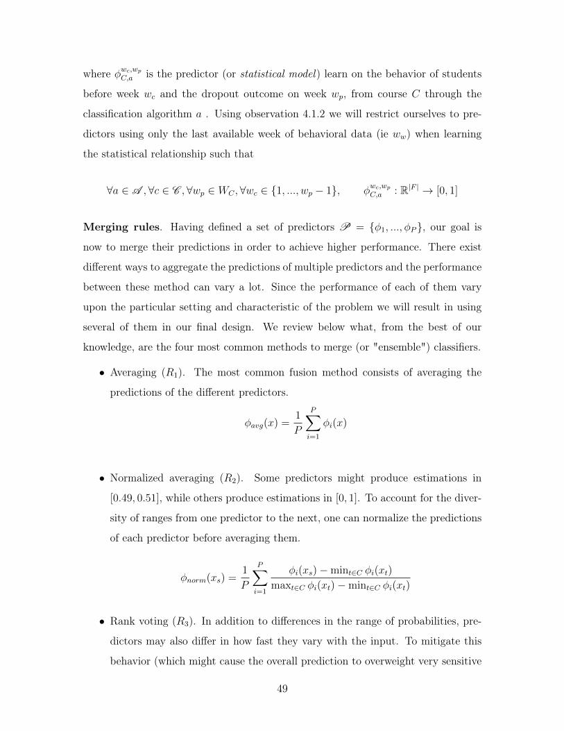
where 𝜑𝑤𝑐,𝑤𝑝

𝐶,𝑎 is the predictor (or statistical model) learn on the behavior of students

before week 𝑤𝑐 and the dropout outcome on week 𝑤𝑝, from course 𝐶 through the

classification algorithm 𝑎 . Using observation 4.1.2 we will restrict ourselves to pre-

dictors using only the last available week of behavioral data (ie 𝑤𝑤) when learning

the statistical relationship such that

∀𝑎 ∈ 𝒜 ,∀𝑐 ∈ 𝒞 ,∀𝑤𝑝 ∈ 𝑊𝐶 ,∀𝑤𝑐 ∈ {1, ..., 𝑤𝑝 − 1}, 𝜑𝑤𝑐,𝑤𝑝

𝐶,𝑎 : R|𝐹 | → [0, 1]

Merging rules. Having defined a set of predictors 𝒫 = {𝜑1, ..., 𝜑𝑃}, our goal is

now to merge their predictions in order to achieve higher performance. There exist

different ways to aggregate the predictions of multiple predictors and the performance

between these method can vary a lot. Since the performance of each of them vary

upon the particular setting and characteristic of the problem we will result in using

several of them in our final design. We review below what, from the best of our

knowledge, are the four most common methods to merge (or "ensemble") classifiers.

∙ Averaging (𝑅1). The most common fusion method consists of averaging the

predictions of the different predictors.

𝜑𝑎𝑣𝑔(𝑥) =1

𝑃

𝑃∑︁𝑖=1

𝜑𝑖(𝑥)

∙ Normalized averaging (𝑅2). Some predictors might produce estimations in

[0.49, 0.51], while others produce estimations in [0, 1]. To account for the diver-

sity of ranges from one predictor to the next, one can normalize the predictions

of each predictor before averaging them.

𝜑𝑛𝑜𝑟𝑚(𝑥𝑠) =1

𝑃

𝑃∑︁𝑖=1

𝜑𝑖(𝑥𝑠) − min𝑡∈𝐶 𝜑𝑖(𝑥𝑡)

max𝑡∈𝐶 𝜑𝑖(𝑥𝑡) − min𝑡∈𝐶 𝜑𝑖(𝑥𝑡)

∙ Rank voting (𝑅3). In addition to differences in the range of probabilities, pre-

dictors may also differ in how fast they vary with the input. To mitigate this

behavior (which might cause the overall prediction to overweight very sensitive

49

predictors), one can rank the probabilities within the target course first, then

average and normalize the resulting ranks of the different classifiers. That is, we

effectively replace the individual probabilities for each classifier by the ranking

of that probability among all the probabilities made by this classifier on the

same target course . For instance, if a classifier outputs {0.3, 0.5} as the prob-

abilities for two students, we will transform these into {1, 2} before combining

them with other classifier outputs.

𝜑𝑟𝑎𝑛𝑘(𝑥𝑠) =1

𝑃

𝑃∑︁𝑖=1

𝑟𝑎𝑛𝑘(𝜑𝑖(𝑥𝑠)) − 1

𝑁𝑡

where 𝑟𝑎𝑛𝑘(𝜑𝑖(𝑥𝑠)) refers to the rank of 𝜑𝑖(𝑥𝑠) in the set {𝜑𝑖(𝑥), 𝑥 ∈ 𝐶}.

∙ Stacking (𝑅4). Another successful technique to ensemble predictors is to learn

a so-called meta-model in order to use an optimal weighted average of when

merging predictions. This technique can be thought as a weighted version of 𝑅1

where the weights are learned through another classification predictors. Instead

of learning the statistical relationship between 𝑥𝑠 and 𝑦𝑠 a meta-model learns

the relationship between a set of predictions {𝜑1(𝑥𝑠), ..., 𝜑𝑃 (𝑥𝑠)} and the final

outcome 𝑦𝑠.

𝜑𝑠𝑡𝑎𝑐𝑘(𝑥𝑠) = Φ𝑎(𝜑1(𝑥𝑠), ..., 𝜑𝑃 (𝑥𝑠))

where Φ𝑎 : [0, 1]𝑃 → [0, 1] is a predictor learned through the classification

algorithm 𝑎.

Structure. We have seen that one can choose between several methods when merg-

ing predictions. We are now left with another choice when designing our final method:

which ensembling method to use ? Similarly to our choice to combine different predic-

tors, we choose to combine different ensembling methods. Instead of choosing a single

method we will apply several of same to the same set of basic predictors and then

combine their respective outputs. The idea to successively merge predictors naturally

leads to the notion of structure defined below.

Definition 5.1.1. Structure. We call structure 𝑠 on the set of predictors 𝒫, a

50

sequence of tuples (predictors,merging rules) that is successively used to create new

predictors and which results in a final predictor.

In figure 5-1 we illustrate how the order of the successive merges can influence

the final prediction (starting from the same basic predictions). This in no way states

that some structures are better than others, but at least gives an intuition on why

their performance can be different one from the other.

Figure 5-1: Illustration of two Ensembling structures yielding two different predic-tions. For this illustration we use a simple majority merging rule. Circles representbasic predictors while triangles stand for merge rules. The colors indicate a binarythe prediction.

We call layer of structure 𝑠 the set of predictors that are distant from the basic

predictors by the same number of merging process. That is, we call first layer of struc-

ture 𝑠 the set of predictors created by directly merging outputs from basic predictors.

Layer 2 of structure 𝑠 is formed by the predictors formed by merging predictors of

layer 1 on so on.

Figure 5-2 presents an example of a structure whose predictors {𝜑1, ..., 𝜑6} are

trained from three classification algorithms {𝑎1, 𝑎2, 𝑎3} on two source courses. Their

predictions are ensembled using a three layers structure and the four different merging

rules.

In the choice of our final ensembling structure to merge predictors, we will adopt a

machine learning point of view again, and explore try to explore the space of different

possible structures.

51

Figure 5-2: Example of an ensembling structure for dropout prediction based ontwo source courses and three different classification algorithms.

5.2 Experiments

We describe now three different frameworks we used to build predictive models. For

each one, we given the details on how we build models, test them and then report

results.

5.2.1 Single course - Multiple algorithms

Our first step away from the “Naive transfer” method is called the “Single course -

Multiple algorithms” framework. In this framework, predictive models are still built

from the data of one course only, but several algorithms are used (while the “Naive

transfer” method only used one).

Training Given a target course and a DPP ,

1. Choose one source course among the remaining courses

2. Train each of the four algorithms using 5-fold cross validation on this source

course .

52

3. Create a fused model, whose output is the average of the outputs of all four

models.

4. repeat from step 1 for all possible source course .

This procedure gives exactly twenty models (four algorithms plus a fused model,

repeated for all four possible source course ).

Evaluation Given a target course and a DPP , testing our twenty models on the

target course gives twenty AUC . For this target course we report aggregated results

over all DPP by using the DAUC metric introduced earlier (see section 4.1.2).

5.2.2 Concatenated course - Multiple algorithms

In the “Concatenated course” framework, we leverage all available data (from the

source courses) and follow a procedure similar to the “Single course-Multiple algo-

rithms” experiment.

Particularly, we artificially create a course by concatenating the data of all other

source courses. We call this artificially created course the concatenated course and we

note 𝐶 ′(𝒞 ) the concatenated course built from all the courses in 𝒞 . From now on we

include this additional course into the set of courses 𝒞 such that the set of predictors

can be defined similarly to equation 5.1.

Definition 5.2.1. Concatenated Course. We call a course Concatenated course

and note 𝐶 ′1−𝑛 a course artificially created by concatenating the data from a set of

source courses 𝒞 = {𝐶1, ..., 𝐶𝑛}. This assumes that we access the full data for all

courses in 𝒞 , ie {(𝑥𝑤𝑐𝑠 , 𝑦

𝑤𝑝𝑠 ),∀𝑠 ∈ 𝐶,𝐶 ∈ 𝒞 }.

Training Given a target course and DPP ,

1. Concatenate the data of all the possible source courses into a “concatenated

course”.

2. Train each of the four algorithms using 5-fold cross validation on this “concate-

nated course”.

53

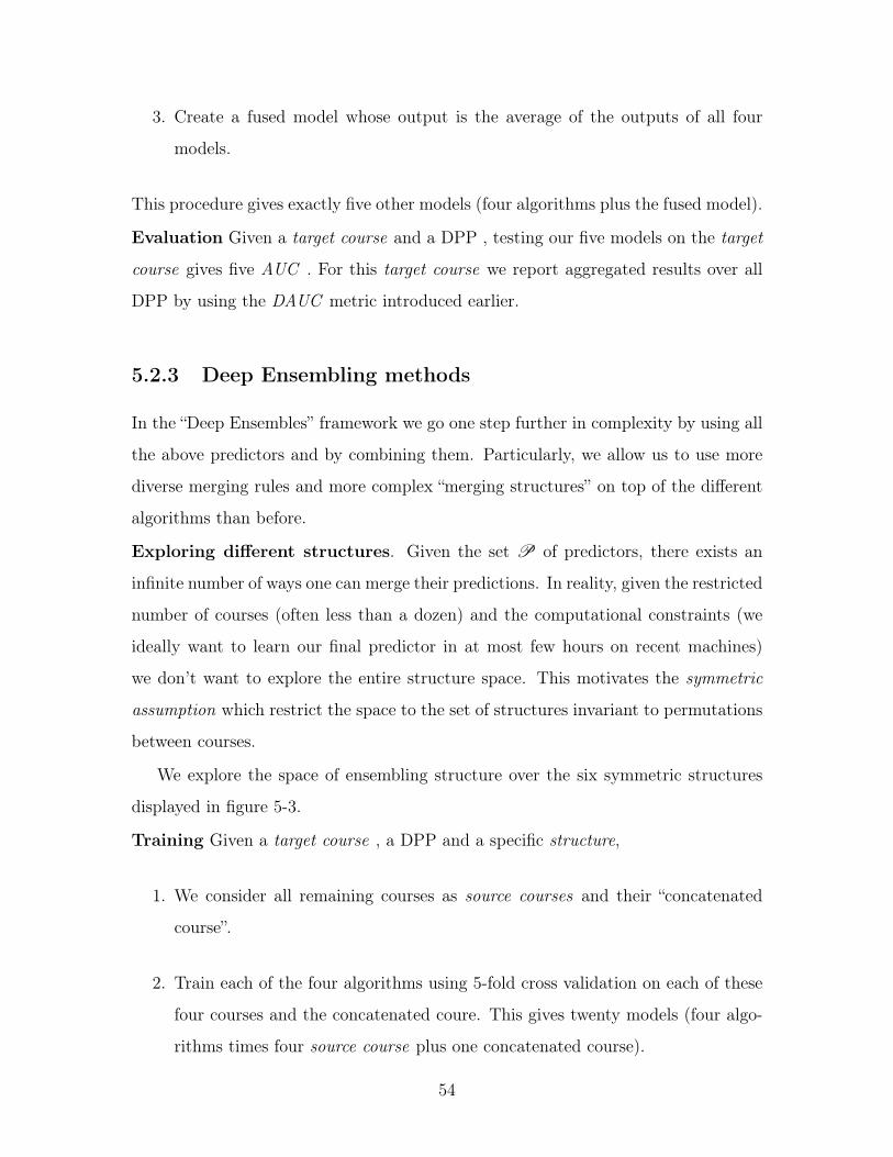
3. Create a fused model whose output is the average of the outputs of all four

models.

This procedure gives exactly five other models (four algorithms plus the fused model).

Evaluation Given a target course and a DPP , testing our five models on the target

course gives five AUC . For this target course we report aggregated results over all

DPP by using the DAUC metric introduced earlier.

5.2.3 Deep Ensembling methods

In the “Deep Ensembles” framework we go one step further in complexity by using all

the above predictors and by combining them. Particularly, we allow us to use more

diverse merging rules and more complex “merging structures” on top of the different

algorithms than before.

Exploring different structures. Given the set 𝒫 of predictors, there exists an

infinite number of ways one can merge their predictions. In reality, given the restricted

number of courses (often less than a dozen) and the computational constraints (we

ideally want to learn our final predictor in at most few hours on recent machines)

we don’t want to explore the entire structure space. This motivates the symmetric

assumption which restrict the space to the set of structures invariant to permutations

between courses.

We explore the space of ensembling structure over the six symmetric structures

displayed in figure 5-3.

Training Given a target course , a DPP and a specific structure,

1. We consider all remaining courses as source courses and their “concatenated

course”.

2. Train each of the four algorithms using 5-fold cross validation on each of these

four courses and the concatenated coure. This gives twenty models (four algo-

rithms times four source course plus one concatenated course).

54

C1

s1

C2 C3 C1 C2 C3

C1 C2 C3 C1 C2 C3

C1 C2 C3 C1 C2 C3

s2

s3

s5 s6

s4

Figure 5-3: Illustration of the six Ensembling Methods structures compared whenused with three source courses and three algorithms.

3. Train the structure (all the stacking rules of the structure) using the “concate-

nated course” as training set. That can be decomposed into steps

(a) Apply the twenty models to the “concatenated course’ data.

(b) Using the outputs of these models as new “features”, train the logistic

regression models used in the 𝑅4 rules of the first layer of the structure.

(c) repeat the step above for all layers of the structure.

This procedure gives a single model corresponding to the structure picked at the

beginning.

55

Evaluation Given a target course and a DPP , we test the corresponding model for

all the six structures described earlier on the target course . We then evaluate the

DAUC over all the DPP by taking into account the six models. To see statistically

significant differences between the different structures we had to aggregate one step

further. We average the DAUC over all five target courses.

5.3 Results

We present the results obtained by following the evaluation framework for the three

frameworks on our datasets. After explaining the results and highlighting key findings,

we show that we are able to use a model built on the firt five edX courses to successfully

predict dropout on ten Coursera courses.

5.3.1 Single course - Multiple algorithms

To evaluate the Single Course - Multiple Algorithms framework we use 𝐶0 as the

target course and {𝐶1, 𝐶2, 𝐶3, 𝐶4} as the four possible source courses (see 3.1). We

also use the four algorithms described in

Figure 5-4 reports the DAUC (in bold) as well as the standard deviation of the

performance (in parenthesis). For instance, we read from this figure that a logistic

regression (algorithm 𝑎1) trained on 𝐶1 has an average DAUC of 7.8 with a standard

deviation of 9.6.

As noticed before, we remark that models built from different courses perform

significant differently. Moreover, we remark that this very little depends on the choice

of the algorithm. For a given target course , some courses are therefore better suited

to build good predictive models than others.

Fused models perform better For half of the source courses, the fused model

(model obtained from a 𝑅1 merging rule to merge outputs of the four algorithms)

performs better than the best individual model. When this is not true, the fused

model still performs almost identically to the best individual model (3.9 instead of

3.7 for 𝐶1 and 4.6 instead of 4.5 for 𝐶3). On average over the four courses, the choice

56

a1 a2 a3 a4 s1

C1

C2

C3

C4

7.8 7.0 5.8 3.7 3.9

18.3 9.0 6.3 5.7 5.0

15.8 7.3 4.5 5.7 4.6

6.6 6.4 4.1 4.3 3.5

(9.6) (7.3) (5.8) (2.0) (4.0)

(10.8) (7.4) (4.8) (2.4) (2.9)

(11.7) (5.8) (2.5) (2.7) (2.7)

(5.4) (5.0) (2.3) (2.3) (2.1)2

4

6

8

10

12

14

16

Figure 5-4: Performance on target course 𝐶0 of the different “Single course” meth-ods to build predictive models. Displayed is the average (standard deviation) of theDAUC over all possible DPP (less is better).

of the fused model is the best choice.

5.3.2 Concatenated course - Multiple algorithms

We now use a framework very similar to previous one. We simply use the concatenated

courses of {𝐶1, 𝐶2, 𝐶3, 𝐶4} as our only source course and evaluate the results according

to the same framework than before on course 𝐶0.

In figure 5-5 we reuse (for clarity) the results of the Single Course - Multiple

Algorithms framework and added the results of the Concatenated Course - Multiple

Algorithms framework in the last row.

Concatenating courses yields better performance than single courses We

remark that for every algorithms, using the concatenated course as training set yields

better performance on the target course than using the “best” individual source course

. Moreover, the difference is significant for all algorithms (the is decreased by between

25% and 50%).

Fused models on concatenated course, best model so far The best results

57

a1 a2 a3 a4 s1

C1

C2

C3

C4

C ′1−4

7.8 7.0 5.8 3.7 3.9

18.3 9.0 6.3 5.7 5.0

15.8 7.3 4.5 5.7 4.6

6.6 6.4 4.1 4.3 3.5

3.2 4.8 3.1 3.1 1.6

(9.6) (7.3) (5.8) (2.0) (4.0)

(10.8) (7.4) (4.8) (2.4) (2.9)

(11.7) (5.8) (2.5) (2.7) (2.7)

(5.4) (5.0) (2.3) (2.3) (2.1)

(3.7) (2.9) (1.6) (2.2) (1.6)2

4

6

8

10

12

14

16

18

Figure 5-5: Performance on target course 𝐶0 of the different “Single course” meth-ods as well as the “Concatenaed” method. Displayed is the average (standard devia-tion) of the DAUC over all possible DPP (less is better).

are achieved when using the concatenated course as training set and leveraging the

simple ensembling method described above (fused model). This method is both the

best on average (50% better than the second best method) and has the lowest standard

deviation.

Moreover we remark that such method offers the advantage to remove the hurdle

of “choice”. Before applying a predictive model in a real-life setting, one needs to

choose which model to use. Choosing the concatenated course with a fused model

allow the user to avoid choosing both the course and the algorithm used to train the

model.

5.3.3 Deep ensembling methods

We now evaluate the more complex structures described in 5-3. We independently

aggregate the DAUC obtained over two sets of DPP ’s.

∙ DPP refers to all common DPP as before.

∙ 𝐷𝑃𝑃𝑠ℎ𝑜𝑟𝑡 refers to all common one-week-ahead DPP .

58

This enables us to discover particularly interesting findings.

Figure 5-6 shows the average DAUC over the two sets of DPP ’s. In addition to

the performance of the six structures, we reported the results for the fused model on

concatenated courses (the best model from the previous experiments) as “Concat”.

At the top we can see that all structures have similar performance. We remark

however, that the more complex structure 𝑆6 seems to yield better performance on

average.

𝑆2 structure is the best for one-week-ahead DPP Major performance differ-

ences between these structures come when we consider only one-week-ahead prediction

problems. For these problems we observe that 𝑆6 still performs better that most of

the other structures. However 𝑆2 yields by far the best results. The result of the

bottom graph of figure 5-6 should read as follows : over one-week-ahead DPP , the

AUC of 𝑆2 is on average only 0.01 worst than the best available model for that DPP .

5.3.4 Transferring across MOOC platforms

To complete our demonstration we now put ourselves in a real-world setting where

given data from past courses in a certain platform, we aim at performing predictions

on new set of courses, from a different platform. We take our five first courses from

edX platform as our source courses and consider successively the ten courses from

Coursera to be our target course. We assume to have access to the full data of the

first five courses but only the behavioral data for the last ten (no dropout status).

Finally, we test our prediction against the ground truth for the last ten courses (using

the true outcomes).

The results in figure 5-7 show the average performance of three methods when

tested on the ten Coursera courses. We see again that a 𝑆2 structure seems to perform

best (which confirm previous results obtained when testing on courses from the same

platform).

Now that we convinced ourselves that the 𝑆2 structure performs best even on

courses from another platform, it is time to come back a metric easier to interpret.

Figure 5-8 describes the AUC scores of the 𝑆2 structure trained on the five edX

59

𝐶𝑜𝑛𝑐𝑎𝑡 𝑆1 𝑆2 𝑆3 𝑆4 𝑆5 𝑆6

0

2

4

6·10−2

Ave

rage

DAU

Cov

er𝐷𝑃𝑃

𝐷𝑃𝑃

𝐶𝑜𝑛𝑐𝑎𝑡 𝑆1 𝑆2 𝑆3 𝑆4 𝑆5 𝑆6

0

2

4

6·10−2

Ave

rage

DAU

Cov

er𝐷𝑃𝑃𝑠ℎ

𝑜𝑟𝑡

𝐷𝑃𝑃𝑠ℎ𝑜𝑟𝑡

Figure 5-6: Average (standard deviation) DAUC of different structures. 𝐷𝑃𝑃refers to all Dropout Prediction Problems common to the five courses while𝐷𝑃𝑃𝑠ℎ𝑜𝑟𝑡 refers to one-week-ahead Dropout Prediction Problems only.

60

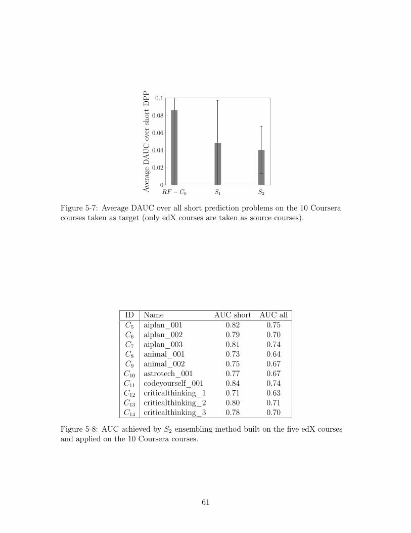
𝑅𝐹 − 𝐶0 𝑆1 𝑆2

0

0.02

0.04

0.06

0.08

0.1

Aver

age

DA

UC

over

shor

tD

PP

Figure 5-7: Average DAUC over all short prediction problems on the 10 Courseracourses taken as target (only edX courses are taken as source courses).

ID Name AUC short AUC all𝐶5 aiplan_001 0.82 0.75𝐶6 aiplan_002 0.79 0.70𝐶7 aiplan_003 0.81 0.74𝐶8 animal_001 0.73 0.64𝐶9 animal_002 0.75 0.67𝐶10 astrotech_001 0.77 0.67𝐶11 codeyourself_001 0.84 0.74𝐶12 criticalthinking_1 0.71 0.63𝐶13 criticalthinking_2 0.80 0.71𝐶14 criticalthinking_3 0.78 0.70

Figure 5-8: AUC achieved by 𝑆2 ensembling method built on the five edX coursesand applied on the 10 Coursera courses.

61

courses. We report the average AUC over all DPP and over all short DPP . We

remark that we have achieved satisfying performance on both sets of DPP . More

particularly, we remark that the algorithm achieves AUC of around .8 for short DPP

and of around .7 on average over all DPP .

These results should be put in perspective by looking at the results achieved by

a Naive transfer method and presented in figure 4-5. The AUC of one-week-ahead

DPP were located around .6 on average. Reaching .8 AUC on average over one-week-

ahead DPP , while transferring to courses from another platform, is therefore a non

significant improvement.

5.3.5 Releasing a Package for Ensembling Methods

In the previous section, we explained how ensembling methods can successfully help

building predictive models in the context of MOOCs. We showed that in some cases

(one-week-ahead prediction problems), ensembling predictors built from diverse data

sources performed significantly better than any individual model (even models trained

on from the concatenation of courses’ data).

In this section we introduce a python library enabling such predictive models to

be built. After laying out the motivation for such tool, we describe its main features

and give concrete use cases for it.

Motivation. Most of existing libraries to automate the creation and use of ensem-

bling methods rely on the same few principles. They all produce multiple predictors

by "subsampling" a single dataset at random. "Subsampling" here refers to one of

the two or both following procedures

∙ Subsampling a subset of samples out of the initial dataset

∙ Subsampling a subset of the features out of the set of features and then consid-

ering all samples.

Various techniques can be designed by changing the way both subsampling are done.

For example, a famous paradigm is to subsample the samples with replacement. Such

62

technique is called Bagging 3.

As shown in the previous section, selecting at random samples out of the initial

dataset is not always the best strategy. When one can access additional information

about the origin of each sample (namely, we know that certain samples come from

certain datasets) taking advantage of this knowledge appears to be useful. This

is particularly relevant in the context of Dropout Prediction on MOOCs, because

different origins are often needed to build a well-performing model.

To the best of our knowledge, no existing tools offer to facilitate the effort of build-

ing and merging predictors out of multiple data sources. With Deep ensembling, a

python open-source library to train and merge predictors from multiple data sources,

we offer the first tool to facilitate this journey. Deep ensembling4 is an open-source

code package written in python that enable users to train and ensemble classifiers on

multiple datasets. The capabilities of this framework can be described as three main

components.

Training classifiers on multiple datasets. Given a set of 𝑛 data sources for

which we observe both the features {𝑋1, .., 𝑋𝑛} and the outcomes {𝑦1, ..., 𝑦𝑛}, we

want to train multiple classifiers. Instead of simply using a Bagging method on the

concatenated data (which will artificially create multiple datasets by subsampling

the samples at random) we want to build independent classifiers on each of the data

sources.

Deep ensembling allows users to specify the type of classification algorithms to

learn and the range of the parameters to try as shown in the figure 5-9. Each of the

classification algorithm is trained using the corresponding sklearn method and the

parameters are optimized through 5-fold cross-validation. The trained predictors are

returned in a python dictionary.

Defining and training ensembling structures. Having trained the predictors,

we now explain how users can define ensembling structures to combine them. After

3http://scikit-learn.org/stable/modules/ensemble.htmlh19984https://github.com/sebboyer/Deep_ensembling

63

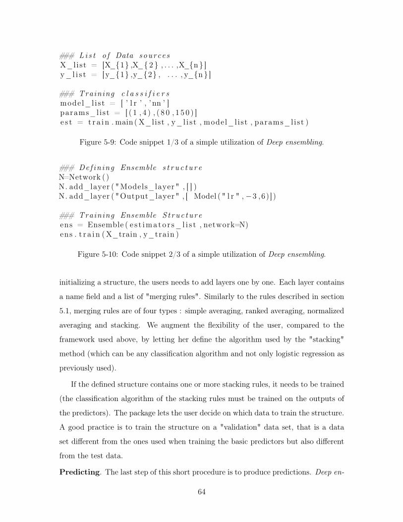
### Li s t o f Data sourcesX_list = [X_{1} ,X_{ 2 } , . . . ,X_{n } ]y_ l i s t = [y_{1} ,y_{2} , . . . , y_{n } ]

### Training c l a s s i f i e r smodel_l i s t = [ ’ l r ’ , ’ nn ’ ]params_list = [ ( 1 , 4 ) , ( 8 0 , 1 5 0 ) ]e s t = t r a i n . main ( X_list , y_l i s t , model_l ist , params_list )

Figure 5-9: Code snippet 1/3 of a simple utilization of Deep ensembling.

### Def in ing Ensemble s t r u c t u r eN=Network ( )N. add_layer ( "Models_layer " , [ ] )N. add_layer ( "Output_layer" , [ Model ( " l r " , −3 ,6) ] )

### Training Ensemble S t ruc tu reens = Ensemble ( e s t ima to r s_ l i s t , network=N)ens . t r a i n ( X_train , y_train )


initializing a structure, the users needs to add layers one by one. Each layer contains

a name field and a list of "merging rules". Similarly to the rules described in section

5.1, merging rules are of four types : simple averaging, ranked averaging, normalized

averaging and stacking. We augment the flexibility of the user, compared to the

framework used above, by letting her define the algorithm used by the "stacking"

method (which can be any classification algorithm and not only logistic regression as

previously used).

If the defined structure contains one or more stacking rules, it needs to be trained

(the classification algorithm of the stacking rules must be trained on the outputs of

the predictors). The package lets the user decide on which data to train the structure.

A good practice is to train the structure on a "validation" data set, that is a data

set different from the ones used when training the basic predictors but also different

from the test data.

Predicting. The last step of this short procedure is to produce predictions. Deep en-

64

### Test ing Ensemble s t r u c t u r ey_pred = ens . network . p r ed i c t ( X_test )


sembling allows user to use a syntax similar to that of sklearn to produce predictions

from a trained structure as shown in figure 5-11. Under the hood, the function first

applies each of the basic predictors to the test set, then it combines these predictions

using the predefined rules of the first layer, then combine those combinations using

the predefined rules of the second layer and so on until reaching the final combination

which provides a simple probability for each sample.

Use-case of Dropout Prediction If the package provides a rather general frame-

work to trained complex ensembling structures from different datasets, this tool is

particularly relevant to build predictive models in the context of MOOCs. When

several courses worth of data are available, we saw in this section that ensembling

structure provided a good way to build predictive model that "transfer" well to other

classes. To build such models we used exactly the framework enabled by this package.

We hope that such tool will help the MOOC research community adopt a point

of view more focus toward models’ ability to "transfer" well to other courses.

65

Chapter 6

Deploying a Dropout Prediction

System

In the previous chapters, we explained the motivation for a dropout prediction system,

the main challenges that it brings as well as theoretical solutions that we developed

to tackle them. We are now left with a set of features and statistical models that

together can predict dropout of students on new MOOC courses with a reasonable

precision. The idea behind the remaining challenges can be summarized by one word

: deployment. Particularly, how can we build systems to facilitate the wide adoption

of such solutions in order to maximize its impact on MOOCs across the world?

6.1 Motivation and Deployment Opportunities

In this first section, we explore two specific means of adoption that we tested. The

first relies on an industry partner (edX) and the second is focus on a public release of

our solution. We discuss advantages and limits of both and explain why we pursued

the second option further.

6.1.1 Partnership with a leading MOOC provider

We discuss our partnership with EdX which was crucial to bring this project to life

and then explain why we finally choose to use a more general way to deploy our

67

solution.

Successful Data Sharing Partnership. EdX was our first partner and our main

data provider (they provided the first five courses used in this work). As a main

stakeholder of this project, they have been involved with us throughout the year. We

had met multiple times with their product team to present our advances and to make

sure our work was aligned with the needs of their teachers and their data analysts.

Such project would have been immensely more difficult (if not impossible) without

the head-start given by their willingness to share some of their student data with us

(under strict scrutiny of the relevant regulation).

Meetings with the product team have been helpful to prioritize ideas throughout

the year. One example is the design choices that the team helped us to make as

we were deciding on the best outputs to provide to teachers. At first, we thought

that the individual probability for each student to dropout was the most relevant

metric. Instead, they suggested to group students in clusters of dropout “risk” and to

categorize students in different clusters. This will arguably make the output easier

to understand for teachers and more importantly easier to act upon (teachers could,

in the future, directly send additional resources and motivation emails to a certain

cluster of students).

Choice of a broader deployment. Since our goal is to provide a solution for MOOC

any platforms to perform dropout predictions, we choose to open our solutions to a

broader community by releasing publicly the solutions we developed.

This deployment strategy has proved to be successful as we managed to get another

research group (from the University of Edinburgh) to use our solutions.

6.1.2 Purposes of Large Scale Public Deployment

We set in this section the goals of our deployment both in term of audience and in

terms of impact.

Targeted audience. Our targeted audience can mainly be summarized in three

categories, each of which may have different use cases for a Dropout Prediction system

:

68

∙ MOOC providers, whose incentives are often link to the completion and the

certification rate of their cohort students.

∙ MOOC teachers, who could use these insights to adapt and customize their

course to their cohort of students.

∙ The scientific community who work with these data to better understand learn-

ing pattern and behavior.

It is important to note here that we are not restricting ourselves anymore to a

particular MOOC platform but hope to reach these categories in multiple ones. As

mentioned in the introduction of this thesis, about half of the MOOC courses are

hosted by platforms outside the top two platforms. This makes the ability to reach

to more than one platform particularly important.

The diversity of this targeted audience doesn’t come without difficulties for the

ones willing to share a single system with them. In addition to the different use cases

that each of them may have, they may also have different technical background which

make the design of a single solution challenging as we will see next.

Targeted Impact. What do we want to achieve by sharing such a system ? Given

the diversity of the potential beneficiaries of such system, what are the minimum

capabilities such system should have to benefit to all ? In order to design an efficient

system, we start by stating clearly the impact that we expect our system to have in the

mid-term. After reviewing the particular needs of each of the following stakeholders :

MOOC providers, MOOC teachers, Scientists; we have narrowed the intended benefit

to the following three points:

∙ Changing the behavior of teachers on MOOCs toward more adaptation and

customization. We hope that given real-time information about which and how

many of their students are “at risk” of dropping out, teachers will be encouraged

to adapt their content and even customize it to the needs of their students while

the course is given. This could means to adapt the level of the quizzes to the

current “dropout risk” of the class for example.

69

∙ Increasing the retention rate of students. Either through the actions following

the remark above, or through direct intervention from MOOCs providers we

hope that such information will help convince certain students to stay longer

in courses. A MOOC platfrom could for example use the “dropout risk” of

students to reach out to those slightly at risk and try to incentives and help

them through more resources or motivation emails.

∙ Making analytics-based research on MOOCs easier for scientists. We hope this

system to benefit the scientific community as a whole. By accessing easy-to-

generate dropout predictions, scientists could rapidly use them in their research.

For example, a research group working on the impact of collaboration among

students on their performance could study the correlation between these collab-

orations and the dropout risk of students.

6.2 Challenges of Deploying a Machine Learning Pipeline

Having described the targeted audience and impact, we now present what constraints

should be taken into account when building our system. In this section, we first

describe in details the different steps of our solution : “Translation”, “Extraction”,

“Prediction”. We then explain what are the specific challenges associated with De-

ploying a Dropout Prediction System compared to other machine learning services.

Figure 6-4 illustrates these three steps and their relationship one with another. The

dotted arrows indicate that a user could choose to use not only the entire system but

also one or two specific steps of this system.

6.2.1 Translation Step

The first step of the process is to transform the raw log files into a structured MySQL

database. We called this step the “Translation step”.

Purpose and Description. The input of this first step are typically log files (in

.JSON format) capturing different physical events happening on the platforms such

70

Translation Extraction Prediction

LOG FILES DATABASE FEATURES

Figure 6-1: Three independent steps of the Dropout Prediction Process

Tables in MySQL databaseagentanswer

assessmentsobserved_events

osproblem_types

problemsresource_types

resourcesresources_urlssubmissions

urls

Figure 6-2: List of tables populated in the MySQL database by the "Translationstep".

as : Video played, Video paused, Problem showed, Submission, Book access, Forum

access. These events are recorded along with some meta-data related to the student,

the time and the interface used for each of them. This data is all the information

available to us about the behavior of students in a course but they are hard to use

for statistical learning purposes in its current shape.

A ’Translation step’ is therefore necessary to transform this data into a format

easier to query. To do so our solution parse the events one after the other and populate

a structured database (MySQL format is used). Figure 6-2 gives the names of the

different tables populated from the events in the log files. One can now query this

table using classic MySQL syntax.

71

Accessibility - Flexibility tradeoff. We remind the reader that in the context of

Dropout prediction envisioned here, we want to provide a solution to enable not only

data analysts but also teachers and course staff to make predictions.

Since the "Translation step" is the most likely to be dependent on the data for-

mat, it is also the most likely to require high degree of customization. To enable

these changes to be made efficiently, we will choose to provide a very flexible solution

(using open source software) even though this makes it less accessible to non-technical

persons (such as MOOC teachers in general).

6.2.2 Extraction Step

Now that we have transformed our data into an easy-to-query format, we can start to

extract the relevant features from this database. We call this the "Extraction Step".

Purpose and Description. The goal of this step is to automate the extraction,

from the structured database, of a set of user-defined features.

The input of the “Extraction step” is therefore twofold.

∙ First it needs a MySQL database, similar to the output of the “Translation

step”, containing the relevant information about the different type of events

that happened during the class.

∙ Second it needs a set of "feature-defining" scripts. These need to be written in

the format of “.sql” scripts that can query the structured database and combine

the information contained to create higher level feature. These scripts can be

written by any third party as long as it uses the format of the above-mentioned

SQL database.

Given these two types of inputs, our “Extraction step” automates the extraction

of the set of features on the MySQL database. This typically generates for each

student, each feature type and each week of the MOOC course, a particular value.

For instance, figure 6-3 illustrates the extraction of the feature "Number of lectures

watched in a week" on a MOOC course database.

72

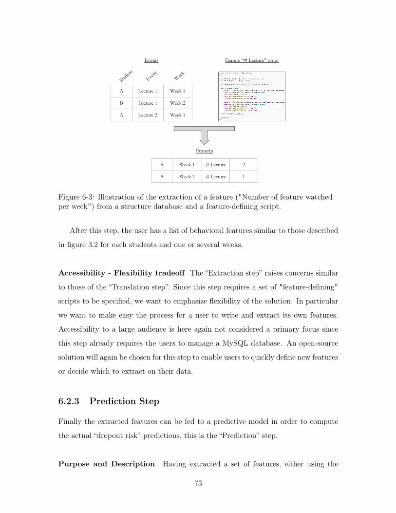
Events

A Lecture 1 Week 1

B Lecture 1 Week 2

A Lecture 2 Week 1

Studen

t

Event

Week

Feature “# Lecture” script

A Week 1 # Lecture 2

B Week 2 # Lecture 1

Features

Figure 6-3: Illustration of the extraction of a feature ("Number of feature watchedper week") from a structure database and a feature-defining script.

After this step, the user has a list of behavioral features similar to those described

in figure 3.2 for each students and one or several weeks.

Accessibility - Flexibility tradeoff. The “Extraction step” raises concerns similar

to those of the “Translation step”. Since this step requires a set of "feature-defining"

scripts to be specified, we want to emphasize flexibility of the solution. In particular

we want to make easy the process for a user to write and extract its own features.

Accessibility to a large audience is here again not considered a primary focus since

this step already requires the users to manage a MySQL database. An open-source

solution will again be chosen for this step to enable users to quickly define new features

or decide which to extract on their data.

6.2.3 Prediction Step

Finally the extracted features can be fed to a predictive model in order to compute

the actual “dropout risk” predictions, this is the “Prediction” step.

Purpose and Description. Having extracted a set of features, either using the

73

“Extraction step” or another tool, one need to choose what to predict. We introduced

in the previous chapter the notion of a prediction problem. Depending on the current

timing of the course and the targeted prediction, the predictive model will be different.

The two dimensions needed to choose a model for Dropout Prediction are therefore

∙ The set of features extracted. A predictive model using 20 features as inputs

can’t be used on a 10 features dataset. Users therefore need to choose a predic-

tive model that matches their extracted features.

∙ The targeted prediction. This refers to the week number for which the dropout

prediction needs to be made. Given a set of features extracted on week 𝑤𝑐, the

predictive model used to predict dropout on week 𝑤𝑐 + 1 is different than the

predictive model used to predict on week 𝑤𝑐 + 2, ... .

The output of the “Prediction step” is a Dropout Prediction probability (a real

number between 0 and 1) for each student in the course.

Accessibility - Flexibility tradeoff. The "Prediction step" is likely to be less

subject to changes. Given a set of behavioral features, the user needs to be able to

produce dropout predictions for some week in the future. Apart from the choice of the

week to predict on and the set of behavioral features to be used, the logic of this last

step will remain relatively similar across the different users. Moreover, since this step

gives the final insights on the students, we are more concerned about this solution

being accessible to a broad user base (from Data analysts to MOOC teachers). We

will therefore choose a web interface to provide a solution to this last step.

6.2.4 Specific Challenges to Dropout Predictions

Having described the three steps required to go from log files to predictions we now

justify the need to build separate solutions for each of them. We argue that the di-

versity of format on MOOCs makes difficult other alternatives. Finally we compare

the challenges faced in the context of MOOCs with the challenges faced by another

74

research community used to releasing machine learning services.

Diversity of formats. One of the major challenge when using data from MOOCs

comes from the diversity of formats. This diversity, in turns, comes from two factors

:

∙ the large number of MOOC platforms and their courses. For instance, the

two main MOOC platforms (edX and Coursera) don’t share the same syntax

when recording certain “events” (such as a user playing a video). In addition

to not using the same syntax to record logs, different courses (even from the

same platform) generally contain different types of events. For instance, some

courses (such as 6002x from edX given in th fall 2012) contain a “wiki” resource

(a set of web-pages summarizing important knowledge from the course) while

others (such as 1473x given in the spring 2013) don’t.

∙ the rapid evolution of MOOC user interfaces and capabilities. This evolution

entails that new types of events are constantly created and added in log files.

For instance, a new “Warm-up” section, containing highlevel description of the

content to come, is now available on edX courses. This means that a new type

of resource is present in the log files.

The natural diversity of formats imposes that our system be flexible. The Trans-

lation, Extraction and Prediction steps presented in the previous section shouldn’t

therefore be concatenated into a single rigid software. Such a software, taking raw log

files as inputs and releasing dropout predictions as outputs, would put too much con-

straints on the format of the input data. This will considerably restrict the spectrum

of potential users. Instead, we built independent solutions for these three steps. Each

of these steps can therefore be used independently from the others and they commu-

nicate only through the data that is transferred from one to the other as shown in

figure 6-4.

If a particular user possesses raw log files in one of the format supported by the

“Translation step” for example, this user can use the entire pipeline by successively

75

feeding the output of one step to the next. She will therefore be able to go from raw

log files up to dropout predictions.

More interestingly, if a similar user has slightly different log file format (the events

are recorded using a slightly different syntax), our system can still be useful. Instead

of using our solution for the Translation step, this user will choose to translate her

data using a different solution (probably by adapting the code of our solution to her

own needs). Once the data is translated into the desired structured format, she could

leverage the rest of the solutions by feeding the results of her customised “Translation

step” to the “Extraction” and the “Prediction” steps, thus going from a structured

database to dropout predictions.

Finally, if a user has gathered behavioral features through another process (differ-

ent from our “Extraction” step solutions but respecting the same feature definitions),

she will still be able to leverage our solution for the "Prediction" step and therefore

transform her set of behavioral features into dropout predictions.

Having build independent solutions for each of the three steps of our process en-

ables use to provide a solution that handle the diversity of formats on MOOCs.

Comparison with the Computer Vision community. The Computer Vision

community has been particularly use to sharing publicly machine learning models in

order to prove their performance. Typically, a research group will define new visual

features or new neural network architectures that work particularly well on a certain

well-defined problem. They will gather a relevant dataset and train a novel model

on this. An increasing proportion of scientist in this community will not only release

the methods (e.g., a scientific paper containing the neural networks structures, ...)

but also the actual pretrained models (a model that could be used as it is to produce

predictions on new images).

The most common ways for this community to share its machine learning models

has been by writing these pretrained models in a format understood by commonly

used code libraries. For instance, the Model Zoo 1 in the Caffe library (a DeepLearning

1https://github.com/BVLC/caffe/wiki/Model-Zoo

76

library developed by the university of Toronto) has gathered dozens of pre-trained

models developed by scientists across the globe. These models are accessible through

the use of the software library but also through other libraries (by using open source

translation softwares).

The key difference between the problems faced by the Computer Vision community

and those in the Dropout Prediction community lie in the complexity and diversity of

the input formats that they need to handle. Where the Computer Vision community

needs to handle from two to ten fixed image or video format, our problems intrinsically

requires to deal with various and constantly changing data formats as showed above.

This explains why the solutions developed in this project are significantly different

from the ones developed by the Computer Vision community.

6.3 Multi-steps Deployment

In the last section of this chapter we describe the technical solutions adopted for each

of the three steps of our Dropout Prediction system. After justifying our choice of

solutions for each of them, we focus our attention into the capabilities of the web

platform built to deploy the “Prediction step”, because this step is arguably the most

impactful.

6.3.1 Technical Solutions for the Three Steps

In this section we remember the flexibility and accessibility constraints mentioned

earlier and conclude on the most appropriate technical solutions to release the three

steps. We start by explaining why Data Privacy concerns have made it impossible to

choose an API service as a means of deployment for any of the three steps. We then

justify the choice of two different deployment solutions.

The Question of Data Privacy . The three steps have one challenge in common

: respecting Data Privacy. Because student’s behavioral data is considered sensitive

and is protected by the law, any deployment solution must make sure it respect its

77

privacy. For instance, an API (Application Program Interface) won’t be a suitable

solution (for any of the steps) since it requires the service provider (the owner of the

API) to get proper authorization on the data that needs to be treated.

Any technical solution that we choose to deploy a step must therefore be easy to

use in compliance with data privacy regulation. That is, we want our solutions to

restrict the access to data to the user of the solution (and not to the provider of the

solution). We will use two technical solutions that comply well with this requirement

: Open source software, Web-platform with in-browser computation.

Open sourcing Translation and Extraction. We choose to release the first two

steps of the system using open-source code. The code is released as a set of scripts

publicly available on Github 2 and each of the first two steps is available as an inde-

pendent repository.

This method is appealing because it removes the maintenance effort from the

provider’s side (no need to maintain hardware) and remove at the same time any

Data Privacy concern from the user end (user download the software and then use

it on their own machine thus removing the concerns of a third party accessing their

data). The flexibility requirement (possibility for users to adapt the software to

their particular data format) is fulfilled because the code can easily be changed once

downloaded.

Open-source software also offer the possibility for users to contribute to it. For

example, a user adapting part of the software to handle her own data format could

easily make the changes available to others. The same thing is true for "feature-

defining" scripts. Even-though a good number of them are already available on the

repository, users can contribute by writing their own "feature-defining" scripts.

Web application for Prediction. The open source solution didn’t entirely meet the

"accessibility" requirement that we had fixed. Therefore, we looked for other technical

solution that will enable a broader range of people (not only technical persons who

2https://github.com/MOOCdb/Translation_software

78

are able to download a software on Github, but also less technical persons).

The most suitable solution for deploying the Prediction step of our system appears

to be a web platform. A web platform allows non-experts to use and interact very

easily with the models through an user-friendly interface. The data privacy concern

is taken care of by using client-side (Javascript) computation when dealing with data.

Thus, a browser-based solution solve the data privacy issue in addition to fulfilling the

accessibility requirements. Moreover, a browser-based platform is a very light-weight

solution from a maintenance point of view. Since all the calculation happens locally at

the user’s end, the burden of maintaining high performing hardware is removed from

the provider’s side. In the next section we dive into more details on the characteristics

of this web platform and describe the challenges faced and overcome while developing

it.

6.3.2 MyDropoutPrediction : a Web Platform for Dropout

Prediction

We explore in this sections the main challenges encountered when designing and

building an online platform for Dropout Prediction. We first explore the technical

challenges associated with the difficulty to perform advanced analytics directly in a

browser (in order to respect data privacy constraints).

In Browser Machine Learning. The first challenge faced when starting to design

such a platform was the difficulty to “transfer” to Javascript the complex models de-

scribed in section 4. This difficulty mainly emerge from two factors : the relative lack

of machine learning models in client-side languages such as Javascript, the assump-

tion that the computing power of the client machine is limited (therefore constraining

the complexity of models that can be supported).

We are therefore left with a tradeoff between the speed at which we want the com-

putation to occur and the expected accuracy we need to reach. In order to ensure that

models will run in a near-real time fashion for the practical size of the data at stake,

79

Data Insights Model

Server sideClient side

Figure 6-4: Sharing machine learning models through a web-browser separate theneed to share data with the service provider.

we decided to use a simplify version of the algorithms described in 4. In particular,

we restrict the set 𝒜 of algorithms to logistic regression alone. This classification

algorithm is significantly less computationally costly than the others while achieving

relatively good performances on all use cases explored so far (cf figure 5-4). We im-

plemented a 𝑆2 structure, therefore training the logistic regression separately on the

different courses and learning a meta-model on top of their predictions to produce

the final estimator.

Another advantages of the logistic regression classification algorithms compared

to other algorithms is that it is the simplicity of the associated decision algorithm.

In contrary to other classification algorithms such as random Forest, a trained logis-

tic regression is therefore easy to transfer from one language to the other, making

it possible to train and test in two separate language. Practically, we trained our

models using Python and transfer the learned weights through Javascript variables.

We then used these variables to build the final decision function corresponding to the

80

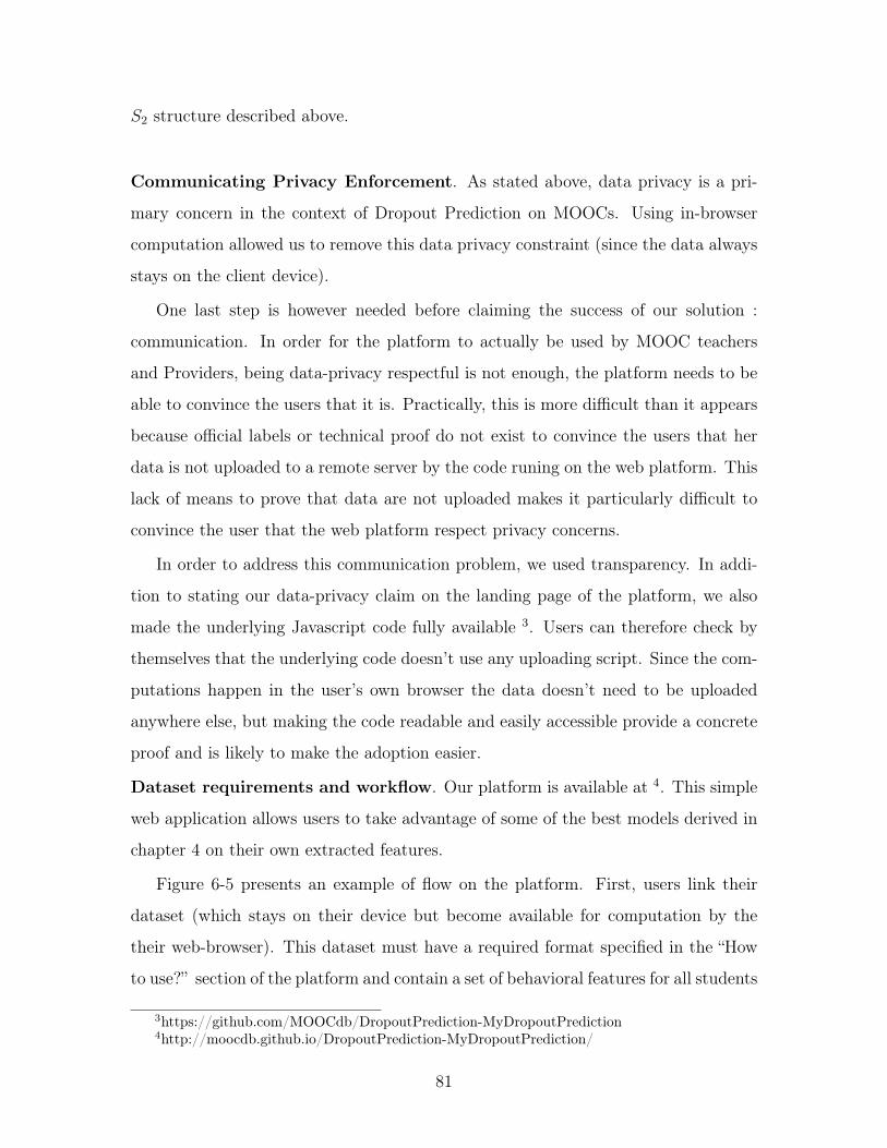
𝑆2 structure described above.

Communicating Privacy Enforcement. As stated above, data privacy is a pri-

mary concern in the context of Dropout Prediction on MOOCs. Using in-browser

computation allowed us to remove this data privacy constraint (since the data always

stays on the client device).

One last step is however needed before claiming the success of our solution :

communication. In order for the platform to actually be used by MOOC teachers

and Providers, being data-privacy respectful is not enough, the platform needs to be

able to convince the users that it is. Practically, this is more difficult than it appears

because official labels or technical proof do not exist to convince the users that her

data is not uploaded to a remote server by the code runing on the web platform. This

lack of means to prove that data are not uploaded makes it particularly difficult to

convince the user that the web platform respect privacy concerns.

In order to address this communication problem, we used transparency. In addi-

tion to stating our data-privacy claim on the landing page of the platform, we also

made the underlying Javascript code fully available 3. Users can therefore check by

themselves that the underlying code doesn’t use any uploading script. Since the com-

putations happen in the user’s own browser the data doesn’t need to be uploaded

anywhere else, but making the code readable and easily accessible provide a concrete

proof and is likely to make the adoption easier.

Dataset requirements and workflow. Our platform is available at 4. This simple

web application allows users to take advantage of some of the best models derived in

chapter 4 on their own extracted features.

Figure 6-5 presents an example of flow on the platform. First, users link their

dataset (which stays on their device but become available for computation by the

their web-browser). This dataset must have a required format specified in the “How

to use?” section of the platform and contain a set of behavioral features for all students

3https://github.com/MOOCdb/DropoutPrediction-MyDropoutPrediction4http://moocdb.github.io/DropoutPrediction-MyDropoutPrediction/

81

1. Upload the dataset containing behavioral features.

2. Enter information about the class : total number of weeks.

3. Enter week at which the behavioral data were extracted.

4. Choose the model corresponding to the set of features present in the dataset.

5. Validate by clicking on the “Predict” button.

6. Observe estimate of the number of students in the class over time.

7. Download students ids by group of “risk” : High, Medium or Low risk.

Figure 6-5: Example of use case on 𝑀𝑦𝐷𝑟𝑜𝑝𝑜𝑢𝑡𝑃𝑟𝑒𝑑𝑖𝑐𝑡𝑖𝑜𝑛 web application.

Feature Sets number Feature Labels1 2,3,42 2,3,4,5,6,113 2,3,4,5,6,11,7,8,9

Figure 6-6: Definition of the three sets of features that users can use on My-DropoutPrediction web application. The Features labels refer to table 3.2

in a class on a given week. The set of behavioral features that must be present in the

dataset for the model to predict dropout is a particularly important question. On the

one hand a model using too few behavioral features will be likely to perform quite

poorly. On the other hand, requiring too many behavioral features to be present will

make it less likely for users to be able to extract those, thus limiting the adoption.

The solution adopted is to provide different options for the set of features used.

Particularly we choose the three sets of features described in table 6-6 and used three

different models (similar to the 𝑆2 presented in chapter 4) depending on which feature

set is chosen by the user. This allows us to leverage as much features as possible while

leaving some degree of flexibility on the number of features that the user need to have.

82

Conclusion - Key findings

In the present work, we contributed to improve the knowledge and the available

solutions around “transferable” predictive models on MOOCs.

From a knowledge point of view, we first created a new framework to build pre-

dictive models when data about several courses are available. We show that training

multiple algorithms on each of the different courses and then using deep ensembling

methods to combine the predictors yield significantly better performance than simpler

methods. We then proposed a new framework to test predictive models to verify their

“transferability”. By defining a new metric (DAUC ) and describing a framework to

train and test rigorously on different courses, we offered a new way to choose pre-

dictive models that are likely to “transfer” well on other MOOC courses. Finally we

showed that these frameworks (to build a test predictive models that transfer well)

allowed us to find a model that achieves very good performances on new courses (even

courses from a different MOOC platform).

Moreover, we built and made available a series of tool to facilitate the use of the

framework described above. We released a code package to help scientists and data

analysts to build their own predictive models on MOOCs. Apart from this package,

our main contribution was to release a set of solutions to enable MOOC platforms

to leverage their own data. After carefully choosing the different technical solutions

to release it, we provided a three-steps solution to help users transform their raw log

files into actionable dropout predictions.

By discovering the importance of “transferable” predictive models, and by releasing

concrete solutions to facilitate their construction and their use, we hope to have

contributed to a first step toward greater personalization on MOOCs.

83

Bibliography

[1] I Elaine Allen and Jeff Seaman. Online nation: Five years of growth in onlinelearning. ERIC, 2007.

[2] Paul Baepler and Cynthia James Murdoch. Academic analytics and data miningin higher education. International Journal for the Scholarship of Teaching andLearning, 4(2):17, 2010.

[3] Tony Bates. What is right and what is wrong about coursera-style moocs?, 2012.

[4] Sebastien Boyer, Ben U Gelman, Benjamin Schreck, and Kalyan Veeramacha-neni. Data science foundry for moocs. In Data Science and Advanced Analyt-ics (DSAA), 2015. 36678 2015. IEEE International Conference on, pages 1–10.IEEE, 2015.

[5] Sebastien Boyer and Kalyan Veeramachaneni. Transfer learning for predictivemodels in massive open online courses. In Artificial Intelligence in Education,pages 54–63. Springer, 2015.

[6] Lori Breslow, David E Pritchard, Jennifer DeBoer, Glenda S Stump, Andrew DHo, and Daniel T Seaton. Studying learning in the worldwide classroom: Re-search into edx’s first mooc. Research & Practice in Assessment, 8, 2013.

[7] Rich Caruana, Alexandru Niculescu-Mizil, Geoff Crew, and Alex Ksikes. Ensem-ble selection from libraries of models. In Proceedings of the twenty-first interna-tional conference on Machine learning, page 18. ACM, 2004.

[8] Muthu Chandrasekaran, Kiruthika Ragupathi, Min-Yen Kan, and Bernard Tan.Towards feasible instructor intervention in mooc discussion forums. 2015.

[9] Snigdha Chaturvedi, Dan Goldwasser, and Hal Daumé III. Predicting instruc-tor’s intervention in mooc forums. In ACL (1), pages 1501–1511, 2014.

[10] Ryan SJ d Baker, Zachary A Pardos, Sujith M Gowda, Bahador B Nooraei, andNeil T Heffernan. Ensembling predictions of student knowledge within intelligenttutoring systems. In User Modeling, Adaption and Personalization, pages 13–24.Springer, 2011.

[11] Thomas G Dietterich. Ensemble methods in machine learning. In Multiple clas-sifier systems, pages 1–15. Springer, 2000.

85

[12] Saso Džeroski and Bernard Ženko. Is combining classifiers with stacking betterthan selecting the best one? Machine learning, 54(3):255–273, 2004.

[13] Anna Eckerdal, Päivi Kinnunen, Neena Thota, Aletta Nylén, Judy Sheard, andLauri Malmi. Teaching and learning with moocs: computing academics’ per-spectives and engagement. In Proceedings of the 2014 conference on Innovation& technology in computer science education, pages 9–14. ACM, 2014.

[14] Rebecca Ferguson. Learning analytics: drivers, developments and challenges.International Journal of Technology Enhanced Learning, 4(5-6):304–317, 2012.

[15] Sherif Halawa, Daniel Greene, and John Mitchell. Dropout prediction in moocsusing learner activity features. Experiences and best practices in and aroundMOOCs, 7, 2014.

[16] Hanan Khalil and Martin Ebner. Moocs completion rates and possible methodsto improve retention-a literature review. In World Conference on EducationalMultimedia, Hypermedia and Telecommunications, number 1, pages 1305–1313,2014.

[17] Marius Kloft, Felix Stiehler, Zhilin Zheng, and Niels Pinkwart. Predictingmooc dropout over weeks using machine learning methods. In Proceedings ofthe EMNLP 2014 Workshop on Analysis of Large Scale Social Interaction inMOOCs, pages 60–65, 2014.

[18] S Kotsiantis, Kiriakos Patriarcheas, and M Xenos. A combinational incrementalensemble of classifiers as a technique for predicting studentsâĂŹ performance indistance education. Knowledge-Based Systems, 23(6):529–535, 2010.

[19] Tanya E Lias and Tanya Elias. Learning analytics: The definitions, the processes,and the potential. 2011.

[20] Ioanna Lykourentzou, Ioannis Giannoukos, Vassilis Nikolopoulos, George Mpar-dis, and Vassili Loumos. Dropout prediction in e-learning courses through thecombination of machine learning techniques. Computers & Education, 53(3):950–965, 2009.

[21] Zachary A Pardos, Sujith M Gowda, Ryan SJd Baker, and Neil T Heffernan.The sum is greater than the parts: ensembling models of student knowledge ineducational software. ACM SIGKDD explorations newsletter, 13(2):37–44, 2012.

[22] Bruno Poellhuber, Martine Chomienne, and Thierry Karsenti. The effect ofpeer collaboration and collaborative learning on self-efficacy and persistence ina learner-paced continuous intake model. International Journal of E-Learning &Distance Education, 22(3):41–62, 2008.

[23] Georgios Sakkis, Ion Androutsopoulos, Georgios Paliouras, Vangelis Karkaletsis,Constantine D Spyropoulos, and Panagiotis Stamatopoulos. Stacking classifiersfor anti-spam filtering of e-mail. arXiv preprint cs/0106040, 2001.

86

[24] George Siemens. Learning analytics: envisioning a research discipline and a do-main of practice. In Proceedings of the 2nd International Conference on LearningAnalytics and Knowledge, pages 4–8. ACM, 2012.

[25] George Siemens and Phil Long. Penetrating the fog: Analytics in learning andeducation. EDUCAUSE review, 46(5):30, 2011.

[26] Karen Swan. Building learning communities in online courses: The importanceof interaction. Education, Communication & Information, 2(1):23–49, 2002.

[27] Kalyan Veeramachaneni, Una-May O’Reilly, and Colin Taylor. Towards featureengineering at scale for data from massive open online courses. arXiv preprintarXiv:1407.5238, 2014.

[28] Jacob Whitehill, Joseph Jay Williams, Glenn Lopez, Cody Austun Coleman, andJustin Reich. Beyond prediction: First steps toward automatic intervention inmooc student stopout. Available at SSRN 2611750, 2015.

[29] Hsiang-Fu Yu, Hung-Yi Lo, Hsun-Ping Hsieh, Jing-Kai Lou, Todd G McKenzie,Jung-Wei Chou, Po-Han Chung, Chia-Hua Ho, Chun-Fu Chang, Yin-Hsuan Wei,et al. Feature engineering and classifier ensemble for kdd cup 2010. In Proceedingsof the KDD Cup 2010 Workshop, pages 1–16, 2010.

87

transfer learning for predictive models in moocs · transfer learning for predictive models in...

Documents