t.x. wu and d.j. thompson - university of southampton
TRANSCRIPT
Institute of Sound & Vibration Research
Theoretical Investigations of Wheel/Rail Non-linear
Interaction due to Roughness Excitation
T.X. Wu and D.J. Thompson
ISVR Technical Memorandum No. 852
August 2000

SCIENTIFIC PUBLICATIONS BY THE ISVR
Technical Reports are published to promote timely dissemination of research results by ISVR personnel. This medium permits more detailed presentation than is usually acceptable for scientific journals. Responsibility for both the content and any opinions expressed rests entirely with the author(s). Technical Memoranda are produced to enable the early or preliminary release of information by ISVR personnel where such release is deemed to be appropriate. Information contained in these memoranda may be incomplete, or form part of a continuing programme; this should be borne in mind when using or quoting from these documents. Contract Reports are produced to record the results of scientific work carried out for sponsors, under contract. The ISVR treats these reports as confidential to sponsors and does not make them available for general circulation. Individual sponsors may, however, authorize subsequent release of material.
COPYRIGHT NOTICE − All rights reserved. No part of this publication may be reproduced, stored in a retrieval system, or transmitted, in any form or by any means, electronic, mechanical, photocopying, recording, or otherwise, without permission of the Director, Institute of Sound and Vibration Research, University of Southampton, Southampton SO17 1BJ, England.

UNIVERSITY OF SOUTHAMPTON
INSTITUTE OF SOUND AND VIBRATION RESEARCH
DYNAMICS GROUP
Theoretical Investigations of Wheel/Rail Non-linear Interaction due to Roughness Excitation
by
T.X. Wu and D.J. Thompson
ISVR Technical Memorandum No. 852
August 2000
Authorized for issue by Dr. M.J. Brennan Group Chairman
© Institute of Sound and Vibration Research 2000

ii
ABSTRACT
A study is presented of the non-linear dynamic interaction between a wheel and rail, excited by
roughness on the wheel and rail contact surfaces. A moving irregularity model is used to represent
the wheel/rail interaction process in the time-domain. A low order multiple degree-of-freedom
system is developed to approximate the infinite track for numerical simulations. The effects of the
non-linear contact on the wheel/rail dynamic interaction are investigated through calculations, analysis
and comparisons with the results from a linear contact model. The difference between the non-linear
and linear interactions is found to be small if the roughness level is not extremely severe and a typical
static contact preload exists. The difference increases for low preloads or for high roughness
amplitudes. For example, if the wheel and rail surfaces are in good condition (r.m.s. amplitudes of
roughness below 15 µm), the linear model can be used without significant error for all static loads
down to 25 kN (equivalent to an unloaded container wagon). When the track is corrugated with an
r.m.s. amplitude of 25 µm, good agreement between linear and non-linear models is obtained for
static loads of 50 kN and above, typical of passenger stock or loaded freight vehicles, but
differences of up to 4 dB in one-third octave force levels are found at 25 kN. Differences between
the linear and non-linear models are found to occur when the r.m.s. roughness amplitude is more than
0.35 times the static deflection of the contact zone; significant loss of contact occurs at amplitudes
about 1.5 times greater than this.
iii
CONTENTS
Page
ABSTRACT................................................................................................................................. ii 1. INTRODUCTION................................................................................................................1 2. SIMPLIFIED WHEEL/RAIL INTERACTION MODEL.......................................................3 2.1 Wheel/rail interaction model.............................................................................................3 2.2 Introduction of track dynamics.........................................................................................4 2.3 Equivalent MDOF track model........................................................................................5 2.4 Equation of wheel/rail interaction......................................................................................8 3. WHEEL/RAIL INTERACTION DUE TO A HARMONIC ROUGHNESS..........................8 3.1 Cases considered............................................................................................................8 3.2 Numerical results...........................................................................................................10 3.3 Analysis of non-linear effects .........................................................................................11 4. WHEEL/RAIL INTERACTION DUE TO A BROADBAND RANDOM
ROUGHNESS ....................................................................................................................13 4.1 Random roughness input................................................................................................13 4.2 Results for random roughness excitation.........................................................................14 5. CONCLUSIONS................................................................................................................17 ACKNOWLEDGEMENTS .......................................................................................................19 REFERENCES...........................................................................................................................20 TABLES.....................................................................................................................................23 FIGURES...................................................................................................................................25

1
1. INTRODUCTION
Small-scale unevenness on the wheel and rail contact surfaces, referred to as roughness, induces
high frequency dynamic interaction between the wheel and rail when a train runs on the track. As a
result, the wheel and rail are excited, vibrate and radiate noise. It is important to know the wheel/rail
interaction force for predicting track and wheel vibration, railway noise radiation as well as the
formation of wheel and rail corrugation or track damage.
Two main types of model have been used to study wheel/rail interactions. One represents a
wheel (or wheels/vehicle) rolling over roughness on the rail. This model was used by Ripke [1],
Sibaei [2] and Nielson and Igeland [3]. The other is a moving irregularity model. This model can be
regarded as one in which the wheel remains in a fixed position on the rail, and a strip combining the
roughness on the wheel tread and railhead is effectively pulled at a steady speed between wheel and
rail. The combined roughness forms a relative displacement input between the wheel and rail, and
thus the wheel/rail interaction force depends on the dynamic properties of the wheel and rail
(including the contact zone) at the contact position. The moving irregularity model has been widely
used to investigate problems of wheel/rail interaction and rolling noise, for example by Frýba [4],
Remington [5] and Grassie et al. [6]. For high frequency vibration of railway track, for example
above 50 Hz, the wave speed in the rail (hundreds of metres per second) is much higher than the
train speed (tens of metres per second), and therefore assuming the wheel is stationary is an
acceptable approximation which brings much convenience for studying wheel/rail interaction and
vibration.
For a linear system which is not time-varying, the equation of motion can be expressed in the
frequency-domain. In a simple case of vertical interaction between wheel and rail, the contact force
F can be given as in [6]

2
FR
W C R( )
( )( ) ( ) ( )
ωω
α ω α ω α ω= −
+ + (1)
where R is the relative displacement (roughness) between the wheel and rail, αW, αC and αR are the
point receptances (displacement divided by force) of the wheel, contact spring and rail respectively
and ω is the circular frequency of the excitation (roughness). This was extended by Thompson [7] to
give a more comprehensive model, which can be used for calculating the wheel-rail dynamic
interaction forces in six degrees of freedom.
The contact receptance, αC, represents the local elastic deformation of the wheel and rail in their
contact zone. In general, however, the contact stiffness between the wheel and rail is non-linear and
can be approximated by the Hertz law [8], whereas equation (1) is derived based on the assumption
of a linear contact spring. A non-linear contact stiffness, combined with linear wheel/vehicle and
track models, was used by Newton and Clark et al. [9, 10], Nielson and Igeland [3, 11], Ripke [1]
and Ilias [12]. The representation of a non-linear wheel/rail contact force is not complex
mathematically, it being proportional to the contact deflection to the power 3/2. However, the
superposition principle does not hold for a system containing a non-linear element and thus
calculations in the time-domain are essential rather than in the frequency-domain. Although much
work concerning track dynamics using a non-linear wheel/rail contact stiffness has been done as
mentioned above, it is still not very clear to what extent the non-linear contact stiffness affects the
wheel/rail interaction and thus the wheel and rail vibration, and how different the results could be
from the linear and non-linear models in practice. Ripke [1], for example, found significant
differences between linear and non-linear contact stiffness, but this was based on a constant
roughness amplitude of ±25 µm at all frequencies which is rather large, especially at high frequencies.
In addition, these models must be extended to considerably higher frequencies to allow them to
predict noise radiation (at least 5 kHz instead of, typically, 1500 Hz).

3
The purpose of this study is to explore to what extent the wheel/rail interaction and the wheel
and track vibration are affected by the non-linear contact stiffness, and thus to be able to indicate in
which cases the non-linearity is important and where it is negligible. Firstly a non-linear wheel/track
interaction model is introduced and an alternative multiple degree-of-freedom model (MDOF)
representing an infinite track is developed. Based on the MDOF model, a simplified non-linear
wheel/track interaction model in state-space form is set up for numerical simulations. Finally the non-
linear interaction and the wheel and rail vibration are calculated, analysed and compared with the
results from the linear contact model to examine the effects of the non-linear contact.
In this paper, only the vertical wheel/track elastic interaction is studied, as caused by the relative
displacement excitation (roughness). Other factors such as the tangential contact and the creep force,
are not considered here. Only the non-linearity in the contact zone is considered, not the non-linearity
of the track support. The frequency range of interest is 50 to 5000 Hz.
2. SIMPLIFIED WHEEL/RAIL INTERACTION MODEL
2.1. WHEEL/RAIL INTERACTION MODEL
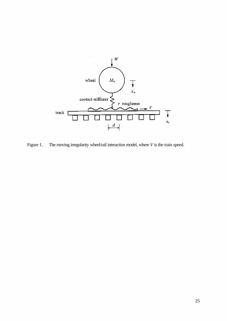
Figure 1 shows the form of the wheel/rail interaction. Here the moving irregularity model is used,
in which a roughness is pulled between a stationary wheel and the rail. In this system there are three
dynamic systems; the wheel and track are considered to be linear, while the contact stiffness is non-
linear. For simplicity the wheel is represented by a mass (its unsprung mass). As only higher
frequency vibration above 50 Hz is of interest here, the coupling with the vehicle vibration is ignored
because it is isolated by the soft suspension springs.
The force-deflection relation of the contact stiffness is assumed to follow the Hertz law and can
be given in the form

4
f C x x rH w r= − −( ) /3 2 (2)
where f is the wheel/rail contact force, xw and xr are the wheel and rail displacement respectively, r
is the roughness and CH is the Hertzian constant. This expression is exact for cylindrical surfaces,
which meet at an elliptical contact patch, and provides an approximation for other contact geometry.
The excitation, the roughness r, can be regarded as a broad band process from a practical point of
view, for example, the roughness wavelengths of relevance for rolling noise are typically in the range
5 mm to 0.5 m. At a train speed of 100 km/h (27.8 m/s) these wavelengths correspond to a
frequency range 55 − 5500 Hz, the shorter wavelengths applying to higher frequencies.
The track is the most complicated of the three sub-systems. Usually the vertical track dynamics
can be described in this frequency range by an infinite Timoshenko beam with continuous or discrete
spring-mass-spring supports representing railpad, sleeper and ballast, see reference [13]. However,
such a model brings great difficulties in calculations of the wheel/rail interaction with non-linearity. To
make the mathematical treatment easier, some simpler alternative models for track dynamics need to
be developed. Before doing this, a concise introduction of the track dynamic behaviour is given.
2.2. INTRODUCTION OF TRACK DYNAMICS
Track models are used to calculate the rail vibration and to determine the wheel/rail interaction
force. In terms of the wheel/rail vertical interaction up to about 5 kHz, cross-sectional deformations
of the rail that occur at high frequencies are not important and thus the rail can be well approximated
by a Timoshenko beam model. Two such models are commonly used [6, 13]: (a) an infinite rail
continuously supported by damped resilient and mass layers (railpads, sleepers and ballast); (b) an
infinite rail discretely supported by pad, sleeper and ballast. Using a track model with discrete
supports the so-called pinned-pinned resonance can be observed, in which the track receptance has

5
a maximum when the excitation acts between sleepers and a minimum when the excitation acts at a
sleeper. This occurs because the sleeper spacing is equal to half the wavelength of the flexural waves
at this frequency. Apart from the pinned-pinned resonance, the two track models have a similar
dynamic behaviour.
Figure 2 shows the point receptance of a typical track (displacement per unit force at the forcing
point) from a continuous model and a discrete model with the force acting at mid-span between
sleepers. The parameters for the track models are listed in Table 1. Three resonance peaks can be
seen, at about 80 Hz, 520 Hz and 1050 Hz. At 80 Hz the whole track bounces on the vertical
stiffness of the ballast, while at 520 Hz the rail vibrates on the pad stiffness, the latter frequency
depending on the pad stiffness. The sharp peak at 1050 Hz is the pinned-pinned resonance, which
can only be observed using a discretely supported track model. Detailed analysis of track dynamics
can be found in references [14, 15] and an extensive review of literature by Knothe and Grassie
[16].
2.3. EQUIVALENT MDOF TRACK MODEL
In order to allow for non-linear analysis of the wheel/rail interaction in the time-domain, an
equivalent multiple degree-of-freedom (MDOF) model for track dynamics is needed to represent an
infinite beam model. Nielson and Igeland [3] developed an MDOF model for a 22 m long track
section using the finite element method. To reduce the scale of the problem, a modal synthesis
technique was applied to the FE model (using only 185 modes).
Another possibility that can be considered is to approximate in a least-square sense a frequency
response function (receptance) from an existing infinite track model by a limited modal
decomposition. This approach was used by Fingberg [17]. A similar methodology is used here to

6
represent an infinite track model by an MDOF model that has approximately the same frequency
response function as the infinite track.
Firstly the frequency response function (point receptance curve) of an infinite track to be
approximated should be chosen. It is chosen here from the result of the continuously supported track
model given in Figure 2. This is because the pinned-pinned resonance phenomenon, due to the
infinite beam structure with periodic supports, has sharp peaks and troughs in both magnitude and
phase which cannot be well fitted by an MDOF system. On the other hand, in practice it has been
found that the pinned-pinned resonance may be cancelled or suppressed due to the wave reflections
from other wheels or due to the random sleeper spacing [18, 19]. Therefore the receptance curve
from the continuously supported track model can be used to take advantage of its simpler form
which is more amenable to be approximated by an equivalent MDOF system.
The second step is to find an equivalent system corresponding to the point receptance of the
infinite track. The system should have a transfer function expressed in the form of a ratio of two
polynomials, so that conventional system theory can be applied for setting up a mathematical model
in the time-domain. This is actually a curve fitting problem for which the function ‘invfreqs’ in the
Signal Processing Toolbox of MATLAB has been used. This function returns the real numerator and
denominator coefficient vectors b and a of the transfer function
H sB sA s
b s b s bs a s a
m mm
n nn
( )( )( )
......
= =+ + ++ + +
−+
−1 2
11
11 (3)
whose complex frequency response approximates the required frequency response at specified
frequency points. Scalars m and n specify the desired orders of the numerator and denominator
polynomials. More details about the algorithm of this function can be found in [20]. The most
important point for using this function is that whatever values of m and n are selected, it must be
ensured that all the poles of the returned transfer function H(s) are in the left half-plane and thus the
7
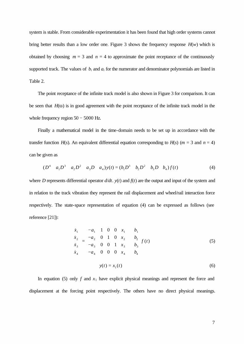
system is stable. From considerable experimentation it has been found that high order systems cannot
bring better results than a low order one. Figure 3 shows the frequency response H(ω) which is
obtained by choosing m = 3 and n = 4 to approximate the point receptance of the continuously
supported track. The values of bi and ai for the numerator and denominator polynomials are listed in
Table 2.
The point receptance of the infinite track model is also shown in Figure 3 for comparison. It can
be seen that H(ω) is in good agreement with the point receptance of the infinite track model in the
whole frequency region 50 − 5000 Hz.
Finally a mathematical model in the time-domain needs to be set up in accordance with the
transfer function H(s). An equivalent differential equation corresponding to H(s) (m = 3 and n = 4)
can be given as
( ) ( ) ( ) ( )D a D a D a D a y t b D b D b D b f t41
32
23 4 1
32
23 4+ + + + = + + + (4)
where D represents differential operator d/dt. y(t) and f(t) are the output and input of the system and
in relation to the track vibration they represent the rail displacement and wheel/rail interaction force
respectively. The state-space representation of equation (4) can be expressed as follows (see
reference [21]):
&&&&
( )
xxxx
aaaa
xxxx
bbbb
f t
1
2
3
4
1
2
3
4
1
2
3
4
1
2
3
4
1 0 00 1 00 0 10 0 0
=
−−−−
+
(5)
y t x t( ) ( )= 1 (6)
In equation (5) only f and x1 have explicit physical meanings and represent the force and
displacement at the forcing point respectively. The others have no direct physical meanings.

8
Nevertheless the system described by equation (5) has a similar frequency response function to that
of an infinite track and thus is an alternative representation for the track model.
2.4. EQUATION OF WHEEL/RAIL INTERACTION
Referring to Figure 1, the equation of motion for the wheel/rail interaction and the wheel and rail
vibration can be written as follows, using the equivalent MDOF model for the track dynamics:
&&&&
xxxx
aaaa
xxxx
bbbb
f
1
2
3
4
1
2
3
4
1
2
3
4
1
2
3
4
1 0 00 1 00 0 10 0 0
=
−−−−
+
(7a)
&& ( )x xx W f Mw
5 6
6
== −
(7b)
fC x x r x x r
x x rH=
− − − − >
− − ≤
( ) ,
,
/5 1
3 25 1
5 10
0
0 (7c)
where x5 = xw is the wheel displacement, x1 = xr is the rail displacement, W is the static load at one
wheel from the weight of the vehicle, Mw is the wheel mass (unsprung mass), f is the non-linear
wheel/rail interaction force, CH is the Hertzian constant and r is the roughness excitation. Equations
(7) can be solved numerically using the Runge-Kutta method.
3. WHEEL/RAIL INTERACTION DUE TO A HARMONIC ROUGHNESS
3.1. CASES CONSIDERED
In this section the wheel/rail interaction and vibration are investigated using a single harmonic
roughness input at various frequency points in the region 50 − 5000 Hz. In this way the effects on the
wheel/rail interaction of the non-linear contact can be examined at each frequency considered. This is
useful because the wheel/rail interaction is determined by the dynamic response of three components:
9
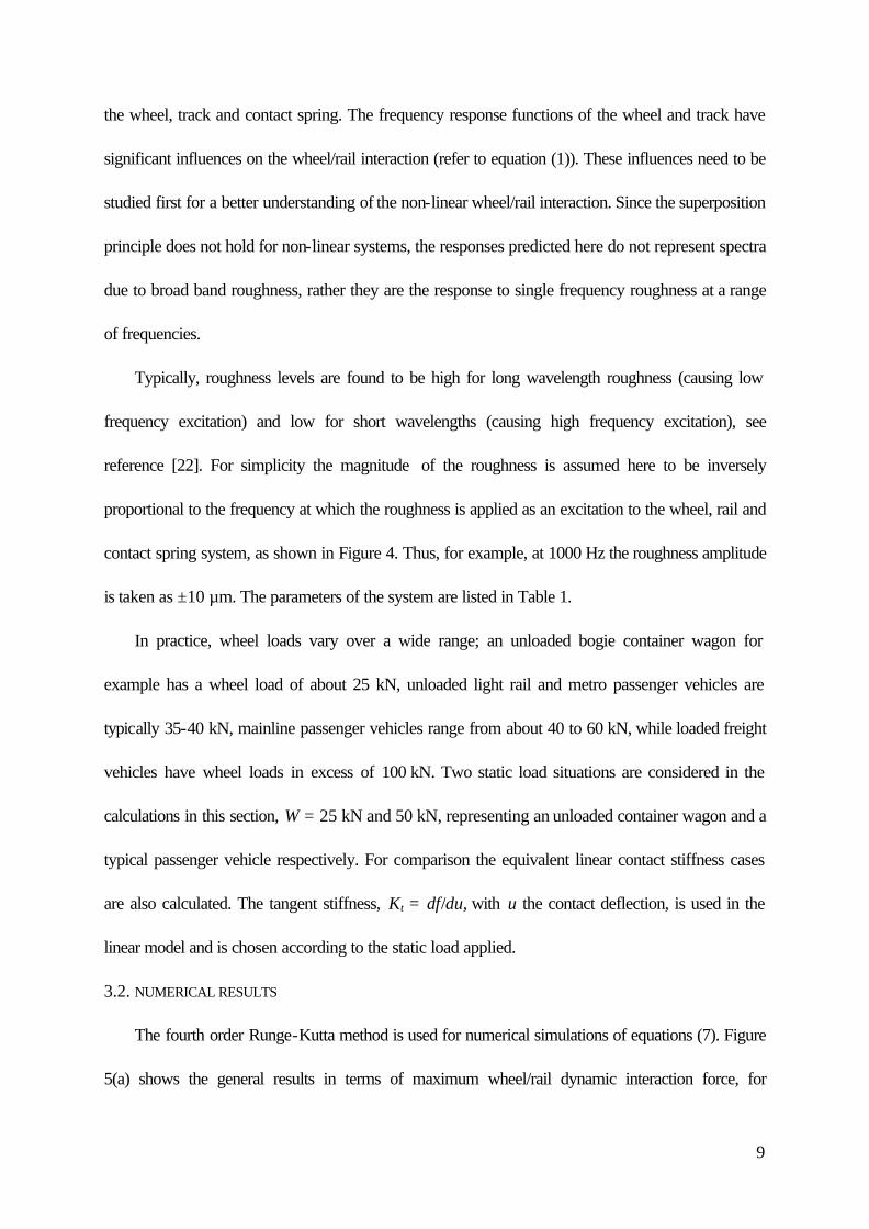
the wheel, track and contact spring. The frequency response functions of the wheel and track have
significant influences on the wheel/rail interaction (refer to equation (1)). These influences need to be
studied first for a better understanding of the non-linear wheel/rail interaction. Since the superposition
principle does not hold for non-linear systems, the responses predicted here do not represent spectra
due to broad band roughness, rather they are the response to single frequency roughness at a range
of frequencies.
Typically, roughness levels are found to be high for long wavelength roughness (causing low
frequency excitation) and low for short wavelengths (causing high frequency excitation), see
reference [22]. For simplicity the magnitude of the roughness is assumed here to be inversely
proportional to the frequency at which the roughness is applied as an excitation to the wheel, rail and
contact spring system, as shown in Figure 4. Thus, for example, at 1000 Hz the roughness amplitude
is taken as ±10 µm. The parameters of the system are listed in Table 1.
In practice, wheel loads vary over a wide range; an unloaded bogie container wagon for
example has a wheel load of about 25 kN, unloaded light rail and metro passenger vehicles are
typically 35-40 kN, mainline passenger vehicles range from about 40 to 60 kN, while loaded freight
vehicles have wheel loads in excess of 100 kN. Two static load situations are considered in the
calculations in this section, W = 25 kN and 50 kN, representing an unloaded container wagon and a
typical passenger vehicle respectively. For comparison the equivalent linear contact stiffness cases
are also calculated. The tangent stiffness, Kt = df/du, with u the contact deflection, is used in the
linear model and is chosen according to the static load applied.
3.2. NUMERICAL RESULTS
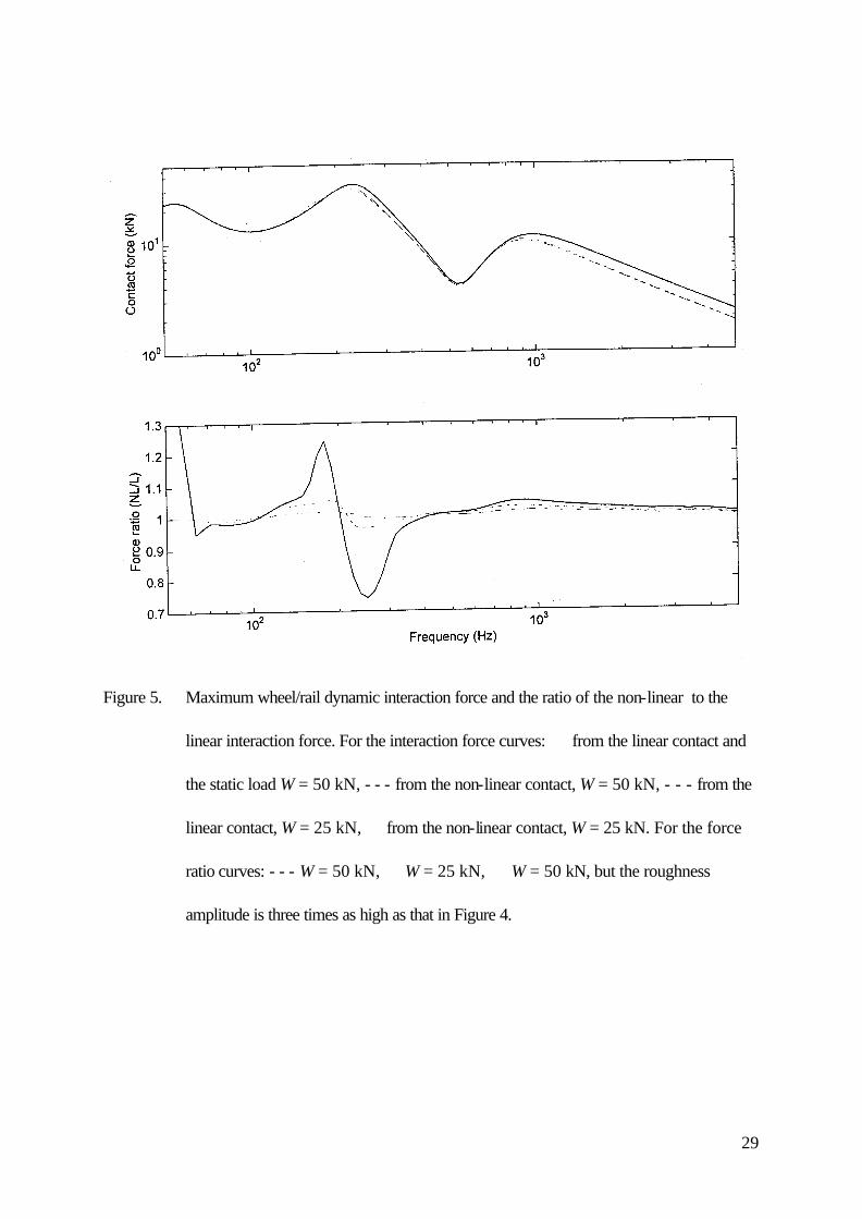
The fourth order Runge-Kutta method is used for numerical simulations of equations (7). Figure
5(a) shows the general results in terms of maximum wheel/rail dynamic interaction force, for
10
frequencies in the region 50 − 5000 Hz, due to the roughness excitation amplitude shown in Figure 4.
This maximum dynamic force is obtained by subtracting the static load from the peak contact force.
The results from equivalent linear cases (using equation (1)) are also presented in Figure 5(a).
The interaction force can be seen to vary with frequency in a manner which follows the inverse
of the track receptance (Figure 3) for frequencies up to 900 Hz. Compared with the linear case, the
non-linear effects due to the roughness input shown in Figure 4 are only noticeable in the frequency
region around 200 Hz and 900 Hz and only for the lighter static load. The ratio of the non-linear
wheel/rail interaction force to the linear one is shown in Figure 5(b). This shows that the greatest
difference between the two cases is only five percent. Slight loss of contact between the wheel and
rail occurs for excitation at about 200 − 250 Hz, but it does not affect the magnitude of the
interaction force greatly.
A larger roughness input is also considered of three times that given in Figure 4. In this case the
non-linear effects are significant, as seen in Figure 5(b), because of severe loss of contact between
the wheel and rail. Loss of contact occurs for excitation at low frequencies up to 70 Hz and from
150 to 300 Hz due to the very large roughness amplitudes.
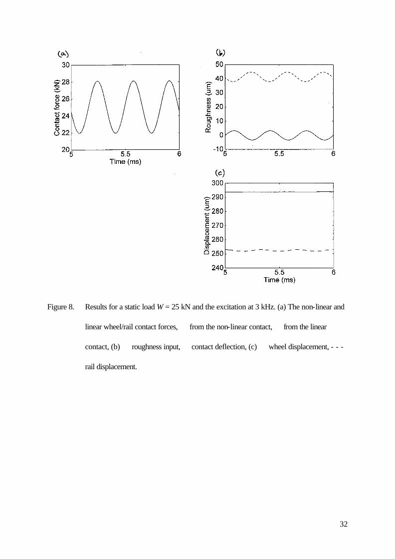
Figures 6 − 8 show examples of the non-linear contact forces and the vibrations of the wheel
and track in the time-domain at 180 Hz, 1 kHz and 3 kHz respectively. These results are for an
arbitrary time period once steady state has been reached in each case. From Figure 6(a), compared
with the linear interaction, the effects of the non-linearity at 180 Hz can be identified. The half-period
when the contact force is greater than the static load can be observed to be slightly shorter than the
other half-period in which the contact force is below the static load. Thus some super-harmonic
components are generated in the responses of the system, although their magnitudes are very small.

11
This is shown in Figure 6(b). For example the component at 360 Hz has an amplitude of about 5%
of the 180 Hz component.
Comparing the three cases in Figures 6 − 8, both the wheel and the rail responses are large at
180 Hz, whereas the wheel response is very small at 1 kHz and the rail response is also small at 3
kHz. Moreover the wheel is almost stationary at 3 kHz. The wheel/rail interaction is therefore
determined by the contact spring, wheel and track at 180 Hz, by the contact spring and track at 1
kHz and by the contact spring alone at 3 kHz.
3.3. ANALYSIS OF THE NON-LINEAR EFFECTS
Although the effects of non-linearity are found to be limited according to the numerical
simulations when the roughness input is not large, a detailed analysis of how the non-linear contact
affects the wheel/rail interaction is helpful. The analysis here is carried out both from aspects of the
non-linearity of the contact stiffness and the dynamic properties of the wheel and track.
Figure 9(a) shows the force-deflection curve of the non-linear contact spring. Using Taylor
series the non-linear contact force-deflection relation can be written as
f u f udf u
duu u
d f udu
u u( ) ( )
( )( )
( ) ( )!
= + − +−
+00
0
20
20
2
2LL (8)
where u is the contact deflection and u0 is the deflection under a certain static load. Thus f(u0)
represents the static load W and df u du( )0 is the tangent stiffness Kt under this static load. Two
tangents are shown in Figure 9(a) at the load points W = 25 kN and 50 kN. They are equal to the
first two terms (linear terms) from the right-hand side in equation (8) and represent the equivalent
linear contact stiffness under the load considered. The differences between the linear and non-linear
contact can be observed in Figure 9(b) in terms of the ratio of the non-linear contact force to the
linear one. For a given deflection, the non-linear contact force can be seen to be closer to the linear
12
one if a greater static load is applied. Thus it is clear that the influence of the non-linear contact is
weaker when the static load is greater. This is observed in the results of Figure 5(b).
In addition the deviations between the non-linear and linear contact forces in Figure 9(b)
increase with increasing contact deflection. The magnitude of the contact deflection is determined by
both the roughness level and the dynamic behaviour of the wheel and track. Therefore it can be
expected that the extent of non-linear effects is also affected by the dynamic properties of the wheel
and track.
Figure 10(a) shows the receptances of the wheel, track and the equivalent tangent contact
stiffness under the static load of 25 kN and 50 kN in the frequency region 50 − 5000 Hz. Figure
10(b) indicates the ratio of the dynamic contact deflection to the roughness input. It can be seen from
Figure 10(a) that the wheel and track receptances are much greater than that of the contact stiffness
at low frequencies so that the contact spring here can be regarded as effectively rigid. Because of this
the ratio of the contact deflection to the roughness (Figure 10(b)) is very small at low frequencies.
Thus the large roughness input at low frequencies only results in small contact deflection. The
wheel/rail interactions therefore are almost the same whether they are based on the linear or non-
linear model as long as loss of contact does not occur. If severe loss of contact occurs due to a very
large roughness input, however, the non-linear contact force is larger than the linear one since the
non-linear contact spring becomes stiffer with increasing deflection. Such results are found in Figure
5(b).
Around 200 Hz and 900 Hz the receptances of the wheel, track and contact spring are similar in
magnitude. Moreover, around 200 Hz the roughness level is still high and the ratio of the contact
deflection to the roughness rises to about 0.6, whilst around 900 Hz this ratio is close to 1, although
the roughness level assumed here is not as high as at 200 Hz. As a result, in both cases the contact

13
deflection is relatively large and the non-linear contact becomes important. This explains why the
non-linear effects are most noticeable around 200 Hz and, to a lesser extent, 900 Hz in Figure 5.
As both the wheel and the track receptances are much smaller than that of the contact spring at
high frequencies, the contact deflection is virtually equal to the roughness above 1 kHz. This might
suggest that the non-linear contact would now dominate. On the other hand, however, the roughness
magnitude at short wavelength is fairly low in practice. As a result, the effects of the non-linearity are
very limited because of the small dynamic contact deflection. As the ratio of the contact deflection to
the roughness input is quite stable above 1 kHz and slightly higher than 1, the effects of non-linear
contact are here determined purely by the roughness magnitude for a given static contact load.
The above analysis is based on the condition that no loss of contact occurs between the wheel
and rail. When loss of contact occurs due to large roughness input, the difference in the contact
forces between linear and non-linear models can be large, as shown in Figure 5(b). This is because
the wheel and rail are bound to remain in contact in the linear model.
4. WHEEL/RAIL INTERACTION DUE TO A BROAD BAND RANDOM ROUGHNESS
4.1. RANDOM ROUGHNESS INPUT
So far, sinusoidal roughness at different frequencies has been considered. In practice, the
roughness excitation is composed of unevenness on the wheel and rail contact surfaces having a
broad band spectrum over a range of wavelengths. When a train runs on the rails, the unevenness
forms an excitation with multiple frequency components which can be regarded as a broad band
random process. On the other hand, since a non-linear contact stiffness is taken account of in the
wheel/rail interaction model, the superposition principle does not hold here and frequency-domain
analysis according to equation (1) cannot be performed. A practical roughness input is therefore

14
needed to simulate the wheel/rail interaction and the responses of the wheel and track in the time-
domain.
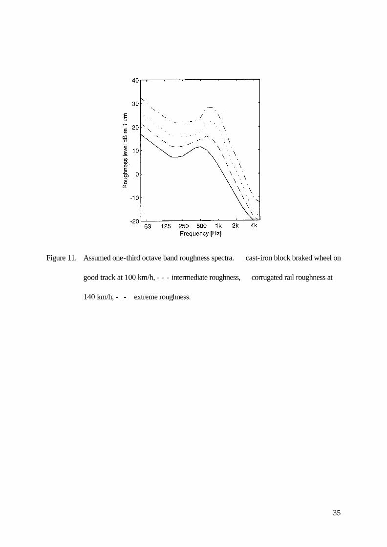
Figure 11 shows four one-third octave band roughness spectra. The solid line corresponds to
the roughness of a wheel with cast-iron block brakes on good quality track at 100 km/h, while the
dotted line corresponds to corrugated track at 140 km/h [23]. Two other spectra are also shown: an
intermediate roughness which is the geometric mean of the above two spectra, and an extreme
roughness which has twice the amplitude of the corrugated rail spectrum. Summing these spectra for
the frequency bands 250 Hz and above, the r.m.s. amplitudes of the roughness are found to be 7.6,
13.2, 25 and 50 µm.
Starting from each of these spectra, a narrow-band spectrum is generated, with a bandwidth of
5 Hz, which corresponds to the one-third octave band spectrum. For simplicity, this contains equal
energy in each narrow band within a given 1/3 octave band. Below 50 Hz the magnitude of the
spectrum is set to 0.
This narrow-band spectrum is then used to generate a time series by using the inverse Fourier
transform, the phase of each Fourier component being chosen randomly between −π and π . This
time series is used as the roughness input to the wheel/rail system.
4.2. RESULTS FOR RANDOM ROUGHNESS EXCITATION
Numerical simulations are carried out using equation (7) and a random roughness input which is
constructed as described above. Results for the corrugated track roughness are presented in Figure
12, in terms of the non-linear contact force, contact deflection and displacements of the wheel and
rail in the time-domain. The roughness input is also shown. The static load W here is chosen as
25 kN, corresponding to unloaded container wagons.
15
From Figure 12 the variations in the wheel/rail contact force can be seen to be very sharp. A
sharp peak of the contact force appears when a sharp negative roughness input is applied. (The sign
convention adopted for roughness is positive for a dip, negative for an asperity.) Some peaks in the
contact force are as great as three times the static load, but complete unloading is rare. The wheel
and rail displacements generally follow the roughness input, although the wheel cannot follow the high
frequency components of the input due to its large inertia. Loss of contact or sharp peaks of the
contact force are induced at large roughness dips or asperities. It can be observed from Figure 12
that the low frequency components in the rail response are delayed compared with the roughness
input, whereas the high frequency components are out of phase with the input.
Because of the wheel and rail response properties, the dynamic contact deflection in Figure 12
can be seen to be much smaller than the roughness input and to consist mainly of high frequency
components. As a result, the effects of the non-linear contact stiffness are not expected to be very
noticeable provided loss of contact does not occur.
Figure 13 shows one-third octave band spectra of the wheel/rail dynamic interaction forces,
from both the linear and the non-linear models, for the corrugated track and for a range of wheel
static loads.
For the higher static loads, only small differences between the two models are found. For small
values of load the contact force spectra decrease. The results from the non-linear model decrease
more than those from the linear model around 250 and 800 Hz and do not appear to decrease for
frequencies above 2 kHz. For a 50 kN static load, typical of passenger vehicles, it is found that non-
linear interactions modify the force spectrum by at most 2 dB (in the 2 kHz band); for a 25 kN static
load this maximum difference increases to 4 dB. Note that the preloads less than 25 kN are included
to demonstrate the trends although they are unrealistically small for most situations.

16
Figure 14 shows the difference between the interaction force spectra predicted using non-linear
and linear models for each load case. As well as the results for the corrugated track roughness
shown in Figure 13, this also shows results for the other roughness spectra of Figure 11.
For the smoothest situation considered, the differences are all less than 0.5 dB, indicating that a
linear model is adequate for this case. At the intermediate level of roughness, the linear model only
gives significantly different results from the non-linear model for the lowest static load considered (10
kN), which is much less than normal values. As the roughness amplitude increases, however, the
inadequacy of the linear model also becomes apparent at higher values of static load, as might be
expected from the results of the previous section. Thus for the corrugated rail roughness the non-
linear model is required for wheel loads of up to 35 kN, and for the extreme roughness for loads up
to 70 kN.
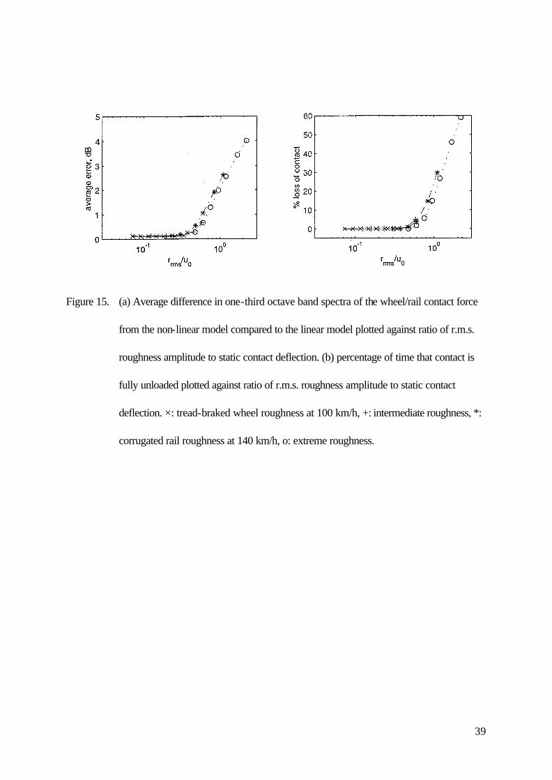
In order to summarise these results, the mean is formed over all one-third octave frequency
bands from 50 to 5000 Hz of the absolute differences in level given in Figure 14. This gives a single
measure of the deviation between linear and non-linear models for the seven wheel loads and four
roughness spectra considered. These results are plotted in Figure 15(a) against the ratio of the r.m.s.
roughness amplitude (for 250 Hz and above) to the static deflection in the contact zone, u0. The
results for the four roughness spectra follow a similar trend. These results indicate that the difference
between linear and non-linear models is negligible where the r.m.s. roughness amplitude is less than
about 0.35 times the static contact deflection, and rapidly becomes significant above this.
In Figure 15(b) the percentage of the time that the wheel loses contact with the rail is plotted for
each of the simulations. At low roughness no loss of contact occurs; the loss of contact rises to as
much as 60% of the time for the extreme roughness spectrum and 10 kN load. These curves show
similar trends to the deviations between linear and non-linear models in Figure 15(a). However, it is

17
found that loss of contact is only significant for r.m.s. roughness amplitudes above about 0.5 times
the static contact deflection. Thus non-linear effects become important slightly before significant loss
of contact occurs.
5. CONCLUSIONS
The effects of the non-linear contact on the wheel/rail dynamic interaction have been investigated
through numerical simulations, analysis and comparisons with the results from the linear contact
model. A simplified MDOF model equivalent to an infinite track has been developed, which has
approximately the same frequency response function as the infinite track in the frequency region 50 −
5000 Hz. Using this equivalent track model a non-linear wheel/rail interaction model has been set up
in state-space form for numerical simulations. The wheel/rail interaction has been investigated using
both a single harmonic roughness excitation and a broad band random roughness input. The results
are compared with those from the linear contact to check the effects of the non-linear contact. These
effects are also analysed from the aspects of the non-linear contact force-deflection relationship and
the dynamic behaviour of the wheel and track.
It has been found that the effects of the non-linear contact on the wheel/rail interaction are
affected by the static preload and the dynamic properties of the wheel and rail. Under a large static
contact load the non-linear effects on the wheel/rail dynamic interaction and vibration are weak and
can be ignored. This is because the difference between the non-linear stiffness and the equivalent
linear (tangent) stiffness is very small for a large static preload. The non-linear effects on the
wheel/rail interaction are also not noticeable at low frequencies up to 100 Hz because in this
frequency region the wheel and rail dynamic stiffness is much less than the contact stiffness and thus
the latter can be regarded as effectively rigid, so that the question of its linearity is unimportant here.

18
From a practical point of view, the non-linear effects are also not noticeable at high frequencies
(above 1 kHz) because the roughness level at short wavelengths is generally very low. In such a case
the dynamic contact deflection is small and the non-linear contact force-deflection relation can be
well approximated by a linear one. The non-linear effects are only noticeable when the roughness
excitation is in the frequency region around 200 Hz and 900 Hz, where the dynamic stiffness of the
wheel and rail is similar to the contact stiffness, but even so the difference between the non-linear and
linear interactions is very limited.
The difference is also small when a typical broad band random roughness excitation is applied.
In the examples considered, if the wheel and rail surfaces are in good condition (r.m.s. amplitudes of
roughness below 15 µm), the linear model can be used without significant error for all static loads
down to 25 kN (equivalent to an unloaded container wagon). When the track is corrugated with an
r.m.s. amplitude of 25 µm, good agreement between linear and non-linear models is obtained for
static loads of 50 kN and above, but agreement is less good for lower loads. Non-linear interactions
modify the force spectrum by at most 2 dB for 50 kN; for 25 kN this increases to 4 dB.
When loss of contact occurs due to large roughness and lighter static load, the differences
between linear and non-linear models become more significant. This is because the wheel and rail are
bound to remain in contact in the linear model. In fact differences between the linear and non-linear
models occur at slightly lower roughness amplitudes than those which induce significant loss of
contact.
All the above suggests that the non-linear wheel/rail dynamic interaction model can be well
approximated using an equivalent linear model when the roughness level is not extremely severe and
a moderate static preload is applied to keep the wheel and rail in contact. Since a linear model can
be expressed in the frequency domain, use of such a model greatly simplifies calculations.

19
ACKNOWLEDGEMENTS
The work described has been performed within the project ‘Non-linear Effects at the Wheel/rail
Interface and their Influence on Noise Generation’ funded by EPSRC (Engineering and Physical
Sciences Research Council of the United Kingdom), grant GR/M82455.
20
REFERENCES
1. B. Ripke 1995 Fortschritt-Berichte VDI Reihe 12, Nr. 249. Hochfrequente Gleismodellierung
und Simulation der Fahrzeug-Gleis-Dynamik unter Verwendung einer nichtlienearen
Kontaktmechanik.
2. Z. Sibaei 1992 Fortschritt-Berichte VDI Reihe 11, Nr. 165. Vertikale Gleisdynamik beim
Abrollen eines Radsatzes - Behandlung im Frequenzbereich.
3. J. C. O. Nielson and A. Igeland 1995 Journal of Sound and Vibration 187, 825-839. Vertical
dynamic interaction between train and trackinfluence of wheel and track imperfections.
4. L. Frýba 1988 ILR-Bericht 58, 9-38. Dynamics of rail and track.
5. P. J. Remington 1987 J. Acoust. Soc. Am. 81, 1805-1823. Wheel/rail rolling noise I: theoretical
analysis.
6. S. L. Grassie, R. W. Gregory, D. Harrison and K. L. Johnson 1982 Journal Mechanical
Engineering Science 24, 77-90. The dynamic response of railway track to high frequency
vertical excitation.
7. D. J. Thompson 1993 Journal of Sound and Vibration 161, 387-400. Wheel-rail noise
generation, part I: introduction and interaction model.
8. H. Hertz 1882 Journal für die rein und angewandte Mathematik 92, 156-171. Über die
Berührung fester elastischer Körper.
9. S. G. Newton and R. A. Clark 1979 Journal Mechanical Engineering Science 21, 287-297.
An investigation into the dynamic effects on the track of wheelflats on railway vehicles.
10. R. A. Clark, P. A. Dean, J. A. Elkins and S. G. Newton 1982 Journal Mechanical
Engineering Science 24, 65-76. An investigation into dynamic effects of railway vehicles
running on corrugated rails.

21
11. A. Igeland 1996 Proc. Instn. Mech. Engrs. Part F 210, 11-20. Railhead corrugation growth
explained by dynamic interaction between track and bogie wheelsets.
12. H. Ilias and K. Knothe 1992 Fortschritt-Berichte VDI Reihe 12, Nr. 177. Ein diskret-
kontinuierliches Gleismodell unter dem Einfluß schnell bewegter, harmonisch schwankener
Wanderlasten.
13. D. J. Thompson and N. Vincent 1995 Vehicle System Dynamics Supplement 24, 86-99. Track
dynamic behaviour at high frequencies. Part 1: Theoretical models and laboratory measurements.
14. T. X. Wu and D. J. Thompson 1999 Journal of Sound and Vibration 224, 329-348. A double
Timoshenko beam model for vertical vibration analysis of railway track at high frequencies.
15. N. Vincent and D. J. Thompson 1995 Vehicle System Dynamics Supplement 24, 100-114.
Track dynamic behaviour at high frequencies. Part 2: Experimental results and comparisons with
theory.
16. KL. Knothe and S. L. Grassie 1993 Vehicle System Dynamics 22, 209-262. Modelling of
railway track and vehicle/track interaction at high frequencies.
17. U. Fingberg 1990 Journal of Sound and Vibration 143, 365-377. A model of wheel-rail
squealing noise.
18. T. X. Wu and D. J. Thompson 2000 Acta Acustica 86, (in press). The influence of random
sleeper spacing and ballast stiffness on the vibration behaviour of railway track.
19. T. X. Wu and D. J. Thompson 1999 Proceedings of Sixth International Congress on Sound
and Vibration, Lyngby, Denmark, 2629-2636. Effects of multiple wheels on a rail on the rail
vibration.
20. T. P. Krauss, L. Shure and J. N. Little 1994 Signal Processing Toolbox User’s Guide. The
Math Works Inc.

22
21. F. H. Raven 1978 Automatic Control Engineering. Tokyo: McGraw-Hill; third edition.
22. D. J. Thompson 1996 Journal of Sound and Vibration 193, 149-160. On the relationship
between wheel and rail surface roughness and rolling noise.
23. P.C. Dings, M.G. Dittrich 1996 Journal of Sound and Vibration 193, 103-112. Roughness on
Dutch railway wheels and rails.
23
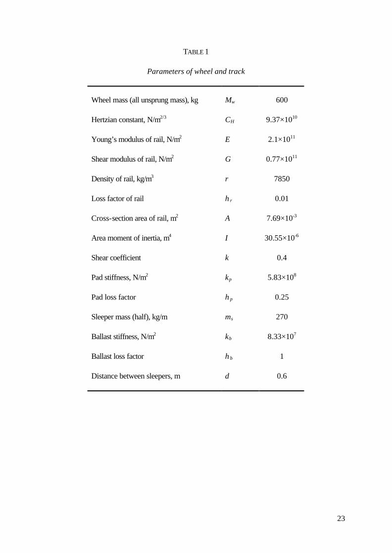
TABLE 1
Parameters of wheel and track
Wheel mass (all unsprung mass), kg Mw 600
Hertzian constant, N/m2/3 CH 9.37×10¹⁰
Young’s modulus of rail, N/m2 E 2.1×10¹¹
Shear modulus of rail, N/m2 G 0.77×10¹¹
Density of rail, kg/m3 ρ 7850
Loss factor of rail ηr 0.01
Cross-section area of rail, m2 A 7.69×10⁻³
Area moment of inertia, m4 I 30.55×10⁻⁶
Shear coefficient κ 0.4
Pad stiffness, N/m2 kp 5.83×10⁸
Pad loss factor ηp 0.25
Sleeper mass (half), kg/m ms 270
Ballast stiffness, N/m2 kb 8.33×10⁷
Ballast loss factor ηb 1
Distance between sleepers, m d 0.6

24
TABLE 2
Parameters of MDOF track model
a1 1.77 × 10³ b1 3.28 × 10⁻⁶
a2 1.26 × 10⁷ b2 1.87 × 10⁻²
a3 7.87 × 10⁹ b3 23.6
a4 3.93 × 10¹² b4 3.97 × 10⁴
25
Figure 1. The moving irregularity wheel/rail interaction model, where V is the train speed.

26
Figure 2. Magnitude and phase of the point receptance of an infinite track. from the
continuously supported track model, ⋅⋅⋅⋅⋅ from the discretely supported track model with
force at mid-span.

27
Figure 3. Magnitude and phase of the frequency response function. from the infinite
continuously supported track, ⋅⋅⋅⋅⋅ from the equivalent MDOF model.

28
Figure 4. Assumed roughness amplitude for single frequency excitation.
29
Figure 5. Maximum wheel/rail dynamic interaction force and the ratio of the non-linear to the
linear interaction force. For the interaction force curves: from the linear contact and
the static load W = 50 kN, -⋅-⋅- from the non-linear contact, W = 50 kN, - - - from the
linear contact, W = 25 kN, ⋅⋅⋅⋅⋅ from the non-linear contact, W = 25 kN. For the force
ratio curves: -⋅-⋅- W = 50 kN, ⋅⋅⋅⋅⋅ W = 25 kN, W = 50 kN, but the roughness
amplitude is three times as high as that in Figure 4.

30
Figure 6. Wheel/rail interaction results for a static load W = 25 kN and excitation at 180 Hz. (a)
The non-linear and linear wheel/rail contact forces, from the non-linear contact, ⋅⋅⋅⋅⋅
from the linear contact, (b) frequency components of the non-linear contact force, (c)
roughness input, ⋅⋅⋅⋅⋅ contact deflection, (d) wheel displacement, - - - rail
displacement.

31
Figure 7. Results for a static load W = 25 kN and the excitation at 1 kHz. (a) The non-linear and
linear wheel/rail contact forces, from the non-linear contact, ⋅⋅⋅⋅⋅ from the linear
contact, (b) roughness input, ⋅⋅⋅⋅⋅ contact deflection, (c) wheel displacement, - - -
rail displacement.
32
Figure 8. Results for a static load W = 25 kN and the excitation at 3 kHz. (a) The non-linear and
linear wheel/rail contact forces, from the non-linear contact, ⋅⋅⋅⋅⋅ from the linear
contact, (b) roughness input, ⋅⋅⋅⋅⋅ contact deflection, (c) wheel displacement, - - -
rail displacement.

33
Figure 9. (a) Non-linear contact force-deflection relation, (b) ratios of the non-linear contact force
to the equivalent linear contact force. -⋅-⋅- the static load W = 25 kN, ⋅⋅⋅⋅⋅ the static load
W = 50 kN.

34
Figure 10. (a) Receptances of the wheel, track and the equivalent tangent contact stiffness.
rail receptance, ⋅⋅⋅⋅⋅ wheel receptance, - - - receptance of tangent stiffness under
static load 50 kN, -⋅-⋅- receptance of tangent stiffness under static load 25 kN.
(b) Ratio of the amplitude of the dynamic contact deflection to the roughness input, the
static load W = 50 kN. from the linear contact, ⋅⋅⋅⋅⋅ from the non-linear contact.
35
Figure 11. Assumed one-third octave band roughness spectra. cast-iron block braked wheel on
good track at 100 km/h, - - - intermediate roughness, ⋅⋅⋅⋅⋅ corrugated rail roughness at
140 km/h, - ⋅ - ⋅ extreme roughness.

36
Figure 12. The non-linear wheel/rail contact force, broad band random roughness input (from
corrugated track, spectrum from Figure 11) and the wheel and rail displacements, the
static load W = 25 kN. (a) contact force, (b) roughness input, ⋅⋅⋅⋅⋅ contact deflection,
(c) wheel displacement, - - - rail displacement.

37
Figure 13. One-third octave band spectra of the wheel/rail contact force for corrugated track
roughness, (a) from the linear model, (b) from the non-linear model. From bottom to
top, static load W = 10, 15, 25, 35, 50, 70, 100 kN.

38
Figure 14. Difference in one-third octave band spectra of the wheel/rail contact force from the non-
linear model compared to the linear model. From largest deviations to smallest, static
load W = 10, 15, 25, 35, 50, 70, 100 kN. (a) tread-braked wheel roughness at 100
km/h, (b) intermediate roughness, (c) corrugated rail roughness at 140 km/h, (d)
extreme roughness (amplitude doubled from (c)).
39
Figure 15. (a) Average difference in one-third octave band spectra of the wheel/rail contact force
from the non-linear model compared to the linear model plotted against ratio of r.m.s.
roughness amplitude to static contact deflection. (b) percentage of time that contact is
fully unloaded plotted against ratio of r.m.s. roughness amplitude to static contact
deflection. ×: tread-braked wheel roughness at 100 km/h, +: intermediate roughness, *:
corrugated rail roughness at 140 km/h, o: extreme roughness.