UCD GEARY INSTITUTE

DISCUSSION PAPER SERIES

Multidimensional Poverty Measurement in Europe: An

Application of the Adjusted Headcount Approach

Christopher T. Whelan

School of Sociology and Geary Institute, University College Dublin

Brian Nolan

College of Human Sciences, University College Dublin

Bertrand Maître Economic and Social Research Institute, Dublin

Geary WP2012/11 April 2012

UCD Geary Institute Discussion Papers often represent preliminary work and are circulated to encourage discussion. Citation of such a paper should account for its provisional character. A revised version may be available directly from the author.

Any opinions expressed here are those of the author(s) and not those of UCD Geary Institute. Research published in this series may include views on policy, but the institute itself takes no institutional policy positions.

Multidimensional Poverty Measurement in Europe: An Application of

the Adjusted Headcount Approach

Christopher, T. Whelan*, Brian Nolan** and Bertrand Maître***

*School of Sociology and Geary Institute, University College Dublin,

** College of Human Sciences, University College Dublin,

*** Economic and Social Research Institute, Dublin

Corresponding author

Christopher T. Whelan

Room B117 Geary Institute

University College Dublin

Belfield

Dublin 4

Ireland

e-mail: christopher.whelan@ucd.ie

phone: 00353 1 7164658

Multidimensional Poverty Measurement in Europe: An Application of

the Adjusted Headcount Approach

Abstract

As awareness of the limitations of relying solely on income to measure poverty and social

exclusion has become more widespread, attention has been increasingly focused on multi-

dimensional approaches. To date efforts to measure multidimensional poverty and social

exclusion in rich countries have been predominantly ad hoc and have relied on data that are

far from ideal. Here we apply the approach recently developed by Alkire and Foster,

characterized by a range of desirable axiomatic properties but mostly discussed so far in a

development context, to European countries, exploiting the potential of harmonized

microdata on deprivation newly available for the European Union. The analysis seeks to

overcome the limitations of the union and intersection approaches that have characterized

many earlier studies. Multidimensional poverty is characterized and decomposed in terms of

the contribution of different deprivation dimensions, and an account of cross-national and

socio-economic variation in risk levels is presented that is in line with theoretical

expectations. Multilevel analysis of multi-dimensional poverty provides the basis for

assessment of the role of macro and micro characteristics and their interaction in relation to

levels and patterns of multidimensional poverty and social exclusion.

Key words: Poverty Measurement; Multidimensional poverty; Deprivation; Social exclusion; EU poverty target.

3

Introduction

In developed as well as developing countries, attention has been increasingly focused on

multi-dimensional approaches to measuring poverty and social exclusion, identified by

Kakwani and Silber (21) as the most important recent development in poverty research. Non-

monetary indicators are increasingly available and used in this context, either separately or in

combination with income, in individual OECD countries as well as at the European Union

level Nolan and Whelan (25, 26), Förster(13). A variety of sophisticated analytic strategies

have been employed in individual countries to explore such issues, including latent class

analysis (Dewilde, (10) Moisio (24), Grusky and Weeden (16)), Whelan and Maître (35),

structural equation modelling (Carle et al (9), Tomlinson at al (31), item response theory

Capellari and Jenkins (8)) and self-organising maps Pisati et al (27). There have also been

comparative applications drawing on EU-wide survey micro-data, despite limitations in the

dimensions covered by available indicators to date ((Fusco et al (15), Nolan and Whelan

(26)). Debate on methodological approaches has been vigorous, focusing inter alia on the

value of summary indices for communication to a wide audience versus the arbitrary nature

of decisions required in combining distinct dimensions in producing such indices. Here we

apply the multidimensional poverty measurement approach recently developed by Alkire and

Foster (1,2,3) which has been the subject of considerable attention and debate (see for

example Lustig (23), Ravallion (28), Thorbecke (30)). This approach has been framed more

in a development context than a rich country one. Here we seek to apply it to the countries of

the European Union making use of newly-available and richer comparative data on various

aspects of deprivation. Our results bring out the relevance of this approach in such a context,

and help to illuminate on-going debates about the measurement and targeting of poverty and

social exclusion in Europe.

4

The Alkire and Foster Multidimensional Approach

Bourguignon and Chakravarty (7) provide a framework for multidimensional poverty

measurement involving both an identification function for counting the number poor and a

poverty measure that combines that information into a statistic summarizing the overall

extent of poverty. Axioms analogous to the ones used in the unidimensional case ensure that

the measure properly reflects poverty, can be decomposed by sub-group and is consistent

with the identification function. The simplest summary measure is the number of dimension

on which an individual or household is deprived, which Atkinson (6) refers to as the

‘counting’ approach. Atkinson (6) distinguishes between the union and intersection

approaches, the former counting as poor those deprived on any dimension while the latter

counting only those deprived on all dimensions. As Alkire and Foster (4) note, while the

union and intersection approaches are easy to understand, they can be particularly ineffective

at separating the poor from the non-poor, with the former tending to identify implausibly

large numbers as poor and the later tending to capture tiny minorities.

A key motivation underlying the recent methodological contributions of Alkire and Foster

(1,2,3), with concrete applications in a development context by Alkire and Santos (4) and

Alkire and Seth (5), is to address these shortcomings. Their procedure involves a dual cutoff

approach. Given a vector z= (z1,……...zj) of deprivation cutoffs, one for each dimension, if a

person’s outcome on a given deprivation dimension j falls short of the appropriate threshold

zj then the person is said deprived on that dimension. A vector of weights w= (w1,………….wj) is

used to indicate the relative importance of different dimensions; if each deprivation is viewed

as having equal importance, all weights are one and sum to the number of dimensions. A

column vector c= (c1, ………..cj) of deprivation counts reflects the breadth of each person’s

deprivation. In the case of equal weights, the i th person’s deprivation count is simply the

number of deprivations s/he experiences; more generally, it is the sum of the weighted values

5

of the deprivations experienced by i. A cutoff point 0 < k ≤ d is used to determine whether a

person has sufficient deprivations to be considered poor. If an individual’s deprivation count

is k or above the person is identified as poor.

Following Alkire and Foster (3), the transition between the identification and the aggregation

steps is best understood as involving a progression of matrices. The achievement matrix Y

shows the outcomes of n persons in each of d dimensions. The deprivation matrix gO replaces

each entry in Y that is below its deprivation cutoff zj with the deprivation value wj and each

entry that is not below the deprivation threshold with 0. It provides a snapshot of who is

deprived on each dimension and how much weight the dimension carries. The censored

deprivation matrix gO (k) multiplies each row in the deprivation matrix by the identification

function. If a person is poor, the row remains unchanged; but if the person is not poor the

deprivation information for that person is replaced with zeros.

Censoring is central to the method since the censored matrices embody the identification step

and provide the basis for the aggregation step. The original deprivation matrices, by

comparison, include information on the non-poor, which should not affect any measure that is

focused on the poor. The aggregation step builds upon the standard Foster-Greer-Thorbecke

(FGT) (14) methodology. Our focus in this this paper is on the adjusted head count ratio and

its components. The adjusted head count ratio is defined as M0=µ(gO (k)) or the mean of the

censored deprivation matrix. The headcount H is the proportion of people who are who are

multi-dimensionally poor. The intensity A is the average deprivation share among the poor.

Alkire and Foster (2) demonstrate that for any given weighting vector their methodology

satisfies decomposability, relocation, invariance, symmetry, poverty and deprivation focus,

weak and dimensional monotonicity, non-triviality, normalization, and weak rearrangements

for α ≥ 0; monotonicity for α > 0: and weak transfer for α ≥ 1.

6

Data and Measures

The data employed here come from the 2009 round of European Union Statistics on Income

and Living Standards (EU-SILC), the EU’s data-gathering process aimed at producing

regular standardised data on poverty and social inclusion, which in that year included a

special module on material deprivation. The availability of this module allows us to explore

the dimensionality of deprivation in a more comprehensive way than has been possible to

date. Sweden has been excluded from our analysis because of a large number of missing

values on the deprivation items, so the analysis covers 28 countries, the other 26 European

Member States together with Norway and Iceland. In line with the conventional approach,

our analysis of poverty is conducted at the individual level. However, given that the key

deprivation indicators are largely measured at the household level, multilevel analysis of the

determinants of and consequences of such poverty is conducted at that level employing both

household and Household Reference Person (HRP) characteristics. The HRP is the person

responsible for the accommodation. Where more than one person is responsible the oldest

individual is chosen.1 Our analysis makes use of 20 non-monetary indicators of deprivation;

where questions have been addressed to individuals we have taken the response of the HRP

as applying to the household.

The dimensional structure of deprivation in the EU has been the subject of significant

investigation, based on data from the European Community Household Panel and then on the

more limited set of indicators included in the standard annual EU-SILC (see for example

Layte, Maître, Nolan and Whelan (22); Whelan, Layte, Maître and Nolan (31); Eurostat, (12);

Guio (17); Guio and Engsted-Maquet (19); Whelan, Nolan and Maître (36); Guio (18). The

broader range of deprivation items available in the EU-SILC 2009 special module has been

analysed by Whelan and Maître (37), whose factor analysis identified six dimensions of

1 Where there is difficulty in identifying the HRP we have chosen the first adult on the household register for whom the appropriate information is available,

7

deprivation. Of these, we exclude the dimension relating to housing facilities because a

number of the items it includes have close to zero levels of deprivation in the more affluent

countries, and also the dimension relating to access to facilities because it contains only two

items. The focus of our analysis is on the remaining four deprivation dimensions, which are:

Basic Deprivation: comprising items relating to enforced absence of a meal, clothes, a leisure

activity, a holiday, a meal with meat or a vegetarian alternative, adequate home heating,

shoes. This dimension captures enforced deprivation relating to relatively basic items. It is

dimension that that has obvious content validity in relation to the objective of capturing

inability to participate in customary standards of living due to inadequate resources. Our

expectation is that, since households will go to considerable length to avoid deprivation on

these items, the dimension will be significantly related to measures of current and longer term

resources.

Consumption Deprivation: comprising three items relating a PC, a car and an internet

connection. It is obviously a rather limited measure and it would be preferable to have a

number of additional items. Our expectation is that the association with current resources will

be weaker than in the case of basic deprivation since the items do not necessarily reflect

capacity for current expenditure.

Health: captured by three items relating to the health of the HRP, namely current reported

self-assessed health status, restrictions on current activity and the presence of a chronic

illness. Given the importance of age in relation to health we anticipate a relatively modest

correlation with economic resources.

Neighbourhood Environment: the quality of the neighbourhood/area environment as reflected

in a set of five items comprising reported levels of litter, damaged public amenities, pollution,

crime/violence/vandalism and noise in the neighbourhood. Given the importance of

8

urban/rural residence and location within urban areas in relation to such deprivations, a much

weaker association with resource factors can be expected.

The reliability for these dimensions, as indexed by Cronbach’s alpha, ranges from 0.85 for

basic deprivation to 0.64 for neighbourhood environment (Whelan and Maître, 2012).

Variation in levels of reliability across-countries is extremely modest. The availability of

indicators characterized not only by relatively high overall levels of reliability but modest

cross-national variation in such levels, allow us to avoid the danger inherent in many cross-

national studies of being unable to distinguish genuine substantive variation form variation

arising from differences in reliability levels.

In constructing measures relating to each of these dimensions we have used prevalence

weighting across the range of counties included in the analysis. This involves weighting each

component item by the proportion of households in the overall pan-European sample

possessing an item or not experiencing the deprivation (depending on the format of the

question). In other words, deprivation on a widely available item or experience of a

disadvantage that is relatively rare is treated as more serious than a corresponding deprivation

on an item where absence or disadvantage is more prevalent. This implicitly involves a

“European” reference point in relation to deprivation with a particular magnitude of

deprivation being treated as uniformly serious across different counties. This is appropriate

since we are interested in both within and between country variation and we wish to avoid

any procedure that by definition reduces such variation. In a final step we normalise scores on

each of these dimensions so that they have a potential range running from 0 to 1. The former

indicates that the household is deprived in relation to none of the items included in the index

while the later indicates that they experience deprivation in relation to all of the items.

9

The survey included a number of items relating to subjective economic stress, and rather than

incorporating these into the measured dimensions of deprivation as some studies do, we keep

them distinct in order to be able to examine the relationship between the extent of deprivation

and such stress. For this purpose we construct a summary indicator of economic stress from a

set of dichotomous items relating to difficulty in making ends meet, inability to cope with

unanticipated expenses, structural arrears and housing costs being a burden. The individual

items have been weighted by the proportion of individuals not reporting substantial stress on

that item across the set of countries as a whole weighted by population size. The final scale

has again been normalised so that scores run from 0, indicating experience of stress on none

of the items, to 1 where there is reported stress on all items. The overall reliability coefficient

for this scale is 0.70 as is the average reliability across countries.

Our multidimensional analysis of poverty focuses on the four dimensions described, together

with the conventional relative income poverty measure (or ‘at risk of poverty’ as it is labelled

in the EU’s social inclusion indicators) framed vis-à-vis an income threshold set at 60% of

median equivalised disposable income in the country in question. Weighting for population

differences across counties, this income poverty measure identifies 1?% of individuals in the

sample as below the income threshold. For the four deprivation dimensions, there is no

natural or readily-justified threshold which would distinguish in each case those who should

be counted as “deprived”. For the purpose of this analysis we have therefore taken thresholds

for each dimension that come as close as possible to identifying 15.7% of individuals as

“deprived”, i.e. the percentage below the at-risk of poverty threshold.2 While efforts to

underpin specific cut-offs on those dimensions also have merit and are worth exploring, this

procedure allows us to examine the extent of overlap across dimensions of income poverty

2 The actual percentages identified are 1.% for basic deprivation, 15.7% for consumption deprivation, 17.4% for neighbourhood deprivation and 23.4% for health deprivation.

10

and deprivation and patterns revealed by the adjusted head count measure in a context where

the overall scale of poverty or exclusion on each dimension is similar.

We have chosen not to weight dimensions differentially, and the approach we have adopted

minimises the impact of prevalence rates for individual dimensions on the adjusted head

count ratio and its components. We define as multi-dimensionally poor those individuals who

are above the specified threshold on at least two dimensions. Conditional on the choice of

deprivation thresholds for the individual dimensions, this produces maximum estimates of

multidimensional poverty.

The Relationships between Deprivation Dimensions: Censored and

Uncensored Approaches

Before proceeding to look directly at the results of applying the adjusted head count ratio

approach, we first explore the consequences for the relationships between our selected

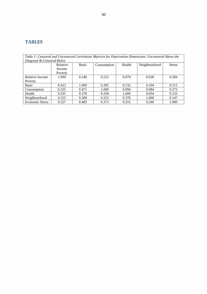
deprivation dimensions of moving from an uncensored to a censored approach. In Table 1 we

show the correlations between each of the dimensions (including income poverty), and

between them and economic stress. The uncensored outcomes are above the diagonal and the

censored below. Focusing first on the former we can see that the highest correlation of 0.395

is between basic and consumption deprivation. Of the remaining correlations, only those

relating to the basic and consumption deprivation relationships with relative income poverty

exceed 0.2. The average correlation is .144 The magnitude of these correlations has inevitable

consequences in minimising the numbers counted as deprived if one applies an intersection

approach with uncensored variables. Focusing on the correlations with economic stress, the

figure for basic deprivation is relatively high at 0.515 but the average correlation across all

dimensions is 291.

11

Turning to the censored data, we find a much more even pattern of correlation between

dimensions, reflected in an average correlation of 332 which is over double that in the

uncensored cases. The correlations with economic stress are also more uniform with the ratio

of the highest to the lowest correlation being 2.0 compared to 3.9 in the uncensored case. It is

clear that, conditional on being above the multidimensional poverty threshold, the association

between different forms of poverty/deprivation is considerably stronger. This in turn means

that the number of individuals fulfilling particular intersection conditions will be significantly

increased. In addition, as shown by the relationship to economic stress, the consequences of

exposure to forms of deprivation differ for those above versus below the multidimensional

poverty threshold.

Table 1 HERE

Multidimensional Poverty Levels by Country

In Table 2 we show the breakdown by country for the relative income poverty measure, M0

the adjusted head count ratio, H the headcount and I the mean intensity. To facilitate

interpretation we have ordered counties by their gross disposable income per capita (GNDH).

In column (i) we see the familiar pattern in relation to the relative income poverty measure

with very modest variation across countries. Somewhat higher levels are observed in the

counties with the lowest income levels. On the other hand, rates in former communist

counties such as the Czech Republic, Slovakia and Slovenia are considerably lower than in a

range of counties with higher income levels. The H headcount figures in column (ii),

indicates the number above the threshold, as a consequence of being above the cut off point

on at least two dimensions, reaches. In contrast to relative income poverty, we observe very

sharp variation across countries, which is broadly in line with average income levels. The

12

headcount figure ranges from a low of 0.083 in Norway to a high of 0.592 in Romania. There

is a clear tendency for the Scandinavian social democratic countries and the Netherlands

(often allocated to the same welfare ‘regime’) to report rates that are lower than might have

been expected purely on the basis of their average income levels. By contrast, Greece and

Hungary in particular exhibit rates somewhat higher than one might have expected from their

average incomes.

Column (iii) focuses on A the average intensity level among those who have been identified

as multi-dimensionally poor. Conditional on being identified as poor the intensity levels are

rather similar across counties. There clearly is a relationship between national income levels

and intensity with seven of the eleven counties with rates above 0.5 being among the eight

lowest income counties. However, outside these counties variation is extremely modest. The

headcount and intensity levels are clearly correlated but variation relating to former is a great

deal more pronounced.

In column (iv) we focus on M0 the adjusted head count ratio. This has a potential range of

values going from 0 to 1. Where no one in the population experiences any of the deprivations

it will take on a value of 0 and where every individual experiences deprivation on all items

the value will be 1. Our observed range of values goes from 0.030 for Iceland to 0.313 in

Romania. The intra correlation coefficient (ICC) is 0.108 indicating that just over 10% of the

total variances is accounted for by between country differences. As with the headcount index,

values generally increase as country income levels rise. Once again, values for countries in

the social democratic welfare regime are distinctively low. They range from 0.030 in Iceland

to 0.060 in the Netherlands and Norway. Countries that show slightly higher values than

might be expected on the basis of their income levels are Germany, the UK, Greece and most

particularly Hungary. For each of the three lowest income counties the adjusted head count

ratio exceeds 0.205. In other words, the multi-dimensionally poor experience an aggregate

13

level of deprivation that reaches over 25% of that which would be observed if

multidimensional poverty was universal and all poor individuals were deprived on all items.

Clearly the M0 measure is a great deal more successful in capturing cross-country variation

than the relative income poverty indicator. While the sharpest differential in the latter case is

2.3 in the former it reaches 10.4. In subsequent analysis we will provide a more systematic

analysis of such cross-country variation using multi-level models.

The figures for M0 can be contrasted with those for those for the union and intersection

counts for the five dimensions involved in our analysis as set out in columns (v) and (vi). For

the former, where all individuals experiencing deprivation on any of the dimensions is

counted the levels range from a lows of 0.301 in Iceland and 0..381 in Luxembourg to highs

of 0.808 and 0.821 in Bulgaria and Romania respectively. The figures in relation to the

intersection of the dimensions, involving deprivation on all five dimensions, provide a sharp

contrast. Here the counts range from close to zero in a large number of countries to 0.012 in

Bulgaria and 0.016 in Latvia.. The fact that the income poverty variable is defined in relative

terms contributes to the extreme nature of these results. However, they are generally

consistent with earlier research focusing on multiple deprivation in the European Union

Tsakloglou and Papadopouous (32) Whelan et al 2002 (34), Whelan and Maître (35). The

adjusted head count ratio clearly provides a middle ground between the union approach and

the intersection approaches.

TABLE 2 HERE

14

Decomposition of Multidimensional Poverty by Dimension

One of the advantages of the M0 measure is that it is decomposable in terms of sub-groups. A

related property is that sub-group consistency, which requires overall poverty to fall if

poverty decreases in one sub-group. Both properties are satisfied by the traditional FGT

measures and also by the A-F methodology. M0 is also decomposable in terms of dimensions.

In this case M0 is equal to the average of the censored head count ratio for the individual

dimensions and the percentage contribution of a given dimension to overall poverty is its

weighted censored head count ratio divided by the overall adjusted head count ratio..

In Table 3 we show this decomposition broken down by country for the dimensions in our

analysis. It is clear that there is substantial variation across countries in the relative

importance of dimensions. In the more affluent countries basic and consumption deprivation

generally play a less prominent role than other dimensions. In only four of the fifteen most

affluent countries does the figure for basic deprivation rise above .20 and in only five cases

does it do so for consumption. In no case is this value exceeded for both dimensions. The

combined basic and consumption deprivation rates range from 0.268 in the Iceland to 0.421

in German. In only two counties does it exceed .40. In the case of neighbourhood

environment the observed rate exceeds .20 only for the Netherlands the UK and Italy. Thus

for these countries the largest contributors to the AHR rate are the ARP and Health

dimensions. For the combined ARP and health dimensions the rate varies from .441in the

Netherlands to .539 in Norway.

The pattern for the six least affluent counties provides a sharp contrast. The lowest value of

the basic deprivation rate of .242 is observed for Hungary and the highest values of .329 and

.347 for respectively Romania and Bulgaria. For consumption deprivation the rates range

from .220 in Hungary to .309 in Romania. The combined basic and consumption deprivation

rate goes from .483 in Poland to .638 in Romania. For all of these counties the contribution of

15

neighbourhood environment is particularly modest and for the three least affluenct counties

the same is true of ARO and health deprivation

For the remaining counties variation across dimensions is somewhat more variable. As might

be expected the ARP measure makes a modest contribution in Slovakia and the Czech

Republic. In addition, Portugal and Estonia exhibit distinctively low rates of neighbourhood

deprivation.

TABLE 3 HERE

Socio-economic Variation in Risk Levels for Multidimensional Poverty

At this point we shift our attention from composition to risk levels and explore the extent to

which the impact of social class and age group on likelihood of multidimensional poverty

vary across counties. In Table 4 we break down M0 by an aggregated 7-category version of

the European Socio-economic Classification (ESeC) schema for the household reference

person (HRP) for each of the counties in our analysis.3 The class category for which the

sharpest degree of variation is observed is farmers, where the range runs from 0.020 in

Norway to 0.417 in Romania. Values are generally extremely low in the Scandinavian

countries. The ratio rises to between 0.050 to 0.126 for the remaining affluent Northern

European countries and the Czech Republic and Slovakia and Estonia. Values rise to between

0.159 0.169 for Cyprus, Greece and Portugal. Finally the remaining Eastern European

countries display considerable variation. Hungary, Poland and Lithuania exhibit values close

3 Malta has been excluded from this analysis and the analysis reported in Table 6 because of data problems

16

to the southern European countries. In contrast for the there least prosperous countries the

values rnage from .262 in Latvia to .434 in Romania.

For the remaining categories we observe a similar pattern of class differentiation across

countries. Generally the lowest values for M0 are observed for the higher professional and

managerial group. We also observe a consistent increase in rates moving from the more

affluent to the less affluent countries. The rate ranges from 0.005 in Sweden to 0.013 in

Romania. The next lowest level is observed for the lower professional and managerial class

where the rates go from 0 .011in Norway to 0.177 in Bulgaria. The corresponding range for

the lower white collar group is from 0.016 in Norway to 0.246 in Bulgaria. For the self-

employed group the corresponding figures are 0.032 in Norway to 0.328 in Romania. For the

higher working class group, the observed range goes from 0.033 in Iceland to figures ranging

from .337, .356 and .371 respectively for Latvia, Romania and Bulgaria. Finally, the highest

adjusted poverty ratio is generally associated with the routine working class group and those

classified as having never worked. The range runs from between 0.038 and 0.074 respectively

in Iceland and Norway and Sweden to in excess of .33 in Hungary, Latvia, Romania and

Bulgaria.

TABLE 4 HERE

The adjusted head count ratio clearly fulfills key requirements of a valid poverty measure in

that it varies systematically by social class group within countries, and across counties in

relation to national average income levels. The combined effect is reflected in the fact the full

range of variation for the M0 measure runs from 0.007 for the higher professional managerial

17

class in Luxembourg to 0.371 for the routine working class & never worked group in

Bulgaria – a disparity ratio of 53:1. Social class differences are substantial in every country.

We will address this issue more systematically in our subsequent analysis. The cumulative

effects of social class and country produces a situation whereby the most favoured social

classes in the least affluent countries exhibit lower poverty rates than the least favoured in the

more affluent countries. Thus in Norway and Denmark the value of M0 is respectively 0.074

and 0.086 while for the routine working class and never worked group while in Latvia and

Bulgaria the values for the professional and managerial class are respectively 0.123 and 0.135

At this point we shift our focus of attention to another potentially important socio-economic

variation in multidimensional poverty namely life-course. In Table 5 we show the breakdown

of M0 by the age group of the HRP. Variation across the life course is modest among the

more affluent countries. However, there is a tendency for the AHR level to be highest for tose

aged less than 30. For the eight of the ten countries with the highest average incomes per

capita the disparity ratio summarizing the ratio of M0 for the 65+ group to that for the <30

group does not exceed one. On the other hand for all thirteen lowest income countries the

highest level of AHR is observed for the group aged 65 or over.. In the more affluent counties

the lesser importance of basic and consumption seems to mute age differences. In other

words, where health deprivation comes in combination with basic deprivation it produces a

clear pattern of age differentiation, On the other hand, where it is to a significant extent

detached from such deprivation then that is not the case. This may be because the impact of

socio-economic deprivation on health is more clearly seen in older age groups.

TABLE 5 HERE

18

Multilevel Analysis of Multidimensional Poverty

Our analysis up to this point has been conducted at the level of the individual in order to

allow comparison with conventional poverty rates which are calculated at this level.

However, at this point since we wish to conduct a formal analysis of the distribution of

variance in relation to the adjusted head count ratio and since the construction of the

component measures ensures that all member of a household are assigned identical values on

each the dimensions included in our analysis,

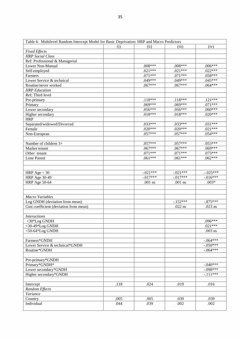
In Table 6 we present a set of hierarchical multilevel regressions with the adjusted head count

ratio as dependent variable. These are appropriate to a population with a hierarchical structure

where individual observations within higher level clusters, such as countries, are not

independent. Taking into account such clustering allows one to avoid “the fallacy of the

wrong level” involved in analysing data at one level and drawing conclusions at another and,

in particular, ensures that we do not fall prey to the ecological fallacy (Hox, 20).

Column (i) of Table 6 shows the results for the empty model with no independent variables.

The intra-class correlation coefficient (ICC) capturing clustering between counties is 0.108.

The ICC captures the between cluster variance as a proportion of the total variance. It can

also be interpreted as the expected correlation between two randomly drawn units from the

same cluster. (Snijders and Bosker,29). In column (ii) we enter a set of variables relating to

household and HRP characteristics. These comprise HRP social class, education, marital and

parental status, age group and housing tenure. The pattern of results is very much as we

would have expected with M0 being higher for the most disadvantaged educational, class and

labour force status, marital and parental status and tenure groups. The inclusion of this set of

variables reduces the deviance measured as -2 log likelihood ratio which is distributed as Chi

squared by 22,543 for 19 degrees of freedom. Taking into account compositional differences

19

in relation to such socio-economic attributes reduces the country variance by 1.9%, the

individual variance by 11.7% and the total variance by 10.6%.

TABLE 6 HERE

In equation (iii) we explore the impact of adding potentially important macroeconomic

influences on multidimensional poverty. In particular, we focus on the log of gross income

per capita (GNDH) and the Gini summary measure of income inequality, with both these

variables calculated as deviations from the mean to make later interaction analysis easier to

interpret. The values of the Gini variable have also been multiplied by 10 to eases

interpretation. The addition of these variables produces a modest reduction in the deviance of

20. The Gini variable is not statistically significant but GNDH with a coefficient of -/152 is

highly significant. This model reduces the country variance of the null model by 67.9% but

has no further effect on the household variance.

In equation (v) we provided a systematic exploration of the manner in which socio-economic

factors interact with GNDH. The coefficients for the socio-demographic variables involved in

the interactions are their values at zero deviation from the mean of the log of GNDH. Looked

at another way the coefficient for the log of GDH is the value where the set of socio-

demographic variables take on the reference category values. The interaction terms show a

consistent pattern of negative coefficients whereby socio-economic disadvantage has a more

pronounced effect at lower levels of GNDH. Similarly being in an older age group has a

sharper effect in less affluent counties. Again, taking an alternative perspective, we can

conclude that level of affluences is of greater consequence in explaining variations in

20

multidimensional poverty among disadvantaged socio-economic groups than for their more

favoured counterparts. For example the coefficient of 0.121 for pre-primary education

indicates the effect at the mean of log GNDH. The significant negative interaction of -0.044

indicates that the effect of such education relative to third level education declines as the

mean level of gross national income per capita increases and is accentuated at lower levels of

affluences. Similarly the significant coefficient of -0.025 for the <30 age group shows that at

the mean level of log GNDH this group is significantly less likely to be multi-dimensionally

poor than the 65+ group. However, the positive interaction coefficient of 0.096 indicates that

that this negative effect declines as the national income level increases and is correspondingly

magnified as it decreases.

Taking into account the manner in which household and HRP socio-economic characteristics

interact with national income reduces the deviance figure for equation (iii) by 2,604 for 10

degrees of freedom. Overall the model reduces the between country variance of the empty

model by 71%, the individual variance by 11.7% and the total variance by 18.2%. The multi-

level model analysis confirms that the adjusted head count ratio varies systematically across

socio-economic groups and countries but that a fuller understanding of these effects requires

that we take into account the manner in which micro and macro factors interact. The pattern

of interactions we observe is consistent with earlier analysis focusing solely on basic

deprivation (Whelan and Maître, 37). However, our ability to explain both within and

between country variance is somewhat less.

Multidimensional Poverty and Economic Stress

In this section, in order to further explore the validity of the measure of multidimensional

poverty we consider its relationship to subjective economic stress. In Table 7 equation (i) we

show the results for the empty model where economic stress is the dependent variable. The

21

intra-class correlation coefficient indicates that 14.6% of the variance in economic stress is

accounted for by between country differences. When H0 is entered in equation (ii) it has a

coefficient of 0.607. It reduces the between country variance by 0.499, the individual

variance by 0.198 and the total variance by 0.242. It reduces the log likelihood by 40,857 for

1 degree of freedom. Adding the log of GNDH in equation (iii) produces a significant

coefficient of -0.138 for that variable but has no impact on the coefficient for H0. The

addition of log GNDH reduces the likelihood by a modest 13.1. It also reduces the country

variance by 0.687 and the total variance by 0.270.4

The above analysis shows that, in addition to revealing expected patterns in relation to

country and social class, the adjusted head count ratio is a powerful predictor of economic

stress. This effect is not accounted for by its association with gross average national income

per capita. A comparison with findings by Whelan and Maître (38) focusing on basic

deprivation reveals that its impact is a good deal stronger than for H0. Despite the more

uniform impact of the deprivation dimensions on economic stress in the censored mode, there

is clearly some loss of explanatory power in subsuming different deprivation profiles under

the multidimensional poverty label. Extracting the full explanatory power of the original

continuous deprivation measure, required taking into account a significant interaction with

the log of GNDH with the effect of basic deprivation increasing significantly as average

income levels rose. The fact that this is not the case for H0 is likely to be a consequence of

these two effects cancelling each other out. Multidimensional poverty in less affluent

countries involves a higher proportion of basic deprivation. However, the impact of such

deprivation is greater in countries with higher income levels. The outcome is that H0 has a

uniform effect on economic stress across countries.5

4 Adding the Gini coefficient to the analysis produces no significant increase in explanatory power. 5 Adding the interaction terms reduces the log likelihood estimate by only 28.

22

TABLE 7 HERE

23

Conclusions

Multidimensional approaches to measuring poverty and social exclusion have as much

relevance in rich as in poorer countries and have received a good deal of attention in each,

with a substantial range of methodological approaches being advanced and applied. This

paper has applied to European countries the multidimensional poverty measurement approach

recently developed by Alkire and Foster (1,2,3,4), characterized by a range of desirable

axiomatic properties but mostly discussed so far in a development context. In doing so it has

exploited the potential of newly-available harmonized and more comprehensive microdata on

different aspects of deprivation for the European Union. Such an analysis requires measures

of a range of dimensions exhibiting reasonably satisfactory levels of reliability, with modest

variability in those levels across counties; the dimensions we have employed in our analysis

have been shown to fulfil these conditions to a much greater extent than was possible with

earlier waves of EU-SILC.

Our findings first demonstrate once again that what have been described as union versus

intersection approaches produce sharply contrasting results. The union approach leads to

rather trivial levels being defined as experiencing multidimensional poverty, certainly in the

better-off of the countries covered, while the intersection approach captures a very substantial

proportion of the population in every country and the vast majority of the population in the

least affluent counties . Application of the Alkire and Foster (1,2,3,4) approach in effect

provides a middle ground characterised by a set of desirable axiomatic properties. Central to

this approach is a censoring of data that counts deprivations only for those above the relevant

threshold: the strength of the correlations between the deprivation dimensions is then

substantially greater and the patterning of deprivation substantially more structured than for

24

their counterparts below the threshold, as one would want in a valid indicator of

multidimensional poverty and social exclusion.

In contrast to the conventional relative income poverty approach, the adjusted head count

ratio approach identifies a non-trivial minority as poor in each of the countries covered. The

size of this group varies in a fairly predictable manner with the country’s level of average

income per capita. The main source of such variation derives from corresponding variation in

the multidimensional head count: while the intensity level is also related to national income,

that variation is relatively modest, with those above the multidimensional threshold in every

case experiencing a high level of intensity.

A decomposition of multidimensional poverty by dimension also reveals systematic variation

across counties associated with national average income levels. In the less affluent counties

basic and consumption deprivation play a more prominent role while in their more affluent

counterparts relative income poverty and health are the key factors.

The overall level of multidimensional poverty varies significantly by national income level.

In contrast, income inequality as captured by the Gini coefficient has no such impact. It also

varies systematically by socio-economic group. In order to understand the distribution of

multidimensional poverty it is necessary to take into account the manner in which the latter

effects vary by national level of income. The impact of key factors such as social class,

education, and age are significantly stronger in low income countries. Thus both the nature of

multidimensional poverty and the extent to which it is socially stratified varies by national

level of income.

The adjusted head count ratio measure was found to be strongly related to levels of self-

reported economic stress, with an additional influence of national average income levels. The

ability to account for both within- and between-country variance in multidimensional poverty

25

is more restricted than it would be for a specific dimension such as the one we have termed

basic deprivation.

The advantages and disadvantages of a multidimensional perspective depend on the aims of

the analysis, the particular approach adopted and the manner in which it is implemented.

Furthermore, as Nolan and Whelan (25) emphasise, the identification of those exposed to

multidimensional poverty is primarily intended to help in understanding and addressing the

causes of poverty; the framework employed and groups identified can clarify or obscure

those causal mechanisms. This is a matter of immediate policy relevance, notably in the

European Union where a union approach combining three indicators (relative income

poverty, material deprivation and household joblessness) has been adopted to identify those

‘at risk of poverty and social exclusion’ in setting and monitoring a poverty reduction target

for 2020 (see Nolan and Whelan (26). In this context the EU Commission (11) argues that the

computation of a single indicator is an effective way of communicating in a political

environment, and a necessary tool in order to monitor 27 different national situations.

However, the ad hoc manner in which the EU poverty target has been framed serves to

highlight the advantages of a more structured approach such as the one proposed by Alkire

and Foster (1,2,3,4) and investigated here, within which the implications of crucial choices in

relation to dimensions, thresholds and weighting can be assessed in a consistent and

transparent way, and for which this paper is intended to serve as a base.

26

References

1. Alkire,S and Foster, J.: Counting and multidimensional poverty measurement, Oxford

Poverty & Human Development Initiative OPHI Working Paper 7 (2007)

2. Alkire,S and Foster, J.: Understandings and misunderstandings of multidimensional

poverty measurement, Journal of Economic Inequality, 9, 289-314 (20i1a).

3. Alkire, S and Foster, J. : Counting and Multidimensional Poverty’, Journal of Public

Economics, 95: 476-487 (2011b)

4. Alkire, A and Santos, M.E.: Acute multidimensional poverty: A new index for

developing countries, Human Development Research Paper (2010).

5. Alkire and Seth: Decomposing India’s MPI by state and caste: Examples and

comparisons, OPHI Research in Progress (2011)

6. Atkinson. A.: Multidimensional deprivation; contrasting social welfare and counting

approaches’, Journal of Economic Inequality, 1, 51-65 (2003)

7. Bourgignon, F. and Chakravarty, S.: ‘The Measurement of Multidimensional

Poverty’, Journal of Economic Inequality, 1, 25-49 (2003).

8. Cappellari, L. and Jenkins, S.P.: Summarising Multiple Deprivation Indicators in J.

Micklewright and S.P. Jenkins, eds., Poverty and Inequality: New Directions. Oxford:

Oxford University Press (2007).

9. Carle, A. C., Bauman, K. J. and Short, S.: Assessing the Measurement and Structure

of Material Hardship in the United States. Social Indicators Research, 92:35-5 (2009)

10. Dewilde, K.: The multidimensional measurement of poverty in Belgium and Britain:

A categorical approach. Social Indicators Research 68, 331-369 (2004)

11. European Commission: Employment and Social Developments in Europe 2011, DG

Employment, Social Affairs and Equal Opportunities (2011).

27

12. Eurostat: European social statistics: Income poverty and social exclusion (2nd

report), Office for Official Publications of the European Communities, Luxembourg

(2003)

13. Förster, M. F.: The European social space Revisited: Comparing poverty in the

enlarged European Union. Journal of Comparative Policy Analysis, 7, 1, 29-48 (2005)

14. Foster, J., Greer, J., Thorbecke, E.: A Class of Decomposable Poverty Measures,

Econometrica, 52, 3, 761-766 (1984).

15. Fusco, A, Guio, A-C and Marlier, E.: Characterising the income poor and the

materially deprived in European Countries, in A. B. Atkinson and E. Marlier (eds),

Income and Living Conditions in Europe. Luxembourg: Publications Office of th3

European Union (2010)

16. Grusky, David B., Weeden, Kim A.: Measuring poverty: The case for a sociological

approach. In: Kakawani, N., Silber, J. (Eds.), The Many Dimensions of Poverty.

Palgrave Macmillan, Basingstoke (2007)

17. Guio, A.-C.: Material deprivation in the EU, Statistics in Focus 21/2005, Eurostat,

Office for Official Publications of the European Communities, Luxembourg(2005)

18. Guio, A.-C.: What can be learned from deprivation indicators in Europe? Eurostat

methdologies and working paper, Eurostat, Luxembourg (2009)

19. Guio, A.-C. and Engsted-Maquet, I.: Non-income dimension in EU-SILC: Material

deprivation and poor housing, in Comparative EU statistics on income and living

conditions: Issues and challenges, proceedings of the EU-SILC conference, Helsinki,

November 6–8, 2006, Office for Official Publications of the European Communities,

Luxembourg (2007)

20. Hox, J.: Multilevel Analysis Techniques and Applications, Second Edition,

Routledge, New York and Hove.

28

21. Kakwani, N. & Silber, J. (Eds.): The Many Dimensions of Poverty. Basingstoke:

Palgrave Macmillan (2007).

22. .Layte, R., Maître, B., Nolan, B. and Whelan, C. T.: Explaining deprivation in the

European Union’, Acta Sociologica, 44 : 105–122 (2001)

23. Lustig, N.: ‘Multidimensional Indices of achievement and poverty: what do we gain

and what do we lose? An Introduction to the JOEI Forum on multidimensional

poverty’, Journal of Economic Inequality, 9, 227-234 (2011)

24. Moisio, Pasi.: A latent class application to the multidimensional measurement of

poverty. Quantity and Quality 38, 703-717 (2004)

25. Nolan, B. and Whelan, C.T. (2007). On the multidimensionality of poverty and social

exclusion. In Micklewright, J. and Jenkins, S. (Eds.), Poverty and Inequality: New

Directions. Oxford: Oxford University Press (2007)

26. Nolan, B. and Whelan, C.T.: Poverty and Deprivation in Europe, Oxford: Oxford

University Press (2011)

27. Pisati, M, Whelan, C. T., Lucchini, M. and Maître.: Mapping patterns of multiple

deprivation using self-organising maps: An application to EU-SILC data for Ireland.

Social Science Research, 39: 405-418 (2010).

28. Ravallion, M. (2011), ‘On Multidimensional Indices of Poverty; Journal of Economic

Inequality, 9: 235-248 (2011)

29. Snijders, T. and Bosker, R.: Multilevel Analysis. London: Sage Publications. (1999).

30. Thorbecke, E.: Multidimensional poverty: Conceptual and measurement issues. In N.

Kakawani & J. Silber (Eds.), The Many Dimensions of Poverty. Basingstoke: Palgrave

Macmillan (2007)

29

31. Tomlinson, M., Walker, A. and Williams, G.: Measuring moverty in Britain as a

multi-dimensional Concept, 1991 to 2003. Journal of Social Policy, 37, 597-620.

(2008)

32. Tsakloglou, P and Papadopoulos, F (2002). Aggregate levels and determining factors

od social exclusion in twelve European countries, Journal of European Social Policy,

12: 211-224

33. Whelan, C. T., Layte, R., Maître, B., & Nolan, B.: Income, deprivation and economic

strain: An analysis of the European Community Household Panel. European

Sociological Review, 17, 357–372 (2001).

34. Whelan, C. T., Layte, R., & Maître, B. Multiple deprivation and persistent poverty in

the European Union. Journal of European Social Policy, 12, 91–105 (2002)

35. Whelan, C. T. and Maître, B.: Vulnerability and multiple deprivation perspectives on

economic exclusion in Europe: A Latent Class Analysis. European Societies, 7,3,

423-450 (2005)

36. Whelan, C. T., Nolan B. and Maître, B.: Measuring material deprivation in the

enlarged EU, Working Paper No. 249, The Economic and Social Research Institute,

Dublin (2008).

37. Whelan, C. T. and Maître, B.: Understanding material deprivation in Europe: A

multilevel analysis, GINI Discussion Paper, Amsterdam Institute for Advanced

Labour Studies (2012a).

38. Whelan, C. T. and Maître, B.: Material deprivation, economic stress and reference

groups in Europe: An Analysis of EU-SILC 2009, GINI Discussion Paper,

Amsterdam Institute for Advanced Labour Studies (2012b)

30

TABLES

Table 1: Censored and Uncensored Correlation Matrices for Deprivation Dimensions: Uncensored Above the Diagonal & Censored Below Relative

Income Poverty

Basic Consumption Health Neighbourhood Stress

Relative Income Poverty

1.000 0.248 0.222 0.079 0.028 0.284

Basic 0.423 1.000 0.395 0.132 0.104 0.515 Consumption 0.325 0.471 1.000 0.094 0.084 0.373 Health 0.335 0.378 0.258 1.000 0.054 0.133 Neighbourhood 0.225 0.308 0.223 0.378 1.000 0.147 Economic Stress 0.327 0.483 0.373 0.255 0.240 1.000

31

Table 2: Multidimensional Poverty by Country EU-SILC 2009 (i)

Relative Income Poverty

(ii) MD

Headcount

(iii) MD Intensity

(iv) MD Adjusted

Headcount Ratio

(v) Union

(vi) Intersection

proportion proportion (2+)

proportion proportion

Luxembourg .149 .116 .469 .054 .381 .001 Norway .117 .083 .473 .060 .434 .001 Netherlands .111 .126 .476 .060 .434 .001 Austria .120 .165 .503 .083 .465 .004 Denmark .132 .115 .472 .054 .387 .002 Germany .155 .201 .530 .107 .489 .006 Belgium .146 .175 .523 .091 .423 .007 Finland .138 .139 .476 .066 .409 .002 UK .173 .212 .493 .105 .544 .002 France .129 .162 .500 .081 .438 .001 Spain 19.5 .213 .480 .102 .531 .002 Ireland .150 .192 .498 .096 .455 .002 Italy .184 .189 .452 .092 .512 .002 Iceland .150 .067 .484 .030 .310 .000 Cyprus .162 .166 .472 .078 .438 .001 Greece .197 .272 .499 .136 .606 .004 Slovenia .113 .166 .496 .082 .446 .004 Portugal .179 .330 .517 .171 .617 .005 Czech Republic

.086 .208 .491 .102 .569 .003

Malta 15.1 .186 .473 .088 .522 .001 Slovakia 11.0 .311 .507 .158 .668 .005 Estonia 19.7 .248 .494 .123 .551 .002 Hungary 12.4 .460 .521 .240 .770 .006 Poland 17.1 .310 .507 ..157 .637 .005 Lithuania 20.6 .320 .530 .170 .611 .008 Latvia 25.7 .456 .554 .253 .731 .016 Romania 22.4 .592 .529 ,313 .821 .006 Bulgaria 21.8 .535 .540 .289 .808 .012

32

Table 3: Decomposition of the Adjusted Head Count Social Exclusion Ratio by Dimension by Country EU-SILC 2009 ARP Basic Consumpti

on Health Neighbourhood Total

% % % % % % Luxembourg .276 .173 .146 .227 .178 1.0 Norway .281 .128 .220 .258 .112 1.0 Netherlands .199 .107 .133 .242 ,246 1.0 Austria .190 .205 .180 .265 .160 1.0 Denmark .236 .111 .226 .254 .172 1.0 Germany .215 .228 .193 .228 .136 1.0 Belgium .224 .186 .181 .228 .177 1,0 Finland .265 .092 .243 .269 .132 1.0 United Kingdom .212 .174 .136 .234 .240 1.0 France .206 .233 .179 .228 .154 1.0 Spain .238 .154 .216 .237 .156 1.0 Ireland .203 .154 .243 .217 .182 1.0 Italy .238 .208 .116 .230 .208

1.0

Iceland .243 .143 .125 .325 .166 1.0 Cyprus .257 .197 .153 .278 .116 1.0 Greece .223 .208 .214 .176 .179 1.0 Slovenia .173 .247 .156 .262 .162 1.0 Portugal ..161 .286 .211 .226 .116 1.0 Czech Republic .130 .164 .201 .282 .215 1.0 Malta .210 .286 .119 .183 .202 1.0 Slovakia .108 .184 .238 .243 .226 1.0 Estonia .230 .153 .250 .246 .126 1.0 Hungary .094 .289 .220 .205 .192 1.0 Poland .170 .242 .241 .226 .120 1.0 Lithuania .201 .321 .234 .220 .119 1.0 Latvia .179 .256 .225 .187 .154 1.0 Romania .134 .329 .309 .123 .106 1.0 Bulgaria .144 .347 .240 .120 .150 1.0

33

Table 4: Adjusted Head Count Ratio by Social Class and Country Higher

Professional &

Managerial

Lower Professional

& Managerial

Intermediate & Lower

Supv

Small Employer & Self-employ

Farmers Lower services & Clerical & technical

Routine & Never

Worked

Luxembourg .007 .019 .038 .073 .027 .100 .106 Norway .011 .011 .016 .032 .020 .052 .074 Netherlands .026 .053 .048 .056 .050 .069 .121 Austria .021 .040 .062 .087 .082 .109 .158 Denmark .025 ..030 .041 .042 .049 .050 .086 Germany .034 .040 .086 .098 .135 .137 .195 Belgium .020 .038 .064 .081 .063 .146 .196 Finland .022 .033 .062 .049 .083 .082 .104 UK .035 .054 .099 .101 .116 .137 .199 France .017 .032 .057 .068 .053 .104 .158 Spain .012 .027 .062 .102 .126 .133 .160 Ireland .032 .022 .071 .062 .040 .128 .180 Italy .025 .038 .053 .092 .098 .113 .136 Iceland .012 .019 .033 .048 .039 .033 .038 Cyprus .019 .026 .037 .109 .159 .090 .161 Greece .033 .042 .080 .142 .187 .185 .181 Slovenia .024 .041 .062 .062 .090 .098 .125 Portugal .040 .061 .089 .162 .248 .217 ,244 Czech Republic

.052 .066 .092 .050 .052 .119 .174

Malta Slovakia .078 .115 .140 .109 .116 .192 .224 Estonia .054 .088 .107 .056 .094 .135 .190 Hungary .101 .166 .214 .139 .199 .272 .339 Poland .045 .076 .123 .078 .185 .192 .224 Lithuania .075 .107 .123 .077 .141 .201 .229 Latvia .123 .146 .209 .177 .262 .296 .337 Romania .073 .155 .182 .328 .434 .319 .356 Bulgaria .135 .177 .246 .195 .309 .313 .371

34

Table 5: Mean Adjusted Head Count Social Exclusion Ratio by Age Group by Country EU-SILC 2009 <30 30-49 50-64 65+ Luxembourg .079 .054 .051 .052 Norway .068 .034 .025 .035 Netherlands .102 .055 .057 .057 Austria .113 .070 .090 .091 Denmark .097 .043 .040 .054 Germany .154 .088 .114 .119 Belgium .133 .081 .087 .109 Finland .078 .041 .061 .116 UK .111 .081 .083 .070 France .073 .070 .091 .098 Spain .085 .089 .102 .132 Ireland .116 .087 .107 .090 Italy .079 .073 .082 .119 Iceland .029 .024 .029 .039 Cyprus .080 .051 .071 .174 Greece .127 .110 ,125 .193 Slovenia .042 .060 .115 .143 Portugal .115 .136 .174 .219 Czech Republic .108 .090 .109 .119 Malta .082 .078 .083 .121 Slovakia .124 .140 .167 .230 Estonia .080 .088 .135 .233 Hungary .283 .222 .246 .258 Poland .118 .124 .176 .219 Lithuania .121 .142 .197 .259 Latvia .199 .221 .253 .370 Romania .253 .289 .323 ,345 Bulgaria .202 .236 .290 .385

35

Table 6: Multilevel Random Intercept Model for Basic Deprivation: HRP and Macro Predictors (i) (ii) (iii) (iv) Fixed Effects HRP Social Class Ref: Professional & Managerial Lower Non-Manual .008*** .008*** .006*** Self-employed .021*** .021*** .022*** Farmers .071*** .071*** .058*** Lower Service & technical .049*** .049*** .045*** Routine/never worked .067*** .067*** .064*** HRP Education Ref; Third level Pre-primary .118*** .118*** .121*** Primary .069*** .069*** .071*** Lower secondary .056*** .056*** .060*** Higher secondary .018*** .018*** .020*** HRP Separated/widowed/Divorced .033*** .033*** .031*** Female .020*** .020*** .021*** Non-European .057*** .057*** .054*** Number of children 3+ .057*** .057*** .053*** Market tenant .067*** .067*** .069*** Other tenant .071*** .071*** .073*** Lone Parent .061*** .061*** .062*** HRP Age < 30 -.021*** -.021*** .-.025*** HRP Age 30-49 -.017*** -.017*** -.016*** HRP Age 50-64 .001 ns .001 ns .003* Macro Variables Log GNDH (deviation from mean) -.152*** -.875*** Gini coefficient (deviation from mean) .022 ns .023 ns Interactions <30*Log GNDH .096*** <30-49*Log GNDH .021*** <50-64*Log GNDH .003 ns Farmers*GNDH -.064*** Lower Service & technical*GNDH -.050*** Routine*GNDH -.064*** Pre-primary*GNDH Primary*GNDH* -.040*** Lower secondary*GNDH -.098*** Higher secondary*GNDH -.111*** Intercept .118 .024 .019 .016 Random Effects Variance Country ;005 .005 .039 .039 Individual .044 .039

.002 .002

36

Intra Class Correlation Coefficient .108 .117 .042 .038 Reduction in country variance .019 .679 .710 Reduction in household variance .106 .106 .117 Reduction in total variance .092 .168 .182 Deviance -59,781 -82,315 -82,335 -84,939 N 199,354 199,354 199,354 199,354

Degrees of freedom 19 21 31 *p < .05 ** p < .01, *** p < .001

Table 7: Multilevel Regression of Adjusted Head Count Ratio and Log GNDH on Subjective Economic Stress (i) (ii) (iii)

H0 .646*** .648***

Log GNDH -.121***

Intercept .258 .184

Random Effects

Variance

Country

Individual

Intra Class Correlation Coefficient .125 .086 .061

Reduction in country variance .490 .650

Reduction in household variance .224 .224

Reduction in total variance .253 .268

Deviance 72,757 17,749 17,743

N 211,560 211,560 211,560

Degrees of freedom 1 2

*p < .05 ** p < .01, *** p < .001

37