uncongested mobility: the viability of a new jersey...

Uncongested Mobility: The Viability of a New Jersey Wide aTaxi

System

ORF467 Fall 2013

Professor Alain Kornhauser

January, 14 2014

Contents

1 Executive Summary 2

2 Motivation 6

3 Trip Synthesis 6

3.1 Trip Synthesis Process . . . . . . . . . . . . . . . . . . . . . . . . . . . . . . . . . . . . . . . . . . . . 7

3.1.1 Generation of Populace . . . . . . . . . . . . . . . . . . . . . . . . . . . . . . . . . . . . . . . 7

3.1.2 Assignment of Anchors . . . . . . . . . . . . . . . . . . . . . . . . . . . . . . . . . . . . . . . . 7

3.1.3 Assignment of Tours and Activity Patterns . . . . . . . . . . . . . . . . . . . . . . . . . . . . 7

3.1.4 Assignment of Temporal Attributes . . . . . . . . . . . . . . . . . . . . . . . . . . . . . . . . . 7

3.2 Multi-Modal Adjustments . . . . . . . . . . . . . . . . . . . . . . . . . . . . . . . . . . . . . . . . . . 7

3.2.1 Rail Transit . . . . . . . . . . . . . . . . . . . . . . . . . . . . . . . . . . . . . . . . . . . . . . 7

3.2.2 Spatial Modifications . . . . . . . . . . . . . . . . . . . . . . . . . . . . . . . . . . . . . . . . . 7

3.3 Naming our Population . . . . . . . . . . . . . . . . . . . . . . . . . . . . . . . . . . . . . . . . . . . 7

3.3.1 YellowPages.com Data . . . . . . . . . . . . . . . . . . . . . . . . . . . . . . . . . . . . . . . . 7

4 aTaxi System Design 7

4.1 The Grid System . . . . . . . . . . . . . . . . . . . . . . . . . . . . . . . . . . . . . . . . . . . . . . . 7

4.2 Trip Definitions . . . . . . . . . . . . . . . . . . . . . . . . . . . . . . . . . . . . . . . . . . . . . . . . 7

1

5 Statewide Analysis of New Jersey 7

5.1 Deep South Jersey: Salem, Cumberland, Cape May . . . . . . . . . . . . . . . . . . . . . . . . . . . . 8

5.2 South Jersey: Glouchester, Camden, Atlantic . . . . . . . . . . . . . . . . . . . . . . . . . . . . . . . 9

5.3 Jersey Shore: Burlington, Ocean . . . . . . . . . . . . . . . . . . . . . . . . . . . . . . . . . . . . . . 10

5.4 Route 18 Corridor: Monmouth, Middlesex . . . . . . . . . . . . . . . . . . . . . . . . . . . . . . . . . 11

5.5 U.S. Route 206 Corridor: Mercer, Somerset . . . . . . . . . . . . . . . . . . . . . . . . . . . . . . . . 12

5.6 Northwestern NJ: Sussex, Warren, Hunterdon . . . . . . . . . . . . . . . . . . . . . . . . . . . . . . . 13

5.7 North Jersey: Morris, Passaic, Bergen . . . . . . . . . . . . . . . . . . . . . . . . . . . . . . . . . . . 14

5.8 North East Jersey: Union, Essex, Hudson . . . . . . . . . . . . . . . . . . . . . . . . . . . . . . . . . 15

5.9 Out-of-State: New York City, Philadelphia, and International . . . . . . . . . . . . . . . . . . . . . . 16

5.10 Trip Type Distributions . . . . . . . . . . . . . . . . . . . . . . . . . . . . . . . . . . . . . . . . . . . 17

6 Moving Beyond New Jersey 18

7 Conclusions, Limitations, and Next Steps 18

2

1 Executive Summary

The objective of this project is to determine the viability of creating a fleet of autonomous taxi vehicles to effectively

serve the daily transportation demand in the state of New Jersey. The underlying goal is to leverage ride-sharing

of aTaxis to simultaneously easy congestion, increase safety, and reduce the environmental footprint of normal New

Jersey transporation behaviors. To achieve this aim, this project will simulate the 32 million daily trips taken by

New Jersey’s 8.89 million residents, characterizing each trip with an origin and destination and time of day. This will

be our test data set to assess the effect that introducing aTaxis would have on serving the personal transportation

demands of the United States’ most densely populated state.

Introduction: The Transporation Systems Planning and Analysis class (ORF467) in the Operations Research

and Financial Engineering Department at Princeton University has each year approached possible Personal Rapid

Transit (PRT) networks to serve travel demand in New Jersey with increasing complexity and improvements.

Through studying other PRT networks across the United States and the world, the inhibitive difficulties of traditional

PRT networks are evident. To serve travel demand en masse, the infrastructure costs required by PRT networks

are massive. There is also political and societal opposition that cites the unsightleness of independent guideways.

For a multitude of reasons, traditional PRT networks have never gained enough viability to accomplish a task such

as serving the travel demands of New Jersey.

However, with the advent of autonomous vehicle technology, there are technological advances that, we believe,

enable significant alternatives to traditional PRT networks. aTaxis are independently owned vehicles that drive

completely autonomously when given an origin and destination, and can respond to demand in real time. aTaxis

require no signficant improvements to guideways as they can operate on existing infrastructure. With such easy

integration into existing transportation networks, aTaxis avoid the debilitating realities of traditional PRT net-

works. With ridesharing a key motivation of the network proposed, there exists great opportunities to decrease

car ownership and thus decrease environmental impact. In addition, autonomous vehicles have an inherent safety

advantage over traditional vehicles. Autonomous vehicles are coming to market quickly and so we believe that an

aTaxi system is a PRT system of the future.

The first step of creating a transportation system for the state of New Jersey is to simulate a representative set

of trips taken daily in New Jersey. This means simulating trips not only in the state of New Jersey but in popular

nearby locations like New York City, Philadelphia, Bucks County (PA), and other out-of-state locations. Previous

ORF467 classes took great care to assemble data necessary. This year our three main sources of travel demand and

supply data were as follows:

3

• United States 2010 Census

• New Jersey State School System

• New Jersey State Employee and Patronage File

This data was used to create travel demand for each individual in the system. As a result, we could create a

specific trip tour for each individual that was built with both spatial and temporal characteristics. Having trips

organized by space and by time is crucial in our attempt to assess ridesharing potential within the system. This

year, we have continued to use the trip synthesizer developed as early as 2011 but enhanced year after year to

better match the data of New Jersey and provide a more realistic simulation with greater complexity. This year,

signficant efforts were made to introduce multi-modal trips, leveraging the existing NJTransit network of rail and

light rail within the state of New Jersey and main hubs of New York City and Philadelphia. In addition, this year

took great care to refine the Employee and Patronage file for businesses in the state of New Jersey.

This projects imagines a state wide aTaxi system where there are taxi stands within walking distance of every

origin and destination, so as to appropriately serve every trip. To meet the requirements that the stands be both

this accesible and this ubiquitous, we transformed the state of New Jersey into a grid system where each pixel is 0.5

miles by 0.5 miles. In this way, there is an aTaxi stand within a quarter mile, or 5 minute walk, to every origin and

destination. Trips are latitude and longitude to latitude and longitude. The grid system is a simple way to map

every trip from exact origin point to exact destination point to trips between pixels, or trips between aTaxi stands.

By overlaying the simulated transportation network on this grid system, we can assess how the aTaxi system would

serve the system by examining the activity and behavior of these aTaxi vehicles throughout a typical day.

With trips matching a typical day in the state of New Jersey generated, the first step was to filter by length.

Trips under 1.0 miles (or originating within one pixel of the destination) were considered to be walking or biking

trips. The remaining trips would be served by aTaxis, with the possibility of a multimodal split if taking a train

is a viable option. (See: Train Trip Multi-Modal Generation). The process at an aTaxi stand is not unlike that

of an elevator bank. You arrive to the elevator bank and wait to get into an elevator - sometimes you hold the

door for people to enter - and then you select your destination and it takes you there. People may get on and off

during your trip, at your floor or other floors on the way. So, passengers arrive to a station, and depending on given

parameters of the ridesharing model, the passenger enters the existing aTaxi that is going to the same destination,

or one nearby, or it gets in an entirely new aTaxi.

There are two main parameters considered for ridesharing models in this project. The first is Departure Delay

(DD). Departure Delay specifies the amount of time the aTaxi will wait at a station for passengers going to the

4

same destination as the original passenger. The most used DD times are 120 seconds and 300 seconds or 2 minutes

and 5 minutes. These were considered to be reasonable times passengers would be willing to wait to rideshare.

Using the elevator bank analogy, it is the time you are willing to hold the door open for passengers to get into

the elevator. The second parameter is Common Destination (CD). Common Destination refers to the number of

unique locations or pixels that an aTaxi can visit during a route. Again, using the elevator bank: CD is the number

of floors the elevator could stop at to allow people to exit. Both DD and CD are modulated in order to examine

different ridesharing models.

In our system, the following happens when a passenger arrives to a station:

1. Depending on the parameters of the ridesharing model imagined, the passenger enters the existing aTaxi if it

is going to the same or nearby destination as the passenger OR the passenger enters a new aTaxi

(a) If an existing aTaxi was entered, the aTaxi will continue to wait the specified departure delay remaining

from when the aTaxi first arrived at the station

(b) If a new aTaxi was entered, the aTaxi will wait the full departure delay time

2. The aTaxi departs the station after the departure delay to the destination(s)

Trip Visualizations In order to clearly emphasize the simplicty and elegance of our model the following graphs

will be used to explain how exact trips are transformed into aTaxi trips:

• Fundamental to our objective is the ability to easily aggregate trips at a very local level. Our solution was to

pixelize the state of New Jersey into small, walkable blocks whose centroid would be the location of an aTaxi

stand.

Figure 1: An Example of the 0.5mi x 0.5mi Pixel Structure

5

Figure 2: An Example of Mapping a Normal Trip to a Pixel to Pixel Trip

• We then mapped every trip to trips taken between aTaxi stands instead.

With this work done to all trips in our system, ridesharing potential, and other notable system characteristics

like trip volume and trip distribution, can be examined by geographical region (county) and for the state at large.

For ridesharing potential, the most important metric used to assess the viability of the system is Average Vehicle

Occupancy (AVO). The higher the number is above 1.0, the more ridesharing. AVO is calculated as:

AV O = PersonMiles/aTaxiMiles (1)

A related metric is Average Vehicle Occupancy at Departure. This is the number of passengers leaving a pixel

divided by the number of aTaxis leaving that same pixel.

HERE IS WHERE I WILL PUT ALL THE RESULTS COLLECTED, GATHERED FROM PPTS, RELATING

AVO TO COMBINATIONS OF CD AND DD, AS WELL AS P-¿P and P-¿SP. I WILL PUT TABLES AND

INITIAL CONCLUSIONS AND RESULTS.

Chapter Summaries Chapter 2 is a discussion of the motivation for an effective, large scale ridesharing system

and its implications. Chapter 3 details the exact trip synthesis process, and the validity of the simulated results

that make up the dataset for this project. Chapter 4 will discuss the aTaxi system we are proposing. Results and

analysis broken down by region in the state are contained in Chapter 5. In Chapter 6, we look beyond the state of

New Jersey and examine the feasibility of extending this project to the entire United States and present our initial

steps taken.

6

2 Motivation

3 Trip Synthesis

Trip Synthesis is one of the fundamental aspects of this project. In order to effectively assess the possibility and

efficacy of a state wide aTaxi system, the trips examined must match the trips taken on a typical day in NJ.

Furthmore, those persons taking the trips much match the real persons taking the trips in aggregate. To have

confidence in our final results means we must have confidence in our population synthesis and trip synthesis. That

means our population and trips must resonable mimic the aggregate features of the realistical, observed phenomena.

The method used in this project to generate out dataset was first proposed by the 2011 ORF467 class project

and Talal Mufti for is MSR thesis and enhanced by Jingkang Gao for his senior thesis.

7

3.1 Trip Synthesis Process

3.1.1 Generation of Populace

3.1.2 Assignment of Anchors

3.1.3 Assignment of Tours and Activity Patterns

3.1.4 Assignment of Temporal Attributes

3.2 Multi-Modal Adjustments

3.2.1 Rail Transit

3.2.2 Spatial Modifications

3.3 Naming our Population

3.3.1 YellowPages.com Data

4 aTaxi System Design

4.1 The Grid System

4.2 Trip Definitions

5 Statewide Analysis of New Jersey

Regional/County analysis - largest pixels, interesting results, special characteristics of county/region that make it

a good place for ridesharing.

At the top level, each summary is performed within a region. Each specific analysis is performed on each

individual oTrip files. There are, in some cases of larger counties, multiple oTrip files for a specific county. The

relevant analyses are done on the basis of number of trips in the file, total trip miles, median trip length, average

trip length, and a cumulative distribution of trip length. The files results are merged by county, and the county

results are in bold face in the tables. Furthermore, the trip type distribution for each county, or out-of-state region,

is presented. Trip types are, for example, Home to Other (H− > O), Work to School (W− > S), etc. Note: All

units are in miles.

8

5.1 Deep South Jersey: Salem, Cumberland, Cape May

Where the county codes for Salem, Cumberland, and Cape May are SAL, CUM, and CAP, respectively. Below is

the summary of results, followed by the graphs.

FileName

Numberof Trips

Trip Miles(millions)

Median TripLength (miles)

Average TripLength (miles)

Number ofTrips > 80m

SAL 199,319 2.693 11.927 13.243 340 (0.17%)CUM 527,573 9.708 19.448 18.401 1,296 (0.24%)CAP 203,896 4.402 24.668 21.590 2,164 (1.06%)

Table 1: Deep South Jersey oTrip Files

Figure 3: Cumulative Distribution of Trip Miles as a Function of Trip Length for Deep South Jersey

9

5.2 South Jersey: Glouchester, Camden, Atlantic

Where the county codes for Glouchester, Camden, and Atlantic are GLO, CAM, and ATL, respectively. Below is

the summary of results, followed by the graphs.

FileName

Numberof Trips





GLO−1 798,801 9.195 9.708 11.511 618 (0.08%)GLO−2 692,269 6.609 7.071 9.548 304 (0.04%)GLO 1,491,070 15.805 8.139 10.600 922 (0.06%)

CAM−1 829,654 8.354 7.433 10.069 468 (0.06%)CAM−2 655,710 6.748 6.964 10.292 291 (0.04%)CAM−3 712,969 7.830 7.762 10.981 204 (0.03%)CAM 2,198,333 22.932 7.433 10.432 963 (0.04%)ATL 796,530 19.462 24.274 27.434 889 (0.11%)

Table 2: South Jersey oTrip Files

Figure 4: Cumulative Distribution of Trip Miles as a Function of Trip Length for South Jersey

10

5.3 Jersey Shore: Burlington, Ocean

Where the county codes for Burlington and Ocean are BUR and OCE, respectively. Below is the summary of

results, followed by the graphs.

FileName

Numberof Trips





BUR−1 770,529 15.617 14.765 20.269 287 (0.04%)BUR−2 718,213 13.258 13.946 18.460 129 (0.02%)BUR 1,488,742 28.876 14.213 19.396 416 (0.03%)

OCE−1 683,240 16.069 22.699 23.519 1293 (0.19%)OCE−2 669,859 9.612 8.902 14.349 214 (0.03%)OCE 1,353,099 25.681 14.866 18.980 1,507 (0.11%)

Table 3: Jersey Shore oTrip Files

Figure 5: Cumulative Distribution of Trip Miles as a Function of Trip Length for the Jersey Shore

11

5.4 Route 18 Corridor: Monmouth, Middlesex

Where the county codes for Monmouth and Middlesex are MON and MID, respectively. Below is the summary of

results, followed by the graphs.

FileName

Numberof Trips





MON−1 733,496 11.655 11.629 15.890 256 (0.03%)MON−2 733,100 13.729 17.328 18.728 320 (0.04%)MON−3 729,093 12.568 14.431 17.238 502 (0.07%)MON 2,195,689 37.952 14.534 17.285 1,078 (0.05%)MID−1 861,634 10.737 11.511 12.462 112 (0.01%)MID−2 899,235 10.819 10.607 12.032 518 (0.06%)MID−3 747,156 9.041 9.552 12.100 204 (0.06%)MID 2,508,025 30.597 10.548 12.200 1,063 (0.04%)

Table 4: Route 18 Corridor oTrip Files

Figure 6: Cumulative Distribution of Trip Miles as a Function of Trip Length for the Route 18 Corridor

12

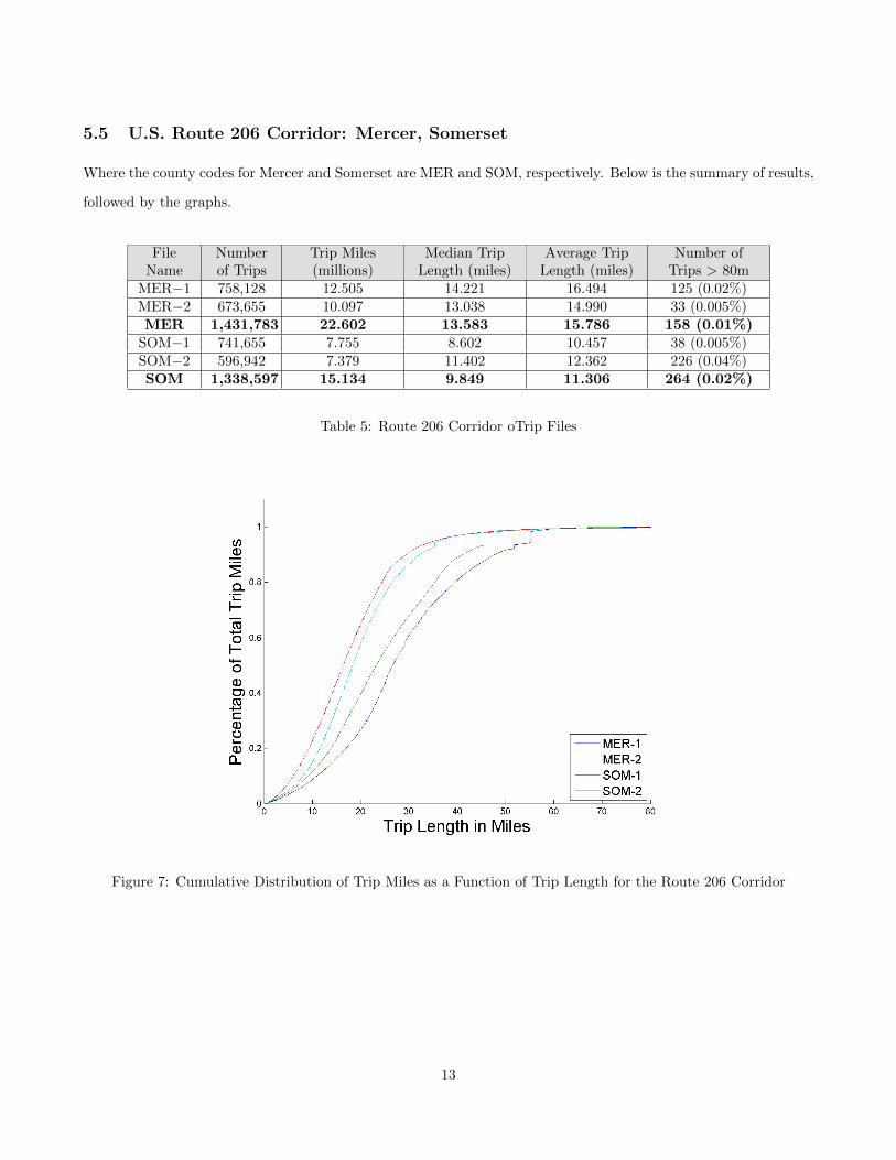
5.5 U.S. Route 206 Corridor: Mercer, Somerset

Where the county codes for Mercer and Somerset are MER and SOM, respectively. Below is the summary of results,

followed by the graphs.

FileName

Numberof Trips





MER−1 758,128 12.505 14.221 16.494 125 (0.02%)MER−2 673,655 10.097 13.038 14.990 33 (0.005%)MER 1,431,783 22.602 13.583 15.786 158 (0.01%)

SOM−1 741,655 7.755 8.602 10.457 38 (0.005%)SOM−2 596,942 7.379 11.402 12.362 226 (0.04%)SOM 1,338,597 15.134 9.849 11.306 264 (0.02%)

Table 5: Route 206 Corridor oTrip Files

Figure 7: Cumulative Distribution of Trip Miles as a Function of Trip Length for the Route 206 Corridor

13

5.6 Northwestern NJ: Sussex, Warren, Hunterdon

Where the county codes for Sussex, Warren, and Hunterdon are SUS, WAR, and HUN, respectively. Below is the

summary of results, followed by the graphs.

FileName

Numberof Trips





SUS 407570 6.528 14.705 16.016 409 (0.10%)WAR 301007 5.725 16.378 19.019 107 (0.04%)HUN 311202 5.222 16.007 16.781 69 (0.02%)

Table 6: Northwestern New Jersey oTrip Files

Figure 8: Cumulative Distribution of Trip Miles as a Function of Trip Length for Northwestern New Jersey

14

5.7 North Jersey: Morris, Passaic, Bergen

Where the county codes for Morris, Passaic, and Bergen are MOR, PAS, and BER, respectively. Below is the

summary of results, followed by the graphs.

FileName

Numberof Trips





MOR−1 728,416 9.758 11.413 13.397 542 (0.07%)MOR−2 772,588 11.397 13.647 14.752 580 (0.08%)MOR−3 631,504 8.227 10.630 13.027 451 (0.07%)MOR 2,132,508 29.383 12.042 13.779 1,573 (0.07%)PAS−1 629,753 4.893 6.042 7.770 513 (0.08%)PAS−2 667,237 6.522 8.201 9.774 727 (0.11%)PAS 1,296,990 11.415 7.106 8.801 1,240 (0.10%)

BER−1 955,955 6.292 5.657 6.582 1666 (0.17%)BER−2 758,359 6.976 8.732 9.198 1654 (0.22%)BER−3 797,402 10.162 13.238 12.744 1880 (0.24%)BER 2,511,716 23.429 7.566 9.328 5,200 (0.21%)

Table 7: North Jersey oTrip Files

Figure 9: Cumulative Distribution of Trip Miles as a Function of Trip Length for North Jersey

15

5.8 North East Jersey: Union, Essex, Hudson

Where the county codes for Union, Essex, and Hudson are UNI, ESS, and HUD, respectively. Below

is the summary of results, followed by the graphs.

FileName

Numberof Trips





UNI−1 794,736 6.485 6.519 8.160 271 (0.03%)UNI−2 959,633 8.443 7.159 8.799 429 (0.04%)UNI−3 959,633 8.246 6.500 8.417 440 (0.04%)UNI 2,734,238 23.175 6.727 8.476 1,140 (0.04%)

ESS−1 741,888 5.746 5.408 7.744 451 (0.06%)ESS−2 905,244 6.919 5.701 7.644 735 (0.08%)ESS−3 811,435 6.431 6.727 7.926 816 (0.10%)ESS−4 833,089 6.919 7.616 8.305 622 (0.07%)ESS−5 667,991 5.643 7.762 8.448 508 (0.08%)ESS−6 439,707 4.173 8.631 9.491 514 (0.12%)ESS 4,399,354 35.831 6.964 8.144 3,646 (0.08%)

HUD−1 770,003 6.322 6.519 8.209 583 (0.08%)HUD−2 1,007,975 6.633 4.610 6.581 808 (0.08%)HUD 1,777,978 12.955 5.590 7.286 1,391 (0.08%)

Table 8: North East Jersey oTrip Files

Figure 10: Cumulative Distribution of Trip Miles as a Function of Trip Length for North EastJersey

16

5.9 Out-of-State: New York City, Philadelphia, and International

Where the county codes for New York City, Philadelphia, Out-of-State, Rockland, Bucks, West, South, North are

NYC, PHL, INTL, ROC, BUC, WES, SOU, and NOR respectively. Below is the summary of results, followed by

the graphs.

FileName

Numberof Trips




Number of Trips >80m

NYC 451,867 7.814 13.583 17.292 0 (0.00%)PHL 98,761 1.714 12.042 17.354 487 (0.49%)INTL 2,995 0.074 21.006 24.670 0 (0.00%)ROC 46,739 1.137 20.670 24.334 624 (1.335%)BUC 156,328 5.074 30.069 32.462 358 (0.23%)WES 14,269 0.416 25.807 29.183 186 (1.30%)SOU 29,929 1.655 41.000 55.299 10,003 (33.42%)NOR 10,286 0.707 70.996 68.768 2026 (19.70%)

Table 9: Out-of-State oTrip Files

Figure 11: Cumulative Distribution of Trip Miles as a Function of Trip Length for Out-of-State

17

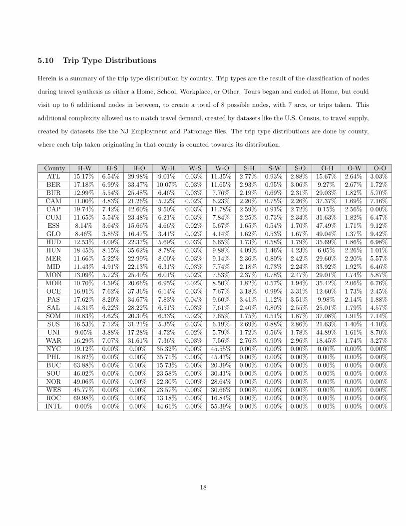
5.10 Trip Type Distributions

Herein is a summary of the trip type distribution by country. Trip types are the result of the classification of nodes

during travel synthesis as either a Home, School, Workplace, or Other. Tours began and ended at Home, but could

visit up to 6 additional nodes in between, to create a total of 8 possible nodes, with 7 arcs, or trips taken. This

additional complexity allowed us to match travel demand, created by datasets like the U.S. Census, to travel supply,

created by datasets like the NJ Employment and Patronage files. The trip type distributions are done by county,

where each trip taken originating in that county is counted towards its distribution.

County H-W H-S H-O W-H W-S W-O S-H S-W S-O O-H O-W O-OATL 15.17% 6.54% 29.98% 9.01% 0.03% 11.35% 2.77% 0.93% 2.88% 15.67% 2.64% 3.03%BER 17.18% 6.99% 33.47% 10.07% 0.03% 11.65% 2.93% 0.95% 3.06% 9.27% 2.67% 1.72%BUR 12.99% 5.54% 25.48% 6.46% 0.03% 7.76% 2.19% 0.69% 2.31% 29.03% 1.82% 5.70%CAM 11.00% 4.83% 21.26% 5.22% 0.02% 6.23% 2.20% 0.75% 2.26% 37.37% 1.69% 7.16%CAP 19.74% 7.42% 42.60% 9.50% 0.03% 11.78% 2.59% 0.91% 2.72% 0.15% 2.56% 0.00%CUM 11.65% 5.54% 23.48% 6.21% 0.03% 7.84% 2.25% 0.73% 2.34% 31.63% 1.82% 6.47%ESS 8.14% 3.64% 15.66% 4.66% 0.02% 5.67% 1.65% 0.54% 1.70% 47.49% 1.71% 9.12%GLO 8.46% 3.85% 16.47% 3.41% 0.02% 4.14% 1.62% 0.53% 1.67% 49.04% 1.37% 9.42%HUD 12.53% 4.09% 22.37% 5.69% 0.03% 6.65% 1.73% 0.58% 1.79% 35.69% 1.86% 6.98%HUN 18.45% 8.15% 35.62% 8.78% 0.03% 9.88% 4.09% 1.46% 4.23% 6.05% 2.26% 1.01%MER 11.66% 5.22% 22.99% 8.00% 0.03% 9.14% 2.36% 0.80% 2.42% 29.60% 2.20% 5.57%MID 11.43% 4.91% 22.13% 6.31% 0.03% 7.74% 2.18% 0.73% 2.24% 33.92% 1.92% 6.46%MON 13.09% 5.72% 25.40% 6.01% 0.02% 7.53% 2.37% 0.78% 2.47% 29.01% 1.74% 5.87%MOR 10.70% 4.59% 20.66% 6.95% 0.02% 8.50% 1.82% 0.57% 1.94% 35.42% 2.06% 6.76%OCE 16.91% 7.62% 37.36% 6.14% 0.03% 7.67% 3.18% 0.99% 3.31% 12.60% 1.73% 2.45%PAS 17.62% 8.20% 34.67% 7.83% 0.04% 9.60% 3.41% 1.12% 3.51% 9.98% 2.14% 1.88%SAL 14.31% 6.22% 28.22% 6.51% 0.03% 7.61% 2.40% 0.80% 2.55% 25.01% 1.79% 4.57%SOM 10.83% 4.62% 20.30% 6.33% 0.02% 7.65% 1.75% 0.51% 1.87% 37.08% 1.91% 7.14%SUS 16.53% 7.12% 31.21% 5.35% 0.03% 6.19% 2.69% 0.88% 2.86% 21.63% 1.40% 4.10%UNI 9.05% 3.88% 17.28% 4.72% 0.02% 5.79% 1.72% 0.56% 1.78% 44.89% 1.61% 8.70%WAR 16.29% 7.07% 31.61% 7.36% 0.03% 7.56% 2.76% 0.90% 2.96% 18.45% 1.74% 3.27%NYC 19.12% 0.00% 0.00% 35.32% 0.00% 45.55% 0.00% 0.00% 0.00% 0.00% 0.00% 0.00%PHL 18.82% 0.00% 0.00% 35.71% 0.00% 45.47% 0.00% 0.00% 0.00% 0.00% 0.00% 0.00%BUC 63.88% 0.00% 0.00% 15.73% 0.00% 20.39% 0.00% 0.00% 0.00% 0.00% 0.00% 0.00%SOU 46.02% 0.00% 0.00% 23.58% 0.00% 30.41% 0.00% 0.00% 0.00% 0.00% 0.00% 0.00%NOR 49.06% 0.00% 0.00% 22.30% 0.00% 28.64% 0.00% 0.00% 0.00% 0.00% 0.00% 0.00%WES 45.77% 0.00% 0.00% 23.57% 0.00% 30.66% 0.00% 0.00% 0.00% 0.00% 0.00% 0.00%ROC 69.98% 0.00% 0.00% 13.18% 0.00% 16.84% 0.00% 0.00% 0.00% 0.00% 0.00% 0.00%INTL 0.00% 0.00% 0.00% 44.61% 0.00% 55.39% 0.00% 0.00% 0.00% 0.00% 0.00% 0.00%

18

6 Moving Beyond New Jersey

7 Conclusions, Limitations, and Next Steps

19

uncongested mobility: the viability of a new jersey...

Documents