vii. the kohn-sham method

Electron Density Functional Theory

© Roi Baer

VII. The Kohn-Sham method

Kohn and Sham noticed that the HK theory is valid for both interacting and

non-interacting electrons. Now, they ask, what happens if for any system of

interacting electrons, with density there is a non-interacting system of the

same density? It is clear that if such two systems exist they are unique. The

non-interacting system has one advantage over the interacting system: we can

find its ground-state rather easily, since the many-body wavefunction is a

Slater wave function. So, the problem is: how to perform such a mapping.

A. Non-interacting electrons

If non-interacting electrons are tractable, let’s study their density functionals.

Given a density we assume it is non-interacting v-representable, i.e that

there exists a potential such that the ground-state of the non-

interacting Hamiltonian admits a ground-state having density

. The Hohenberg-Kohn functional for non-interacting electrons is reduced

to just the kinetic energy, i.e. we define:

(7.1.1)

As a private case of Eq. Error! Reference source not found. we have:

(7.1.2)

Thus, since our density is v-representable, is the minimizer of .

In other words, the ground-state wave function of non-interacting particles

associated with minimizes the kinetic energy! Let us see some

consequence this minimum principle.


© Roi Baer

A corollary, valid if the non-interacting system is non-degenerate, any

function for which equals must be the ground state

of the non-interacting system with density .

Let be the ground state wave function of the system of non interacting

electrons realizing the density . From the first equation in Eq.

Error! Reference source not found. one sees that realizes , thus

one can plug it into the right hand side of Eq. (7.1.2), with plugged into

:

(7.1.3)

Since now the right hand side is an expression of a scaled wave-function, one

can use Eq. Error! Reference source not found. and obtain:

(7.1.4)

And so . But we can also use this equation to scale back to

by dilating by , since: . Then, the same rule applies and we

get: , and so . We obtained two contradicting

equations which can agree only if both are reduced to equality. Thus:

(7.1.5)

This should be compared with the analogous result of Eq.

Error! Reference source not found. which is an inequality. The dilation effects

for non-interacting electrons is obviously much simpler. One important

corollary of (7.1.5) is that the non-interacting wave functions scale with the

density. We saw that gives the correct kinetic energy of for the system

with density , , and therefore, necessarily:

(7.1.6)


© Roi Baer

Exercise

1) We can define a functional called the Hartree energy, which is the

classical electrostatic energy associated with the charge distribution

:

(7.1.7)

Prove the following dilation relation:

(7.1.8)

2) Now define the exchange energy functional (see also Eq.

Error! Reference source not found. for a definition based on the

orbitals):

(7.1.9)

Use (7.1.6). Prove:

(7.1.10)

What is the relation between the potential for which is a non-

interacting ground state density and for which is a non-

interacting ground state? We can use the basic DFT equation to answer this.

From the basic definition of functional derivation:

(7.1.11)

The 3D delta-function has the density dilation structure:

, so:

(7.1.12)


© Roi Baer

Then using Eq.:

(7.1.13)

By dilating in the reverse direction we can easily see that:

(7.1.14)

We could have obtained this result directly from the Schrödinger equation.

Suppose is a many-body eigenfunction of Hamiltonian ,

i.e . Define a scaled wavefunction:

(7.1.15)

Then clearly:

(7.1.16)

And so with energy and potential given

by:

(7.1.17)

For a ground state of non-interacting the first equation means that

is the one-particle potential for the scaled determinant, and thus for

the scaled density (since the scaled determinant realizes the scaled density).

B. Orbitals for the non-interacting electrons

Consider the ground state wave function for the non-interacting electrons

. Suppose the non-interacting electrons reside in the potential (the


© Roi Baer

subscript is in honor of Slater) then . In most

cases this wave function is a normalized Slater wave function. We introduce

orthormal spin-orbitals , from which is built. These

orbitals are excited states of the potential well in which the non-interacting

electrons reside. Thus the orbitals must each obey the single-electron

Schrödinger equation:

(7.1.18)

The orbitals correspond to the lowest eigenvalues . The fact that

realizes the density is expressed as :

(7.1.19)

The non-interacting kinetic energy is then:

(7.1.20)

When one wants to find the functional derivative of with respect to

one can turn to basic equation, Eq. Error! Reference source not found. which

in case of non-interacting electrons becomes:

(7.1.21)

We will see that this equation is important for the method known as the

Kohn-Sham method.

Note that the discussion of dilation in the previous subsection can be carried

on to the orbitals. The only additional information to convey is that the


© Roi Baer

orbitals scale as the density and each of the orbital energies scale as the total

energy:

(7.1.22)

C. The correlation energy functional: definition

and some formal properties

The ground state energy of the an system of electrons in density can be

written in terms of the non-interacting (Slater wave function) wave function

:

(7.2.1)

This equation is actually a definition of a new density functional, the

correlation energy functional . If we suppose for the time being that

is known, this expression can be used to define a working procedure

for DFT known as the Kohn-Sham method. From our studies of the Hartree-

Fock theory, we know that the expectation value of within a determinant

can be written as:

(7.2.2)

Where is the Hartree energy:

(7.2.3)

And is given in terms of the orbitals from which is composed (Eq.

Error! Reference source not found.):

(7.2.4)

Based on this, we rewrite as:


© Roi Baer

(7.2.5)

This allows us to write Eq. (7.2.5) compactly as:

(7.2.6)

Clearly we have also the equivalent equation:

(7.2.7)

Physical intuition concerning molecules and solids tells us that is a

small quantity when compared to or . Thus, it is reasonable to look

for approximations to this quantity. Approximation to the correlation energy

functional is the most important issue in DFT. It is an open question, still

being worked upon.

We shall deal with approximations later. Meanwhile, let us ask what can be

safely said about the correlation functional. We prove here several important

inequalities. First, consider the difference , the correlation

kinetic energy.

Exercise

Show is a positive quantity. This is actually intuitively clear: the

interacting electrons must have much more complicated "paths" in the

interacting case because they want to avoid "bumping into" other electrons.

Anything with more swirls must have higher kinetic energy.

Solution

Using the variational theorem:

(7.2.8)


© Roi Baer

Where is the interacting ground-state wave function determined by .

Comparing the two sides we have:

(7.2.9)

Next, we can show that the exchange correlation energy is always negative.

This comes about from our experience with expectation values of

determinants:

(7.2.10)

Using Eq. (7.2.6) we find:

(7.2.11)

Furthermore is negative as can be seen from the fact that

is negative and is positive:

(7.2.12)

An additional property is the dilating relations. We have proved that

and , . Thus:

(7.2.13)

One way to proceed is to substitute with . The other is to substitute

with . We obtain from each possibility:

(7.2.14)

And, since is always positive and negative, we find that:

(7.2.15)

Obviously, the second relation is contained in the first (since ) and so

only the first relation is important; it can be used to derive complementary

inequalities. Indeed, applying them for we find:


© Roi Baer

(7.2.16)

This holds for any , so we stick in (7.2.16) instead of and using the fact

that to obtain:

(7.2.17)

In absolute values:

(7.2.18)

Intuitively, the larger the more correlation we have. We see that

compressing the density, say on the average by a factor 8 ( ) does not

necessarily raise the abs value of the correlation energy, certainly not by more

than a factor 2.

D. The Kohn Sham equations

i. The Kohn-Sham equation from a system of non-interacting problem

Let us now turn to the issue of determining , required for the mapping

between the interacting non-interacting systems. Let us start form the basic

equation Eq. Error! Reference source not found. which becomes, using Eq.

(7.2.6):

(7.3.1)

Where:

(7.3.2)

is the Hartree-Exchange potential. Notice that:

(7.3.3)

and:


© Roi Baer

(7.3.4)

Thus, from Eq. (7.1.21) and Eq. (7.3.1) (up to a constant):

(7.3.5)

This equation gives us the potential of the non-interacting system. Thus, we

have made a definite connection between the interacting and non-interacting

systems.

Now, an important observation allows us to set up a simple method for

obtaining the ground-state of an interacting system of electrons. We need to

find a density that obeys two conditions:

a) It is the density of the non-interacting electrons so it is the sum of square

orbitals (Eq. (7.1.19)) that obey the Schrödinger equations (7.1.18) with

potential .

b) The potential must be related to the interacting system by Eq. (7.3.5)

This leads to a simple SCF procedure, called "The Kohn-Sham method"

reminiscent of the Hartree-Fock algorithm:

1. Guess .

Build , from (Eq. (7.3.3) and (7.3.4)).

Obtain the orbitals from the lowest eigenvalues of Eq. (7.1.18).

Compute the density from Eq. (7.1.19)

Redo from step 2 using the new density until you converge – i.e. until the

density changes no more.

When the process convergence, we have the exact ground-state density .

It can be used to compute the ground-state energy by plugging it into the

energy functional of Eq. Error! Reference source not found.:

(7.3.6)


© Roi Baer

ii. Systems with partially occupied orbitals

Partially occupied orbitals arise in the realm of ensemble-DFT, i.e. when the

density searched for is not “non-interacting v-representable”. We still assume

the density is a sum of orbital densities as follows:

(7.3.7)

but unlike Eq. (7.1.19) we do not impose exactly orbitals. The orbitals are

almost completely unconstrained, except for the Fermionic condition, that

their norm must be not be great than 1:

(7.3.8)

but the total number of electrons is still :

(7.3.9)

And the kinetic energy is written similarly to Eq. (7.1.20):

(7.3.10)

We generalized Eqs. (7.1.19) and (7.1.20) any number of orbitals leading to the

following orbital Lagrangian:

(7.3.11)


© Roi Baer

and are Lagrange multipliers assuring orbital normality and

total number of particles. We minimize the Lagrangian with respect to the

orbitals and the occupation numbers (constraint to be non-negative and

not greater than 1). The constraint minimum procedure thus requires that:

(7.3.12)

The first equation leads to the KS equations:

(7.3.13)

For convenience, we order the indexing so that the series of orbital energies is

ascending: The orbitals are now eigenfunctions of a Hermitian

Hamiltonian, and so we can assume they are orthogonal:

(7.3.14)

We define as a short-hand notation (see Eq.

(7.3.5)). By multiplying Eq. (7.3.13) by integrating on and summing on

q we find:

(7.3.15)

The second condition for minimum of holds only in cases that the

minimum is attained with non-integer electron number, . The cases

or are the boundary of the constraints and the derivative need

not be zero there. From this second part of the equation, we have:

(7.3.16)

This shows that all incompletely occupied orbitals have the same orbital

energy equal to the chemical potential , the Lagrange multiplier imposing


© Roi Baer

the number of particle constraint of the Hohenberg-Kohn theory (Eq.

Error! Reference source not found.).

Typically, all orbitals with are fully occupied ( and those with

are fully unoccupied ( . The interacting electron energy is

obtained using Eqs. (7.3.6) and (7.3.15) as

(7.3.17)

We should note that the development here assumed non-interacting v-

representability. In cases where this is not valid other occupation rules may

apply.

iii. Is the ground state wave function of non-interacting particles always a

Slater wave function

The standard KS approach to the non-interacting kinetic energy is by defining

the functional as a minimum principle on the manifold of single

determinants:

(7.3.18)

Setting up a Lagrangian and searching for the constrained minimum yields

occupied orbitals. If the density is not v-representable one or more of the low

energy orbitals may have 0 occupation numbers.

Another way to define a non-interacting kinetic energy functional is by an

extended minimum search over more general wave functions:

(7.3.19)

Usually this search ends with being a single Slater wave function and for

these case and given are the same. Yet, this may not always be the case.


© Roi Baer

Let us assume that we are searching through all

where or are Slater wave functions. In general, the kinetic energy is

then:

(7.3.20)

Now, if and differ by only one orbital (say

for )

then is actually a Slater wave function: its orbitals are the ’s and

then a new orbital

is added. Next, if and

differ by two (or more) orbitals the cross term in (7.3.20) is zero and the

kinetic energy is simply the sum of orbitals kinetic energies with occupation

numbers given by and . The orbitals shared by the two

determinants will have unity occupation number (since )

while orbitals in the determinant but not in the B determinant will have

occupation number and those in the determinant but not in the A

determinant will have occupation number . The orbitals coming out

from the minimization will all solve a Schrödinger equation with the same

potential. The 4 odd orbitals (2 from each determinant) will all have the same

orbital energy equal to . When there are more than 2 Slater wavefunctions a

similar treatment will result and even more orbitals will be degenerate at the

chemical potential. Even if is v-representable this type of wave function can

arise.

A third way to define the kinetic energy is as an ensemble average. Instead of

a wave function, one uses a mixed density matrix . The

constants are positive and sum to 1. The density is the convex sum

of densities from each participating determinant. A similar

expression will arise for the kinetic energy. This approach is designed to solve


© Roi Baer

the problems of non-interacting v-representability emanating from convex

sums of degenerate wave functions (see section XXX).

iv. Janak’s Theorem

A very general theorem was noted by Janak 5, based on earlier work of Slater

and Wood6 concerning the meaning of orbital energies. Let us return to the

functional of Eq. (7.3.11) and assume now that the occupation numbers are

given and they are all non-negative and not larger than 1 and that they sum

up to the number of electrons. Thus, for a given set of occupation numbers we

can search for the orbitals that minimize the following functional:

(7.3.21)

The equations that the orbitals must obey are still derived from Eq. (7.3.12)

leading to the same equations as in (7.3.13), the KS equation. Now, let us ask:

what happens to the energy when we change the occupation number of one

of the orbitals by an infinitesimal amount When we do this the “total

number of electrons” changes by this amount as well. This is not a physical

change (since electrons cannot change by non-intereger amounts) but still

mathematically speaking the change can be studied. Since are the

constraints and the Lagrange multipliers in a minimization problem we can

use the general result of Eq. Error! Reference source not found. that the rate

at which the minimized function changes when the constraints change is

equal to the Lagrange multiplier:

(7.3.22)


© Roi Baer

This relation, giving some meaning to the orbital energies is called Janak’s

theorem. This theorem is quite general but relies on some analytical

assumptions of the energy functional. For example, when the occupation

number is 1 the change can only be by a negative amount and when it is zero

– only positive. For approximate functionals, that are analytical with respect

to any and this relation holds. Such is the case for the often used

local, semilocal and even most hybrid functionals, including Hartree-Fock

theorem.

In the conext of Hartree-Fock theory this result is a restatement of Koopmans’

theorem, by which is the unrelaxed ionization energy from orbital . The

orbital relaxation is a second order effect and thus negligible when occupation

numbers change infinitesimally.

E. “Virial Theorem” related identities in DFT

The following development is inspired by the virial theorem treatment. It

continues to consider dilation relations. Taking the derivative of with

respect to , we have

and since,

, we find

(7.4.1)

For a general density functional, , we have, using the chain rule for

derivatives, and Eq. (7.4.1)then:


© Roi Baer

From which a completely general virial-dilation relation holds for any

functional:

(7.4.2)

We will be especially interested in the case of . Thus the basic relation:

(7.4.3)

We further find that

(7.4.4)

Let us apply this for the Hartree energy. From Eq. (7.1.8) we find the following

relation, valid for any : so:

(7.4.5)

A similar relation, namely hold also for the exchange

energy (see Eq. (7.1.10)), and so:

(7.4.6)

Where is the exchange potential.

Now, what about the correlation energy? Let us consider the KS DFT

functional:

(7.4.7)

Suppose is the density minimizing minimizer of and now plug into

the latter the scaled density. This will give a dependent energy:

(7.4.8)


© Roi Baer

And clearly, the minimum is at so:

(7.4.9)

Now, let us evaluate using Eq. (7.1.5):

(7.4.10)

and plug in . We obtain:

(7.4.11)

or, using Eq. (7.4.3):

(7.4.12)

The second term in the parenthesis can be related to the interacting system.

Indeed we have, using Eqs. Error! Reference source not found.:

(7.4.13)

Taking the derivative with respect to , remembering that we

find, for :

(7.4.14)

(As a sidenote, you can see that substituting this relation in Eq. (7.4.1) gives

after trivial manipulation the virial theorem

). Continuing the above development, using Eqs. (7.4.11) and

(7.4.14) we finally find:


© Roi Baer

(7.4.15)

which can be written equivalently as:

(7.4.16)

or, using Eq. (7.4.3):

(7.4.17)

The Hartree and exchange energies give zero while the correlation energy

gives a negative quantity equal exactly to

This result shows that the correlation energy functional and the correlation

potential are enough for determining the correlation kinetic energy (and from

it, by ) the kinetic energy itself.

This latter result is related to the virial theorem of Slater, which shows that

one can derive the kinetic energy of the electrons from the Born-Oppneheimer

potential surface itself (Eq. Error! Reference source not found.). Since DFT

gives, in principle the Born-Oppenheimer potential surface, one can access the

kinetic energy (and the potential energy) from the DFT calculation.

F. Galilean invariance

A basic property of the electron-electron interaction is that if the coordinates

of all electrons are shifted by a constant :

(7.5.1)

the e-e interaction enegy does not change

(7.5.2)


© Roi Baer

This property is shows that the e-e interaction is translationally invariant. This

property is also called Galilean invariance. The same property holds when the

coordinates of each electron are rotated around some axis. This roatation can

be described by a 3×3 orthogonal matrix , where :

(7.5.3)

The lengths of vectors are preserved under a rotation:

(7.5.4)

Thus the e-e interaction enegy does not change

(7.5.5)

Thus the e-e energy is rotational invariant.

These relations indeed hold for the density functional since it is a

reflection of the e-e functional. Indeed, define the shifted density:

(7.5.6)

Then:

(7.5.7)

We now make a variable replacement: and obtain:


© Roi Baer

(7.5.8)

This condition, that is called Galilean invariance. It is easy to

show that functional is also rotational invariant.

The exchange energy is also Galilean invariant, since the translation of the

density will cause a translation of the density matrix:

(7.5.9)

It is easy based on this to show that

Finally, the same will hold for the kinetic energies , . All this shows

that we must demand this invariance of the correlation energy:

(7.5.10)

One consequence is the property of Galilean covariance of the potentials for

each of the above energy functionals. For example, for the correlation energy

we have the following result. Suppose we shift the density by a small

displacement:

Thus:

(7.5.11)

Since we demand Galilean invariance we find:

(7.5.12)

Since

and is arbitrary:


© Roi Baer

(7.5.13)

For finite systemswhere the density drops to zero at infinity we can move the

nabla sign to the potential:

(7.5.14)

is the force derived from the correlation potential. This shows that

the total correlation force is always zero. Another consequence from Galilean

invariance of the correlation energy is the Galilean covariance:

(7.5.15)

Similar conditions can be proved from rotational invariance. For example the

torque:

(7.5.16)

G. Holes and the adiabatic connection

i. The exchange and correlation holes

Let us now take a step back and return to wave function theory. We examine

the electron-electron interaction energy

(7.6.1)

Which we write using the following operator:

(7.6.2)

In the first term, we sum over the pairs of r-vectors of each of the

coordiantes (indices and ). In the second term we use the definition:


© Roi Baer

(7.6.3)

which is the pair density operator. Note the relation between the one and two

densties:

(7.6.4)

With . With this definition, we have:

(7.6.5)

The expectation value of is the "two electron density function":

(7.6.6)

With the two-electron density function, the interaction energy is:

(7.6.7)

This pair density function has the symmetry, positivity and normalization

properties given by:

(7.6.8)


© Roi Baer

The normalization allows interpretation of

as the probability density to

find an electron at and another electron at . One property that is intuitively

expected of is as the limit is approached electrons will

gradually uncorrelate and collapse to the density product .

Indeed, this is insight bears out in most cases:

(7.6.9)

but not always. For example, the ground state wavefunction of the Carbon

atom (we are neglecting to write spin indices for sake of

notational simplicity) in the large limit: for minimal energy reasons the

remaining electrons will lower their energy to a maximal extent thus, the

wave function should obey:

where

is the ground state wave function of the cation and

is

the root of the propability to find an electron far at . Note however that this

cation has a 3-fold degeneracy in its groundstate energy and thus for any

finite , no matter how large, the wave function is that

degenerate wave function distorts in a certain fashion in correlation with the

direction (for more details see Phys. Rev. A 49, 809 (1994) or J. Chem.

Phys. 105, 2798 (1996)).

We can also look at the conditional probability density to find an electron at

given that there is one at (this latter probability is ), given by

(7.6.10)

Obviously, if one integrates on one gets unity. We can thus view:


© Roi Baer

(7.6.11)

as a “conditional” density, the density at of electrons: all “other”

electrons except that one electron is known to be at . Indeed, upon

integration over , we get, irrespective of :

(7.6.12)

Furthermore, we have for :

(7.6.13)

This shows that the density far from the localized electron is unperturbed.

Now, let us subtract from this conditional density the total -electron density

and obtain the Fermi-Coulomb hole function:

(7.6.14)

Since we localized an electron at the rest of the electrons will “rearrange” so

as to be repelled from the stationary source. This will give us a “missing

density” or “hole density”, i.e. the charge density at expelled by an electron

at . We expect the total charge of the hole is . Indeed plugging Eq. (7.6.14)

into (7.6.12) we find:

(7.6.15)

Furthermore far from the hole center we have from Eqs. (7.6.13) and (7.6.14) :

(7.6.16)

This shows that the FC hole decays faster than the density far from the

system: for localized systems it is, in most cases, a highly localized overall

singly charged distribution.


© Roi Baer

Now, because

, the

Coulomb interaction energy can be written as:

(7.6.17)

And in terms of the FC hole:

(7.6.18)

Thus the part of the interaction energy beyond the Hartree energy is the sum

of all interaction energies

between an electron at

and its Fermi-Coulomb hole . We will shortly see that the correlation

energy adimits a similar analysis only with slightly modified quantities.

By using non-interacting electrons we can also pull out of the integral the

exchange energy and write:

(7.6.19)

This leaves a Coulomb hole which is overall neutral. It too is localized. We

discuss this in the section after next.

ii. The Fermi-Coulomb hole for harmonic electrons

Let us calculate these quantities for our 2-harmonic electrons in their ground

state triplet (so we have both exchange and correlation). The pair density and

density for the wave function in Error! Reference source not found. is:

(7.6.20)

The density can be obtained by integrating:


© Roi Baer

(7.6.21)

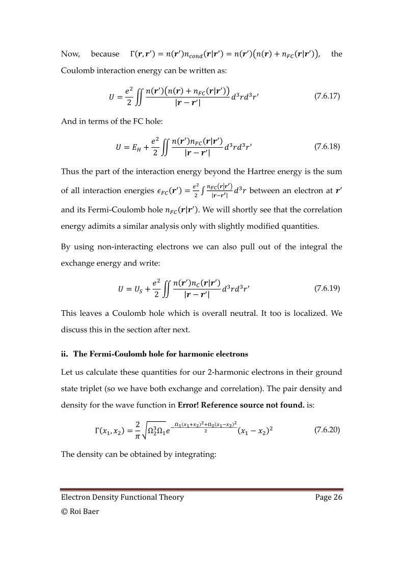
The density is plotted for several values of the correlation constant ,

. This calculation is for :

Figure ‎VII-1: The 1-particle density, for a system of two harmonic fermions placed in a

harmonic well in their triplet ground state for various interaction strengths. When

there is no interaction and the dip in is due to the “Pauli repulsion”. As interaction

grows the dip becomes deeper and broader.

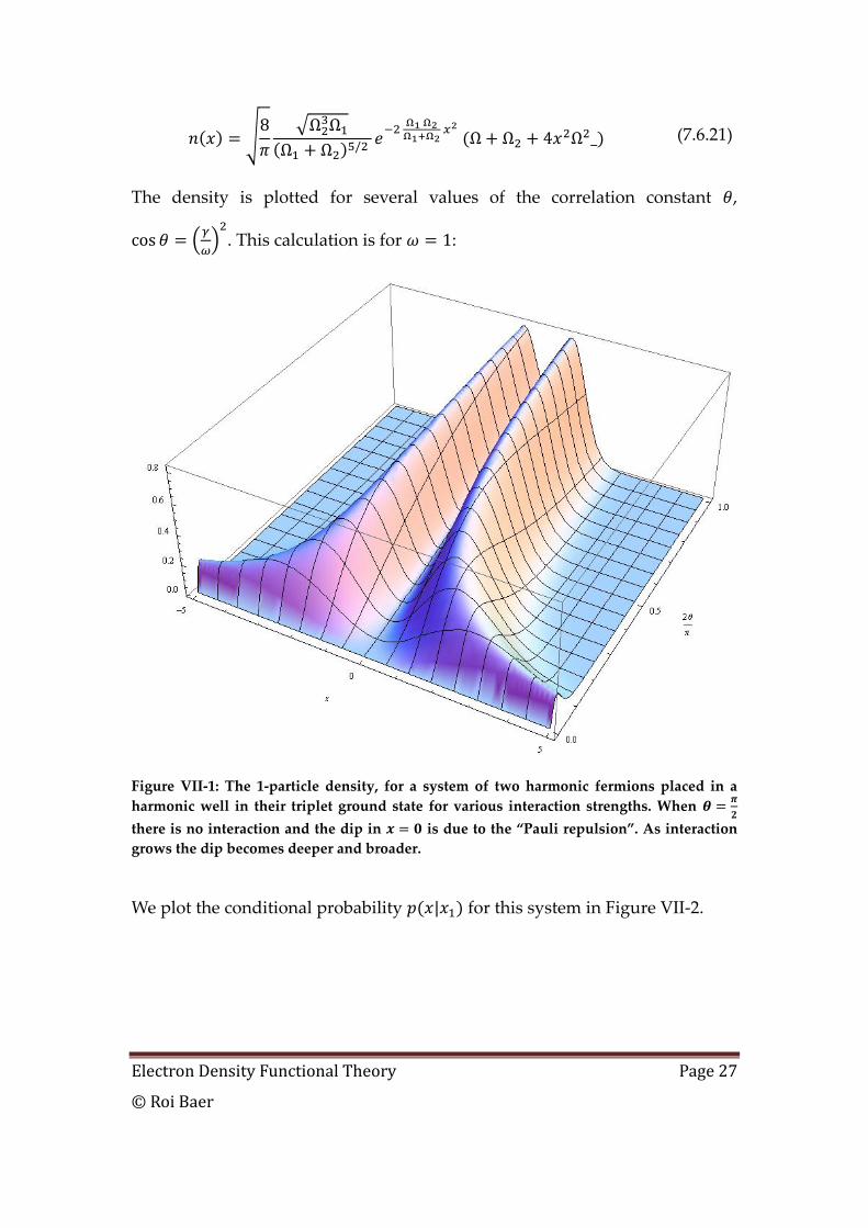
We plot the conditional probability for this system in Figure ‎VII-2.


© Roi Baer

Figure ‎VII-2: Contour plots for the conditional probability distribution for a

system of two Fermions in their triplet ground state for various interaction strengths.

When

there is no interaction and the only correlation is due to the Pauli principle.

As interaction grows the probability distribution rotates by .

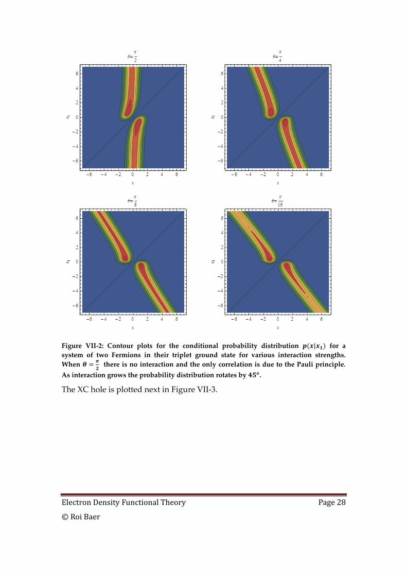
The XC hole is plotted next in Figure ‎VII-3.


© Roi Baer

Figure ‎VII-3: Contour plots for the FC hole for a system of two Fermions in their

triplet ground state for various interaction strengths. When

there is no interaction

and the only correlation is due to the Pauli principle.

iii. The Fermi hole in the non-interacting system

Let us consider now the FC hole in the non-interacting system. Since there is

no correlation in absence of interactions, we attribute the hole only to the

exchange (Fermi) effects. A non-interacting system having the density

that has a closed shell Kohn-Sham determinant, composed of orthonormal

orbitals , where 1 indicates spin up and -1 spin down.


© Roi Baer

(7.6.22)

Where the sum is over the orbitals in (the occupied KS orbitals) and we

defined the density non-interacting matrix .

Exercise: Prove that

(7.6.23)

Exercise: As a check, integrate over and find:

(7.6.24)

The Fermi-conditional density is:

(7.6.25)

And the Fermi-hole is:

(7.6.26)

It can be shown7 that in most cases the density matrix decays

exponentially as , although this could be much slower than .

Thus we may say:

(7.6.27)

This is weaker than Eq. (7.6.16) for the total FC hole. This shows that

decays to zero in a similar but opposite way than


© Roi Baer

(7.6.28)

Based on Eq. (7.6.23) the Fermi hole carries all the charge of the FC hole:

(7.6.29)

This allows one to say that it is the Fermi or “exchange”-hole in the non-

interacting system that “carries the charge” of the exchange correlation-hole

in the interacting system. Once the interacting system has been mapped onto

the non-interacting system the Fermi-hole is easily calculated. This can be

used to define the Coulomb hole by:

(7.6.30)

It has no total charge:

(7.6.31)

The interaction energy can be written now as:

(7.6.32)

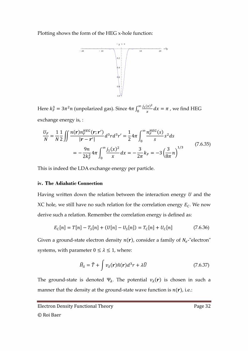
Exercise: Compute the Fermi-hole function of the homogeneous electron gas

Solution: We already determined the density matrix (see Eq.

Error! Reference source not found.)

(7.6.33)

where and

. The x-hole is of course independent

of :

(7.6.34)


© Roi Baer

Plotting shows the form of the HEG x-hole function:

Here (unpolarized gas). Since

, we find HEG

exchange energy is, :

(7.6.35)

This is indeed the LDA exchange energy per particle.

iv. The Adiabatic Connection

Having written down the relation between the interaction energy and the

XC hole, we still have no such relation for the correlation energy . We now

derive such a relation. Remember the correlation energy is defined as:

(7.6.36)

Given a ground-state electron density , consider a family of -"electron"

systems, with parameter , where:

(7.6.37)

The ground-state is denoted . The potential is chosen in such a

manner that the density at the ground-state wave function is , i.e.:

20 10 10 20s kF

1.0

0.8

0.6

0.4

0.2

X s n


© Roi Baer

(7.6.38)

This is a generalization of the idea by Kohn and Sham, that the interacting

electron system is mapped onto a non-interacting electron system with the

same density. Except that now we map our system to a system of electrons

with interaction . When we have the non-interacting system and

is the Kohn-Sham potential and we have:

(7.6.39)

where is the kinetic energy of non-interacting electrons. When we

have the fully interacting system and is the actual external

potential on the electron system and the energy is:

(7.6.40)

We can also define the obvious quantities:

(7.6.41)

From Eq. (7.6.36):

(7.6.42)

With:

Now, the ground-state energy of the intermediately interacting electrons

obeys, by Hellmann-Feynman’s theorem:


© Roi Baer

(7.6.43)

From the second equation then:

(7.6.44)

This expression is the differential form of the adiabatic connection. If we

integrate it with respect to from 0 to 1, we find:

(7.6.45)

This formula is called the "adiabatic connection" formula for the XC energy 8.

We may write: . Then

and so

(7.6.46)

We can rewrite in terms of the correlation hole. Indeed, if , is the

correlation hole for the system then using (7.6.32):

(7.6.47)

From which:

(7.6.48)

And we see that the correlation energy can be obtained from the the -

averaged Coulomb hole, called the correlation hole (since it is associated with

the correlation energy):


© Roi Baer

(7.6.49)

Note that because , we have also:

(7.6.50)

It is interesting that the correlation energy, like to Coulomb energy, can be

represented as a Coulomb interaction of the density and a hole as in Eq.

(7.6.48). Note however that the relevant hole as a coupling-constant ( )

averaged correlation hole and not the Coulomb hole itself.

Let us discuss one of the important consequences of Eq. (7.6.50) i.e. that the

total charge of the correlation hole is zero for localized charge systems. If we

rewrite the correlation energy as:

(7.6.51)

We see that the correlation energy can be written as

(7.6.52)

where:

(7.6.53)

(Note that this is just a suggestion since adding to any function

for which will give the same correlation energy).

Because for a fix is an oveall neutral charge density in space its

“Coulombic potential”

is expected to decay relatively fast for r’(faster

than ).

vii. the kohn-sham method

Documents