wheel slip control in abs brakes using gain scheduled ... · the motivation for an anti-lock...
TRANSCRIPT

Wheel Slip Control in ABS Brakes
using Gain Scheduled Optimal Control
with Constraints
by
Idar Petersen
Thesis submitted for the degree of
Doktor Ingeniør
Department of Engineering Cybernetics
Norwegian University of Science and Technology
Trondheim, Norway
2003

Norwegian University of Science and TechnologyFaculty of Information Technology, Mathematics and Electrical EngineeringDepartment of Engineering CyberneticsN-7491 TrondheimNorway
Dr.ing. thesis 2003:43ITK Report 2003:1-W
ISBN 82-471-5593-1
ISSN 0809-103X

Preface
This thesis is submitted in partial fulfillment of the requirements for thedegree Doktor Ingeniør at the Norwegian University of Science and Tech-nology (NTNU) and is based on research done in the period of February 1998through May 2002.
The doctoral project has been accomplished at SINTEF Automatic Con-trol and the Department of engineering cybernetics, NTNU. My supervisorand coadvisor have been professor Tor A. Johansen and professor BjarneA. Foss respectively. One semester of the doctoral project was spent atthe Department of Electrical Engineering and Computer Science at CaseWestern Reserve University in Cleveland, USA, under the supervision ofprofessor Michael Branicky. The research was sponsored by the EuropeanCommission under the ESPRIT LTR-project 28104 H2C.
Acknowledgments
First and foremost, I would like to thank my advisor professor Tor A. Jo-hansen for his rich source of ideas, practical insight and support throughoutthe entire research. I am grateful for having been given the opportunity towork on an industrial problem within the framework of a doctoral degree.This close co-operation with my supervisor and the industry has resultedin a book chapter, two journals and several conference papers. This H2Cproject and its team dinners will be missed very much.
I would like to acknowledge the cooperative spirit and helpfulness thatI have experienced within the H2C project, specially from Jens Ludemannand Jens Kalkkuhl at DaimlerChrysler.
Sincere thanks go to Dr.Ing. Kai Hofsten and PhD student Petter Tøndelwhom I have been sharing office with. They are duely thanked for theirinsightful comments and for (always) having a twisted view on life in general- there have been some hilarious, non-academic dialogues in that ’think-box-

ii
office’ ! I would also like to thank a former colleague, Dr.Ing. Olav Slupphaugfor his help and ‘Trøndersk’ humour and Dr.Ing. Lars Imsland for ourLMI discussions. I would like to thank all my colleagues and specially themembers of the process control group at NTNU, headed by professor BjarneA. Foss, for an inspiring and social environment.
I am very grateful for the help I have received from Helen Griffiths (fromWales) in proofreading the most important chapters in this thesis.
I would like to thank SINTEF and Sture Holmstrøm for supporting me,and Britt Ottem for all possible help with the administrative paper work.A special thank you to Kjell Eidem for his highly admired service attitudeon unix and other network issues.
I am very grateful for the support from my parents and my extendedfamily, the Brennans, which I had the pleasure to stay with during my sixmonths research period in Cleveland. To my beloved wife, Sobah, who hashelped me with the editing, has always (almost) been kind and supportive,patient and encouraging, and for your patience at my delayed arrivals fordinner and in waiting for me late at night, I dearly love and respect youdeeply. And finally, my dearest daughter Hannah, for all the fantastic mo-ments. If I could only be as awake and happy as you when you wake up inthe middle of the night!
Thank you all, this thesis would never have been possible without yourcontributions.
Idar Petersen
Trondheim, May, 2003

Summary
In a conventional antilock brake system (ABS), the wheel slip will oscillatearound a ”critical slip” within some given thresholds. This oscillation willhave as side effects a noticeable vibration for the driver and limitations inABS performance. Thus, the actual friction force between tyre and roadwill oscillate around a ”maximum” point. The level of complexity presentin current production ABS systems has serious limitations for further devel-opment and analysis.
This thesis looks at the analysis and design of an ABS controller using acontinuously adjustable electromechanical actuator where the ABS aims tocontrol the slip of the wheel to arbitrary setpoints provided by a higher levelcontrol system such as the electronic stability program (ESP). Thus, maxi-mum friction force can be obtained together with a vibration free braking.
This thesis contributes to stability and robustness analysis of a nonlinearABS controller with respect to uncertainty in the road/tyre friction usingLyapunov theory, frequency analysis and experiments with a test vehicle. Acommunication delay between the ABS controller and the electromechanicalactuator together with the actuator dynamics introduce phase losses and theeffect of these performance limitations are also analysed.
This thesis contributes to model-based nonlinear wheel slip controllerdesign, as an explicit gain scheduled LQR design method was used for con-troller design.
Full-scale results are presented for a Mercedes car (E220) equipped witha brake-by-wire system and electromechanical actuators for various test sce-narios, which show that high performance and robustness are achieved. Thetest scenarios consist of straight-line braking on different road surfaces (ice,snow, dry asphalt, wet asphalt and inhomogeneous asphalt/plastic coatedsurface) and a single experiment for braking in a turn on dry asphalt.
The main results of this dissertation have been published in internationaljournals, at international conferences and as a book chapter.

iv

Abbrevations
ABC Active body controlABS Antilock brake systemACC Adaptive cruise controlBAS Brake assist systemBbW Brake by wireBBWM Brake by wire managerCA Collision avoidanceCRC Cyclic redundancy checkDbW Drive by wireEBD Electronic brakeforce distributionECU Electronic control unitEHB Electrohydraulic brakesEKF Extended Kalman filterEMB Electromechanical brakesEMS Electromechanical steeringESP Electronic stability programETC Electronic traction controlHCU Hydraulic control unitISO International Organization for StandardizationLPV Linear parameter-varyingOEM Automotive original equipmentLQR Linear quadratic regulationLQRC LQR with constraintsPM Power managerSAE Society of Automotive EngineersSbW Steer by wireTCS Traction control systemTDMA Time division multiple accessTTP Time-triggered protocol

vi

Contents
1 Introduction 1
1.1 An anti-lock braking system overview . . . . . . . . . . . . . 1
1.2 Literature review . . . . . . . . . . . . . . . . . . . . . . . . . 3
1.3 X-by-Wire . . . . . . . . . . . . . . . . . . . . . . . . . . . . . 5
1.3.1 Electromechanical brakes . . . . . . . . . . . . . . . . 6
1.3.2 The H2C project . . . . . . . . . . . . . . . . . . . . . 9
1.3.3 Requirements for brake-by-wire systems . . . . . . . . 10
1.4 Contributions . . . . . . . . . . . . . . . . . . . . . . . . . . . 11
1.4.1 Model-based nonlinear wheel slip controller design . . 11
1.4.2 Lyapunov stability and robustness analysis . . . . . . 12
1.4.3 Full-scale verification tests . . . . . . . . . . . . . . . . 12
1.4.4 Scope and organization of H2C project . . . . . . . . . 13
1.5 Outline . . . . . . . . . . . . . . . . . . . . . . . . . . . . . . 13
2 Test Vehicle 15
2.1 Computer system and limitations . . . . . . . . . . . . . . . . 15
2.2 Vehicle sensors . . . . . . . . . . . . . . . . . . . . . . . . . . 16
2.2.1 Wheel-speed sensor . . . . . . . . . . . . . . . . . . . . 17
2.3 Electromechanical brake actuator . . . . . . . . . . . . . . . . 18
2.3.1 EMB model . . . . . . . . . . . . . . . . . . . . . . . 19
2.3.2 Actuator dynamics . . . . . . . . . . . . . . . . . . . 22
2.4 TTP Communication . . . . . . . . . . . . . . . . . . . . . . . 23
2.5 Brake-By-Wire-Manager and Power Manager . . . . . . . . . 25
3 Wheel slip dynamics 29
3.1 Wheel slip dynamics . . . . . . . . . . . . . . . . . . . . . . . 29
3.2 Friction modelling . . . . . . . . . . . . . . . . . . . . . . . . 35
3.2.1 Estimation of friction curves . . . . . . . . . . . . . . 37
3.3 Suspension dynamics . . . . . . . . . . . . . . . . . . . . . . 40

viii CONTENTS
4 Gain scheduled wheel slip control 47
4.1 Motivation for gain scheduling . . . . . . . . . . . . . . . . . 47
4.2 Linearized slip dynamics . . . . . . . . . . . . . . . . . . . . . 48
4.3 Wheel slip control design and analysis . . . . . . . . . . . . . 49
4.3.1 Without integral action . . . . . . . . . . . . . . . . . 49
4.3.2 With integral action . . . . . . . . . . . . . . . . . . . 51
4.3.3 With actuator dynamics . . . . . . . . . . . . . . . . . 55
4.4 Discussion . . . . . . . . . . . . . . . . . . . . . . . . . . . . . 60
5 Implementation, redesign and tuning 65
5.1 Controller structure . . . . . . . . . . . . . . . . . . . . . . . 65
5.2 ABS supervisory logic . . . . . . . . . . . . . . . . . . . . . . 66
5.3 Controller states . . . . . . . . . . . . . . . . . . . . . . . . . 67
5.4 LQR with input and state constraints . . . . . . . . . . . . . 68
5.4.1 Overview . . . . . . . . . . . . . . . . . . . . . . . . . 68
5.4.2 Brief introduction to LQRC design theory . . . . . . . 69
5.4.3 Structure of the LQRC solution . . . . . . . . . . . . . 71
5.4.4 State space partitioning . . . . . . . . . . . . . . . . . 72
5.4.5 Computational strategies . . . . . . . . . . . . . . . . 72
5.5 ABS specifications for LQRC design . . . . . . . . . . . . . . 73
5.5.1 Gain scheduling control . . . . . . . . . . . . . . . . . 73
5.5.2 System and cost function specifications . . . . . . . . 74
5.5.3 Constraint specifications . . . . . . . . . . . . . . . . . 75
5.5.4 Constraint handling . . . . . . . . . . . . . . . . . . . 75
5.6 Frequency response analysis . . . . . . . . . . . . . . . . . . 76
5.7 Improvement of initial transient response . . . . . . . . . . . 78
5.7.1 Controller initialization . . . . . . . . . . . . . . . . . 79
5.7.2 Off-equilibrium scheduling on slip . . . . . . . . . . . . 79
5.8 Bumpless transfer due to controller switching (gain schedul-ing) . . . . . . . . . . . . . . . . . . . . . . . . . . . . . . . . 80
5.9 Anti-windup . . . . . . . . . . . . . . . . . . . . . . . . . . . . 80
6 Experimental Results 83
6.1 Experimental scenarios . . . . . . . . . . . . . . . . . . . . . . 83
6.2 Presentation of experimental results . . . . . . . . . . . . . . 84
6.3 Wet inhomogeneous surface . . . . . . . . . . . . . . . . . . . 85
6.3.1 Slip . . . . . . . . . . . . . . . . . . . . . . . . . . . . 85
6.3.2 Lateral stability . . . . . . . . . . . . . . . . . . . . . 86
6.3.3 Deceleration of vehicle . . . . . . . . . . . . . . . . . . 86
6.3.4 Friction estimate . . . . . . . . . . . . . . . . . . . . . 86

CONTENTS ix
6.3.5 Controller performance . . . . . . . . . . . . . . . . . 866.4 Dry asphalt . . . . . . . . . . . . . . . . . . . . . . . . . . . . 86
6.4.1 Slip . . . . . . . . . . . . . . . . . . . . . . . . . . . . 866.4.2 Lateral stability . . . . . . . . . . . . . . . . . . . . . 866.4.3 Deceleration of vehicle . . . . . . . . . . . . . . . . . . 926.4.4 Friction estimate . . . . . . . . . . . . . . . . . . . . . 926.4.5 Controller performance . . . . . . . . . . . . . . . . . 92
6.5 Wet asphalt . . . . . . . . . . . . . . . . . . . . . . . . . . . . 926.5.1 Slip . . . . . . . . . . . . . . . . . . . . . . . . . . . . 926.5.2 Lateral stability . . . . . . . . . . . . . . . . . . . . . 926.5.3 Deceleration of vehicle . . . . . . . . . . . . . . . . . . 956.5.4 Friction estimate . . . . . . . . . . . . . . . . . . . . . 956.5.5 Controller performance . . . . . . . . . . . . . . . . . 95
6.6 Snow . . . . . . . . . . . . . . . . . . . . . . . . . . . . . . . . 956.6.1 Slip . . . . . . . . . . . . . . . . . . . . . . . . . . . . 956.6.2 Lateral stability . . . . . . . . . . . . . . . . . . . . . 956.6.3 Deceleration of vehicle . . . . . . . . . . . . . . . . . . 996.6.4 Friction estimate . . . . . . . . . . . . . . . . . . . . . 996.6.5 Controller performance . . . . . . . . . . . . . . . . . 99
6.7 Ice . . . . . . . . . . . . . . . . . . . . . . . . . . . . . . . . . 996.7.1 Slip . . . . . . . . . . . . . . . . . . . . . . . . . . . . 996.7.2 Lateral stability . . . . . . . . . . . . . . . . . . . . . 996.7.3 Deceleration of vehicle . . . . . . . . . . . . . . . . . . 996.7.4 Friction estimate . . . . . . . . . . . . . . . . . . . . . 1036.7.5 Controller performance . . . . . . . . . . . . . . . . . 103
6.8 Turning on dry asphalt . . . . . . . . . . . . . . . . . . . . . . 1036.8.1 Slip . . . . . . . . . . . . . . . . . . . . . . . . . . . . 1036.8.2 Lateral stability . . . . . . . . . . . . . . . . . . . . . 1036.8.3 Deceleration of vehicle . . . . . . . . . . . . . . . . . . 1096.8.4 Friction estimate . . . . . . . . . . . . . . . . . . . . . 1096.8.5 Controller performance . . . . . . . . . . . . . . . . . 109
6.9 Dry asphalt, controller initialization . . . . . . . . . . . . . . 1096.9.1 Slip . . . . . . . . . . . . . . . . . . . . . . . . . . . . 1096.9.2 Lateral stability . . . . . . . . . . . . . . . . . . . . . 1136.9.3 Deceleration of vehicle . . . . . . . . . . . . . . . . . . 1136.9.4 Friction estimate . . . . . . . . . . . . . . . . . . . . . 1136.9.5 Controller performance . . . . . . . . . . . . . . . . . 113
6.10 Dry asphalt, off-equilibrium design . . . . . . . . . . . . . . . 1136.10.1 Slip . . . . . . . . . . . . . . . . . . . . . . . . . . . . 1176.10.2 Lateral stability . . . . . . . . . . . . . . . . . . . . . 117

x CONTENTS
6.10.3 Deceleration of vehicle . . . . . . . . . . . . . . . . . . 1176.10.4 Friction estimate . . . . . . . . . . . . . . . . . . . . . 1176.10.5 Controller performance . . . . . . . . . . . . . . . . . 117
6.11 Experimental problems . . . . . . . . . . . . . . . . . . . . . . 117
7 Conclusions 1197.1 Future works . . . . . . . . . . . . . . . . . . . . . . . . . . . 121
A Explicit Sub-optimal Linear Quadratic Regulation with Stateand Input Constraints 131A.1 Introduction . . . . . . . . . . . . . . . . . . . . . . . . . . . . 131A.2 Controller decomposition . . . . . . . . . . . . . . . . . . . . 134
A.2.1 Active constraint set sequences . . . . . . . . . . . . . 134A.2.2 Decomposition of the HJB equation . . . . . . . . . . 136
A.3 Computing gain matrices . . . . . . . . . . . . . . . . . . . . 139A.4 State space partitioning . . . . . . . . . . . . . . . . . . . . . 143
A.4.1 Activity region . . . . . . . . . . . . . . . . . . . . . . 143A.4.2 Outer Approximations to the Activity Regions . . . . 145A.4.3 Partitioning Algorithm . . . . . . . . . . . . . . . . . . 149
A.5 Optimality, complexity and real-time implementation . . . . . 151A.5.1 Upper and lower bounds on cost function . . . . . . . 151A.5.2 Complexity reduction by sub-optimality . . . . . . . . 151A.5.3 Real-time Implementation . . . . . . . . . . . . . . . . 153
A.6 Conclusions . . . . . . . . . . . . . . . . . . . . . . . . . . . . 156
B Details of Proof 159

Chapter 1
Introduction
”Braking is to be done as hard and late as possible to ensure thatyour ABS kicks in, giving a nice, relaxing foot massage as thebrake pedal pulsates. For those of you without ABS, it’s a chanceto stretch your legs.” Unknown
The motivation for an anti-lock braking system (ABS) is that it canprovide improvements in the performance of the vehicle under braking com-pared to a conventional brake system (SAE 1992). Performance improve-ment is typically sought in the areas of stability, steerability and stoppingdistance. An ABS controls the slip of each wheel to prevent it from lockingsuch that a high friction is achieved and steerability is maintained. ABScontrollers are characterized by robust adaptive behaviour with respect tohighly uncertain tyre characteristics and fast changing road surface proper-ties (SAE 1992; Burckhardt 1993).
This chapter gives an overview of ABS (history and its function), fol-lowed by a literature review on ABS controllers. To prepare the readerfor the research presented in this thesis, information on x-by-wire and elec-tromechanical brakes is then provided. This chapter ends with a summaryof the contributions found in this thesis, together with the layout of thisthesis.
1.1 An anti-lock braking system overview
The current hydraulic ABS systems were conceived from systems developedfor trains in the early 1900’s. Next, anti-lock brakes were developed to assistaircrafts stop straight and quickly on slippery runways. In 1947, the first

2 Introduction
use of anti-lock brakes on aeroplanes was on B-47 bombers to avoid tireblowout on dry concrete and spin-outs on icy runways. The first automotiveuse of ABS was in 1954 on a limited number of Lincolns which were fittedwith an ABS from a French aircraft. In the late 60’s, Ford, Chrysler, andCadillac offered ABS on very few models. These very first systems usedanalog computers and vacuum-actuated modulators. Since the vacuum-actuated modulators cycled so slowly, the vehicle’s actual stopping distanceincreased. Legal concerns then literally put the development on hold in theUS, while the European companies took the lead in the next 10-20 years. Inthe late 70’s, Mercedes and BMW introduced electronically-controlled ABSsystems. By 1985, Mercedes, BMW and Audi had introduced Bosch ABSsystems and Ford introduced its first Teves system. By the late-80’s, ABSsystems were offered on many high-priced luxury and sports cars. Today,braking systems on most passenger cars and many light-duty vehicles havebecome complex, computer-controlled systems. Since the mid-80’s, vehiclemanufacturers have introduced dozens of anti-lock braking systems. Thesesystems differ in their hardware configurations as well as in their controlstrategy (SAE 1992; Burckhardt 1993).
Any production ABS incorporates a number of subsystems and in mostABS systems there will be a slip controller subsystem, the objective of whichis to avoid locking the wheels under a braking manoeuvre, either by ensuringthat the slip stays within a specified range or at a given setpoint. Notethat not all ABS systems estimate and control the wheel slip explicitly, butwork on speed and acceleration instead. Among these subsystems, the logicresponsible for coordinating the four wheel slip controllers is of particularimportance. The wheel slip controllers for each wheel are (as safety devices)only active in critical situations. Thus, each controller is switched off andthe brake is set to manual operation when the wheel is no longer in dangerof being locked. On the other hand, the slip controller has to be switchedon early enough to prevent the wheel from locking. Thus, the correspondingswitching logic is crucial for the functionality of the ABS.
The basic control-philosophy (Burckhardt 1993; Hattwig 1993; Maisch,Mergenthaler, and Sigi 1993; Maier and Muller 1995; Wellstead and Pettit1997) for conventional ABS systems, is a combination of
• slip control and
• wheel acceleration control.
Wheel acceleration control uses the measured wheel angular velocitiesto control indirectly the slip by regulating the acceleration/decelration of

1.2 Literature review 3
the wheels. The actuator used in conventional ABS systems is a hydraulicsolenoid valve which has three brake pressure modes:
• increase
• hold
• reduce
The controller is switched on when the deceleration of the wheel dropsbelow a specified value for a given period of time. As long as the ABS isactive, the switching between the different actuator modes (increase, holdor reduce) is controlled either using several slip and acceleration thresholdsor by defining a switching surface using a weighted sum of slip and accel-eration. By appropriately selecting these thresholds, the slip will oscillatearound the “critical slip”. Thus, the friction force between the tyres and theroad surface will be close to its maximum value and the braking distanceis minimized. This kind of algorithm will have vibrations as a side effectwhich are noticeable while braking (Burckhardt 1993).
Slip control works satisfactorily for non-decreasing tyre force character-istics while wheel acceleration control tends to work better for tyre charac-teristics which have a pronounced maximum. This is due to the fact thata larger wheel acceleration/deceleration can be obtained in the pronouncedmaximum case. ABS controllers have been shown to be highly adaptivesince they can tolerate a considerable amount of uncertainty in the tyreforce characteristics and the friction coefficient.
Conventional ABS systems have some limitations in control and per-formance. One of the most significant disadvantages of these systems istheir disability in slip control and tracking of a specified desired slip in anacceptable range.
Today’s production ABS is a rule-based control system that has exhaus-tive tables for different braking scenarios. The controllers are tuned in atrial and error manner using simulations and exhaustive field testing. Thelevel of complexity of these systems is a serious limitation for the analysisand further development of the current production ABS systems.
1.2 Literature review
Different control methods have been tested for their performance in ABS.The model-based approach in (Drakunov, Ozguner, Dix, and Ashrafi 1995)

4 Introduction
applies a search for the optimum brake torque via sliding modes. This ap-proach requires the tyre force, hence, a sliding observer is used to estimateit. The approach is tested in a simplified simulation environment. Slidingmode control has been tested in a hardware in the loop simulator (Kawabe,Nakazawa, Notsu, and Watanabe 1997) and also in a vehicle. A derivativepart depending on the rotational acceleration is introduced in order to re-duce the chattering of the sliding controller. The sliding controller proposedby (Choi and Cho 1998) is mainly used to show the advantage of a PWMcontrolled actuator. (Wu and Shih 2001) design an ABS controller (with-out slip-feedback) which integrates sliding-mode control with PWM. Slidingmode control is also considered in (Schinkel and Hunt 2002).
Another theoretical approach is presented by (Freeman 1995). Freemandesigns an adaptive Lyapunov-based nonlinear wheel slip controller. Thiscontroller has been extended in (Yu 1997) by introducing speed dependenceof the Lyapunov function and also including a model of the hydraulic cir-cuit dynamics. Neither of these two latter approaches have been tested insimulation or in a real vehicle. Another Lyapunov based nonlinear adaptivetyre slip controller is presented in (Ludemann 2002) using Sontag’s formula(Sontag 1989; Krstic, Kanellakopoulos, and Kokotovic 1995). No actuatordynamics have been included in this analysis.
Feedback linearization to design a slip controller is suggested by (Liuand Sun 1995) where gain scheduling is used to handle the variation of thetyre friction curve with respect to speed.
A maximum tyre/road friction approach using optimal control theory isproposed in (Tsiotras and Canudas de Wit 2000) based on a static frictionmodel.
An adaptive emergency braking controller designed to achieve near-maximum braking effort is suggested in (Yi, Alvarez, Horowitz, and Canudasde Wit 2000).
(Wellstead and Pettit 1997) formulate a conventional ABS controller asa piecewise linear controller including analysis of the switching cycles. Inves-tigations on a variable desired slip can be found in (Fajdiga and Janicijevic1992). The desired slip is varied according to the side slip angle.
(Taheri and Law 1991) design a simple PD wheel slip controller by theZiegler-Nichols rule, focusing on the desired slip value. The desired slip isestimated by evaluating the switching of a conventional ABS. Additionally,a modification of the desired slip according to the steering angle is alsoproposed.
A robust PID controller based on loop-shaping and a nonlinear PID,where the nonlinear function gives a low/high gain for large/small errors

1.3 X-by-Wire 5
respectively, are proposed in (Jiang 2000) together with simulation resultsfor a heavy vehicle. Other PID-type approaches to wheel slip control areconsidered in (Jun 1998; Wang, Schmitt-Hartmann, Schinkel, and Hunt2001; Solyom and Rantzer 2002).
Conventional ABS control is compared against PID, sliding and fuzzycontrollers in (Jun 1998). The PID algorithm adapts very slowly on differentroad surfaces. A combination of the model-based approaches should givegood performance; but this has not been tested.
1.3 X-by-Wire
There is an increasing demand on automotive original equipment manufac-turers (OEM) to increase vehicle safety and performance, while simultane-ously reducing manufacturing costs and maximizing efficiencies in the designprocess (Leen and Heffernan 2002). The introduction of x-by-wire (XBW)systems into the automotive environment is gaining rapid momentum, andXBW examines the global movement toward replacing hydraulics and me-chanical systems with electronics for safety-critical applications. The ”x” in”x-by-wire” represents the basis of any safety-related application, such assteering, braking, power train, suspension, throttle control or multi-airbagsystems. These applications aim to increase overall vehicle safety and per-formance by liberating the driver from routine tasks and assisting the driverto find solutions in critical situations.
Integrating by-wire systems will create both functional and infrastruc-ture improvements. Functional improvements include (Delphi 2002):
• Improved ride and handling - By-wire computer control of chassis dy-namics allows steering, braking, and suspension to work together.
• Enhanced stability control - Sensors and controllers work together todetect then correct increased yaw movements that could result in spin-outs or rollovers.
• Safety-enhancing systems - By-wire technology provides the commu-nication link necessary to enable safety systems like lane keeping andcollision avoidance.
Through modular design and the elimination of hardware, x-by-wire of-fers several infrastructure improvements (Delphi 2002):
• Increased modularity - Fully functional by-wire modules reduce OEMassembly time and cost.

6 Introduction
• Improved driver interface - The elimination of mechanical connectionsto the steering column gives OEMs more flexibility in designing thedriver interface with regard to location, type, feel, and performance.
• Enhanced passive safety - An x-by-wire cockpit can simplify and im-prove occupant restraint management.
• Added flexibility - Vehicle designers will have more flexibility in theplacement of hardware under the hood and in the interior to supportalternative powertrains, enhance styling and improve interior function-ality.
• Lead-time reduction - OEMs will be able to use a laptop computerto perform soft tuning capabilities instead of manually adjusting me-chanical components.
The following paragraph has been extracted from (Leen and Heffernan2002). In the past few years there has been a tendency in vehicle construc-tion to increase the safety of vehicles by introducing intelligent assistancesystems (e.g. ABS, Brake-Assistant (BA), Electronic Stability Program(ESP), etc.) that help the driver to cope with critical driving situations.Typical for these functions is the active control of the driving dynamics bydistributed assistant systems, which therefore need a communication net-work. The electronic components which control these functions are safety-critical. However, the assistance functions deliver only an add-on service inaccordance to a fail-safe strategy for the electronic components. If there isany doubt about the correct behavior of the assistance system, it will be shutdown. For by-wire systems without a mechanical backup, a new dimensionof safety requirements for automotive electronics is reached. After a fault,the system has to be fail-operational until a safe state (e.g. vehicle standstill) is reached.
Figure 1.1 shows how dynamic driving-control systems have been steadilyadopted since the 1920’s.
1.3.1 Electromechanical brakes
Brake-by-wire means that there is no hydraulic or mechanical connection be-tween the brake pedal and the brake actuators. The driver’s brake commandresults in an electrical signal that is communicated via micro-controllers tothe actuator. Such technologies require new types of brake actuators such aselectromechanical, (Hedenetz and Belschner 1998; Schwarz 1999; Isermann,

1.3 X-by-Wire 7
1924
1931
1937
1951
1952
1963
1978
1989
1994
1995
1998
>2002
Mechanical
Hydraulic
Eletcronic
Dynamic Driving Control
Bra
ke-b
y-w
ire
Modified source: Computer, January 2002
0% 100%
Tim
e (
nonlinear)
Incre
ased D
ependency o
n E
lectr
onic
s
ABS Antilock brake systemACC Adaptive cruise controlEBD Electronic brakeforce distributionECU Electronic control unitEHB Electrohydraulic brakesEMB Electromechanical brakesESP Electronic stability programHCU Hydraulic control unit
Researchpotential
ABS
ABS+TCS
ABS/EBD
ESP
ACC
EHB
EMB
Hydraulic
2 circuits
TCM
Disk brakes
Vacuumboost
Hydraulicboost
Sensors ECU HCU
Sensors ECU HCU
Sensors ECU HCU
Sensors ECU HCU
Sensors ECU
Sensors HCUECU
Sensors ActuatorECU
HCU
Mechanical
Figure 1.1: Past and projected progress in dynamic driving control systems.
Schwarz, and Stolzl 2002), or electro-hydraulic brakes. A main feature ofelectromechanical and electro-hydraulic brakes compared to conventionalbrakes with solenoid valves is that they allow accurate continuous adjust-ment of the brake force.
Electromechanical Braking systems (EMB), also referred to as brake-by-wire, takes the place of conventional hydraulic braking systems witha completely ‘dry’ electrical component system by replacing conventionalactuators with electric motor-driven units. EMB is designed to improveconnectivity with other vehicle systems, thus enabling simpler integrationof higher level functions such as traction control (ETS), acceleration skidcontrol (ASR), ESP and BA. This integration may vary from embeddingthe function within the EMB system, as in ABS, to interfacing to theseadditional systems using communication links.
This move to electronic control helps to eliminate many of the manufac-

8 Introduction
turing, maintenance, and environmental concerns associated with hydraulicsystems. The potential benefits of the EMB systems include:
• Assistance functions (ABS, BA, ESP,...) which could be realized bysoftware and sensors, and without additional mechanical or hydrauliccomponents.
• Benefit due to electrical interfaces instead of hydraulic interfaces, whichallow easier adapting of assistance systems.
• A reduction in system weight resulting in improved vehicle perfor-mance and economy.
• Simpler maintenance as maintenance requirements are reduced.
• Ecological as there is a reduction in pollutant sources reduction throughthe elimination of corrosive and toxic hydraulic fluids.
• Comfort as pedal ergonomics are adaptable.
• Nearly rest torque-free.
• No mechanical links between the brake components and the enginecompartment, improving passive safety.
• No perceptible noise emission when braking.
• Reduced costs for assembly during line production due to simpler andfaster assembly of the system into the host vehicle.
• Intelligent error response
• The supervisory monitoring system will not interfere with the pedalmovement (no pulsating effect felt).
• Implementation of features such as ‘hill hold’.
Another advantage is the elimination of the large vacuum booster foundin conventional systems which helps simplify the production of right andleft-hand drive vehicle variants.
To satisfy the fail-operational requirement, an additional redundancy inthe control components, sensors, software, power supply and the communi-cation system has to be included. Nevertheless, there are still good reasons(as listed above) to introduce by-wire functions for brake systems.

1.3 X-by-Wire 9
As mentioned earlier, production ABS uses the wheel acceleration tocontrol the slip to maximize the friction force. In the next generation ofbrake-by-wire systems where EMB’s are used, it may be beneficial to in-troduce a shift from wheel acceleration/deceleration control to slip setpointcontrol. The slip setpoint is supposed to be provided by a higher level con-trol system (e.g. ESP) which can be used to stabilize the lateral dynamicsof the vehicle while braking. In this way, the control objective is shifted tomaintain a specified slip for each of the vehicle’s wheels. This makes wheelslip control an interesting alternative to conventional ABS systems, wherethe control logic usually does not include an explicit wheel slip controller(SAE 1992; Maier and Muller 1995; Wellstead and Pettit 1997). The targetslip may also be based on automatic monitoring of the road conditions, e.g.(Gustafsson 1997).
1.3.2 The H2C project
Heterogenous Hybrid Control (H2C) is an European Commission ESPRITLTR-project which was started in late 1998 consisting of participants fromDaimlerChrysler (Germany), Glasgow University (Scotland), Lund Univer-sity (Sweden) and SINTEF (Norway). One major research part of theproject was to study wheel slip control for an ABS system, where Daim-lerChrysler provided a vehicle (a Mercedes E220) fitted with EMB. Thefollowing paragraph describes briefly the methods used in designing wheelslip controllers by the project participants in the H2C project.
The electro-mechanical wheel brake by Continental Teves (Schwarz 1999;Ludemann 2002) is a disk brake working on the floating caliper-principle.(Ludemann 2002) formulates two possible hybrid ABS controllers: a Lyapunov-based nonlinear PI-type controller and a nonlinear adaptive slip control us-ing Sontag’s formula (Sontag 1998; Krstic, Kanellakopoulos, and Kokotovic1995) which both have been tested. (Schinkel and Hunt 2002) formulatean ABS control using a sliding mode approach. A linearization of a non-linear model is used in (Wang, Schmitt-Hartmann, Schinkel, and Hunt 2001),where a SSP(simultaneous stabilisation problem) approach is used to designan ABS controller. In (Solyom and Rantzer 2002), a model-based designmethod for gain scheduled robust nonlinear PI(D) controllers is describedand tested. It should be noted that the controller performance by the differ-ent controller design methods implemented and tested in the H2C project,were shown to converge by the end of the project (Ludemann 2002), but arenot conclusive. This is due to the fact that there are no scenarios containingcomplete test data for well-tuned controllers.

10 Introduction
There are several more producers of electromechanical brake actuatorsfrom companies such as Siemens, Delphi, Lucas, Bosch, Honda. Due tothe industrial property rights and very strict proprietary policies withinthe automotive industry, very little has been published around automotiveEMB. There is no literature describing tests and performance results of EMBbeside those that have been carried out through the H2C project.
1.3.3 Requirements for brake-by-wire systems
There are several requirements for brake-by-wire systems, which are listedbelow (the terms Safety, Reliability, Maintainability and Availability areused in accordance with the definition of (Laprie 1995)). First, some com-mon requirements for automotive by-wire systems (Hedenetz and Belschner1998):
• Safety - after one arbitrary fault, the system must be available in asatisfying manner e.g., the brakes have to work with an adequate brakeforce.
• Reliability - the reliability of a by-wire system must be at least as highas a comparable mechanical system.
• Availability - the availability must be at least as high as present sys-tems.
• Maintainability - the maintainability intervals must be at least as longas present systems.
• Lifetime - the lifetime must be at least as long as present systems.The Society of Automotive Engineers (SAE) classified in-vehicle com-munication systems into three categories, class A-C (SAE 1993). Forsafety-related communication systems, class C is required.
• Costs - must be not more than to those of conventional systems.
• Compartment - must be small enough for easy integration of the com-ponents.
• Legal aspects - must be fulfilled (Council 1971) (EU has set toleranceguidelines for brake systems. When the braking performance fallswithin these tolerance levels, the system is considered safe).
Then, the special requirements for brake-by-wire systems:

1.4 Contributions 11
• Actuators - the brake actuator must be free of braking torque in caseof power loss.
• Sensors - triple redundancy shall be used for the pedal sensors to getone valid pedal measurement by the loss of one sensor.
• Power supply - two independent power supplies must be used.
• Communication - the communication system must be fail-operationalafter one fault.
• Software - the software must be certified (eg. ISO).
To reach these requirements, new technologies had to be developed forthe actuators (Schwarz 1999; Ludemann 2002), communication (FlexRay2002; Hedenetz and Belschner 1998; Kopetz and Grunsteidl 1994) and elec-tronic components (Flemming 2001; Leen and Heffernan 2002).
1.4 Contributions
The introduction of advanced functionality such as ESP, drive-by-wire andmore sophisticated actuators and sensors offers both new opportunities andrequirements for a higher performance in ABS brakes. The main motivationfor this research has been to analyze and design an ABS controller on anautomotive vehicle fitted with a new electromechanical actuator, rather thana hydraulic actuator, which allows continuous adjustment of the clampingforce. The main contributions of this thesis can be summarized as:
• Model-based nonlinear wheel slip controller design.
• Lyapunov stability and robustness analysis.
• Full-scale verification tests.
1.4.1 Model-based nonlinear wheel slip controller design
The wheel slip dynamics are highly nonlinear. Despite this, the wheel slipcontroller design used in this research work is based on an explicit linearquadratic regulation (LQR) design method developed recently, which takesinto account the input and state constraints (Johansen, Petersen, and Slup-phaug 2000a; Johansen, Petersen, and Slupphaug 2002). The control design

12 Introduction
relies on local linearization and gain scheduling. My contribution to the de-sign method is mostly on the implementation and the verification of the de-sign method. Two modifications were developed and tested which improvedthe initial transient response: controller initialization and off-equilibriumdesign. This constrained LQR will hereafter be referred to as LQRC. Thefull paper (Johansen, Petersen, and Slupphaug 2002), that describes thecontroller design method LQRC, is included in Appendix A. In addition,a MATLAB toolbox was developed for the LQRC controller design method(Johansen and Petersen 2001).
Proceeding results were reported in (Branicky, Johansen, Petersen, andFrazzoli 2000; Johansen, Kalkkuhl, Ludemann, and Petersen 2001).
1.4.2 Lyapunov stability and robustness analysis
As the control design relies on local linearization and gain scheduling, the ef-fects of this simplification are analyzed with a somewhat idealized Lyapunov-based nonlinear stability and robustness analysis, taking into account un-certain tyre friction nonlinearities. The Lyapunov function is derived usingthe Riccati equation solution. Robust stability is shown for a wide range ofslip, tyre friction and expected speed values (Petersen, Johansen, Kalkkuhl,and Ludemann 2001; Petersen, Johansen, Kalkkuhl, and Ludemann 2002).
In order to also investigate the effects of sampling, communication delays,actuator dynamics and the fundamental limitations in performance, thisanalysis is complemented by a classical frequency analysis in (Johansen, Pe-tersen, Kalkkuhl, and Ludemann 2003). The model used in the three previ-ous references has been extended to include actuator dynamics in (Petersen,Johansen, Kalkkuhl, and Ludemann 2003). Here, a parameter-dependentLyapunov function for the nominal closed loop was found by solving anlinear matrix inequality (LMI) problem and this function was used to inves-tigate the robustness with respect to uncertainty in the road/tyre frictioncharacteristic. Lyapunov stability and robustness analysis are treated inChapter 4.
1.4.3 Full-scale verification tests
This research work contains detailed experimental evaluation using a testvehicle, a Mercedes E220, provided by DaimlerChrysler. The test resultsincluded in this thesis are from a series of successful experiments carriedout for a straight-line braking manoeuvre on different road surfaces (ice,snow, dry asphalt, wet asphalt and inhomogeneous asphalt/plastic coated

1.5 Outline 13
surface) and braking in a turn on dry asphalt. The results have in part beenpublished in (Petersen, Johansen, Kalkkuhl, and Ludemann 2001; Petersen,Johansen, Kalkkuhl, and Ludemann 2002; Johansen, Petersen, Kalkkuhl,and Ludemann 2003; Petersen, Johansen, Kalkkuhl, and Ludemann 2003)and are analyzed in Chapter 6.
1.4.4 Scope and organization of H2C project
The LQRC controller design method was chosen by the H2C project as themethod seemed promising with respect to handling input and state con-straints. Half-way through the project, the test vehicle was fitted with anew and faster electromechanical brake-actuator. As a consequence of thisupgrade, the need for a design method handling constraints became lessimportant.
The H2C project was organized such that the test vehicle was providedby DaimlerChrysler with their software and hardware implementations. Animportant issue to mention is that the extended Kalman-filter was providedby DaimlerChrysler. Time was spent on software programming for basicsupport function like controller logging and making the application softwareflexible to allow toggling of active controller and setting of parameters on-line without requiring a recompilation of the run-time software code. Themain software provided by the other project participants was their respectivewheel slip controller.
DaimlerChrysler also provided a vehicle simulator and a tyre frictionmodel. The simulator was used extensively for thorough testing of the wheelslip controller before being implemented into the test vehicle.
1.5 Outline
Chapter 2 gives an overview of the vehicle with its sensors and computersystem. In addition, to provide an insight into the fault toleranceand safety of the ABS used, descriptions of the TTP communicationand the brake-by-wire-/power-manager are given. A detailed descrip-tion of the state-of-the-art electromechanical brake actuator and itsdiscretized model are also included.
Chapter 3 presents the wheel slip dynamics and the quarter car model.Friction curves are presented showing the variation of tyre/road fric-tion as a function of wheel slip for various road conditions. Thischapter also gives an introduction to friction modelling together with

14 Introduction
estimation of friction curves based on experimental data. Finally, dy-namics caused by the vehicle pitching is discussed.
Chapter 4 describes why gain scheduled control is suitable for ABS controland presents a linearization of wheel slip dynamics and its properties.Gain scheduled LQ designs with Lyapunov analysis for three cases areprovided: (i) slip dynamics without integral action, (ii) slip dynam-ics with integral action, (iii) slip dynamics with integral action andactuator dynamics.
Chapter 5 explains the implementation, redesign and tuning of the wheelslip controller. An overview of the controller structure, the ABS su-pervisory logic and the controller states is given. An introduction isthen given to the controller design method, LQRC, and its constraintspecification. A further analysis of the effects of choice of slip setpoint,sampling, communication delays, actuator dynamics and performancelimitations is provided by a classical frequency analysis. Two redesignsthat improved the initial transient response (controller initializationand off-equilibrium design) are described. The implementation of anti-windup and bumpless transfer due to gain switching are described indetail.
Chapter 6 describes and discusses in detail all test scenarios and test re-sults that have been conducted. Straight-line braking manoeuvres areshown for surfaces like ice, snow, dry asphalt, wet asphalt and onan inhomogeneous asphalt/plastic coated surface. Experiments wherebraking was carried out while turning on dry asphalt and the verifica-tion of improved initial transient responses are also shown.
Chapter 7 provides discussion and conclusions of this research.
Appendix A is a reprint of (Johansen, Petersen, and Slupphaug 2002).
The notation is consistent throughout the thesis.

Chapter 2
Test Vehicle
This chapter briefly states the computer system used in the vehicle and aconcise functional overview of relevant sensors. An extensive description ofthe EMB, its dynamics and limitations are provided. Further, a brief insightinto the TTP communication, the brake-by-wire manager (BBWM) and thepower manager/supply unit (PM) are also provided as to explain the safetyaspects and why there are inherent physical limitations imposed on the ABScontroller bandwidth.
The experimental vehicle is a Mercedes E220 equipped with four elec-tromechanical disk brake actuators supplied by Continental Teves and abrake-by-wire system. Figure 2.1 shows a photo of the test vehicle.
2.1 Computer system and limitations
Figure 2.2 shows the hardware architecture of the vehicle. It consists of fourservo controllers for the brakes, a monitoring unit, a BBWM and a PM.These systems communicate via a TTP (time-triggered protocol) bus andthe main computer system (for BBWM) consisted of a Motorola 68060 CPUwith a floating-point coprocessor. Three major system limitations are listedbelow having a direct impact on the ABS controller:
i. Limited available processing capacity by the BBWM-CPU for con-troller processing. This limitation is mainly due to the extendedKalman filter, which required most of the CPU’s processing capac-ity.
ii. Limited available memory for applications running on BBWM. Thishas a directly limitation on how large the ABS controller software can

16 Test Vehicle
Figure 2.1: The experimental vehicle
be.
iii. Phase losses are introduced by the TTP communication delay betweenthe BBWM and the electronic control unit (ECU). This imposes fun-damental performance limitations.
2.2 Vehicle sensors
The vehicle is equipped with the following sensors:
• Four wheel speed sensors.
• A sensor for the steering wheel angle.
• Sensors for the position of the brake pedal and the force applied tothe brake pedal.
• Two accelerometers for longitudinal and lateral acceleration respec-tively.
• A yaw rate sensor.

2.2 Vehicle sensors 17
Power Supply(Manager)
Brake-by-WireManager
Communi-cation Unit
Monitoringand
Diagnosis
BrakeECU
BrakeECU
BrakeECU
BrakeECU
Figure 2.2: Diagram of test vehicle with brake-by-wire
• Four Hall sensors for measuring the clamping forces at each brake.
To determine the driver’s intent, the information about the angle ofthe steering wheel is needed, which is typically delivered from a variable-photosensitivity wheel that interrupts a light beam.
Several sensors are used to track the actual vehicle response to thedriver’s inputs. Vehicle speed can be estimated from the anti-lock brakewheel-speed sensors. The on-board computer makes an estimate of the co-efficient of friction between the tires and the road surface using the estimatedvehicle acceleration (from the engine-management system) and the actuallateral acceleration. This estimated coefficient of friction is factored into thedriver’s inputs and vehicle speed to calculate a nominal sideslip and yaw ratefor the vehicle. During this process, special circumstances like inclinations,road crowns, and split-friction-coefficient surfaces are taken into account.
The vehicle was scraped when the H2C projected ended and thereforea detailed description of the type of electronics used in the vehicle cannotbe made. The following sensor information is from (Flemming 2001) anddescribes the ABS related sensors functionalities and the inherent physicallimitations a wheel-speed sensor suffer from.
2.2.1 Wheel-speed sensor
It is from the wheel-speed sensor signals that the ECU derives the wheel’srotation rates. The operating concept is a inductive wheel-speed sensorsystem.

18 Test Vehicle
The inductive wheel-speed sensor’s stator pole with its coil winding is in-stalled directly above a reluctor ring (pulse rotor) attached to the wheel hub.This stator pole is linked to a permanent magnet projecting a magnetic fieldtoward and into the reluctor ring. The continuously alternating sequence ofteeth (96 in total) and gaps that accompanies the wheel’s rotation inducescorresponding fluctuations in the magnetic field through the stator pole.These pulse-like variations in the magnetic force field also affect the coil byinducing an alternating current suitable for monitoring at the ends of itswindings. The frequency of this alternating current is proportional to thewheel speed.
Various stator-pole pin configurations and installation options are avail-able to adapt the system to the different conditions encountered with variouswheels, but regardless of the version, precise alignment between stator poleand reluctor ring is vital. The amplitude of the voltage induced in the wind-ings of the inductive wheel speed sensor is proportional to wheel speed. Asthis implies, the induced voltage is zero when the wheel is stationary. Theminimum detectable rotation rate is defined by such factors as tooth geom-etry, gap, voltage rise rate and the ECU’s sensitivity to incoming signals.The corresponding wheel speed coincides with the minimum switch-off speedavailable for the ABS application.
In some experiments (see Figures 6.3, 6.4, 6.8, 6.19, 6.20, 6.22, 6.23)at low wheel speeds it can be seen that the wheel slip or the wheel speedhas unexpected spikes. This may be due to the fact that there might notbe sufficient signals generated within the sampling time to ensure a reliablewheel speed estimate or the generated signal is too weak. To ensure ainterference-free signal detection, the gap separating the wheel speed sensorand the reluctor ring is only approximately 1mm, thus, the installationtolerances are narrow. The wheel-speed sensor is also installed on a stablemounting to prevent mechanic oscillation patterns in the vicinity of thebrakes from distorting the sensor’s signals. In some experiments (see Figures6.19 and 6.15) the wheel speed estimate is observed containing repeatingnoisy spikes and this occurred even before braking was commenced. Finally,the wheel speed sensor also receives a coating of grease prior to installationto protect it from the dirt and water spray common around the wheels.
2.3 Electromechanical brake actuator
The electromechanical actuator is a disk brake working on the caliper-principle. The actuator’s housing is connected firmly to the vehicle‘s steering

2.3 Electromechanical brake actuator 19
knuckle. Both brake pads are fixed to the fist with one degree of freedomtowards the active line of the clamping force. Figure 2.3 shows a photo ofthe EMB and its mounting in the vehicle.
Figure 2.3: Photo of the electromechanical brake
Figure 2.4 shows a sectional drawing of the brake. The electromechan-ical converter is a brushless DC motor. At the pad-sided end, the rotorgear forms the sun wheel of the planetary gear. The planet wheels of theplanetary gear are in mesh with the internal-geared wheel, bolted in thebrake cabinet and which power the planet carrier. A planetary roller geartransforms the rotary motion into a translatory motion. The planetarygear’s spindle is hollow and contains a force measurement device as wellas a pressure pin for the decoupling of rotating movements acting on thespindle. When activating the brake, the drive end brake-pad will be movedthrough the pad support, whereas the pressure pin and the force sensorwill be shifted towards the brake disk, caused by the spindle‘s motion. Theabove description of the EMB is extracted from (Ludemann 2002).
2.3.1 EMB model
The model of the electromechanical brake consists of a model of an elec-tric motor and a gearbox that transforms the rotational movement into atranslatory movement. A nonlinear characteristic for the conversion of the

20 Test Vehicle
brake disk
brake pads stator
rotor/nut (PRG)
caliper
pad support
pressure pinplanetary rollers (PRG)
planetary gear (PG)
rim contourforce-sensor
central bearing
spindle (PRG)
resolver
Figure 2.4: Cross-section diagram of electromechanical brake
movement into a force as well as a nonlinear friction model is taken intoaccount. Figure 2.5 shows the structure of the physical model of the brakewhere the symbols have the following meaning:
PSfrag replacements
1s
1s
Iref
1Tels+1
νges1
νgesΨm
ωω1J
ϕ
dges
fi(I, ω)I
fω(ω, Te)
fx(xS)
Air Gap
Tm
TL
Tf
Te F−
−
Ides xS
Figure 2.5: Physical EMB model

2.3 Electromechanical brake actuator 21
Air Gap : Air gap between brake disk and brake padsdges : Overall viscous frictionfi(I, ω) : Feedback of the motor on the currentfx(xS) : Transfer function between spindle position and clamping forcefω(ω, Te) : Transfer function between angle of rotation and friction torqueF : Clamping forceI : Motor currentJ : Overall inertiaTe : Available torqueTf : Friction torqueTL : Available load torque TL = Te + Tf
Tm : Electric torqueTel : Electric time constant of the motorxS : Spindle positionνges : Transmission factorϕ : Rotation angleΨm : Magnetic fluxω : Angular velocity
The electromechanical brake is servo controlled by a cascade PID-controller,which consists of a current controller, an angular velocity controller and aforce controller as shown in Figure 2.6. The index m denotes the mea-sured values of the clamping force Fm, ω denotes the angular velocity andI the current. Index b indicates the reference signal. From the brake pedalmeasurements (brake-wish) the brake-by-wire system computes a desiredclamping force (Fd) for each brake actuator. After Fd has passed throughan anti-windup routine, the slip controller output Fb is passed to the EMBservo controller. Thus, the control output Fb cannot become larger than thedesired clamping force Fd. Fb is the reference clamping force signal providedto the brake servo controllers of each wheel.
The EMB model is from (Schwarz 1999; Ludemann 2002).
PSfrag replacements
HysteresisFm
ωb ωe
ωm
ω-controller I-controllerFm
Fb Ib Ub
Im
BrakeF -controllerF
Figure 2.6: Cascade structure of the EMB servo controller

22 Test Vehicle
2.3.2 Actuator dynamics
The electromechanical actuator has its own internal dynamics as seen inSection 2.3.1 and a discretized transfer function is described by
h2(z−1) =
0.1572z−1 − 0.0254z−2
1 − 1.5222z−1 + 0.6549z−2(2.1)
An approximation of the second order transfer function (2.1) to a first or-der discrete-time linear transfer function with sufficient accuracy for controldesign gives:
h1(z−1) =
bactz−1
1 − aactz−1(2.2)
Its corresponding first order discrete-time linear state space model (withsampling interval Ts = 7ms) is
Tb(t + 1) = aactTb(t) + bactTb(t) (2.3)
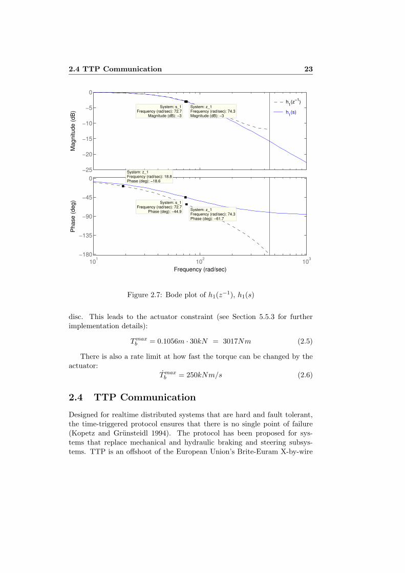
with Tb being the commanded brake torque to the actuator, aact = 0.6and bact = 0.4 which makes it equivalent to alow-pass filter. The transferfunction has a phase of −18.6 degrees at f = 3Hz and −61.7 degrees atf = 11.8Hz, cf. Figure 2.7. Sinusoidal experimental results (Ludemann2002) show that the EMB actuator has a phase of approximately −20 degreesat f = 3Hz and −60 degrees at f = 10Hz.
Figure 2.8 shows step responses of the actual EMB actuator and its twomodels, a first order (2.2) and a nonlinear (from Figure 2.5). The stepresponses of the first order and the non-linear models are similar (cf. Figure2.8), but the nonlinear model is better. The nonlinear brake model is onlyused for simulation. A corresponding continuous first order transfer functionfor equation (2.2) is
h1(s) =a
s + a(2.4)
where the parameter a = 72 rad/s is the bandwidth of the actuator.There are limitations on the clamping force that can be applied to the
brake pads by the actuator during braking. The (small) minimum force isto ensure that the brake pads are positioned close to the brake disk with noair-gap. The maximum force is what the actuator is capable of. Maximumbraking force with the EMB 4.0 actuator is 30 kN . The control input is theclamping force Fb that is related to the brake torque as Tb = kbFb, where theconstant kb depends on the friction between the brake pads and the brake
2.4 TTP Communication 23
Frequency (rad/sec)
Pha
se (d
eg)
Mag
nitu
de (d
B)
−25
−20
−15
−10
−5
0
System: z_1 Frequency (rad/sec): 74.3 Magnitude (dB): −3
System: s_1 Frequency (rad/sec): 72.7
Magnitude (dB): −3
101 102 103−180
−135
−90
−45
0
System: s_1 Frequency (rad/sec): 72.7
Phase (deg): −44.9 System: z_1 Frequency (rad/sec): 74.3 Phase (deg): −61.7
System: z_1 Frequency (rad/sec): 18.8 Phase (deg): −18.6
h1(s)
h1(z−1)
Figure 2.7: Bode plot of h1(z−1), h1(s)
disc. This leads to the actuator constraint (see Section 5.5.3 for furtherimplementation details):
Tmaxb = 0.1056m · 30kN = 3017Nm (2.5)
There is also a rate limit at how fast the torque can be changed by theactuator:
Tmaxb = 250kNm/s (2.6)
2.4 TTP Communication
Designed for realtime distributed systems that are hard and fault tolerant,the time-triggered protocol ensures that there is no single point of failure(Kopetz and Grunsteidl 1994). The protocol has been proposed for sys-tems that replace mechanical and hydraulic braking and steering subsys-tems. TTP is an offshoot of the European Union’s Brite-Euram X-by-wire

24 Test Vehicle
0.3 0.4 0.5 0.6 0.7 0.8 0.9 1 1.1 1.2 1.3
0
1000
2000
3000
4000
5000
6000
7000
8000
9000
10000
t [s]
F [N
]
Step responses
measurement nonlinear modellinear model
Figure 2.8: Verification of the brake models
project. In contrast to an event triggered system, a TTP system is built upby defining first the static message schedule (Hedenetz and Belschner 1998).Figure 2.9 shows the communication matrix of the brake-by-wire network inthe test vehicle. The lower part of Figure 2.9 shows the static synchronousTDMA (time division multiple access) schedule and its constraint whereeach subsystem has to send exactly once in a TDMA cycle. The messagesshown with ‘I’ are called I-Frames and are used for synchronization of lostmembers. I-Frames do not transmit information for the application layer,therefore they are not shown in the upper part of the matrix where thereceivers of the transmitted messages are located.
All communication between the BBWM, the PM and the ECU’s is basedon the fault tolerant TTP bus. The BBWM and the PM send their messagesin vice versa time slots. In this way short burst errors can be recovered. ABBWM slot has a length of about 0.88msec.New set points for the brakeforce can be sent every 7msec. The brake control ECU’s send their statusand the current brake force. These messages are not so time critical asthe transmission of the brake force set points. The brake ECU’s send theirmessages only once in a cluster cycle, which is 16 slots. In the availableslots, the brake ECU’s send I-Frames for the network management.

2.5 Brake-By-Wire-Manager and Power Manager 25
Brake1 X X X X X X X
Brake2 X X X X X X X
Brake3 X X X X X X X
Brake4 X X X X X X X
PM1 X X X X X X X X
PM2 X X X X X X X X
BBWM1 X X X X X X X
BBWM2 X X X X X X X
Brake1 I M
Brake2 M I
Brake3 I M
Brake4 M I
PM1 M M
PM2 M M
BBWM1 M M
BBWM2 M M
Slot 0 1 2 3 4 5 6 7 8 9 10 11 12 13 14 15
M Tx Message I Tx I-Frame X Rx Message
Transmit
Receive
TDMA cycle
Cluster cycle
Figure 2.9: Communication Matrix of the Brake-by-wire
2.5 Brake-By-Wire-Manager and Power Manager
The BBWM functionality is to read the values from the brake pedal sensors,the revolution counters of the wheels, the yaw-sensor, the acceleration sen-sors and to calculate from all these values the brake force (set points) for thefour brake actuators. The BBWM can manage higher assistance functionslike ABS, traction and driving dynamic control.
The ECU assumes all the system’s electrical, electronic and closed-loopcontrol functions. These include
• Power supply for all the system sensors
• Registration of operating conditions
• Data conversion (input/output drivers, A/D conversion)
• Data conditioning (calculation of manipulated variables using storedprogram maps)
• Data transmission (amplification and relay of signals to the systemactuators)

26 Test Vehicle
• CAN network linkage to other ECU’s.
The PM controls the battery charger, proceeds active power managementand monitors the status of the power supply. If the generator or one of theredundant power circuits should fail or the charge of the batteries is gettinglow, the PM generates a warning signal. Each of the four brake actuatorshave one brake ECU to control the electric motor of the brake actuator.
Figure 2.10 shows the schedule, which is periodically executed in theBBWM:
i. Pedal Signal Measurement - of the pedal signals from the three pedalsensors.
ii. Pedal Signal Plausibility Checks - from the three pedal signals, onevalid value is selected. This task is executed three times to detectfaults.
iii. Voter - a task votes over the result of the three plausibility check tasks.
iv. Brake Force Control - the brake forces for the four actuators are cal-culated. This task is also executed three times.
v. Voter - a task votes over the result of the three brake force controltasks.
vi. TTP Communication - the brake forces are send to the brakes via theTTP communication network.
vii. Diagnose - a diagnostic task.
viii. Diagnose Output - the diagnose values are transmitted to an externaldiagnosis device.
The Pedal Signal Plausibility Checks and the Brake Force Control areboth executed three times (due to being safety-related tasks) to discoverpossible faults. These two tasks are safety-related since they handle andmanipulate data variables, while the other tasks i.e. Pedal Signal Measure-ment, TTP-Communication, Diagnose and Diagnose Output, only handlemessages and are protected through cyclic redundancy checks (CRC).
This section is based on (Hedenetz and Belschner 1998).

2.5 Brake-By-Wire-Manager and Power Manager 27
Pedal Signal Measurement
Pedal Signal Plausibility Checks
Voter
Brake Force Control
Voter
TTP Communication
Diagnose
Diagnose Output
Timeslot 1 2 3 4 5 6 7 8
Figure 2.10: Local Task Schedule of the BBWM

28 Test Vehicle

Chapter 3
Wheel slip dynamics
This chapter will first discuss the slip dynamics which is used in the followingchapter for controller design. In Section 3.1, a mathematical model of thewheel slip dynamics is reviewed, see also (Burckhardt 1993; Freeman 1995;Drakunov, Ozguner, Dix, and Ashrafi 1995). Second part of this chapter willlook into friction models. The actual friction model used in this researchwas provided by DaimlerChrysler and due to its confidentiality, no descrip-tion can be provided. Therefore, a section is provided as an introduction tofriction modelling followed by a section on estimation of friction curves tobe used on experimental data later in this thesis, where a friction curve isproduced from each experiment. Finally, suspension dynamics are consid-ered as it might affect the controller performance since it is not included inthe controller design.
3.1 Wheel slip dynamics
The problem of wheel slip control is best explained by looking at a quartercar model as shown in Figure 3.1. The model consists of a single wheelattached to a mass m. As the wheel rotates, driven by the inertia of themass m in the direction of the velocity v, a tyre reaction force Fx is generatedby the friction between the tyre surface and the road surface. The tyrereaction force will generate a torque that results in a rolling motion of thewheel causing an angular velocity ω. A brake torque applied to the wheel willact against the spinning of the wheel causing a negative angular acceleration.

30 Wheel slip dynamics
wv
F m gz= ·
F -m vx= ·
Tb
•
Figure 3.1: Quarter car forces and torques.
The equations of motion of the quarter car are
mv = −Fx (3.1)
Jω = r Fx − Tb sign(ω) (3.2)
wherem mass of the quarter vehiclev longitudinal speed at which the vehicle travelsω angular speed of the wheelFz vertical forceFx tyre friction forceTb brake torquer wheel radiusJ wheel inertia
The tyre friction force Fx is given by
Fx = Fzµ(λ, µH , α) (3.3)
where the friction coefficient µ is a nonlinear function of
λ longitudinal tyre slipµH maximum friction coefficient between tyre and roadα slip angle of the wheel
The longitudinal slip is defined by
λ =v − ωr
v(3.4)
3.1 Wheel slip dynamics 31
0 0.2 0.4 0.6 0.8 10
0.2
0.4
0.6
0.8
1
λ
µ
µH
µG
λo
0 0.2 0.4 0.6 0.8 10
0.2
0.4
0.6
0.8
1
λ
µ
dry
wet
0 0.2 0.4 0.6 0.8 10
0.2
0.4
0.6
0.8
1
µ
λ
µH
=0.95
µH
=0.8
µH
=0.5
µH
=0.3
µH
=0.1
0 0.2 0.4 0.6 0.8 10
0.2
0.4
0.6
0.8
1
λ
µ
summer tyre
winter tyre
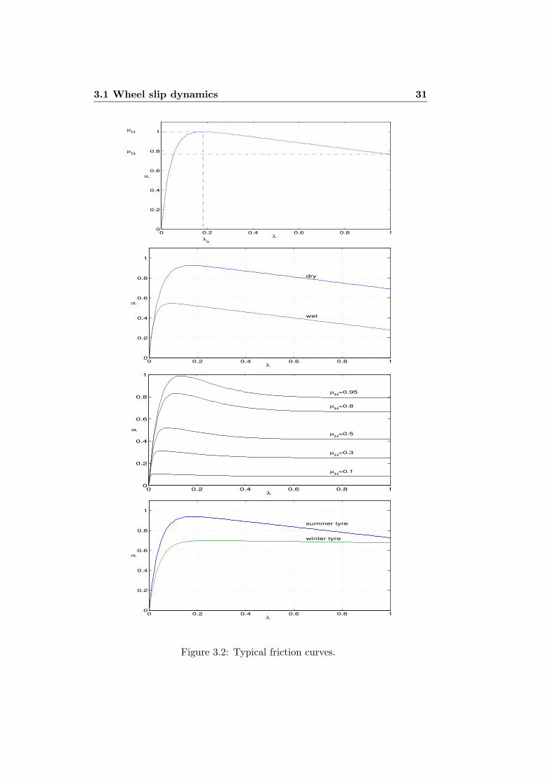
Figure 3.2: Typical friction curves.

32 Wheel slip dynamics
0 0.2 0.4 0.6 0.8 10
0.2
0.4
0.6
0.8
1
λ
µ
α = 0o
α = 10o
0 0.2 0.4 0.6 0.8 10
0.2
0.4
0.6
0.8
1
1.2
µ y
λ
α=1o
α=10o
Figure 3.3: Tyre side slip/friction curves. In top figure, µ = µx.
PSfrag replacements
α
vx
vy
v
Figure 3.4: Definition of wheel slip angle.

3.1 Wheel slip dynamics 33
Surface µH
Asphalt and concrete (dry) 0.8-0.9Concrete (wet) 0.8Asphalt (wet) 0.5-0.6Earth road (dry) 0.7Earth road (wet) 0.5-0.6Gravel 0.6Snow (hard packed) 0.3Ice 0.1
Table 3.1: Tyre/road friction peak
and describes the normalized difference between the vehicle speed v and thespeed of the wheel perimeter ωr. The slip value of λ = 0 characterizes thefree motion of the wheel where no friction force Fx is exerted. If the slipattains the value λ = 1, then the wheel is locked (ω = 0).
The friction coefficient µ can span over a very wide range, but is generallya differentiable function with respect to all arguments and has the propertiesµ(0, µH , α) = 0 and µ(λ, µH , α) > 0 for λ > 0. Its typical qualitativedependence on longitudinal slip λ is shown in Figure 3.2. The upper partshows how the friction coefficient µ increases with slip λ up to a value λ0,where it attains its maximum value µH . For higher slip values, the frictioncoefficient will decrease to a minimum µG where the wheel is locked and onlythe sliding friction will act on the wheel. The dependence of friction on theroad condition is shown in the two figures in the middle of Figure 3.2. Forwet or icy roads, the maximum friction µH is small and the right part of thecurve is flatter. The tyre friction curve will also depend on the brand of thetyre, as illustrated in the lower part of Figure 3.2. In particular, for wintertyres, the curve will cease to have a pronounced peak. Typical friction peakvalues (Burckhardt 1993; Gustafsson 1997; Hunter 1998; Canudas de Wit,Horowitz, and P.Tsiotras 1999) for different surface conditions are given inTable 3.1.
If the motion of the wheel is extended to two dimensions, then the lateralslip of the tyre must also be considered. The slip angle α is the angle betweenthe wheel bearing and the velocity vector of the vehicle, shown in Figure 3.4.In this case (Burckhardt 1993), the longitudinal slip
λx =vx − ωr
v(3.5)

34 Wheel slip dynamics
and the lateral slip
λy =ωr sin α
v= (1 − λx) sin α (3.6)
are distinguished as well as the longitudinal and lateral friction coefficients µx
and µy. vx is the wheel longitudinal speed in the wheel’s longitudinal direc-tion.
The upper part of Figure 3.3 shows the dependence of the friction coeffi-cient µx on the side slip angle α. The lateral friction is dramatically reducedas the longitudinal slip increases. The lateral friction µy depends greatly onthe side slip angle α and is shown in the lower part of Figure 3.3. Thelongitudinal force gets smaller as side slip angle is increased. This physicalphenomenon is the main motivation for ABS brakes, since avoiding highlongitudinal slip values will maintain high steerability and lateral stabilityof the vehicle during braking. Achieving this by manual control is difficultbecause the slip dynamics are fast and open loop unstable when operatingat wheel slip values to the right of any peak of the friction curve. Observethat a reasonable tradeoff between high longitudinal friction µx and lateralfriction µy is achieved under all road conditions for longitudinal slip λx closeto its peak value on the longitudinal slip curve. Hereafter, for simplificationpurposes unless otherwise stated, the side slip angle will be considered to bezero with µx = µ and vx = v.
Using (3.1)-(3.4), for v > 0 and ω ≥ 0, the wheel slip dynamics isobtained by calculating the time derivative of (3.4) with respect to time
λ =d
dt
(
1 − ωr
v
)
= − ωr
v+
ωr
v︸︷︷︸
1−λ
· vv
= −1
v
(1
m(1 − λ) +
r2
J
)
Fzµ(λ, µH , α) +1
v
r
JTb (3.7)
and
v = − 1
mFzµ(λ, µH , α) (3.8)
Notice that when v → 0, the open loop slip dynamics (from Tb to λ) becomesinfinitely fast with infinite high-frequency gain. Hence, the slip controllershould be switched off for small v. The following result shows that the

3.2 Friction modelling 35
interval [0, 1] is a positively invariant set for the wheel slip λ under thecondition that v > 0 and Tb ≥ 0 (i.e. there is braking and no traction):
Proposition 3.1 Consider the system (3.7)-(3.8) with Tb(t) ≥ 0 for allt ≥ 0. If v(0) > 0 and λ(0) ∈ [0, 1], then λ(t) ∈ [0, 1] and v(t) ≤ 0 for allt ≥ 0 where v(t) > 0.
Proof 3.1 Note that λ(t) is a continuous trajectory since v(t) > 0. Hence,the possible escape points are λ = 0 and λ = 1. Consider first λ = 0. Sinceµ(0, µH , α) = 0, it follows from (3.7) that λ = r
vJ Tb ≥ 0 due to Tb ≥ 0.Hence, λ(0) ≥ 0 implies λ(t) ≥ 0 for all t ≥ 0. Consider next λ = 1. Then,ω = 0 and from (3.2) it follows that ω ≥ 0 due to the discontinuity sign(ω)in (3.2). From (3.4), we conclude that λ = −rω/v ≤ 0, which impliesλ(t) ≤ 1 for all t ≥ 0. Finally, note that v ≤ 0 from (3.1) because Fx ≥ 0for λ ∈ [0, 1].
�
3.2 Friction modelling
The qualitative dependence of the tyre reaction forces on slip, type of tyreand road condition was explained in the previous section. Here, a back-ground to tyre friction modelling will be given.
Several tyre friction models describing the nonlinear behaviour are re-ported in the literature. There are static models as well as dynamic models,models which are constructed based on heuristical data as well as otherswhich have been derived from physical behaviour. The most reputed tyremodel is by (Bakker, Nyborg, and Pacejka 1987), and by (Pacejka and Sharp1991), also known as ”magic formula” and it is derived heuristically fromexperimental data. It provides the tyre/road coefficient of friction µ as afunction of the slip λ by using static maps. The ”magic formula” has beenshown to suitably match experimental data and is on the form:
Fx(λx) = D sin(C arctan(Bλx − E(Bλx − arctan(Bλx))))
The parameters, B − E, characterises the model and can be identified bycomparing experimental data as shown in (Bakker, Nyborg, and Pacejka1987). The model can also be used for modelling two other characteristics,the lateral force and the aligning torque. Effects due to either ply-steer orconicity effects are also taken into account (Pacejka and Sharp 1991).

36 Wheel slip dynamics
Surface conditions C1 C2 C3
Asphalt, dry 1.2801 23.99 0.52Asphalt, wet 0.857 33.822 0.347Concrete, dry 1.1973 25.168 0.5373Cobblestones, dry 1.3713 6.4565 0.6691Cobblestones, wet 0.4004 33.7080 0.1204Snow 0.1946 94.129 0.0646Ice 0.05 306.39 0
Table 3.2: Friction parameters
The expression in (Burckhardt 1993) is derived with similar methodologywhere µ is expressed as a function of the wheel slip, λ, and the vehiclevelocity, v. The vertical force on the tyre is assumed constant which gives
µx(λ, v) =[
C1
(
1 − e−C2λ)
− C3λ]
e−C4λv (3.9)
where the parameters are specified for different road surfaces, see Table 3.2(Kiencke and Nielsen 2000). The parameters in (3.9) denote the following:
C1 - maximum value of friction curveC2 - friction curve shapeC3 - friction curve difference between the maximum value
and the value at λ = 1C4 - wetness characteristic value and is in the range 0.02 − 0.04s/m.
(Daiß and Kiencke 1996) has simplified (Burckhardt 1993)’s model tomake it linear in the parameters (a and b) with the model
µ(λ) =kλ
aλ2 + bλ + 1
where k is the initial slope value (at λ = 0).
The dynamical tyre friction models can be formulated as a lumped ordistributed models, where a lumped friction model (Canudas de Wit, Olsson,Astrom, and Lischinsky 1995) assumes punctual tyre/road friction contactand a distributed model (Canudas de Wit, Horowitz, and P.Tsiotras 1999)assumes the existence of an area of contact between tyre/road. The lumped

3.2 Friction modelling 37
model is written on the form
g(vr) = µC + (µS − µC) e−|vr/vs|1/2
z = vr −σ0 |vr|g(vr)
z
Fx = (σ0z + σ1z + σ2vr)Fz
whereFx - the friction forceFz - normal forceσ0 - rubber longitudinal lumped stiffnessσ1 - rubber longitudinal lumped dampingσ2 - viscous relative dampingµC - normalized Coulomb frictionµS - normalized static friction, µC ≤ µS ∈ [0, 1]vS - Stribeck relative velocityvr - relative velocity = (rω − v)z - internal friction state
Apart from the nonlinear behaviour of the slip, the tyre friction dependson other uncertainties like road condition, tyre pressure, brand of tyre, tem-perature etc.
3.2.1 Estimation of friction curves
Fzf Fzr
MaX
Mg h
lrlf
Figure 3.5: Axle torque balance.
As the previous section has described some friction modelling strategiesand properties, it is of interest to be able to estimate a model of the surface

38 Wheel slip dynamics
conditions for different test scenarios based on the available experimentaldata.
Straight-line braking
The friction coefficient is defined as the ratio (3.3),
µ =Fx
Fz(3.10)
In order to estimate the friction coefficient µ, the values of Fx and Fz
are needed. This can be carried out using the method described in (Kienckeand Nielsen 2000). Equation (3.2) gives the longitudinal friction force Fx,which gives the friction value µ:
µ =Jω + Tb
Fzr(3.11)
The friction value can be found by using a torque balancing about thewheel axis (single wheel model). In order to find an expression for Fz, a fewassumptions can be made. The coupling between roll and pitch is neglected,thus the dependencies of the quarter vehicle forces on the longitudinal andlateral accelerations can be determined separately. By disregarding suspen-sion dynamics, the quarter vehicle forces are identical to the wheel verticalforces Fz.
The force due to longitudinal deceleration (Max) at the center of gravity(CoG), see Figure 3.5, causes a pitch torque which reduces the rear axle loadand increases the front axle load. Constructing the torque balance at therear axis contact point gives the front vertical force
lFzf = lrMg − hMax
⇓
Fzf =M(lrg − hax)
l(3.12)
where M is vehicle mass at CoG, ax is the longitudinal acceleration of CoG,h is the height of CoG and l = lf + lr . This gives the vertical force for asingle front wheel to be (Fz(f=front/r=rear,l=left/r=right))
Fzfl = Fzfr =M(lrg − hax)
2l(3.13)

3.2 Friction modelling 39
with the corresponding friction coefficient
µf =(Jω + Tb) 2l
M(lrg − hax)r(3.14)
Similarly, balancing the torque at the front axis contact point gives thevertical force (ground contact force) for a single rear wheel
Fzrl = Fzrr =M(lfg + hax)
2l(3.15)
with the corresponding friction coefficient
µr =(Jω + Tb) 2l
M(lfg + hax)r(3.16)
The same technique is applied to find the vertical force due to roll torques(assuming that the front and rear axles are decoupled). This gives the wheelforce, FZ , for the four wheel forces:
Fzfl =M(lrg − hax)
l
(1
2− hay
bfg
)
(3.17)
Fzfr =M(lrg − hax)
l
(1
2+
hay
bfg
)
(3.18)
Fzrl =M(lfg + hax)
l
(1
2− hay
brg
)
(3.19)
Fzrr =M(lfg + hax)
l
(1
2+
hay
brg
)
(3.20)
where ay (leftwards positive) is the lateral acceleration of CoG and bf andbr are the distances between wheels on the front and rear axles respectively.
Measurements needed for estimation of friction curve
A friction curve can then be plotted for each wheel from experiments, wherestationary wheel load is achieved, by post-calculating experimental data.This will yield friction curves (Section 6) which resemble what is shown inSection 3.1.
To obtain the friction value from equations (3.14,3.16,3.17-3.20), thewheel angular acceleration (ω), the brake torque (Tb), the longitudinal de-celeration (ax), lateral acceleration (ay) and the position of the center ofgravity are required. The brake torque, Tb, is derived from the measured

40 Wheel slip dynamics
clamping force.The wheel angular acceleration is calculated from the differ-ences between two consecutive samples of the wheel angular speed:
ω(n) =ω(n) − ω(n − 1)
Ts(3.21)
3.3 Suspension dynamics
A suspension system can be best studied as a dynamic system by lookingat the basic properties of the suspensions properties, i.e. the motions ofthe body and the axles. Due to the suspension dynamics, there may beresonance frequencies which will cause oscillations in the suspension system.Therefore, a wheel slip control design should, if possible, be tuned to avoidexciting the suspension system.
The inputs to the suspension system are the road displacement and thevertical force on the body, while the output is the vertical motion of the bodywhen a quarter car model is considered, as shown in Figure 3.6, where thesuspension can be seen to have stiffness and damping properties. The tyreis also represented with spring/damper, although the amount contributedby the viscoelastic damping can be neglected.
���
���� � � ��
� �
� ��
��
��
� � � �� ��
� � � � !
Figure 3.6: Quarter car model of suspension.
In Figure 3.6, x1 is the vehicle body displacement, x2 is the wheel dis-placement and hroad is the road profile (Gillespie 1992). Fz is the vertical

3.3 Suspension dynamics 41
mw = 55kg Wheel/suspension massmq = 395kg 1/4 of vehicle body mass (excluding wheels)ks = 24kN/m Suspension spring stiffnesskw = 200kN/m Tyre stiffnessds = 1350Ns/m Suspension damping constantdw = 120Ns/m Tyre damping constant
Table 3.3: Suspension parameters
force on suspension as described in Section 3.1: Fz vertical force from tyreto road surface, which includes a vertical force component acting on thevehicle body due to the pitch moment when the vehicle is braking. Otherparameters, typical values for a sporty sedan family car, are given in Table3.3 (Mastinu 1988; Dixon 1996; Kiencke and Nielsen 2000).
The torque balance between the pitch torque around the centre of gravitygives (roll dynamics together with the constant gravity force are neglected):
h (Fxf + Fxr) = lfFzf − lrFzr (3.22)
For illustration purposes let lf = lr, then (3.22) can be rewritten as
F bodyz =
h
lfFx (3.23)
where Fx = Fxf + Fxr, F bodyz = Fzf − Fzr and h is the height of CoG. The
horizontal distances from COG to the front and rear wheel axels are lf andlr respectively. This notation is also explained and used in Section 3.2.1 (seeFigure 3.5).
Using Newton’s Second Law, the vertical dynamics for a quarter vehiclecan be written as follows:
mqx1 = F bodyz − ds(x1 − x2) − ks(x1 − x2) (3.24)
mwx2 = ds(x1 − x2) + ks(x1 − x2) + dw(hroad − x2) + kw(hroad − x2)
(3.25)
Since the motion equations (3.24) and (3.25) represent a linear system,frequency domain analysis can be used by taking the Laplace transform ofthe above equations (all initial conditions are set to zero):
(mqs2 + dss + ks)X1(s) − (dss + ks)X2(s) = F body
z (s) (3.26)

42 Wheel slip dynamics
−(dss + ks)X1(s) + (mws2 + (ds + dw)s + (ks + kw))X2(s) =
(dws + kw)Hroad(s) (3.27)
which can be written on the form
A(s)
[X1(s)X2(s)
]
=
[
F bodyz (s)
(dws + kw) Hroad(s)
]
(3.28)
where
A(s) =
[mqs
2 + dss + ks − (dss + ks)− (dss + ks) mws2 + (ds + dw)s + (ks + kw)
]
(3.29)
Undamped resonance frequencies found by solving det(A(jω)) = 0 withds = dw = 0:
mqmwω4 − (mq (ks + kw) + ksmw) ω2 + kskw = 0 (3.30)
Equation (3.30) gives the undamped resonance frequencies fund1 = 0.6Hz
and fund2 = 10.2Hz. The fund
1 resonance is largely due to the movement ofthe vehicle body and the fund
2 resonance comprises mostly the movement ofthe wheel cf. Figure 3.7.
An analysis of a forced quarter vehicle model with damping and a har-monic input, is done by rewriting (3.28):
[X1(s)X2(s)
]
= A−1(s)
[
F bodyz (s)
(dws + kw) Hroad(s)
]
(3.31)
A−1(s) =1
∆(s)
[mws2 + (ds + dw)s + (ks + kw) dss + ks
dss + ks mqs2 + dss + ks
]
(3.32)where (∆(s) = det A(s))
∆(s) = mqmws4 + [mq (ds + dw) + dsmw] s3
+ [mq (ks + kw) + dsdw + ksmw] s2
+[dskw + ksdw]s + kskw (3.33)
Further, (3.31) can then be rewritten as

3.3 Suspension dynamics 43
[X1(s)X2(s)
]
=1
∆(s)A1(s)
[
F bodyz (s)
Hroad(s)
]
(3.34)
where elements of the A1(s) matrix are:
a1,1(s) = mws2 + (ds + dw)s + (ks + kw) (3.35)
a1,2(s) = dsdws2 + (dskw + dwks) s + kskw (3.36)
a2,1(s) = dss + ks (3.37)
a2,2(s) = mqdws3 + (mqkw + dsdw)s2 + (dskw + dwks) s + kskw (3.38)
Using (3.34), the transfer function for the vertical body acceleration
X1(s) with input F bodyz (s) becomes:
X1(s)
F bodyz (s)
=s2X1(s)
F bodyz (s)
(3.39)
⇓
G1(s) =X1(s)
F bodyz (s)
=mws4 + (ds + dw)s3 + (ks + kw)s2
∆(s)(3.40)
Similar, the transfer function for the vertical wheel acceleration X2(s)
with input F bodyz (s):
G2(s) =X2(s)
F bodyz (s)
=dss
3 + kss2
∆(s)(3.41)
Figure 3.7 shows the frequency responses for the vehicle body (3.40) andthe wheel (3.41). The vehicle body has a resonance frequency at f c
1 ≈ 1.3Hzand the wheel has a resonance frequency at fw
2 ≈ 10.1Hz.
Another way to view the dynamics is to consider the distance x1−x2, asthe deformation x2 − hroad is negligible. For the situation where the vehicleunder excitation by Hroad(s), with F body
z (s) = 0, the transfer function forthe chassis displacement becomes
X1(s)
Hroad(s)=
dsdws2 + (dskw + dwks) s + kskw
∆(s)(3.42)
and the transfer function for the vertical wheel displacement:

44 Wheel slip dynamics
Magnitude (abs)
Hz5 10 150
0.5
1
1.5
2
2.5
3
..X
2(s)
Fz(s)/m
q
..X
1(s)
Fz(s)/m
q System: G2 Frequency (Hz): 10.1 Magnitude (abs): 0.943
System: G2 Frequency (Hz): 1.26 Magnitude (abs): 0.328
System: G1 Frequency (Hz): 1.26 Magnitude (abs): 2.76
Figure 3.7: Frequency responses, G1(s) and G2(s), with Fz as input.
X2(s)
Hroad(s)=
mqdws3 + (mqkw + dsdw)s2 + (dskw + dwks) s + kskw
∆(s)(3.43)
The transfer function for the distance X1(s) − X2(s) where the vehicle
is under excitation by the Hroad(s) (and with F bodyz (s) = 0), is:
G3(s) =X2(s) − X1(s)
Hroad(s)=
mqdws3 + mqkws2
∆(s)(3.44)
Figure (3.8) shows the frequency response for (3.44), the vertical differ-ence between the chassis and the undercarriage contact points with road asinput. The resonance frequencies are f
xdiff
1 ≈ 1.3Hz and fxdiff
2 ≈ 9.6Hz.Similar methods and results are shown in (Gillespie 1992; Kiencke andNielsen 2000).
As shown above, the suspension dynamics has consequences for the wheelslip control design. Figure 3.9 shows how the suspension dynamics interactswith the ABS system through the loop in which the friction force appliedby the ABS controller causes a pitching moment, which again will affect thevertical force and back on the friction force. As a result of this suspension

3.3 Suspension dynamics 45
Magnitude (abs)
Hz0 5 10 150
0.5
1
1.5
2
2.5
X2(s)−X
1(s)
Hroad
(s)
System: G3 Frequency (Hz): 9.6 Magnitude (abs): 2.18
System: G3 Frequency (Hz): 1.26 Magnitude (abs): 2.5
Figure 3.8: Frequency response, G3(s), with road position as input.
analysis, the tuning of the wheel slip controller should take into account thesuspension dynamics and avoid the suspension resonance at fw
2 ≈ 10.1Hz.
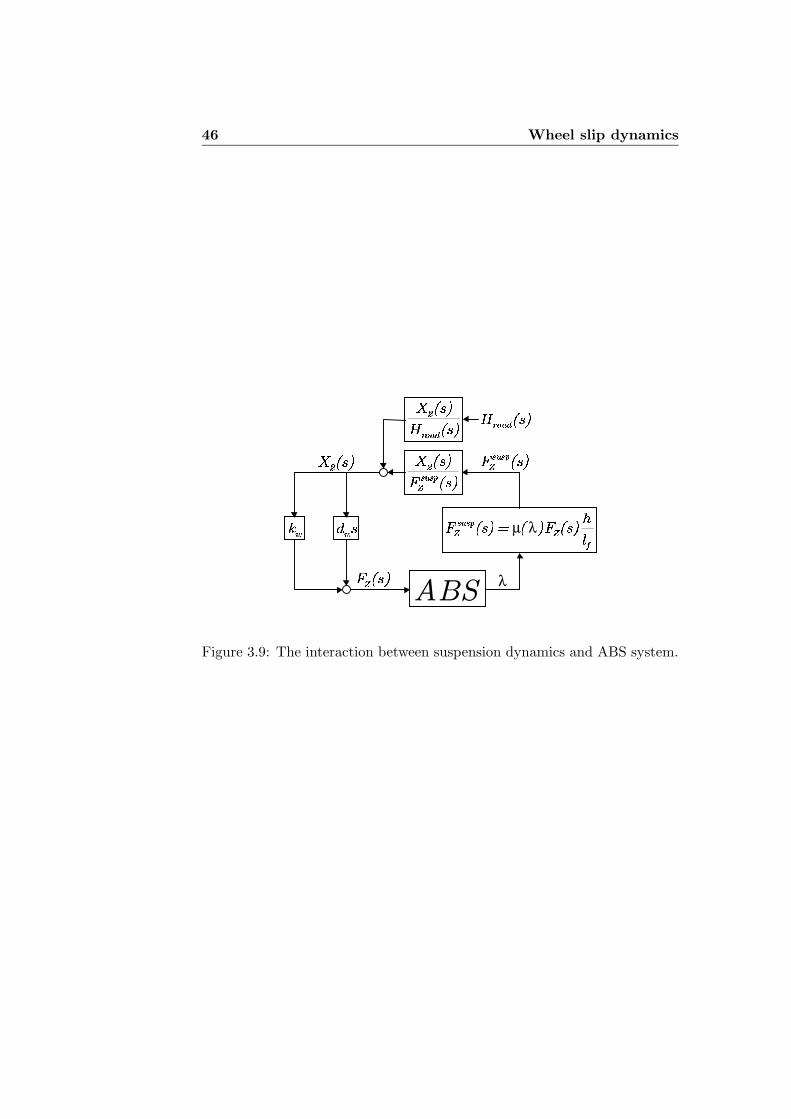
46 Wheel slip dynamics
"# $ % &')( * +,-( * +
./10
2354 6 7
8 9 8 :;<>= ? @
µ λA B A CD DFE
GH>I J K�LMINKOH5I J K P
QR S R TUV)W X YZ[W X Y
\]
ABS
^ _ ` abFc d e
λ
fg)h i j
Figure 3.9: The interaction between suspension dynamics and ABS system.
Chapter 4
Gain scheduled wheel slipcontrol
The wheel slip control problem is essentially to regulate the value of the lon-gitudinal slip λ to a given setpoint λ∗, which is either constant or commandedfrom a higher-level control system such as ESP. The controller must be ro-bust with respect to uncertainties in the tyre characteristic and the brakepads/discs, the variations in the road surface conditions, the load on thevehicle, etc. Integral action or adaptation must be incorporated to removesteady-state error due to model inaccuracies, in particular the unknownroad/tyre friction coefficient µH .
This chapter explains the linearized slip dynamics and the wheel slipcontrol design and analysis for i) system with just slip dynamics and nointegral action ii) with integral action and iii) with actuator dynamics.
4.1 Motivation for gain scheduling
The dynamics of the wheel and car body are given by (3.7) and (3.8) re-spectively. Due to large differences in inertia, the wheel dynamics and carbody dynamics will evolve on significantly different time scales. The speedv will change much more slowly than the wheel slip λ, and v is thereforea natural candidate for gain scheduling. Thus, for the control design, only(3.7) is considered and v is regarded as a slow time-varying parameter. Again scheduled control design requires a set of nominal linearized models fordesign.
Model-based nonlinear wheel slip control design shown in (Ludemann2002) depends strongly on knowing the friction coefficient and the friction

48 Gain scheduled wheel slip control
curve. The aim is to obtain (a robust) control design method which achievesrobustness by avoiding using the uncertain friction model in the design.
4.2 Linearized slip dynamics
Let (λ, Tb) be an equilibrium point for (3.7) defined by the nominal valuesα, Fz and µH
Tb =
(J
mr(1 − λ) + r
)
Fzµ(λ, µH , α) (4.1)
The speed-dependent nominal linearized slip dynamics are given by
λ =α1
v(λ − λ) +
β1
v(Tb − Tb) + h.o.t. (4.2)
where α1 and β1 are linearization constants given by
α1 = − Fz
(1
m(1 − λ) +
r2
J
)∂µ
∂λ(λ, µH , α) + Fz
1
mµ(λ, µH , α) (4.3)
β1 =r
J(4.4)
and ”h.o.t” denotes ”higher-order terms”. Notice that for nominal wheelslip values λ to the right of any peak of the friction curve, α1 > 0, suchthat the open-loop dynamics becomes open-loop unstable. For nominal slipvalues λ sufficiently to the left of any peak, α1 < 0, and the dynamics areopen-loop stable. Assuming arbitrary values of α, Fz and µH , the wheel slipdynamics (3.7) can be written in the form
x2 =φ(x2)
v+
β1
v(Tb − T ∗
b ) (4.5)
where x2 = λ−λ∗ and λ∗ is the desired slip (setpoint). Furthermore, define
φ(x2) = −(
1
m(1 − λ∗ − x2) +
r2
J
)
Fzµ(x2 + λ∗, µH , α) +r
JT ∗
b (4.6)
and
T ∗b =
(J
mr(1 − λ∗) + r
)
Fzµ(λ∗, µH , α) (4.7)
It can be seen that (4.5) has an equilibrium point given by x2 = 0, Tb = T ∗b
since φ(0) = 0, and the linearized slip model (4.2) with a perturbation termis written as follows
x2 =α1
vx2 +
β1
v(Tb − T ∗
b ) +εµ(x2)
v(4.8)

4.3 Wheel slip control design and analysis 49
where εµ(x2) = φ(x2) − α1x2. Eq. (4.8) will be used later on for controldesign and analysis.
4.3 Wheel slip control design and analysis
4.3.1 Without integral action
For simplicity, a design without integral action is studied first and wherethe infinite-horizon quadratic cost function is defined as:
J(x(t), u[t,∞)) =
∫ ∞
t(x2(τ)Q(v) + u2(τ)R)dτ (4.9)
with R > 0 and Q(v) ≥ 0 for all v > 0. Assuming v is constant (dueto the separation of time-scales) and neglecting the nonlinearity εµ(x), theoptimal control law (Anderson and Moore 1989) is uniquely given by thegain scheduled state feedback
u = −R−1 β1
vP (v)x = K(v)x, where K(v) = −R−1 β1
vP (v) (4.10)
The algebraic Riccati equation is
2P (v)α1
v−(
P (v)β1
v
)2
R−1 + Q(v) = 0 (4.11)
with the positive solution
P (v) =α1 +
(α2
1 + β21R−1Q(v)
)1/2
β21R−1
v = P′
(v)v (4.12)
Due to actuator constraints, the saturated control is defined as
u =
Tmaxb − T ∗
b , u > Tmaxb − T ∗
b
Tminb − T ∗
b , u < Tminb − T ∗
b
u, otherwise(4.13)
for some Tmaxb > Tmin
b ≥ 0. Furthermore, the error (note that both u and udepend on v and x) is defined as
εs(x, v) = β1(u − u) (4.14)
With the definition ε(x, v) = εs(x, v) + εµ(x), the closed loop dynamics canbe written as
x =
(α1
v+
β1K(v)
v
)
x +ε(x, v)
v(4.15)
It is easy to see that ε(0, v) = 0 for all v > 0.

50 Gain scheduled wheel slip control
Proposition 4.1 Consider the system (3.7) with controller (4.13), where
R > 0 and the smooth function Q satisfies Q(v) ≥ 0 and dQ(v)dv ≥ 0 for all
v > 0. Suppose for some δ ∈ (0, 1)
xε(x, v) ≤ (1 − δ)Q(v)
2P ′(v)x2 (4.16)
for all v > 0 and x ∈ [−λ∗, 1− λ∗]. Then, for all v(0) > 0 and λ(0) ∈ [0, 1],the equilibrium x = 0 is uniformly exponentially stable.
Proof 4.1 Let a Lyapunov function candidate be defined as
V (x) = x2P (v) (4.17)
Along trajectories of (4.15), one has
V =d
dtV (x) = x2
(dP (v)
dv
dv
dt
)
+ 2xxP (v) (4.18)
Substituting for (4.8), (4.10) and (4.11) in (4.18) gives
V = x2
(
P′
(v) + vdP
′(v)
dv
)
v + 2ε(x, v)P′
(v)x − x2Q(v) (4.19)
Note that P′
(v) ≥ 0 and dP′(v)
dv ≥ 0 for all v > 0. It follows from Proposition3.1 that
V ≤ 2ε(x, v)P′
(v)x − x2Q(v) ≤ −δQ(v)x2 (4.20)
and the equilibrium is uniformly exponentially stable by Corollary 3.4, in(Khalil 1996), since V (x) and the right hand side in (4.20) are upper andlower bounded by a positive definite quadratic functions in x for all v ≥ vmin.The region of attraction follows from Proposition 3.1 since [0, 1] is positivelyinvariant for λ.
�
Essentially, (4.16) requires that the error weight Q(v) must be chosensufficiently large, which means that the gain K(v) must be sufficiently largein order to stabilize the system. Note that the system is open loop unstablewhen operating in a region where the friction curve has negative slope ∂µ
∂λ(in this case α1 > 0). The controller is gain scheduled since K depends on
v. From a practical point of view, it makes sense to choose dQ(v)dv > 0 since
this leads to dK(v)dv > 0. Hence, the gain is reduced as v → 0 and one avoids

4.3 Wheel slip control design and analysis 51
instability due to unmodelled dynamics that typically become dominant asv → 0.
The above analysis shows that the heuristics of local linearization andgain scheduling do not lead to instability when Q(v) is chosen sufficientlylarge. Unfortunately, it is not possible to implement this controller withoutsignificant loss of performance since the steady state brake torque T ∗
b isunknown; recall that Tb = T ∗
b + u and T ∗b depends on µH which is highly
uncertain and time-varying. Hence, all practical wheel slip controllers needsome form of integral action or adaptation. Thus, the design and analysisis extended with integral action without further discussion.
4.3.2 With integral action
Let the system dynamics (4.8) be augmented with a slip error integratorx1 = λ − λ∗ = x2 such that
(x1
x2
)
= A(v)
(x1
x2
)
+ B(v) (u − T ∗b ) + W (v)εµ(x2) (4.21)
where
A(v) =
(0 10 α1
v
)
, B(v) =
(0β1
v
)
, W (v) =
(01v
)
(4.22)
The steady-state brake torque T ∗b depends on road and tyre properties
such as µH and must therefore be assumed unknown. Hence, the controlinput is defined as u = Tb, and the equilibrium point is
x∗ =
(x∗
1
0
)
, u∗ = T ∗b (4.23)
where the value x∗1 depends on the controller due to the integral action. This
leads to
x = A(v) (x − x∗) + B(v) (u − u∗) + W (v)εµ(x2) (4.24)
Next, the quadratic cost function for the purpose of local LQ designbased on the nominal part of (4.24), is defined as follows:
J(x(t), u[t,∞)) =
∫ ∞
t((x(τ) − x∗)T Q(v) (x(τ) − x∗)
+ (u(τ) − u∗)T R (u(τ) − u∗))dτ (4.25)

52 Gain scheduled wheel slip control
Assuming constant v, the optimal control law (Anderson and Moore1989) is given by
u = K(v)x (4.26)
where the gain matrix is K(v) = −R−1BT (v)P (v). The unknowns x∗ andu∗ are neglected, which will be accounted for due to the integral action.The symmetric matrix P (v) > 0 is defined by the solution to the associatedalgebraic Riccati equation:
P (v)A(v) + AT (v)P (v) − 2P (v)B(v)R−1BT (v)P (v) = −Q(v) (4.27)
The elements of the matrix equation (4.27) are(
β1
v
)2 P 21,2(v)
R= Q1,1(v) (4.28)
P1,1(v) + P1,2(v)
(
α1
v−(
β1
v
)2 P2,2(v)
R
)
= 0 (4.29)
2P1,2(v) + P2,2(v)
(
2α1
v−(
β1
v
)2 P2,2(v)
R
)
= −Q2,2(v) (4.30)
This gives the following solution with P (v) > 0:
P1,1(v) =
(
α21 + β2
1R−1
(
Q2,2(v) +2(Q1,1(v)R)1/2
β1v
))1/2
(Q1,1(v)R)−1/2 β1
(4.31)
P1,2(v) =v
β1(Q1,1(v)R)1/2 (4.32)
P2,2(v) =
α1 +
(
α21 + β2
1R−1
(
Q2,2(v) +2(Q1,1(v)R)1/2
β1v
))1/2
β21R−1
v (4.33)
and the gains
K1(v) = −(Q1,1(v)R−1
)1/2(4.34)
K2(v) = −α1 +
(
α21 + β2
1R−1
(
Q2,2(v) +2(Q1,1(v)R)1/2
β1v
))1/2
β1(4.35)
Setting x∗1 = T ∗
b /K1(v) gives the closed loop error dynamics
˙x = (A(v) + B(v)K(v)) x + W (v)εµ(x2) (4.36)
with the controller error x = x − x∗.

4.3 Wheel slip control design and analysis 53
Proposition 4.2 Consider the system (3.7) with controller defined by (4.26)and (4.34)-(4.35). Assume R > 0 and the smooth matrix-valued function
Q satisfies Q1,2(v) = Q2,1(v) = 0, Q1,1(v) > 0, Q2,2(v) > 0,dQ1,1(v)
dv ≥ 0,dQ2,2(v)
dv ≥ 0 for all v ≥ vmin > 0. Moreover, suppose Tb(t) ≥ 0 for all t ≥ 0and
D(v) = P′
1,1(v)P′
2,2(v) − P′
1,2(v)P′
2,1(v) > 0 (4.37)
Q1,1(v)(1 − δ) >P2,1(v)C
v(4.38)
Q2,2(v)x22(1 − δ) >
(
2
vεµ(x2)P2,2(v)x2 +
P2,1(v)ε2µ(x2)
vC
)
(4.39)
are satisfied for all v ≥ vmin > 0, x2 ∈ [−λ∗, 1 − λ∗] and some C > 0 andδ ∈ (0, 1). Then, the equilibrium x = 0 is uniformly exponentially stable.
Proof 4.2 Let a Lyapunov function candidate be
V (x) = xT P (v)x (4.40)
Its time-derivative along trajectories of (4.36)
V =d
dtV (x(t)) = xT
(dP (v)
dvv
)
x + ˙xT Px + xT P ˙x (4.41)
is found by substituting for (4.24), (4.26) and (4.27) in (4.41):
V = xT dP (v)
dvvx + εµ(x2)(W
T (v)P (v)x + xT P (v)W (v))− xT Q(v)x (4.42)
From Proposition 3.1, it is clear that v ≤ 0 since Tb ≥ 0. Thus, the non-
positivity of xT(
dP (v)dv v
)
x requires P ′(v) = dP (v)dv > 0 for all v > 0. For
P′
(v) to be positive definite, it is sufficient that P′
1,1(v) > 0 since D(v) > 0.
Note that since Q1,1(v), Q2,2(v), β1 > 0, it follows immediately that P′
1,1(v) >0. Then, (4.42) becomes:
V ≤ εµ(x2)(WT P (v)x + xT P (v)W (v)) − xT Q(v)x
= −Q1,1(v)x21 − Q2,2(v)x2
2 +2
vεµ(x2)(P2,2(v)x2 + P2,1(v)x1) (4.43)
To obtain all x1-terms in (4.43) in a quadratic form, Young’s inequality2ab ≤ a2/C + Cb2 is applied. Hence,
V ≤ −Q1,1(v)x21 +
P2,1(v)
vx2
1C − Q2,2(v)x22
+2
vεµ(x2)P2,2(v)x2 +
P2,1(v)
v
ε2µ(x2)
C(4.44)

54 Gain scheduled wheel slip control
Due to (4.38) and (4.39) it follows that
V ≤ −δQ1,1(v)x21 − δQ2,2(v)x2
2 (4.45)
and one concludes that the equilibrium is uniformly exponentially stable byCorollary 3.4, in (Khalil 1996), since V (x) and the right hand side in (4.38)are upper and lower bounded by a positive definite quadratic functions in xfor all v ≥ vmin.
�
Inequality (4.38) states that the error weight Q1,1(v) must be sufficientlylarge, leading to a sufficiently large controller gain. In this inequality, P2,1(v)depends on Q1,1(v), but it is evident that P2,1(v) increases with
√Q1,1(v)
such that (4.38) will indeed hold for a sufficiently large Q1,1(v), except whenv → 0.
Inequality (4.39) states that the error weight Q2,2(v) must also be suf-ficiently large, leading to a sufficiently high gain to stabilize the system.Note that P2,2(v) increases with
√Q2,2(v) such that this is also possible,
except for v → 0. In (4.39), Q2,2(v) |x2| is essentially chosen to dominatethe perturbation ε(x2). Inequality (4.39) must be checked with respect tothe perturbations εµ that are generated by all possible friction curves µ(·)to ensure robust stability.
Inequality (4.37) can be seen to be non-restrictive since it will always besatisfied for α1 close to zero, see Appendix B. This corresponds to gener-ating the nominal model by linearizing near the peak of the friction curve.Experience shows that high performance is indeed achieved this way. Forα1 = 0, no information on the friction curves is actually utilized in thecontrol design.
The constant C > 0 should be chosen to minimize conservativeness.However, the choice Q1,2(v) = Q2,1(v) = 0 and taking P (v) from the solu-tions of the Riccati equation are possibly conservative.
The controller gain K(v) depends on the speed (gain scheduling). From a
practical point of view, a useful gain schedule is achieved by lettingdQ1,1(v)
dv >
0 anddQ2,2(v)
dv > 0, as this reduces the gain as v → 0. As mentioned earlier,this is necessary to avoid instability due to the unmodelled dynamics sincethese tend to dominate as v → 0.
An important aspect is the initialization of the integrator state x1. Notethat x1 is a controller state that can be initialized arbitrarily, while x∗
1 isunknown since it depends on the road/tyre friction coefficient µH . Hence, anintelligent initialization of x1(0) based on any a priori information on µH and

4.3 Wheel slip control design and analysis 55
possibly on the known x2(0), may significantly improve the transient per-formance after the controller is activated (Johansen, Kalkkuhl, Ludemann,and Petersen 2001).
An idealized design example
Consider a design example with the following parameters m = 450 kg, Fz =4414 N , r = 0.32 m, J = 1.0 kg m2 and the friction model in the thirdpart of Figure 3.2. Assuming λ∗ = 0.14 and the nominal friction parametersµ∗
H = 0.8 and α∗ = 0, this give α1 = 10.2 and β1 = 0.32. Choose R = 1 andQ(v) = Qv3/2 with Q1,1 = 6 · 109 and Q2,2 = 40 · 106. Note the scaling dueto the different magnitudes of Tb and λ. The choice for Q(v) leads to a gainschedule with reduced gain as v → 0, which is useful to avoid instability dueto unmodelled dynamics as v → 0.
Figures 4.1 and 4.2 show that the robust stability requirement (4.39) issatisfied for all x2 ∈ [−λ∗, 1−λ∗] for all the friction curves in the third figureof Figure 3.2. Although curves are shown only for v = 1 m/s and v = 32m/s, (4.37) has been verified to be fulfilled for intermediate values of v. Thecontrol design also satisfies the stability requirements (4.38) and (4.37), andgives robust uniform exponential stability of the equilibrium.
4.3.3 With actuator dynamics
Next, a gain scheduled LQ approach is described for a wheel slip control de-sign where the actuator dynamics are taken into account, the integral actionis included and the rate of the clamping force is used as the control input.The latter is introduced partly to simplify the handling of rate constraints inthe implementation and partly to get velocity-based gain scheduled control,the benefits of which are reported in (Kaminer, Pascoal, Khargonekar, andColeman 1995; Leith and Leithead 1996). The dynamics of the augmentedsystem are given by the following equations
x1 = x2 (4.46)
x2 =α1
vx2 +
β1
v(x3 − T ∗
b ) +1
vεµ(x2) (4.47)
x3 = −a(x3 − T ∗b ) + a(x4 − T ∗
b ) (4.48)
x4 = u (4.49)
The state x1 is the integrated slip error (giving integral action), x2 is the sliperror, x3 is the clamping torque produced by the actuator, x4 is the clamping

56 Gain scheduled wheel slip control
torque commanded to the actuator and u is the commanded rate of changeof the clamping torque. The parameter a = 72 rad/s is the bandwidth ofthe actuator, see Section 2.3.2. With
A(v) =
0 1 0 0
0 α1v
β1
v 00 0 −a a0 0 0 0
B =
0001
, W (v) =
01v00
the system can be written as the following linear parameter-varying (LPV)system with a perturbation:
x = A(v)(x − x0) + Bu + W (v)εµ(x2) (4.50)
where x0 = (0, 0, T ∗b , T ∗
b ). Assuming a fixed v, the gain scheduled LQ con-troller (Anderson and Moore 1989) is given in the form
u = −K(v)x (4.51)
where the matrix K(v) is computed by solving the following standard linearquadratic optimal control problem
J(u, x(t), v) =
∫ ∞
t
(xT (τ)Q(v)x(τ) + Ru2(τ)
)dτ (4.52)
Note that x is known while x0 is unknown as T ∗b depends on the tyre
parameters, vertical load, wheel slip angle, road friction, etc.
An idealized design example
The design parameters given in Section 4.3.2 are used with the followingmodifications. For the control design, Q1,1 = 8 · 106 and all other elementsof Q in Q(v) = Qv3/2 are set to zero. The choice for Q(v) leads to again schedule with reduced gain as v → 0, see Figure 4.3 (for presentationpurposes K1 has been reduced by a factor of 10 and K3 and K4 have beenincreased by a factor of 1000).
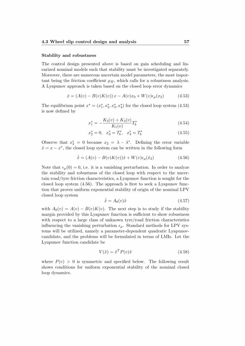
4.3 Wheel slip control design and analysis 57
Stability and robustness
The control design presented above is based on gain scheduling and lin-earized nominal models such that stability must be investigated separately.Moreover, there are numerous uncertain model parameters, the most impor-tant being the friction coefficient µH , which calls for a robustness analysis.A Lyapunov approach is taken based on the closed loop error dynamics
x = (A(v) − B(v)K(v)) x − A(v)x0 + W (v)εµ(x2) (4.53)
The equilibrium point x∗ = (x∗1, x
∗2, x
∗3, x
∗4) for the closed loop system (4.53)
is now defined by
x∗1 = −K3(v) + K4(v)
K1(v)T ∗
b (4.54)
x∗2 = 0, x∗
3 = T ∗b , x∗
4 = T ∗b (4.55)
Observe that x∗2 = 0 because x2 = λ − λ∗. Defining the error variable
x = x − x∗, the closed loop system can be written in the following form
˙x = (A(v) − B(v)K(v))x + W (v)εµ(x2) (4.56)
Note that εµ(0) = 0, i.e. it is a vanishing perturbation. In order to analyzethe stability and robustness of the closed loop with respect to the uncer-tain road/tyre friction characteristics, a Lyapunov function is sought for theclosed loop system (4.56). The approach is first to seek a Lyapunov func-tion that proves uniform exponential stability of origin of the nominal LPVclosed loop system
˙x = A0(v)x (4.57)
with A0(v) = A(v) − B(v)K(v). The next step is to study if the stabilitymargin provided by this Lyapunov function is sufficient to show robustnesswith respect to a large class of unknown tyre/road friction characteristicsinfluencing the vanishing perturbation εµ. Standard methods for LPV sys-tems will be utilized, namely a parameter-dependent quadratic Lyapunov-candidate, and the problems will be formulated in terms of LMIs. Let theLyapunov function candidate be
V (x) = xT P (v)x (4.58)
where P (v) > 0 is symmetric and specified below. The following resultshows conditions for uniform exponential stability of the nominal closedloop dynamics.

58 Gain scheduled wheel slip control
Proposition 4.3 Assume there exist a constant γ > 0 and a smooth func-tion P (v) that satisfies for all vmax ≥ v ≥ vmin > 0
P (v) > 0 (4.59)
dP
dv(v) ≥ 0 (4.60)
P (v)A0(v) + AT0 (v)P (v) + γP (v) ≤ 0 (4.61)
Then, the origin is a uniformly exponentially stable equilibrium for all trajec-tories of the nominal closed loop system (4.57) that satisfies −λ∗ ≤ x2(0) ≤1 − λ∗, x3(t) ≥ 0, x4(t) ≥ 0 and vmax ≥ v(t) ≥ vmin for all t ≥ 0.
Proof 4.3 V is a suitable Lyapunov function candidate since (4.59) ensuresthat it is positive definite with upper and lower bounds. Along trajectoriesof the nominal closed loop (4.57), the time-derivative of V is
V = xT (P (v)A0(v) + A0(v)T P (v))x + xT dP (v)
dvxv (4.62)
It is known from Proposition 3.1 that v ≤ 0 during braking such that(4.60) ensures that the last term in (4.62) is not positive. Hence, (4.61)implies that
V ≤ −γxT P (v)x = −γV (4.63)
It is then a standard result (Khalil 1996) that the origin is uniformly expo-nentially stable, i.e. x(t) tends to zero exponentially with rate bounded byγ/2.
�
In order to transform these conditions to standard LMI conditions, in-troduce a smooth parameterization of P (v) similar to (Gahinet, Apkarian,and Chilali 1996) and discretize a suitable interval for the parameter v:
P (v) = P0 + P1v1/2 + P2v + P3v
3/2 (4.64)
with symmetric 4 × 4 matrices P0, P1, P2 and P3. The terms dependingon v are motivated by the explicit expressions for P (v) in Section 4.3.2.Of course, in this case, a more complex parameterization may lead to aless conservative Lyapunov function so that it may prove a larger stabilitymargin. Conditions (4.59) - (4.60) are now given by
P (v) = P0 + P1v1/2 + P2v + P3v
3/2 > 0 (4.65)
dP
dv(v) =
P1
2v1/2+ P2 +
3
2P3v
1/2 ≥ 0 (4.66)
P (v)A0(v) + AT0 (v)P (v) + γP (v) ≤ 0 (4.67)

4.3 Wheel slip control design and analysis 59
Inequalities (4.65), (4.66) and (4.67) now define a standard LMI prob-lem (Boyd, Balakrishnan, Feron, and Ghaoui 1993) with the objective ofmaximizing the scalar variable γ > 0, where the LMI conditions are im-posed at a finite number of values v. A gridding approach is chosen be-cause the parameterization of P (v) is not convex. 12 values in the interval0.75m/s ≤ v ≤ 33m/s have been chosen. This leads to a solution of theLMI conditions (4.65) - (4.67) with γ = 26.9. It follows that the given de-sign makes the equilibrium point x = 0 locally exponentially stable whenthe setpoint is chosen λ∗ = 0.14, even in the presence of uncertainty in thefriction curve. The amount of uncertainty may, however, restrict the regionof attraction.
Given the γ > 0 and matrices P0, P1, P2, P3 that solve the above men-tioned LMI-problem, the Lyapunov function candidate may be examinedto show that it proves a stability margin to account for the uncertainty inεµ. Along the trajectories of the perturbed closed loop (4.56), the time-derivative of the Lyapunov function V for the nominal closed loop satisfies
V ≤ −γxT P (v)x + 2xT P (v)W (v)εµ(x2) (4.68)
In Figure 4.4, three figures are shown for V ; for v = 0.75, 8.5 and 24 m/srespectively. In the top figure, the side slip angle is α = 15 degrees andzero in the other two figures. In each figure, three curves are shown forµH(= 0.1, 0.5, 0.9). x1, x3 and x4 are set to their respective equilibriumvalues. Figure 4.4 shows that the robust stability requirement (4.68) issatisfied for all x2 ∈ [−λ∗, 1 − λ∗] for the selected friction curves. Althoughcurves are shown only for v = 0.75, 8.5 and 24 m/s, it has been verifiedthat (4.68) is fulfilled for intermediate values of v, λ and α. Unfortunately,this approach does not allow a rigorous conclusion, except local stability,since the Lyapunov-function candidate at hand appears to be conservativewhen x1, x3 and x4 are taken sufficient far from their equilibrium values.However, the analysis indicates the following observations that agree wellwith the experience from simulations and experiments:
• The robustness margins are most difficult to fulfill at low speeds (lessthan say 5 m/s), high µH and high α. This is as expected, since theuncertainty scales with 1/v and at high µH and α, the slip dynamicshave the highest degree of open loop instability.
• Largest robustness margins are achieved by placing the setpoint to theright of the friction curve peak. On the other hand, maximum frictionis achieved at the peak value and maximum steerability suggests that

60 Gain scheduled wheel slip control
the slip is as low as possible. In general, the slip value where the peakvalue is attained, is reduced as µH is reduced. Therefore, a reasonablecompromise is to let the setpoint be close to the peak value and dependon an estimate of µH .
• A higher robustness margin and stronger theoretical robustness resultscould be achieved by choosing larger values in the Q(v)-matrix, suchthat the feedback gain is increased. However, due to other unmodelledphenomena such as tyre dynamics, computer system communicationdelay and suspension dynamics, this is not possible in a practical de-sign.
4.4 Discussion
In this chapter, three theoretical results on wheel slip control design andanalysis are presented. A design analysis for a first order system containingonly wheel slip dynamics is shown. But, this controller design is cannot beimplemented without a significant loss of performance since the steady-statebrake torque is unknown. By incorporating integral action, steady-state er-rors due to model inaccuracies can be handled, it is shown to give uniformexponential stability. The actuator constraints are not considered in orderto present the stability results in a comprehensible way as the problem oth-erwise becomes too complex to analyze. To extend the model even furtherto achieve the best possible approximation to the test vehicle, actuator dy-namics and an integrator on the control input are included. Stability androbustness for variations in λ, µH , v and α are shown. But, for x1, x3 andx4 taken sufficient far from their equilibria the analysis is non-conclusive.
None of the controller designs and analysis shown in this chapter arein discrete time and they don’t incorporate saturation control. Still, theyprovide a starting point for the practical design and implementation usingthe LQRC method, as described in Chapter 5.

4.4 Discussion 61
0 0.1 0.2 0.3 0.4 0.5 0.6 0.7 0.8 0.9 1−1
−0.5
0
0.5
1
1.5
2
2.5
3x 10⁷
λx (longitudinal slip)
Left hand side
Right hand sides
0.11 0.12 0.13 0.14 0.15 0.16 0.17 0.18
−3
−2
−1
0
1
2
3
4
5
x 104
λx (longitudinal slip)
Left hand side
Right hand sides
Figure 4.1: Illustration of the robust stability requirement, i.e. the left andright hand sides of equation (4.39) for v = 1m/s. The bottom plot showsan expanded view.

62 Gain scheduled wheel slip control
0 0.1 0.2 0.3 0.4 0.5 0.6 0.7 0.8 0.9 1−1
−0.5
0
0.5
1
1.5
2
2.5
3x 10⁷
λx (longitudinal slip)
Left hand side
Right hand sides
Figure 4.2: Illustration of the robust stability requirement, i.e. the left andright hand sides of equation (4.39) for v = 32 m/s.
0 5 10 15 20 25 30 350
0.5
1
1.5
2
2.5
3
3.5
K1/10
K2
K3*1000
K4*1000
Speed v[m/s]
Figure 4.3: Gain K(v), as a function of v.

4.4 Discussion 63
0 0.1 0.2 0.3 0.4 0.5 0.6 0.7−15
−10
−5
0
µH=0.1
µH=0.5
µH=0.9
λ
dV/dt, v=0.75m/s and α=15o
0 0.1 0.2 0.3 0.4 0.5 0.6 0.7 0.8−9
−8
−7
−6
−5
−4
−3
−2
−1
0x 10
4
µH=0.1
µH=0.5
µH=0.9
λ
dV/dt, v=8.5m/s and α=0o
0 0.1 0.2 0.3 0.4 0.5 0.6 0.7 0.8−5
−4.5
−4
−3.5
−3
−2.5
−2
−1.5
−1
−0.5
0x 10
5
µH=0.1
µH=0.5
µH=0.9
λ
dV/dt, v=24m/s and α=0o
Figure 4.4: Time derivative of V .

64 Gain scheduled wheel slip control

Chapter 5
Implementation, redesignand tuning
An insight into the controller structure and states, and the ABS supervi-sory logic is given first to show the framework under which the controller wasimplemented. A brief description of the controller design method, LQRC,and how the system is specified for LQRC design are then given. The dis-crete time wheel slip control design and tuning shown in this chapter forimplementation use the control design parameters from the control designand analysis developed in Chapter 4 in addition to the actuator constraints.Note that the stability analysis developed in Chapter 4 is based on a gainscheduled LQG design to simplify the analysis and to obtain comprehensibleresults. However, experiments showed that the actuator rate constraints didnot have a significant impact on the experimental results. Then an analysisand a discussion are given on the choice of slip setpoint as the commu-nications delay and actuator dynamics impose limitations. Two methodsimproving the initial transient response, controller initialization and off-equilibrium scheduling on slip are then described. Towards the end of thischapter, a description of the implementation of an anti-windup mechanismis provided.
5.1 Controller structure
The overall structure of the controller that has been implemented in thevehicle is shown in Figure 5.1. It consists of the slip controller (LQRC),the extended Kalman filter (EKF) and the vehicle equipped with electrome-chanical brakes operating on unknown road surfaces. The shaded boxes

66 Implementation, redesign and tuning
represent the controller and related elements implemented in software. Thenon-shaded boxes represents the physical system. The online estimated vari-ables from the EKF (based on a nonlinear vehicle model) are:
• Tyre/road slip (λ)
• Vehicle velocity (v)
• Maxium friction coefficient (µH - not used for the LQRC design)
The measurements fed to the EKF are the four wheel speeds, the steer-ing wheel angle, the longitudinal and lateral accelerations. In general, it canbe said that the estimation error by the EKF leads to a loss in controllerperformance. For controller design, these variables are assumed as measure-ments and therefore, the dynamics of the estimator is not included in thedesign.
The brake-by-wire software is written in C and provides an interface forthe wheel slip controller. The interface gives access to the sensor signalsand reads the command signals for the brakes provided by the wheel slipcontroller. The wheel slip controller runs at a sampling period (Ts) of 7msecand with a delay of two time steps between the processing of a new controlsignal and until the sensor output has been received, see Figure 2.9 and 5.5.
Gain Schedule
LQRC ActuatorCar
Dynamics
ExtendedKalman
Filter
Slip
TorqueTorqueCmd.
Speed over ground
Figure 5.1: Wheel slip control - block diagram.
5.2 ABS supervisory logic
As a safety device, the ABS will only be activated when the driver commandsa brake force resulting in higher slips than the setpoint of the controller, typ-ical in critical or emergency situations. The maximal applied brake force islimited to the driver’s commanded brake force. For safety reasons, the slip

5.3 Controller states 67
controller is only allowed to lower the brake force in order to prevent thewheel from locking. When the commanded brake force by the driver is low-ered (by the brake pedal), the brake force should be decreased accordingly.
Figure 5.2 shows the on/off switching of the overall controller. An oper-ation state f is achieved only when the controller is switched on manually(S), the gear g is set to forward (not reverse) and the reference speed vr ofthe vehicle is higher than the minimum speed. Notice that the controller isswitched off when the velocity drops below a minimum speed (vmin = 1m/s).
PSfrag replacements
on off
f = 1 f = 0
init
(vr < vmin) ∨ S ∨ g
(vr ≥ vmin) ∧ S ∧ g
(vr ≥ vmin) ∧ S ∧ g (vr < vmin) ∨ S ∨ g
Figure 5.2: On/Off automaton
5.3 Controller states
Figure 5.3 shows the mode-switching automaton with three states. Thecontroller remains in manual mode when f is off. The automaton enters theautomatic state when f is on and the driver requests a brake force Fd thatis higher than minimal brake force Fmin, i.e. braking. If the brake pedal isreleased and f is off, the controller state is switched to manual state. If thebrake pedal is not released and f is off, the controller state is switches tobumpless transfer. Normally, when ABS is activated, the brake demandedby the driver is higher than the brake torque applied by the controller.Therefore, to avoid a jerky transfer from the automatic state to the manualstate with full brake force applied, a bumpless transfer is implemented. Inthe bumpless transfer state, the gradient of the brake force is limited untilthe output of the rate limiter has reached the desired clamping force Fd andthereby switched back to manual.

68 Implementation, redesign and tuning
PSfrag replacements
manual automatic
bumpless
transfer
init
f
f ∧ (Fd < Fmin)
f f
(Fdkbrake − u) ≥ 0.1u
f ∧ (Fd ≥ Fmin)(Fdkbrake − u) < 0.1u
Figure 5.3: Mode change automaton
5.4 LQR with input and state constraints
5.4.1 Overview
The wheel slip controller design used in this research work is based on anexplicit LQR design method (see Appendix A or (Johansen, Petersen, andSlupphaug 2002) and (Johansen, Petersen, and Slupphaug 2000a)) devel-oped recently, which takes into account the input and state constraints,see also (Bemporad, Morari, Dua, and Pistikopoulos 2000) and (Tøndel,Johansen, and Bemporad 2003a) for related approaches.
This approach takes advantage of the piecewise linear (PWL) structureof the constrained LQR. For problems of sufficiently small dimensions, acombinatorial explosion is avoided and the PWL structure can be exploitedboth for design, analysis and in order to avoid the real-time optimization

5.4 LQR with input and state constraints 69
by explicitly implementing the PWL feedback controller. Hence, the mainfeature of this design method is that it allows computationally efficient im-plementation of constrained LQR, without relying on real-time optimizationfor problems of sufficiently small dimensions. Thus, it is a method suitedfor small embedded real-time applications with inherent constraints andsampling-rates in the range of microseconds to milliseconds, where conven-tional constrained optimal control implementations are not suited due tocomputational limitations or software complexity.
The software developed contains functions for controller design, analysisand implementation (including automatic generation of ANSI C code) usingMATLAB. Several parameterized implementation strategies are available,allowing the code to be optimized to meet real-time target or simulatorlimitations in terms of processing capacity and computer memory as well asoff-line processing time.
5.4.2 Brief introduction to LQRC design theory
The following describes briefly the constrained LQR method, for generallinear systems subject to linear input and state constraints and a quadraticcost function. Consider the discrete-time linear time-invariant system
x(t + 1) = Ax(t) + Bu(t) (5.1)
where x ∈ Rn, and u ∈ Rr. The objective of the LQRC feedback controlleris to minimize the infinite-horizon quadratic cost
J(u(t), u(t + 1), u(t + 2), ...; x(t)) =∞∑
τ=t
(xT (τ)Qx(τ) + uT (τ)Ru(τ)
)(5.2)
subject to the linear constraints
Gx(τ + 1) ≤ g (5.3)
Hu(τ) ≤ h (5.4)
for all τ ≥ t, where R > 0, Q ≥ 0, G ∈ Rq×n, and H ∈ Rp×r. It is assumedthat g, h > 0 to ensure that the equilibrium point (x = 0) is an interiorpoint in the admissible region.
In order to reduce the computational complexity associated with thesolution to the general problem stated above, the following additional as-sumptions are introduced:

70 Implementation, redesign and tuning
• The infinite-horizon cost function (5.2) is approximated by the follow-ing finite-horizon cost function
J(u(t), u(t + 1), u(t + 2), ...; x(t)) = xT (t + N)Px(t + N)+t+N−1∑
τ=t
(xT (τ)Qx(τ) + uT (τ)Ru(τ)
)(5.5)
where N ≥ 1 is the prediction horizon and P is the solution to the alge-braic Riccati equation (Anderson and Moore 1989) of the associated uncon-strained LQR problem.
• The active constraint set is allowed to change only small number oftimes on the horizon N . In other words, the active constraint set canbe different at the beginning and at the end of the horizon.
The Hamilton-Jacobi-Bellman equation of dynamic programming opti-mally balances the instantaneous cost with the cost-to-go, where V (x) is theoptimal cost-to-go (from state x to origin):
V (x(t)) = minGx(τ+1)≤g,Hu(τ)≤h
τ∈{t,t+1,t+2,...,t+N−1}
(
V (x(t + N)) +t+N−1∑
τ=t
lQR(x(τ), u(τ))
)
(5.6)
Reformulate (5.6) by replacing the inequality constraints by a set ofequality constraint sets which constitutes all possible active constraint setsC (where C is an index set enumerating all (sub-)optimal combinations ofactive constraints), which gives:
V (x(t)) = mink∈C,Gx∗
k(τ+1)≤g,Hu∗
k(τ)≤h
τ∈{t,t+1,t+2,...,t+N−1}(
minHku=Gkx+hk
(
V (x(t + N)) +
t+N−1∑
τ=t
lQR(x(τ), u(τ))
))
(5.7)
where x∗k and u∗
k are the solutions of the inner optimization. The outeroptimization is either executed online or pre-computed offline and the inneroptimization is pre-computed offline.

5.4 LQR with input and state constraints 71
5.4.3 Structure of the LQRC solution
The PWL control structure resulting from the LQRC specification and de-sign may be summarized by the block diagram in Figure 5.4. There is abank of affine state feedbacks of the form
u∗k(t) = Kk,2x(t) + Kg
k,1g + Khk,1h (5.8)
where each affine state feedback is designed with the objective of minimizingthe LQ cost function subject to the state and input trajectories moving on aspecific active constraint set. In other words, each affine feedback controllerwill force selected state and input constraints to be active on the horizonand use the additional available degrees of freedoms (if any) to minimizethe LQ objective or the constraint violations if this cannot be avoided. Theaffine state feedbacks are designed off-line. So the real-time computationsamount to selecting which affine state feedback to apply at a given statex(t) and constraint limits g and h, and computing the control input usingthe associated pre-computed gain matrices Kg
k,1, Khk,1 and Kk,2. The control
structure in Figure 5.4 corresponds to a switching controller since it switchesbetween a number of affine feedbacks.
FeedbackNo. 1
Feedback
Feedback
No. 2System
Polyhedral
SWITCHING
Regions
LOGIC
u∗
1(t)
No. Nc
u∗
2(t)
u∗
N (t)
u∗(t) x(t)
g, h
Figure 5.4: PWL constrained LQR control structure.

72 Implementation, redesign and tuning
5.4.4 State space partitioning
As described above, the LQRC controller is a PWL function of the state xand constraint limits g and h. For any combination of active constraints it isstraight forward to compute its constituent affine state feedback parametersand their associated cost functions. In order to fully explore and exploitthe PWL structure, a characterization of the activity regions where eachaffine function is optimal (and feasible) is required. Note that due to thecombinatorial nature of the problem, computation of such characterizationsis computationally prohibitive for problems of a higher dimension.
The partitioning algorithm will first determine all candidate hyperplanesthe partition may consist of. Then, a user-specified region of attentionwill be split recursively by considering optimality of the set of affine statefeedbacks within each region of the partition. The algorithm will terminatewhen the number of candidate optimal affine state feedbacks within eachregion are less than a user-specified number, or when it is not possible tosplit any further. Note that in the latter case, the algorithm may fail to findthe user-specified number of candidate affine state feedbacks within eachregion.
5.4.5 Computational strategies
In order to compute a control input u for a given state x and constraintlimits g and h, the following two tasks must be accomplished:
i. Determine which affine state feedback is optimal.
ii. Compute the control input according to the affine state feedback law
While the second task is simple to implement, the first task is consider-ably more complex and can be implemented in several ways:
• If no state-space partitioning exists, the costs associated with each ofthe affine state feedbacks must be compared at each sample. This maybe done in a sequential fashion by computing the cost associated witheach of them. However, in most cases one can rely on a branch-and-bound approach that takes advantage of the structural relationshipbetween the active constraint sets associated with each affine statefeedback in order to reduce the computational complexity consider-ably.

5.5 ABS specifications for LQRC design 73
• If a state-space partitioning exists, it can be utilized to speed up thecomputations since the number of candidate optimal affine state feed-backs within a given polyhedral region is typically small. Determiningwhich polyhedral region the state belongs to is essentially to keep ac-count of the side of the constituent hyperplanes of the partition thegiven state is.
More efficient methods for state space partitioning has recently beendeveloped (Tøndel, Johansen, and Bemporad 2003a; Bemporad, Morari,Dua, and Pistikopoulos 2000) as well as data structures supporting efficientevaluation of PWL control laws (Tøndel, Johansen, and Bemporad 2003b).
5.5 ABS specifications for LQRC design
This section describes in detail how the LQRC wheel slip controller wasspecified, designed and implemented.
5.5.1 Gain scheduling control
The controller is a gain scheduled constrained LQR on the form:
u(t) = uLQRC(ie(t), λ(t) − λ∗, Tb(t), Tb(t), v(t), λ(t)) (5.9)
where v(t) and λ(t) are estimates for speed-over-ground and wheel slip re-spectively (both from the extended Kalman-filter). The last two variablesare used as gain scheduling parameters. The design method is an explicitconstrained LQR that gives an explicit piecewise linear controller that in-corporates constraints. Thus, if no constraints are active, the controller isof the form
u(t) = K(v(t))x(t) (5.10)
with state x(t) = (ie(t), λ(t) − λ∗, Tb(t), Tb(t)).
Gain scheduling is implemented by switching gain matrices, where thegain matrices (5.8) are computed for a finite number of operating points forv:
v = 0.75 − 32m/s, 12 velocities, logarithmically spaced (5.11)
This leads to an implemented controller of the form
u(t) = Ki(v(t))x(t) (5.12)

74 Implementation, redesign and tuning
where the index i(v(t)) is selected based on v. As switching might lead toundesired transients in the controller (partially due to the equilibrium pointx∗
1 depends on the elements of the gain matrix Ki), bumpless transfer isimplemented to avoid this undesired effect (see Section 5.8). The selectednumber of operating points and switching do not lead to significant loss ofperformance compared to continuous gain schedule (verified through simu-lation).
For the controller design, the nominal model parameters used are takenfrom Section 5.6 together with the performance specification and constraintparameters taken from the following two sections.
5.5.2 System and cost function specifications
A 4th order discrete-time LPV state space model form, based on the 4thorder continuous-time model given in Section 4.3.3, is written as:
x(t + 1) = Φ(v, λ)x(t) + Γu(t) (5.13)
where x1 is the integrated slip error, x2 = λ − λ∗ is the slip error, x3
is the brake torque produced by the actuator and x4 is the brake torquecommanded to the actuator. All states are available for feedback for theslip dynamic model: v(t) and λ(t) are estimated online, Tb(t) is measuredand ie(t) and Tb are states of the controller. The speed and slip dependentmodel matrices are given by
Φ(v, λ) =
1 Ts 0 00 a1(v, λ) b1(v, λ) 00 0 aact bact
0 0 0 1
, Γ =
0001
(5.14)
with the following discretization (Astrom and Wittenmark 1997)
a1(v, λ) = eTsα1/v, b1(v, λ) = β1(a1(v, λ) − 1)/α1 (5.15)
where Ts is the sampling time (7ms), α1 and β1 are parameters calculatedusing equations (4.3) and (4.4) respectively. The parameters aact and bact
(with values 0.6 and 0.4 respectively) are from the first order discrete-timelinear model of the actuator dynamics, see Section 2.3.2.
The corresponding cost function parameters for the LQRC design (in-cluding actuator dynamics in the model and scaled with respect to Tb andλ):

5.5 ABS specifications for LQRC design 75
R = 1, Q(v) = Qv3/2 (5.16)
with Q1,1 = 8·106 and all other elements of Q equal to zero. This correspondsto the design studied in Section 4.3.3. The simulator was extensively usedfor tuning and as a verification check of the wheel slip controller before itwas decided to be implemented into the test vehicle.
Note that including the actuator model allows the weight on the con-trol error to be increased (with respect to the other elements in Q) whicheffectively increases the gain and the performance without introducing os-cillations in the closed loop.
5.5.3 Constraint specifications
The controller design uses only input constraints where the actuator rateconstraint leads to the following input constraint (soft):
−Tmaxb Ts ≤ uLQRC(t) ≤ Tmax
b Ts (5.17)
The maximum brake torque applied to the rear wheel is half of the max-imum front wheel brake torque (5.6). This is essential for the stability ofthe vehicle. Otherwise the vehicle might start to rotate because the rearwheels would lose their lateral traction. The LQRC control design incor-porates the saturation of the maximum brake rate change, Tmax
b , whereasthe saturated brake torques T min
b and Tmaxb , are limits handled by a simple
software function (limiter) independent of the LQRC.
5.5.4 Constraint handling
The PWL structure of the controller consists of three regions as shown in(5.17), the lower/upper constrained regions and an unconstrained region.The prediction horizon was set to N = 1 and it is assumed to be sufficientas there are only input constraints. With N = 1, the resulting four wheelslip controllers occupied in total 1.7msec of the available 7msec (samplingtime) which gave the individual wheel slip controller processing time of 425microseconds. This time-limitation for controller processing is mainly dueto the extended Kalman filter, which required most of the CPU’s processingcapacity, and other supervisory tasks. A more efficient method to improvethe online controller processing is suggested in (Tøndel, Johansen, and Be-mporad 2003b).
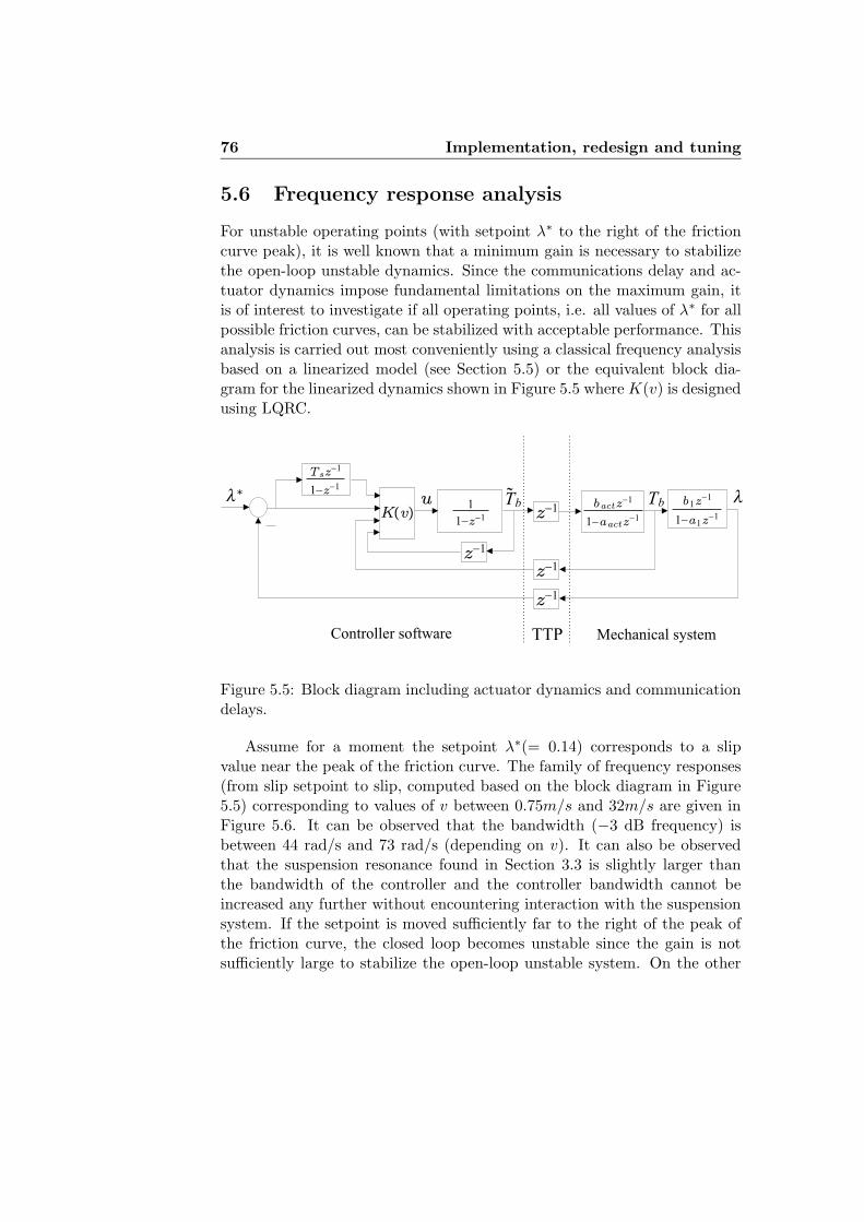
76 Implementation, redesign and tuning
5.6 Frequency response analysis
For unstable operating points (with setpoint λ∗ to the right of the frictioncurve peak), it is well known that a minimum gain is necessary to stabilizethe open-loop unstable dynamics. Since the communications delay and ac-tuator dynamics impose fundamental limitations on the maximum gain, itis of interest to investigate if all operating points, i.e. all values of λ∗ for allpossible friction curves, can be stabilized with acceptable performance. Thisanalysis is carried out most conveniently using a classical frequency analysisbased on a linearized model (see Section 5.5) or the equivalent block dia-gram for the linearized dynamics shown in Figure 5.5 where K(v) is designedusing LQRC.
Controller software TTP Mechanical system
VD
Vz?1
z?1
z?1
z?1
KÝvÞu 1
1?z?1
bactz?1
1?aactz?1
b1z?1
1?a1z?1
Tsz?1
1?z?1
T* b Tb
Figure 5.5: Block diagram including actuator dynamics and communicationdelays.
Assume for a moment the setpoint λ∗(= 0.14) corresponds to a slipvalue near the peak of the friction curve. The family of frequency responses(from slip setpoint to slip, computed based on the block diagram in Figure5.5) corresponding to values of v between 0.75m/s and 32m/s are given inFigure 5.6. It can be observed that the bandwidth (−3 dB frequency) isbetween 44 rad/s and 73 rad/s (depending on v). It can also be observedthat the suspension resonance found in Section 3.3 is slightly larger thanthe bandwidth of the controller and the controller bandwidth cannot beincreased any further without encountering interaction with the suspensionsystem. If the setpoint is moved sufficiently far to the right of the peak ofthe friction curve, the closed loop becomes unstable since the gain is notsufficiently large to stabilize the open-loop unstable system. On the other

5.6 Frequency response analysis 77
Bode Diagram (λ*=0.14)
Frequency (rad/sec)
Pha
se (d
eg)
Mag
nitu
de (d
B)
−60
−40
−20
0
20
System: v1 Sampling time: 0.007 Frequency (rad/sec): 73.7 Magnitude (dB): −2.98
System: v12 Sampling time: 0.007
Frequency (rad/sec): 44.1 Magnitude (dB): −3.03
100 101 102−360
−270
−180
−90
0
90
Increasing v
Increasing v
Figure 5.6: Transfer function from reference to output, when the setpoint isnear the peak of the friction curve.
hand, if the setpoint is moved slightly to the left of the peak (say λ∗ = 0.1)of the friction curve, the family of frequency responses changes to Figure5.7. It is observed that the bandwidth decreases significantly, especially forsmall v, indicating a loss of performance. If the setpoint is moved evenfurther left of the peak, a further loss of performance is experienced. Thus,high performance is achieved only if the setpoint is chosen near the peakof the friction curve. At low friction, the peak is less pronounced and theperformance and the robustness are not expected to be very sensitive tothe choice of setpoint. At high friction, however, the peak is significantand loss of stability will occur if the setpoint is chosen too high, and lossof performance may occur if the setpoint is chosen too low. It must bestressed that this analysis is based on a linearized model and is thereforenot valid for transients that are far from the equilibrium. However, it stillcorrectly points out fundamental limitations in performance and robustness,

78 Implementation, redesign and tuning
Bode Diagram (λ*=0.1)
Frequency (rad/sec)
Pha
se (d
eg)
Mag
nitu
de (d
B)
−50
−40
−30
−20
−10
0
System: v12 Sampling time: 0.007 Frequency (rad/sec): 16.7 Magnitude (dB): −2.99
System: v1 Sampling time: 0.007
Frequency (rad/sec): 0.37 Magnitude (dB): −2.97
10−2 10−1 100 101 102−360
−270
−180
−90
0
Increasing v
Increasing v
Figure 5.7: Transfer function from reference to output, when the setpoint isslightly to the left of the peak of the friction curve.
and suggests useful guidelines for selecting the slip setpoint λ∗, consistentwith underestimation results in (Yi, Alvarez, and Horowitz 2002).
5.7 Improvement of initial transient response
As a result of a slow initial transient response which was discovered in anexperiment on a high friction surface (see Section 6.4), two methods havebeen developed to improve the initial transient response. The first redesignapproach focuses on the initial state of the controller. The second approachis based on the concept of off-equilibrium linearization and design in gainscheduled control.

5.7 Improvement of initial transient response 79
5.7.1 Controller initialization
In the first method, the initial value of the integrator x1(0) is set to avalue corresponding to a nominal steady-state value of the clamping torqueTb which typically is experienced on a given surface. This gives, for thenominal state (with x2 = 0 and x3 = x4 = T ∗
b ), a steady-state considerationleads to
uLQRC = K(v)x = 0 (5.18)
⇓x1(0) = −T ∗
b (k3 + k4)/k1 (5.19)
Because the load is unevenly distributed during braking, it is a need todifferentiate between initialization of front wheels and rear wheels. For thefront wheels
x1(0) = −√
2T ∗b (k3 + k4)/k1 (5.20)
and for the rear wheels
x1(0) =−1√
2T ∗
b (k3 + k4)/k1 (5.21)
Other controller initialization methods are reported in (Kalkkuhl, Jo-hansen, and Ludemann 2002; Ludemann 2002) using a multiple model adap-tive control approach with an estimator resetting rule or by using a µH -estimator such as (Gustafsson 1997; Canudas de Wit, Horowitz, and P.Tsiotras1999) for initialization.
5.7.2 Off-equilibrium scheduling on slip
A second redesign method to improve the initial transient response whenbraking on high µH , off-equilibrium linearization (Johansen, Hunt, Gawthrop,and H.Fritz 1998) with respect to the slip has been applied. The gain ma-trices (5.8) are computed for a finite number of operating points for bothv (5.11) and λ = 0.09, 0.14. In particular, the controller is modified duringtransients at low wheel slip values such that slip setpoint is reached morerapidly. Thus, the controller switches to new gain matrices when the wheelslip is lower than a given threshold, 0.6λ∗. The switching is implementedsimilar to that for bumpless transfer, described in Section 5.8, in order toavoid undesired transients. However, the nominal λ is now on the steep parton the left side of the friction curve peak and, therefore, leads to a highergain near equilibria. Consequently, the transients are speeded up and the

80 Implementation, redesign and tuning
overall performance is improved as shown in the experiment described inSection 6.10. It is remarked that this method has the advantage that it doesnot require an estimate of the equilibrium torque T ∗
b (or µH). Note that theoperating point λ = 0.09 and the wheel slip threshold 0.6λ∗ were selectedby trial and error using the vehicle simulator.
5.8 Bumpless transfer due to controller switching(gain scheduling)
The gain scheduling implemented includes bumpless transfer which is achievedby resetting the integrator, x1, at the switching instants, thereby obtaininga control signal without any discontinuities. At the switching instant, thecommanded clamping torque signal (Tb, the integral value of the control in-put signal u) to the actuator must be constant. This is obtained with thecontrol input signal u set to zero (recall that u is the change in commandedbrake torque, so this essentially requires no jump in the brake torque).
0 = uLQRC(x1(t), x2(t), x3(t), x4(t), v(t), λ(t)) = K(v, λ)x (5.22)
⇓xnew
1 (t) = − (k2x2(t) + k3x3(t) + k4x4(t)) /k1 (5.23)
Bumpless transfer becomes more important the lower the µH is; e.g. onsnow or ice, as the effect of the wheel inertia is more influential.
5.9 Anti-windup
The aim of an anti-windup compensation is to modify the dynamics of thecontrol loop when the control signals saturate. Thus, a good transient be-haviour is attained after de-saturation, while avoiding limit cycle oscillationsand repeated saturations. The technique used here for model-based anti-windup reset is a standard dead-beat anti-windup mechanism (Astrom andWittenmark 1997), where the internal controller states are consistent withthe saturated control input u(t) and the saturated brake torque Tb(t). Sincethere are both a rate and a saturation limit for the brake torque, one way toincorporate this saturation is through the control input u. The anti-windupfor integral of the slip error, x1:
xnew1 (t) = x
′
1(t) +(
Tb(t) − T′
b(t) + uLQRC(t) − uLQ(t))
/k1 (5.24)
5.9 Anti-windup 81
where uLQRC(t) is the rate control input computed by the LQRC, uLQ(t) isthe corresponding unconstrained control and
x′
1(t) = λ(t) − λ(t − 1) (5.25)
T′
b(t) = Tb(t − 1) + uLQRC(t) (5.26)
Tb(t) = Tmaxb ≥ T
′
b(t) ≥ Tminb (5.27)
For the case where no saturation occurs, it can be seen that the nominaldynamics is unchanged as x1 = x
′
1 due to Tb = T′
b and uLQ = uLQRC . Itshould be noticed that this mechanism is also used in the case of controllerinitialization (see Section 5.7.1).

82 Implementation, redesign and tuning
Chapter 6
Experimental Results
This section gives a description of the experimental results obtained with thecontroller described in Section 5. Procedures for testing of an ABS system’sbraking performance in a motor vehicle can be found in publications suchas International Organization for Standardization (ISO) (ISO 1991; ISO1995; ISO 1996; ISO 1999) and in publications of the Society of AutomotiveEngineers (SAE) (SAE 1973). Since this project was aimed at developingan ABS controller for a prototype electro-mechanical wheel brake and notfor a production vehicle, a reduced and simplified test procedure was chosen.
The following subsections describe a series of successful experiments car-ried out for straight-line braking manoeuvre on different road surfaces (ice,snow, dry asphalt, wet asphalt and inhomogeneous asphalt/plastic coatedsurface) and a single experiment carried out for braking in a turn on dryasphalt.
6.1 Experimental scenarios
Table 6.1 gives an overview of the experiments and their order of appearancein this chapter with surface condition, controller configuration and steeringaction for the respective experiment.
For the experiments when braking on ice and snow, the vehicle wasequipped with winter tyres, Conti TS790 215/55R16. All other experimentswere carried out using summer tyres, ContiEcoContact CP 215/55R16. Bothtyre types are produced by Continental.

84 Experimental Results
Test Surface condition λ∗, Slip Commentsno. setpoint
1 Wet inhomogeneous 0.09 Straight2 Dry asphalt 0.09 Straight3 Wet asphalt 0.09 Straight4 Snow 0.07 Straight5 Ice 0.05 Straight6 Dry asphalt 0.14 Turning7 Dry asphalt 0.11 Straight, Controller initialization8 Dry asphalt 0.11 Straight, Off-equilibrium design
Table 6.1: Experimental tests of EMB ABS
6.2 Presentation of experimental results
The following performance criteria are included in the evaluation:
• slip performance w.r.t. slip setpoint (peak, variability, stead-state er-ror)
• lateral stability of vehicle (wheel lock avoided, lateral acceleration)
• deceleration of vehicle
To evaluate the controller performance, mainly the slip behaviour andclamping force are used. From the experimental vehicle, during the experi-ments, the following information was logged for each sample:
• The vehicle speed over ground estimated by the extended Kalman filter(EKF) and measured by an optical correlation sensor.
• The wheel speed for each wheel.
• The estimated wheel slip value for each wheel estimated by the ex-tended Kalman filter.
• Clamping force, desired and measured values.
• Weather condition on the braking surface.
• Slip setpoint.
• Lateral and longitudinal acceleration.

6.3 Wet inhomogeneous surface 85
Other sensor data like the steering wheel angle and the brake pedalposition were also logged, but are omitted for presentation purposes.
For each experiment, there are four plots for each wheel and one plot forthe vehicle.
i. The first plot shows the wheel slip λ (solid line) and the setpoint slipλ∗ (dashed line).
ii. The second plot shows the measured clamping force by the electrome-chanical actuator (solid line) and the desired clamping force from thedriver (dashed line).
iii. The third plot shows the measured wheel speed (solid line) and themeasured vehicle speed (dashed line).
iv. The fourth plot shows the friction curve calculated (see Section 3.2.1)based on the wheel experimental data for the wheel.
v. The fifth plot shows the longitudinal (solid line) and lateral (dashedline) acceleration of the vehicle.
All plots (except the friction curve plot) are plotted with the time onthe x-axis and for vehicle speed v ≥ 1m/s. If the wheel speed v < 1m/s,then the controller is switched off. In the friction curve plot (iv), µ versusλ is plotted, and the figure is therefore limited to the slip values that areexperienced by the wheel during a braking manoeuvre. The analysis of thefriction curve plot is done with reference to (Burckhardt 1993; Canudas deWit, Horowitz, and P.Tsiotras 1999; Gustafsson 1997; Hunter 1998) andSection 3.2.1.
6.3 Wet inhomogeneous surface
Figures 6.1 and 6.2 show braking without any steering manoeuvres on awet asphalt partially covered with a plastic coating. The initial speed isv(0) = 22 m/s and the slip setpoint is λ∗ = 0.09.
6.3.1 Slip
Observe that there is significant variability in the slip for t ≤ 6s, whereasfor t > 6s, the regulation is satisfactory. The variability is expected tobe mainly due to the inhomogeneous road surface that provides externaldisturbances to the system. The peak slip value λ ≈ 0.45 for t = 3.7s.

86 Experimental Results
6.3.2 Lateral stability
The lateral acceleration shown in Figure 6.2 is negligible.
6.3.3 Deceleration of vehicle
A deceleration of 3m/s2 is reached very quickly and maintained during brak-ing.
6.3.4 Friction estimate
The friction curve plot in Figure 6.1 shows a friction peak value µH ≈ 0.5 forλ = 0.07− 0.1. Its shape, limited to a maximum slip of λ < 0.45, resemblesthe friction curve for µH = 0.5 shown in Figure 3.2.
6.3.5 Controller performance
The transient performance is fast and the overall controller performance issatisfactory considering the road surface.
6.4 Dry asphalt
Figures 6.3-6.5 show experimental results with braking on dry asphalt. Theinitial speed is v(0) = 21 m/s, the slip setpoint is λ∗ = 0.09.
6.4.1 Slip
As the speed approaches zero, some variability in the slip emerges. Theclamping force does not oscillate, this is probably due to the sensor noisethat is known to increase as the speed approaches zero (see Section 3.1). Theslip is too low and the resulting friction force is too low in the intervals 0.2 ≤t ≤ 0.7 and 0.2 ≤ t ≤ 0.4 for the front and rear wheels respectively, leading toan unnecessarily large braking distance. This is due to the significant modelinaccuracy in the low-slip region due to the friction curve being linearized inthe control design, cf. Figure 3.2. The peak slip value (front wheel) λ ≈ 0.2for t = 2.5s.
6.4.2 Lateral stability
The lateral acceleration shown in Figure 6.5 is negligible.

6.4 Dry asphalt 87
0 1 2 3 4 5 6 7 80
0.1
0.2
0.3
0.4
0.5
0.6
0.7
0.8
0.9
1
t, [s]
Slip (λ, λ*=0.09)
0 1 2 3 4 5 6 7 80
0.2
0.4
0.6
0.8
1
1.2
1.4
1.6
1.8
2x 10
4
t, [s]
Clamping Force: ABS(u, solid), Driver(Fb, dashed)
0 1 2 3 4 5 6 7 80
5
10
15
20
25
t, [s]
Speed: Wheel (ωr, solid) & Vehicle (v, dashed)
0 0.2 0.4 0.6 0.8 10
0.1
0.2
0.3
0.4
0.5
0.6
0.7
0.8
0.9
1
λ
Friction Curve µ (filtered, solid)
Figure 6.1: Wet inhomogeneous surface, front left wheel

88 Experimental Results
0 1 2 3 4 5 6 7 8−12
−10
−8
−6
−4
−2
0
2
4
t, [s]
Acceleration: ax(solid), a
y(dashed), [m/s2]
Figure 6.2: Wet inhomogeneous surface, car

6.4 Dry asphalt 89
0 0.5 1 1.5 2 2.50
0.1
0.2
0.3
0.4
0.5
0.6
0.7
0.8
0.9
1
t, [s]
Slip (λ, λ*=0.09)
0 0.5 1 1.5 2 2.50
0.5
1
1.5
2
2.5x 10
4
t, [s]
Clamping Force: ABS(u, solid), Driver(Fb, dashed)
0 0.5 1 1.5 2 2.50
5
10
15
20
25
t, [s]
Speed: Wheel (ωr, solid) & Vehicle (v, dashed)
0 0.2 0.4 0.6 0.8 10
0.1
0.2
0.3
0.4
0.5
0.6
0.7
0.8
0.9
1
λ
Friction Curve µ (filtered, solid)
Figure 6.3: Dry asphalt, front left wheel

90 Experimental Results
0 0.5 1 1.5 2 2.50
0.1
0.2
0.3
0.4
0.5
0.6
0.7
0.8
0.9
1
t, [s]
Slip (λ, λ*=0.09)
0 0.5 1 1.5 2 2.50
0.5
1
1.5
2
2.5x 10
4
t, [s]
Clamping Force: ABS(u, solid), Driver(Fb, dashed)
0 0.5 1 1.5 2 2.50
5
10
15
20
25
t, [s]
Speed: Wheel (ωr, solid) & Vehicle (v, dashed)
0 0.2 0.4 0.6 0.8 10
0.1
0.2
0.3
0.4
0.5
0.6
0.7
0.8
0.9
1
λ
Friction Curve µ (filtered, solid)
Figure 6.4: Dry asphalt, rear right wheel

6.4 Dry asphalt 91
0 0.5 1 1.5 2 2.5−12
−10
−8
−6
−4
−2
0
2
4
6
t, [s]
Acceleration: ax(solid), a
y(dashed), [m/s2]
Figure 6.5: Dry asphalt, car

92 Experimental Results
6.4.3 Deceleration of vehicle
Figure 6.5 shows that a high deceleration value, ax = 9−10m/s2, is reachedand maintained for t > 0.6s, approximately 0.4s after braking commences.
6.4.4 Friction estimate
The friction curve plots for both the front and the rear wheels are shownin Figures 6.3 and 6.4, respectively. The figures resemble the dry asphaltfriction plot in Figure 3.2 for µH ≈ 0.9. The friction peak occurs for λ =0.05− 0.2 and with a value of µ = 0.9. The friction curves’s complete shapecannot be produced as slip λ < 0.2, but they indicate that the brake forceused corresponds to braking on dry asphalt.
6.4.5 Controller performance
It is important to note that the regulation is highly accurate and satisfactory.Observe that the transient performance is not as fast as experienced inSection 6.4 mainly because the steady-state value of the clamping forceis further away from its initial state. Consequently, the initial transientresponse is not satisfactory as the clamping force does not increase fastenough. A redesign of the slip controller is necessary and two approacheswere presented in Sections 5.7.1 and 5.7.2, and their experimental resultsare presented in Sections 6.9 and 6.10.
6.5 Wet asphalt
Figures 6.6-6.7 show experimental results with braking on wet asphalt. Theinitial speed is v(0) = 23 m/s and the slip setpoint is λ∗ = 0.09.
6.5.1 Slip
Significantly less variability in the slip is observed than for the wet inho-mogeneous case (see Section 6.3). The peak slip value λ ≈ 0.4 for t = 3.1sexcept when the velocity becomes very small. The initial slip variability ismainly due to an inhomogeneous road surface that provides external distur-bances to the system.
6.5.2 Lateral stability
The lateral acceleration shown in Figure 6.7 is negligible.

6.5 Wet asphalt 93
0 1 2 3 4 5 6 7 80
0.1
0.2
0.3
0.4
0.5
0.6
0.7
0.8
0.9
1
t, [s]
Slip (λ, λ*=0.09)
0 1 2 3 4 5 6 7 80
0.2
0.4
0.6
0.8
1
1.2
1.4
1.6
1.8
2x 10
4
t, [s]
Clamping Force: ABS(u, solid), Driver(Fb, dashed)
0 1 2 3 4 5 6 7 80
5
10
15
20
25
t, [s]
Speed: Wheel (ωr, solid) & Vehicle (v, dashed)
0 0.2 0.4 0.6 0.8 10
0.1
0.2
0.3
0.4
0.5
0.6
0.7
0.8
0.9
1
λ
Friction Curve µ (filtered, solid)
Figure 6.6: Wet asphalt, front left wheel

94 Experimental Results
0 1 2 3 4 5 6 7 8−12
−10
−8
−6
−4
−2
0
2
4
t, [s]
Acceleration: ax(solid), a
y(dashed), [m/s2]
Figure 6.7: Wet asphalt, car

6.6 Snow 95
6.5.3 Deceleration of vehicle
Figure 6.7 shows that deceleration stays between 2 − 4m/s2 and reaches4m/s2 approximately 0.25s after braking commences.
6.5.4 Friction estimate
The friction curve plots for the front wheel is shown in Figure 6.6. It issimilar to the friction curve found for the wet, inhomogeneous surface inFigure 6.1. The friction peak occurs for λ = 0.05 − 0.1 and with a value ofµH ≈ 0.5. Its shape resembles the wet, asphalt friction curve seen in Figure3.2 for µH = 0.5 and thus, the brake force used in this case corresponds tobraking on wet asphalt.
6.5.5 Controller performance
Observe that the transient performance is again much better than on dryasphalt (see Section 6.4), mainly because the steady-state value of the clamp-ing force is closer to its initial state. Overall, the controller performs satis-factorily.
6.6 Snow
Figures 6.8-6.10 show a straight-line braking manoeuvre on a road coveredwith 3 cm of fresh snow. The vehicle speed is v = 22m/s when brakingis commenced and without any steering manoeuvres. The slip set point isλ∗ = 0.07.
6.6.1 Slip
The rear wheel slip, Figure 6.9, is slightly more oscillatory than the frontwheel slip in Figure 6.8. The slip peak (rear) is approximately 0.25 andoccurs at low speed (three places) for 5.8s < t < 7.2s. The front slip peakis 0.6, but happens at low speed (< 2.5m/s) for t = 7.2s.
6.6.2 Lateral stability
The lateral acceleration and velocity shown in Figure 6.10 are negligible.

96 Experimental Results
0 1 2 3 4 5 6 70
0.1
0.2
0.3
0.4
0.5
0.6
0.7
0.8
0.9
1
t, [s]
Slip (λ, λ*=0.07)
0 1 2 3 4 5 6 70
5000
10000
15000
t, [s]
Clamping Force: ABS(u, solid), Driver(Fb, dashed)
0 1 2 3 4 5 6 70
5
10
15
20
25
t, [s]
Speed: Wheel (ωr, solid) & Vehicle (v, dashed)
0 0.2 0.4 0.6 0.8 10
0.1
0.2
0.3
0.4
0.5
0.6
0.7
0.8
0.9
1
λ
Friction Curve µ (filtered, solid)
Figure 6.8: Snow, front left wheel

6.6 Snow 97
0 1 2 3 4 5 6 70
0.1
0.2
0.3
0.4
0.5
0.6
0.7
0.8
0.9
1
t, [s]
Slip (λ, λ*=0.07)
0 1 2 3 4 5 6 70
5000
10000
15000
t, [s]
Clamping Force: ABS(u, solid), Driver(Fb, dashed)
0 1 2 3 4 5 6 70
5
10
15
20
25
t, [s]
Speed: Wheel (ωr, solid) & Vehicle (v, dashed)
0 0.2 0.4 0.6 0.8 10
0.1
0.2
0.3
0.4
0.5
0.6
0.7
0.8
0.9
1
λ
Friction Curve µ (filtered, solid)
Figure 6.9: Snow, rear right wheel

98 Experimental Results
0 1 2 3 4 5 6 7−8
−7
−6
−5
−4
−3
−2
−1
0
1
2
t, [s]
Acceleration: ax(solid), a
y(dashed), [m/s2]
Figure 6.10: Snow, car

6.7 Ice 99
6.6.3 Deceleration of vehicle
A deceleration of 3m/s2 is reached and maintained 0.3s after braking com-mences.
6.6.4 Friction estimate
The maximum friction coefficient is µH ≈ 0.3 cf. Figure 6.8. A slightlyhigher friction value is obtained for the rear wheel than for the front wheel.Both wheels achieve maximum friction at λ ≈ 0.05 − 0.10.
6.6.5 Controller performance
The transient performance is satisfactory and the regulation is excellent.
6.7 Ice
Figures 6.11-6.13 show a straight-line braking manoeuvre on an icy road.The vehicle speed is v(0) = 16m/s when braking commences. The slip setpoint is λ∗ = 0.05.
6.7.1 Slip
The front wheel slip peak, λ = 0.3, is at t = 8.3s and for the rear wheel,λ = 0.45, at t = 9.2s. This occurs at low velocity, where the slip dynamicsare more sensitive.
6.7.2 Lateral stability
In Figure 6.13, ay changes suddenly by 2m/s2 at around t = 4s , from−1m/s2 to 1m/s2. The lateral acceleration ay = 2m/s2 is maintained for2s.
6.7.3 Deceleration of vehicle
A deceleration of 2 − 3m/s2 is reached and maintained 0.5s after brakingcommences.

100 Experimental Results
0 2 4 6 80
0.1
0.2
0.3
0.4
0.5
0.6
0.7
0.8
0.9
1
t, [s]
Slip (λ, λ*=0.05)
0 2 4 6 80
1000
2000
3000
4000
5000
6000
7000
8000
9000
10000
t, [s]
Clamping Force: ABS(u, solid), Driver(Fb, dashed)
0 2 4 6 80
2
4
6
8
10
12
14
16
t, [s]
Speed: Wheel (ωr, solid) & Vehicle (v, dashed)
0 0.2 0.4 0.6 0.8 10
0.1
0.2
0.3
0.4
0.5
0.6
0.7
0.8
0.9
1
λ
Friction Curve µ (filtered, solid)
Figure 6.11: Ice, front left wheel

6.7 Ice 101
0 2 4 6 80
0.1
0.2
0.3
0.4
0.5
0.6
0.7
0.8
0.9
1
t, [s]
Slip (λ, λ*=0.05)
0 2 4 6 80
1000
2000
3000
4000
5000
6000
7000
8000
9000
10000
t, [s]
Clamping Force: ABS(u, solid), Driver(Fb, dashed)
0 2 4 6 80
2
4
6
8
10
12
14
16
t, [s]
Speed: Wheel (ωr, solid) & Vehicle (v, dashed)
0 0.2 0.4 0.6 0.8 10
0.1
0.2
0.3
0.4
0.5
0.6
0.7
0.8
0.9
1
λ
Friction Curve µ (filtered, solid)
Figure 6.12: Ice, rear right wheel

102 Experimental Results
0 2 4 6 8−6
−5
−4
−3
−2
−1
0
1
2
t, [s]
Acceleration: ax(solid), a
y(dashed), [m/s2]
Figure 6.13: Ice, car

6.8 Turning on dry asphalt 103
6.7.4 Friction estimate
The maximum friction coefficient is approximately µH ≈ 0.15−0.20. This isseen in the friction curve plots 6.11 and 6.12, with a slightly higher frictionvalue obtained for the rear wheel. Both wheels reach maximum friction atλ ≈ 0.02.
6.7.5 Controller performance
Braking on ice gives similar performance to that of braking on snow. At suchlow friction levels for both the wheel slip and the clamping force, the controlsystem becomes very sensitive specially to disturbances due to an inhomo-geneous road surface which is more likely to happen on ice. This can be seenas slip disturbances or with a split friction surface, a side acceleration of thevehicle. At such low wheel slip and clamping force levels, the control systemis also sensitive towards disturbances in sensor noise, actuator inaccuracies,nonlinearities due to internal friction and other phenomena. The transientperformance is satisfactory and the regulation is excellent.
6.8 Turning on dry asphalt
Figures 6.14-6.18 show a braking manoeuvre in a turn where the vehicle isdriven clockwise in a circle with a radius of approximately 15m. The initialspeed v(0) = 15m/s and the initial lateral acceleration ay ≈ 8m/s2.In thespeed figures for Figure 6.14-6.17, it can be seen that the estimation by theextended Kalman-filter of the vehicle speed is either 0.5m/s higher or lowercompared to the wheel perimeter speed, when the vehicle is not braking.This is due to the fact that the outer wheels rotate faster than the innerwheels.
6.8.1 Slip
The outer front left wheel is locked for 2.05s < t < 2.2s, see Figure 6.14. Asimilar situation occurs for the outer rear left wheel, but the slip peak reaches0.8. The slip for the inner wheels λ < 0.25 throughout the manoeuvre.
6.8.2 Lateral stability
Figure 6.18 shows that the lateral acceleration decreases steadily duringthe braking manoeuvre, while the oscillations in ax and also in ay, indicatepitching and rolling movements of the vehicle. The approximately constant
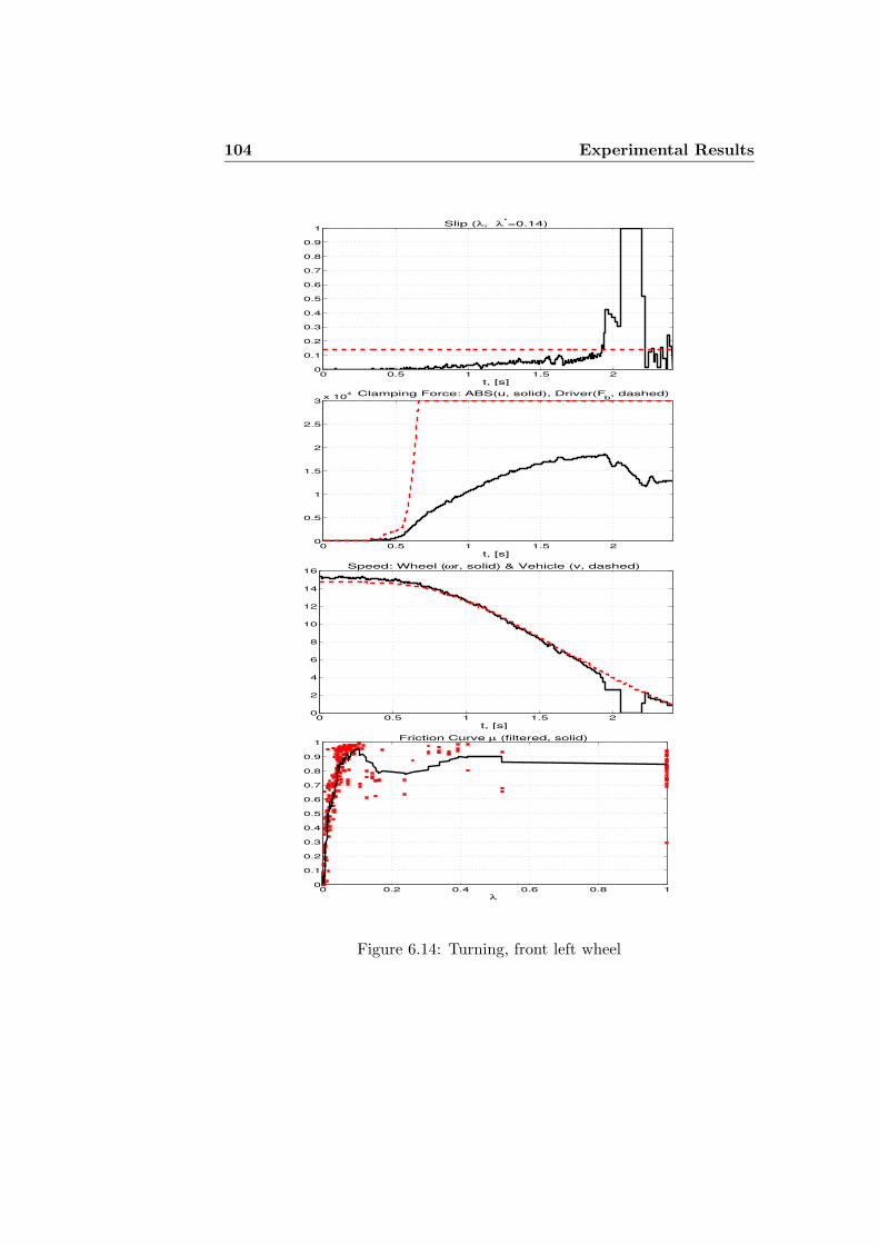
104 Experimental Results
0 0.5 1 1.5 20
0.1
0.2
0.3
0.4
0.5
0.6
0.7
0.8
0.9
1
t, [s]
Slip (λ, λ*=0.14)
0 0.5 1 1.5 20
0.5
1
1.5
2
2.5
3x 10
4
t, [s]
Clamping Force: ABS(u, solid), Driver(Fb, dashed)
0 0.5 1 1.5 20
2
4
6
8
10
12
14
16
t, [s]
Speed: Wheel (ωr, solid) & Vehicle (v, dashed)
0 0.2 0.4 0.6 0.8 10
0.1
0.2
0.3
0.4
0.5
0.6
0.7
0.8
0.9
1
λ
Friction Curve µ (filtered, solid)
Figure 6.14: Turning, front left wheel

6.8 Turning on dry asphalt 105
0 0.5 1 1.5 20
0.1
0.2
0.3
0.4
0.5
0.6
0.7
0.8
0.9
1
t, [s]
Slip (λ, λ*=0.14)
0 0.5 1 1.5 20
0.5
1
1.5
2
2.5
3x 10
4
t, [s]
Clamping Force: ABS(u, solid), Driver(Fb, dashed)
0 0.5 1 1.5 20
2
4
6
8
10
12
14
16
t, [s]
Speed: Wheel (ωr, solid) & Vehicle (v, dashed)
0 0.2 0.4 0.6 0.8 10
0.1
0.2
0.3
0.4
0.5
0.6
0.7
0.8
0.9
1
λ
Friction Curve µ (filtered, solid)
Figure 6.15: Turning, front right wheel

106 Experimental Results
0 0.5 1 1.5 20
0.1
0.2
0.3
0.4
0.5
0.6
0.7
0.8
0.9
1
t, [s]
Slip (λ, λ*=0.14)
0 0.5 1 1.5 20
0.5
1
1.5
2
2.5
3x 10
4
t, [s]
Clamping Force: ABS(u, solid), Driver(Fb, dashed)
0 0.5 1 1.5 20
2
4
6
8
10
12
14
16
t, [s]
Speed: Wheel (ωr, solid) & Vehicle (v, dashed)
0 0.2 0.4 0.6 0.8 10
0.1
0.2
0.3
0.4
0.5
0.6
0.7
0.8
0.9
1
λ
Friction Curve µ (filtered, solid)
Figure 6.16: Turning, rear left wheel

6.8 Turning on dry asphalt 107
0 0.5 1 1.5 20
0.1
0.2
0.3
0.4
0.5
0.6
0.7
0.8
0.9
1
t, [s]
Slip (λ, λ*=0.14)
0 0.5 1 1.5 20
0.5
1
1.5
2
2.5
3x 10
4
t, [s]
Clamping Force: ABS(u, solid), Driver(Fb, dashed)
0 0.5 1 1.5 20
2
4
6
8
10
12
14
16
t, [s]
Speed: Wheel (ωr, solid) & Vehicle (v, dashed)
0 0.2 0.4 0.6 0.8 10
0.1
0.2
0.3
0.4
0.5
0.6
0.7
0.8
0.9
1
λ
Friction Curve µ (filtered, solid)
Figure 6.17: Turning, rear right wheel

108 Experimental Results
0 0.5 1 1.5 2−12
−10
−8
−6
−4
−2
0
2
4
6
t, [s]
Acceleration: ax(solid), a
y(dashed), [m/s2]
Figure 6.18: Turning, car

6.9 Dry asphalt, controller initialization 109
lateral acceleration confirms together with the slip that the vehicle is steer-able during the manoeuvre. The lateral acceleration ay decreases steadilyuntil it reaches zero at t = 1.9s and remains at zero until the vehicle comesto a standstill at approximately t ≈ 2.5s.
6.8.3 Deceleration of vehicle
Figure 6.18 shows the vehicle reaching a deceleration of 8 − 10m/s2 and ismaintained 0.5s after braking commences.
6.8.4 Friction estimate
The friction curve plots for the two front and the two rear wheels are shownin Figures 6.14-6.17, respectively. The theory for calculating the frictioncurve (see Section 3.2.1) for braking while turning requires that the vehicleside slip angle, the wheel turn angle and the vehicle yaw rate are known. Asthe vehicle side slip angle is not known, only the longitudinal friction can becalculated and the friction curve is therefore only an approximation. Thefriction peak, µH = 0.9, occurs for λ = 0.05 − 0.2.
6.8.5 Controller performance
The controller transient response is very slow as the clamping force doesnot increase fast enough (for all the wheels). Consequently, the slip is toolow and the resulting friction force is too low for the whole braking periodleading to an unnecessarily large braking distance. This is principally dueto the significant model inaccuracy occurring for side slips where α > 0 andsmall λ. Notice that the linearization underlying the control design is donewith the side slip α = 0, cf. Figure 3.2.
6.9 Dry asphalt, controller initialization
This first redesign idea is based on the fact that the initial state of thecontroller will play an important role in the initial transient, see Section5.7.1. For the dry asphalt experiment shown in Figures 6.19-6.21, the slipsetpoint is λ∗ = 0.11 and the initial speed is v(0) = 30m/s.
6.9.1 Slip
The front wheel slip peak, λ = 0.7, is at t = 1.2s when the wheel slipcontroller is activated. For the rear wheel, the slip peak value λ ≈ 0.2
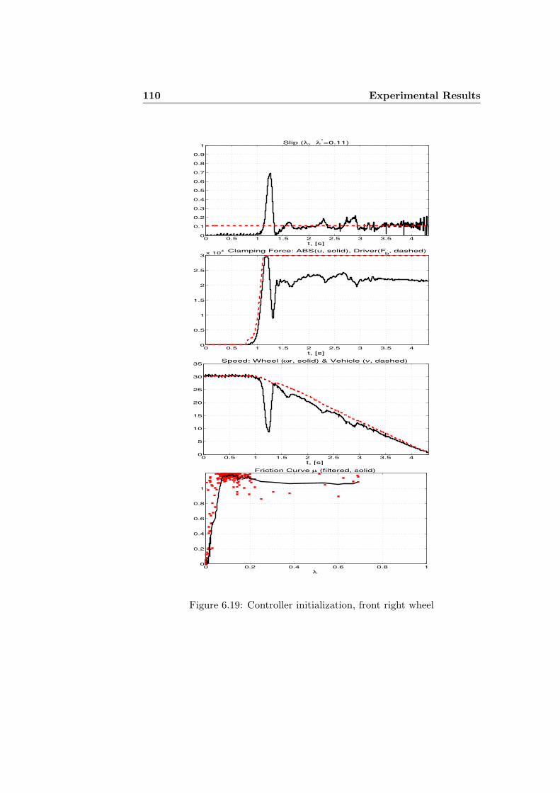
110 Experimental Results
0 0.5 1 1.5 2 2.5 3 3.5 40
0.1
0.2
0.3
0.4
0.5
0.6
0.7
0.8
0.9
1
t, [s]
Slip (λ, λ*=0.11)
0 0.5 1 1.5 2 2.5 3 3.5 40
0.5
1
1.5
2
2.5
3x 10
4
t, [s]
Clamping Force: ABS(u, solid), Driver(Fb, dashed)
0 0.5 1 1.5 2 2.5 3 3.5 40
5
10
15
20
25
30
35
t, [s]
Speed: Wheel (ωr, solid) & Vehicle (v, dashed)
0 0.2 0.4 0.6 0.8 10
0.2
0.4
0.6
0.8
1
λ
Friction Curve µ (filtered, solid)
Figure 6.19: Controller initialization, front right wheel

6.9 Dry asphalt, controller initialization 111
0 0.5 1 1.5 2 2.5 3 3.5 40
0.1
0.2
0.3
0.4
0.5
0.6
0.7
0.8
0.9
1
t, [s]
Slip (λ, λ*=0.11)
0 0.5 1 1.5 2 2.5 3 3.5 40
0.5
1
1.5
2
2.5
3x 10
4
t, [s]
Clamping Force: ABS(u, solid), Driver(Fb, dashed)
0 0.5 1 1.5 2 2.5 3 3.5 40
5
10
15
20
25
30
35
t, [s]
Speed: Wheel (ωr, solid) & Vehicle (v, dashed)
0 0.2 0.4 0.6 0.8 10
0.2
0.4
0.6
0.8
1
λ
Friction Curve µ (filtered, solid)
Figure 6.20: Controller initialization, rear right wheel

112 Experimental Results
0 0.5 1 1.5 2 2.5 3 3.5 4−12
−10
−8
−6
−4
−2
0
2
4
6
t, [s]
Acceleration: ax(solid), a
y(dashed), [m/s2]
Figure 6.21: Controller initialization, car

6.10 Dry asphalt, off-equilibrium design 113
occurs at low velocity, where the slip dynamics are more sensitive.
6.9.2 Lateral stability
The lateral acceleration shown in Figure 6.21 is negligible.
6.9.3 Deceleration of vehicle
Deceleration is between 8− 10m/s2, see Figure 6.21, and is maintained 0.5safter braking commences.
6.9.4 Friction estimate
The friction curve plots for both the front and the rear wheels are shownin Figures 6.19 and 6.20, respectively. The figures’s shape resemble the dryasphalt friction plot in Figure 3.2 for µH ≈ 0.9. The friction peak occursfor λ = 0.1 and with a value of µ ≈ 1.2.
6.9.5 Controller performance
When the wheel slip controller is activated, the initial state of the integratorx1(0) is set to a value that corresponds to the nominal steady-state clampingtorque typically experienced on dry asphalt. Notice that the initial transientis significantly improved, but with an overshoot that might be eliminatedby more accurate initialization (along the ideas in (Kalkkuhl, Johansen,Ludemann, and Queda 2001; Kalkkuhl, Johansen, and Ludemann 2002)).Note that since the experiment was conducted on dry asphalt with a highslip setpoint, the rear wheel brake torques saturate throughout the brakingperiod without achieving the specified slip setpoint. Thus, the performanceof the controller for the rear wheel cannot be evaluated.
6.10 Dry asphalt, off-equilibrium design
The second redesign idea is based on the concept of off-equilibrium lineariza-tion and design in gain scheduled control (see Section 5.7.2).
Figures 6.22-6.24 show experimental results with braking on dry asphaltwith a modified controller to improve the initial response. The initial speedis v(0) = 30m/s and the slip setpoint is λ∗ = 0.11.

114 Experimental Results
0 0.5 1 1.5 2 2.5 3 3.50
0.1
0.2
0.3
0.4
0.5
0.6
0.7
0.8
0.9
1
t, [s]
Slip (λ, λ*=0.11)
0 0.5 1 1.5 2 2.5 3 3.50
0.5
1
1.5
2
2.5
3x 10
4
t, [s]
Clamping Force: ABS(u, solid), Driver(Fb, dashed)
0 0.5 1 1.5 2 2.5 3 3.50
5
10
15
20
25
30
35
t, [s]
Speed: Wheel (ωr, solid) & Vehicle (v, dashed)
0 0.2 0.4 0.6 0.8 10
0.1
0.2
0.3
0.4
0.5
0.6
0.7
0.8
0.9
1
λ
Friction Curve µ (filtered, solid)
Figure 6.22: Off-equilibrium design, front left wheel

6.10 Dry asphalt, off-equilibrium design 115
0 0.5 1 1.5 2 2.5 3 3.50
0.1
0.2
0.3
0.4
0.5
0.6
0.7
0.8
0.9
1
t, [s]
Slip (λ, λ*=0.11)
0 0.5 1 1.5 2 2.5 3 3.50
0.5
1
1.5
2
2.5
3x 10
4
t, [s]
Clamping Force: ABS(u, solid), Driver(Fb, dashed)
0 0.5 1 1.5 2 2.5 3 3.50
5
10
15
20
25
30
35
t, [s]
Speed: Wheel (ωr, solid) & Vehicle (v, dashed)
0 0.2 0.4 0.6 0.8 10
0.1
0.2
0.3
0.4
0.5
0.6
0.7
0.8
0.9
1
λ
Friction Curve µ (filtered, solid)
Figure 6.23: Off-equilibrium design, rear right wheel

116 Experimental Results
0 0.5 1 1.5 2 2.5 3 3.5−20
−15
−10
−5
0
5
t, [s]
Acceleration: ax(solid), a
y(dashed), [m/s2]
Figure 6.24: Off-equilibrium design, car

6.11 Experimental problems 117
6.10.1 Slip
The front wheel slip peak, λ = 0.65, is at t = 0.7s. For the rear wheel, theslip peak value λ ≈ 0.35 occurs at low velocity, where the slip dynamics aremore sensitive.
6.10.2 Lateral stability
The lateral acceleration shown in Figure 6.24 is negligible.
6.10.3 Deceleration of vehicle
Deceleration reaches 8 − 10m/s2 0.3s after braking commences, see Figure6.24, and this is then maintained.
6.10.4 Friction estimate
The friction curve plots for the front and the rear wheels are shown respec-tively in Figures 6.22 and 6.23. The figures resemble the dry asphalt frictionplot in Figure 3.2 for µH ≈ 0.9. The friction peak occurs for λ = 0.1 andwith a value of µ = 0.95.
6.10.5 Controller performance
As a result of the modification of the controller during transients at lowwheel slip values, it appears that the setpoint is reached more rapidly. Thecontroller switches to new gain matrices when the wheel slip λ is lower than agiven threshold, namely 0.6λ∗. Since the nominal λ is now on the steep parton the left side of the friction curve peak, this leads to a higher gain thannear equilibria. As a result, the transients are speeded up and the overallperformance is improved. Again, there is some initial overshoot, which couldbe reduced by fine-tuning the switching thresholds and the off-equilibriumcontrol design.
It should be noticed that the driver eases the brake pedal at t = 0.9s.This affects only the performance of the rear wheel, see Figure 6.23.
6.11 Experimental problems
Rear wheel hardware problems occurred in experiments 1 and 3 (Sections6.3 and 6.5), and no log-data was produced. Thus, for the experimentsno.1 and 3, there are no figures showing the performance of the rear wheel

118 Experimental Results
controllers. In general, the performances achieved for the rear wheel slipcontrollers were better than those achieved for the front.
In experiment no.6 (Section 6.8) the speed figure for the front right wheel(see Figure 6.15), has a wheel speed noise (spikes) equivalent to 6% of thevehicle speed for t < 0.6s.
In experiment no.7 (Section 6.9), the friction curve plots shown in Figures6.19 and 6.20, indicate an error in the logged values (or in the model) asthe estimated friction curves have a positive offset of ≈ 0.3 versus the valuesexperienced on other dry asphalt tests.

Chapter 7
Conclusions
In this thesis, several topics within control design and robustness, and stabil-ity analysis of a model-based wheel slip controller, together with a detailedexperimental evaluation using a test vehicle have been addressed. The over-all goal has been to investigate robustness through analysis and experimentsusing a recently developed controller design theory - explicit sub-optimal lin-ear quadratic regulation with state and input constraints. Using Lyapunovtheory, frequency analysis and experimental verifications, performance androbustness of a gain scheduled nonlinear wheel slip controller for a vehicleequipped with electromechanical brakes has been studied.
Despite the fact that the wheel slip dynamics are highly nonlinear, thecontrol design relies on local linearization and gain scheduling. A controlsystem containing just the slip dynamics is shown to be uniformly expo-nentially stable with a large region of attraction using Lyapunov theory.Since this controller cannot be implemented without significant loss of per-formance due to the dependency of the knowledge of the friction coefficient,a second control system including integral action (to eliminate steady-statefriction uncertainties) is shown to be locally uniformly exponentially stableusing Lyapunov theory and robust to the uncertain road/tyre friction. Athird control system is then studied, also including an actuator model. Aparameter-dependent Lyapunov function for the nominal linear parametervarying closed loop system is found by solving a linear matrix inequality(LMI) problem. This function is investigated for robustness with respectto uncertainty in the road/tyre friction characteristic. Unfortunately, theLMI approach does not allow a rigorous conclusion, except local stability,since the Lyapunov-function candidate at hand appears to be conservative.However, the analysis indicates that the observations agree well with the

120 Conclusions
experience from simulations and experiments.The fundamental limitations of performance are the TTP communication
delay, the actuator dynamics (both which introduce phase losses) and thechoice of open loop unstable slip setpoints. These limitations are analyzedusing classical frequency analysis based on a linearized model. It is shownthat high performance is obtained if the slip setpoint is chosen near thefriction peak. For high friction, loss of stability will occur if slip setpoint ischosen too high or loss of performance if the slip setpoint is chosen too low.The communication delay will be reduced in the future as future systemsmay be using FlexRay, a communication protocol with a higher samplingrate than the TTP used in the test vehicle in this project. It should also benoted that the extended Kalman filter introduces estimator errors that maystrongly influence the performance.
The experiments using a test vehicle show an accurate regulation of thewheel slip is feasible for a range of desired setpoints under a wide rangeof road conditions. A test scenario where braking in a turn is performedyields unsatisfactory performance as the model is linearized for straight-linebraking. Although the design and experiments have been carried out for avehicle with drive-by-wire system, the main ideas are believed to be suitablefor conventional hydraulic and electro-hydraulic brakes actuators, and theirsensory systems. Slip peaking, which occurs in production cars equippedwith conventional ABS systems, reduces the driving comfort significantly.The model-based approach presented in this thesis, is more comfortable,yields better performance and does not rely on strong knowledge of thetyre/road friction curve. Moreover, a highly beneficial feature of this model-based design approach is the modest time taken to design and tune the wheelslip controller. The approach is also modular as the wheel slip controller canbe combined with different estimation algorithms, actuators and supervisorycontrol systems. Nevertheless, do note that conventional ABS systems arevery robust.
Results from (Ludemann 2002) for the controller designs used in the H2Cproject show that the controller performances converge. This again indicatesthat the LQRC control design used in this thesis yields similar performanceas the PI controller used by (Ludemann 2002; Solyom and Rantzer 2002;Wang, Schmitt-Hartmann, Schinkel, and Hunt 2001).
The experimental results and the respective test scenarios presented inthis thesis were not duplicated so as to analyze repeatability, due to limitedaccess to the test vehicle, as the LQRC wheel slip controller therefore couldnot be optimally tuned. But, there are no foreseen problems causing non-repeatability.

7.1 Future works 121
As there is room for further improvements and extensions of the wheelslip control approach, a summary for future works is given in the followingsection.
7.1 Future works
The issues of interest listed for future works below contain both theoreticaland practical aspects. The model used in this thesis for controller design isimplemented and tested in a test vehicle. Since the H2C project was aimedat developing an ABS controller for a prototype electro-mechanical wheelbrake, a reduced and simplified test procedure was chosen as the controllerswere not intended for production vehicles. To fully validate the proposedcontrollers, a more extended test program is needed, with both sufficientaccess to the test vehicle and more test scenarios as specified in some ISOand SAE documents (see Chapter 6). A list of topics for further research islisted below.
i. The control design presented in this thesis is only focused on longi-tudinal slip. It is the belief of the author that the slip control designcan easily be extended for control problems such as lateral (side-slip)and yaw control cases, e.g. ESP. A similar problem that should beaddressed is split-friction-coefficient surfaces.
ii. Unmodelled dynamics such as pitching and suspension should be takenmore directly into account in the control design to improve the con-troller performance. Further, unmodelled dynamics such as brake in-teraction through the chassis should also be considered.
iii. An analytical analysis of a gain scheduled LQ using Lyapunov/LMIfor the slip model including the actuator dynamics should be sought,although this has been tried unsuccessfully by the author due to thecomplex solution.
iv. Performance improvements expected when braking in a turn, withgain scheduling applied on side-slip α. Further, gain scheduling on thefriction coefficient (µH) between tyre and road should yield significantreductions in the slip and clamping force transients on inhomogeneoussurfaces.
v. To improve the initial controller performance for high friction surfaces(i.e. dry asphalt), a more accurate initialization strategy similar to

122 Conclusions
what was done in (Kalkkuhl, Johansen, Ludemann, and Queda 2001;Kalkkuhl, Johansen, and Ludemann 2002; Ludemann 2002) should beimplemented.
vi. There is room for improved performance with tuning, especially forthe off-equilibrium design.
vii. With faster CPU (BBWM) and more memory, a more refined gainscheduling should be possible.

Bibliography
Anderson, B. D. O. and J. B. Moore (1989). Optimal control : linearquadratic methods. Prentice-Hall.
Astrom, K. J. and B. Wittenmark (1997). Computer Controlled Systems:theory and design (Third ed.). Prentice-Hall.
Bakker, E., L. Nyborg, and H. B. Pacejka (1987). Tyre modelling forUse in Vehicle Dynamic Studies. Technical Report 870421, Society ofAutomotive Engineers, Warrendale PA.
Bemporad, A., K. Fukuda, and F. D. Torrisi (2001). Convexity recognitionof the union of polyhedra. Computational Gemometry 18, 141–154.
Bemporad, A., M. Morari, V. Dua, and E. Pistikopoulos (2000). Theexplicit solution of model predictive control via multiparametricquadratic programming. In Proc. American Contr. Conf., Chicago,Volume 2, pp. 872–876.
Bemporad, A., M. Morari, V. Dua, and E. N. Pistikopoulos (2002). Theexplicit linear quadratic regulator for constrained systems. Automat-ica 38, 3–20.
Boyd, S., V. Balakrishnan, E. Feron, and L. E. Ghaoui (1993). Controlsystem analysis and synthesis via linear matrix inequalities. In Amer-ican Autom. Control Council, Volume 2, Evanston, pp. 2147–2154.
Branicky, M. S., T. A. Johansen, I. Petersen, and E. Frazzoli (2000). On-line techniques for behavioral programming. In Proc. 39th IEEE Conf.on Decision and Control, Sydney, Volume 2, pp. 1840–5.
Burckhardt, M. (1993). Fahrwerktechnik: Radschlupf-Regelsysteme.Wurzburg: Vogel Verlag.
Canudas de Wit, C., R. Horowitz, and P.Tsiotras (1999). Model-basedobservers for Tire/Road contact friction prediction. In H. Nijmeijer

124 BIBLIOGRAPHY
and T. Fossen (Eds.), New Directions in Nonlinear Observer Design,pp. 23–42. Springer-Verlag.
Canudas de Wit, C., H. Olsson, K. J. Astrom, and P. Lischinsky (1995). Anew model for control of systems with friction. IEEE Trans. AutomaticControl 40, 419–425.
Chisci, L. (1999). Fast algorithm for constrained infinte horizon LQ prob-lem. International Journal Control 72, 1020–1026.
Chmielewski, D. and V. Manousiouthakis (1996). On constrained infinite-time linear quadratic optimal control. System and Control Letters 29,121–129.
Choi, S. and D.-W. Cho (1998). Control of wheel slip ratio using slidingmode controller with pulse width modulation. In Proceedings of the4th International Symposium on Advanced Vehicle Control, Nagoja,Japan, pp. 629–635. Society of Automotive Engineers.
Council (1971). On the approximation of the laws of the member statesrelating to the braking devices of certain categories of motor vehiclesand of their trailers. Council Directive 1971/320/EEC, EEC.
Daiß, A. and U. Kiencke (1996). Estimation of tyre slip during combinedcornering and braking observer supported fuzzy estimation. In 13thTriennal World Congress, San Francisco, pp. 41–46.
Delphi (2002). X-by-wire. Technical report.http://www.delphi.com/automotive/nextech/products/xbywire.
Dixon, J. C. (1996). Tires, Suspension and Handling. Wurzburg: Arnold.
Drakunov, S., U. Ozguner, P. Dix, and B. Ashrafi (1995). ABS controlusing optimum search via sliding modes. IEEE Trans. Control SystemsTechnology 3 (1), 79–85.
Fajdiga, M. and N. Janicijevic (1992). A hybrid driving and braking sys-tem with wheel slip control. In 24th FISITA Congress, Total VehicleDynamics, Volume 2, London, UK., pp. 1–6. The Institution of Me-chanical Engineeres.
Flemming, W. J. (2001). Overview of Automotive Sensors. IEEE SensorsJournal 1 (4), 296–308.
FlexRay (2002). Requirements specification v.2.0.2. Technical report.http://www.flexray.com/htm/pdfs/FlexRay ReqSpec 2 0 2-final-web.pdf.

BIBLIOGRAPHY 125
Freeman, R. (1995). Robust slip control for a single wheel. Research Re-port CCEC 95-0403, University of California, Santa Barbara.
Gahinet, P., P. Apkarian, and M. Chilali (1996). Affine parameter-dependent Lyapunov function and real parametric uncertainty. IEEETrans. Automatic Control 41, 436–442.
Gillespie, T. D. (1992). Fundamentals of vehicle dynamics. Society of Au-tomotive Engineers.
Gustafsson, F. (1997). Slip-based tire-road friction estimation. Automat-ica 33, 1087–1099.
Hattwig, P. (1993). Synthesis of abs hydraulic systems. Technical Report930509, Society of Automotive Engineers, Warrendale PA.
Hedenetz, B. and R. Belschner (1998). Brake-by-wire without mechanicalbackup using a TTP communication network. In SAE InternationalCongress and Exhibition, Detroit. SAE 981109.
Hedlund, S. and M. Johansson (1999, March). Pwltool - A MATLABtoolbox for analysis of piecewise linear systems. Technical ReportLUTFD2/TFRT-7582-SE, Automatic Control Department, Lund In-stitute of Technology, Sweden.
Hunter, J. E. (1998). Reconstructing collisions involving ice and slip-pery surfaces. The Source, The Society of Accident Reconstruction-ists (Winter).
Isermann, R., R. Schwarz, and S. Stolzl (2002). Fault-tolerant drive-by-wire systems. IEEE Control Systems Magazine 22, 64–81.
ISO (1991). Road vehicles - hydraulic braking systems - measurement ofbraking performance. Technical Report 6597, International Organiza-tion for Standardization.
ISO (1995). Road vehicles - motor vehicles with anti-lock braking sys-tem - measurement of braking performance. Technical Report 11835,International Organization for Standardization.
ISO (1996). Passenger cars - braking in turn - open-loop test procedure.Technical Report 7975, International Organization for Standardiza-tion.
ISO (1999). Passenger cars - test track for a severe land-change manoeu-vre. Technical Report 3888-1, International Organization for Stan-dardization.

126 BIBLIOGRAPHY
Jiang, F. (2000). A novel approach to a class of antilock brake problems.Ph. D. thesis, Cleveland State University.
Johansen, T. A., K. J. Hunt, P. J. Gawthrop, and H.Fritz (1998). Off-equilibrium linearisation and design of gain scheduled control withapplication to vehicle speed control. Control Engineering Practice 6,167–180.
Johansen, T. A., J. Kalkkuhl, J. Ludemann, and I. Petersen (2001). Hy-brid control strategies in ABS. In Proc. American Contr. Conf., Ar-lington, Volume 2, pp. 1704–1705.
Johansen, T. A. and I. Petersen (2001). LQRC software user’s guide.Technical Report STF72 F01309, SINTEF Electronics and Cybernet-ics, Trondheim, Norway.
Johansen, T. A., I. Petersen, J. Kalkkuhl, and J. Ludemann (2003). Gain-scheduled wheel slip control in automotive brake systems. Accepted forpublication: IEEE Trans. on Control System Technology .
Johansen, T. A., I. Petersen, and O. Slupphaug (2000a). Explicit subop-timal linear quadratic regulation with state and input constraints. InProc. 39th IEEE Conf. on Decision and Control, Sydney, Volume 1,pp. 662–667.
Johansen, T. A., I. Petersen, and O. Slupphaug (2000b). Explicit sub-optimal linear quadratic regulation with state and input constraints.Technical Report STF72-A00303, SINTEF.
Johansen, T. A., I. Petersen, and O. Slupphaug (2002). Explicit sub-opitmal linear quadratic regulation with input and state constraints.Automatica (38), 1099–1111.
Johansson, M. and A. Rantzer (1998). Computation of piecewisequadratic lyapunov functions for hybrid systems. IEEE Trans. Au-tomatic Control 4, 555–559.
Jun, C. (1998). The study of ABS control system with different controlmethods. In Proceedings of the 4th International Symposium on Ad-vanced Vehicle Control, Nagoja, Japan, pp. 623–628.
Kalkkuhl, J., T. A. Johansen, and J. Ludemann (2002). Improved tran-sient performance of nonlinear adaptive backstepping using estima-tor resetting based on multiple models. IEEE Trans. Automatic Con-trol 47, 136–140.
Kalkkuhl, J., T. A. Johansen, J. Ludemann, and A. Queda (2001). Non-linear adaptive backstepping with estimator resetting using multiple

BIBLIOGRAPHY 127
observers. In Proc. of the Hybrid Systems, Computation and Control,Rome, pp. 319–332.
Kaminer, I., A. M. Pascoal, P. P. Khargonekar, and E. E. Coleman (1995).A velocity algorithm for the implementation of gain-scheduled con-trollers. Automatica 31, 1185–1191.
Kawabe, T., M. Nakazawa, I. Notsu, and Y. Watanabe (1997). A slidingmode controller for wheel slip ratio control system. Vehicle systemdynamic (27), 393–408.
Khalil, H. K. (1996). Nonlinear Systems. Prentice Hall.
Kiencke, U. and L. Nielsen (2000). Automotive Control Systems. Springer-Verlag.
Kopetz, H. and G. Grunsteidl (1994). TTP - A protocol for fault-tolerantreal-time systems. IEEE Computer (27(1)), 14–23.
Korf, R. E. (1990). Real-time heuristic search. Artificial Intelligence, 189–211.
Krstic, M., I. Kanellakopoulos, and P. Kokotovic (1995). Nonlinear Adap-tive Control Design. John Wiley & Sons Inc.
Laprie, J. C. (1995). Predictably Dependable Computing Systems, ChapterII, Dependability - Its Attributes, Impairments and Means, pp. 27–40.New York: Springer-Verlag.
Leen, G. and D. Heffernan (2002). Expanding automotive electronic sys-tems. Computer (1), 88–93.
Leith, D. J. and W. E. Leithead (1996). Appropriate realization of gain-scheduled controllers with application to wind turbine regulation. Int.J. Control 65, 223–248.
Liu, Y. and J. Sun (1995). Target slip tracking using gain-scheduling forbraking systems. In American Control Conference, Seatle, pp. 1178–82.
Ludemann, J. (2002). Heterogeneous and Hybrid Control with Applicationin Automotive Systems. Ph. D. thesis, Glasgow University.
Maier, M. and K. Muller (1995). ABS5.3: The new and compact ABS5unit for passenger cars. Technical Report 930757, Society of Automo-tive Engineers, Warrendale PA.
Maisch, W., W.-D. Mergenthaler, and A. Sigi (1993). ABS5 and ASR5:The new abs/asr family to optimize directional stability and traction.
128 BIBLIOGRAPHY
Technical Report 930505, Society of Automotive Engineers, Warren-dale PA.
Mastinu, G. (1988). Passive automobile suspension parameter adaptation.In Advanced suspensions : international conference, London, pp. 51–55.
Pacejka, H. B. and R. S. Sharp (1991). Shear force developments by pneu-matic tyres in steady-state conditions: A review of modeling aspects.Vehicle Systems Dynamics 29, 409–422.
Petersen, I., T. A. Johansen, J. Kalkkuhl, and J. Ludemann (2001). Wheelslip control in ABS brakes using gain scheduled constrained LQR. InProc. European Contr. Conf., Porto, pp. 606–611.
Petersen, I., T. A. Johansen, J. Kalkkuhl, and J. Ludemann (2002). Wheelslip control in ABS brakes using gain scheduled constrained LQR. InR. Johansson and A. Rantzer (Eds.), Nonlinear and Hybrid Controlin Automotive Applications, pp. 125–146. Springer-Verlag.
Petersen, I., T. A. Johansen, J. Kalkkuhl, and J. Ludemann (2003). Wheelslip control using gain-scheduled LQ - LPV/LMI analysis and experi-mental results. In Proc. European Contr. Conf., Cambridge. Acceptedfor publication.
Rantzer, A. and M. Johansson (2000). Piecewise linear quadratic optimalcontrol. IEEE Trans. Automatic Control 45, 629–637.
Rawlings, J. B. and K. Muske (1993). The stability of constrained recedinghorizon control. IEEE Trans. Automatic Control 38, 1512–1516.
SAE (1992). Anti-lock brake system review. Technical Report J2246, So-ciety of Automotive Engineers, Warrendale PA.
SAE (1993). Class c application requirement considerations. TechnicalReport J2056/1, Society of Automotive Engineers, Warrendale PA.
SAE (1993 (1973)). Wheel-slip brake-control system road test code. Tech-nical Report J46, Society of Automotive Engineers, Warrendale PA.
Schinkel, M. and K. Hunt (2002). Anti-lock braking control using a slid-ing mode like approach. In Proc. American Contr. Conf., Anchorage,Volume 3, pp. 2386–2391.
Schwarz, R. (1999). Rekonstruktion der Bremskraft Bei Fahrzeugen mitElektromechanisch Betatigten Radbremsen. Ph. D. thesis, Institut furAutomatisierungstechnik der TU Darmstadt.
BIBLIOGRAPHY 129
Seron, M., J. A. D. Dona, and G. C. Goodwin (2000). Global analyticalmodel predictive control with input constraints. In Proc. IEEE Conf.Decision and Control, Sydney, pp. TuA05–2.
Slotine, J.-J. E. (1984). Sliding controller design for non-linear systems.Int. J. Control 40, 421–434.
Solyom, S. and A. Rantzer (2002). Nonlinear and Hybrid Control in Au-tomotive Applications. Chapter ABS Control - A Design Model andControl Structure, pp. 85–96. Springer-Verlag.
Sontag, E. D. (1989). A ”universal” construction of Artstein’s theorem onnonlinear stabilization. Systems and Control Letters 13, 117–123.
Sontag, E. D. (1998). Mathematical Control Theory. Springer-Verlag.
Sznaier, M. and M. J. Damborg (1987). Suboptimal control of linear sys-tems with state and control inequality constraints. In Proc. 26th IEEEConf. on Decision and Control, Los Angles, pp. 761–762.
Sznaier, M. and M. J. Damborg (1990). Heuristically enhanced feedbackcontrol of constrained discrete-time linear systems. Automatica 26,521–532.
Taheri, S. and E. Law (1991). Slip control braking of an automobile duringcombined braking and steering manoeuvres. In Advanced AutomotiveTechnologies, Volume 40, pp. 209–227. ASME.
Tøndel, P., T. A. Johansen, and A. Bemporad (2001). An algorithm formulti-parametric quadratic programming and explicit MPC solutions.In Proc. IEEE Conf. Decision and Control, Orlando, pp. TuP11–4.
Tøndel, P., T. A. Johansen, and A. Bemporad (2003a). An algorithm formulti-parametric quadratic programming and explicit MPC solutions.39 (3), 489–497.
Tøndel, P., T. A. Johansen, and A. Bemporad (2003b). Computation ofpiecewise affine control via binary search tree. 39, 945–950.
Tsiotras, P. and C. Canudas de Wit (2000). On the optimal braking ofwheeled vehicles. In Proc. American Contr. Conf., Chicago, Volume 1,pp. 569–573.
Wang, Y., T. Schmitt-Hartmann, M. Schinkel, and K. J. Hunt (2001).A new approach to simultanious stabilisation and strong simultaniousstabilisation with d stability and its application to abs control systemsdesign. In Proc. European Contr. Conf., Porto, pp. 612–617.

130 BIBLIOGRAPHY
Wellstead, P. E. and N. Pettit (1997). Analysis and redesign of an an-tilock brake system controller. In IEE Proceedings of Control TheoryApplication, Volume 144, pp. 413–426. IEE.
Wredenhagen, G. F. and P. R. Belanger (1994). Piecewise-linear LQ con-trol for systems with input constraints. Automatica 30, 403–416.
Wu, M. C. and M. C. Shih (2001). Hydraulic anti-lock braking controlusing the hybrid sliding-mode pulse width modulation pressure controlmethod. Proc. Instn. Mech. Engrs. 215, 177–187.
Yi, J., L. Alvarez, and R. Horowitz (2002). Adaptive emergency brak-ing control with underestimation of friction coefficient. IEEE Trans.Control Systems Technology 10, 381–392.
Yi, J., L. Alvarez, R. Horowitz, and C. Canudas de Wit (2000). Adap-tive emergency braking control using a dynamical Tire/Road frictionmodel. In Proc. 39th IEEE Conf. on Decision and Control, Sydney,Volume 1, pp. 456–461.
Yu, J. S. (1997). A robust adaptive wheel-slip controller for antilock brakesystem. In Proc. 36th IEEE Conf. on Decision and Control, San Diego,Volume 3, pp. 2545–2546.
Zheng, A. and M. Morari (1995). Stability of model predictive control withmixed constraints. IEEE Trans. Automatic Control 60, 1818–1823.
Appendix A
Explicit Sub-optimal LinearQuadratic Regulation withState and Input Constraints
This appendix is a reprint of the paper (Johansen, Petersen, and Slupphaug2002).
A.1 Introduction
Consider the linear time-invariant system
x(t + 1) = Ax(t) + Bu(t) (A.1)
where x ∈ Rn, and u ∈ Rr. The constrained LQ feedback controller mini-mizes the infinite horizon quadratic cost
J(u(t), u(t + 1), ...; x(t)) =
∞∑
τ=t
lQR(x(τ), u(τ)) (A.2)
lQR(x, u) = xT Qx + uT Ru (A.3)
subject to the linear constraints
Gx(τ + 1) ≤ g (A.4)
Hu(τ) ≤ h (A.5)
for all τ ≥ t, where R > 0, Q ≥ 0, G ∈ Rq×n, and H ∈ Rp×r. It is assumedthat g > 0 and h > 0 (where the inequalities are elementwise since g and h

132Explicit Sub-optimal Linear Quadratic Regulation with State
and Input Constraints
are vectors) to ensure that the origin is an interior point in the admissibleregion. The optimal cost function is defined as
V (x(t)) = minu(t),u(t+1),...
J(u(t), u(t + 1), ...; x(t)) (A.6)
where the minimization is subject to the dynamics of the system (A.1), andthe constraints (A.4)-(A.5) are imposed at every time instant τ ∈ {t, t +1, t + 2, ...} on the trajectory. The cost of moving from the state x(t) tothe origin in an optimal manner is given by V (x(t)). Consider the followingHamilton-Jacobi-Bellman (HJB) equation
0 = minu(τ)∈Rr,Gx(τ+1)≤g,Hu(τ)≤h
τ∈{t,t+1,t+2,...,t+N−1}
(
V (x(t + N)) − V (x(t))
+t+N−1∑
τ=t
lQR(x(τ), u(τ)))
(A.7)
where N ≥ 1 is some horizon, and V (0) = 0. This equation character-izes the optimal cost function and optimal control action for the problemwhen N is so large that there are no active or violated constraints beyondthis horizon, since the unconstrained LQ solution is optimal beyond thehorizon, (Sznaier and Damborg 1987; Chmielewski and Manousiouthakis1996). Under the assumptions of feasibility, non-explicit optimal solutionsto the HJB (A.7) can be computed using real-time quadratic program-ming, where a finite-dimensional optimization problem is achieved sinceV (x(t + N)) = xT (t + N)Px(t + N), where P is the solution to the al-gebraic Riccati equation associated with the unconstrained LQR. This isan optimal approach, in contrast to common suboptimal (approximate) ap-proaches used in model predictive control with a finite horizon cost functionapproximation or a finite input move horizon, e.g. (Rawlings and Muske1993). In any case, the real-time quadratic programming imposes severelimitations on the achievable sample rate that may discourage the use ofthis approach in many applications.
Recently, (Bemporad, Morari, Dua, and Pistikopoulos 2000) (see also(Bemporad, Morari, Dua, and Pistikopoulos 2002) for further details) de-rived an optimal explicit solution to the constrained LQR problem, in thesense that no real-time quadratic program needs to be solved. The explicitcontroller is computed offline using multi-parametric quadratic program-ming. The constrained LQR problem is viewed as a quadratic programparameterized by the state x, and the multi-parametric quadratic program-

A.1 Introduction 133
ming approach essentially finds an explicit solution for all x within an arbi-trary subset of the state space. The resulting optimal controller was provedto be a continuous piecewise linear function defined on a polyhedral parti-tioning of the state-space. Recently, a computationally more efficient ap-proach to multi-parametric programming is proposed in (Tøndel, Johansen,and Bemporad 2001). Related characterizations of the piecewise linear na-ture of constrained LQ control are derived for some cases in (Seron, Dona,and Goodwin 2000), and other efficient but non-explicit variants of con-strained LQR were suggested in (Chisci 1999; Sznaier and Damborg 1990;Wredenhagen and Belanger 1994).
In this paper (see also (Johansen, Petersen, and Slupphaug 2000a)) wealso seek an explicit solution to this problem in order to reduce the demandfor real-time computations. However, in order to address the restrictionsimposed by real-time applications on both computer memory and processingcapacity, a (possibly) suboptimal strategy is developed. Hence, we introducea mechanism to trade performance for computational advantages. The maindifferences compared to (Bemporad, Morari, Dua, and Pistikopoulos 2002)are:
• Here we consider a suboptimal strategy where an approximation tothe optimal cost function is utilized and we impose restrictions on theallowed switching between the active constraint sets during the predic-tion horizon. As a limiting case, the presented approach is equivalentto the optimal explicit LQR of (Bemporad, Morari, Dua, and Pis-tikopoulos 2002).
• Due to the sub-optimality of the controller, its performance is notknown a priori, so one may rely on computational analysis tools whichcan be used to compute upper and lower bounds on suboptimal per-formance as well as assess stability.
• The solution strategies are different; the present approach is not basedon multi-parametric quadratic programming. Both strategies leadsto a piecewise linear (PWL) controller. While the exact approachleads to a continuous PWL function on a polyhedral partitioning, thesuboptimal approach will not do so in all cases.
• The present approach explicitly addresses the possibility of infeasi-bility in the design by minimizing the constraint violation, while inthe approach of (Bemporad, Morari, Dua, and Pistikopoulos 2002) amethod based on slack variables is used (Zheng and Morari 1995).
134Explicit Sub-optimal Linear Quadratic Regulation with State
and Input Constraints
• The present design approach includes practical modifications to relaxhigh gain feedback at the boundary of the state constraints due to thechoice of a short horizon.
This paper is organized as follows: In section A.2 it is shown that the HJBequation can be decomposed into two nested parts by considering the finitenumber of combinations of active constraint sets. It is shown in sectionA.3 that the solution of the innermost part of the HJB equation is an affinestate feedback, when the active constraint set is given. The outer part of theHJB equation, addressed in section A.4, is to determine which constraintsshould be active at any current state x(t). Some aspects of sub-optimality,computational complexity and real-time implementation are discussed insection A.5.
A.2 Controller decomposition
The main idea is to introduce active constraint set sequences as a formalismto decompose the HJB equation. This decomposition is discussed in thissection.
A.2.1 Active constraint set sequences
A single inequality constraint dTi z ≥ ei is said to be an active constraint
if dTi z = ei, where di is a vector, ei is a scalar and the vector z is the de-
sign variable. Let DT = (d1, d2, ..., dm) and eT = (e1, e2, ..., en). An activeconstraint set associated with some set of inequality constraints Dz ≤ e isthe set of indices to those constraints that are active. At each sample onemay impose a number of equality constraints (selected from the inequalityconstraints (A.4) and (A.5)) on the states and inputs that, except for degen-erate cases, is less than or equal to the number of inputs r. This selectionof constraints is the active constraint set associated with that sample. Asequence of active constraint sets imposed at each sample on the horizonfinite N is called an active constraint set sequence.
A naive solution strategy to the optimal explicit LQR problem is sim-ply to evaluate all feasible active constraint set sequences on a sufficientlylarge horizon N . This naive solution strategy to the optimal explicit LQRwill indeed have offline computational disadvantages compared to the multi-parametric quadratic programming approach of (Bemporad, Morari, Dua,and Pistikopoulos 2002) since the number of candidate active constraint set
A.2 Controller decomposition 135
sequences increases very rapidly with the horizon N and the number of in-puts r and states n. However, it has the advantage that it can be easilymodified to determine suboptimal explicit LQR solutions with reduced of-fline and real-time computational demands. The main idea in the presentwork is to use a smaller horizon N than optimal, and in addition to reducethe flexibility in the active constraint set sequence by allowing changes in theactive constraint set to be made only at a limited number of predeterminedsamples.
Suppose the set of indices α is associated with the active input con-straints in (A.5) at some sample, and the set of indices β is associatedwith the active state constraints (A.4) at the same sample. Then (α, β) isan active constraint set. Next, suppose we define allowed switching timesas follows: 0 = N1 < N2 < · · · < NS < N . For example, if S = 3,N1 = 0, N2 = 3 and N3 = 7 there will be 3 subintervals {t, t + 1, t +2}, {t + 3, t + 4, t + 5, t + 6}, and {t + 7, t + 8, t + 9} with associatedfixed active constraint sets (α1, β1), (α2, β2), (α3, β3), respectively. In gen-eral, these active constraint sets lead to an active constraint set sequence((α1, β1), (α2, β2), ..., (αNS
, βNS)) that together with (N1, N2, ..., NS) and N
define the active constraint set imposed at each sample on the horizon. Thismeans that the constraints indexed by each active constraint set are im-posed on the associated interval, leading to the following set of equalityconstraints:
Hα1u(t) = hα1
Hα1u(t + 1) = hα1
...HαNS
u(t + N − 1) = hαNS
(A.8)
and
Gβ1
(
Ax(t) + CN E1u(t))
= gβ1
Gβ1
(
A2x(t) + CN E2u(t))
= gβ1
...
GβNS
(
ANx(t) + CN EN u(t))
= gβNS
(A.9)
We have introduced the matrix Cτ = (Aτ−1B|Aτ−2B| · · · |B), the rN × rN -matrix Eτ defined by
Eτ =
(0 0
Irτ×rτ 0
)
(A.10)

136Explicit Sub-optimal Linear Quadratic Regulation with State
and Input Constraints
and applied the well known formula x(t + τ) = Aτx(t) + CN Eτ u(t) whereu(t) = (uT (t), uT (t + 1), · · · , uT (t + N − 1))T . Removing from (A.8)and (A.9) equations that are a priori known to be infeasible and duplicatedequations, (A.8) and (A.9) may be stacked into the following set of equations
Lku(t) = Mkx(t) + M gk g + Mh
k h (A.11)
where k is an index in the index set C = {0, 1, 2, ..., NK −1} enumerating thefinite set of all active constraint set sequences generated by the constraints(A.5), (A.4) and the division into subintervals. For later use, let k0 ∈ C bethe index to the active constraint set sequence with no active constraints,and define the r × rN matrix Eτ = (0r×r, ..., 0r×r, Ir×r, 0r×r, ...0r×r) wherethe Ir×r is at the τ -th r × r block.
A.2.2 Decomposition of the HJB equation
In this section we consider the minimization problem on the RHS of (A.7)with the stated constraints, which is a strictly convex problem whose solutionis characterized by the Karush-Kuhn-Tucker conditions. However, sincethese conditions involve inequalities, the Karush-Kuhn-Tucker conditionsprovide an implicit solution that does not lead to an explicit state-feedbackimplementation of the controller. This motivates a simple decomposition ofthe minimization in (A.7) into two nested parts where one part only involvesequality constraints and the other part is a discrete optimization problemover all allowed active constraint set sequences. The part that involvesequality constraints can then be solved explicitly offline, while the discreteoptimization problem can also be solved offline or reduced to a simplerproblem and then solved in real-time in a efficient manner. The followingresult is then evident from (Chmielewski and Manousiouthakis 1996):
Theorem 1 (Nested HJB equation) Assume the minimum in the HJB equa-tion (A.7) exists. With N sufficiently large and no restrictions on the activeconstraint set sequences allowed switching times (S = N), the HJB equation(A.7) is equivalent to
0 = mink∈C
(
minu(t)∈RrN
Lku=Mkx(t)+Mgk g+Mh
k h
(
V (x(t + N)) − V (x(t))
+N−1∑
τ=0
lQR(x(t + τ), Eτ+1u(t))))
(A.12)

A.2 Controller decomposition 137
where the outer minimization is subject to the constraints
HEτ u∗k(x(t)) ≤ h (A.13)
G(Aτx(t) + CN Eτ u∗k(x(t))) ≤ g (A.14)
for all 1 ≤ τ ≤ N and u∗k(x(t)) is the u(t) solving the innermost optimization
problem in (A.12). �
Determining the optimal cost function V is in general a difficult prob-lem, so similar to (Bemporad, Morari, Dua, and Pistikopoulos 2002; Rantzerand Johansson 2000) we utilize a lower bound V as a suboptimal approx-imation in the control design. Any loss of performance resulting from thisapproximation as well as sub-optimality due to restrictions on the allowedactive constraint set switching times may be analyzed using the tools givenin (Johansson and Rantzer 1998; Rantzer and Johansson 2000).
Lemma 1 A lower bound on the optimal cost function is given by V (x) =xT Px ≤ V (x) where the matrix P = P T is the positive definite solutionof the algebraic Riccati equation corresponding to the unconstrained LQRproblem:
AT PA − P − AT PB(BT PB + R)−1BT PA + Q = 0
Proof. The result follows immediately from the observation that con-straining the input will never decrease the value of the optimal cost function(Sznaier and Damborg 1990). �
Note that V (x) = V (x) for x in any compact set if N is sufficiently large(Chmielewski and Manousiouthakis 1996). For a given active constraint setsequence (with index k ∈ C) this leads to the problem
u∗k(x(t)) = arg min
u(t)∈RrN
Lku(t)=Mkx(t)+Mgk g+Mh
k h
I(u(t), x(t)) (A.15)
where
I(u(t), x(t)) = V (x(t + N)) − V (x(t))
+N−1∑
τ=0
lQR(x(t + τ), Eτ+1u(t)) (A.16)
and the outer finite discrete optimization problem of (A.12) is restated as
k∗(x) = arg mink∈C
ϕk(x) (A.17)
ϕk(x) = I(u∗k(x), x) (A.18)

138Explicit Sub-optimal Linear Quadratic Regulation with State
and Input Constraints
where for all 1 ≤ τ ≤ N the minimization is subject to
HEτ u∗k(x) ≤ h (A.19)
G(Aτx + CN Eτ u∗k(x)) ≤ g (A.20)
The problem (A.17)-(A.20) is feasible if and only if x ∈ XF , where
XF =⋃
k∈C
XFk (A.21)
XFk = {x ∈ Rn | HEτ u
∗k(x) ≤ h,
G(Aτx + CN ETτ u∗
k(x)) ≤ g, for 1 ≤ τ ≤ N}
(A.22)
For x ∈ XF , the suboptimal constrained LQR is given by u∗(x) = E1u∗k∗(x)(x).
If x 6∈ XF , we relax the problem by allowing minimum violation of some ofthe constraints according to some priority. Constraints that may be relaxedare called ”soft” constraints (with indices in the constraint sets αs and βs),as opposed to ”hard” constraints (with indices in the constraint sets αh andβh), which can not be relaxed under any circumstances. Hence, for x 6∈ XF ,we minimize the criterion
νk(x) =
N∑
τ=1
ωT1,βs
max(0, Gβs(Aτx + CN Eτ u
∗k(x)) − gβs)
+N∑
τ=1
ωT2,αs
max(0, HαsEτ u∗k(x) − hαs) (A.23)
with respect to k ∈ C, subject to ”hard” constraints for 1 ≤ τ ≤ N
Gβh
(
Aτx + CN Eτ u∗k(x)
)
≤ gβh(A.24)
HαhEτ u
∗k(x) ≤ hαh
(A.25)
The positive vectors ω1,αs and ω2,βs are weights that capture some priori-tization among the soft constraints. The problem (A.23)-(A.25) is feasiblewhen x ∈ XR, where
XR =⋃
k∈C
XRk (A.26)
XRk =
{x ∈ Rn − XF | such that (A.24) − (A.25) holds
}(A.27)
If x 6∈ XF ∪ XR, i.e. no active constraint set sequence in C gives a controlinput that is feasible with respect to the hard (non-relaxable) constraints

A.3 Computing gain matrices 139
on the horizon, the controller fails. Let the solution to (A.23)-(A.25) bedenoted k∗(x) and the associated control input u∗
k∗(x)(x). Furthermore, let
X = XF ∪ XR and define for x ∈ X the control input of the suboptimalconstrained LQR:
u∗(x) = E1u∗k∗(x)(x) (A.28)
The resulting PWL control structure may be summarized as follows. Thereis a number of affine feedbacks where each affine feedback is designed withthe objective of minimizing the LQ cost function subject to the state andinput trajectories moving on a specific active constraint set sequence. Theaffine state feedbacks are designed offline by solving (A.15) as describedin section A.3, so the real-time computations amount to selecting whichaffine state feedback to apply at a given state x(t). This amounts to solving(A.17)-(A.20) (or (A.23)-(A.25) in case of infeasibility), which is addressedin section A.4.
A.3 Computing gain matrices
In this section, the solution to the optimization problem (A.15) is presentedfor a fixed active constraint set sequence. The expression (A.16) for I canbe formulated as follows:
I(u, x) = xT S1x + 2xT S2u + uT S3u (A.29)
where
S1 = Q + AT QA + (A2)T QA2 + ... + (AN−1)T QAN−1
+(AN )T PAN − P
S2 = AT QCN E1 + ... + (AN−1)T QCN EN−1
+(AN )T PCN
S3 = R + ET1 CT
NQCN E1 + ... + ETN−1C
TNQCN EN−1
+CTNPCN
and the block diagonal rN×rN -matrix R is defined by R = diag (R, R, ..., R).
Theorem 2 (Gain matrices) Consider a fixed active constraint set sequencewith index k ∈ C. For any x ∈ XF , the solution to the constrained quadraticoptimization problem (A.15) is given by the affine state feedback
u∗k(x) =
{Kk,2x, if k = k0
Kgk,1g + Kh
k,1h + Kk,2x, if k 6= k0(A.30)
140Explicit Sub-optimal Linear Quadratic Regulation with State
and Input Constraints
where Kk,2 = −S−13 ST
2 for k = k0, and for k 6= k0
Kgk,1 = S−1
3 LTk
(LkS
−13 LT
k
)−1Mg
k
Khk,1 = S−1
3 LTk
(LkS
−13 LT
k
)−1Mh
k
Kk,2 = −S−13
((
I − LTk
(LkS
−13 LT
k
)−1LkS
−13
)
ST2
−LTk
(LkS
−13 LT
k
)−1Mk
)
Proof. Note that (A.15) is strictly convex since R > 0, and it sufficesto consider only first order optimality conditions, which is straightforward(Johansen, Petersen, and Slupphaug 2000b). �
Observe that in the case of no active constraints, (A.30) takes the formof the well known unconstrained LQR solution, u(x) = −(BT (Q + P )B +R)−1BT (Q + P )Ax. The affine state feedback (A.30) is parameterized suchthat individual constraints can be deactivated and the constraint limits maybe changed on-line without changing the gain matrices.
Example 1: Double integrator with input and state constraints.Consider a double integrator with the discretized model
A =
(1 Ts
0 1
)
, B =
(T 2
s
Ts
)
(A.31)
using a sampling-interval Ts = 0.05. The control objective is defined bythe cost function lQR(x, u) = x2
1 + u2 and the constraints −0.5 ≤ x2 ≤ 0.5and −1 ≤ u ≤ 1. Figure A.1 shows a simulation when the initial stateis x(0) = (−2, 0)T . Observe that initially the input constraint u = 1 isactive. After t ≈ 0.5, the state constraint x2 ≤ 0.5 is active, until t ≈ 2.85when the controller switches strategy once more, since it appears to beno longer optimal to stay on the constraint x2 = 0.5. After this pointthe unconstrained LQ controller is used and the state is controlled to theorigin. The switching strategy chosen by the controller is intuitive if x1 isinterpreted as position, x2 as speed and u as acceleration: In order to reducethe position error the speed is first increased at a maximum rate (givenby the input constraint). When the maximum speed allowed is reached,this speed is kept until the position error becomes so small that the speedmust be reduced to stabilize the position at the setpoint. In this examplewe have chosen the smallest possible horizon, namely N = S = 1 sincethis is advantageous for computational reasons. The region of feasibilityis seen to be XF = {x ∈ R2 | |x2| ≤ 0.55} since the input constraintsrestricts x2 to be changed by at most 0.05 units within one sample. Hence,

A.3 Computing gain matrices 141
the admissible region |x2| ≤ 0.5 can be reached in one sample from XF .In order to efficiently handle cases when |x2| > 0.55, we define the inputconstraints as hard (non-relaxable) constraints, and the state constraintsas soft (relaxable) constraints. Furthermore, we define all the elements ofthe weight vector ω1,βs to be equal to one. Since the hard constraints areassociated with the input only, XR = R2. The piecewise linear feedbackcontrol law is shown in Figure A.2. �
0 2 4 6 8 10 12−2
−1.5
−1
−0.5
0
0.5
1
time
x 1 (soli
d) an
d x2 (d
ashe
d)
0 2 4 6 8 10 12−0.5
0
0.5
1
time
u
0 2 4 6 8 10 120
0.5
1
1.5
2
2.5
3
3.5
4
time
contr
oller n
umbe
r
Figure A.1: Constrained control of a double integrator from initial statex(0) = (−2, 0)T .
Effectively, the active state constraints x2 = ±0.5 are enforced by asliding-mode like strategy in the example above. This is mainly due to
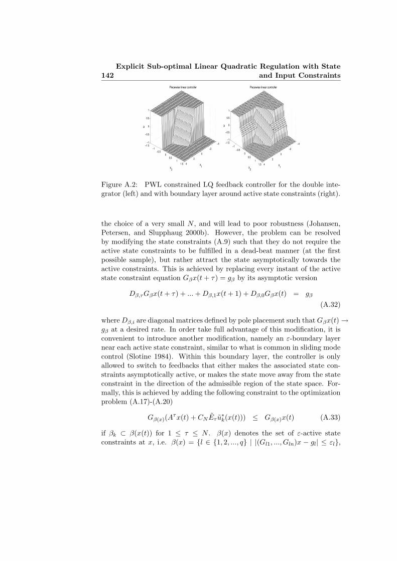
142Explicit Sub-optimal Linear Quadratic Regulation with State
and Input Constraints
−4
−2
0
2
4
−1.5−1
−0.50
0.51
1.5
−1
−0.5
0
0.5
1
x1
Piecewise linear controller
x2
u−4
−2
0
2
4
−1.5−1
−0.50
0.51
1.5
−1
−0.5
0
0.5
1
x1
Piecewise linear controller
x2
u
Figure A.2: PWL constrained LQ feedback controller for the double inte-grator (left) and with boundary layer around active state constraints (right).
the choice of a very small N , and will lead to poor robustness (Johansen,Petersen, and Slupphaug 2000b). However, the problem can be resolvedby modifying the state constraints (A.9) such that they do not require theactive state constraints to be fulfilled in a dead-beat manner (at the firstpossible sample), but rather attract the state asymptotically towards theactive constraints. This is achieved by replacing every instant of the activestate constraint equation Gβx(t + τ) = gβ by its asymptotic version
Dβ,τGβx(t + τ) + ... + Dβ,1x(t + 1) + Dβ,0Gβx(t) = gβ
(A.32)
where Dβ,i are diagonal matrices defined by pole placement such that Gβx(t) →gβ at a desired rate. In order take full advantage of this modification, it isconvenient to introduce another modification, namely an ε-boundary layernear each active state constraint, similar to what is common in sliding modecontrol (Slotine 1984). Within this boundary layer, the controller is onlyallowed to switch to feedbacks that either makes the associated state con-straints asymptotically active, or makes the state move away from the stateconstraint in the direction of the admissible region of the state space. For-mally, this is achieved by adding the following constraint to the optimizationproblem (A.17)-(A.20)
Gβ(x)(Aτx(t) + CN Eτ u
∗k(x(t))) ≤ Gβ(x)x(t) (A.33)
if βk ⊂ β(x(t)) for 1 ≤ τ ≤ N . β(x) denotes the set of ε-active stateconstraints at x, i.e. β(x) = {l ∈ {1, 2, ..., q} | |(Gl1, ..., Gln)x − gl| ≤ εl},

A.4 State space partitioning 143
where εl > 0 defines the boundary layer. Eq. (A.33) excludes non-attractivefeedbacks that tend to move the state towards violation of active state con-straints.
Double integrator example, cont’d. In order to reduce the gainnear the active state constraints, a boundary layer of ε1 = ε2 = ±0.15is defined around the constraints x2 = 0.5 and x2 = −0.5. Hence, when0.65 ≥ x2 ≥ 0.35, the control strategy is allowed to switch and the controllertakes the objective of attracting the state towards the surface x2 = 0.5 whileminimizing the LQ objective. The speed of the motion towards the surfacex2 = 0.5 is defined by D1 = 1/0.9 and D2 = 1. Comparing the piecewiselinear controller surface of the modified controller (right part of Figure A.2)with the original controller (left part of Figure A.2), it is seen that the gainhas indeed been reduced in an ε-boundary layer near the active constraintsx2 = ±0.5. �
A.4 State space partitioning
The purpose of this section is to discuss how to solve the outer optimizationproblem (A.17)-(A.20), and in particular to derive an algorithm for com-puting a state space partitioning that can be used to decide which activeconstraint set sequence is optimal at a given state. The discrete minimiza-tions in (A.17) and (A.23) can either be avoided completely in the real-timecomputations if the set of candidate optima is reduced to single elementswithin subsets of the state space, or at least reduced to a small subset ofC within subsets of the state space. This can be exploited in the real-timeimplementation to reduce the processing capacity and memory requirementsand also for computational analysis as considered in section A.5.
A.4.1 Activity region
The activity region Xk ⊂ X is defined as the subset of the state space wherethe active constraint set sequence with index k is active, i.e. Xk = {x ∈X | k = k∗(x)}. Together with the affine functions (A.30), the activityregions Xk, k ∈ C completely describes the PWL structure of the controller.
Double integrator example, activity regions. For the double inte-grator example, there are five constituent affine feedbacks with correspond-ing activity regions. Region/Feedback 0: unconstrained case (k = 0), Re-gion/Feedback 1: input constraint u = −1 active (k = 1), Region/Feedback2: input constraint u = 1 active (k = 2), Region/Feedback 3: state con-straint x2 = −0.5 active (k = 3), Region/Feedback 4: state constraint

144Explicit Sub-optimal Linear Quadratic Regulation with State
and Input Constraints
x2 = 0.5 active (k = 4). The activity regions for the suboptimal constrainedLQ controller with boundary layer are shown in Figure A.3. We observethat in this case the regions can be characterized as unions of polyhedra. �
−4 −3 −2 −1 0 1 2 3 4−1.5
−1
−0.5
0
0.5
1
1.5Activity sets
x1
x 2 Feedback 0
Feedback 1
Feedback 2
Feedback 3
Feedback 4
Figure A.3: Activity regions for the five constituent affine feedbacks in theconstrained LQR for the double integrator with boundary layers.
In order to explicitly characterize the activity regions, it is natural totreat the feasible and relaxed feasible regions XF and XR separately, sincethe choice of optimal active constraint set sequence is based on differentcriteria in these cases. Thus, we define the activity regions contained in XF
as follows:
Xfk = {x ∈ XF
k | k is optimal w.r.t. (A.17) − (A.20) and (A.33)}(A.34)
For x ∈ XR, the controller objective changes to minimize the constraintviolation and we define
Xrk =
{x ∈ XR
k | k is optimal w.r.t. (A.23) − (A.25)}
(A.35)
Hence, the activity region Xk where the feedback with index k is active isnow Xk = Xf
k ∪ Xrk . A slightly more explicit characterization of Xf
k than(A.34) is
Xfk =
{x ∈ XF
k | ϕk(x) ≤ ϕj(x), j ∈ F(x) ∩ A(x)}
(A.36)

A.4 State space partitioning 145
where F(x) = {k ∈ C | (x) ∈ XFk } is a set containing the active constraint set
sequences that are feasible at x, and A(x) ⊂ C is a set containing the indicesto the active constraint set sequences that are attractive or not currentlyactive at x, cf. (A.33):
A(x) ={
k ∈ C | Gβ(x)(Aτx + CN Eτ u
∗k(x)) ≤ Gβ(x)x
or βk 6⊂ β(x)} (A.37)
Furthermore, it follows that
XF =⋃
k∈C
Xfk =
⋃
k∈C
XFk (A.38)
Likewise, a slightly more explicit characterization of Xrk than (A.35) is given
by
Xrk =
{x ∈ XR
k | νk(x) ≤ νj(x), for all j ∈ R(x)}
(A.39)
where R(x) = {k ∈ C | x ∈ XRk } is defined as the set of active constraint
set sequences that are feasible with respect to the non-relaxable constraints,but not feasible with respect to the relaxable constraints at x. We also have
XR =⋃
k∈C
Xrk =
⋃
k∈C
XRk (A.40)
which is the set of states where there exists an active constraint set sequencethat is feasible and optimal with respect to the non-relaxable constraints butnot with respect to the relaxable constraints.
A.4.2 Outer Approximations to the Activity Regions
Since XFk and XR
k are polyhedral, it is clear that XF , XR and X = XF ∪XR
are unions of polyhedra. However, because the optimality conditions in(A.36) are characterized by quadratic functions, the set Xk ⊂ X may not becharacterized only by the hyper-planes defined by feasibility, but possiblyalso by other hyper-planes or (convex or non-convex) quadratic surfaces dueto the optimality conditions. Thus, Xk may in general not be a union ofpolyhedra and therefore difficult to characterize exactly in a more explicitmanner than (A.36) and (A.39). Still, several explicit outer approximationsof Xk can be computed in terms of sets that contain Xk. Here we developan outer approximation Xk ⊃ Xk where Xk is a union of polyhedra. Asthe basic polyhedral building blocks in this characterization we consider the

146Explicit Sub-optimal Linear Quadratic Regulation with State
and Input Constraints
hyperplane partition PHPX = {XHP
l | l ∈ {1, 2, ..., NP }} generated by all thehyper-planes involved in the characterization of XF
k , XRk and XA
k , for k ∈ C:
HEτKk,2x = h − HEτ (Kgk,1g + Kh
1,kh)
(A.41)
G(Aτ + CN EτKk,2)x = g − GCN Eτ (Kgk,1g + Kh
k,1h)
(A.42)
G(Aτ + CN EτK2,k − I)x = GCN Eτ (Kh1,kh + Kg
1,kg)
(A.43)
for 1 ≤ τ ≤ N , with obvious interpretation when h or g are zero-dimensional.Let (A.41)-(A.43) be written in compact notation Y x = y. The set of half-spaces Y+
i = {x ∈ Rn | Yix ≥ yi} and Y−i = {z ∈ Rn | Yix < yi} now
defines the hyperplane partition PHPX of X as the set of all possible non-
empty intersections of half-spaces: XHPl = Y∗
1 ∩ ...∩Y∗Nz
where ∗ symbolizesany combinations of +/−. Note that this hyperplane partition will containunnecessarily many elements in many cases and is introduced here in orderto develop a theoretical understanding.
Lemma 2 The hyperplane partition PHPX has the following properties:
i. Each constituent region of the partition is uniquely associated witheither the feasible region XF or the relaxed feasible region XR, i.e.XHP
l ∩ XF = ∅ and XHPl ∩ XR = XHP
l , or vice versa XHPl ∩ XF =
XHPl and XHP
l ∩ XR = ∅, for all l = 1, 2, ...., NP .
ii. For all l ∈ {1, 2, ..., Np} and x ∈ XHPl the sets F(x), R(x), A(x) and
β(x) are invariant such that each of them contain the same elementsfor all x ∈ XHP
l .
Proof. Follows from the fact that the hyperplane partition PHPX of X
is generated by all hyper-planes involved in the characterizations of F(x),R(x), A(x) and β(x). �
From the first part of Lemma 2 it is evident that each XHPl ∈ PHP
X isfully contained in either XR or XF . Thus, we define disjoint index sets
LF ={l ∈ {1, 2, ..., NP } | XHP
l ∩ XF 6= ∅}
(A.44)
LR ={l ∈ {1, 2, ..., NP } | XHP
l ∩ XR 6= ∅}
(A.45)
Assume l ∈ LF , i.e. XHPl ⊂ XF . One may now define a set Ff
l {k ∈C | XHP
l ∩ XFk 6= ∅} of feasible active constraint set sequences in the region

A.4 State space partitioning 147
XHPl . Hence, for any x ∈ XF there exists a unique l(x) ∈ LF such that
x ∈ XFl(x) and at least one of the feasible active constraint set sequences in
Ffl is optimal for all x ∈ XHP
l . We continue by characterizing the subset
of Ffl that is optimal for some x ∈ X F
l , aiming towards a definition of
Xfk ⊃ Xf
k .
Lemma 3 Let l ∈ LF and j, k ∈ Ffl be arbitrary. Suppose the active con-
straint set sequences ((αk1 , β
k1 ), (αk
2 , βk2 ),..., (αk
NS, βk
NS)) and ((αj
1, βj1),
(αj2, β
j2), ..., (α
jNS
, βjNS
)) are different. If αki ⊂ αj
i and βki ⊂ βj
i , for alli = 1, 2, ..., NS, then the active constraint set sequence with index j is sub-optimal for all x ∈ XHP
l .
Proof. Because the active constraint set sequence with index k is a sub-set of the active constraint set sequence with index j and both are feasible,it follows immediately that ϕk(x) ≤ ϕj(x) for all x ∈ XHP
l since adding aconstraint to some constraint set sequence will not reduce the cost. �
Lemma 4 Let l ∈ LF and k ∈ Ffl be arbitrary, and define
γjk = maxx∈XHP
l
(ϕk(x) − ϕj(x)) (A.46)
κjk = minx∈XHP
l
(ϕk(x) − ϕj(x)) (A.47)
If γjk ≤ 0 for all j ∈ Ffl , then the active constraint set sequence with index
k is optimal for all x ∈ XHPl . If κjk ≥ 0 for all j ∈ Ff
l , then the activeconstraint set sequence with index k is suboptimal for all x ∈ XHP
l .
Proof. Since γjk ≤ 0 it follows that for all x ∈ XHPl and j ∈ Ff
l ,
ϕk(x) ≤ ϕj(x). Note that due to Lemma 2, F fl = F(x) for all x ∈ XHP
l ,
and the first part follows because F fl contains all feasible active constraint
set sequences in C. The second part of the lemma is analogous. �
Both (A.46) and (A.47) are quadratic programs, for a fixed l ∈ LF and
fixed active constraint set sequences k, j ∈ F fl , since XHP
l is polyhedraland ϕk and ϕj are quadratic. Using the optimality characterizations inLemmas 3 and 4, one will typically be able to exclude a large set of candidateactive constraint set sequences from the set of feasible active constraint setsequences Ff
l in the region XHPl . We define Of
l ⊂ FFl as the indices of

148Explicit Sub-optimal Linear Quadratic Regulation with State
and Input Constraints
those active constraint set sequences that are consistent with the optimalityconditions in Lemmas 3 and 4 in XHP
l :
Ofl =
{
k ∈ Ffl | k is optimal w.r.t. (A.17)-(A.20), (A.33)
for some x ∈ XHPl
}(A.48)
We define the outer approximation to the activity region Xfk as follows:
Xfk =
⋃
l∈LF
XHPl (A.49)
Next, assume l ∈ LR, i.e. XHPl ⊂ XR. One may now define a set F r
l = {k ∈C | XHP
l ∩XRk 6= ∅} of relaxed feasible active constraint set sequences in the
region XHPl . Unlike the characterization of Xf
k , we now have the followingresult:
Lemma 5 For all k ∈ C, the set Xrk is a union of polyhedra.
Proof. Let k ∈ C be arbitrary. The region of relaxed feasibility XRk is
polyhedral, cf. (A.27). Since the function νk(x)−νj(x) is piecewise linear inx, the sets {x ∈ Rn | νk(x) ≤ νj(x)} that appear in the optimality conditionin (A.39) are characterized using hyper-planes. Since all geometric objectscharacterizing Xr
k are hyper-planes, it is a union of polyhedral sets. �
According to Lemma 5 it is possible to obtain an exact and explicitcharacterization of Xr
k . However, for computational reasons it may be con-venient with an outer approximation X
rk ⊃ Xr
k in some cases. The followingoptimality lemma is useful in that respect:
Lemma 6 Let l ∈ LR and k ∈ Frl be arbitrary, and define
ρjk = maxx∈XHP
l
(νk(x) − νj(x)) (A.50)
σjk = min(x)∈XHP
l
(νk(x) − νj(x)) (A.51)
If ρjk ≤ 0 for all j ∈ F rl , then the active constraint set sequence with index
k is optimal for all x ∈ XHPl . If σjk ≥ 0 for all j ∈ FR
l , then the activeconstraint set sequence with index k is suboptimal for all x ∈ XHP
l .
Proof. Analogous to Lemma 4. �

A.4 State space partitioning 149
Note that (A.50) and (A.51) are piecewise linear programs. Using theoptimality characterizations in Lemma 6, one will typically be able to ex-clude a large set of candidate active constraint set sequences from the setof feasible active constraint set sequences F r
l in the region XHPl . We define
Orl ⊂ FR
l as the indices of those active constraint set sequences that areconsistent with the optimality conditions of Lemma 6 in XHP
l :
Orl = {k ∈ Fr
l | k is optimal w.r.t. (A.23)-(A.25)
for some x ∈ XHPl
}(A.52)
Finally, we define the outer approximation to the activity region Xrk as
follows:
Xrk =
⋃
l∈LR
XHPl (A.53)
We are now in position to define Xk = Xfk ∪ X
rk and
Fl =
{
Ffl , l ∈ LF
Frl , l ∈ LR , Ol =
{
Ofl , l ∈ LF
Orl , l ∈ LR (A.54)
A.4.3 Partitioning Algorithm
Algorithm 1
i. Let E := ∅, and U := {X}.
ii. If U = ∅, the partition generated by this algorithm is P = E and thealgorithm terminates.
iii. Let X0 ∈ U be arbitrary.
iv. Let O0 contain the candidate optimal active constraint set sequencesin X0, computed according to Lemmas 3-6.
v. If O0 contains a sufficiently small number of elements, add X0 to theset of explored subsets E and remove X0 from the set of unexploredsubsets U . Go to step 2.
vi. Select a hyperplane Yix = yi from Y x = y and split X0 into non-empty X+
0 = X0 ∩ Y+i and X−
0 = X0 ∩ Y−i . If this is not possible for
any hyperplane from Y x = y, add X0 to the set of explored subsets Eand remove X0 from the set of unexplored subsets U . Go to step 2.

150Explicit Sub-optimal Linear Quadratic Regulation with State
and Input Constraints
vii. Add X+0 and X−
0 to U and remove X0 from U . Go to step 2.
The set E contains the set of explored subsets of X, while the set U containsthe set of explored subsets of X. The algorithm will explore the candidateoptimal active constraint sets associated with each element of E sequen-tially. The regions of X will be split using the hyper-planes from Y x = yand explored individually until either a sufficiently small number of can-didate optimal active constraint set remains in each region, or the regioncan not be split any further using hyper-planes from Y x = y. In order toreduce the computational complexity of Algorithm 1 one should implementheuristics in step 6 in order to select a ”promising” hyperplane for splittingthe region X0 such that unnecessary splitting is avoided. Note that the par-tition PX generated by Algorithm 1 may be unnecessarily fine since at eachstep it is not known a priori if one can reduce the number of elements inO0 by further partitioning of X0. Hence, after the algorithm terminates, thenumber of constituent polyhedra in the partition of X can often be reducedconsiderably by aggregating pairs of neighboring polyhedra whenever theirunion remains polyhedral, see also (Bemporad, Fukuda, and Torrisi 2001).
−4 −2 0 2 4−1.5
−1
−0.5
0
0.5
1
1.5
R1
R2
R3
R4
R5
R6
R7
R8R9
R10
R11
x1
x 2
Figure A.4: Partition for the constrained LQR for the double integratorwith boundary layers.
Double integrator example, cont’d. The partition computed usingAlgorithm 1 with a successive aggregation of neighboring regions is shownin Figure A.4. We observe that the number of regions is 11, which is the

A.5 Optimality, complexity and real-time implementation 151
smallest possible number of polyhedral regions capable of characterizing theactivity sets for this problem. Also, we observe that within each region,there is a single candidate optimal active constraint set sequence. Hence,the PWL feedback law is explicitly characterized by this partition. Feedback0 (unconstrained case) is associated with R1, R3 and R4 in this partition.Feedback 1 (u = −1) is associated with R5 and R11. Feedback 2 (u = 1) isassociated with R7 and R10. Feedback 3 (x2 = −0.5) is associated with R2and R6, while feedback 4 (x2 = 0.5) is associated with R8 and R9. �
A.5 Optimality, complexity and real-time imple-mentation
A.5.1 Upper and lower bounds on cost function
Define the closed loop performance of the suboptimal constrained LQR asfollows:
V (x(0)) =
∞∑
t=0
(xT (t)Qx(t) + (u∗(t))T Ru∗(t)
)(A.55)
For example 1, upper and lower bound on cost V (x(0)) are illustrated inFigure A.5. These bounds are computed by solving LMIs with a continuouspiecewise quadratic parameterization of the functions as described in (Jo-hansson and Rantzer 1998; Rantzer and Johansson 2000), see (Johansen,Petersen, and Slupphaug 2000b) for details. Note that a continuous-timeapproximation is utilized due to restrictions in the available software im-plementation (Hedlund and Johansson 1999), and that the bounds have nodirect meaning for x 6∈ XF , except that the upper bound defines a Lyapunovfunction (under a detectability assumption).
A.5.2 Complexity reduction by sub-optimality
It was claimed initially that we expect that the restrictions introduced onthe allowed active constraint set sequence switching times will reduce thecomputational complexity of the controller, i.e. lead to a partition of thestate space with less regions. We illustrate this by an example.
Example 2, Double integrator (Bemporad, Morari, Dua, andPistikopoulos 2002). Consider the double integrator
A =
(1 Ts
0 1
)
, B =
(T 2
s
Ts
)
(A.56)

152Explicit Sub-optimal Linear Quadratic Regulation with State
and Input Constraints
−4−2
02
4 −2−1
01
20
50
100
150
x2
Upper and lower bounds on cost
x1
Figure A.5: Upper and lower bounds on the cost for the constrained LQRfor the double integrator with boundary layers.
with sampling-interval Ts = 0.05. The control objective is defined by thecost function lQR(x, u) = x2
1 + 0.1u2 and the constraints −1 ≤ u ≤ 1. Weconsider two cases
i. N = 8, with no restrictions on the number of active constraint setswitches on the horizon, same as (Bemporad, Morari, Dua, and Pis-tikopoulos 2002).
ii. N = 8, S = 2, N2 = 3, i.e. only one active constraint set switchallowed on the horizon
The second case leads to the following nine candidate active constraintset sequences that enumerates the set C:
First 3 samples Last 5 samples
u = Kx u = Kxu = Kx u = −1u = Kx u = 1u = −1 u = Kxu = −1 u = −1u = −1 u = 1u = 1 u = Kxu = 1 u = −1u = 1 u = 1

A.5 Optimality, complexity and real-time implementation 153
The suboptimal strategy gives a reduction from 93 to 33 regions, whichallows a significant reduction of the real-time processing and memory re-quirements. From Figure A.6 we observe that the differences in the closedloop trajectories for x(0) = (−3, 3)T are not very significant. �
−3 −2 −1 0 1 2 3−2
−1
0
1
2
3
4
x1
x 2
optimal trajectory
suboptimal trajectory
Figure A.6: Example of trajectories with and without active constraint setchange restrictions.
A.5.3 Real-time Implementation
The suboptimal constrained LQR is a PWL function of the state. However,efficient evaluation of this PWL function in the real-time control systemrequires that one is able to efficiently compute in real time which affinefeedback to associate with each vector x. The affine state feedbacks arecomputed offline and stored in real-time computer memory. Whether it isdesirable to also compute offline an explicit characterization of the subsetsof X where each affine feedback is active depends on several factors: Ac-ceptable offline processing time, available real-time computer memory andreal-time computer processing capacity. There exist at least two real-timeimplementation strategies that can be employed in order to address theabove mentioned tradeoffs:
i. The discrete optimization problems (A.17)-(A.20) and (A.23)-(A.25)are solved in real time. Discrete search techniques such as branch-and-bound and A∗ can be applied for this purpose (Korf 1990).
ii. A partitioning of X such that within each constituent region of the

154Explicit Sub-optimal Linear Quadratic Regulation with State
and Input Constraints
−4 −3 −2 −1 0 1 2 3 4−4
−3
−2
−1
0
1
2
3
4
R1
R2
R3
R4
R5
R6
R7
R8
R9
x 2
−4 −3 −2 −1 0 1 2 3 4−4
−3
−2
−1
0
1
2
3
4
R1
R2
R3
Figure A.7: Double integrator with input constraints and N = 8. Top:Simple partition where the maximum number of candidate state feedbacksin each region is 3. Bottom: Simple partition where the maximum numberof candidate state feedbacks in each region is 5.
partition there are at most a given small number of affine feedbacksthat may be optimal. A search among the small number of remainingcandidates (if more than one) is then carried out in real time.
Example 2, continued. By early termination of the partitioning algo-rithm one can achieve for example the partitions shown in Figure A.7. Inthe first case there are 9 regions, each with a list of up to 3 affine feedbacksthat are optimal at various states within each region, see Table A.1. In thesecond case there are 3 regions, with a list of up to 5 affine feedbacks thatare optimal at various states in each region, see also Table A.1. Hence, onecan reduce the complexity of the partition by comparing the values of a user-specified number of quadratic functions and linear constraints in real time.

A.5 Optimality, complexity and real-time implementation 155
In a sense, one has a method for partially solving the real-time quadraticprogram offline. �
Region Candidate optimal feedbacks
9 regions R1 {1}R2 {3, 6, 9}R3 {2, 5, 8}R4 {7, 8, 9}R5 {9}R6 {2, 8, 9}R7 {4, 5, 6}R8 {3, 5, 6}R9 {5}
3 regions R1 {1, 4, 5, 7, 9}R2 {3, 5, 6, 9}R3 {2, 5, 8, 9}
Table A.1: List of candidate optimal feedbacks for the simplified partitionsof example 2.
Example 3, laboratory model helicopter. A laboratory model he-licopter (Quanser 3-DOF Helicopter) with two DC-motor driven rotors issampled with T = 0.01s, and the following state-space representation isobtained
A =
1 0 0.01 0 0 00 1 0 0.01 0 00 0 1 0 0 00 0 0 1 0 0
0.01 0 0 0 1 00 0.01 0 0 0 1
, B =
0 00.0001 −0.00010.0019 0.00190.0132 −0.0132
0 00 0
The states of the system are x1 - elevation, x2 - pitch angle, x3 - elevationrate, x4 - pitch angle rate, x5 - integral of elevation error, and x6 - integralof pitch angle error. The inputs are u1 and u2, the front and rear rotorvoltages. Assume the system is to be regulated to some setpoint with thefollowing constraints on the inputs, pitch and elevation rates −1 ≤ u1 ≤ 3,−1 ≤ u2 ≤ 3, −0.25 ≤ x3 ≤ 0.25, and −0.6 ≤ x4 ≤ 0.6. The LQ costfunction is given by Q = diag(100, 20, 40, 8, 1, 0.5) and R = diag(1, 1). WithN = 1 this leads to 33 active constraint sets. Comparing their quadratic
156Explicit Sub-optimal Linear Quadratic Regulation with State
and Input Constraints
cost function and evaluating the linear constraints requires in the worst case320 microseconds on a 450 MHz Pentium II with our implementation. Ifnecessary, this can be reduced by state space partitioning using Algorithm1. The experimental results in Figure A.8 compares the performance alongthe elevation axis with unconstrained LQR. �
Another experimental case study utilizing this approach in an automo-tive application is reported in (Petersen, Johansen, Kalkkuhl, and Ludemann2001). Due to the exponential growth of the number of candidate activeconstraint set sequences as the number of states, horizon and constraintsincreases, the approach is restricted to problems of low and moderate com-plexity. As the problem complexity increases, the use of prior knowledge andsimulation are the keys to restricting the number of candidate active con-straint set sequences and the (offline and online) computational complexity.
A.6 Conclusions
A suboptimal strategy for explicit offline design of LQ controllers subject tostate and input constraints is derived. It is demonstrated that allowing sub-optimality in terms of restrictions on the number of allowed active constraintset changes on the horizon leads to significant reduction in the complexity ofthe state space partitioning. The method gives the user flexibility to addressthe tradeoff between real-time computer memory and processing capacity.

A.6 Conclusions 157
0 10 20 30 40 50 60 70−0.5
−0.4
−0.3
−0.2
−0.1
0
0.1
0.2
0.3
0.4
0.5
time (s)
Eleva
tion (
m)
Elevation with unconstrained LQR
0 10 20 30 40 50 60 70−0.5
−0.4
−0.3
−0.2
−0.1
0
0.1
0.2
0.3
0.4
0.5
time (s)
Eleva
tion (
m)
Elevation with constrained LQR
0 10 20 30 40 50 60 70−0.8
−0.6
−0.4
−0.2
0
0.2
0.4
0.6
0.8
time (s)
Eleva
tion r
ate (m
/s)
Elevation rate with unconstrained LQR
0 10 20 30 40 50 60 70−0.4
−0.3
−0.2
−0.1
0
0.1
0.2
0.3
0.4
time (s)
Eleva
tion r
ate (m
/s)
Elevation rate with constrained LQR
Figure A.8: Experimental results with 3-DOF laboratory model helicopter.

158Explicit Sub-optimal Linear Quadratic Regulation with State
and Input Constraints

Appendix B
Details of Proof
In this section it is proven that (4.37) implies D(v) > 0 for all v > 0.
P1,1(v) =∂P1,1(v)
∂vv =
(
α21 + β2
1R−1
(
Q2,2(v) +2(Q1,1(v)/R−1)
1/2
β1v
))1/2ddvQ1,1(v)
2β1 (Q1,1(v)R−1)1/2v
+
(Q1,1(v)R−1
)1/2β1
(
ddvQ2,2(v) +
2(Q1,1(v)/R−1)1/2
β1+
ddv
Q1,1(v)
β1(Q1,1(v)R−1)1/2 v
)
2
(
α21 + β2
1R−1
(
Q2,2(v) +2(Q1,1(v)/R−1)1/2
β1v
))1/2v
(B.1)
P1,2(v) = P2,1(v) =∂P1,2(v)
∂vv =
((Q1,1(v)/R−1
)1/2
β1+
ddvQ1,1(v)
2β1 (Q1,1(v)R−1)1/2v
)
v (B.2)
P2,2(v) =
α1 +
(
α21 + β2
1R−1
(
Q2,2(v) +2(Q1,1(v)/R−1)
1/2
β1v
))1/2
β21R−1
v
+
(
ddvQ2,2(v) +
2(Q1,1(v)/R−1)1/2
β1+
ddv
Q1,1(v)
β1(Q1,1(v)R−1)1/2 v
)
v
2
(
α21 + β2
1R−1
(
Q2,2(v) +2(Q1,1(v)/R−1)1/2
β1v
))1/2v (B.3)

160 Details of Proof
Now
D(v) =
(
α21 + β2
1R−1
(
Q2,2(v) +2(Q1,1(v)/R−1)
1/2
β1v
))1/2ddvQ1,1(v)α1
2β1 (Q1,1(v)R−1)1/2 β21R−1
+
(
α21 + β2
1R−1
(
Q2,2(v) +2(Q1,1(v)/R−1)
1/2
β1v
))
ddvQ1,1(v)
2β1 (Q1,1(v)R−1)1/2 β21R−1
+
ddvQ1,1(v)
(
ddvQ2,2(v) +
2(Q1,1(v)/R−1)1/2
β1+
ddv
Q1,1(v)
β1(Q1,1(v)R−1)1/2 v
)
v
4β1 (Q1,1(v)R−1)1/2
+
(Q1,1(v)R−1
)1/2β1
(
ddvQ2,2(v) +
2(Q1,1(v)/R−1)1/2
β1+
ddv
Q1,1(v)
β1(Q1,1(v)R−1)1/2 v
)
2
(
α21 + β2
1R−1
(
Q2,2(v) +2(Q1,1(v)/R−1)1/2
β1v
))1/2
α1
β21R−1
+
(Q1,1(v)R−1
)1/2β1
(
ddvQ2,2(v) +
2(Q1,1(v)/R−1)1/2
β1+
ddv
Q1,1(v)
β1(Q1,1(v)R−1)1/2 v
)
2β21R−1
+
(Q1,1(v)R−1
)1/2β1
(
ddvQ2,2(v) +
2(Q1,1(v)/R−1)1/2
β1+
ddv
Q1,1(v)
β1(Q1,1(v)R−1)1/2 v
)2
4
(
α21 + β2
1R−1
(
Q2,2(v) +2(Q1,1(v)/R−1)1/2
β1v
)) v
−((
Q1,1(v)/R−1)1/2
β1+
ddvQ1,1(v)
2β1 (Q1,1(v)R−1)1/2v
)2
Define the following positive variables:
A = α21 + D
(
Q2,2(v) +2C
Dv
)
= α21 + DQ2,2(v) + 2Cv
B =d
dvQ2,2(v) +
2C
D+
ddvQ1,1(v)
Cv
C =(Q1,1(v)R−1
)1/2β1
D = β21R−1

Details of Proof 161
The above expression can then be rewritten to
D(v) =A1/2 d
dvQ1,1(v)α1
2CD+
A ddvQ1,1(v)
2CD+
ddvQ1,1(v)Bv
4C
+α1BC
2A1/2D+
CB
2D+
CB2
4Av −
(
C
D+
ddvQ1,1(v)
2Cv
)2
(B.4)
In (B.4) there are two possible negative factors involved: α1 and the lastquadratic term with a negative sign (−P
′
1,2(v)P′
2,1(v)). To cancel P′
1,2(v)P′
2,1(v),parts from the 3rd and 5th term in (B.4) are used which gives
ddvQ1,1(v)Bv
4C+
CB
2D−(
C
D+
ddvQ1,1(v)
2Cv
)2
=ddvQ2,2(v) d
dvQ1,1(v)
4Cv
+d
dvQ2,2(v)
The following inequality thus ensures D(v) > 0:
D(v) =A1/2 d
dvQ1,1(v)α1
2CD+
A ddvQ1,1(v)
2CD+
ddvQ2,2(v) d
dvQ1,1(v)
4Cv
+α1BC
2A1/2D+
d
dvQ2,2(v) +
CB2
4A> 0 (B.5)
where only α1 may have a negative value.

162 Details of Proof