2014 - university of baghdad amin 001/journey/2014...abeer hussein al-shammari 15 ? 27 ... 77...
TRANSCRIPT

June
2014 Number 6
Volume 20

6العدد
02المجلد
حزيران
0224

College of Engineering University of Baghdad
List of Contents
English Section: Page Assessment of Modified - Asphalt Cement Properties
Prof. Saad Isa Sarsam
Ibtihal Mouiad Lafta
1 - 14
Finite Element Analysis of Reinforced Concrete T-Beams with Multiple Web
Openings under Impact Loading
Prof. Dr. Nazar Kamel Oukaili
Abeer Hussein Al-Shammari
15 ? 27
Performance Analysis of Four Conceptual Designs for the Air Based Photovoltaic /
Thermal Collectors
Karima Esmail Amori
Mustafa Adil Al-Damook
28 ? 45
Modeling of Electron and Lattice Temperature Distribution Through Lifetime of
Plasma Plume
Ali Hamza Alwan Al-taee
46 ? 62
Energy Savings in Thermal Insulations for Sustainable Buildings Prof.Dr. Angham Alsaffar
Qusay Adnan Alwan
63 ? 77
Studying the Effects of Contamination on Soil Properties using Remote Sensing Dr. Mahdi O. Karkush
Dr.Abdul Razak T .Ziboon
Hadeel M. Hussien
78 ? 90
The Effect of Ceramic Coating on Performance and Emission of Diesel Engine
Operated on Diesel Fuel and Biodiesel Blends
Dr. Ibtihal Al-Namie
Dr. Mahmoud A. Mashkour
Ali Abu Al-heel Qasim
91 ? 108
Compression of an ECG Signal sing Mixed Transforms
Sadiq Jassim Abou-Loukh
Jaleel Sadoon Jameel
109 ? 123
Study the Effect of Face Sheets Material on Strength of Sandwich Plates with
Circular Hole.
Dr. Hatem Rahem Wasmi
Nawal Falkhous Eshaut
124 ? 142
Kinetics of the Saponification of Mixed Fats Consisting of Olein and Stearin Dr. Raghad Fareed Kassim Almilly
143 ? 159
Analysis and Control of PWM Buck-Boost AC Chopper Fed Single-Phase
Capacitor Run Induction Motor Prof. Dr. Jafar H. Alwash
Asst. Prof. Dr. Turki K. Hassan
Shams W. Kamel
160- 178

Numerical Study of Optimum Configuration of Unconventional Airfoil with
Steps and Rotating Cylinder for Best Aerodynamics Performance Dr. Najdat N. Abdulla
Ahmed J. Hamoud
179 ? 199
Journal of Engineering Volume 20 June - 2014 Number 6
1
Assessment of Modified - Asphalt Cement Properties
Prof. Saad Issa Sarsam Ibtihal Mouiad Lafta
Department of Civil Engineering Department of Civil Engineering
College of Engineering College of Engineering
University of Baghdad University of Baghdad
ABSTRACT
The Asphalt cement is produced as a by-product from the oil industry; the asphalt
must practice further processing to control the percentage of its different ingredients so that it
will be suitable for paving process. The objective of this work is to prepare different types of
modified Asphalt cement using locally available additives, and subjecting the prepared
modified Asphalt cement to testing procedures usually adopted for Asphalt cement, and
compare the test results with the specification requirements for the modified Asphalt cement
to fulfill the paving process requirements. An attempt was made to prepare the modified
Asphalt cement for pavement construction in the laboratory by digesting each of the two
penetration grade Asphalt cement (40-50 and 60-70) with sulfur, fly ash, silica fumes. Three
different percentages of each of the above mentioned additives have been tried using
continuous stirring and heating at 150 ºC for 30 minutes .
The prepared modified Asphalt specimens were subjected to physical properties
determination; the penetration, softening point, ductility before and after laboratory aging. It
was concluded that all percentage of additives has reduced the penetration value of asphalt
cement, an exception to that could be noticed when using asphalt cement (40-50) and when
adding sulfur. Softening point was increased with the addition of all percentage of additives
except that with 7% sulfur by wt. of asphalt cement (40-50) it decreased by 8%.
After aging in general, the penetration decreased by about 37% for control specimens and the
softening point increased by about 8% for control specimens.
For asphalt cement 40-50 after aging, Sulfur has the least impact on ductility since it reduces
it by 20%. Silica fumes have moderate effect on ductility when it reduces it by 35%, while fly
ash shows the highest impact of 36%. For asphalt cement 60-70 after aging, sulfur was able to almost retain its ductility, while fly
ash shows moderate reduction in ductility within a range of 20-36% and silica fumes shows
high impact on ductility in the range of 30-50%.
Keywords: Ductility, Fly ash, Silica Fumes, Modified asphalt cement, sulfur, softening
point, penetration.

Journal of Engineering Volume 20 June - 2014 Number 6
2
دراسة لخصائص االسفلث االسمنتي المحسن
أ. سعذ عيسى سرسم ابتهال مؤيذ لفتة
قسم الهنذسة المذنية قسم الهنذسة المذنية
جامعة بغذاد كلية الهنذسة / جامعة بغذاد كلية الهنذسة /
الخالصة
خى إخبج االسفهج انسخ كخح ثبي ي قبم صبػت انفط، دب ا خضغ نهؼذذ ي انؼهبث ي اخم انسطشة ػهى انسب
نخخهفت بحث حك يبسبت نؼهت انشصف.انذف ي زا انؼم إػذاد أاع يخخهفت ي االسفهج انسخ ي يكبح ا انئ
بزنج يحبالث .حؼذهب ببسخخذاو انضبفبث انخفشة يحهب، إخضبع االسفهج انسخ انؼذل نؼذذ ي إخشاءاث االخخببس
( يغ 04-04 04-04ث حى اسخخذاو ػ ي االسفهج انسخ ر اخخشاق دسخت )نخحضش االسفهج انسخ انؼذل ف انخخبش ح
(.حى اسخخذاو ثالثت سب يخخهفت ي كم ي اناد انضبفت انزكسة أػال غببس انسهكب انضبفبث )انكبشج ,انشيبد انخطبش
انفحصبث نخحذذ .نؼذذ ية صف سبػت. اخشج ايئت نذ 004نهخهط يغ انخسخ بذسخت خضؼج ػبث األسفهج انؼذل
قبم بؼذ انخقبدو انخخبشي . بانخصبئص انفضبئت؛. اخخشاق، قطت انهت،انقذس ػهى انسح
بؼذ اضبفت انكبشج بب 04-04حى االسخخبج بب انضبفبث قبيج بخقهم قى االخخشاق بصسة ػبيت ببسخثبء االسفهج انسخ ع
نالسفهج ري % 8% حث قهج بقذاس 0ادث دسخت حشاسة انهت ػذ اسخخذاو انضبفبث يغ اسخثبء حبنت اضبفت انكبشج بسبت اصد
.04-04ع
% ػب ف انبرج انشخؼت.8% اصدادث قى دسخت انهت بقذاس 70بؼذ انخقبدو حقهصج قت االخخشاق بصسة ػبيت بقذاس
% بب ب حبثش ابخشة انسهكب 04بؼذ انخقبدو ظش انكبشج اقم حبثش ػهى انسحبت حث حقم بقذاس 04-04نالسفهج انسخ
%.70% ايب انشيبد انخطبش فؼط اكبش حبثش بقت 70بصسة يخسطت ػهى انسحبت حث حقم بسبت
حبثش انخطبش شيبدت ػهى قى انسحبت بصسة ػبيت بب ظش انبؼذ انخقبدو ظش انكبشج ايكبت انحبفظ 04-04نالسفهج انسخ
%04-74% ايب ابخشة انسهكب فخظش اكبش حبثش ػهى انسحبت بقذاس 70-04يخسط ػهى انسحبت حث حبقصج بقذاس
ت، فبرتسيبد يخطبش،ابخشة انسهكب، اسفهج سخ يحس، كبشج، دسخت ان بت،حانس كلمات رئيسية:
1. INTRODUCTION
Highways play an important role in the economic and social development of societies;
therefore, many studies are directed towards modifying pavement properties. In Iraq as well
as other countries, pavement surface cracks and rutting are considered as major problems in
roads. Asphaltic material with aggregate is usually used as a pavement mixture which is
designed considering flexibility, durability and stability. Asphalt binder physical properties
are critical to road performance. If an asphalt binder is too soft, rutting may occur soon after
completion of the road due to traffic loads. On the other hand, if the binder is too hard or
brittle, thermal cracking will occur during periods of cold weather. In addition, oxidative
aging causes the binder to harden, thereby compounding its thermal cracking susceptibility
over the life of the pavement, Domke , 1999.
The quality and grade of the asphalt binder varied due to the crude oil sources and the
refining processes which often caused considerable distress to the pavement. Over the past
few years, road networks have been subjected to more severe traffic conditions characterized
by an increase in the number of vehicles, the load limits and by tire inflation pressures,
Sarsam , 2008. Despite the use of asphalt mixes poor in binder quality and the enforcement
of stricter specifications for materials – especially asphalt, the limits of mechanical stability
of road surfacing have often been exceeded and this has resulted in damage such as cracking

Journal of Engineering Volume 20 June - 2014 Number 6
3
and deformation. To control these phenomena, road surfacing must have better resistance to
fatigue, increased resistance to permanent deformation, greater flexibility at low
temperatures, higher resistance to raveling and stripping, and adequate resistance to ageing.
The use of modified asphalt makes it possible to improve these properties especially for some
types of surfacing under particularly severe conditions of services, Sarsam , 2012.
Improvements made by adding modifiers to asphalt include increasing the viscosity of the
binder, reducing the thermal susceptibility of the binder, and increasing the cohesion of the
bitumen, Sarsam , 2011.
Increasing the resistance to permanent deformation and improving the resistance to fatigue at
low temperatures could mark a good start, on the other hand, improving binder-aggregate
adhesion (higher viscosity of the binder), Slowing down the ageing process (thicker film of
binder around the aggregate) are considered to be vital for long term service of the pavement,
Vonck and Van , 1989. Collins and Bouldin , 1992. stated that the handling properties of the modified asphalt
depend on the following factors: Asphalt type, modifier type and content and methods of
modification. The effect of silica fumes and Phospho - gypsum as additives have been studied
by Sarsam , 2012, and its positive impact on asphalt rheological and physical properties were
pointed out.
2. MATERIAL
2.1 Asphalt Cement
For the purpose of this work, two type of asphalt cement penetration grade were considered,
(40-50) and (60-70). Both types are obtained from the Duraa refinery, south-west of
Baghdad. The asphalt cement properties based on the conventional penetration grading
system.
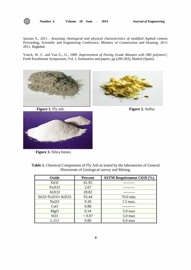
2.2 Fly Ash
Fly ash, a by-product of coal combustion, is widely used as a cementation and pozzolanic
ingredient in Portland cement concrete and asphalt concrete. Fly ash is available in local
markets with low cost. This fly ash has low specific gravity (2.0) as compared with ordinary
Portland cement (3.15), and specific surface area ranged to (500-750) m²/kg. Chemical
components of fly ash are tested in the laboratories of General Directorate of Geological
survey and Mining and given in Table. while Fig.1 present a sample of the fly ash used.
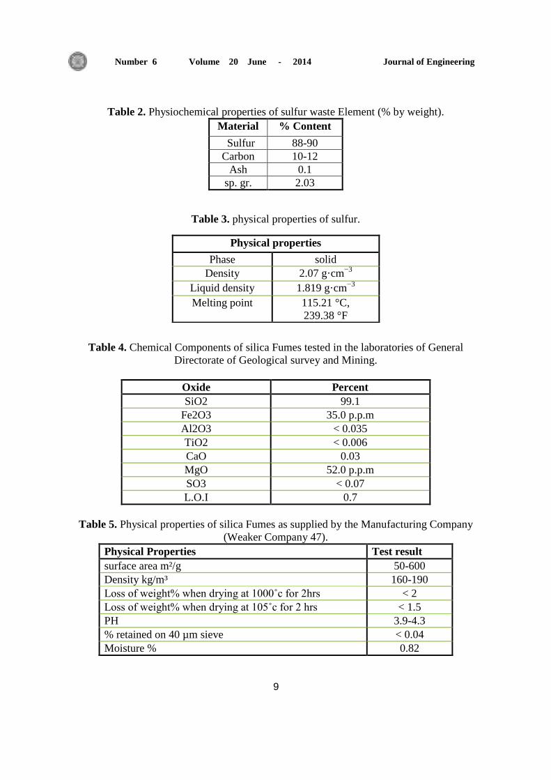
2.3 Sulfur
It was obtained from Al-Meshrak state company (30 km north of Mosul). The
physiochemical properties of these materials are shown in Table 2. Table 3. present physical
properties of sulfur. While Fig2 present sample of the sulfur used.
2.4 Silica Fumes
Silica fumes are produced by a vapor phase hydrolysis process using chlorosilanes such as:
silicon tetrachloride in a flame of hydrogen and oxygen. silica fumes is supplied as a white,
fluffy powder, ACI 234R, 1996. Chemical compositions were tested in the laboratories of

Journal of Engineering Volume 20 June - 2014 Number 6
4
General Directorate of Geological survey and Mining and given in Table 4., The physical
properties are given in Table 5. ,while Fig3. present the silica Fumes sample used.
3. PREPARATION OF MODIFIED ASPHALT CEMENT
3.1 Fly ash-Asphalt cement mix
Asphalt cement has been heated to 160⁰ C for asphalt cement (40-50), 150°C for asphalt
cement (60-70), and the fly ash was added gradually with continuous stirring on the hot
plate for 30 minutes as blending time. Three percentage of the fly ash (5%, 10%, and 15%)
by weight of asphalt cement (40-50) and (60-70) have been implemented. Samples were
subjected to physical properties determination before and after aging process using thin film
oven test.
3.2 Sulfur-Asphalt cement mix
Asphalt cement has been heated to 160⁰ C for asphalt cement (40-50), 150°C for asphalt
cement (60-70), and sulfur was introduced in a powder form to it and mixed using manual
mixing and constant stirring on the hot plate for 30 minutes as blending time.
Three percentage of the sulfur (3%, 5%, and 7%) by weight of asphalt cement (40-50) and
(60-70) have been implemented based on work by Sarsam , 2006. Samples were subjected to
physical properties determination before and after aging process using thin film oven test.
3.3 Silica Fumes -Asphalt cement mix Asphalt cement has been heated to160⁰ C for asphalt
cement (40-50), 150°C for asphalt cement (60-70), and then silica fume was added with
mixing using manual stirring on the hot plate for 45 minutes as a constant blending time.
Three percentage of the silica Fumes (1%, 2%, and 3%) by weight of asphalt cement (40-50)
and (60-70) have been introduced based on previous work by Sarsam (2012). Samples were
subjected to physical properties determination before and after aging process using thin film
oven test.
4. TESTING PROGRAM
4.1 Penetration Test
The penetration test, ASTM D-5 (2002) is an empirical measure of asphalt consistency. In
this test, a container of asphalt cement is placed at the standard test temperature (25°C) in a
temperature-controlled water bath. A prescribed needle, weighted to 100 grams, is placed on
the surface of the asphalt cement for 5 seconds. The depth of penetration, expressed in units
of 0.1mm, is considered the “penetration” of the asphalt cement.
4.2 Softening point test
The softening point test, ASTM D36 (2002) is also used to measure asphalt consistency. The
test is performed by confining asphalt samples in brass rings and loading the samples with
steel balls. The samples are placed in a beaker of water at a specified height above a metal
plate. They are then heated at a specified rate. As the asphalt heats, the weight of the steel
ball pulls the sample down toward the plate. When the sample and ball touch the plate, the
water temperature is measured and designated as the ring and ball softening point of the
asphalt.

Journal of Engineering Volume 20 June - 2014 Number 6
5
4.3 Ductility Test
The ductility of a asphalt cement can be defined as the “distance to which it will elongate
before breaking when two ends of a briquette specimen of the material, are pulled apart at a
specified speed (5cm/min ±5.0%) and at a specified temperature (25±0.50C) ASTM D113-99
(2002). This test method provides measure of tensile properties of bituminous materials and
may be used to measure ductility for specific requirements. Ductility is an indicator of
flexible behavior of asphalt under various temperatures.
4.4Thin film oven test
Physical properties of asphalt cement changes with respect to time and temperature.
Consequently, the performance of pavement will also witness some changes. To take into
account the effects of mixing and compaction temperatures as well as the storage time on the
behavior of asphalt cement and asphalt mixture. All the asphalt samples have been exposed to
accelerated aging by heating the samples in an oven for 5 hours at 163°C .The ASTM D -
1754 (2002) has the satisfied information about this test. Ductility, Penetration and softening
point after thin film oven test have been determined for asphalt cement for all percentage of
modifiers that will be used.
5. DISCUSSIONS ON TEST RESULTS
5.1 Impact of additives on physical properties
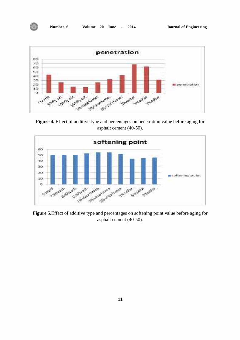
Fly ash was added to the asphalt cement by the percentage of (5, 10 and 15%) by weight of
asphalt cement (40-50) and (60-70). For asphalt cement (40-50), increasing the percentage to
(15%) the penetration was decreased about 68.18%. Figure 4 presents such behavior. The
softening point was (50°C) at (5%fly ash). Increasing the percentage to (15%), the softening
point was increased about 6%. Figure 5 shows the impact. The ductility was (53) at (5% fly
ash).Increasing the percentage to (15%), the ductility was decreased to (28). Figure 6
illustrates such behavior.
For asphalt cement (60-70), increasing the percentage to (15%), the penetration was
decreased about 18.18%. Figure 7 shows such details. At (5% fly ash) the softening point
was (45°C).Increasing the percentage to (15%), the softening point was increased about
6.25%. Figure 8 discusses such behavior. The ductility was (60) at (5% fly ash) .Increasing
the percentage to (15%) the ductility was decreased to (30). Figure 9 demonstrates the
impact on ductility.
Sulfur was added to the asphalt cement by the percentage of (3, 5, and 7%) by weight of
asphalt cement (40-50) and (60-70). For asphalt cement (40-50), increasing the percentage to
(7%), the penetration was decreased by (27.27%). The softening point was decreased to
(44°C) at (3% sulfur).Increasing the percentage to (7%), the softening point was decreased by
8%. The ductility was (+100) at (3% sulfur) .Increasing the percentage to (7%), the ductility
was decreased to (95).
At asphalt cement (60-70) it was noticed that at (3% sulfur) the penetration was increased to
(80).Increasing the percentage over (7%) the penetration was increased by 48.48%. The
softening point was decreased to (45°C) at (3% sulfur) .Increasing the percentage over (7%)
the softening point was decreased about 16.66%. The ductility was (+100) at (3% sulfur).

Journal of Engineering Volume 20 June - 2014 Number 6
6
Silica Fumes was added to the asphalt cement by the percentage of (1, 2 and 3%) by weight
of asphalt cement (40-50) and (60-70). It was noticed that:
At asphalt cement (40-50) increasing the silica fumes percentage to (3%) the penetration was
decreased by 4.5%. The softening point was increased to (55°C) at (1% silica fumes) and
decreased to (52°C) at (3% silica fumes).The ductility was decreased to (19) at (1% silica
fumes) and increased to (25) when using (3%) silica fumes.
At asphalt cement (60-70), increasing the silica fumes percentage to (3%), the penetration
was decreased by 33.3%.
The softening point was increased to (52°C) when a (3%) silica fume was introduced. The
ductility was decreased to (27) at (1% silica fumes) and decreased to (19) when (3%) silica
fumes was adopted.
Table 6 demonstrates the impact of additives on asphalt cement (40-50) properties. While
Table 8 shows the impact of additives on asphalt cement (60-70) properties.
5.2 Impact of additives on aging behavior
The impacts of additives on physical properties of asphalt cement after aging are illustrated in
table 7. The asphalt cement of grade 40-50 has retained 40% of its ductility after aging; the
softening point was increased by 8%, and the penetration was decreased by 36%. When
additives were introduced, their impact was variable; the ductility was reduced by a range of
10-60 % based on additive type and percentage. Sulfur has the least impact on ductility since
it reduces it by 20%. Silica fumes have moderate effect on ductility when it reduces it by
35%, while fly ash shows the highest impact of 36%. The softening point increases after
aging by a range of 6-8% when different percentages and type of additives were introduced.
The penetration value shows variations by a range of 20-60% based on additive type and
percentage.
On the other hand, the asphalt cement of grade 60-70 exhibit 22% reduction in penetration,
6% increment in softening point and 25% reduction in ductility due to aging. When additives
were introduced, sulfur was able to retain its ductility, while fly ash shows moderate
reduction in ductility within a range of 20-36% and silica fumes shows high impact on
ductility in the range of 30-50%.
The impact of additives on softening point was in a range of 3-6% for various percentages
and type of additives. Sulfur shows the lowest impact on penetration in a range of 5-15%,
while fly ash and silica fumes shows higher impact within a range of 17-30%.
Such behavior of additives may be attributed to the increase in viscosity due to high specific
surface area of silica fumes, and to possible chemical reaction took place in case of sulfur and
fly ash.
6. CONCLUSIONS
Based on the testing program, the following conclusions may be drawn:
1. All percentage of additives has reduced the penetration value of asphalt cement, an
exception to that could be noticed when using asphalt cement (40-50) and when adding
sulfur.
2. Softening point was increased with the addition of all percentage of additives except that
with 7% sulfur by wt. of asphalt cement (40-50) it decreased by 8%.

Journal of Engineering Volume 20 June - 2014 Number 6
7
3. Ductility was decreased with the addition of all percentages of additives.
4. For asphalt cement 40-50 after aging, Sulfur has the least impact on ductility since it
reduces it by 20%. Silica fumes have moderate effect on ductility when it reduces it by 35%,
while fly ash shows the highest impact of 36%.
5. The softening point increases after aging by a range of 6-8% when different percentages
and type of additives were introduced. The penetration value shows variations by a range of
20-60% based on additive type and percentage.
6. For asphalt cement 60-70 after aging, sulfur was able to almost retain its ductility, while
fly ash shows moderate reduction in ductility within a range of 20-36% and silica fumes
shows high impact on ductility in the range of 30-50%.
7. The impact of additives on softening point was in a range of 3-6% for various percentages
and type of additives. Sulfur shows the lowest impact on penetration in a range of 5-15%,
while fly ash and silica fumes shows higher impact within a range of 17-30%.
REFERENCES ASTM D-5, 2002 , Standard Test Method for Penetration of Bituminous Materials, American Society
of Testing and Materials.
ASTM D-113, 2002 , Standard Test Method for Ductility of Bituminous Materials, American Society
of Testing and Materials.
ASTM D-1754, 2002 , Standard Test Method for Effects of Heat and Air on Asphaltic Materials
(Thin-Film Oven Test; American Society of Testing and Materials.
ASTM D-36, 2002 “Standard Test Method for Softening Point of Bitumen”, American Society of
Testing and Materials.
Collins, J. H. and Bouldin, M., 1992, "Stability of Straight and Polymer Modified Asphalt", TRB No.
1342, pp (92-100).
Domke, C.H., 1999, Asphalt Compositional Effects on Physical and Chemical Properties,Ph.D.
Dissertation, Texas A&M University.
Sarsam S. Assessing rheological and physical characteristics of modified asphalt cement Proceedings,
8th International Conference on Material Sciences (CSM8-ISM5), Beirut–Lebanon, May 28-30, 2012.
Sarsam S., 2012 , Effect of Silica fumes and Phospho -gypsum on rheological and physical
characteristics of Asphalt cement, Proceedings, Eight International Conference on Material Sciences
(CSM8-ISM5), Beirut–Lebanon, May 28-30, 2012.
Sarsam S., 2008 , Evaluating and testing rheological and physical properties of Mastic Asphalt,
Indian Highways IRC Vol. 36 No.5-2008, India.
Sarsam S., 2006 , Evaluating and testing rheological and physical properties of Mastic Asphalt,
proceeding, IRC Seminar on Innovation in construction and maintenance of flexible pavement-Agra-
India, 2nd -4th September 2006.
Journal of Engineering Volume 20 June - 2014 Number 6
8
Sarsam S., 2011 , Assessing rheological and physical characteristics of modified Asphalt cement,
Proceeding, Scientific and Engineering Conference, Ministry of Construction and Housing, 20-5-
2011, Baghdad.
Vonck, W. C. and Van G., G., 1989 ,Improvement of Paving Grade Bitumen with SBS polymers",
Forth Eurobitume Symposium, Vol. I, Summaries and papers, pp (299-303), Madrid (Spain).
Figure 1. Fly ash. Figure 2. Sulfur.
Figure 3. Silica fumes.
Table 1. Chemical Components of Fly Ash as tested by the laboratories of General
Directorate of Geological survey and Mining.
Oxide Percent ASTM Requirement C618 (%)
SiO2 61.95 ---------
Fe2O3 2.67 ---------
Al2O3 28.82 ---------
SiO2+Fe2O3+Al2O3 93.44 70.0 min.
Na2O 0.26 1.5 max.
CaO 0.88 ----------
MgO 0.34 5.0 max
SO3 < 0.07 5.0 max
L.O.I 0.86 6.0 max
Journal of Engineering Volume 20 June - 2014 Number 6
9
Table 2. Physiochemical properties of sulfur waste Element (% by weight).
Material % Content
Sulfur 88-90
Carbon 10-12
Ash 0.1
sp. gr. 2.03
Table 3. physical properties of sulfur.
Table 4. Chemical Components of silica Fumes tested in the laboratories of General
Directorate of Geological survey and Mining.
Oxide Percent
SiO2 99.1
Fe2O3 35.0 p.p.m
Al2O3 < 0.035
TiO2 < 0.006
CaO 0.03
MgO 52.0 p.p.m
SO3 < 0.07
L.O.I 0.7
Table 5. Physical properties of silica Fumes as supplied by the Manufacturing Company
(Weaker Company 47).
Test result Physical Properties
50-600 surface area m²/g
160-190 Density kg/m³
< 2 Loss of weight% when drying at 1000˚c for 2hrs
< 1.5 Loss of weight% when drying at 105˚c for 2 hrs
3.9-4.3 PH
< 0.04 % retained on 40 µm sieve
0.82 Moisture %
Physical properties
Phase solid
Density 2.07 g·cm−3
Liquid density 1.819 g·cm−3
Melting point 115.21 °C,
239.38 °F

Journal of Engineering Volume 20 June - 2014 Number 6
10
Table 6. Physical properties of Modified Asphalt cement Grade (40-50) before aging.
Asphalt cement
(40-50) Penetration Softening point Ductility
Control 44 50 >100
5%fly ash 25 50 53
10%fly ash 15 50 30
15%fly ash 14 53 28
3% sulfur 68 44 >100
5%sulfur 63 45 97
7%sulfur 50 46 95
1% silica fumes 25 53 19.5
2% silica fumes 32 53.5 21
3% silica fumes 41 51 22
Table 7. Physical properties of Modified Asphalt cement Grade (40-50) after aging.
Asphalt
cement (40-50) Penetration Softening point Ductility
Control 28 54 60
5%fly ash 15 52 33
10%fly ash 11 53 19
15%fly ash 9 55 11
3% sulfur 22 48 81
5%sulfur 50 46 79
7%sulfur 51 46 77
1% silica fumes 33 56 8
2% silica fumes 25 58 19
3% silica fumes 15 57 16
Journal of Engineering Volume 20 June - 2014 Number 6
11
Figure 4. Effect of additive type and percentages on penetration value before aging for
asphalt cement (40-50).
Figure 5.Effect of additive type and percentages on softening point value before aging for
asphalt cement (40-50).

Journal of Engineering Volume 20 June - 2014 Number 6
12
Figure 6. Effect of additive type and percentages on ductility value before aging for asphalt
Cement (40-50).
Table 8. Physical properties of Modified Asphalt cement Grade (60-70) before aging
Asphalt
cement (60-70) Penetration Softening point Ductility
Control 66 48 >100
5%fly ash 52 45 60
10%fly ash 47 46 40
15%fly ash 54 51 30
3% sulfur 80 45 >100
5%sulfur 93 42 >100
7%sulfur 98 40 >100
1% silica fumes 63 48 27
2% silica fumes 57 54 25
3% silica fumes 44 52 19
Journal of Engineering Volume 20 June - 2014 Number 6
13
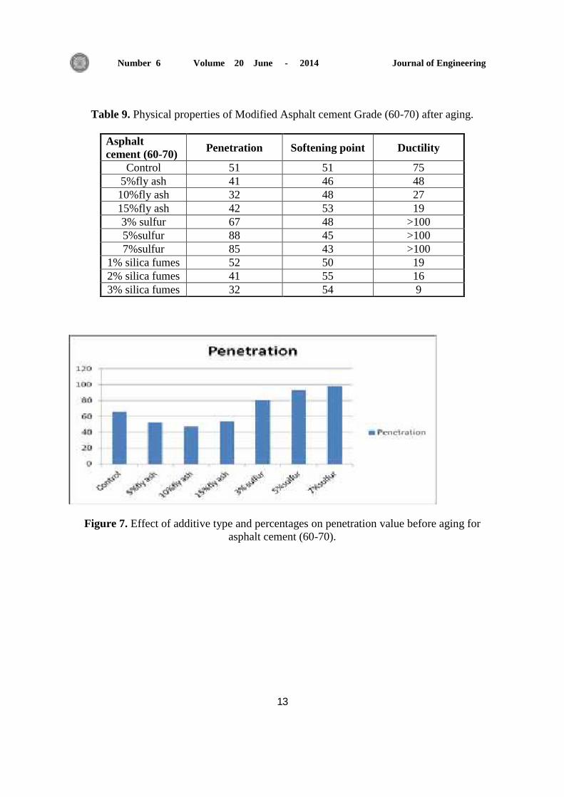
Table 9. Physical properties of Modified Asphalt cement Grade (60-70) after aging.
Figure 7. Effect of additive type and percentages on penetration value before aging for
asphalt cement (60-70).
Asphalt
cement (60-70) Penetration Softening point Ductility
Control 51 51 75
5%fly ash 41 46 48
10%fly ash 32 48 27
15%fly ash 42 53 19
3% sulfur 67 48 >100
5%sulfur 88 45 >100
7%sulfur 85 43 >100
1% silica fumes 52 50 19
2% silica fumes 41 55 16
3% silica fumes 32 54 9

Journal of Engineering Volume 20 June - 2014 Number 6
14
Figure 8. Effect of additive type and percentages on softening point value before aging for
asphalt cement (60-70).
Figure 9. Effect of additive type and percentages on ductility before aging , asphalt cement
(60-70).

Journal of Engineering Volume 20 June - 2014 Number 6
15
Finite Element Analysis of Reinforced Concrete T-Beams with Multiple Web
Openings under Impact Loading
Dr.Nazar Kamel Oukaili Abeer Hussein Al-Shammari
Professor Lecturer
College of Engineering- University of Baghdad College of Engineering-University of Al-Mustansiriya
E-mail: [email protected] E-mail: [email protected]
ABSTRACT
In this study, a three-dimensional finite element analysis using ANSYS 12.1 program had
been employed to simulate simply supported reinforced concrete (RC) T-beams with multiple
web circular openings subjected to an impact loading. Three design parameters were considered,
including size, location and number of the web openings. Twelve models of simply supported
RC T-beams were subjected to one point of transient (impact) loading at mid span. Beams were
simulated and analysis results were obtained in terms of mid span deflection-time histories and
compared with the results of the solid reference one. The maximum mid span deflection is an
important index for evaluating damage levels of the RC beams subjected to impact loading.
Three experimental T-beams were considered in this study for calibration of the program. All
models had an identical cross-section and span similar to those of the experimental beams. The
diameter of the openings of the experimental beams was 110 mm. Three other diameters were
varied (50, 80 and 130) mm. The location of the face of the opening with respect to the location
of impact loading was investigated (the face of the opening at distance varied 0d, 0.5d, 1d and
1.5d from the location of loading, where d is the effective depth) and the number of web
openings was varied (2,4 and 6) openings. All modeled beams subjected to dropping mass of
24.5 kg with height of drop of 250 mm (as for the experimental beams). Results obtained from
this study showed that the behavior of beams with circular openings of diameter equal to 22%
the web depth has a small effect on the response of the RC T-beams. On the other hand,
introducing circular openings with a diameter equal to 35% and 57% of the web depth (80 and
130 mm) increases the maximum mid span deflection by 23% and 43% respectively. Results
also showed that, openings with a distance greater than or equal to 1.5 d from the location of
impact loading have no effect on the deflection of the RC beams.
Key words: beams, web openings, impact loading.
( حاوو على فتحات وتره Tلتحلل بإستخذام العناصر المحذده لعتبات خرسانو مسلحو رات مقطع )ا
متعذده تحت تأثر الحمل الصذم
عبر حسن الشمري زار كامل العقل ن د.
يذسس أصخار
انضايع انضخصشكهت انذص / كهت انذص / صايعت بغذاد
الخالصو
رنك ANSYSف ز انذساص حى عم ححهم رالر األبعاد بئصخخذاو طشقت انعاصش انحذد ع طشق انبشايش انخحهه
ش يخعذد دائش انشكم خاضع نحم صذي. حى إعخاد ( ححخ عه فخحاث حTنخزم عخباث خشصا يضهح راث يقطع )
رس ي انعخباث انخشصا 12رالد يخغشاث حص حضى: حضى يقع عذد انفخحاث. حى حضهظ انحم انصذي عه
يخططاث طل انضهح بضطت اإلصاد ف قط احذ حقع يخصف انفضاء. انخائش انخ حى انحصل عها انخ بذالنت
يخصف انفضاء يع انزي حى يقاسخا يع خائش انرس انشصع انغش حا عه فخحاث حذ إ انطل األقص

Journal of Engineering Volume 20 June - 2014 Number 6
16
يؤشش يى نخحذذ يضخ انضشس نهعخباث انخاضع نهحم انصذي. حى اعخاد خائش رالد عخباث يفحص عها ي أصم
يقطع فضاء يارم نهعخباث انفحص عها. قطش فخحاث انعخباث انفحص عها يعاشة انبشايش. صع انارس نا
يهى( كزنك حى دساصت يقع انفخحاث ضبت ان يقع انحم 130، 80، 50يهى. رالرت أقطاس أخش حى دساصخا )110ضا
فخحاث(. 6، 4، 2عذد انفخحاث يخغش ) ي يقع انحم( كزنك 0d ،0.5d ،1d ،1.5dانصذي )بذات انفخح حخغش بضافت
% ي عق انحش نا حأرش قهم عه طنا. ي اح 22انخائش انضخحصه بج أ انعخباث راث فخحاث دائش بقطش
% 23% ي عق انحش زذ ي انطل األقص نخصف انفضاء بضبت 57 %35أخش فئ عم فخحاث دائش بقطش
ي يقع انحم انصذي نش نا حأرش 1.5dعه انخان. كزنك بج انخائش بأ انفخحاث راث يضاف اكبش أ حضا % 43
.انحا عه حهك انفخحاث عه طل انعخباث
1. INTRODUCTION
Web openings in beams are essential to provide a convenient passage of service ducts and pipes.
As a result, story height of buildings can be reduces and slight reduction in concrete beams
weight would improve the demand on the supporting frame both under gravity loading and
seismic excitation which resulting in major cost saving.
Size of opening did affect strength, but an unreinforced web containing a square opening of one-
quarter the web depth, or a circular opening of three-eighths the web depth, did not reduce the
strength of the specimen ,ASCE-ACI Committee 426. According to Somes and Corley, 1974,
a circular opening may be considered as large when its diameter exceeds 0.25 times the depth of
the web because introduction of such openings reduces the strength of the beam. Mansur, et al.,
1991 made an investigation on eight reinforced concrete continuous beams, each containing a
large transverse opening. Their study showed that an increase in the depth of opening from 140
mm to 220 mm led to a reduction in collapse load from 240 kN to 180 kN.
In practice, there are many incidents in which the structures undergo impact or dynamic loading,
such as during an explosion, transportation structures subjected to vehicle crash impact, impact
of ice load on marine and offshore structures, accidental falling loads, etc. The behavior of
concrete beams subjected to impact loads, is different compared to the behavior under static
loading. Due to the short duration of loading, the strain rate of material is significantly higher
than that under static loading conditions.
At the present time, many methods for analyzing RC members are available. One of the most
powerful methods is the finite element technique which spares much time and efforts. Even
though many experimental studies have been reported, limited research studies have been done
on reinforced concrete T-beam with multiple web openings under impact loading by simulation.
In order to verify the finite element model, three experimental beams (a solid beam without
openings and two other beams with four and six un-strengthened circular openings provided in
the study of Oukaili, and Shammari, 2013 were considered in this study.
2. OBJECTIVES AND SCOPES
The purpose of this study is to investigate the effect of size, location and number of circular web
openings on the impact response of RC T-beams without strengthening of the openings by
additional reinforcement. This research study focuses on three variables:
1. Diameter of openings (50, 80, 110 and 130 mm).
2. Location of openings with respect to the location of impact loading (clear distance between
the impact load and the beginning of opening = 0d, 0.5d, d and 1.5d)
3. Number of web openings (2, 4 and 6 openings).
The scope of this study is to simulate simply supported RC T-beams with the mentioned
variables under transient (impact) loading using ANSYS 12.1 program to obtain mid span
deflection-time histories and compare them with the solid reference beam.

Journal of Engineering Volume 20 June - 2014 Number 6
17
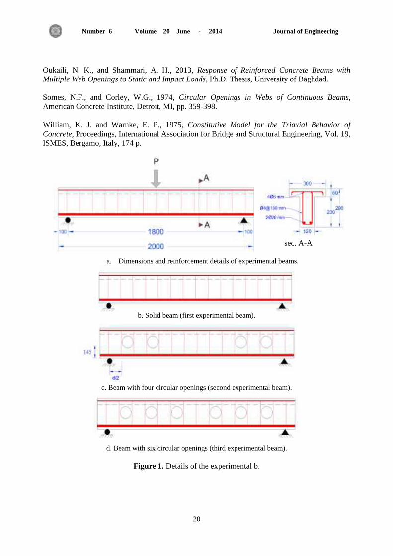
All T-beams have identical dimensions and reinforcement based on Oukaili and Shammari
(2013) experimental beams. Thickness of flange =60mm, width of flange =300mm, depth of
web =230mm and width of web =120mm. Beam length =2000mm with an effective span of
1800mm. All beams were reinforced with 2 20mm longitudinal bars as tension reinforcement,
four 6 mm longitudinal bars as compression reinforcement and 4 mm at 130 mm center to
center as stirrups. The dimensions and details of reinforcement are shown in Fig. 1a.
Fig. 1b-1d shows the details of the experimental beams which were considered in this study for
calibration of the program. The distance between the end of the first opening (near the support)
and the support equals 130 mm; this is about half the effective depth. The centers of the circular
openings were located at 145 mm along the y-direction from soffit of the beam. Diameter of
openings is 110mm (0.48 the web depth).
3. MODELS SPECIFICATIONS
3.1 Material Properties
3.1.1 Concrete
Concrete is a quasi-brittle material and has different behavior in compression and in tension.
Solid65 element was used to model this material. This element has eight nodes with three
degrees of freedom at each node - translation in the nodal x, y, and z directions. This element is
capable of plastic deformation, cracking in three orthogonal directions, and crushing. A
schematic of the element is shown in Fig. 2 ANSYS Manual, Version 12.1. Smeared cracking
approach has been used in modeling the concrete in the present study William, and Wranke,
1975. Poisson?s ratio ( ) for concrete was assumed to be 0.2 ,Bangash, 1989. Self-weight of the
beams was considered.
3.1.2 Reinforcement
Modeling of reinforcing steel in finite elements is much simpler than the modeling of concrete.
A Link 8 element was used to model steel reinforcement. This element is a three dimensional
spar element and it has two nodes with three degrees of freedom -translations in the nodal x, y,
and z directions. This element is also capable of plastic deformation. This element is shown in
Fig. 3. A perfect bond between the concrete and steel reinforcement is considered. However, in
the present study the steel reinforcing was connected between nodes of each adjacent concrete
solid element, so the two materials shared the same nodes. The steel for the finite element
models is assumed to be an elastic-perfectly plastic material and identical in tension and
compression. A Poisson?s ratio of 0.3 is used for the steel reinforcement.
3.2 Boundary Conditions and Loading
Taking advantages of the symmetry, only quarter of the beam was modeled. Rollers were used
to show the symmetry condition at internal faces, whereas the nodes at the support were
restrained against vertical displacement.
Transient dynamic analysis (sometimes called time-history analysis) is a technique used to
determine the dynamic response of a structure under the action of any general time-dependent
loads. This type of analysis can be used to determine the time-varying displacements, strains,
stresses, and forces. Three methods are available in ANSYS program to do a transient dynamic
analysis: full, mode superposition, and reduced. ANSYS analysis was done using the reduced
method; this method condenses the problem size by using master degrees of freedom and
reduced matrices. After the displacements at the master DOF have been calculated, ANSYS
expands the solution to the original full DOF set. Multiple load steps are usually required to
specify the load history in a transient analysis. The first load step is used to establish initial

Journal of Engineering Volume 20 June - 2014 Number 6
18
conditions, and second and subsequent load steps are used for the transient loading. Fig. 4 shows
FE mesh, boundary conditions and load step.
Damping has much less importance in controlling the maximum response of a structure to
impact loads than for periodic or harmonic loads because the maximum response to a particular
impulsive load will be reached in a very short time, before the damping forces can absorb much
energy from the structure, Clough, 2003, for this reason only the undamped response to impact
loads will be considered in this study.
4. VERIFICATION STUDY
The finite element analysis calibration study includes modeling of RC T-beams with dimensions
and properties corresponding to solid beam and two other beams with four and six circular web
openings of diameter equals 110mm tested by Oukaili, and Shammari, 2013. The aim of the
comparison is to ensure that the elements, material properties and convergence criteria are
adequate to model the response of the beams and to be sure that the simulation process is
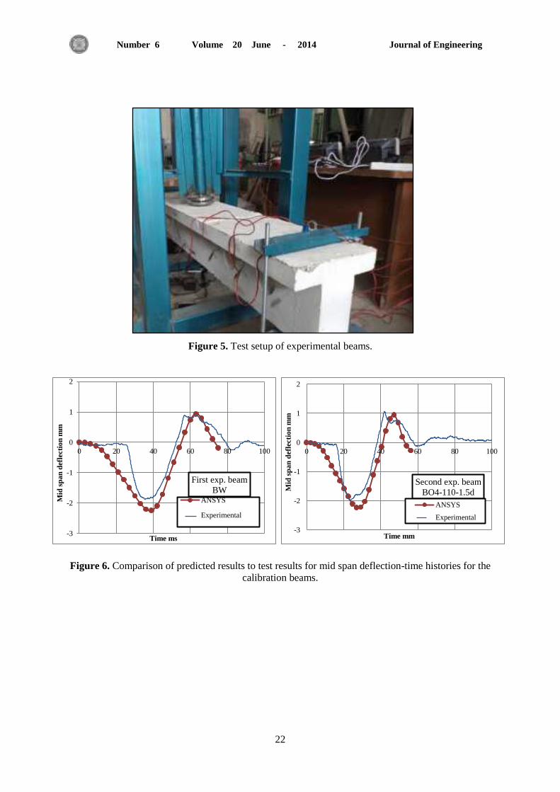
correct, the test setup of the experimental beams is shown in Fig.5.
Transient analyses were made for dropping mass of 24.5 kg and height of drop of 250 mm for
the three experimental beams. Finite element analysis results in terms of mid span deflection-
time histories are shown in Fig. 6. In general, the agreement is good and the plots have similar
trends.
5. PARAMETRIC STUDY
Results and discussion can be presented in three sections according to the parametric study. In
the first section, the finite element modeling of the reinforced concrete beams with circular
openings in varying diameters (50, 80, 110 and 130 mm) will be discussed. In the second
section, the discussion will be made about the effective location of the opening with respect to
the location of the impact loading. In the third section, the effect of different number of openings
(2, 4 and 6) will be presented. These modeled beams have the same dimensions as the
experimental beams tested by Oukaili, and Shammari, 2013. Twelve models were needed for
this study; details of these models were presented in Table 1.
6. RESULTS AND DISCUSSION
6.1 Effect of Size of Web Openings
The transient (impact) response of four RC modeled beams with six openings of distance
between the point of applied load and the beginning of first opening equals 0.5d and with
variable diameter, 50, 80, 110 and 130 mm, was studied. From the analysis results, it was found
that the maximum mid span deflection of the modeled beam with six openings, each of 50 mm
diameter was 2.44 mm while that for the solid one was 2.24 mm. The increase in the maximum
mid span deflection was 8%. Hence, introducing openings with a diameter equal to 22% the web
depth of the beam has a small effect on the deflection of the beam.
On the other hand, it was found that the maximum mid span deflections of the modeled beams
of six openings with 80, 110 and 130 mm diameter six openings were 2.74, 3 and 3.2 mm. The
increase in the maximum mid span deflection was 23%, 34% and 43% compared to the solid
beam. Fig. 7 shows the effect of the size of openings.
6.2 Effect of Location of Web Openings
In this section, the effective location of the opening with respect to the location of the impact
loading that affect the response of the RC beam can be found. Four different locations of two
symmetrical openings were studied, 0d, 0.5d, d and 1.5d from the point of impact loading to the

Journal of Engineering Volume 20 June - 2014 Number 6
19
beginning of the opening. It was found that as the distance of the opening from the point of
impact loading increases, the effect of opening on the response of the RC beams in terms of mid
span deflection-time history decreases till this distance reach 1.5 d ;at this distance, the opening
has no effect on the mid span deflection-time history of the beam. Fig. 8 shows the effect of the
location of openings.
6.3 Effect of Number of Web Openings
In this section, the effect of number of web openings with different locations along the span of
the modeled beams on the impact response of RC beams was presented. From the analysis
results it can be found that the maximum mid span deflections for the modeled beams are of
approximately equal values when the distance of the opening is 0.5d from the applied load
location, regardless the number of web openings (2, 4 or 6 openings). Modeled beam with six
openings which were distributed one close to the other in the middle part of the beam web
showed maximum mid span deflection of 56% greater than that of the solid beam. Fig. 9 shows
the effect of number of openings of different locations on the mid span deflection-time history.
7. CONCLUSIONS
The following conclusions can be obtained from the analysis results. The conclusions are based
on transient analyses which made by dropping mass of 24.5 kg and height of drop of 250 mm as
in the experimental beams:
1. Introducing openings with a diameter equal to 22% the web depth of the beam causes an
increase in the maximum mid span deflection by 8%.
2. The increase in the maximum mid span deflection is 23%, 34% and 43% for beams with six
openings with 80, 110 and 130 mm diameter respectively, compared to the solid beam.
3. As the distance of the opening from the point of impact loading increases, the effect of
opening on the response of the RC beams in terms of mid span deflection-time history decreases
till this distance reaches 1.5 d; at this distance, the opening has no effect on the mid span
deflection-time history of the beam
4. The maximum mid span deflections for the modeled beams are of approximately equal values
when the distance of the opening is 0.5d from the applied load location, regardless the number
of web openings.
5. Modeled beam with six openings which were distributed one close to the other in the middle
part of the beam web showed maximum mid span deflection of 56% greater than that of the
solid beam.
REFERENCES
ACI-ASCE Committee 426, 1974., Shear Strength of Reinforced Concrete Members (ACI
426R-74) (Reapproved 1980), Proceeding, ASCE, V.99, No.ST6, June, pp.1148-1157.
ANSYS, ANSYS User?s Manual Release 12.1, ANSYS, Inc.
Bangash, M.Y. H., 1989, Concrete and Concrete Structures: Numerical Modeling and
Applications, Elsevier Science Publishers Ltd., London, England, 1989.
Clough, R. W., and, Penzien, J., 2003, Dynamics of Structures, Book, Third Edition, USA, 730p.
Mansur, M.A., Lee, Y.F., Tan, K.H. and Lee, S.L., 1991, Test on RC Continuous Beams with
Openings, Journal of Structural Engineering, Vol. 117, No. 6, pp. 1593-1605.
Journal of Engineering Volume 20 June - 2014 Number 6
20
Oukaili, N. K., and Shammari, A. H., 2013, Response of Reinforced Concrete Beams with
Multiple Web Openings to Static and Impact Loads, Ph.D. Thesis, University of Baghdad.
Somes, N.F., and Corley, W.G., 1974, Circular Openings in Webs of Continuous Beams,
American Concrete Institute, Detroit, MI, pp. 359-398.
William, K. J. and Warnke, E. P., 1975, Constitutive Model for the Triaxial Behavior of
Concrete, Proceedings, International Association for Bridge and Structural Engineering, Vol. 19,
ISMES, Bergamo, Italy, 174 p.
sec. A-A
a. Dimensions and reinforcement details of experimental beams.
b. Solid beam (first experimental beam).
c. Beam with four circular openings (second experimental beam).
d. Beam with six circular openings (third experimental beam).
Figure 1. Details of the experimental b.

Journal of Engineering Volume 20 June - 2014 Number 6
21
Figure 2. Solid 65 element geometry.
Figure 3. Link 8 element geometry.
Figure 4. FE mesh, boundary conditions and load step.
Journal of Engineering Volume 20 June - 2014 Number 6
22
-3
-2
-1
0
1
2
0 20 40 60 80 100
Mid
sp
an
defl
ecti
on
mm
Time ms
First exp. beam
BW ANSYS
Experimental
-3
-2
-1
0
1
2
0 20 40 60 80 100
Mid
sp
an
defl
ecti
on
mm
Time mm
Second exp. beam
BO4-110-1.5d
ANSYS
Experimental
Figure 5. Test setup of experimental beams.
Figure 6. Comparison of predicted results to test results for mid span deflection-time histories for the
calibration beams.

Journal of Engineering Volume 20 June - 2014 Number 6
23
Figure 6. Continue, Comparison of predicted results to test results for mid span deflection-time histories
for the calibration beams.
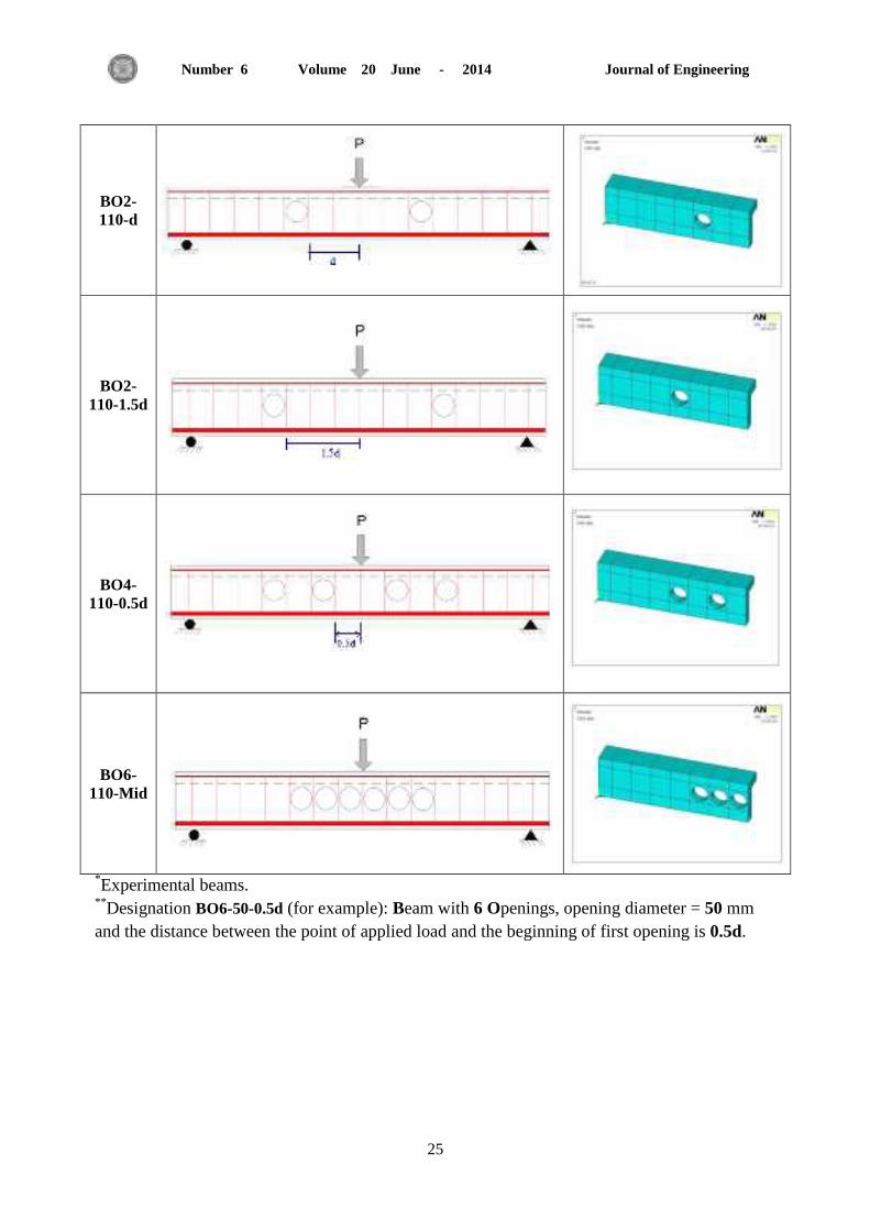
Table 1. Details of the modeled beams.
Quarter modeled beam in
ANSYS Details
Modeled
beam
symbol
*BW
*BO4-
110-1.5d
*BO6-
110-0.5d
-4
-3
-2
-1
0
1
2
0 20 40 60 80 100
Mid
sp
an
defl
ecti
on
mm
Time mm
Third exp. beam
BO6-110-0.5d
ANSYS
Experimental

Journal of Engineering Volume 20 June - 2014 Number 6
24
**BO6-
50-0.5d
BO6-80-
0.5d
BO6-
130-0.5d
BO2-
110-0d
BO2-
110-0.5d
Journal of Engineering Volume 20 June - 2014 Number 6
25
BO2-
110-d
BO2-
110-1.5d
BO4-
110-0.5d
BO6-
110-Mid
*Experimental beams.
**Designation BO6-50-0.5d (for example): Beam with 6 Openings, opening diameter = 50 mm
and the distance between the point of applied load and the beginning of first opening is 0.5d.

Journal of Engineering Volume 20 June - 2014 Number 6
26
Figure 7. Effect of size of circular web openings on mid span deflection-time histories from ANSYS
analyses.
Figure 8. Effect of location of web openings on mid span deflection-time histories from ANSYS
analyses.
-4
-3
-2
-1
0
1
2
0 20 40 60 80 100
Mid
sp
an
def
lect
ion
mm
Time ms
H=250 mm
BW
BO6-50-0.5d
BO6-80-0.5d
BO6-110-0.5d
BO6-130-0.5d
-4
-3
-2
-1
0
1
2
0 20 40 60 80 100
Mid
sp
an
def
lect
ion
mm
Time ms
BW
BO2-110-0d
BO2-110-0.5d
BO2-110-d
BO2-110-1.5d

Journal of Engineering Volume 20 June - 2014 Number 6
27
Figue 9. Effect of number of web openings on mid span deflection-time histories from ANSYS analyses.
-4
-3
-2
-1
0
1
2
0 20 40 60 80 100
Mid
sp
an
def
lect
ion
mm
Time ms
BW
BO2-110-0.5d
BO4-110-0.5d
BO6-110-0.5d
BO6-110-M
Journal of Engineering Volume 20 June - 2014 Number 6
28
Performance Analysis of Four Conceptual Designs for the Air Based
Photovoltaic / Thermal Collectors
Karima Esmail Amori Mustafa Adil Al-Damook
Assistant Professor
Univ. of Baghdad/ Mech. Eng. Dept. , Aljaderiya - Baghdad-Iraq
[email protected] [email protected]
ABSTRACT
The thermal and electrical performance of different designs of air based hybrid
photovoltaic/thermal collectors is investigated experimentally and theoretically. The circulating air
is used to cool PV panels and to collect the absorbed energy to improve their performance. Four
different collectors have been designed, manufactured and instrumented namely; double PV panels
without cooling (model I), single duct double pass collector (model II), double duct single pass
(model III), and single duct single pass (model IV) . Each collector consists of: channel duct, glass
cover, axial fan to circulate air and two PV panel in parallel connection. The temperature of the
upper and lower surfaces of PV panels, air temperature, air flow rate, air pressure drop, wind speed,
solar radiation and ambient temperature were measured. The power produced by solar cells is
measured also. A theoretical model has been developed for the collector model IV based on energy
balance principle. The prediction of the thermal and hydraulic performance was obtained for the
fourth model of PV/T collector by developing a Matlab computer program to solve the numerical
model. The experimental results show that the combined efficiency of model III is higher than that
of models II and IV. The pressure drop of model III is less than that of models I and IV, by (43.67%
and 49%). The average percentage error between the theoretical and experimental results was
9.67%.
Keywords: solar energy; hybrid collector; PV/T; thermal; electrical; performance; air based collector.
فوتوفولطائيةتحليل األداء لتصاميم مختلفة لمجمعات شمسية هوائية حرارية/
سماعيل عموري مصطفى عادل عبد الرحيماكريمة أستاذ مساعد
قسم الميكانيك –كلية الهندسة -جامعة بغداد
الخالصة
. اسخخذو يهدت )فىحىفىنخبئت/ زرارت( هىائت ندؼبث شست األداء انسرار وانكهرببئ نخصبيى يخخهفت حى انخسقق ػهب ي
حى حصى وحصغ وحدهس اربؼت يدؼبث شست االنىاذ. اداءخسس نانطبقت انخصت حدغ انشست ونىاذ انهىاء نخبرذ األ
( ، يدغ رويدري يفرد ويرور I، اندؼبث كبج نىز شس يربىط بذو حبرذ )ىرج بأخهسة انقبش يخخهفت
. خكى كم (IV( ، و يدري يفرد ويرور يفرد)ىرج IIIيرور يفرد نهبئغ)ىرج ( ، يدر يغIIيسدوج نهبئغ )ىرج
يدغ شس ي: يدري، غطبء زخبخ، يروزت يسىرت نخذور انهىاء ونىز شس يربىطب ػه انخىاز. قسج درخت
وهبىط انضغظ نه، سرػت انربذ، األشؼبع درخت زرارة انهىاء، يؼذل خرب انهىاء، انؼهى وانسفه نألنىاذ ، زرارة انسطر
نهدغ انشس انرابغ بأػخبد يبذأ حى ببء ىرج ظر انشس، ودرخت زرارة اندى وانقذرة انخدت ي قبم األنىاذ انشست.
بهغت يبحالة نسم بببء بربيح زبسىب حخ األداء انسرار وانهذرونك نهىرج انرابغ األحسا انسرار. حى انخىصم ان
بج انخبئح انؼهت ا انكفبءة انركبت نهىرج انثبنث كبج اكبر ي حهك انخبصت ببنىرج انثب وانرابغ. ا انىرج انربض.
%(. أ يخىسظ سبت 74% و 76.34هبىط انضغظ نهىرج انثبنث كب اقم ي رنك انسدم نهىرج انثب وانرابغ بقذار )
%.4.34نئىت ب انخبئح انؼهت وانظرت كبج انخطأ ا
طبقت شست، يدغ هد ، زرار، كهرببئ ، اداء ، يدغ هىائ. الكلمات الرئيسية:

Journal of Engineering Volume 20 June - 2014 Number 6
29
1. INTRODUCTION
Photovoltaic thermal hybrid solar collectors (hybrid PV/T systems), are systems that convert
solar radiation into thermal and electrical energy. These systems combine a photovoltaic cell, with a
solar thermal collector which converts part of the solar radiation (electromagnetic radiation
(photons)) into electricity, and the other part is an energy absorbed by the black surface which heats
a flowing fluid. Photovoltaic (PV) cells suffer from a drop in efficiency with the rise in their
temperature.
Many experimental studies have been reported on the photovoltaic-thermal (PV/T) system, Kern
and Russell 1978. presented the concept of PV/T collector using water or air as a fluid for
removing the absorbed energy. Raghuraman 1981. developed two separate one-dimensional
models for the prediction of the thermal and electrical performance of both liquid and air flat plate
(photovoltaic/ thermal) collectors. Garg and Adhikari 1997.analyzed a PV/T air heating system of
a single and double glass covers. Sopian et.al. 2000. developed and tested a double pass
photovoltaic thermal solar collector suitable for solar drying applications. Chow et al. 2003.
investigated the BIPVT options of a hotel building in South China at (22.2o N). The PV/T face was
attached to a full day air conditioned service room to investigate its cooling by means of natural
flow of air behind the PV models. Othman et al. 2005.studied theoretically and experimentally the
PV/T solar air collector with concentrating reflectors. Shahsavar et al. 2010. designed, built and
tested a PV/T air collector in Kerman, Iran under natural and forced convection with two, four and
eight fans operating together to circulate air. Prashant et al. 2011.presented a new design of a
parallel flow solar air heater with packed material in its upper channel to be capable of providing a
higher heat flux compared to the conventional non-porous bed double flow systems. The collector
efficiency of upward-type double-pass flat plate solar air heaters with fins attached and external
recycle is investigated theoretically by Chii et al. 2011, and , Ma et al. 2011. They proposed a
design of a solar collector that is able to provide both hot water and hot air to increase the annual
thermal conversion ratio of solar energy.
The objective of the present work is to identify experimentally the electrical and thermal
performance of PV/T collectors under Iraq climate conditions considering the effect of air flow rate.
2. EXPERIMENTAL WORK
Four different models of hybrid PV/T collectors are designed manufactured and instrumented.
These models are shown in Figs. 1, 2 and 3. In these models two PV modules in parallel connection
are mounted in wooden structure. The air duct was perfectly sealed to avoid air leakage. Air has
been passed through the duct by using a single DC fan of (6 W) power at the duct outlet. The PV/T
system has been mounted on a steel frame with the feasibility to change the inclination angle. The
specifications for PV module and PV/T collector used in this work are given in Tables 1 and 2
respectively. In model II, air flows in a single duct for one pass over and under the absorber as
shown in Fig.1a. In model III air flows in two ducts over and under the PV module in the same
direction with single pass, while in model IV air passes in a single duct below the absorber only, as
shown in Fig. 3.
Twenty two calibrated thermocouples of type k are used to measure the temperatures in this
work. Ten of them are distributed at equal distances at back surface of the panels with three
thermocouples are fixed on the upper surface along the PV panel at distances of (0.1m , 0.3m ,
2.2m) from the inlet. Eight thermocouples are distributed along the air duct of models II, III, and IV
including the inlet and outlet air temperature, and one thermocouple is fixed on the collector glass
cover, as shown in Fig.4. The ambient temperature was measured at 1.5m above ground. All
thermocouples are connected to a selector switch type K. The air velocity was measured using a
multifunctional anemometer device (model (EM-9000). The air pressure drop is measured using

Journal of Engineering Volume 20 June - 2014 Number 6
30
inclined differential manometer between two points namely ducts’ inlet and outlet as shown in
Fig.1a. The pressure drop is calculated from manometers reading (H) as
sin.Hp (1)
where θ is manometer inclination angle.
The solar radiation is measured by using south facing Solar meter (TES-1333R Data logging)
at the same collector tilt angle.
The power generated by the PV panels was calculated according to the equation:
I*VPpv (2)
where V is the voltage and I is the current produced by PV panels. These parameters are measured
by multimeter model (3500/3600) made in England especially for AC or DC applications.
2.1 Experimental Procedure
The test of the PV/T collectors and PV array for eight months from December 2010 to July
2011 includes.
1. Testing model I without load for ten clear days and with different flow rate ranging from [36.2-
83.1] l/s. This test was carried out during December, 2010 and January, 2011.
2. The data of model I & model II were taken at the same time for ten clear days with different flow
rate ranging from [66.62-126.5] l/s during February & March, 2011.
3. Model III is tested at flow rate [66.62-126.5] l/s with the same manner in 1 and 2 above during
April & May 2011.
4. Model IV is tested during July 2011.
3. THEORETICAL MODEL
The fourth model used in this work is composed of a single glass cover, a PV modules and a
well insolated back plate as shown in Fig.5. The energy balance principle is applied on each
element with the following assumptions: The system is in a quasi-steady state condition, There is no
air leakage from the hydraulically smooth flow channel, Heat capacity of the glass cover, enclosed
air, PV modules absorber and bottom plates are negligible at steady state, The temperatures of the
PV modules, glass, absorber and bottom plates vary only along the x-direction of the air flow, and
heat loss from the sides of the duct is very small and hence neglected , Duffie, and Beckman 1990.
Fig.5 shows the various heat transfer coefficient along the surface of the system.
Absorber PV/T (Fig. 6)
( ) ( ) ( ) (3)
Bottom Plate (Fig. 7) (Al-Damook 2011)
( ) ( ) ( ) (4)
3.1 Calculation of Heat Transfer Coefficients
3.1.1 Heat Loss Coefficients
The overall heat loss factor consists of top, bottom, and edge heat loss coefficients.
The bottom loss coefficient (Ub) is evaluated by considering conduction and convection losses from
the absorber PV/T in the downward direction through the bottom of the collector. It can be
evaluated as: (Sumeet 2010)
1
1
ww
w
c
c
bhK
L
K
LU (5)

Journal of Engineering Volume 20 June - 2014 Number 6
31
where wh is the wind heat transfer coefficient, which is calculated from: McAdams model ,
Francis 2002.
h . . ind (6)
The top heat loss is given by: , Duffie, and Beckman 1990.
1
11
rpcpcrww
thhhh
U (7)
where,
rwh radiation heat transfer coefficient between cover glass and the sky given as:
hr g ( c s
)( c s) (8)
g glass emittance
Stefan-Boltzmanns’ constant equals to 5.67*10-8
W/m2.K
4
sT sky temperature is usually calculated from:
(9)
rpch radiant heat transfer coefficient from absorber PV/T to cover is given as:
111
22
gp
cpmcpm
rpc
)TT)(TT(h
(10)
where ,p g plate and glass emittance.
3.1.2 Heat Transfer Coefficient in the Upper Channel
The natural convection heat transfer coefficient (pch ) between the absorber plate and glass
cover of the collector model IV is estimated by the equation proposed by Meyer et al. (Hussam
2011) as:
u c r n (11)
where, c and n are constants affected by the tilt angle. These constants are listed in table (3).
The Grashof No. (Gr) is defined as
2
3
mapv L)TT(gGr
(12)
where: g=Gravitational acceleration (m/s2). βv=volumetric expansion coefficient (K-1) given as:
Tv
1 (13)
mL Mean space between absorber plate and glass cover (m).
Kinematic air viscosity (m2/s).
The convective heat transfer coefficient is then calculated as:

Journal of Engineering Volume 20 June - 2014 Number 6
32
m
a
pcL
NuKh (14)
where aK is air thermal conductivity (W/m.K)
3.1.3 Heat Transfer Coefficient in Lower Channel
The forced convection heat transfer coefficient between air stream and absorber plate (hf) of
collector model IV and the properties of air are calculated at local fluid temperature (Tf) by: ,Duffie,
and Beckman1990.
uf e r (15)
where:
e
( ) (16)
hD The hydraulic diameter of the air passage is calculated as:
hL
hLDh
2
22 (17)
where 2L collector width, h is duct inlet height,
m air flow rate (kg/s.).
μ air dynamic viscosity (kg/m.s)
Thus, the convective heat transfer coefficient can be obtained as:
hf a
h uf (18)
A Matlab computer program is developed to solve the numerical model. Fig 8. illustrates the flow
chart of this program.
4. RESULTS AND DISCUSSION
Fig.)9 shows the ambient conditions in Fallujah city for selected clear days during the test
period namely; (28/12/2010, 28/7/2011 and 2/7/2011. The ambient temperature follows the incident
solar radiation from sunrise to solar noon, after which a considerable deviation in its behavior is
indicated in April and July.
Fig.10 demonstrates the effect of PV panel temperature on electrical power generated at
different flow rates for models (I , II and III) . It is obvious that the electrical power increases when
the panel temperature decreases.
Fig.11 presents the hourly distribution of combined efficiency, thermal efficiency and
electrical efficiency for models I, II and III. Table (4) illustrates a comparison between the electrical
and combined efficiencies of models II, and III with model I higher efficiency was recorded for
model III.
Fig.12 shows the effect of air flow rate on average PV panel temperature. The heat transfer
coefficient increases with increasing of mass flow rate which leads to absorb more heat and
decrease the temperature difference between the surface panel and flowing air. This result agrees
with that obtained by (Jin et al. 2010).
Fig. 13 demonstrates the effect of Reynolds number on pressure drop for models II & III. It is
clear that the pressure drop increases with increasing of Reynolds number according to:

Journal of Engineering Volume 20 June - 2014 Number 6
33
2
5
2
Re)D
L(flosspressure
h
f
(19)
Fig. 14a shows a comparison between the electrical power produced by models I and II on
29/3/2011. Lower values are indicated for model I than that for model II due to: optical losses, edge
losses, difficulty of cleaning the panel, which leads to dust accumulation on the panels.
Fig.14b demonstrates hourly temperature distribution of the upper and lower PV panel
surfaces on (29/3/2011) for models I & II. The maximum temperature differences between model I
and II for the upper and lower surfaces were 14.94 oC and 15.2
oC, respectively and the minimum
temperature differences were 2.11oC and 6.7
oC, respectively.
4.1 Comparison with Previous Published Results
A quantitative comparison between the present results and previously reported results is
difficult due to the differences in local ambient conditions such as; solar radiation, ambient
temperature, wind speed, humidity and the type of the solar panel used. So a qualitative comparison
have been adopted as shown in Fig.15, which illustrates a very good agreement between the
present work and the previously published results.
4.2 Comparison between Theoretical and Experimental Values for Model IV Fig.16 presents good agreement between theoretical and experimental results of air
temperature in the lower channel for model IV. The maximum percentage deviation is 3.41%.
Fig.17 demonstrates a comparison between theoretical and experimental values of heat gain
for model IV. The deviation between them is due to the optical losses because of dust accumulation.
The percentage error was 13.2%.
Fig.18 illustrates a comparison between theoretical and experimental values for thermal
efficiency. The deviation between them is due to several factor namely:
Fluctuated wind speed values.
Over all heat transfer coefficient.
Variation in real ambient temperature.
Optical losses.
The maximum percentage deviation was 7.6%.
4.3 Comparison between the Four Models for Multi Parameters
The maximum average parameter values for all measured days (thermal efficiency, electrical
efficiency, pressure drop, power consumed (pc) due to air mass flow rate, power of fan, temperature
rise and Reynolds number are given in Table (5) . This table also demonstrates the percentage
enhancement for any parameter which is calculated as:
(20)
5. CONCLUSIONS
From the experimental investigation of the models I, II, III and IV in Iraq climate conditions,
the following conclusions can be concluded. The electric efficiency was a function of PV panel
temperature; the increase of temperature above the design temperature decreases the efficiency of
the panel. It is found that the acceptable range of temperature and solar radiation were (22oC-38
oC)
and (550 ‒ 850) W/m2 respectively, and depending on the grade of PV panel used (A, B, C). The
thermal efficiency of model III was 102.7 % greater than that of model IV. The thermal efficiency
of model III is 26.9 % greater than that of model I. The combined efficiency of model III was 90.4
% greater than that of model IV. The combined efficiency of model III is 5.91 times the efficiency
of model I. The total efficiency (combined efficiency) of model III was 9.45 times that of model II
in the measured days. The combined efficiency of model (I) is 7.29 times greater than that of model

Journal of Engineering Volume 20 June - 2014 Number 6
34
II in the measured days. The pressure drop inside the duct of model III was 43.67 % less than that
of model I in the measured during days despite the fact that mass flow rate for model III was greater
than that of model I. The thermal behavior was improved by increasing the flow rate above 130 L/s
when the range of solar radiation was above 530 W/m2. The average percentage error between
theoretical and experimental results was 9.67%.
REFERENCES
- Alghareeb, A. A.,1992, The effect of thermal radiation and heat transfer area on the performance
of a solar air heater, M.Sc. thesis, univ. of Basrah, Chemical Engineering.
- ASHRAE Applications Handbook, 1999. Chapter 32 by American Society of Heating, Solar
Energy Use (ASHRAE). Atlanta, GA.
- Baa, Y. and Adam, N. 2008, Performance analysis for flat plate collector with and without porous
media, Journal of Energy in Southern Africa, V.19, No 4.
- Chii, D. H., HoMing, Y., Tsung, C. C., 2011, Collector efficiency of upward-type double pass
solar air heaters with fins attached, International Communications in Heat and Mass Transfer,
V.38, pp. 49‒56.
- Chow, T. T., Hand, J. W., Strachan, P. A., 2003, Building-integrated photovoltaic and thermal
applications in a subtropical hotel building, Applied Thermal Engineering, V.23(16),pp.2035-2049.
- Duffie, J.A., Beckman, W. A., 1990, Solar Engineering of Thermal Processes , John Wiley &
Sons, Inc.
- Francis, W., 2002, Heat transfer loss or gain) coefficients from bare flat plate solar heat
collectors, The Zomeworks Program Office of the Double Play System: Summer Cooling and
Winter Heating.
- Garg, H. P., Adhikari, R. S., 1997, Conventional hybrid Photovoltaic∕Thermal (PV/T) air heating
collectors: steady-state simulation, Renewable Energy, V.11, No.3, PP.363-385.
- Hussam, H. J., 2011, Evaluation of a solar assisted desiccant cooling system for a small meeting
hall, M.Sc thesis, university of Baghdad in Mechanical Engineering.
- Jin, L.G., Ibrahim, A., Chean, Y.K., Daghigh, R., Ruslan, H., Mat, S., Othman, M.Y., Sopian, K.,
2010, Evaluation of Single-Pass Photovoltaic-Thermal Air Collector with Rectangle Tunnel
Absorber, American Journal of Applied Sciences, V.7 (2), pp.277-282.
- Kern Jr. EC, Russell Mc., 1978, Combined Photovoltaic and Thermal Hybrid Collector System,
Proceedings of 13th
IEEE Photovoltaic Specialist pp.1153‒7.
- Ma J., Sun, W., Ji J., Zhang, Y., Zhang, A., Fan, W., 2011, Experimental and theoretical study of
the efficiency of a dual-function solar collector, App. Thermal Eng., V.31, pp.1751‒ 1756.
- Mustafa Adil AlDamook, 2011, Performance analysis of various conceptual design for the air
based Photovoltaic/Thermal collectors, M.Sc. thesis, Univ. of Baghdad, Dept. of Mech. Eng.

Journal of Engineering Volume 20 June - 2014 Number 6
35
- Otham, M. H., Yatim, B., Sopian, K., AbuBakar, M. N., 2005, Performance analysis of a double-
pass photovoltaic/thermal (PV/T) solar Collector with CPC and Fins, Renewable Energy V.30,pp
.2005-2017.
- Othman YM, Yatim B, Sopian K, AbuBakar M.N., 2007, Performance studies on a finned
double-pass photovoltaic-thermal (PV/T) solar collector, Desalination V209, pp.43-49.
- Prashant, D., Thakur, N. S., Kumar, A., Singh,S., 2011, An analytical model to predict the thermal
performance of a novel parallel flow packed bed solar air heater, Applied Energy,V.88 , pp. 2157-
2167.
- Raghuraman, P., 1981, Analytical predictions of liquid and air photovoltaic/Thermal flat plate
collect performance, J. of solar energy eng., V. 103, Nov., PP. 291-298.
- Shahsavar, A., Ameri, M., 2010, Experimental investigation and modeling of a direct coupled
PV/T air collector, Solar Energy, V.84, pp.1938-1958.
- Sopian, K., Liu, H. T., Kakac, S., Veziroglu, T. N., 2000, Performance of a double pass
photovoltaic thermal solar collector suitable for solar drying systems, Energy Conversion and
Management, V.41, pp.353-365.
- Sopian K., Alghoul M. A., Alfegi E. M., Sulaiman M. Y. and Musa E A., 2009, Evaluation of
thermal efficiency of double-pass solar collector with porous–non porous media, Renewable
Energy, V.34, pp.640‒645.
- Sumeet, S., 2010, Mathematical modeling of solar air heater with different geometries, M.Sc.
thesis, Thapar University, Patiala Mechanical Eng. Dept.
NOMENCLATURE
Latin Symbols Re Reynolds No.
Ac area of PV cell m2
S Solar radiation (W/m2)
Ap area of absorber plate m2 Sg energy absorbed by the glass cover
(W/m2)
Cp air specific heat (J/kg.K) Sp energy absorbed by the absorber plate
(W/m2)
CFD Computational fluid dynamics tc thickness of PV cells (m)
D depth of air duct (m) tg thickness of glass cover (m)
Dh hydraulic diameter of the air duct (m) tin thickness of insulation (m)
dx length of Elemental duct division (m) aT Ambient air temperature (K).
e root mean square of percentage
deviation bmT bottom plate temperature (K)
F Packing factor fT fluid (air) temperature (K)
g gravitational acceleration (m/s2) gT Collector glass cover temperature (K).
G incident solar radiation (W/m2)
pmT absorber (PV module) temperature (K).
H manometer reading (m) refT reference temperature (K).
hf fluid convection heat transfer
coefficient (W/m2K)
sT sky temperature (K).

Journal of Engineering Volume 20 June - 2014 Number 6
36
hp forced convection heat transfer
coefficient (W/m2K)
Vpv PV voltage (volt)
gph free heat transfer coefficient in the air
gap (W/m2)
Vw wind velocity (m/s)
skyg,rh
radiation heat transfer coefficient
between absorber PV/T and sky
(W/m2K)
W width of the air duct (m)
pb,rh radiation heat transfer coefficient
between absorber PV/T and bottom
plate (W/m2K)
Ut Overall top heat loss coefficient
(W/m2.K)
pg,rh radiation heat transfer coefficient
between absorber PV/T and glass cover
(W/m2K)
V PV voltage (Volt)
wh wind heat transfer coefficient (W/m2.K), x distance along the duct
I PV current (Amp.) Greek Symbols
Kc thermal conductivity of bottom plate
(W/m.K) c absorptivity of cells
Kin thermal conductivity of insulation (m)
Kw thermal conductivity of wood (m) p absorptivity of the plate
L length of absorber plate (m) collector tilt angle (deg)
L1 Collector Length (m) g glass emittance
L2 Collector width (m) p Plate emittance
Lc thickness of bottom plate (m) ηc conversion efficiency of PV module
Lw thickness of wood (m) μ dynamic viscosity (kg/m.s)
m air mass flow rate, (kg/s) density of manometer fluid (kg/m
3)
p pressure drop (Pa) Stephen-Boltzmann constant
Ppv power produced by PV (W) manometer tilt angle (deg)
r linear coefficient of correlation
g transmissivity of glass
Ra air gap Rayleigh No. po transmissivity of pottant

Journal of Engineering Volume 20 June - 2014 Number 6
37
Table 1. Specification of PV/T collectors.
44o(II), 23
o (III), 5
o (VI)
(ASHRAE Handbook 1999) Collector tilt angle (degree)
3310 Collector length (mm)
580 Collector width (mm)
60 Overall height (mm)
35 Upper duct height (mm)
24 Lower duct height (mm)
70×540 model II
10.2×540 model III Inlet area(mm
2)
70×540 model II, model III outlet area(mm2)
Flat plate Plate type
Ordinary clear glass, τ . 6
[Sopain et al. (2009)] Cover material
1 Number of covers
k= 0.059 (Hussam 2011) Thermal conductivity of Insulation
material (Wood panel)
20 Back insulation thickness (mm)
Table 2. Specification of PV panel.
ELECTRICAL DATA
Maximum Power at STC 60 W
Maximum Power voltage at STC 17.6 V
Maximum Power Current at STC 3.4 Amp
Open Circuit Voltage (Voc) 21.6
Short Circuit Current (Isc) 3.74
Operating Temperature 25(oC)
Operating Radiation 1000W/m2
MECHANICAL DATA
Cell Type Poly-crystalline
No. of cells and cells Arrangement 60 (6 x 10)
Dimensions(mm) 1200 x 540 x 32mm
Weight 20kg (44.1 lbs)
Front Cover Tempered glass
Frame Material Anodized Aluminum Alloy
Standard Packaging (Modules per Pallet) 20 pcs
لغيت
الخلفية
الحمرة

Journal of Engineering Volume 20 June - 2014 Number 6
38
Table 3. Constants for Eq.(10).
Tilt angle c n
0 0.060 0.410
10 0.065 0.400
20 0.070 0.390
30 0.075 0.380
40 0.080 0.367
Table (4): Comparison between PV/T collectors.
(Values are taken at solar noon)
Compare between Models Combined
Efficiency%
Electrical
Efficiency Ratio B/A
I and II
A=9.55 (model I) 9.55 (model I)
7.2
B=44 (model II) 9.3 (model II)
III and II A= 44 (model II) 9.3 (model II)
1.32 B= 58 (model III) 6 (model III)
Table (5): Comparison between daily performance parameters for models II, III, IV.
Parameter
Model II
Model III
Model IV
Enhancement ratio%
for (model)
Combined efficiency 65.4 78.7 41.35 90.4%(III)
Thermal efficiency 57.1 72.5 35.8 102.7%(III)
( ) 73.5 41.4 77.44 49%(III)
Pc(mW) 67 57.8 95.75 39.7%(III)
Temp. rise(oC) 7.2 6.23 8.1 30%(IV)
Power fan( ) 33 47 47 21.2(I)

Journal of Engineering Volume 20 June - 2014 Number 6
39
Figure 1. (a) Schematic diagram of experimental setup for model II; (b) Top view of PV
panels; (b) Cross section view of C-C, (d) Outdoor test of model I and model II

Journal of Engineering Volume 20 June - 2014 Number 6
40
Figure 2. Schematic Diagram of Experimental Setup for Model III.
Figure 3. Schematic Diagram of Experimental Setup for Model IV
Figure 4. (a) Cross section of the layers for model I,
(b) Top view of PV panel, (c) Thermocouples positions.

Journal of Engineering Volume 20 June - 2014 Number 6
41
(a) (b)
Figure 5. (a) Various Heat transfer coefficient along the surface of the system. (b)schematic
diagram of the studied PV/T air system (Model IV).
Figure 6. Energy equations for absorber PV/T for
model iv
Figure 7. Energy equations for absorber
bottom plate for model IV

Journal of Engineering Volume 20 June - 2014 Number 6
42
Figure 8. Flow chart of the computer program

Journal of Engineering Volume 20 June - 2014 Number 6
43
Figure 9. Hourly variation of solar
radiation and ambient temperature
for selected days from December
2010 to July 2011
Figure 10. Effect of PV panel
temp. on electric power for three
models (a) model II (b) model III
(c) model IV
Figure 11. Hourly total efficiency,
thermal efficiency and electrical
efficiency for a) model II, b)
model III, c) models I and III
Figure 12. Effect of daily air flow
rate on PV panel temp. for models
II & III
Figure 13. Effect of Reynolds
number on pressure drop for
models II & III
Figure 14. (a) Hourly electrical
power produced by models I& II
on (29/3/2011) (b) Hourly
temperature distribution of the
upper and lower PV panel on
(29/3/2011) for models I&II
(a)
(b)
(c)
(a)
(b)
(c)
Model I
Model III
Model I
Model III
(a)
(b)
Model II Model II

Journal of Engineering Volume 20 June - 2014 Number 6
44
Effect of air mass flow rate on temperature of PV module for collector model II,
(a) present results, (a1) results of (Jin et al. 2010)
Effect of air mass flow rate on pressure drop for collector model II,
(b) present results, (b1) results of (Baa 2008)
Effect of mass flow rate on electrical efficiency PV module for collector model III,
(c) present results, (c1) results of (Jin et al. 2010)
0.03 0.04 0.05 0.06 0.07 0.08 0.09 0.10
flow rate (kg/s)
0
10
20
30
40
50
60
70
80P
V T
emp
. (
C)
present work model II
(a)
o
0.00 0.01 0.02 0.03 0.04 0.05 0.06 0.07 0.08
mass flow rate (kg/s)
0
10
20
30
40
50
60
70
80
PV
Tem
p. (
C)
(a1)
o
without tunnel
with tunnel
0.03 0.04 0.05 0.06 0.07 0.08 0.09 0.10
flow rate (kg/s)
20
30
40
50
60
70
80
90
pes
sure
dro
p (
Pa)
present work model II
(b)
0.02 0.03 0.04 0.05 0.06 0.07
flow rate (kg/s)
0.0
0.5
1.0
1.5
2.0
2.5
3.0
pes
sure
dro
p (
Pa)
(b1)
L=2.4 m
L=1.5 m
0.09 0.10 0.11 0.12 0.13 0.14
flow rate (kg/s)
5.0
5.2
5.4
5.6
5.8
6.0
6.2
6.4
6.6
6.8
7.0
elec
tric
al
effi
cien
cy %
present work model III
(c)
0.00 0.01 0.02 0.03 0.04 0.05 0.06 0.07 0.08
flow rate (kg/s)
0
2
4
6
8
10
12
elec
tric
al
effi
cien
cy %
(c1)
without tunnel
with tunnel

Journal of Engineering Volume 20 June - 2014 Number 6
45
Effect of mass flow rate on air temperature rise for collector model III,
(d) present results, (d1) results of (Othman et al.2007) Figure 15. Comparison of the present results with previously published results.
Figure 16. Comparison between theoretical
and experimental values of hourly air
temperature on (2/7/2011) for model IV
Figure 17. hourly comparison between theoretical
and experimental values of hourly heat gain on
(2/7/2011) for model IV
Figure 18. Comparison between theoretical and experimental values of hourly
thermal efficiency on (2/7/2011) for model IV
0.09 0.10 0.11 0.12 0.13 0.14
flow rate (kg/s)
4.8
5.0
5.2
5.4
5.6
5.8
6.0
6.2
6.4air
tem
p. ri
se (
C)
present work model III
(d)
o
0.00 0.05 0.10 0.15 0.20
flow rate (kg/s)
0
1
2
3
4
5
6
7
8
9
air
tem
p. ri
se (
T -
T )
( C
) (d1)
o
io
theoretical
experimental

Journal of Engineering Volume 20 June - 2014 Number 6
68
Modeling of Electron and Lattice Temperature Distribution
Through Lifetime of Plasma Plume
Chief of Engineers: Ali Hamza Alwan Al-taee
Gas Filling Company
Ministry of Oil
Email: [email protected]
ABSTRACT
When employing shorter (sub picosecond) laser pulses, in ablation kinetics the features
appear which can no longer be described in the context of the conventional thermal model.
Meanwhile, the ablation of materials with the aid of ultra-short (sub picosecond) laser pulses is
applied for micromechanical processing.
Physical mechanisms and theoretical models of laser ablation are discussed. Typical
associated phenomena are qualitatively regarded and methods for studying them quantitatively
are considered. Calculated results relevant to ablation kinetics for a number of substances are
presented and compared with experimental data. Ultra short laser ablation with two-temperature
model was quantitatively investigated. A two-temperature model for the description of transition
phenomena in a non-equilibrium electron gas and a lattice under picosecond laser irradiation is
proposed. Some characteristics are hard to measure directly at all. That is why the analysis of
physical mechanisms involved in the ablation process by ultra-short laser pulses has to be
performed on the basis of a theoretical consideration of `indirect' experimental data.
For Copper and Nickel metal targets, the two-temperature model calculations explain that
the temperature of the electron subsystem increased suddenly and approached a peak value at the
end of laser pulse. In addition, the temperature profile of lattice temperature subsystem evolution
slowly, and still increasing after the end of laser pulse. A good agreement prevails when a
comparison between the present results and published results.
Key words: pulsed laser, heat ablation by laser, two-temperature model, plasma plume.
االلكتزوناث و الشبكت خالل فتزة تكون غيمت البالسمانمذجت توسيع درجت حزارة
علي حمشة علوان الطائي >سئظ يهذع
ششكخ رؼجئخ انغبص
وصاسح انفؾ
خالصتال
10 )الم ي جؼبد انهضس أنمظشح اعزخذاو ػذ-12
Sec. ،)وطفهب فخظبئض ال ك رظهش انززسخ حشكخ ف
جؼبد ثذػى انىاد نزا فب رشغم انؼبد انكبك )ثمبظ يبكشوخ( زى ادبص ثززسخ. انزمهذخ انحشاسخ برجان عبق
. ثكى ثبخ( )الم ي انمظش فبئمخ انهضس
ف انجحث انحبن رى يبلشخ انبد انفضبئخ وانبرج انظشخ نهززسخ ثىاعطخ انظبدس انهضسخ انجؼخ. انظىاهش
ثطشق كخ. نؼذد ي انىاد, انزبئح راد انظهخ ثحشكخ انززسخ رى ػشػهب رى ثحثهب فمخ رؼزجش ىػخ و انىرخخ انشا
. انززسخ ثىاعطخ انظبدس انهضسخ انجؼخ فبئمخ انمظش عبثمب واظهشد رىافك خذ ويمبسزهب يغ انجببد انزدشجخ انشىسح
ك. نجب انظىاهش غش انزىاصخ و االزمبنخ نخهؾ " غبص هم سح وكب انزحرذ دساعزهب ثبعزخذاو ىرج ثبئ دسخخ انحشا
االى" ثغجت اإلشؼبع انغبلؾ ي يظبدس نضسخ يجؼخ فبئمخ انمظش لذ رى الزشاذ اعزخذاو انىرج ثبئ دسخخ -االنكزشوبد
انززسخ ثىاعطخ انظبدس انهضسخ انجؼخ لذ دساعخ آنخ ػمانحشاسح. ثؼغ انخىاص ظؼت لبعهب ثشكم يجبشش. نزا فب
رى ادبصهب ثشاػبح االػزجبساد انظشخ غش انجبششح انز رى انحظىل ػههب ي ردبسة ػهخ عبثمخ.
Journal of Engineering Volume 20 June - 2014 Number 6
69
انحغبثبد انظشخ ثبعزخذاو ىرج ثبئ دسخخ انحشاسح ثذ ا دسخخ حشاسح االنكزشوبد رضداد ثشكم عشغ و
دسخخ حشاسح انشجكخ ف رضداد خ ػذ هبخ جؼخ انهضس ػذ اعزخذاو انحبط او انكم كؼذ هذف. يفشؽ ورظم اللظى ل
ورغزش ثبنزبي ثؼذ ازهبء انجؼخ. لخ دسخخ حشاسح انشجكخ دائب الم ي دسخخ حشاسح االنكزشوبد. ,هبخ صي جؼخ انهضس
اخفبع يؼذل انززسخ خالل صي جؼخ انهضس. ػؼف انزشاثؾ ث االنكزشوبد و انشجكخ ؤدي انى
بنهضس, ىرج ثبئ دسخخ انحشاسح, غخ انجالصيب.ثنضس يجغ, رزسخ يسيت:ئالكلماث الز
1. INTRODUCTION
Ablation occurred when solid surface exposure to an intense laser irradiation.
As a result atoms or clusters may emit from the target surface. For the ultra-short laser
pulse duration, there is a variation in the temperature between electrons and lattice
sub-systems. Two temperature model one of the approaches can be applied to
investigate the temperature profiles throughout the laser target.
Schäfer, et al., 2002, investigated picosecond laser ablation of metals by
using a hybrid simulation scheme. Laser energy input into the electron system and
heat conduction within it are modeled using a finite-difference scheme for solving the
heat conduction equation. Energy transfer between the electronic and atomic
subsystems due to electron-phonon coupling is taken into account. Zhigilei, et al.,
2002,discussed two computational schemes developed for simulation of laser
coupling to organic materials and metals and present a multi-scale model for laser
ablation and cluster deposition of nano-structured materials. For metals, the two
temperature model coupled to the atomistic (molecular dynamics) MD model
provides an adequate description of the laser energy absorption into the electronic
system and fast electron heat conduction. Korte, et al., 2000, investigated the
production sub-diffraction limited structures in thin metal films and bulk dielectric
materials using femtosecond laser pulses. The physics of ultrashort pulse laser
ablation of solids is outlined. They reported the results on the fabrication of sub-
micrometer structures in 100-200 nm chrome-coated surfaces by direct ablation.
Anisimov, et al., 1996, performed the ablation of Cu and Al targets with 170 fs laser
pulses in the intensity range of 1012-1014 W/cm2. They compare the measured
removal depth with 1D hydrodynamic simulations. The electron-ion temperature
decoupling is taken into account using the standard two-temperature model.
Bulgakova, et al., 2007, presented a number of numerical models, which have been
developed to describe the processes taking place at different time and length scales in
different classes of materials under the irradiation by ultra-short laser pulses. The two-
temperature model is used to follow heating dynamics of irradiated matter and to
analyze its phase transformations on the basis of thermodynamic concepts.
Chimmalgi, et al., 2005, simulated a numerical calculations insight into the spatial
distribution of the enhanced field intensity underneath the tip and associated physical
phenomena. Calculate the temperature distribution in the microprobe tip and possible
tip expansion. Hermann, et al., 2005, investigated micromachining of CuInSe2
(CIS)-based photovoltaic devices with short and ultra-short laser pulses. Therefore,
ablation thresholds and ablation rates of ZnO, Mo and CuInSe2 thin films have been
measured for irradiation with nanosecond laser pulses of ultraviolet and visible light
and sub-picosecond laser pulses of a Ti:sapphire laser. The experimental results were
compared to the theoretical evaluation of the samples heat regime.
Leitz, et al., 2011, presented contribution a comparative study of the ablation
of metal with micro-, nano-, pico and femtosecond laser pulses. In ultra-short pulse

Journal of Engineering Volume 20 June - 2014 Number 6
6:
laser ablation extreme pressures, densities and temperatures build up and accelerate
the ionized material to enormous velocities. Due to the short interaction time the
material cannot evaporate continuously but is transferred into a state of overheated
liquid. This merges into a high pressure mixture of liquid droplets and vapor
expanding rapidly.
Ultra-short laser pulses provide unique possibilities for high-precision material
processing. Due to rapid energy delivery, localized heat-affected zone, and minimal
residual damage. As a result, numbers of numerical models are presented which have
been developed to describe the processes taking place at different time and length
scales in different classes of materials under the irradiation by ultra-short laser pulses.
Pulsed laser ablation is the process of material removal, after the target
irradiated by intensive laser pulses. The short pulse duration confines heat diffusion,
which leads to high-quality machining. Sharp-edged, clean and highly reproducible
machining results have obtained using a femtosecond laser.
When the laser irradiation strike the metal targets. There are three energy
transfer stages during femtosecond laser ablation, Harrach, 1977. These stages are:
1. The free electrons absorb the energy from the laser. This stage characterized by a
lack of thermal equilibrium among the electrons.
2. The electrons reach thermal equilibrium and the density of states can now
represented by the Fermi distribution. However, electrons and the lattice are still at
two different temperatures.
3. Electron and lattice reach thermal equilibrium and thermal diffusion carries the
energy into the bulk.
This mechanism can be represented geometrically by a large block of material
subjected to short pulse of laser beam radiation. The power of the laser beam is
incidents on the surface of the material, over a circular area ( ). Then the material
absorbs the energy. The absorbed energy will interacts with the material as above.
Where, the energy diffuses through the material in all dimensions. Through the
material, the temperature profile rises from the room temperature to a very high value.
A phase transition process will occurred.
The effects of the absorbed laser energy by material were represented by a
source term in the energy equation analysis, Schäfer, et al., 2002. Fig. 1.b, showed
the cylindrical coordinates system for semi-infinite medium.
In the present study the two-temperature model with nonlinear change in
physical properties is modeled. A comparison study is carried out. This study explain
the effect of every physical quantity "property" in the performance of temperature
evolution for every sub-system "free electron and lattice".
2. MATHEMATICAL MODEL
Laser ablation cannot be described within a single computational model
Zhigilei, et al., 2002. The two-temperature models used to predict the non-
equilibrium. Anisimov, et al., 1996. and, Qiu, and Tien, 1993. First described the
temperature distribution between electrons and, lattice during femtosecond laser
irradiation of metals. The two-temperature model looks at the heating mechanism as;
initially due to inverse- Bremsstrahlung the laser energy is absorbed by free electrons.
The absorption followed by a fast energy relaxation within the electronic subsystem,
thermal diffusion and an energy transfer to the lattice due to electron-phonon
coupling. Under the following assumptions:

Journal of Engineering Volume 20 June - 2014 Number 6
6;
1. When the laser beam incident vertically on the material surface i.e. axi-symmetric
the material will be isotropic
, Al-moosawy, 2002. As indicated in Fig. 1.a.
2. Neglecting the material thermal expansion completely and declaring that one needs
a definite amount of energy to initiate ablation, Alan, and David, 1973.
3. The present investigation achieved per pulse.
4. The time scale is less than the time for energy transfer from the electrons to the
lattice, Schäfer, et al., 2002. Therefore there is a temperature shift between electron
and lattice sub-systems.
5. For calculation, the laser beam is considered as uniform in space with temporal
Gaussian distribution, Cheng, and Xu, 2005.
6. Near the critical point, the temperature dependent properties nor available always,
therefore some of the material properties is considered as not temperature dependent.
Moreover, the uncertainties in the properties will not affect this study since the focus
is on the mechanism of laser ablation.
7. The laser beam is incident vertically on the surface of the target material. In other
words, the angle of incident equals zero.
Through the cylindrical coordinates system; the following three-dimensional
equations are described spatial and temporal evolution of the electron and lattice
temperature in a material. They treat electrons and lattice as two separate sub-systems
with different temperatures.
1. For electron sub-system:
(
) (
) ( ) (1.a)
2. For lattice sub-system:
(
) (
) ( ) (1.b)
The last term into Eq. (1.a) represents the laser energy absorbed by the material
target. The second term in the right hand side (R.H.S) of Eq. (1) represents the rate at
which energy exchanges between the two subsystems. The above governing equations
are right only with ultrashort laser pulses. Where, in the case of material processing
with long laser pulses the electronic and atomic subsystems are in equilibrium i.e.
.
2. 1. Further Calculations
1. Fermi temperature is function of material i.e. different for each material. It is
calculated as:
(2)
where the Fermi energy equals*
+ see Korte, et al., 2002.
2. The thermal conductivity of the electron and lattice is temperature dependent.
Colombier, et al., 2006. Schäfer, et al., 2002. and, Anisimov, et al., 1997. the
electron thermal conductivity commonly expressed as:
( )
⁄( )
( )
⁄( )
(3)
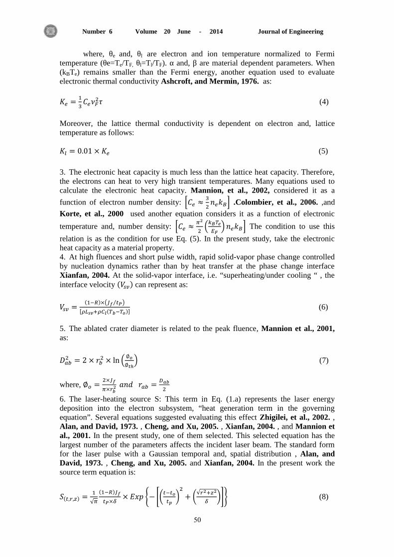
Journal of Engineering Volume 20 June - 2014 Number 6
75
where, θe and, θl are electron and ion temperature normalized to Fermi
temperature (θe=Te/TF, θl=Tl/TF). α and, β are material dependent parameters. When
(kBTe) remains smaller than the Fermi energy, another equation used to evaluate
electronic thermal conductivity Ashcroft, and Mermin, 1976. as:
(4)
Moreover, the lattice thermal conductivity is dependent on electron and, lattice
temperature as follows:
(5)
3. The electronic heat capacity is much less than the lattice heat capacity. Therefore,
the electrons can heat to very high transient temperatures. Many equations used to
calculate the electronic heat capacity. Mannion, et al., 2002, considered it as a
function of electron number density: *
+ .Colombier, et al., 2006. ,and
Korte, et al., 2000 used another equation considers it as a function of electronic
temperature and, number density: *
(
) + The condition to use this
relation is as the condition for use Eq. (5). In the present study, take the electronic
heat capacity as a material property.
4. At high fluences and short pulse width, rapid solid-vapor phase change controlled
by nucleation dynamics rather than by heat transfer at the phase change interface
Xianfan, 2004. At the solid-vapor interface, i.e. “superheating/under cooling “ , the
interface velocity ( ) can represent as:
( ) ( ⁄ )
[ ( )] (6)
5. The ablated crater diameter is related to the peak fluence, Mannion et al., 2001,
as:
(
) (7)
where,
6. The laser-heating source S: This term in Eq. (1.a) represents the laser energy
deposition into the electron subsystem, “heat generation term in the governing
equation”. Several equations suggested evaluating this effect Zhigilei, et al., 2002. ,
Alan, and David, 1973. , Cheng, and Xu, 2005. , Xianfan, 2004. , and Mannion et
al., 2001. In the present study, one of them selected. This selected equation has the
largest number of the parameters affects the incident laser beam. The standard form
for the laser pulse with a Gaussian temporal and, spatial distribution , Alan, and
David, 1973. , Cheng, and Xu, 2005. and Xianfan, 2004. In the present work the
source term equation is:
( )
√
( )
{ [(
)
(√
)]} (8)

Journal of Engineering Volume 20 June - 2014 Number 6
75
As indicated before, Alan, and David, 1973, showed that when the cylinder is
solid rather than hollow. The third term in the R.H.S of Eq. (1) becomes:
(
) (
) (
) (
) ⁄ (
) (
) ⁄ (9)
Therefore, Eq. (1) can be written as:
(
) (
) ( ) (10.a)
(
) (
) ( ) (10.b)
Where z is measured along the axis of ejection of the plasma and r radial
outwards from the axis. A special consideration must be given to the central node at
0r . At 0r the first term in the R.H.S of Eq. (10),(
) (
) is indeterminate. This
term can be evaluated by suing L'Hopital's rule.
(
) (
) ,(
) (
) (
) ( )⁄ - (
) (11)
Thus the governing Eq. (10) can be re-formulated as:
(
) (
) ( ) (12.a)
(
) (
) ( ) (12.b)
2. 2. Initial and Boundary conditions
Applying initial and boundary conditions to solves Eq. (12). The electron and
lattice initial temperature of the material target equal the ambient temperature. Yet
there is no laser beam incident on the material surface Schäfer, et al., 2002.
At ( ) (13.a)
( ) (13.b)
The mechanism for machining with femtosecond laser pulse is very different
from the conventional laser machining. Where the pulse duration small and, there is
no enough time for convection and radiation losses. In other words, no heat will
release from the upper boundary of the target, see Fig. 1.a.
At ( )
| (14.a)
( )
|
(14.b)

Journal of Engineering Volume 20 June - 2014 Number 6
75
Select the origin point of the domain into, the center of the upper surface of
the target, from symmetry of the cylindrical geometry. The boundary conditions
obtained as follows:
At ( )
| (15.a)
( )
|
(15.b)
The nature of the femtosecond laser ablation is different. Therefore, diffusion
effect is very little in comparison with the conventional mechanisms. As a result, that
the bottom surface of the material target considered insulated Alan, and David, 1973.
These words also right for the distance far in the radial direction.
At ( )
| (16.a)
( )
| (16.b)
At ( )
| (17.a)
( )
| (17.b)
3. NUMERICAL SOLUTION
A numerical solution of Eq. (12) depends upon the explicit finite difference
technique to calculate the electron and lattice temperature distribution of plume
through r and z axes. The scripts T and F used for the electron and lattice
temperatures respectively, then the indices i and j will be used for indicating the
points along the r and z directions respectively, and the index n will be used for
indicating the points over the time layers. We shall use the approximation of the first
order of accuracy for time, and of the second order of accuracy for space. The
distances between the points in the established grid are tandzr ,, .The grid is
represented by Fig. 1.c. The finite difference form of Eq.(12) with explicit
formulation, Anderson, et al., 1984. :
For electron subsystem:
(
)
(
)
(
)
(18.a)
For lattice subsystem
(
)
(
)
(
)
(
)
(
)
(18.b)

Journal of Engineering Volume 20 June - 2014 Number 6
75
The Eq. (18) is so-called explicit formulation of Eq. (12). Then after
applying the boundary conditions, the governing equation for every zone in the
solution domain is:
1. At 0r and 0z . n
ji
n
ji TT ,1,1 and n
ji
n
ji FF ,1,1 and n
ji
n
ji TT 1,1, and
n
ji
n
ji FF 1,1, Eq. (18) can be re-written in the central difference form as:
(
)
(
)
( )
(19.a)
(
)
(
)
(
)
(19.b)
2. At Lr0 and 0z . n
ji
n
ji TT 1,1, and n
ji
n
ji FF 1,1, Eqns. (18) can be re-written
in the central difference form as:
(
)
(
)
(
)
(
)
(20.a)
(
)
(
)
(
)
(
)
(20.b)
3. At 0r and Lz0 . n
ji
n
ji TT ,1,1 and n
ji
n
ji FF ,1,1 Eq. (18) can be re-written in
the central difference form as:
(
)
(
)
(
)
(21.a)
(
)
(
)
(
)
(
)
(21.b)
4. Apply Eqns. (18) when
.
(
) Is the convergence term as described by references, Alan,
and David, 1973. , and Anderson, et al., 1984. Where the convergence criteria
mentioned that the value of the convergence term must be greater than or equal zero,
to avoid solution fluctuation:
The electron and lattice temperature distribution through r-z plane, where
2r to 1L and 2z to 1L is represented as shown in Fig. 1.b. A special

Journal of Engineering Volume 20 June - 2014 Number 6
76
consideration is carried out for the exterior nods, with aid of factious points to mesh.
The computer program was built in Visual FORTRAN language and run on pentium4
PC, using operating system Microsoft XP. Run time of about several minutes was
needed to achieve the required convergence.
4. REULTES AND DISCUSSION
Figs. 2 to 5 explain the electron and lattice subsystem reduced temperature
temporal distribution through the time with respect to laser pulse duration. Form these
figures can be conclude that the temperature of the electron subsystem raised rapidly
and approached to peak value at the end of laser pulse duration because of that the
electron heat capacity is less than the lattice heat capacity. Electrons absorb the laser
energy i.e., where the free electrons absorb the incident energy of the laser pulse due
to invers-Bremsstrahlnug Grojo, et al., 2003 and Zeng, and Xianzhong, 2004. In
addition the electron heat capacity is low in comparison with the lattice-subsystem
heat capacity, Mannion, et al., 2001. At the end of the pulse duration the temperature
of the electron subsystem will decrease rapidly sometimes suddenly due to the
electron-phonon (lattice) coupling and energy transfer to the lattice subsystem, as
shown in Figs. 4 and 5.
In accordance with the different in the heat capacities of electron and lattice
subsystems, the lattice temperature subsystem not much increase in compared with
the electron subsystem. Briefly the behavior of electron and lattice can be expressed
as the electron temperature will be increased rapidly until the end of laser pulse, then
decreased rapidly. Moreover for the lattice subsystem, the temperature profile
increased slowly form the beginning of laser pulse and remain increased after the end
of pulse duration (for several pulse duration times), due to large heat capacity for the
lattice subsystem, Cheng, and Xu, 2005.
The electron temperature reaches peak value at the end of laser pulse. It can
also be seen that till this time the lattice remains virtually cold. Subsequently, the
initial laser energy is totally absorbed by the electrons within the optical penetration
depth. These energetic electrons move at very high speeds on the order of ~ 106 m/s.
Subsequently, the electrons reach thermal equilibrium and diffuse deeper into the
material at reduced speeds. It is only at a much longer time scale that energy transfer
to the lattice occurs. Thereafter, both the electrons and the lattice reach the same
temperature, and at long time scales > 40 ps they behave as a single system. Beyond
this time, heat transfer occurs by conduction at much lower speeds, Chimmalgi, et
al., 2005. Therefore, it can be stated that the calculations consistence with the
published results.
In comparison between Figs. 2, 3 for nickel and Figs. 4, 5 for copper, it can be
noticed that the reduced temperature profile for electron subsystem of copper metal is
suddenly decreased after pulse duration due to electron-phonon relaxation coupling.
Figs. 6 and 7 show the electron and lattice subsystems reduced temperature
profiles (T/TC) versus the reduced radius (r/R) at time (1 tp), "the end of laser pulse".
These figures indicate that the electron and lattice temperatures reach the peak value
at the center of the laser crater because of Gaussian distribution of the laser beam. In
addition, the value of the electron temperature is much higher than the lattice
temperature for the same reasons as in Figs. 2 to 5.
Figs. 8 and 9 explain the electron and lattice subsystems reduced temperature
(T/TC) versus the reduced depth (z/R) at the end of pulse. These figures show that in
spite of that the free electrons in the surface layer of target metal absorbs the laser
beam energy, that the free electrons in the depth of metal target are also absorbs the

Journal of Engineering Volume 20 June - 2014 Number 6
77
energy of the transmitted part of the irradiated beam. Finally, the energy of the
electron subsystem is transferred to lattice subsystem; after several times of pulse
duration. In addition, that the reduced temperature profile will be decreased gradually
with depth. Finally the temperature profile for the electron and lattice subsystems will
be approached the same value at the distance far from the surface of the metal target.
At different pulse duration times, Figs. 10 and 12 indicate the spatial
temperature distribution for electron subsystem. The temperature curve for every
figure show that the temperature increased with time and reached the maximum value
at time equals 1 tp, and then the temperature will be decreased rapidly and approached
initial value after several tp. It can be noticed that the temperature profile in the radial
and depth direction approximately the same.
Figs. 11 and 13 show the distribution of reduced lattice temperature spatially
for different pulse duration times in the radial and depth directions. From these
figures, it can be noticed that the reduced temperature levels is less than the reduced
temperature values in Figs. 10 and 12 respectively, where the heat capacity of lattice
subsystem is greater than that of electron subsystem, Qiu, & Tien, 1993. The reduced
lattice temperature approaches the peak value at time equals 5 tp. In comparison with
Figs. 10 and 12, it can be concluded that the lattice subsystem gain the heat slowly,
but the free electrons absorb heat rapidly and radiant it at high rate.
Figs. 14 and 15 plot the isothermal contour map for reduced electron and
lattice temperature in the rz-plane for copper. These two figures indicate the big
difference in the temperature levels between the free electron and lattice subsystem,
for the same conditions.
5. CONCLUSION
The time evolution for temperature of electron subsystem is faster than the
temperature of lattice subsystem. Where, the heat capacity of the lattice was higher
than the heat capacity of the free electrons. The metal target treated as two
subsystems, in the ultra-short pulsed laser irradiation. The plasma plume existence in
the ultra-short pulsed laser where, the temperatures of the electron and lattice
subsystems exceed the critical temperature.
The weaker non-equilibrium between the electron and lattice (phonon) during
the laser pulse reduce the ablation rate, and vies versa especially for Nickel. Nickel
has a shorter lattice response time than for the copper. As explained in Figs. 2 to 5.
As a rule, the models employed in the theory of laser ablation are reliant on
complex nonlinear systems of partial differential equations whose solution calls for
the use of numerical methods.

Journal of Engineering Volume 20 June - 2014 Number 6
78
Figure 1. Type of fixed boundary conditions for electron and
lattice temperature distributions.
Δr
Δz
i,j i+1,j i-1,j
i,j+1
i,j-1
z
r
(b) (c)
Gird point interval in space difference
Gird point interval in time difference
si
tn
Δt
Δs
tn+1
s i+1 s
i-1
θ
z
r
Laser Beam
(a) Schematic of the computational domain

Journal of Engineering Volume 20 June - 2014 Number 6
79
: :
0.00 0.25 0.50 0.75 1.00 1.25 1.50 1.75 2.00
(time/tp) reduced time
0.00
0.25
0.50
0.75
1.00
1.25(T
/Tc)
red
uce
d t
em
per
ature
electron temp.
lattice temp.
Figure(2) Reduced lattice & electron temp. vs. the pulse duration time for tp=0.5E-12 sec
Jf=0.27 J/cm metal:Nickel
0.00 0.25 0.50 0.75 1.00 1.25 1.50 1.75 2.00
(time/tp) reduced time
0.0
0.5
1.0
1.5
2.0
2.5
3.0
3.5
4.0
4.5
(T/T
c) r
educe
d t
em
per
ature
electron temp.
lattice temp.
Figure(3) Reduced lattice & electron temp. vs.
the pulse duration time for tp=0.5E-12 sec
Jf=1.0 J/cm metal:Nickel
0.00 0.25 0.50 0.75 1.00 1.25 1.50 1.75 2.00
(time/tp) reduced time
0.0
0.5
1.0
1.5
2.0
2.5
3.0
3.5
4.0
4.5
5.0(T
/Tc)
red
uce
d t
em
per
ature
electron temp.
lattice temp.
Figure(5) Reduced lattice & electron temp.vs.
the pulse duration time for tp=0.5E-12 sec
Jf=1.0 W/cm Metal:Copper
0.00 0.25 0.50 0.75 1.00 1.25 1.50 1.75 2.00
(time/tp) reduced time
0.0
0.2
0.4
0.6
0.8
1.0
1.2
1.4
1.6
(T/T
c) r
educe
d t
em
per
ature
electron temp.
lattice temp.
Figure(4) Reduced lattice & electron temp.vs.
the pulse duration time for tp=0.5E-12 sec
Jf=0.3529 J/cm Metal:Copper
0.0 0.2 0.4 0.6 0.8 1.0(r/R) reduced raduis
0.00
0.25
0.50
0.75
1.00
1.25
(T/T
c) r
educe
d t
emper
atu
re at time=1 tp
electron temp.
lattice temp.
Figure(6) Reduced electron & lattice temp. vs.
reduced radial distance for tp=0.5E-12 sec
Jf=0.27 J/cm metal:Nickel
0.0 0.2 0.4 0.6 0.8 1.0(r/R) reduced raduis
0.0
0.2
0.4
0.6
0.8
1.0
1.2
1.4
1.6
(T/T
c) r
educe
d t
emper
atu
re at time=1 tp
electron temp.
lattice temp.
Figure(7) Reduced electron & lattice temp. vs.
reduced radial distance for tp=0.5E-12 sec
Jf=0.3529 J/cm metal:Copper
2 2
: :
: :
Figure 2. Reduced Lattice & Electron
Temp. vs. the Pulse Duration Time for
tp=0.5E-12 S, Jf=0.27 J/cm2 Metal:Nickel
Figure 3. Reduced Lattice & Electron
Temp. vs. the Pulse Duration Time for
tp=0.5E-12 S, Jf=1.0 J/cm2 Metal:Nickel
Figure 4. Reduced Lattice & Electron Temp.
vs. the Pulse Duration Time for tp=0.5E-12 S,
Jf=0.3529 J/cm2 Metal:Copper
Figure 5. Reduced Lattice & Electron
Temp. vs. the Pulse Duration Time for
tp=0.5E-12 S, Jf=1.0 J/cm2 Metal:Copper
Figure 6. Reduced Lattice & Electron
Temp. vs. Radial Dist for tp=0.5E-12 S,
Jf=0.27 J/cm2 Metal:Nickel
Figure 7. Reduced Lattice & Electron
Temp. vs. Radial Dist. for tp=0.5E-12 S,
Jf=0.3529 J/cm2 Metal:Copper

Journal of Engineering Volume 20 June - 2014 Number 6
7:
:
:
:
0.0 0.2 0.4 0.6 0.8 1.0
(z/R) reduced depth
0.00
0.25
0.50
0.75
1.00
1.25(T
/Tc)
reduced t
em
pera
ture
at time=1 tp
electron temp.
lattice temp.
Figure(8) Reduced electron & lattice temp.vs.
reduced depth distance for tp=0.5E-12 sec
Jf=0.27 J/cm metal:Nickel
0.0 0.2 0.4 0.6 0.8 1.0(z/R) reduced depth
0.0
0.2
0.4
0.6
0.8
1.0
1.2
1.4
1.6
(T/T
c)
reduced t
em
pera
ture at time=1 tp
electron temp.
lattice temp.
Figure(9) Reduced electron & lattice temp.vs.
reduced depth distance for tp=0.5E-12 sec
Jf=0.3529 J/cm metal:Copper
0.0 0.2 0.4 0.6 0.8 1.0
(r/R) reduced radius
0.0
0.6
1.2
1.8
2.4
3.0
3.6
4.2
4.8
(T/T
c)
reduced e
lectr
on t
em
p. time in tp
time=0 tp
time=0.5 tp
time=1 tp
time=5 tp
time=10 tp
Figure(10) Reduced electron temp. for differet pulse
duration times vs. reduced raduis for
tp=0.5E-12 sec Jf=1.0 J/cm metal:Nickel
0.0 0.2 0.4 0.6 0.8 1.0
(z/R) reduced depth
0.0
0.6
1.2
1.8
2.4
3.0
3.6
4.2
4.8
(T/T
c)
reduced t
em
p.
time in tp
time=0 tp
time=0.5 tp
time=1 tp
time=5 tp
time=10 tp
Figure(12) Reduced electron temp. for different pulse
duration times vs. reduced depth for
tp=0.5E-12 sec Jf=1.0 J/cm metal:Nickel
0.0 0.2 0.4 0.6 0.8 1.0
(z/R) reduced depth
0.00
0.05
0.10
0.15
0.20
0.25
0.30
(T/T
c)
reduced t
em
p.
time in tp
time=0 tp
time=0.5 tp
time=1 tp
time=5 tp
time=10 tp
Figure(13) Reduced lattice temp. for different pulse
duration times vs. reduced depth for
tp=0.5E-12 sec Jf=1.0 J/cm metal:Nickel
0.0 0.2 0.4 0.6 0.8 1.0(r/R) reduced radius
0.00
0.05
0.10
0.15
0.20
0.25
0.30
(T/T
c)
reduced e
lectr
on t
em
p. time in tp
time=0 tp
time=0.5 tp
time=1 tp
time=5 tp
time=10 tp
Figure(11) Reduced lattice temp. for different pulse
duration times vs. reduced raduis for
tp=0.5E-12 sec Jf=1.0 J/cm metal:Nickel
:
:
:
Figure 8. Reduced Lattice & Electron
Temp. vs. Reduced Depth Dist. for
tp=0.5E-12 S, Jf=0.27 J/cm2 Metal:Nickel
Figure 9. Reduced Lattice & Electron Temp.
vs. Reduced Depth Dist. for tp=0.5E-12 S,
Jf=0.3529 J/cm2 Metal:Copper
Figure 10. Reduced Electron Temp. for Different
Pulse Duration Times vs. Reduced Raduis for
tp=0.5E-12 S, Jf=0.3529 J/cm2 Metal:Nickel
Figure 11. Reduced Lattice Temp. for Different
Pulse Duration Times vs. Reduced Raduis for
tp=0.5E-12 S, Jf=1.0 J/cm2 Metal:Nickel
Figure 12. Reduced Electron Temp. for Different
Pulse Duration Times vs. Reduced Depth for
tp=0.5E-12 S, Jf=1.0 J/cm2 Metal:Nickel
Figure 13. Reduced Lattice Temp. for Different
Pulse Duration Times vs. Reduced Depth for
tp=0.5E-12 S, Jf=1.0 J/cm2 Metal:Nickel

Journal of Engineering Volume 20 June - 2014 Number 6
7;
0.000.050.100.150.20
(r/R)
0.00
0.05
0.10
0.15
0.20
(z/R
)
0.0
0.5
1.0
1.5
2.0
2.5
3.0
3.5
4.0
4.5
5.0
Figure(14) Isothermal contour map of reduced electron temp.vs. the normlized rz-plane for tp=0.5E-12 sec Jf=1.0 J/cm metal:Copper
0.000.050.100.150.20
(r/R)
0.00
0.05
0.10
0.15
0.20
(z/R
)
0.06
0.12
0.18
0.24
0.30
0.36
Figure(15) Isothermal contour map of reduced lattice temp.vs. thenormlized rz-plane for tp=0.5E-12 sec Jf=1.0 J/cm metal:Copper
:
:
r-z palne
r-z palne

Journal of Engineering Volume 20 June - 2014 Number 6
85
NOMENCLATURES
Sample Description Unite
specific heat of electron subsystem J/m3.K specific heat of lattice subsystem J/m3.K electron diffusion coefficient m2/S energy transferred J fermi energy J subscript denotes the electron subsystem -- subscript denotes the lattice subsystem -- laser power intensity W/cm2 The indexes increase along the r, z --
incident laser fluence W/m2 electron thermal conductivity coefficient W/m.K lattice thermal conductivity coefficient W/m.K Boltzmann constant enthalpy of sublimation per atom J/kg electron mass kg electron density m-3 index increases along the time -- material reflectivity -- radial distance m radius of ablation crater m source in the governing equation S time S laser pulse duration time S electron temperature K electron temperature in numerical form K lattice temperature K lattice temperature in numerical form K Fermi temperature K ambient temperature K boiling temperature K critical temperature K solid-vapor interface velocity m/S material dependent parameter --
material density Kg/m3 electron relaxation time which is determined by electron-
electron and electron-phonon collisions. S
coefficient of electron-lattice relaxation rate W/m3.K electron velocity m/S absorption ablation depth m

Journal of Engineering Volume 20 June - 2014 Number 6
85
REFERENCES
Al-moosawy, Adil, A., 2002, Modeling of Thermal History of Solid Material
Processed by Laser , Ph.D. Thesis, University of Technology, Mech. Dept.,.
Alan Adams, J., and David, F., Rogers., 1973, Computer-Aided Heat Transfer
Analysis, McGraw-Hill,.
Anderson, D. A., Tannehill, J. C., and Pletcher, R. H., 1984, Computational Fluid
Mechanics and Heat Transfer, McGraw-Hill,.
Bulgakova, M., Nadezhda, M., Igor, Burakov, Meshcherykov, Yuri, P., Stoian,
Razvan, Rosenfeld, Arkadi, and Hertel, Ingolf, V., 2007,Theoretical Models and
Qualitative Interpretations of Fs Laser Material Processing, JLMN-Journal of
Laser Micro/Nanoengineering Vol. 2, No. 1,.
Chimmalgi, A., Grigoropoulos, C., P., and Komvopoulos, K., 2005, Surface
Nanostructuring by Nano-femtosecond Laser-assisted Scanning Force Microscopy,
Journal of Applied Physics, 97, 104319.
Cheng, Changrui, and Xu, Xianfan, 2005, Mechanisms of Decomposition of Metal
during Femtosecond Laser Ablation, Physical Review B,72,165415,.
Grojo, D., Hermann, J., Bruneau, S., and Itina, T., 2003, Analyses of Femtosecond
Laser Ablation of Ti, Zr and Hf, LP3-FRE 2165 CNRS,Faculté des Sciences de
Luminy,Case 917,13288 Marseille Cedex 9,France.
Hermann, J., Benfarah, M., Coustillier, G., Bruneau, S., Axente, E., Guillemoles, J.,-
F., Sentis, M., Alloncle, P., Itina, T., 2005, Selective Ablation of Thin Films with
Short and Ultrashort Laser Pulses, Applied Surface Science.
Harrach, R. J., Dec. 1977, Analyatic Solutions for Laser Heating and Burn-through of
Opaque Slabs, J. Appl. Phys., Vol. 48, pp. 2370-2375.
J.P. Colombier, P. Combis, F. Bonneau, R. Le Harzic, and E. Audouard., 2006,
Hydrodynamic Simulations of Metal Ablation by Femtosecond Laser Irradiation,
Dept. de Physique Th´eorique et Appliqu´ee ,France.
Korte, F. Adams S., Egbert, A. Fallnich, C. Ostendorf, A., 17July, 2000, Sub-
diffraction Limited Structuring of Solid Targets with Femtosecond Laser Pulses,
Institute of Applied Physics, Friedrich-Schiller-University Jena, Vol.7,
No.2/Optics Express,Jena,Germany.
Leitz, Karl-Heinz, Redlingshöfer, Benjamin, Reg, Yvonne, Otto, Andreas, Schmidt,
Michael, 2011, Metal Ablation with Short and Ultrashort Laser Pulses, Physics
Procedia 12, 230‒238.
Mannion, P. T., Favre, S., Mullan, C., Ivanov, D. S., O'Connor, G. M., Glynn, T. J.,
Doggett, B., and, Lunney, J. G., 2002, Langmuir Probe Investigation of Plasma

Journal of Engineering Volume 20 June - 2014 Number 6
85
Expansion in Femto and Picosecond Laser Ablation of Selected Metals ,National
Centre for Laser Applications, NUI Galway, Ireland.
Mannion, Paul, Magee, Jonathan, Coyne, Edward, and M., O’Connor, Gerard, 2001,
Ablation Thresholds in Ultrafast Laser Micro-machining of Common Metals in
Air, National Centre for Laser Applications, National University of Ireland,
Galway, Ireland, Proc. of SPIE Vol. 4876.
N.W. Ashcroft and N.D. Mermin, Solid State Physics ,Saunders College Publishing,
New York,1976.
Qiu, T. Q., and Tien, C. L., 1993, Heat Transfer Mechanisms During Short-pulse
Laser Heating of Metals ASME J. Heat Transfer, 115, pp. 835‒841.
Schäfer, C.; Urbassek, H.M.; Zhigilei, L.V., 2002,Metal Ablation by Picosecond
Laser Pulses: A hybrid simulation. Phys. Rev. B, in press.
S.I. Anisimov, B.S. Luk’yanchuk, A. Luches, 1996, An Analytical Model for Three-
dimensional Laser Plume Expansion into Vacuum in Hydrodynamic Regime, Appl.
Surface Science 96-98, pp 24-32.
S.I. Anisimov and B. Rethfeld, Izv. Ross. Akad. Nauk, Ser. Fiz. 61, 1642, 1997.
Xianfan Xu , 2004, Molecular Dynamics Study of Phase Change Mechanisms During
Femtosecond Laser Ablation, Journal of Heat Transfer (ASME).
Zhigilei, Leonid, V., and Dongare, Avinash, M., 2002, Multi-scale Modeling of Laser
Ablation: Applications to Nanotechnology, CMES, vol.3, no.5, pp.539-555,
Zeng, Xianzhong, 2004,Laser Ablation of Electronic Materials Including the Effects
of Energy Coupling and Plasma Interactions, Ph.D. Thesis, University of
California, Berkeley.

Journal of Engineering Volume 20 June - 2014 Number 6
63
Energy Savings in Thermal Insulations for Sustainable Buildings
Prof.Dr. Angham Alsaffar Qusay Adnan Alwan
Department of Civil Engineering Department of Civil Engineering
Collage of Engineering Collage of Engineering
Baghdad University Baghdad University
Email: [email protected] Email: [email protected]
ABSTRACT
Energy use is second to staffing in building operating costs. Sustainable technology in the
energy sector is based on utilizing renewable sources of energy such as solar, wind, glazing systems,
insulation. Other areas of focus include heating, ventilation and air conditioning; novel materials and
construction methods; improved sensors and monitoring systems; and advanced simulation tools that
can help building designers make more energy efficient choices.
The objective of this research is studying the effect of insulations on energy consumption of
buildings in Iraq and identifying the amount of energy savings from application the insulations in
buildings. HAP (Hourly Analysis Program) is used to calculate the thermal loads and the amount of
energy needed. It is concluded that the use of the thermal insulation in the roof, walls, floors, and
double glazing system for windows in building effectively reduces the energy required for air
conditioning.
Keywords: sustainable buildings design, energy efficiency technologies, insulations, double glazing
system.
مستذامةال وفورات الطاقة في العزل الحراري لالبنية
قصي عذنان علوان نغام الصفارأأ.د.
قسى انهذسخ انذيخ قسى انهذسخ انذيخ
خبيعخ ثغذاد/كهيخ انهذسخ خبيعخ ثغذاد/كهيخ انهذسخ
الخالصة
ان انطبقخ قطبع في انستذايخ انتكىنىخيب تستذ. انجتكبنيف تشغيم في انثبيخ انشتجخفي انطبقخ استخذاو يبتي
،انتذفئخ تتض أخشي يدبالدهبك . انعضلو انضخبج، أظخ انشيبذ،طبقخ ،انطبقخ انشسيخ يثم انتدذدح انطبقخ يصبدس استخذاو
انتطىسح انحبكبح وأدواد انشصذ، وظى االستشعبس أخهضح وتحسي ، خذيذح يىاداستخذاو وانجبء أسبنيت انهىاء، وتكييف انتهىيخ
.كثش كابءحاالانطبقخ اختيبسفي انج يصي تسبعذ أ يك
ثيخدساسخ تبثيش انعىاصل في اندذسا وانسقىف واالسضيبد وانىافز عه استهالك انطبقخ في اال انهزا انجحث يهذف
Hourly Analysisاستخذاو ثشبيح تى .ثيخي تطجيق انعىاصل في اال هوتحذيذ كيخ انىفىساد في انطبقخ انبتد في انعشاق
Program نحسبة االحبل انحشاسيخ وكيخ انطبقخ انالصيخ. حيث تجي ا استخذاو انعبصل في اندذسا واالسضيبد وانسقىف
.ي كيخ انطبقخ انالصيخ نهتكييف ثشكم فعبل يقهم في االثيخ واستخذاو انىافز راد انضخبج انضدصج
.ظبو انضخبج انضدوج انعىاصل، ،تقيبد كابءح انطبقخ ،تصيى االثيخ انستذاو كلمات رئيسية:

Journal of Engineering Volume 20 June - 2014 Number 6
64
1. INTRODUCTION
Sustainable design, green architecture, sustainable constructions, and green buildings these
are all new way and method for designing and constructing. The environmental and economical
challenges of this era are affecting many sectors. New buildings are being designed, executed and
operated by modern technologies which reduces the environmental impact and at the same time
leads to reduction in cost especially running costs. Buildings are large consumers of energy in all countries. In regions with harsh climatic
conditions, a substantial share of energy goes to heat and cool buildings. This heating and air-
conditioning load can be reduced through many means; notable among them is the proper design
and selection of building envelope and its components.
The proper use of thermal insulation in buildings does not only contribute in reducing the
required air-conditioning system size but also in reducing the annual energy cost. Additionally, it
helps in extending the periods of thermal comfort without reliance on mechanical air-conditioning
especially during inter-seasons periods. The magnitude of energy savings as a result of using
thermal insulation vary according to the building type, the climatic conditions at which the building
is located as well as the type of the insulating material used. The question now in the minds of many
building owners is no longer should insulation be used but rather which type, how, and how much.
2. RESEARCH OBJECTIVE
The objective of this research is to identify the potential savings in energy for Building by
using insulations in walls, floors, roof, and windows. In order to calculate the energy savings in
building, HAP 4.7 (Hourly Analysis Program) from Carrier is used to calculate the thermal loads on
two stages:
1. Building without insulations.
2. Building with insulations.
The main objectives of this research are:
1. Identifying the potential quantitative savings in energy from the application of insulations in
green house.
2. Studying the effect of sustainable energy technologies systems in Buildings.
3. SUSTAINABILITY
The concept of sustainability in building and construction has evolved over many years. The
initial focus was on how to deal with the issue of limited resources. More recently, an appreciation
of the significance of non-technical issues has grown. It is now recognized that economic and social
sustainability are important, as are the cultural heritage aspects of the built environment. Sustainable
design concept can be divided into following aspects, Jain et al., 2013:
1. Sustainable site planning, preservation of site character, erosion, and sedimentation.
Buildings envelop design, optimum design as per climate conditions and energy
conservation building codes.
2. Ecologically sustainable material which is based on zero or low toxicity reduces adverse
environmental impact.
3. Indoor Ambience, ventilation system to meet minimum indoor air ventilation rates.

Journal of Engineering Volume 20 June - 2014 Number 6
65
.
4. Water and waste management, facilitate efficiency in use of water resources.
5. Integration of renewable energy use of energy efficient fixture, materials and integration of
energy sources.
4. ENERGY EFFICIENCY TECHNOLOGIES Energy needs can be reduced in several ways. Improving the performance of a building's
envelope means less heating and cooling energy will be required, so the Heating, Ventilation, and
Air Conditioning (HVAC) system can be smaller. High efficiency motors should be specified for all
heating, ventilation, and air Conditioning components and heat recovery systems. More efficient
lighting designs will reduce both lighting and cooling energy costs ,Perkins and Stantec, 2003.
4.1 Glazing System
Double glazing window system is commonly used in buildings of today. There have been
many attempts to improve the insulation performance of this system such as low-e coating of glass
surface, gas-filling between the glass panes, inserting a thermal breaker made of polyurethane or
polyamide in frame, etc.. ,Song et al., 2005.
The performance of glazing is dependent on the overall rate of heat flow (U-value or thermal
transmittance), Solar Heat Gain Coefficient, and visible transmittance. The U-Factor is a measure of
how easily heat is transferred through a material and therefore a lower U-Factor indicates the lower
amount of heat transfer through a window (from the interior to the exterior). The Solar Heat Gain
Coefficient (SHGC) is the fraction of solar heat that enters through a glazing system and becomes
heat. Visible transmittance (VT) is the percentage of the visible spectrum that is transmitted through
glazing. For example, when daylight is a desired goal, glazing with a high VT is preferable ,Perkins
and Stantec, 2003.
Double-glazing can substantially reduce the U-value of the glazed area of a building and as
such it has become popular. However, double-glazing units are composed of a number of
components as opposed to single sheets of glass. Double-glazing units are composed of a number of
different materials, including glass, spacer bar, desiccant and sealant. The ultimate properties,
qualities and Life time of any double-glazing units depends to a large extent on the type and quality
of the individual components and the excellence of their manufacture, Garvin and Wilson, 1998.
In the UK the majority of PVC-U and aluminum frames are drained and ventilated.
However, timber and steel windows are more commonly fully bedded. Examples of both types of
system are shown in Fig. 1 and Fig. 2, Garvin and Wilson, 1998.
4.2 Insulation
Well-insulated building envelopes are primary considerations in comfort and sustainability.
Insulation helps to protect a building’s occupants from heat, cold, and noise; in addition, it reduces
pollution while conserving the energy needed to heat and cool a building. The comfort and energy
efficiency of a home and, to a lesser degree, an office depend on the thermal resistance (R value) of
the entire wall, roof, or floor (i.e., whole-wall R value), not just the R-value of the insulation.
Techniques such as advanced framing increase the wall area covered by insulation, thereby
increasing the whole wall’s effectiveness. Framing conducts far more heat than insulation, in the
same manner that most window frames conduct more heat than double-paned glass. An additional

Journal of Engineering Volume 20 June - 2014 Number 6
66
layer of rigid insulation between framing and exterior sheathing can help improve the whole-wall
R-value by insulating the entire wall, and not just the clear space,Kubba, 2009.
According to Mohsen and Akash,2001, the heating load was calculated for a typical single
house using different insulation materials. It was shown that the energy saving up to 77% can be
achieved when polystyrene is used for both wall and roof insulation. Al-Homoud, 2004, summarized the benefits for using thermal insulation in buildings, as follows:
1. A matter of principle: Using thermal insulation in buildings helps in reducing the reliance on
mechanical/electrical systems to operate buildings comfortably and, therefore, conserves
energy and the associated natural resources.
2. Economic benefits: An energy cost is an operating cost, and great energy savings can be
achieved by using thermal insulation.
3. Environmental benefits: The use of thermal insulation.
4. Thermally comfortable buildings: The use of thermal insulation in buildings extends the
periods of indoor thermal comfort especially in between seasons.
5. Reduced noise levels.
6. Building structural integrity.
7. Vapor condensation prevention: Proper design and installation of thermal insulation helps in
preventing vapor condensation on building surfaces.
8. Fire protection.
American Society of Heating, Refrigerating and Air Conditioning Engineers (2001)
mentioned building thermal insulation, which fall under the following basic materials and
composites:
1. Inorganic Materials
Fibrous materials such as glass, rock, and slag wool.
Cellular materials such as calcium silicate, bonded perlite, vermiculite, and ceramic
products.
2. Organic Materials
Fibrous materials such as cellulose, cotton, wood, pulp, cane, or synthetic fibers.
Cellular materials such as cork, foamed rubber, polystyrene, polyethylene, polyurethane,
polyisocy-anurate and other polymers.
3. Metallic or metalized reflective membranes: These must face an air-filled, gas-filled, or
evacuated space to be effective.
Fig. 3 shows a graphical comparison of the thermal resistances of 5 cm thickness for
common building insulation materials. Concrete block is not considered as an insulating
material. However, it was included in the figure as a reference (no insulation case) for
comparison purposes only.
5. CASE STUDY
The case study evaluates the impacts of high quality insulation in energy consumption in
single-family home. In this study a typical Iraqi house layout is considered for a single family. The
consists of two floors ground and first floor with a total plot area about 200 square meters having
four rooms and two bathrooms one in each floor.

Journal of Engineering Volume 20 June - 2014 Number 6
67
Assumptions:
Air conditioning system consists of package unit and all house walls, roofs and floors without
insulations in home.
1. Glass considered single layer with 4 mm thick for windows and doors.
2. The Air Conditioning (AC) plans layout shown in Fig. 4.
3. Air Conditioning work 7 months from (April to October).
4. Ordinary bricks used for non-insulated house and insulated concrete block used for insulated
house.
5.1 Energy Baseline Usage for Non-insulated House
In order to calculate the efficiency of the new technologies used for sustainable house
design, the baseline energy consumption of air conditioning use should be calculated.
Baseline energy consumption of the air condition of the house in the case that the house has
not used insulation in the walls, roofs and floors, and windows HAP 4.7 (Hourly Analysis Program)
from Carrier is used to calculate the thermal loads. So, What Is HAP?
Carrier's Hourly Analysis Program is two powerful tools in one package. HAP provides
versatile features for designing HVAC systems for commercial buildings. It also offers powerful
energy analysis capabilities for comparing energy consumption and operating costs of design
alternatives. By combining both tools in one package significant time savings are achieved. Input
data and results from system design calculations can be used directly in energy studies.
HAP is used to calculate the thermal loads and the amount of energy needed through the
introduction of country specific information such as climate, latitude and longitude, spaces
dimensions and materials used in walls, floors and roofs. Hap calculated thermal loads and provides
the equivalent of the amount of cooling by type of cooling plants used.
Enter the information for each space in the house such as the name of the space, floor area,
room lighting, the number of people, walls and windows areas of space exposed to sun radiation,
roof area if exposed to sun radiation as shown in Fig.5.
After completing the introduction of all information about spaces of house then choosing the
AC plant type and specifications required. HAP program analyzes and calculates the thermal loads
and the monthly amount of energy required for a period of 7 months in kilowatt. hour (kw.h) as
shown in Table 1. The results show that the total amount of energy for non-insulated house =24989 kw.
h/year.
5.2 Application of Insulation
Majority of insulation in buildings is for thermal purposes, the term also applies to acoustic
insulation, fire insulation, and impact insulation. Thermal insulation in buildings is an important
factor to achieving thermal comfort for its occupants. Insulation reduces unwanted heat loss or gain
and can decrease the energy demands of heating and cooling systems. It does not necessarily deal
with issues of adequate ventilation and may or may not affect the level of sound insulation. In a
narrow sense insulation can just refer to the insulation materials employed to slow heat loss, such
as: cellulose, glass wool, rock wool, polystyrene, urethane foam, vermiculite, perlite, wood fiber,
plant fiber (cannabis, flax, cotton, cork, etc.).

Journal of Engineering Volume 20 June - 2014 Number 6
68
For the purpose of insulation the home, insulated concrete block with polystyrene thick 10
inches used instead of ordinary bricks for walls with 0.5 inch gypsum plaster and 0.5 inch cement
plaster so the overall thermal transmittance (U-Value) become 0.085 British temperature units /
Fahrenheit x foot square x hour (Btu/ F ft
2 h). roofs consist of 0.5 inch gypsum plaster, 8 inches
concrete, 0.5 inch asphalt sheathing, 2 inches R7 board insulation, 4 inches sand and 1.5 inches
cement tiles so the overall U-Value become 0.06 Btu/ F ft2 h. Double glazing 1/4 inch grey
reflective outer glaze and 1/4 inch clear with 1/2 inch air space used for windows. Fig.6 shows the
roof, wall, floor, and windows layers.
When insulated the walls, roofs, floors and windows the thermal transmittance U-value
become less than from non-insulated be. Fig. 7 shows the U-Value for non-insulated wall and
Table 2 shows the U-Values calculated by HAP. After completing the introduction of all
information about insulated spaces of House then choose the Air Conditioning plant type and
specifications required. HAP program analyzes and calculates the thermal loads and the monthly
amount of energy required for a period of 7 months in (kW.h) (see Table 3).
The results show the total amount of energy for insulated house =16874 kW.h/year Yearly
Savings of air conditioning will be 24989 ‒ 16874 = 8115 kW.hr/year
6. CONCLUSION The following points have been identified as the overall conclusions of the research:
1. The Sustainable design should seek to reduce negative impacts on the environment, and the
health and comfort of building occupants, thereby improving building performance.
Integration of architecture and technology can alleviate sustainability in a great way.
2. The cost of such green buildings may be higher by 5-10% than that of conventional building,
it will result in 30-40% energy saving and the excess cost can be recovered within 3-4 years.
The incorporation of sustainable features should be made mandatory through separate Bye
laws for energy efficient buildings to conserve depleting resources and to reduce the overall
negative impact of development on the environment.
3. Wall and roof insulation are recommended for buildings in all climates for more thermally
comfortable space and, therefore, less energy requirements. Insulation helps in reducing
conduction losses through all components of the building envelope. However, roof insulation
is generally more critical than walls and should be given more attention.
4. The use of the thermal insulation of the roof, walls, floors, and double glazing system for
windows effectively reduces the energy required for air conditioning can arrive where
rationalization in energy consumption to about 32%.
7. RECOMMENDATIONS
1. Sectors of urban planning and environment in Iraq must be responsible to develop a national
environmental strategy within the concept of sustainable development and issuance of new
laws to construction by participation of the planning departments of cities and municipalities
in the provinces and the implementation of these strategies during the next stage.
2. Proper treatment of building envelopes can significantly improve thermal performance
especially for envelope-load dominated buildings, such as residences. Therefore, the proper
selection and treatment of the building envelope components can significantly improve its
thermal performance.

Journal of Engineering Volume 20 June - 2014 Number 6
69
3. Designer is important joint in the development of the project in order to defend their own
ideas, to clarify the reasons, high-performance projects.
4. Legislation of Determinants relating to the use of renewable energy systems in buildings and
urban communities and modify construction systems to include special legislation to energy-
saving systems.
REFERENCES
AL-Homoud, M, S., 2004, Performance Characteristics and Practical Applications of Common
Building Thermal Insulation Materials, Journal: Building and Environment, Vol. 40, No. 3, p.p.
353-366.
American Society of Heating, Refrigerating, and Air Conditioning Engineers (ASHRAE), 2001,
Handbook of Fundamentals, Chapter 23, USA.
Perkins and Stantec, 2003 ,Sustainable Building Design Principles, Practices & Systems: A
Study for BUILDSMART Program, Metro Vancouver Body, Canada.
Garvin, S, L.; and Wilson, J, 1998, Environmental Conditions in Window Frames with Double-
Glazing Units, Journal: Construction and Building Materials, Vol. 12, No. 5, p.p. 289-302.
Jain, S; Bhadouria, A., S; and Khare, A, 2013, Sustainability in Building Design: Integrating
Architecture with Technology to Achieve Energy Efficiency, Special Issue of International
Journal of Sustainable Development and Green Economics (IJSDGE), Vol. 2, No.1, p.p. 33-39.
ISSN No.: 2315-4721
Kubba, S, 2009, LEED® Practices, Certification, and Accreditation Handbook, Elsevier
Publishing, USA, ISBN: 978-1-85617-691-0.
Mohsen, M, S.; and Akash, B, A., 2001,Some Prospects of Energy Savings in Buildings, Journal:
Energy Conversion and Management, Vol. 42, No.11, p.p. 1307-1315.
Song, S,Y; Jo, J, H; Yeo, M,S; Kim, Y,D; and Song. K,D, 2005,Evaluation of Inside Surface
Condensation in Double Glazing Window System with Insulation Spacer: A Case
Study of Residential Complex, Journal: Building and Environment, Vol. 42, No. 2, p.p. 940-950.
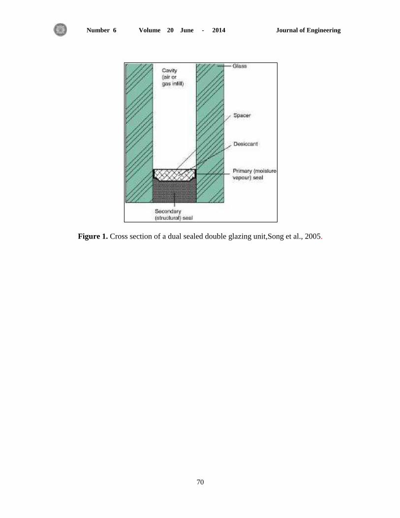
Journal of Engineering Volume 20 June - 2014 Number 6
70
Figure 1. Cross section of a dual sealed double glazing unit,Song et al., 2005.

Journal of Engineering Volume 20 June - 2014 Number 6
71
Figure 2. Drained and ventilated and fully bedded window frames. (a) Timber; (b) PVC; (c)
aluminum; (d) timber fully bedded, Garvin and Wilson, 1998.

Journal of Engineering Volume 20 June - 2014 Number 6
72
Figure 3. Thermal resistances (5cm thickness) of common building insulation materials
(Concrete block is added for comparison purposes), Al-Homoud, 2004.

Journal of Engineering Volume 20 June - 2014 Number 6
73
Figure 4. Air Conditioning plans layout.

Journal of Engineering Volume 20 June - 2014 Number 6
74
.Figure 5. HAP space properties.
Table 1. Monthly simulation results for non-insulated house package unit.

Journal of Engineering Volume 20 June - 2014 Number 6
75
Figure 6. Insulated roofs, walls, floors, and double glazing windows (Researcher).
Table 2. U-Values.
Portion U-Value Non-insulated
Btu/ F ft2 h
U-Value insulated
Btu/ F ft2 h
roofs 0.345 0.06
walls 0.301 0.085
windows 1.228 0.717

Journal of Engineering Volume 20 June - 2014 Number 6
76
Figure 7. HAP U-Value and R-Values for Non-Insulated wall (Researcher).
Table 3. Monthly simulation results for insulated house package unit.

Journal of Engineering Volume 20 June - 2014 Number 6
78
Studying the Effects of Contamination on Soil Properties Using
Remote Sensing
Dr. Mahdi O. Karkush
Instructor
College of Engineering-University of Baghdad
Dr.Abdul Razak T .Ziboon
Professor
University of Technology
[email protected] Hadeel M. Hussien
Researcher
College of Engineering-University of Baghdad
ABSTRACT
The problem of soil contamination is increased recently due to increasing the industrial
wastes such as petroleum hydrocarbon, organic solvents, and heavy metals as well as
maximizing the use of agricultural fertilizers. During this period, wide development of data
collection methods, using remote sensing techniques in the field of soil and environment
applications appear and state the suitable technique for remediation. This study deals with the
application of remote sensing techniques in geoenvironmental engineering through a field
spectral reflectance measurements at nine spots of naturally hydrocarbons contaminated soil
in Al-Daura Refinery Company site which is located to the south west of Baghdad using
radiometer device to get standard curves of wavelengths and analyzing the satellite imagery
of the site to get the spectral reflectance curves using GIS technique and EARDAS software
package which help in producing thematic maps for the spatial distribution and concentration
of contaminants. The comparison of results showed a good correlation between the spectral
reflectance from field measurements and the spectral reflectance obtained from analyzing the
satellite imagery. The study also improves a method to save cost, time, efforts and staff.
Key Words: contaminated soil, remote sensing, spectral reflectance and geoenvironmental
engineering.
بعذعن دراسة تأثر التلىث على خىاص التربة بأستخذام طرق التحسس النائ واالستشعار
د.مهذي عبذ كركىش
مذرس
كلة الهنذسة/جامعة بغذاد
د.عبذالرزاق طارش زبىن
استار
الجامعة التكنىلىجة
هذل ماجذ حسن
هباحث
كلة الهنذسة/جامعة بغذاد
الخالصة
ببنىقج انحبضش خجت نضبدة انخهفبث انصبعت ببىاعهب, انفطت, انزببث انعضىت, ا يشكهت انخهىد اصدادث
انعبد انثقهت وكزنك االفشاط ف اعخخذاو االعذة انضساعت. وبعذ انخطىس انىاعع, ظهش االعخبد عهى طشق
بك انخشبت وانبئت نخحذذ جع انبببث االسضت وانخطبقبث انبئت نالعخشعبس ع بعذ ف حقىل هذعت يك
يقذاس انضشس انبحج ي وجىد هز انهىثبث عهى انخشبت وححذذ طشق انعبنجت انبعبت. هز انذساعت حخعبيم
حغخخذو حقبث انخحغظ انبئ واالعخشعبس ع بعذ ف هذعت انخشبت انهىثت ورنك ي خالل قبط االعكبعت
انخشبت انهىثت طبعب ببنهذسوكبسبىبث وانشصبص ف يصفى انذوسة انىاقع انى انطفت يىقعب نخغعت قبط ي
انجىة انغشب ي بغذاد ببعخخذاو جهبص انشادىيخش وححهم انصىسة انفضبئت نهىقع نغشض انحصىل عهى
. سبطج EARDASيحبث االعكبعت انطفت ببعخخذاو حقبث ظى انعهىيبث انجغشافت واعخخذاو بشبيج
01انخبئج انخ حى انحصىل عههب ي انشادىيخش يع انخبئج انخ حى انحصىل عههب ي انحقبت انبشايجت
EARDAS وبج انخبئج وجىد سبظ جذ ب يحبث قبط االعكبعت انطفت ببنىقع وانصىسة انفضبئت ,
عت يشبكم حهىد انخشبت.وانزي بذوس ىفش ف انجهذ وانكهفت وانىقج انالصو نذسا

Journal of Engineering Volume 20 June - 2014 Number 6
79
1. INTRODUCTION
The rapid growth of industrialization and urbanization has resulted in large quantities
of waste gas, waste water, and waste solid being discharged into the environment,
thus giving rise to serious environmental pollution problem. The occurrences of
contaminants in soil above a certain level causing deterioration or loss some of
geotechnical properties of soil , Huang, 2000. The most common soil contaminants
are petroleum hydrocarbons, fertilizers and pesticides, and heavy metals. Iraq has
several thousand contaminated sites resulting from a combination of general industrial
activities, military activities and post-conflict damage and looting, UNEP Report,
2005.
The great demand for information about properties of surface and sub-surface soil
which can be estimated by using spectral responses of surface soil for different bands
of radiometer and short time available for the work arises to employ remote sensing
techniques in geotechnical engineering which reduce the time, cost, efforts, and staff.
Yousif, 2004, used the remote sensing techniques to classify the soil of Al-Najaf city
by comparing the results obtained from remote sensing techniques with those
obtained from traditional classification method. Al-Maliky, 2005. constructed maps
explained the zones of distributions and concentrations of pollutants in air, water and
soil depending on an integrated measured and collected data base utilizing from GIS
and Arcview software. Carr et al. 2006, used PXRF metal analyzer to obtain rabid
in-situ elemental analysis for urban soil to produce a spatial maps for the distribution
of contaminants in soil. Nasir , 2008, used the surface geoelectrical sounding data and
remote sensing techniques in the evaluation of geotechnical properties of soil, the
results of this study were five contour maps and digital geotechnical maps, as well as
five geoelectrical sections to study the soil profile. Wu et al., 2009, studied the
sensitivity of near-infrared diffuse reflectance sensing (NIRS) to trace metal
concentration in (25) soil samples of silt loam soil. Detailed analysis indicates that the
NIR spectrum is sensitive to sample handling, including the orientation of the samples
in the NIRS instrument.
The purpose of the present work is to measure the reflectance ratio for nine naturally
contaminated soil samples designated N1 to N9 by using three bands radiometer and
compare with those data obtained from satellite image analysis using Arch GIS and
ERDAS10 software.
2. EXPERIMENTAL WORK
2.1. Study Area
The study area is Al-Daura refinery company site which is located at Al-Daura district
in the south-west of Baghdad governorate. Nine spots are selected in this site
according to the advice of environmental staff in the Midland Refineries
Company/Daura Refinery Company as well as the natural ground surface color. The
soil profile of site is formed of top layer of very stiff to hard cohesive material about
(8m) thick, overlying cohesion less layer of dense silty sand (6 to 8) m thick. The
third layer at a depth of 16 m from ground surface consists of hard brown clayey silt.
Groundwater table varied from (1.45 to 2.85) m below the ground surface (NCCL
Report) as cited by , Abdul Rasool , 1999. Disturbed soil samples were obtained from
ground surface to a depth of 15cm for chemical test and particle size analysis.

Journal of Engineering Volume 20 June - 2014 Number 6
80
2.2. GPS Measurements
Soil samples location from the study area are determined by using global positioning
system (GPS) receiver. The spatial position of target can be determined by the GPS
receiver for soil samples location which are located on topographic map using the
Universal Transverse Mercator (UTM) system which is a global spatial system based
on the transverse Mercator projection , Clarke, 1997. The coordinates of position are
referred to as Easting and Northing, being distances East and North of an origin. They
usually expressed in meters. Under the UTM system, each East and North coordinate
pair can refer to one of sixty points on Earth, one point in each of the sixty zones
(World Geodetic System, WGS 84). The geo-referencing data of these locations are
listed in Table 1. and the locations of these points are specified on the satellite
imagery as shown in Plate 1.
2.3. Chemical Tests
The hydrocarbons and lead content of soil samples are determined in Ibn Sina State
Company to measure the effects of hydrocarbons and lead on the reflectance ratio.
The results of tests are given in Table 2.
2.4. Particle Size Analysis
The soil samples are collected from the surface layer of Al-Daura site to determine the
particle-size distribution according to ASTM (D422). The results of particle size
distributions are given in Table 3.
3. SPECTRAL REFLECTANCE MEASUREMENT
3.1 Radiometer
Radiometer is a device used for measuring the spectral reflectance of an object as a
function of wavelength. It is used to measure the reflectance for different targets,
which is reflected, scattered, transmitted, or emitted by an object , Joseph and
Simonett, 1976. Any earth target receives solar radiation directly (irradiance E) by
unit (Watt/m2), otherwise, reflectance radiation from the same target (radiance L),
with same unit radiometer records. This radiation as electrical signal must be
transferred to radiation (Watt/m2) by using the following equation:
L=C1V1 (1)
where
C1: constant transfer factor for each spectral band, each constant has two values: the
first is used for radiance radiation and the second is used for the irradiance radiation.
V1: electromagnetic radiation that is recorded by radiometer, similarly, the irradiance
radiation (E) is given by:
E= C2V2 (2)
In the present study, the radiometer (EXOTH, 1000BX) with three filters of spectral
reflectance bands ranged from (0.45 to 0.7) micrometer as given in Table 4 has been
used to measure the intensity of the reflected waves that come from the soil in vertical
direction. The measurements of radiometer are unit less and can be expressed as

Journal of Engineering Volume 20 June - 2014 Number 6
81
percentage between the reflectance of falling waves from the sun and their reflected
intensity from the soil , Manual of Radiometer, 1983.
The spectral reflectance of soils can be useful in their identification and
characterization. The reflectance data from carefully selected wavelength bands
radiometer can be used to extract information from bare soil areas that can be related
to levels of organic matter, soil moisture, iron oxide content, particle size content, or
used as an indicator of potential productivity such as: cation exchangeable capacity
(CEC) for certain specified climatic areas. The soil contrast is often found in the
wavelength interval from 0.6 to 0.7 µm , Colwell, 1983.
3.2 Conditions of Test
To use the radiometer device in measuring the reflectance ratio of surface soil, the
following conditions must be satisfied:-
i. The target sample should be well represented to region in order to get more
occurrences in measurement;
ii. Readings should be taken for several points closed from the target in the same soil
specimen and calculate their average for more occurrences;
iii. The radiometer should be fixed on the target in order to get constant distance
between the radiometer and soil sample surface. That is required to ensure no
movement of the radiometer during reflectance testing;
iv. All readings are carried out in a sunny weather.
The spectral reflectance measurements of soil samples are carried out at the day time
between 10 and 12 am in order to minimize the effect of the angle of in chiding from
the sun.
3.3 Procedures of Test
The procedure of spectral reflectance test can be summarized as follows:-
i. The test is conducted on the surface of natural soil at the field;
ii. The radiometer is applied to the sunlight direction and recorded the reading;
iii. The radiometer is applied vertically above the target by a vertical distance of
15cm;
iv. The reflectance is read and recorded.
3.4 Spectral Reflectance Analysis
The properties of soils that govern their spectral reflectance are color, texture,
structure and surface roughness, particle size, mineralogy, organic matter, free
carbonates, salinity, moisture and the oxides/hydroxides of iron and manganese,
emissivity, polarizing properties and soil normalization. Also, the chemical
composition of the soil influences spectral signature of soils through the absorption
processes , Manchanda et al., 2002.
Radiometer capacity to measure the visible adds a valuable dimension to the use of
soil spectra to explain many soil characteristics and to predict soil response to
different contaminations, management, and variations in climate , Colwell, 1983.
Soils can often be distinguished by their photographic tone and/or color
characteristics factors which depend on the properties of soil materials themselves.

Journal of Engineering Volume 20 June - 2014 Number 6
82
Also, electromagnetic, radiation can be sensed by detectors that respond in spectral
regions beyond those discernible by human eye , Colwell, 1983. In order to use
remote sensing techniques to produce thematic map explain the zoning of soil
contaminants distribution, it's necessary to understand the relationship between soil
properties and soil color. The most important factors influencing soil color are
mineralogy, chemical composition, moisture content and organic matter content.
4. SATELLITE IMAGE PROCESSING AND ANALYZING
The processing and analysis of satellite imagery can be summarized by the following
procedure:
i. Geo-referencing Spatial Data
Geo-referencing is the conversion of spatial information from an existing format
(collected data and tested samples) in to a digital format and data structure compatible
with a GIS. Geo-referenced data to be encoded include hard copy paper maps and
tables of attributes electron files of maps and associated attribute data, scanned aerial
photographs and digital satellite remotely sensed data (form GPS device). The
traditional digitizing of points is based on the use of Cartesian coordinates such as
UTM coordinates , Jensen, 1996.
ii. Analyzing Spatial Data
The satellite image for AL-Daura site is analyzed by using software (EARDAS 10) to
get the reflectance of geo-referenced data (soil samples locations) depending on the
results of radiometer measurements for soil samples in the field. Data not in image
form are difficult to reduce or associate with specific ground elements unless
simultaneous bore-sighted photography is available.
iii. Classification Process
Multispectral classification is the process of sorting pixels into a finite number of
individual classes, or categories of data, based on their data file values. If a pixel
satisfies a certain set of criteria, the pixel will be assigned to the class that corresponds
to that criterion. This process is also referred to as image segmentation. Depending on
the type of information, extracted from the original data, classes can be associated
with known features on the ground or can simply represent areas that look different to
the computer.
The classification process breaks down into two parts: supervised and unsupervised.
In supervised classification the analyst designates a set of ?training areas? in the
image, each of which is a known surface material that represents a desired spectral
class. The classification algorithm computes, the average spectral pattern for each
training class, and then assigns the remaining image cells to the most similar class. In
unsupervised classification the algorithm derives its own set of spectral classes from
an arbitrary sample of the image cells before making the class assignments , ERDAS
Field Guide?, 2008.
iv. Organization Spatial Data
The organization of spatial data component includes those functions needs to store
and retrieve data from the data base. The methods used to implement these functions
determine how efficiently the system performs all operations on the data; each
variable is archived in a computer-compatible digital format as a geographically
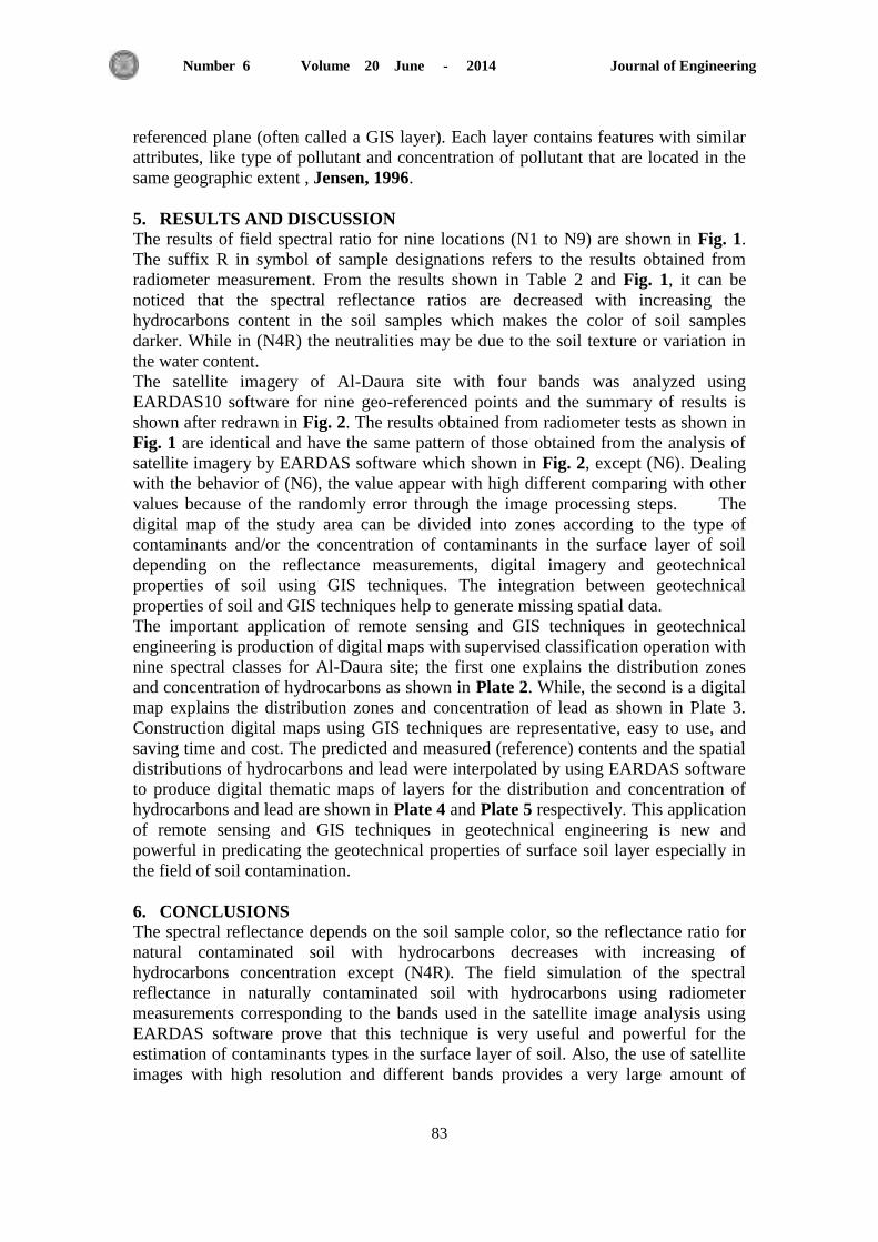
Journal of Engineering Volume 20 June - 2014 Number 6
83
referenced plane (often called a GIS layer). Each layer contains features with similar
attributes, like type of pollutant and concentration of pollutant that are located in the
same geographic extent , Jensen, 1996.
5. RESULTS AND DISCUSSION
The results of field spectral ratio for nine locations (N1 to N9) are shown in Fig. 1.
The suffix R in symbol of sample designations refers to the results obtained from
radiometer measurement. From the results shown in Table 2 and Fig. 1, it can be
noticed that the spectral reflectance ratios are decreased with increasing the
hydrocarbons content in the soil samples which makes the color of soil samples
darker. While in (N4R) the neutralities may be due to the soil texture or variation in
the water content.
The satellite imagery of Al-Daura site with four bands was analyzed using
EARDAS10 software for nine geo-referenced points and the summary of results is
shown after redrawn in Fig. 2. The results obtained from radiometer tests as shown in
Fig. 1 are identical and have the same pattern of those obtained from the analysis of
satellite imagery by EARDAS software which shown in Fig. 2, except (N6). Dealing
with the behavior of (N6), the value appear with high different comparing with other
values because of the randomly error through the image processing steps. The
digital map of the study area can be divided into zones according to the type of
contaminants and/or the concentration of contaminants in the surface layer of soil
depending on the reflectance measurements, digital imagery and geotechnical
properties of soil using GIS techniques. The integration between geotechnical
properties of soil and GIS techniques help to generate missing spatial data.
The important application of remote sensing and GIS techniques in geotechnical
engineering is production of digital maps with supervised classification operation with
nine spectral classes for Al-Daura site; the first one explains the distribution zones
and concentration of hydrocarbons as shown in Plate 2. While, the second is a digital
map explains the distribution zones and concentration of lead as shown in Plate 3.
Construction digital maps using GIS techniques are representative, easy to use, and
saving time and cost. The predicted and measured (reference) contents and the spatial
distributions of hydrocarbons and lead were interpolated by using EARDAS software
to produce digital thematic maps of layers for the distribution and concentration of
hydrocarbons and lead are shown in Plate 4 and Plate 5 respectively. This application
of remote sensing and GIS techniques in geotechnical engineering is new and
powerful in predicating the geotechnical properties of surface soil layer especially in
the field of soil contamination.
6. CONCLUSIONS
The spectral reflectance depends on the soil sample color, so the reflectance ratio for
natural contaminated soil with hydrocarbons decreases with increasing of
hydrocarbons concentration except (N4R). The field simulation of the spectral
reflectance in naturally contaminated soil with hydrocarbons using radiometer
measurements corresponding to the bands used in the satellite image analysis using
EARDAS software prove that this technique is very useful and powerful for the
estimation of contaminants types in the surface layer of soil. Also, the use of satellite
images with high resolution and different bands provides a very large amount of

Journal of Engineering Volume 20 June - 2014 Number 6
84
qualitative and quantitative information for study area to state the soil contamination
states.
REFERENCES
Abdul Rasool H., 1999, Some Geotechnical Properties of Oil Contaminated Soil,
M.Sc. Thesis, University of Baghdad.
Al-Maliky, M. A. S., 2005, Evaluation of Air, Water and Soil Pollutants in Baghdad
City Using Geographic Information System (GIS), M.Sc. Thesis, College of Sciences,
University of Baghdad. (in Arabic).
Annual Book of ASTM Standards, 2003, Soil and Rock; Building, Stone; Peats.
Carr R., Zhang C., Moles N., and Harder M., 2007, Identification and Mapping of
Heavy Metal Pollution in Soils of a Sports Ground in Galway City, Ireland, Using a
Portable XRF Analyser and GIS, Environ Geochem Health, Vol.30, PP. 45? 52.
Clarke K.C., 1997, Getting Started with Geographic Information Systems, University
of California, Santa Barbara. Prentice Hall, Upper Saddle River, New Jersey.
Colwell R.N., 1983, Manual of Remote Sensing, American Society of
Photogrammetry, Volume II.
ERDAS Field Guide?, 2008, Volume I, II.
Huang P. M., 2000, Soils and Ground Water Pollution and Remediation. Asia, Africa,
and Oceania, Lewis Publishers.
Jensen J. R., 1996, Introductory Digital Image Processing a Remote Sensing
Perspective, Second Edition. Prentice Hall. Upper Saddle River, New Jersey.
Joseph L. J. and Simonett D. S., 1976, Remote Sensing of Environment, Addison-
Wesley Publishing Company.
Manchanda, M. L., Kudrat, K. & Tiwari, A. K., 2002, Soil Survey and Mapping Using
Remote Sensing, Regional Remote Sensing Service Centre, Dehradun 248001, India.
Manual of Radiometer, 1983, Exoth Company, U. S. A.
Nasir, A. N. I., 2008, Geotechnical Engineering Study for Salah Al-Din Governorate
Using Geophysical and Remote Sensing Techniques, Ph.D. Thesis, Building and
Construction Engineering Department, University of Technology;
UNEP Report, 2005, Assessment of Environmental ?Hot Spots? in Iraq , Report ISBN
92-807-2650-1, France.
Wu C. Y., Jacobson A. R., Laba M., Kim B., and Baveye P. C., 2009, Surrogate
Correlations and Near-Infrared Diffuse Reflectance Sensing of Trace Metal Content
in Soils, Water Air Soil PoVol.209, PP. 377-390.
Yousif, B. F., 2004, The Use of Remote Sensing Techniques in the Classification of
Al-Najaf Soil, M.Sc. Thesis, Building and Construction Engineering Department,
University of Technology.
NOMENCLATURE
C1 and C2: constant transfer factors for each spectral band.
E: the irradiance radiation (Watt/m2).

Journal of Engineering Volume 20 June - 2014 Number 6
85
L: reflectance radiation from the target (Watt/m2).
V1 and V2: electromagnetic radiation that is recorded by radiometer.
Table 1. GPS coordinates of soil samples locations.
Sample
No.
GPS Coordinates
Northing Easting
N1 0447612 3681802
N2 0447607 3681742
N3 0447247 3681867
N4 0447277 3681886
N5 0446932 3682403
N6 0446836 3682350
N7 0446832 3682340
N8 0446761 3681643
N9 0446757 3681650
Table 2. Hydrocarbons and lead contents and particle-size distribution of
soil.samples.
Soil
Sample
Hydrocarbons Content
%
Lead Content
%
Silt
%
Clay
%
N1 0 0.0025 100 -
N2 0.185 0.0022 40 60
N3 0.285 0.0048 50 50
N4 0.644 0.0034 60 40
N5 22.44 0.0233 100 -
N6 3.629 0.0035 15 85
N7 3.225 0.0027 40 60
N8 0 0.0043 50 50
N9 0 0.0035 30 70
Table 3. Particle-size distribution of soil samples.
Soil
Sample
Silt
%
Clay
%
N1 100 -
N2 40 60
N3 50 50
N4 60 40
N5 100 -
N6 15 85
N7 40 60
N8 50 50
N9 30 70
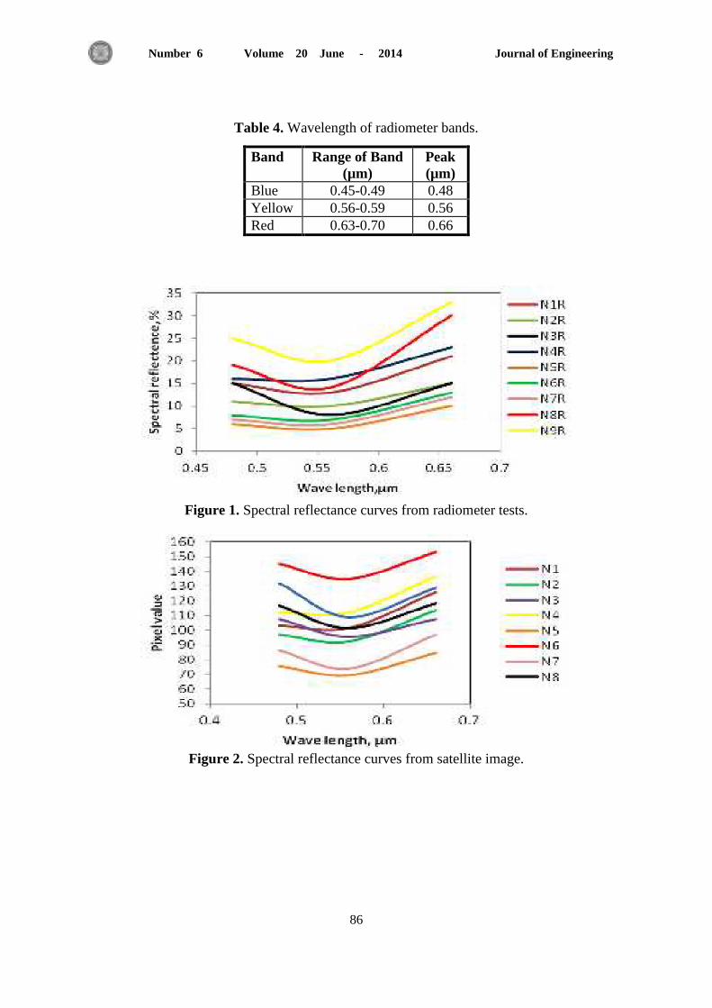
Journal of Engineering Volume 20 June - 2014 Number 6
86
Table 4. Wavelength of radiometer bands.
Band Range of Band
(µm)
Peak
(µm)
Blue 0.45-0.49 0.48
Yellow 0.56-0.59 0.56
Red 0.63-0.70 0.66
Figure 1. Spectral reflectance curves from radiometer tests.
Figure 2. Spectral reflectance curves from satellite image.

Journal of Engineering Volume 20 June - 2014 Number 6
87
Plate 1. Locations of nine spots on satellite image.
Plate 2. Distribution and concentration of hydrocarbons.

Journal of Engineering Volume 20 June - 2014 Number 6
88
Plate 3. Distribution and concentration of lead.

Journal of Engineering Volume 20 June - 2014 Number 6
89
Plate 4. Distribution and concentration of hydrocarbons content in the soil.

Journal of Engineering Volume 20 June - 2014 Number 6
90
Plate 5. Distribution and concentration of lead content in the soil.

Journal of Engineering Volume 20 June - 2014 Number 6
99
The Effect of Ceramic Coating on Performance and Emission of Diesel Engine
Operated on Diesel Fuel and Biodiesel Blends
Ali Abu Al-heel Qasim
Email:
Dr. Mahmoud A. Mashkour
Assistant Professor
Mechanical Engineering
Department-University of
Technology
Email: mahmoud_
Dr. Ibtihal Al-Namie
Assistant Professor
Mechanical Engineering
Department-University of
Technology
Email: [email protected]
ABSTRACT
In this work, the effect of ceramic coating on performance, exhaust gas temperature and
gases emissions of diesel engine operated on diesel fuel and biodiesel blends was investigated. A
conventional four stroke, direct injected, single cylinder, diesel engine was tested at constant speed
and at different load conditions using diesel fuel and biodiesel blends. The inlet and exhaust valves,
the head of piston and cylinder head of the engine were coated by ceramic materials. Ceramic layers
were made of (210-240) μm of Al2O3 and (30-60) μm of 4NiCr5Al as a bond coat for inlet and
exhaust valves and (350-400) μm of YSZ and (50-100) μm of 4NiCr5Al as a bond coat for head of
piston and (280-320) μm of Sic and (40-80) μm of 4NiCr5Al as a bond coat for cylinder head. The
coating technique adapted in this work is the flame spray method. The engine with valves, piston
and cylinder head ceramic coated research was tested for the same operation conditions of the
engine (without coating). The results showed that a reduction in brake specific fuel consumption of
19.29%, 15.91%, 14.65% and 7.06%, an increase in brake thermal efficiency of 23.68%, 19.77%,
16.51% and 6.32%, the increase in exhaust gas temperature of 9.01%, 7.22%, 15.7% and 11.42%,
the reduction of CO emission of 18.57%, 20%, 20.5% and 27.77%, the reduction of HC emission of
28.97%, 43.9%, 38.88% and 36.41% for diesel, B5,B10 and B100 respectively.
Key words: ceramic coating, diesel engine, engine performance, emission, biodiesel.
أنبعاث محرك دسل عمم بىقىد انذسل وخهط ووقىد انذسل انحىيتأحر انطالء انخسف عهى أداء و
د.أبتهال عبذ انرزاق محمىد
أسخار ساعذ
اىجاعت -نائ واىعذاثقس هذست اى
تاىخنىىىج
د.محمىد عطا هللا مشكىر
أسخار ساعذ
اىجاعت -نائ واىعذاثقس هذست اى
تاىخنىىىج
انباحج عه ابى انهم قاسم
انخالصة
ف هزا اىبحذ، ح داسست حأرش اىطالء اىخضف عيى أداء ودسجت حشاسة غاص اىعاد وأبعاد اىغاصاث ىحشك دضه سباع
االشىاط وحق باشش وأحادي االسطىات. ح دساست االداء ىهزا اىحشك بسشعت رابخت وحو خغش باسخخذا وقىد اىذضه اىحىي.
( 042-092 ووجه اىبسخ ووجه االسطىات بىاد خضفت. حذ ح اسخخذا طبقت نىت )ح طالء وجه صا اىذخىه واىعاد
االىىى مسحىق طالء سابط ىطالء صا اىذخىه -مشو-( نشو نو62-02نشو األىىا مادة طالء و )
( نشو 922-52زبخت باىاحشا مادة طالء و )( نشو اىضسمىا اى422-052واىعاد وح اسخخذا طبقت نىت )
( نشو سينى 002-082االىىى مسحىق طالء سابط ىطالء وجه ىبسخ وح اسخخذا طبقت نىت )-مشو–نو
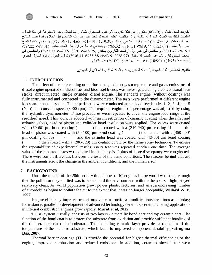
Journal of Engineering Volume 20 June - 2014 Number 6
90
هزا اىعو، االىىى مسحىق طالء سابط ىطالء وجه االسطىات. ف -مشو-( نشو نو82-42اىناسبذ مادة طالء و )
اعخذث حنيىجا اىطالء اىحشاست بخقت اىشش باىيهب. اخخبش اىحشك ححج فس ظشوف اىخشغو قبو اىطالء وقذ اعطج اىخائج
وصادة ف مفاءة اىنبح (%7.26 %،94.65 %،95.99 %،99.09)اىعيت اخفاض ف عذه اسخهالك اىىقىد اىنبح بقذاس
%،7.00 %،9.29) وصادة ف دسجت حشاسة غاص اىعاد بقذاس( %6.00 %،96.59 %،99.77 %،00.68) اىحشاست بقذاس
واخفاض ف (%07.77 %،02.5 %،02 %،98.75) واخفاض ف غاص اوه اومسذ اىناسبى بقذاس (99.40% %،95.7
اىذضه ووقىد اىذضه اىحىي ىىقىد (%06.49 %،08.88 %،40.9 %،08.97) ابعاد اىهذسوماسبىاث غش اىحخشقت بقذاس
%( عيى اىخىاى.922ووقىد اىذضه اىحىي ) (92:92) و (5:95) بسبت خيط
طالء اىسشال، امت اىذضه، اداء اىامت، االبعاد، اىذضه اىحىي.مفاتح انكهمات:
1. INTRODUCTION
The effect of ceramic coating on performance, exhaust gas temperature and gases emissions of
diesel engine operated on diesel fuel and biodiesel blends was investigated using a conventional four
stroke, direct injected, single cylinder, diesel engine. The standard engine (without coating) was
fully instrumented and connected to the dynamometer. The tests were performed at different engine
loads and constant speed. The experiments were conducted at six load levels, viz. 1, 2, 3, 4 and 5
(N.m) and constant speed (3000 rpm). The required engine load percentage was adjusted by using
the hydraulic dynamometer. These procedures were repeated to cover the engine load range at the
specified speed. This work is adopted with an investigation of ceramic coating when the inlet and
exhaust valves, head of piston and cylinder head insulation were applied. The valves were coated
with (30-60) μm bond coating ( ) then coated with a (210-240) μm coating of the
head of piston was coated with (50-100) μm bond coating ( ) then coated with a (350-400)
μm coating of 8% - and the cylinder head was coated with (40-80) μm bond coating
( ) then coated with a (280-320) μm coating of Sic by the flame spray technique. To ensure
the repeatability of experimental results, every test was repeated another one time. The average
value of the repeated testes was adopted in the analysis. Points of large discrepancy were neglected.
There were some differences between the tests of the same conditions. The reasons behind that are
the instruments error, the change in the ambient conditions, and the human error.
2. BACKGROUND
Until the middle of the 20th century the number of IC engines in the world was small enough
that the pollution they emitted was tolerable, and the environment, with the help of sunlight, stayed
relatively clean. As world population grew, power plants, factories, and an ever-increasing number
of automobiles began to pollute the air to the extent that it was no longer acceptable, Willard W. P,
1997.
Engine efficiency improvement efforts via constructional modifications are increased today;
for instance, parallel to development of advanced technology ceramics, ceramic coating applications
in internal combustion engines grow rapidly, Murat et al, 2012.
A TBC system, usually, consists of two layers - a metallic bond coat and top ceramic coat. The
function of the bond coat is to protect the substrate from oxidation and provide sufficient bonding of
the top ceramic coat to the substrate. The insulating ceramic layer provides a reduction of the
temperature of the metallic substrate, which leads to improved component durability, Satrughna
Das, 2007.
Thermal barrier coatings (TBC) provide the potential for higher thermal efficiencies of the
engine, improved combustion and reduced emissions. In addition, ceramics show better wear

Journal of Engineering Volume 20 June - 2014 Number 6
90
characteristics than conventional materials. Lower heat rejection from the combustion chamber
through thermally insulated components causes an increase in available energy that would increase
the cylinder work and the amount of energy carried by the exhaust gases, which could be also
utilized. Thermal barrier coatings are becoming increasingly important in providing thermal
insulation for LHR engine components, Sivakumar et al, 2012.
Dennis Assanis and Kevin Wiese, 1991 studied the effects of ceramic coatings on diesel
engine performance and exhaust emissions. Tests were carried out over a range of engine speeds at
full load for a standard metal piston and two pistons insulated with 0.5 mm and 1.0 mm thick
ceramic coatings. The 0.5mm ceramic coated piston produced 10% higher thermal efficiency than
the metal piston and exhaust CO levels were between 30% and 60% lower than baseline levels.
Similarly, unburned HC levels were 35% to 40% lower for the insulated pistons.
Holloman L. and Levy A.V., 1992, discussed the use of ceramic coatings on the combustion
zone surfaces of large, natural gas-fueled, internal combustion engines was. The performance was
measured in the field before and after coating. It was determined that the durability, power output,
fuel consumption, exhaust emissions, and other operating characteristics all improved due to
ceramic coating of the flame side surfaces of cylinder heads, power pistons, and valves.
Hejwowski T. and Weronski A., 2002, evaluated the effects of thin thermal barrier coatings
on the performance of a diesel engine. Results obtained from the engine with thermally insulated
pistons were compared with the baseline engine data. The performance of the modified engine-
driven car was found satisfactory. The ceramic coating did not produce observable knock in the
engine, no significant wear of piston skirts or cylinder liners was found.
Shrirao P. N. and Pawar A. N., 2011, studied the effect of mullitecoating (Al2O3= 60%,
SiO2= 40%) on a single cylinder, four stroke, direct injection, diesel engine. Tests were carried out
on standard engine (uncoated) and low heat rejection (LHR) engine with and without turbocharger.
The results showed that there was 2.18% decreasing in specific fuel consumption, 12% increasing
in exhaust gas temperature, 22.05% decreasing in CO emission and 28.20% decreasing in HC
emission of LHR engine with turbocharger compared to standard engine at full load.
The aim of this paper is to study the effect of ceramic coating inlet and exhaust valve, head of
piston and cylinder head of diesel engine on the performance of diesel engine operated on diesel fuel
and biodiesel blends and emissions like (CO, CO2, and HC). The results of the two cases are
compared.
3.EXPERIMENTAL WORK
3.1 Coatings Technique
The coating technique adopted in this work is the flame spray method type (rototec 800) as
shown in Fig.1. This apparatus consists of a chamber containing a flange to hold the specimen and
an Oxy- Acetylene flame. The powder particles flow with the flame and is deposited on the
specimen. The powder was supplied through a special tube in the flame gun.
3.2 Coating Procedure
The following procedure was adopted during coating process:
1. The substrates were cleaned and roughened using emery paper (p220) and grit-blasted using
sand blast system with pressure (4-6) bar by sand blast device.
2. The grit-blasted substrates were cleaned using anhydrous ethanol alcohol and dried at 200 °C by
a furnace for 30 min.

Journal of Engineering Volume 20 June - 2014 Number 6
94
3. The ceramic powder type Al2O3 (400 mesh) and 4NiCr5Al metal powder (bond coat) with
particle sizes ranging from 50 to 90 μm for inlet and exhaust valves coating ‒ Fig. 2, 8%Y2O3-
ZrO2 (325 mesh) and (4NiCr5Al) metal powder (bond coat) with particle sizes ranging from 50
to 90 μm for piston coating ‒ Fig. 3 and Sic (200 mesh) and (4NiCr5Al) metal powder (bond
coat) with particle sizes ranging from 50 to 90 μm for cylinder head coating ‒ Fig. 4, were used.
4. The substrate is fixed on the flange normal to the flame and powder flow.
5. The cooling system (air compressor) is switched on to cool the substrates and protect it from
melting during spraying process.
6. The system is switched on and the flame is ignited. The flame holder is controlled manually.
7. The bond powder required for the first layer is loaded into the holder.
8. The substrate is heated to a suitable temperature around (300 °C) by the flame.
9. The coating process is started by moving a lever on the hopper to allow all the powder to flow
through the holder with the flame. A distance of about (20 cm) between the flame and the
specimen is maintained.
10. Step 8 is repeated until 30-60 μm as a thickness of bond layer is obtained for valves, 50-100 μm
for piston and 40-80 μm for cylinder head.
11. The ceramic powder (required for the top coat) is then loaded and step 7 is repeated until 210-
240 μm thickness for valves is obtained, 350-400 μm for piston and 280-320 μm for cylinder
head.
12. The temperature for bond coat and top coat is controlled by adjusting the distance between the
flame and the specimen and the pressure of Oxy-Acetylene.
13. For adhesion process, the topcoat is preheated to about 1500°C directly after completing the
spray process.
14. The flame is then withdrawn gradually away from the valve to minimize thermal shock.
15. After the thermal coating process is completed, the excess parts of coating material are removed
by grinding process to avoid crankshaft breakdown.
3.3 Evaluation of Coating (Bond Strength and Hardness)
The bond strength of coatings is the most important property which determines the field of use
of coatings especially for thermal barrier coatings. The Adhesion strength value between the
substrate and the coating layers was measured using the apparatus type (Microcomputer Controlled
Electronic Universal Testing Machine (WDW-50E). The strength found equals to (26.8) MPa for
8%YSZ, (31.6) MPa for alumina coating and (39.64) MPa for silicon carbide coating. The Adhesion
strength depends on the type of bonding layer and, spraying distance. The hardness value of
(8%YSZ) coating was measured using a Vickers-hardness and found equal to (710) Hv and (788)
Hv for alumina coating and (855) Hv for silicon carbide coating.
3.4 Test Engine Setup and Procedure
The engine tests were conducted in a single cylinder, direct injection (F 170) type diesel
engine. Table 1 presents the main technical specifications of the engine used and Fig. 5 shows it.
This engine was coupled to a calibrated hydraulic dynamometer for speed and torque measurements.
They were fixed on the stainless steel base type (TD 114) which was designed for this purpose. The
water is used as a friction fluid for dynamometer. The system of fuel measurement consumption
consists of a tank with capacity (4.5 l) and a glass tube of known volume was used. The
measurement of air consumption consists of an air box which is used to reduce the vibration

Journal of Engineering Volume 20 June - 2014 Number 6
95
presented when the engine is working with a water manometer. The schematic diagram of the
experimental set up is shown in Fig. 5. The temperature of exhaust gases was measured by
temperature digital indicator (code 952416) that is fixed at the entrance of exhaust gas pipe (the
beginning of the exhaust gas exit). The exhaust gases analyzer type (FLUX 2000-4) was used to
analyze exhaust gases. The gases are picked up from the engine exhaust pipe by means of the probe.
They are separated from the water they contain through the condensate filter and then they are
conveyed to the measuring cell. A ray of infrared light is sent through the optical filters on to the
measured elements. The gases which contain the measuring cell absorb the ray of light at different
wavelength, according to their concentration. The engine was allowed to run with neat diesel fuel
and biodiesel blends at a constant speed for nearly 10 min to attain the steady-state condition at the
lowest possible load. The performance of engine was observed at a constant speed of 3000 rpm and
varying load. To avoid interface between valves and the piston head due to valves coating, a gasket
with 0.3 mm thickness (thickness of valve coating) was inserted between valves and piston head
which works to withdraw valves from the piston head and thus maintain the overlap time and the
standard piston was machined to remove material equal to the desired coating thickness and to keep
the compression ratio unchanged.
3.5 Fuels Used
In this study the commercial diesel fuel employed in the tests was obtained locally and
alternative used fuel substitute for diesel fuel was biodiesel with the mixing ratio of 5:95, 10:90 of
biodiesel to diesel fuel and 100% biodiesel. The marketing specifications of fuel used as provided
from chemical engineering department in technology of university are shown in table 2. To avoid
isolation when biodiesel mixed with diesel fuel, solenoid driven dosing pump type (AQUA) was
used as a fuels mixer. Where each type of fuel enters the pump through two different tubes and go
out of one tube, thus both types of fuel are mixed well. Laboratory samples of Biodiesel was
prepared by mixing alcohol (methanol) with KOH as a catalyst in a tank and then added sunflower
oil heated to 55°C to the tank and then the resulting solution was mixed well for about 30 minutes
and stored for 24 hour. Then be observed biodiesel layer to the top and glycerol layer to the bottom.
Then biodiesel layer was separated from the lower layer and mixed well with water for 10 minutes
as well as the resulting solution was left for 24 hour. Then the upper biodiesel layer was separated
from water layer and heated to 100°C to eliminate water moisture. The biodiesel production is
shown in Fig. 6.
Mathematical relationships used to calculate engine performance is, Ganesan, 2008, Mohanty,
2007.
1. Fuel consumption:(Kg/s)
(1)
where:
- volume of fuel consumption ( )
2. Brake power :(kW)
(2)
Where:

Journal of Engineering Volume 20 June - 2014 Number 6
96
Tb - torque of engine (N.m)
N- rotational speed (rpm)
3. Brake Specific Fuel Consumption:
(3)
4. Brake thermal efficiency:
(4)
(5)
Where:
L.C.V- lower calorific value of kilogram fuel (kJ/kg)
-combustion efficiency (assuming=97%)
The coating technique in this work is the flame spray method type (rototec 800).this apparatus
consists of a chamber containing a flange to hold the specimen and an Oxy-Acetylene flame. The
powder particles flow with the flame and is deposited on the specimen. The powder was supplied
through a special tube in the flame gun.
4. RESULTS AND DISCUSSION:
4.1 Brake Specific Fuel Consumption:
Figs. 7, 8, 9 and 10 indicate the variations of the BSFC for diesel fuel and biodiesel blends
before and after ceramic coating under various engine torques. The BSFC of LHR engine at all
torques is lower than the standard engine with diesel fuel and biodiesel blends. The main reason is
that the ceramic materials will act as barrier for the heat transfer to the surroundings from the
components engine’s combustion chamber and reduces the heat loss from the engine. Also as per
first law of thermodynamics, the heat reduction in heat loss will ultimately increase the power
output and thermal efficiency of the engine and this lead to reduce the BSFC.
4.2 Brake Thermal Efficiency:
The variation of BTE with engine torque is shown in Figs.11, 12, 13 and 14 for base engine
and TBC engine for different fuels under various engine torques. The TBC engine reports better
performance than the base engine. Improved brake thermal efficiency was observed in TBC engine
at all torques. The thermal barrier coating in combustion chamber improves the BTE when
compared with base engine. Since the thermal barrier coating prevents the heat loss from the walls
to the surroundings. The BTE was increased due to the reduction in heat transfer from the gases to
the walls during the combustion or expansion because of the higher wall temperatures. Thin thermal
barrier coating shifts the combustion from premixed to diffusion stage.
4.3 Exhaust Gas Temperature:
Figs. 15, 16, 17 and 18 show the variations of EGT for base engine and TBC engine for
different fuels. It is concluded that the EGT is higher for the engine with ceramic coated components

Journal of Engineering Volume 20 June - 2014 Number 6
97
than the engine under normal conditions and with different fuels. This is due to the raise in the
temperature of the mixture inside the combustion chamber and decrease in heat losses going into the
cooling system and outside due to the coating and due to increase in amount of fuel burnt per unit
time.
4.4 Emissions:
Figs. 19, 20, 21 and 22 show CO variations for base engine and TBC engine for different fuels
under various engine torques. It is clear that CO is decreased after the coating due to the complete
combustion. CO emission from diesel engine is related to the fuel properties as well as combustion
characteristics. It is well known that better fuel combustion usually resulted in lower CO emission.
The carbon monoxide, which arises mainly due to incomplete combustion, is a measure of
combustion efficiency. Generally, oxygen availability in diesel fuel and biodiesel blends is high so
at high temperatures carbon easily combines with oxygen and reduces the CO emission.
Figs. 23, 24 and 25 show variations of HC emissions with torque of the engine before and
after ceramic coating. In general, it is clear that the unburned hydrocarbon emissions are reduced
when the engine works with coating. HC emission is low in the LHR engine with compared with the
standard engine. The emission of unburned hydrocarbon from the LHR engines is more likely to be
reduced because of the decreased quenching distance and the increased lean flammability limit. The
higher temperatures both in the gases and at the combustion chamber walls of the LHR engine assist
in permitting the oxidation reactions to proceed close to completion.
5. CONCLUSION
In this study, the effect of ceramic coating on the performance, exhaust gas temperature and
gases emissions characteristics of a diesel engine operated on diesel fuel and biodiesel blends were
experimentally investigated. Based on the experimental results of this study, the following
conclusions were drawn.
The BSFC of LHR engine were found to be lowered than BSFC of SE due to the effect of
ceramic insulation which act as a barrier for the heat transfer to the surrounding and reduces
the heat loss from the engine. These reductions were up to 19.29%, 15.91%, 14.65% and
7.06% for diesel fuel, B5, B10 and B100 respectively.
The BTE of LHR engine were found to be higher than BTE of SE due to the reduction in heat
transfer from the gas to the walls during the combustion or expansion because of the higher
wall temperatures. These increasing were up to 23.68%, 19.77%, 16.51% and 6.32% for
diesel fuel, B5, B10 and B100 respectively.
The EGT of LHR engine were found to be higher than EGT of SE due to the raise in
temperature of mixture inside the combustion chamber and decrease in heat losses going into
the cooling system. These increasing were up to 9.01%, 7.22%, 15.7% and 11.42% for diesel
fuel, B5, B10 and B100 respectively.
Particulate emissions decreased clearly in LHR engine compared with SE engine due to the
more complete combustion in the insulated configurations. These reductions were up to
18.57%, 20%, 20.5% and 27.77% for CO of diesel, B5, B10 and B100 respectively and
28.97%, 43.9%, 38.88% and 36.41% for HC of diesel, B5, B10 and B100 respectively.

Journal of Engineering Volume 20 June - 2014 Number 6
98
NOMENCLATURE
CO-carbon monoxide
HC- hydrocarbons (ppm)
CO2-carbon dioxide
B5-5:95 of biodiesel to diesel fuel mixing ratio
B10-10:90 of biodiesel to diesel fuel mixing ratio
B100-100% biodiesel
BSFC-brake specific fuel consumption
YSZ- yttria-stabilized zirconia
LHR- low heat rejection
SE-standard engine
KOH- potassium hydroxide
EGT-exhaust gas temperature
BTE-brake thermal efficiency
Figure 1. The flame spray gun type (rototec 800).
Figure 2. Photographic view of valves (before and after ceramic coating).

Journal of Engineering Volume 20 June - 2014 Number 6
99
Figure 3. Photographic view of piston (before and after ceramic coating).
Figure 4. Photographic view of cylinder head (before and after ceramic coating).
Table1. Main technical specifications of engine.

Journal of Engineering Volume 20 June - 2014 Number 6
922
Figure 5. Diesel engine (the board and engine).
Figure 6. Biodiesel production (Daniel Geller).
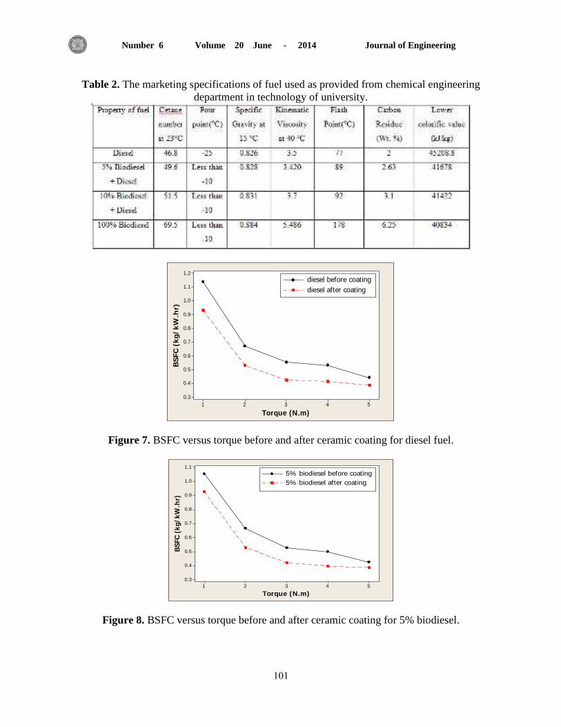
Journal of Engineering Volume 20 June - 2014 Number 6
929
Table 2. The marketing specifications of fuel used as provided from chemical engineering
department in technology of university.
Figure 7. BSFC versus torque before and after ceramic coating for diesel fuel.
Figure 8. BSFC versus torque before and after ceramic coating for 5% biodiesel.
54321
1.2
1.1
1.0
0.9
0.8
0.7
0.6
0.5
0.4
0.3
Torque (N.m)
BS
FC
(k
g/k
W.h
r)
diesel before coating
diesel after coating
54321
1.1
1.0
0.9
0.8
0.7
0.6
0.5
0.4
0.3
Torque (N.m)
BS
FC
(k
g/k
W.h
r)
5% biodiesel before coating
5% biodiesel after coating

Journal of Engineering Volume 20 June - 2014 Number 6
920
Figure 9. BSFC versus torque before and after ceramic coating for 10% biodiesel.
Figure 10. BSFC versus torque before and after ceramic coating for 100% biodiesel.
Figure 11. BTE versus torque before and after ceramic coating for diesel fuel.
54321
1.1
1.0
0.9
0.8
0.7
0.6
0.5
0.4
0.3
Torque (N.m)
BS
FC
(k
g/k
W.h
r)
10% biodiesel before coating
10% biodiesel after coating
54321
1.0
0.9
0.8
0.7
0.6
0.5
0.4
Torque (N.m)
BS
FC
(k
g/k
W.h
r)
100% biodiesel before coating
100% biodiesel after coating
54321
20.0
17.5
15.0
12.5
10.0
7.5
5.0
Torque (N.m)
Bra
ke
th
erm
al e
ffic
ien
cy
diesel before coating
diesel after coating

Journal of Engineering Volume 20 June - 2014 Number 6
920
Figure 12. BTE versus torque before and after ceramic coating for 5% biodiesel.
Figure 13. BTE versus torque before and after ceramic coating for 10 % biodiesel.
Figure 14. BTE versus torque before and after ceramic coating for 100 % biodiesel.
54321
24
22
20
18
16
14
12
10
8
Torque (N.m)
Bra
ke
th
erm
al e
ffic
ien
cy
5% biodiesel before coating
5% biodiesel after coating
54321
24
22
20
18
16
14
12
10
8
Torque (N.m)
Bra
ke
th
erm
al e
ffic
ien
cy
10% biodiesel before coating
10% biodiesel after coating
54321
24
22
20
18
16
14
12
10
Torque (N.m)
Bra
ke
th
erm
al e
ffic
ien
cy
100% biodiesel before coating
100% biodiesel after coating

Journal of Engineering Volume 20 June - 2014 Number 6
924
Figure 15. EGT versus torque before and after ceramic coating for diesel fuel.
Figure 16. EGT versus torque before and after ceramic coating for 5% biodiesel.
Figure 17. EGT versus torque before and after ceramic coating for 10% biodiesel.
54321
400
350
300
250
200
150
Torque (N.m)
Ex
ha
ust
ga
s t
em
pe
ratu
re (
°C
) diesel before coating
diesel after coating
54321
400
350
300
250
200
150
Torque (N.m)
Ex
ha
ust
ga
s t
em
pe
ratu
re (
°C
) 5% biodiesel before coating
5% biodiesel after coating
54321
400
350
300
250
200
150
100
Torque (N.m)
Ex
ha
ust
ga
s t
em
pe
ratu
re (
°C
) 10% biodiesel before coating
10% biodiesel after coating
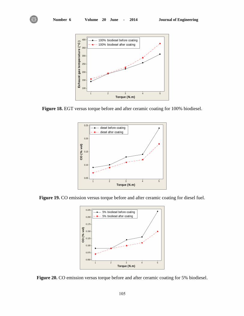
Journal of Engineering Volume 20 June - 2014 Number 6
925
Figure 18. EGT versus torque before and after ceramic coating for 100% biodiesel.
Figure 19. CO emission versus torque before and after ceramic coating for diesel fuel.
Figure 20. CO emission versus torque before and after ceramic coating for 5% biodiesel.
54321
400
350
300
250
200
150
100
Torque (N.m)
Ex
ha
ust
ga
s t
em
pe
ratu
re (
°C
) 100% biodiesel before coating
100% biodiesel after coating
54321
0.25
0.20
0.15
0.10
0.05
Torque (N.m)
CO
(%
vo
l)
diesel before coating
diesel after coating
54321
0.225
0.200
0.175
0.150
0.125
0.100
0.075
0.050
Torque (N.m)
CO
(%
vo
l)
5% biodiesel before coating
5% biodiesel after coating

Journal of Engineering Volume 20 June - 2014 Number 6
926
Figure 21. CO emission versus torque before and after ceramic coating for 10% biodiesel.
Figure 22. CO emission versus torque before and after ceramic coating for 100% biodiesel.
Figure 23. HC emission versus torque before and after ceramic coating for diesel fuel.
54321
0.225
0.200
0.175
0.150
0.125
0.100
0.075
0.050
Torque (N.m)
CO
(%
vo
l)
10% biodiesel before coating
10% biodiesel after coating
54321
0.200
0.175
0.150
0.125
0.100
0.075
0.050
0.025
Torque (N.m)
CO
(%
vo
l)
100% biodiesel before coating
100% biodiesel after coating
54321
250
200
150
100
50
10
Torque (N.m)
HC
(p
pm
)
diesel before coating
diesel after coating

Journal of Engineering Volume 20 June - 2014 Number 6
927
Figure 24. HC emission versus torque before and after ceramic coating for 5% biodiesel.
Figure 25. HC emission versus torque before and after ceramic coating for 10% biodiesel.
6. REFERENCES
Dennis, A. and Kevin, W., 1991, The Effects of Ceramic Coatings on Diesel Engine Performance
and Exhaust Emissions, International Congress and Exposition, Detroit, Michigan, Vol.1.
Daniel, G., UGA Engineering Outreach, http://outreach.engineering.uga.edu/.
Sivakumar, G., et al., 2012, Is Thermal Barrier Coating for Low Heat Rejection in SI Engine or
Diesel Engine, International Journal of Emerging Technology and Advanced Engineering,Vol.2,
Issue12, pp.460-466.
Holloman, L. and Levy, A.V., 1992, Ceramic-Coated Components for the Combustion Zone of
Natural Gas Engines, Journal of Thermal Spray Technology, Vol. 1.
54321
200
150
100
50
10
Torque (N.m)
HC
(p
pm
)
5% biodiesel before coating
5% biodiesel after coating
54321
120
100
80
60
40
20
5
Torque (N.m)
HC
(p
pm
)
10% biodiesel before coating
10% biodiesel after coating

Journal of Engineering Volume 20 June - 2014 Number 6
928
Murat, C., et al., 2012, Ceramic Coating Applications and Research Fields for Internal Combustion
Engines, Ceramic Coatings - Applications in Engineering, Vol.6, pp.978-953.
Shrirao, P. N. and Pawar, A. N., 2011, Evaluation of Performance and Emission Characteristics of
Turbocharged Diesel Engine with Mullite as Thermal Barrier Coating, International Journal of
Engineering and Technology Vol.3, pp.256-262.
Mohanty, R. K., 2007, Internal Combustion Engine, McGraw-Hill book.
Satrughna D., 2007, Study of Plasma Spray Alumina - aluminide Composite Coating on Metals,
National Institute of Technology, Rourkela, India.
Hejwowski T. and Weronski, A., 2012, The Effect of Thermal Barrier Coatings on Diesel Engine
Performance,3rd International Symposium on Applied Plasma Science (ISAPS 01), Vol. 65,
pp.427-432.
Ganesan, V., 2008, Internal Combustion Engine", 3rd Edition, Tata McGraw Hill Book.
Willard, W.P., 2010, Engineering Fundamentals of the Internal Combustion Engin", prentice Hall,
Platteville, 1997. Published by IEEE.

Journal of Engineering Volume 20 June - 2014 Number 6
109
Compression of an ECG Signal Using Mixed Transforms
ABSTRACT
Electrocardiogram (ECG) is an important physiological signal for cardiac disease diagnosis.
With the increasing use of modern electrocardiogram monitoring devices that generate vast amount
of data requiring huge storage capacity. In order to decrease storage costs or make ECG signals
suitable and ready for transmission through common communication channels, the ECG data
volume must be reduced. So an effective data compression method is required. This paper presents
an efficient technique for the compression of ECG signals. In this technique, different transforms
have been used to compress the ECG signals. At first, a 1-D ECG data was segmented and aligned
to a 2-D data array, then 2-D mixed transform was implemented to compress the ECG data in the 2-
D form. The compression algorithms were implemented and tested using multiwavelet, wavelet and
slantlet transforms to form the proposed method based on mixed transforms. Then vector
quantization technique was employed to extract the mixed transform coefficients. Some selected
records from MIT/BIH arrhythmia database were tested contrastively and the performance of the
proposed methods was analyzed and evaluated using MATLAB package. Simulation results showed
that the proposed methods gave a high compression ratio (CR) for the ECG signals comparing with
other available methods. For example, the compression of one record (record 100) yielded CR of
24.4 associated with percent root mean square difference (PRD) of 2.56% was achieved.
Key words: ECG Compression, Wavelet, Multiwavelet and Slantlet Transforms, Vector
Quantization
ضغط اشارة تخطيط القلب باستخذام التحويالت الخليطة
م.م. جليل سعذون جميل .م.د. صادق جاسن ابو اللوخا
قسى انذست انكشبائت قسى انذست انكشبائت
كهت انذست / خايعت بغذاد كهت انذست / خايعت بغذاد
الخالصة
ب. ز االشاسة عادة حشاقب بشكم ( حسخخذو عه طاق اسع ف حشخص عالج ايشاض انقهECGاشاس حخطظ انقهب )
يسخش , زا سؤد ان كاث كبش ي انبااث حخاج حخزا ا قها .نزنك خطهب سه فعان نضغظ ز انبااث .
ف زا انبحث ححالث يخخهفت نضغظ اشاساث حخطظ انقهب حى أسخخذايا . ف انبذات خى ححم اشاساث حخطظ انقهب
اث راث بعذ احذ ان اشاساث راث بعذ , ثى بعذ رنك خى ضغظ عز االشاساث بأسخخذاو خهظ ي انخحالث .طشقت انضغظ اشاس
اعخادا عه خهظ يخخهف حث حى حشكم طشق يخخهفت multiwavelet Wavelet slantetحى حفزا باسخخذاو انخحاث
نخشفش انعايالث اناحدت ي انخحالث انخخهطت . VQو نز انخحاث .ثى بعذ رنك حى اسخخذا
( حى ححهم اداء انطشق انقخشحت Mit-BHI arrhythmia databaseحى أخخاس اشاساث حخطظ انقهب ي قاعذة انبااث )
ت الشاساث حخطظ .بج خائح انحاكاة ا انطشق انقخشحت حعط سب ضغظ عانMATLABحقا ي خالل اسخخذاو بشايح
Sadiq Jassim Abou-Loukh
Assistant Professor
College of Engineering-University of Baghdad
Email: [email protected]
Jaleel Sadoon Jameel
Instructor
College of Engineering-University of Baghdad
Email: [email protected]
Journal of Engineering Volume 20 June - 2014 Number 6
110
( باسخخذاو انطشق record 100انقهب بانقاس يع انطشق االخش انخفشة .عه سبم انثال، ضغظ اشاس حخطظ قهب احذ )
% . 2,,4ي سب خطا حسا 42,2انقخشح اعطج سب ضغظ حسا
1. INTRODUCTION
ECG is widely used in the diagnosis and treatment of cardiac disease. ECG signals usually
continuously monitored and this will lead large amount of data needs to be stored or transmitted.
ECG compression becomes mandatory to efficiently store and retrieve this data from medical
database, Polania, et al., 2011. Compression of ECG is necessary for efficient storage and
transmission of the digitized ECG signals. A typical ECG monitoring device generates a large
amount of data in the continuous long-term (12-24 hours) ambulatory monitoring tasks. For good
diagnostic quality, up to 12 different streams of data may be obtained from various sensors placed
on the patient’s body, Hossain, et al., 2008. Thus, efficient ECG data compression to dramatically
reduce the data storage capacity is a necessary solution. On the other hand, it makes possible to
transmit ECG data over a telephone line from one cardiac doctor to another to get opinions, Wang,
et al., 2008.
Compression methods have gained an importance in recent year in many medical areas like
telemedicine and health monitoring. Many ECG data compression methods have been proposed to
achieve a high compression ratio (CR) result and preserve clinical information. These methods can
be categorized into time-domain, and transform-domain groups. Recently, a wavelet-based approach
attracted much attention of researchers due to both its simplicity and high-compression
performance, Ku, et al., 2010.
There are different ways of merging two or more transforms to form a mixed transforms. The
proposed mixed transforms consists of two transforms in cascading form to be used to enhance
compressing performance. Different schemes of applying wavelet, multiwavelet, and slantlet
transforms are implemented. The results are obtained through simulation by MATLAB package in
this work.
This paper is organized as follows: ECG compression techniques are explained in section II. The
standard quantitative measurements that used for ECG are presented in section III. Section IV
describes the proposed compression algorithms. Simulation results and comparisons with other
compression algorithm in the literature are presented in section V. Finally the conclusion is given in
section VI.
2. ECG COMPRESSION TECHNIQUES
The main goal of any compression technique is to achieve maximum data volume reduction while
preserving the significant features, Khalaj, and Naimi, 2009. A compression algorithm takes an
input X and generates a representation XC that hopefully requires fewer bits. There is a
reconstruction algorithm that operates on the compressed representation XC to generate the
reconstructed presentation Y.
2.1 Discrete Wavelet Transform
Wavelets are mathematical functions that provide the time-frequency representation. It cuts up
data into different frequency components, and then study each component with a resolution matched
to its scale. Most interesting dissimilarities between wavelet and Fourier transforms is that
individual wavelet functions are localized in space, Fourier sine and cosine functions are not,

Journal of Engineering Volume 20 June - 2014 Number 6
111
Graps, 1995. In discrete wavelet transform (DWT) the scale and translate parameters are chosen
such that the resulting wavelet set forms an orthogonal set, i.e. the inner product of the individual
wavelets ψ (j,k) is equal to zero. To this end, dilation factors are chosen to be powers of 2. For
DWT, the set of dilation and translation of the mother wavelet is defined as, Cohen, and Jelena,
1996.
22 2
, ktt jjkj (1)
Where j is the scaling factor and k is the translation factor. It is obvious that the dilation factor is
a power of 2. Forward and inverse transforms are then calculated using the following equations,
Cohen, and Jelena, 1996.
(2)
(3)
For efficient decorrelation of the data, an analysis wavelet set ψ (j,k) should be chosen which
matches the features of the data well. This together with orthogonally of the wavelet set will result
in a series of sparse coefficients in the transform domain, which obviously will reduce the amount
of bits needed to encode it, Zafarifar, 2002. A typical 2-D DWT, used in image compression, it
generates the hierarchical pyramid structure shown in Fig.1.
2.2 Multiwavelet Transform
Multiwavelet has been introduced as a more powerful multi-scale analysis tool. A scalar wavelet
system is based on a single scaling function and mother wavelet. On the other hand, a multiwavelet
uses several scaling functions and mother wavelets, Strela, and Heller, 1999. Multiwavelets,
namely, vector-valued wavelet functions, are a new addition to the classical wavelet theory that has
revealed to be successful in practical applications, such as signal and image compression. In fact,
multiwavelets possess several advantages in comparison to scalar wavelets, since a multiwavelet
system can simultaneously provide perfect reconstruction while preserving orthogonality, symmetry,
a high order of approximation (vanishing moments), etc. Nevertheless, multiwavelets differ from
scalar wavelet systems in requiring two or more input streams to the multiwavelet filter bank,
Liang, et al., 1996.
The multiwavelet idea originates from the generalization of scalar wavelets; instead of one
scaling function and one wavelet, multiple scaling functions and wavelets are used (see Fig. 2). This
leads to more degree of freedom in constructing wavelets. Therefore, opposed to scalar wavelets,
properties such as compact support, orthogonality, symmetry, vanishing moments, short support can
be gathered simultaneously in multiwavelets, which are fundamental in signal process. The increase
in the degree of freedom in multiwavelets is obtained at the expense of replacing scalars with
matrices, scalar functions with vector functions and single mattresses with a block of matrices. Also,
prefiltering is an essential task which should be performed for any use of multiwavelet in the signal

Journal of Engineering Volume 20 June - 2014 Number 6
112
processing, Al-Sammaraie, 2011. Many types of multiwavelet such as Geronimo-Hardin-
Massopust (GHM) and Chui-Lian (CL) multiwavelets have been developed, Xia, et al., 1996.
To implement the multiwavelet transform, a new filter bank structure is required where the
lowpass and highpass filter banks are matrices rather than scalars. That is, the GHM two scaling and
wavelet functions satisfy the following two-scale dilation equations, Liang, et al., 1996.
(4)
(5)
The (2×2) matrix filters in the multiwavelet filter bank require vector inputs. Thus, a 1-D input
signal must be transformed into two 1-D signals.
This transformation is called pre-processing. For some multiwavelet, the pre-processing must be
accompanied by an appropriate pre-filtering operation that depends on the spectral characteristics of
the multiwavelet filters, Xia, 1998.
2.3 Slantlet Transform
Slantlet transform (SLT) has been recently proposed as an improvement over the usual DWT.
The SLT is an equivalent form of the DWT implementation but provides better time-localization
due to the shorter supports of component filters. The SLT filters are essentially piecewise linear
filters, have desirable properties of orthogonality and two vanishing moments, have an octave-band
characteristic, can exactly provide a scale dilation factor of 2, provides a multiresolution
decomposition. The SLT filter-bank is implemented in the form of a parallel structure, employing
different filters for each scale whereas DWT is usually implemented in the form of an iterated filter-
bank, utilizing a tree structure. SLT can exactly provide a scale dilation factor of 2 and is less
frequent selective due to shorter supports of the component filters whereas DWT filters can
approximately provide a scale dilation factor of 2 and provide short windows at high frequencies
and long windows at low frequencies, Kummar, and Muttoo, 2010.
The usual iterated DWT filter-bank and its equivalent form are shown in Fig.3. The slantlet filter-
bank is based on the equivalent structure that is occupied by different filters that are not products.
With this extra degree of freedom obtained by giving up the product form, filters of shorter length
are designed to satisfy orthogonality and zero moment conditions, Selenick, 1999.
For the two-channel case, the shortest filters for filter-bank is orthogonal and has K zero
moments are well known filters described by Daubechies. For K = 2 zeros moments, filters H(z) and
F(z) are of length 4. For this system, the iterated filters in Fig.4 are of length 10 and 4. Without the
constraint that the filters are products, an orthogonal filter-bank with K = 2 zeros moments can be
obtained where the filter lengths are 8 and 4, as shown in Fig.4. That is a reduction by two samples,
which is a difference that grows with the number of stages. This reduction in length, while
maintaining desirable orthogonality and moment properties, is possible because these filters are not
constrained by the product form arising in the case of iterated filter-banks, Selenick, 1999.
kk
kt
ktH
t
t
2
22
2
1
2
1
k
kkt
ktG
t
t
2
22
2
1
2
1

Journal of Engineering Volume 20 June - 2014 Number 6
113
2.4 Vector Quantization
Vector quantization (VQ) is used for both image and sound compression. In practice, VQ is
commonly used to compress data that have been digitized from an analog source, such as sampled
sound and scanned images. Vector quantization is based on two facts, Cosman, et al., 1996.
• The compression methods that compress strings, rather than individual symbols can, in principle,
produce better results.
• Adjacent data items in an image (i.e., pixels) and digitized sound (i.e., samples) are correlated.
There is a good chance that the nearest neighbors of a pixel P will have the same values as P or
very similar values. Also consecutive sound samples rarely differ much.
For signal compression, VQ divides the signal into small blocks of pixels, typically 2×2 or 4×4.
Each block is considered a vector. The encoder maintains a list (called a codebook) of vectors and
compresses each block by writing to the compressed stream a pointer to the block in the codebook.
The decoder has the easy task of reading pointers, following each pointer to a block in the
codebook, and joining the block to the image so far (see Fig.5). Vector quantization is thus an
asymmetric compression method.
An improved algorithm of VQ, codebook generation approaches such as the LBG algorithm has
been developed. LBG algorithm designing a codebook that best represents the set of input vectors is
very-hard. That means that it requires an exhaustive search for the best possible codewords in space,
and the search increases exponentially as the number of codewords increases, therefore, we resort to
suboptimal codebook design schemes, and the first one that comes to mind is the simplest. It is
named LBG algorithm for Linde-Buzo-Gray and also it is known as K-means clustering.
The LGB algorithm is in fact designed to iteratively improve a given initial codebook. The design
of a codebook with N-codewords can be stated as follows, Bardekar, and Tijare, 2011:-
1. Determine the number of codewords, N, or the size of the codebook .
2. Select N codewords at random, and let that be the initial codebook. The initial codewords can be
randomly chosen from the set of input vectors .
3. Use the Euclidean distance to measure cluster size the vectors around each codeword. This is
done by taking each input vector and finding the Euclidean distance between it and each
codeword. The input vector belongs to the cluster of the codeword that yields the minimum
distance .
Compute the new set of codewords. This is done by obtaining the average of each cluster. Add
the component of each vector and divide by the number of vectors in the cluster, Bardekar, and
Tijare, 2011.
(6)
Where i is the component of each vector (x, y, z, directions) and m is the number of vectors in
the cluster.
Repeat steps 1, 2 and 3 until either the codewords do not change or the change in the codewords
is small.
m
jxij
myi
1
1
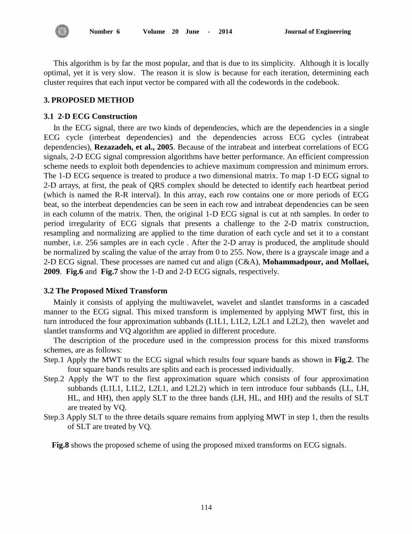
Journal of Engineering Volume 20 June - 2014 Number 6
114
This algorithm is by far the most popular, and that is due to its simplicity. Although it is locally
optimal, yet it is very slow. The reason it is slow is because for each iteration, determining each
cluster requires that each input vector be compared with all the codewords in the codebook.
3. PROPOSED METHOD
3.1 2-D ECG Construction
In the ECG signal, there are two kinds of dependencies, which are the dependencies in a single
ECG cycle (interbeat dependencies) and the dependencies across ECG cycles (intrabeat
dependencies), Rezazadeh, et al., 2005. Because of the intrabeat and interbeat correlations of ECG
signals, 2-D ECG signal compression algorithms have better performance. An efficient compression
scheme needs to exploit both dependencies to achieve maximum compression and minimum errors.
The 1-D ECG sequence is treated to produce a two dimensional matrix. To map 1-D ECG signal to
2-D arrays, at first, the peak of QRS complex should be detected to identify each heartbeat period
(which is named the R-R interval). In this array, each row contains one or more periods of ECG
beat, so the interbeat dependencies can be seen in each row and intrabeat dependencies can be seen
in each column of the matrix. Then, the original 1-D ECG signal is cut at nth samples. In order to
period irregularity of ECG signals that presents a challenge to the 2-D matrix construction,
resampling and normalizing are applied to the time duration of each cycle and set it to a constant
number, i.e. 256 samples are in each cycle . After the 2-D array is produced, the amplitude should
be normalized by scaling the value of the array from 0 to 255. Now, there is a grayscale image and a
2-D ECG signal. These processes are named cut and align (C&A), Mohammadpour, and Mollaei,
2009. Fig.6 and Fig.7 show the 1-D and 2-D ECG signals, respectively.
3.2 The Proposed Mixed Transform
Mainly it consists of applying the multiwavelet, wavelet and slantlet transforms in a cascaded
manner to the ECG signal. This mixed transform is implemented by applying MWT first, this in
turn introduced the four approximation subbands (L1L1, L1L2, L2L1 and L2L2), then wavelet and
slantlet transforms and VQ algorithm are applied in different procedure.
The description of the procedure used in the compression process for this mixed transforms
schemes, are as follows:
Step.1 Apply the MWT to the ECG signal which results four square bands as shown in Fig.2. The
four square bands results are splits and each is processed individually.
Step.2 Apply the WT to the first approximation square which consists of four approximation
subbands (L1L1, L1L2, L2L1, and L2L2) which in tern introduce four subbands (LL, LH,
HL, and HH), then apply SLT to the three bands (LH, HL, and HH) and the results of SLT
are treated by VQ.
Step.3 Apply SLT to the three details square remains from applying MWT in step 1, then the results
of SLT are treated by VQ.
Fig.8 shows the proposed scheme of using the proposed mixed transforms on ECG signals.

Journal of Engineering Volume 20 June - 2014 Number 6
115
4. PERFORMANCE MEASUREMENTS
Evaluation of lossy ECG encoders uses measurements related to the amplitude difference
between the original and the reconstructed signal. The standard quantitative measurement is the
percent root mean square difference (PRD), which is given by the following, Lee, et al., 2012:
100
12))((
12))(~)((
Nn
nx
Nn
nxnxPRD (7)
Where )(nx is the original signal, )(~ nx is the reconstructed signal and n is the number of samples.
Since a lower PRD value indicates that the reconstruction approximates more closely to the
original. However, qualitative evaluations are almost invariably used due to human beings better
judgment of which details of the signal are important
The compression ratio (CR) is a measure of the amount of data size reduction achieved and it is
calculated by, Polania, et al., 2011:
1: size
size
compressed
eduncompressCR (8)
5. RESULTS AND DISCUSSION
The proposed algorithm was tested and evaluated by using an actual data from the MIT-BIH
arrhythmia database, MIT-BIH. This database includes different shapes of ECG signals arranged in
different records. The records used are 100, 107, 109, and 117, which are different in shape of the
ECG signals. Records 100 and 109 have a regular period of QRS compared with the other signals
while records 107 and 117 have an almost regular QRS period.
The results of performing the compression algorithm for the proposed mixed transform using
different types of records are given in the table 1.
This results show that each signal has a different CR than the other signals after applying the
same algorithm. The variation in performance parameters depends on the shape and size of each
ECG signal. For nearly the same values of CR, it is shown that records 100 and 109 have a lower
PRD than records 107 and 117 at the all codebook sizes (256), (64), and (16). This difference in
PRD is due to the regularity of QRS periods in records 100 and 109 compared with records 107 and
117 which have an almost regular QRS period.
The proposed algorithms are also compared to other ECG coders through their reports
performance in the literature. In table 2, PRD and CR comparisons of different coding algorithms
were shown. As the results show, the proposed schemes exhibits better performance than well-
known methods such as those based on matrix completion, Polania, et al., 2011, wavelet transform,
Hossain et al., 2008, and new efficient fractal, Khalaj, and Naimi, 2009.
Figures 9, 10, and 11 show samples of original, reconstructed and error signals for different
types of ECG signals.

Journal of Engineering Volume 20 June - 2014 Number 6
116
6. CONCLUSION
Difference transforms have been used in this paper, using MWT, WT, and SLT which are
employed with the VQ algorithm in different distribution. This distribution was exploited by
cascading manner. The work includes an ECG signal compression method using 2-D mixed
transform. The following points are the summary of the important conclusions:
1. The proposed method offers a compression performance of ECG signal up to 27 with little effects
will be noticed on the ECG quality.
2. The codebook size refers to the total numbers of code vectors in the codebook. As the size of
codebook increase the quality of the reconstructed signal improves, but the compression ratio
reduces. Therefore, there is a tradeoff between the quality of the reconstructed signal and the
amount of compression achieved.
3. The compression performances of the proposed mixed transforms are different from one ECG
signal to another depending on the regularity of the ECG signals. For records that have regular
QRS-complex the PRD will be less than records that has irregular QRS-complex.
7. REFERENCES
- Al-Sammaraie, M. F., 2011, Medical Images Compression Using Modified SPIHT Algorithm and
Multiwavelet Transformation, Computer and Information Science, Vol. 4, No. 6, PP. 2-17.
- Bardekar, A. A., and Tijare, P. A., 2011, Implementation of LBG Algorithm for Image
Compression, International J. of Computer Trends and Technology, Vol. 2, Issue 2, PP. 86-91.
- Cohen, A., and Jelena K., 1996, Wavelets: The Mathematical Background, Proceeding of the
IEEE, Vol. 84, No. 4, PP. 514-522.
- Cosman, P. C., Gray, R. M., and Vetterli, M., 1996, Vector Quantization of Image Sub-bands:
A Survey, IEEE Trans. on Image Processing, Vol. 5, No. 2, PP. 202-225.
- Graps, A., 1995, An Introduction to Wavelets, IEEE Computational Science and Engineering,
Vol. 2, No. 2, PP. 1-18.
- Hossain, M.S., Aziz, T., and Haque, M., 2008, ECG Compression Using Multilevel Thresholding
of Wavelet Coefficients, International Conference on Digital Object Identifier, PP. 321-326.
- Khalaj, A., and Naimi, H. M., 2009, New Efficient Fractal Based Compression Method for
Electrocardiogram Signals, Canadian Conference on Electrical and Computer Engineering
CCECE'09, PP. 983-986.
- Ku, C. T., Hung, K. C., Wu, T. C., and Wang, H., 2010, Wavelet-Based ECG Data Compression
System with Linear Quality Control Scheme, IEEE Trans. on Biomedical Engineering, Vol.57,
No.6, PP. 1399-1409.

Journal of Engineering Volume 20 June - 2014 Number 6
117
- Kumar, S., and Muttoo, S. K., 2010, An Overview of Wavelet-Like Transform and Image Data
Hiding, Proceeding of the 4th National Conference, INDIA.
- Lee, H. W., Hung, K. C., Wu, T. C., and Ku, C. T., 2012, A Modified Run-Length Coding for the
Realization of Wavelet-Based ECG Data Compression System, Journal of Next Generation
Information Technology, Vol. 1, No. 1, PP. 202-210.
- Liang, K.C., Li, J., and Kuo, C. J., 1996, Image Compression with Embedded Multiwavelet
Coding, SPIE Proceeding on Wavelet Applications, Vol. 2762, PP. 165-176.
- Mohammadpour, T. I., and Mollaei, M. R., 2009, ECG Compression With Thresholding of 2-D
Wavelet Transform Coefficients and Run Length Coding, European Journal of Scientific
Research, Vol. 27, No. 2, PP. 248- 257.
- Polania, L. F., Corrillo, R. E., Velasco, M. B., and Barner, K. E., 2011, Matrix Completion Based
ECG Compression, 33rd Annual International Conference of the IEEE EMBS, Boston,
Massachusetts, PP. 1757-1760.
- Rezazadeh, I. M., Moradi, M. H., and Nasrabadi, A. M.,2005, Implementing of SPIHT and Sub-
band Energy Compression Method on 2-D ECG Compression: A Novel Approach, Proceeding of
the IEEE, PP. 1-4.
- Selenick, I. W., 1999, The Slantlet Transform, IEEE Trans. on Signal Processing,Vol.47, No.5,
PP. 1304-1313.
- Strela, V., Heller, P., Strang, G., Topiwala, P., and Heil, C., 1999, The Application of Multiwavelet
Filterbanks to Image Processing, IEEE Trans. on Image processing, Vol. 8, No. 4, PP. 548-563.
- Wang, Z., Zhu, P., and Chen, Y., 2008, A 2-D ECG Compression Algorithm Based on Modified
SPIHT, Proceedings of the 5th International Workshop on Wearable and Implantable Body
Sensor Networks, PP. 305-309.
- Xia, X. G., 1998, A New Prefilter Design for Discrete Multiwavelet Transforms, IEEE Trans. on
Signal Processing, Vol. 46, No. 6, PP. 1558-1570.
- Xia, X. G., Geronimo, J. S., Hardian, D.P., and Suter, B. W., 1996, Design of Prefilter for
Discrete Multiwavelet Transform, IEEE Trans. on Signal Processing , Vol. 44, No. 1, PP. 25-35.
- Zafarifar, B., 2002, Micro-codable Discrete Wavelet Transform, M. Sc. Thesis, Faculty of
Information Technology and Systems, Delft University of Technology, Netherlands.
- MIT-BIH Arrhythmia Database http://www.physionet.org/physiobank/database/mitdb/

Journal of Engineering Volume 20 June - 2014 Number 6
118
Figure1. Pyramid structure of wavelet decomposition.
Figure 2. Resultant multiwavelet transform bands.
Figure 3. Two-scale filter bank and an equivalent structure.

Journal of Engineering Volume 20 June - 2014 Number 6
119
Figure 4. Comparison of two-scale iterated D2 filter bank (left-hand side)
and two-scale slantlet filter bank (right-hand side).
Figure 5. The encoder and decoder in a vector quantization.

Journal of Engineering Volume 20 June - 2014 Number 6
120
Figure 6. Waveform of 1-D ECG signal.
Figure 7. Waveform of 2-D ECG signal.
Am
pli
tud
e
Samples
Samples
Am
pli
tud
e

Journal of Engineering Volume 20 June - 2014 Number 6
121
Figure 8. Proposed scheme of mixed transform and their compression processing.
Figure 9. Original, reconstructed and error for ECG signal of record 100 for CR=24.4 and PRD=2.5%.
2-D
ECG
WT
MWT
SLT
SLT
VQ
Bit stream

Journal of Engineering Volume 20 June - 2014 Number 6
122
Figure 10. Original, reconstructed and error for ECG signal of record 109 for CR=24.3 and PRD=3.1%.
Figure 11. Original, reconstructed and error for ECG signal of record 117 for CR=24.2 and PRD=4.7%.
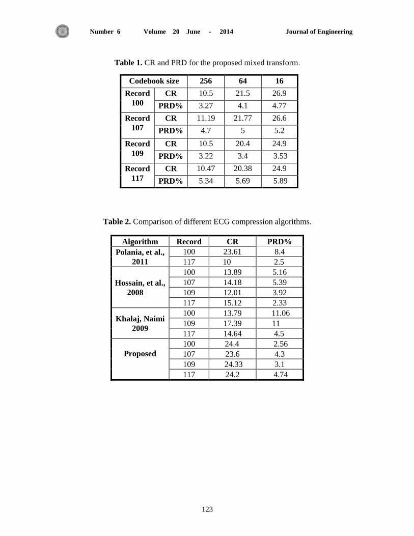
Journal of Engineering Volume 20 June - 2014 Number 6
123
Table 1. CR and PRD for the proposed mixed transform.
Table 2. Comparison of different ECG compression algorithms.
Algorithm Record CR PRD%
Polania, et al.,
2011
100 23.61 8.4
117 10 2.5
Hossain, et al.,
2008
100 13.89 5.16
107 14.18 5.39
109 12.01 3.92
117 15.12 2.33
Khalaj, Naimi
2009
100 13.79 11.06
109 17.39 11
117 14.64 4.5
Proposed
100 24.4 2.56
107 23.6 4.3
109 24.33 3.1
117 24.2 4.74
16 64 256 Codebook size
26.9 21.5 10.5 CR Record
100 4.77 4.1 3.27 PRD%
26.6 21.77 11.19 CR Record
107 5.2 5 4.7 PRD%
24.9 20.4 10.5 CR Record
109 3.53 3.4 3.22 PRD%
24.9 20.38 10.47 CR Record
117 5.89 5.69 5.34 PRD%

Journal of Engineering Volume 20 June - 2014 Number 6
124
Study the Effect of Face Sheets Material on Strength of Sandwich Plates with
Circular Hole
Dr. Hatem Rahem Wasmi
Assistant Professor
College of Engineering-University of Baghdad
Nawal Falkhous Eshaut
Instructtor
College of Engineering -University of Baghdad
ABSTRACT
This study aims to investigate the effect of changing skins material on the strength of
sandwich plates with circular hole when subjected to mechanical loads. Theoretical, numerical and
experimental analyses are done for sandwich plates with hole and with two face sheet materials.
Theoretical analysis is performed by using sandwich plate theory which depends on the first order
shear deformation theory for plates subjected to tension and bending separately. Finite element
method was used to analyse numerically all cases by ANSYS program.
The sandwich plates were investigated experimentally under bending and buckling load
separately. The relationship between stresses and the ratio of hole diameter to plate width (d/b) are
built, by studying the effect of hole size on strength of sandwich plates. The maximum stress were
developed at the hole region in sandwich plates clarified the dropped in their strength. So, the
experimental maximum stress was found by means of multiplying the experimental nominal stress
obtained from Stress-strain curve by the stress concentration factor.
All results which obtained, theoretically, numerically and experimentally are compared to find
that the hole weaken the strength of sandwich plates because of the stress concentration and that
weakness is depending on the hole size and the face sheets materials.
Keywords: sandwich plate, hole size, sandwich plate theory, stress concentration.
الشطيريح, زدم الثقة, وظريح الصفائر الشطيريح, ذمركز اإلخاذاخالصفائر الكلمات الرئيسية:
دراسة تأثير مادة القشرة على مقاومة الصفائح الشطيرية المثقوبة
الخالصة
ألزمددا ا ا الدد ذعرضددالمثقتددح عىددر مقامددح الصددفائر الشددطيريح علدد مدداذج القشددرج ذدديرير تسدد ذددره ددلي الر الددح لدد
عمليدا. ذدم الرسليدل الىظدر وظريدا يال لدذس الصفائر الشطيريح المثقتح تالرعما وعيه مه المعاذن كقشرجيل الميكاويكيح. ذم ذسل
للصدفائر المعرضدح الر خح األل ذشي القص مه عرمر عل وظريحذ الري الصفائر الشطيريح وظريح االل الرعما تطريقريه:
داالدردرا رريقدح العىا در المسدرذج لرسليلامدا الثاويدح يدي الرسليدل العدرذ زيد ذدم ت االوسىاء تشكل مىفصدل. الشر ال زملي
. ANSYSترودددددددددددددددددددددددامح عددددددددددددددددددددددده رريددددددددددددددددددددددد الدددددددددددددددددددددددرعما دميددددددددددددددددددددددد السددددددددددددددددددددددداالخ لعدددددددددددددددددددددددرذيا
االخداذاخ تديه مدا العالقدح ذم تطتشكل مىفصل. االوثعاجاالوسىاء ذارير ازما ذدريثيا ذسد الصفائر الشطيريح تس قر ذم
األقصد ان ااالخداذ. قج الصفائر الشدطيريحمه خال ذ الح ذيرير زدم رقة عل .a/b عرض الصفيسح قطر الفدج عل وسثح
. لدلل ذدم ايدي قذد االودفاضأضر الصفائر الشطيريحثقة يي اليي مىطقح لالخاذ الل ذم السص علي مه الردا ب العمليح
لدد أقصدد خدداذ الردريثيددح عدده رريدد ضددرب اإلخدداذ االلددمي الردريثيددح الرددي ذددم السصدد عليددا مدده مىسىدد اإلخدداذ العثدد ع
عامددددددددددددددددددددددددددددددددددددددددددددددل ذركيددددددددددددددددددددددددددددددددددددددددددددددز اإلخدددددددددددددددددددددددددددددددددددددددددددددداذ. يددددددددددددددددددددددددددددددددددددددددددددددياالوفعددددددددددددددددددددددددددددددددددددددددددددددا

Journal of Engineering Volume 20 June - 2014 Number 6
125
الثقدب ذعدعم مده مقامدح المداذ الشدطيريحأن ذثديه وظريدا عدرذيا ذدريثيدا ىا عليداىرائح الري زصدلخمي ال مقا وح د مذ
. كلل الماذج الري ذم الرعمالا كقشرج للسطذ لا الععم يعرمر عل زدم الثقة االخاذاخيز تسثة ذرك
1. INTRODUCTION
A sandwich structure results from the assembly by bonding -or welding- of two thin facings
or skins on a lighter core that is used to keep the two skins separated. Sandwich is built up of three
elements as shown in Fig.1: two faces, core and joints.
Every part has its specific function to make as a unit. The aim is to use the material with a
maximum of efficiency. The two faces are placed at a distance from each other to increase the
moment of inertia, and thereby the flexural rigidity, about the neutral axis of the structure.
The faces carry the tensile and the compressive stresses in the sandwich. The core has several
important functions. It has to be stiff enough to keep the distance between the faces constant. It
most also be so rigid in shear that the faces do not slide over each other.
To keep the face and the core co-operating with each other the adhesive between the faces and
the core, must be able to transfer the shear forces between the faces and the core. The adhesive must
be able to carry shear and tensile stresses. It is hard to specify the demands on the joints. A simple
rule is that the adhesive should be able to take up the same shear stress as the core.
The quality of the bond is fundamental for the performance and life duration of the piece. In
practice we have, Daniel, et al., 2003.
0.025 mm ≤ adhesive thickness ≤ 0.2 mm
Many applications for sandwich plates in many engineering fields namely: aerospace,
biomedical, civil, marine, and mechanical engineering because of their ease of handling, good
mechanical properties and low fabrication cost.
Sandwich plates and sandwich beams are widely used in engineering applications and
industrial fields as previously described. Holes and other openings are extensively used as structural
members, mainly for practical considerations. Holes are commonly found as access ports for
mechanical and electrical systems or simply to reduce weight. Cutouts are also needed to provide
access for hydraulic lines, for damage inspection, to lighten the loads, provide ventilation and for
altering the resonant frequency of the structures. Also cutouts have wide use with composite
material such as in aircraft fuselage, ships, and other high performance structures. In addition, the
designers often need to incorporate cutouts or openings in a structure to serve as doors and
windows. In some cases holes are used to reduce the weight of the structure.
The study here is compared between two groups of sandwich plate: one consists of Low
carbon steel as face sheets and polyvinylchloride as a core. The other group consists of aluminum
alloy 7075-T6 sheets (AA7075-T6) and polyvinylchloride as a core. The sandwich plate was either
solid or had a central circular hole with diameter (10, 15 or 20mm) and subjected to tension,
bending and buckling loads to study the effect of hole size on its strength. Qing-Sheng, and
Wilfried, 2004, modeled laminated plates with holes by an inclusion problem with anisotropic
matrix. The effective stiffness's are calculated by different homogenization methods and the
microscopic deformation of a RVE is modeled by the finite element method for the plate with
arbitrarily shaped holes. All of the effective stiffness coefficients, especially stretching–shear
coupling coefficients are evaluated. Podruzhin, and Ryabchikov, 2004, studied distribution of

Journal of Engineering Volume 20 June - 2014 Number 6
126
bending stresses in anisotropic plates with stress concentrators. Stresses in the vicinity of the tips of
defects of the type of a crack or rigid inclusion are determined. The effect of holes and interaction
between the defects on the stress intensity factors is analyzed, Ali, and Masood, 2010. The aim of
the work presented in this research is to deal with some of the aspects in the FEM with some of the
aspects in the FEM analysis of sandwich panels containing holes which comprised with foam core.
In this research, the FEM modeling was produced, analyzed and computed considering laboratory
conditions. An extensive parametric study was investigated under different load conditions;
different geometrical parameters, such as; dimensions, face thickness, core thickness, size and
location of the opening.
2. STATIC ANALYSIS OF SANDWICH PLATE STRUCTURES
2.1 Sandwich Plate Theory
The theory of sandwich plates is based on the following basic hypotheses, Berthelot, 2010.:
1. The thickness of the core is much greater than that of the skins: h ≫ h1, h2.
2. The in-plane displacement in the core uc and vc in the x and y directions are linear functions of
the z coordinate.
3. The in-plane displacements and in the x and y directions are uniform through the thickness
of the skins.
4. The transverse displacement w is independent of the coordinate: the strain zz is neglected.
5. The core transmits only the transverse shear stresses σxz, σyz: the stresses σxx, σyy, σxy and σzz
are neglected in the core.
6. The transverse shear stresses σxz and σyz are neglected in the skins. Lastly, the theory
considers the elasticity problems of small deformations.
By using these assumptions the governing equations are derived for isotropic symmetric
sandwich plates for the in-plane and flexural field Eq.(1) and for transverse shear field Eq.(2):
[
]
[
]
[
]
(1)
[
] [
] *
+ (2)
In the case of isotropic symmetric sandwich plates (a sandwich plate is isotropic when the
core of the sandwich plate is made of an isotropic (such as foam) or transversely isotropic material
(such as honeycomb) and the face-sheets are made of identical isotropic materials or quasi-
isotropic laminates, Springer, and Kollar, 2003, hence:

Journal of Engineering Volume 20 June - 2014 Number 6
127
0 (3)
( )
( )
( ) ( )
and
[ ]
( )[
] ( )
In the case of statics problems, the fundamental equations of sandwich plates are:
( )
( )
(
) (6)
( )
(
)
(
) (
)
2.2 Tension
A sandwich plate consists of two identical skins made of an isotropic material with thickness
h1 and of an isotropic core with thickness h. The plate is clamped along the edges x = 0 and free at x
= . This plate is subjected to axial load in x-direction at the free end and there is no coupling
between in-plane and flexural behaviors so the stress equation is, Berthelot, 2010.
[
] [
] [
] (7)
By substituting Eq.(1) in Eq.(7):

Journal of Engineering Volume 20 June - 2014 Number 6
128
[
] [ ][ ][ ] (8)
where the coefficients are the components of the inverse matrix of [Aij]. In the case of tension
along the x direction, the tension and twisting results Ny and Nxy are zero:
(9)
where is defined in Eq.(5) and:
( ) (10)
(11)
By substituting Eqs.(5, 10 and 11) in Eq.(9):
( ) ( )
2.3 Bending
The square sandwich plate, see Fig.2, having two identical skins constituted of an isotropic
material with thickness h1 and of an isotropic core with thickness h. The plate is simply supported
along the edges x = 0 and x = a while the other two edges y = a/2 and y = - a/2 may be simply
supported. By Levy Solutions, this plate is subjected to the transverse load:
( ) ∑
( )
where:
∫ ( )
( )
When the plate is subjected to a line load ( ) along
, see Fig.2, Eq.(14) will be,
Ansel, 1999.:
( )

Journal of Engineering Volume 20 June - 2014 Number 6
129
The fundamental bending relations are given by Eq.(6), the coefficients being
defined by Eq.(4) imply for a symmetric sandwich plate:
( )
These conditions are satisfied by functions of the form [3]:
( )
By substituting Eq.(16) and Eq.(17) in Eq.(6):
( )
From Eqs.(15, 17 and 18), we derive that the case of bending is cylindrical bending and the
deformation state of the sandwich plate is described as, Berthelot, 2010.
( ) ( )
( )
By substituting Eq.(19) into Eq.(6):
(
) ( )
(
) ( )
By considering the case of a plate simply supported along the edges x = 0 and x = a:
( )
Integration of Eq.(20a) with respect to x and substituting the result in Eq.(20b), then
integration of the final result with respect to x again leads to:
( )
Associated with condition Eq.(21) for the supports, leads to:

Journal of Engineering Volume 20 June - 2014 Number 6
130
( ) ( )
For the symmetric isotropic sandwich the coefficients and there is no coupling between in-
plane and flexural behaviors, then:
[
]
[
]
[
]
( )
The substitution of Eq.(23) into Eq.(24) leads to:
( ) ( )
For and defined in Eq.(5) and Eq.(4) respectively and:
( )
Then Eq.(25) for the maximum bending stress at
will be:
( ) ( )
2.4 Stress Concentration Factors
The stress concentration factor, listed in Table 1 K can be defined as the ratio of the peak
stress in the body (or stress in the perturbed region) to some other stress (or stress like quantity)
taken as reference stress:
( )
where the stresses represent the maximum stresses to be expected in the member under the
actual loads and the nominal stresses is reference normal stress. In the case of the theory of
elasticity, a two-dimensional stress distribution of an elastic body under known loads is a function
only of the body geometry and is not dependent on the material properties as shown in Eq.(27).
Suppose that the thickness of the plate is t, the width of the plate is b, and the diameter of the hole is
d. The reference stress could be defined in two ways, Walter, 1997.

Journal of Engineering Volume 20 June - 2014 Number 6
131
1. Use the stress in a cross section far from the circular hole as the reference stress. The area at
this section is called the gross cross-sectional area. Thus define:
( )
so that the stress concentration factor becomes
( )
Use the stress based on the cross section at the hole, which is formed by removing the circular hole
from the gross cross section. The corresponding area is referred to as the net cross-sectional area. If
the stresses at this cross section are uniformly distributed and equal to :
( ) ( )
2.2 F.E Static Modeling of Sandwich Plate
Four nodes element (SHELL181) is used to analyze rectangular sandwich plates under tension
and buckling loads respectively and square sandwich plates under bending load.
SHELL181 used for layered applications for modeling laminated composite shells or
sandwich construction. The accuracy in modeling composite shells is governed by the first order
shear deformation theory. To define the thicknesses and materials properties of the three layers of
the sandwich plates, section definition can use.
2.2.1 In plane loads (tension and buckling loads)
. The sandwich plates are built-in at edge (x=0) and free at edge (x=a, y=0 and y=b) and the in
plane loads load is applied at the free end (x=a). the modeling and meshing of sandwich plates
under tension and buckling is same, while the solution of each case is different.
The best meshed method for solid plate is that 20 elements along the vertical edges of plate
(x=0 and x=a) by interring the element edge length is 5, while 30 elements along horizontal edges
of plate (y=0 and y=b) by interring the element edge length is 5, as shown in Fig.3.
The best meshed method for plate with central circular hole is that, Erdogan, and Ibrahim,
2006, as shown in Fig.4:
Draw square area has edge length equal to double of hole diameter (A1).
Draw rectangular area represented the plate (A2), then glue the two areas.
Draw circular area in the middle (A3), then subtracting it from the other areas to obtain the
finally shape (plate with central hole).
The outer edge are meshed as in solid plate (lines 1 & 2 have 20 elements while lines 3 & 4
have 30), but the edges of square area (lines 5, 6, 7 and 8) and the curves of circle are
meshed by interring the element edge length is 0.1 as shown in.

Journal of Engineering Volume 20 June - 2014 Number 6
132
2.2.2 Bending
The sandwich plates are simply supported at edges (x=0 and x=a) while free
at edge (y=0 and y=a) and loaded by transverse line load at x=a/2.
The solid plate meshed as in tension Fig.3, while the plates with central circular hole as
shown in Fig. 5:
Draw square area represented the plate (A1).
Draw circular area in the middle the square area (A2), then subtracted it from the square area.
The vertical edges of plate(x=0 and x=a) have the element edge length is 1 while the
horizontal edges of plate(y=0 and y=a) have the element edge length is 5.
The curves of the circle have the element edge length is 0.1.
2.3 Experimental Method for Size Effect-Related Static Analysis
The experimental analysis will be done by several steps:
2.3.1: Selection basic materials and manufacturing the sandwich plates
Tensile test used to find the mechanical properties of the basic materials which represented by
Low Carbon Steel and AA7075-T6 for face sheets and PVC for core of sandwich plates. The stress-
strain curves of the tensile for these materials are shown in Fig.6 and mechanical properties
obtained from them are listed in Table 2.
After selecting the basic materials, these materials are cutting to the suitable dimensions
depended on the thin plate theory.
Tensile test is done again for three sandwich specimens each one is bonded by different
adhesive (Polyester, Epoxy and Titan). The load-deformation curves show that the sandwich
specimen bonded by Epoxy adhesive has the highest load as shown in Fig.7.
Depending on the results the Epoxy adhesive will be used to bond the sandwich plates.
2.3.2 Tensile test of the sandwich plates
Tensile tests are passes in room temperature at maximum load 200KN and 2mm/min for all
specimens. The results of the tensile test are the maximum elastic loads from load-deformation
curves which using to obtain the theoretical stress by Eq.(12) and in ANSYs program input data and
the maximum elastic stresses from stress-strain curves.
2.3.3 Bending test of the sandwich plates
The bending tests are passed through the room temperature under maximum load 10KN and
speed 3mm/min for all sandwich plate specimens.
The results of the bending test are the maximum elastic loads from load-deformation curves
which using to obtain the theoretical stress by Eq.(27) and in ANSYs program input data and the
maximum elastic stresses from stress-strain curves.
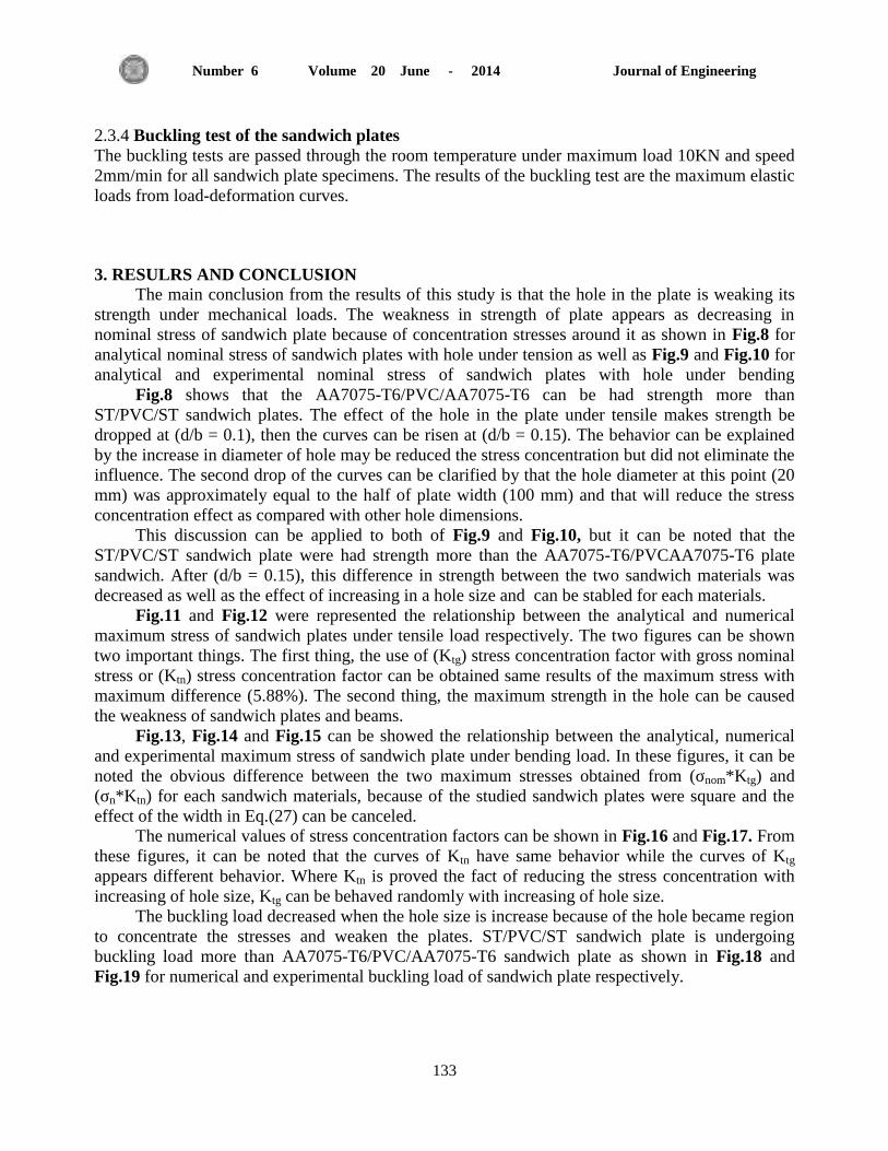
Journal of Engineering Volume 20 June - 2014 Number 6
133
2.3.4 Buckling test of the sandwich plates
The buckling tests are passed through the room temperature under maximum load 10KN and speed
2mm/min for all sandwich plate specimens. The results of the buckling test are the maximum elastic
loads from load-deformation curves.
3. RESULRS AND CONCLUSION
The main conclusion from the results of this study is that the hole in the plate is weaking its
strength under mechanical loads. The weakness in strength of plate appears as decreasing in
nominal stress of sandwich plate because of concentration stresses around it as shown in Fig.8 for
analytical nominal stress of sandwich plates with hole under tension as well as Fig.9 and Fig.10 for
analytical and experimental nominal stress of sandwich plates with hole under bending
Fig.8 shows that the AA7075-T6/PVC/AA7075-T6 can be had strength more than
ST/PVC/ST sandwich plates. The effect of the hole in the plate under tensile makes strength be
dropped at (d/b = 0.1), then the curves can be risen at (d/b = 0.15). The behavior can be explained
by the increase in diameter of hole may be reduced the stress concentration but did not eliminate the
influence. The second drop of the curves can be clarified by that the hole diameter at this point (20
mm) was approximately equal to the half of plate width (100 mm) and that will reduce the stress
concentration effect as compared with other hole dimensions.
This discussion can be applied to both of Fig.9 and Fig.10, but it can be noted that the
ST/PVC/ST sandwich plate were had strength more than the AA7075-T6/PVCAA7075-T6 plate
sandwich. After (d/b = 0.15), this difference in strength between the two sandwich materials was
decreased as well as the effect of increasing in a hole size and can be stabled for each materials.
Fig.11 and Fig.12 were represented the relationship between the analytical and numerical
maximum stress of sandwich plates under tensile load respectively. The two figures can be shown
two important things. The first thing, the use of (Ktg) stress concentration factor with gross nominal
stress or (Ktn) stress concentration factor can be obtained same results of the maximum stress with
maximum difference (5.88%). The second thing, the maximum strength in the hole can be caused
the weakness of sandwich plates and beams.
Fig.13, Fig.14 and Fig.15 can be showed the relationship between the analytical, numerical
and experimental maximum stress of sandwich plate under bending load. In these figures, it can be
noted the obvious difference between the two maximum stresses obtained from (σnom*Ktg) and
(σn*Ktn) for each sandwich materials, because of the studied sandwich plates were square and the
effect of the width in Eq.(27) can be canceled.
The numerical values of stress concentration factors can be shown in Fig.16 and Fig.17. From
these figures, it can be noted that the curves of Ktn have same behavior while the curves of Ktg
appears different behavior. Where Ktn is proved the fact of reducing the stress concentration with
increasing of hole size, Ktg can be behaved randomly with increasing of hole size.
The buckling load decreased when the hole size is increase because of the hole became region
to concentrate the stresses and weaken the plates. ST/PVC/ST sandwich plate is undergoing
buckling load more than AA7075-T6/PVC/AA7075-T6 sandwich plate as shown in Fig.18 and
Fig.19 for numerical and experimental buckling load of sandwich plate respectively.

Journal of Engineering Volume 20 June - 2014 Number 6
134
When the deformation shape modes are discussed, the solid plates have different forth
deformation shape mode for the two sandwich materials shown in Fig.15 a and b.
While the deformation shape modes are differed and changed for sandwich plates with hole
but they remain the same in each sandwich materials as shown in Fig.16 a and b. The hole not only
causes a decrease in resistance but is changing the deformation shape modes of the sandwich plate
since each sandwich materials varies in response the deformation shape modes are differed for each
one because of the different in faces materials.
The comparisons between the theoretical, numerical and experimental results are shown in
Fig.17 and Fig.18.
REFFRENCES
Ali, V. S. and Masood, M.,2010, Parametric Studies on the FEM Analysis of Foam Core Sandwich
Panels with Holes, 5th National Congress on Civil Engineering, Ferdowsi University of Mashhad,
Mashhad, Iran, May 4-6, 2010.
Ansel, C. U., 1999, Stresses in Plates and Shells, 2nd edition, New York: McGraw-Hill,
Berthelot, J.-M, 2010, Mechanics of Composite Materials and Structures, by Springer.
Daniel, G., Suong, V. H. and Stephen W.T., 2003, Composite Materials Design and Application,
2nd Edition, by CRC Press LLC.
Erdogan, M. and Ibrahim, G., 2006,The Finite Element Method and Applications in Engineering
Using ANSYS, by Springer.
Podruzhin, E.G., and Ryabchikov, P.E., 2004, Bending of Anisotropic plates with Stress
Concentrations, by IEEEXplore
Qing-Sheng, Y. and Wilfried, B., 2004, Effective Stiffness and Microscopic Deformation of an
Orthotropic Plate Containing Arbitrary Holes, Computers and Structures, Vol.82, p.p:2301–2307.
Saeed, M., 1999, Finite Element Analysis Theory and Application with ANSYS, by Shashi Bhushan
Patel
Springer, G.S. and Kolla'r, L.P., 2003, Mechanics of Composite Structures, by Cambridge
University Press.
Walter, D. P., 1997, Peterson's Stress Concentration Factor, 2nd
edition, by John Wiley & Sons.
Wang, C.M., Reddy, J.N. and Lee, K.H., 2000, Shear Deformable Beams and Plates Relationships
with Classical Solution, 1st Edition, by Elsevier.

Journal of Engineering Volume 20 June - 2014 Number 6
135
NOMENCLAUTURE
shear strain components of middle-plane in (z) directions respectively.
,
strain components of middle-plane in (x, y) directions respectively.
.
curvatures components of the middle-plane.
, MPa.
, MPa.
, rotation of the cross section in the x-y and x-z planes respectively.
, : extensional stiffness, the coupling stiffness, and the bending stiffness.
.
, mm.
b: beam and plate width, mm.
.
Ef, Ec: Young modulus of skin and core respectively, Pa.
.
Gf, Gc: shear modulus of skin and core respectively, Pa.
thickness of lower and upper skins respectively, .
, .
.
.
, , N.
.
, q: external load.
: middle-plane displacement components along (x, y and z) directions respectively , mm.

Journal of Engineering Volume 20 June - 2014 Number 6
136
Figure 1. Sandwich materials.
Figure 2. Sandwich plate under bending load.
Figure 3. Mesh of solid sandwich plate.
Figure 4. Mesh of sandwich plate with hole under tension and buckling.

Journal of Engineering Volume 20 June - 2014 Number 6
137
Figure 5. Mesh of sandwich plate with hole under bending.
(a) (b)
(c)
Figure 6. Tensile test curves: (a) Steel, (b) AA7075-T6, (c) PVC.
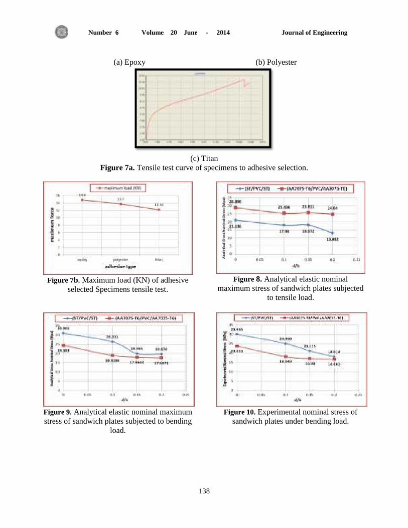
Journal of Engineering Volume 20 June - 2014 Number 6
138
(a) Epoxy (b) Polyester
(c) Titan
Figure 7a. Tensile test curve of specimens to adhesive selection.
Figure 7b. Maximum load (KN) of adhesive
selected Specimens tensile test.
Figure 8. Analytical elastic nominal
maximum stress of sandwich plates subjected
to tensile load.
Figure 9. Analytical elastic nominal maximum
stress of sandwich plates subjected to bending
load.
Figure 10. Experimental nominal stress of
sandwich plates under bending load.

Journal of Engineering Volume 20 June - 2014 Number 6
139
Figure 11. Analytical maximum stresses of
sandwich plates under tensile load.
Figure 12. Numerical maximum stress of
sandwich plates under tensile load.
Figure 13. Analytical maximum stresses of
sandwich plates under bending load.
Figure 14. Experimental maximum stresses of
sandwich plates under bending load.
Figure 15. Numerical maximum stress of sandwich plates under bending load.
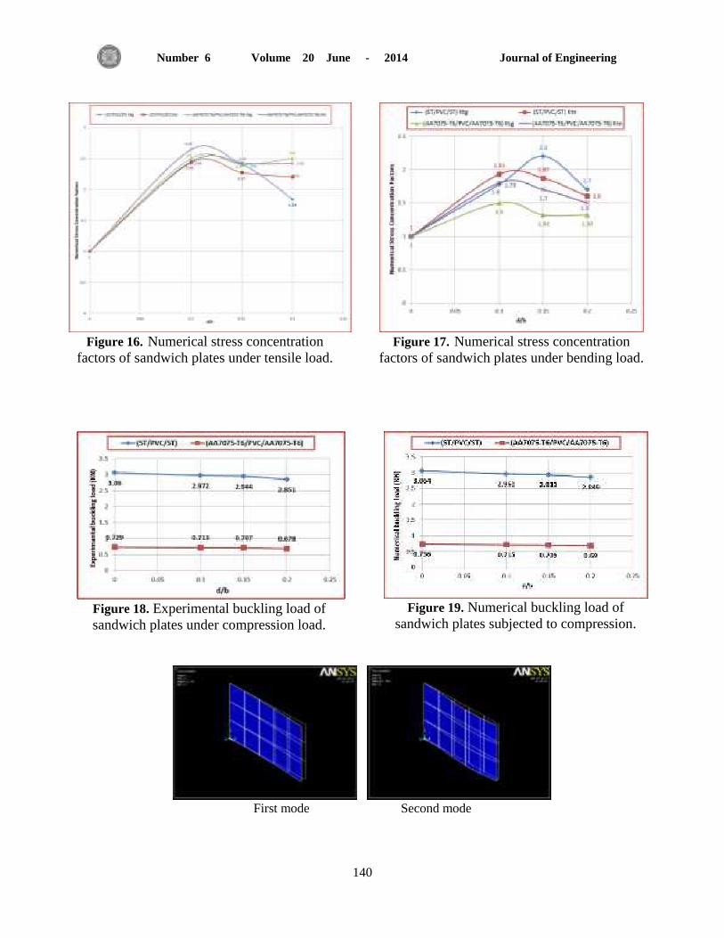
Journal of Engineering Volume 20 June - 2014 Number 6
140
Figure 16. Numerical stress concentration
factors of sandwich plates under tensile load.
Figure 17. Numerical stress concentration
factors of sandwich plates under bending load.
Figure 18. Experimental buckling load of
sandwich plates under compression load.
Figure 19. Numerical buckling load of
sandwich plates subjected to compression.
First mode Second mode
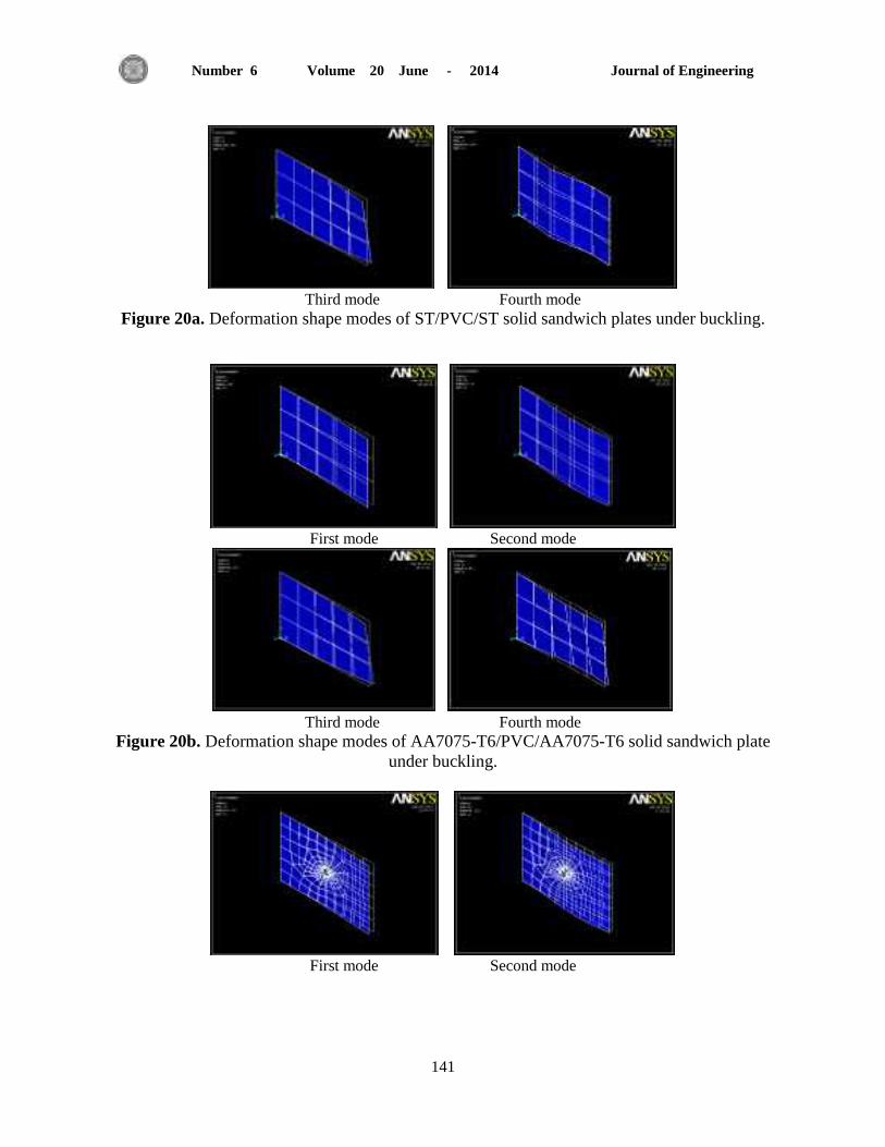
Journal of Engineering Volume 20 June - 2014 Number 6
141
Third mode Fourth mode
Figure 20a. Deformation shape modes of ST/PVC/ST solid sandwich plates under buckling.
First mode Second mode
Third mode Fourth mode
Figure 20b. Deformation shape modes of AA7075-T6/PVC/AA7075-T6 solid sandwich plate
under buckling.
First mode Second mode

Journal of Engineering Volume 20 June - 2014 Number 6
142
Third mode Fourth mode
Figure 21a. Deformation shape modes of ST/PVC/ST sandwich plate with hole under buckling.
First mode Second mode
Third mode Fourth mode
Figure 21b. Deformation shape modes of AA7075-T6/PVC/AA7075-T6 sandwich plate with hole
under buckling.
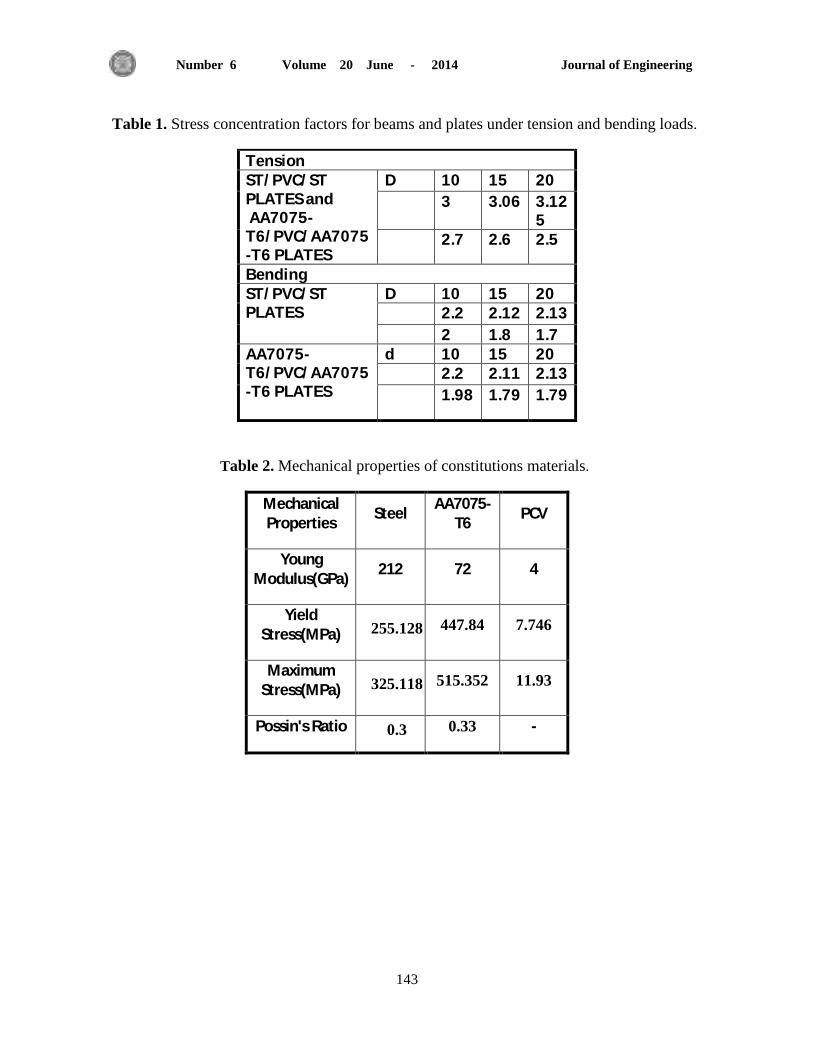
Journal of Engineering Volume 20 June - 2014 Number 6
143
Table 1. Stress concentration factors for beams and plates under tension and bending loads.
Tension ST/PVC/ST PLATES and AA7075-T6/PVC/AA7075-T6 PLATES
D 10 15 20
3 3.06 3.125
2.7 2.6 2.5
Bending ST/PVC/ST PLATES
D 10 15 20 2.2 2.12 2.13
2 1.8 1.7 AA7075-T6/PVC/AA7075-T6 PLATES
d 10 15 20 2.2 2.11 2.13
1.98 1.79 1.79
Table 2. Mechanical properties of constitutions materials.
Mechanical Properties
Steel AA7075-
T6 PCV
Young Modulus(GPa)
212 72 4
Yield Stress(MPa) 255.128 447.84 7.746
Maximum Stress(MPa) 325.118 515.352 11.93
Possin's Ratio 0.3 0.33 -

Journal of Engineering Volume 20 June - 2014 Number 6
144
Kinetics of the Saponification of Mixed Fats Consisting of Olein and Stearin
Dr. Raghad Fareed Kassim Almilly
Lecturer
Department of Chemical Engineering
College of Engineering - Baghdad University
Email: [email protected]
ABSTRACT
This research presents the kinetics of the saponification reaction using mixed fats of olein
and stearin [in the ratio (3:1)] with NaOH solution . In this reaction , excess solution of NaOH
was used to ensure the reaction being irreversible . Three parameters were varied to show their
effects on the reaction rate .They are : percentage excess of NaOH solution (10 % - 100 %) ,
temperature (100-150)oC , and stirring speed (400-1100) rpm. It was noticed that increasing the
percentage excess of NaOH solution enhances the rate of reaction while increasing temperature
decreases the reaction rate since it is exothermic reaction. Increasing stirring speed also
improves the reaction rate because it is mass transfer controlled .Calculations of the activation
energy and the frequency factor were also performed.
A new mathematical model for calculation of the reaction – rate constant was derived . It is
shown that a good approximation was obtained between the experimental and calculated values
of the reaction – rate constant k .
Key words: kinetics, saponification reaction , mixed fats , olein and stearin , mathematical
model.
االولين والستيارينحركية تفاعل الصوبنة لمسيج من زيتي
د. رغذ فريذ قاسم الملي
يذسط قسى انهذست انكبوت
خبيعت بغذاد -كهت انهذست
الخالصة
( [ يع يحهىل هذسوكسذ 1:1قذو هزا انبحث حشكت حفبعم انصىبت ببسخخذاو خهظ ي صخ االون وانسخبس ] بسبت )
انصىدىو .سخخذو ف هزا انخفبعم سبت صائذة ي يحهىل هذسوكسذ انصىدىو نضب كى انخفبعم غش عكس . حى حغش
% ( , 100 -% 10شعت انخفبعم وهى سبت انضبدة انئىت نحهىل هذسوكسذ انصىدىو )ثالثت عىايم نبب حأثشهى عهى س
( دوسة/ دققت. وقذ نىحظ ا صبدة سبت انضبدة انئىت نحهىل 1100-000( و , و سشعت انخهظ )150-100دسخت انحشاسة )
. انخفبعم أله حفبعم ببعث نهحشاسةانحشاسة حقهم سشعت هذسوكسذ انصىدىو حؤدي انى صبدة سشعت انخفبعم بب صبدة دسخت
كزنك حى احخسبة خ سطش عههب اخقبل انبدة.أضب صبدة سشعت انخهظ حؤدي انى صبدة سشعت انخفبعم أله ي انخفبعالث ان
ب وخىد حقبسة خذ ب انقى طبقت انخشظ وعبيم انزبزبت. حى اشخقبق ىرج سبض خذذ نحسبة ثببج سشعت انخفبعم . نقذ ح
انعهت وانقى انحسىبت نثببج سشعت انخفبعم.
.انحشكت , حفبعم انصىبت , يضح ي انضىث , االون وانسخبس , ىرج سبض :الرئيسيةالكلمات

Journal of Engineering Volume 20 June - 2014 Number 6
145
1. INTRODUCTION
It has been said that the use of soap is a gauge of the civilization of a nation . Many literature
were published in the field of saponification of various fats and fatty acids.Frost and
Schwemer,1952. had studied the differential rate equations for the kinetics of competitive
consecutive second – order reactions . Measurements of the rate of saponification of ethyl
adipate and ethyl succinate were used to verify the theoretical approach . Newberger and
Kadlec , 1973 had studied the kinetics of the saponification of diethyl adipate between 302K and
358K , for both stirred and tubular reactors . They had suggested numerical search method to
verify the proposed model. Vicente, et al., 2006. Studied the kinetics of Brassica Carinata oil
methanolysis . They found that the methanolysis reaction can be described as a pseudo –
homogeneous catalyzed reaction , following a second – order mechanism for the forward and
reverse reactions . They also found that higher temperature and catalyst concentrations increased
the reaction rates . Appleton Appleton, 2007, had published a handbook of soap manufacture .
He had made a review of oils and fats and their saponification . He had presented the steps of
soap – making even soap perfuming and molding . Lab. Report , 2012, was presented to
determine the order, rate constant , activation energy , and pre – exponential factor for the
reaction of ethyl acetate with base using conductance measurements. An experimental study of
the reaction kinetics of a simple homogenous liquid – phase system was published , Chem. Eng.
Lab. , 2013. The reaction kinetics of the saponification of isopropyl acetate with sodium
hydroxide was presented.
There are some aspects of interest still need to be studied . Determination the order , rate
constant and many other parameters in the saponification kinetics are of great importance . The
objective of this research is to study the parameters that affect saponification reaction. These
parameters can be used to model the reaction to a large – scale applications , enhance an existed
production and adopt an optimum set of parameters for a new production .
2. THEORITICAL ASPECTS
2.1 Saponification Reaction
The saponification reaction is of the form
Fat + sodium hydroxide = soap + glycerol
The fat used is a mixture of olein and stearin with a ratio (3:1) . These fats are the most important
ones from a soap –maker's point of view , Appleton , 2007 . Using (3:1) ratio ensures the
product (soap) to be soft enough (by using olein ) and solid enough (by using stearin ) for toilet
use. Appleton had published various types of fats and fatty acids . Olein (derived from olive and
cotton – seed oil ) is saponified according to the following reaction :
C3H5(C18H33O2)3 + 3NaOH = 3NaO2C18H33 + C3H5(OH)3
olein sodium sodium oleate glycerol
hydroxide ( soap )
Stearin ( derived from tallow ) is saponified according to the following reaction :
C3H5(C18H35O2)3 + 3NaOH = 3NaO2C18H35 + C3H5(OH)3

Journal of Engineering Volume 20 June - 2014 Number 6
146
stearin sodium sodium stearate glycerol
hydroxide ( soap )
Therefore; the chemical equation for saponification reaction can be represented by :
A + B = R + S
Where A , B refer to the reactants ( fat and caustic soda ) and R , S refer to the products ( soap
and glycerol). The reaction rate is , Smith ,1981.
rA = k CA CB – k ' CR CS
where : k is the forward reaction – rate constant
k' is the backward reaction – rate constant
represents the molar concentration of the specified substance in (mol / l ) C
If an excess of NaOH solution is added , the reaction will be considered as irreversible , such as
Smith , 1981.
A + B → R + S
and the rate equation will be :
rA = k CA CB
Since the reaction is in liquid phase (constant volume),Smith , 1981.
rA = - dCA / dt = k CA CB (1)
2.2 Kinetics of Saponification Reaction
The kinetics study of this work consists of the following:
(i) Determination of the order of the reaction
(ii) Determination of the rate constant
(iii) Determination of the activation energy
(iv) Determination of the frequency factor or ( pre - exponential ) factor
under the variation of three parameters : the percentage excess of NaOH , the temperature and
the stirring speed.
The basic relation in kinetics study is the concentration –time relation of the reactants. The
concentration – time data can be detected using titration of samples and refractive indices
determination.
2.3 Modeling the Rate Equation
Previous works that studied the kinetics of saponification reaction had either simplified the
solution of the differential equation by approximation, Lab. Report, 2012 or solved it by
iteration , Newberger, and Kadlec , 1973.

Journal of Engineering Volume 20 June - 2014 Number 6
147
In this work, the differential equation will be dealt as it is and solved with somewhat tedious
integration method , as follows:
rA = - dCA / dt = k CA CB (1)
The fractional conversion , xA , is defined as :
xA = ( CAo – CA ) / CAo
Differentiation:
- dCA / dt = CAo dxA / dt (2)
CA and CB are defined through xA as:
CA = CAo (1 – xA) (3)
CB = CBo – 3 (CAo - CA ) (4)
Where Eq. (3) is the stoichiometric factor and CAo , CBo are the initial concentrations of
reactants A and B , respectively. Dividing Eq. (4) by CAo yields:
CB / CAo = CBo / CAo – 3( CAo - CA ) / CAo
CB / CAo = CBo / CAo – 3 xA
or CB = CBo – 3 xA CAo (5)
Substituting Eqs. (2) , (3) , and (5) into Eq. (1) , yields :
CAo dxA / dt = k CAo (1 – xA) (CBo –3xACAo)
Dividing by CAo leads to:
dxA/dt= k (1–xA) (CBo–3xACAo) (6)
Separating the variables , yields :
dxA/(1–xA)(CBo–3xACAo)=kdt (7)
Integrating from t = 0 , xA = 0 to t = t and xA = xA yields :
∫
( )( )
∫
(8)
Using fractional integration :
( )( )
(9)
Multiplying by ( 1- xA ) (CBo – 3 xA CAo), yields :
1 = E (CBo–3 xA CAo) + F (1–xA) (10)
1 = E CBo - 3 E xA CAo + F – F xA
Equating the coefficients of xAo :
1 = E CBo + F (11)
Equating the coefficients of xA1 :

Journal of Engineering Volume 20 June - 2014 Number 6
148
0 = - 3 E CAo - F (12)
Therefore; F = - 3 E CAo
Substituting into Eq. (11) , yields:
1 = E CBo – 3 E CAo (13)
or E = 1 / (CBo−3CAo) (14)
and F = - 3 CAo / (CBo−3CAo) (15)
Substituting Eqs. (14) and (15) into Eq. (9) , yields :
( ) ( )
( ) ( )
( ) ( )
and
∫
( )(
)
(
)∫
( )
(
) ∫
(
)
Substituting into Eq. (8) , yields :
(
)[∫
( )
∫
(
)
] ∫
Integrating , yields :
(
)[ ( ) (
)]
or
( )*
+
so *
+
( )
is the proposed model . This model can be verified through the experimental work .
3. EXPERIMENTAL WORK
3.1 Apparatus
The apparatus used in this work consists of 1000 ml- beaker (modified with lower tapped glass
tube to ensure the separation of the lower glycerol layer from the upper soap layer ) , hot plate
stirrer (RLABINCO , Model L-81,The Netherlands) . It's provided with two nobs ; one for
controlling the temperature (100 - 150 ) oC and the other for controlling the stirring speed (400 –
1100 ) rpm . The apparatus also consists of thermometer ( for measuring the actual temperature
of the reacting mixture ) , various glassware for preparation of solutions and titration of samples ,

Journal of Engineering Volume 20 June - 2014 Number 6
149
Refractometer ( Model Optika , no. 2WAJ SN 281006 , Italy ) . The refractometer is used to
measure the refractive index of the samples .
3.2 Materials Materials used are : olein and stearin fats ( source: Republic Company of Vegetable Oils) ,
sodium hydroxide (NaOH) solution (Aldrich mark) standardized against standard hydrochloric
acid (HCl) solution (commercial grade ) , Vogel , 1961. , saturated solution of brine , distilled
water .
3.3 Procedure
The procedure consists of the following steps:
1-Weighing the required amounts of fats then transferring them to the beaker.
2- Switch on the heater and stirrer and fixing them on certain values.
3-Adding an excess amount of sodium hydroxide solution with changeable percentage excess
(10% - 100%).
4-Beginning the reaction for specified CAo and CBo .
5-Taking a sample every 5-10 minutes till the end of the reaction (soap formation). Samples
were titrated against standard HCl solution using methyl orange as an indicator ,Vogel , 1961.
also the refractive indices were measured for these samples.
6-Adding distilled water to cool the reaction mixture and to suppress the froth of the soap when
necessary .
7-Adding saturated brine solution to facilitate the separation of layers.
8-The soap was then molded, dried, and used.
4. RESULTS AND DISCUSSION
Experiments were performed at different levels of the three parameters ( percentage excess of
NaOH solution (10%-100%) , temperature (100-150) oC , and stirring speed (400-1100) rpm .
Each experiment depicted a concentration – time curve . To calculate the order of the reaction
and the rate constant , the differential method was adopted . This was achieved by calculating
different slopes at different concentrations of tangent points of the concentration – time curve .
These slopes represented dCA/dt (reaction rate with respect to the limiting reactant A) . Taking
the natural logarithms for each dCA/dt and CA , then drawing data gives a straight line of slope
equal nA ( the order of the reaction with respect to A ) and of intercept equals ln k. The inverse
of ln k gives the experimental value of k (reaction – rate constant).Table 1 shows a sample of
concentration –time data for both reactant A and reactant B , with the refractive indices and
conversions for run no.(4).Fig.1 shows the concentration - time curve of reactant A. The curve
shows decreasing of CA with time until complete consumption. This is because reactant A is the
limiting reactant . Table 2 shows data for the slopes determined at the tangent points of Fig. 1.
The data illustrate decreasing of slopes' magnitudes for the points . This means decreasing the
rate of reaction with the concentration decrease, which indicates the progress of reaction. Table
3 shows the logarithm of the rate of reaction ln (-dCA/dt) with the logarithm of the concentration
lnCA. Fig. 2 depicted these data. It was shown that the order of reaction with respect to A is
approximately 1. The value of the rate constant was also determined. These calculations were
also done for the excess reactant B ( NaOH solution ) to find the order of the reaction with

Journal of Engineering Volume 20 June - 2014 Number 6
150
respect to it (nB). Fig. 3 traces the concentration - time profile of reactant B. It is clear that
reactant B dose not tend to complete consumption , since it is the excess reactant. Table 4
shows (- dCB / dt) versus CB data . Similarly , the rate of reaction decreased with decrease in
concentration .Table 5 shows the variation of ln (-dCB/dt) with ln CB .Fig. 4 traces ln(-dCB/dt)
against lnCB. The relation is linear with slope equals nB. Again the value of nB is about 1 .
Experimental results showed that the order of reaction for each reactant nA , nB ≈1 , so the
overall order of reaction was second order . This result agreed with the fact that most of
esterification reactions are second order .Saponification reaction is an example of these
reactions. It was also noticed that the values of the refractive index RI decreases as the
conversion increases. After approximately 50% conversion, the values of RI increases again. To
explain this behavior, the relationship between RI and the density must be noticed. RI is a
physical property that inversely proportional to density. As NaOH solution was added to the
fat , the density of the fat is increased (RI is decreased).When the soap was produced the density
again decreased (RI is increased). The concentration - time data were substituted in the
mathematical model using conversions instead of concentrations.
Fig. 5 shows the relation between the expression ln D (*
+
) and time.
The relation is linear with slope equal kcalc . The calculated values of the reaction-rate
constant were somewhat deviate from the experimental ones. It was noticed that k values
obtained from the mathematical model were overestimated when the percentage excess of NaOH
solution were too low or too high. At medium levels of % excess of NaOH solution the
calculated values of k were underestimated. This can be discussed as follows: at low values of
% excess of NaOH solution , the reaction rate decreases because of the decreased concentration
of NaOH giving reduced values of reaction –rate constant kexp .This makes the calculated
values be higher . High values of % excess of NaOH solution reduce the number of reacting
molecules , as a result of hindering their movement , causing reduced values of kexp again. This
also makes kcalc be higher. The average error between experimental and calculated values of k
was calculated by the following equation:
Av. Error =∑ (
)
Where N is the number of runs . The average error was approximately 20%. This figure may be
accepted because the experimental errors were thought to be lumped within it . Fortunately; the
underestimated values of kcalc resulted from the mathematical model allow safe design and
simulation calculations.
Fig. 6 shows the effect of increasing the percentage excess of NaOH solution on reaction – rate
constants ( kexp and kcalc ) . The calculated values trace lower curve than experimental ones
except at approximately 100% excess . Evidently, increasing NaOH solution enhances the rate
of reaction because it suppresses the backward reaction according to Le Chatelier rule .

Journal of Engineering Volume 20 June - 2014 Number 6
151
The effect of temperature is presented in Fig. 7 . The natural logarithms of k is plotted against
the reciprocal of the absolute temperature . This figure shows a linear relation between ln k and
1/T as it was predicted by Arrhenius.
(
)
where the slope (
) represents the negative value of the activation energy divided by the
universal perfect-gas law constant . The intercept of the plot ( ln Ao ) determines the frequency
factor . The values of the activation energy and the frequency factor were found to be as follows:
Ea exp = -20.44 J.mol-1
and
Aoexp =9.8358×10
-5 l.mol
-1.min
-1
While Ea calc = -4.67 J.mol-1
and
Aocalc = 6.2×10
-3 l.mol
-1.min
-1
The experimental and calculated values are different by an order of magnitude which is
attributed to the experimental error .The value of the activation energy is rather low. This
indicates that the reaction is fast since the activation energy represents the energy barrier that
molecules must gain to reach the final product .
Fig. 8 shows the effect of stirring speed upon the rate constants. It is clear that the effect of
stirring is considerable on the reaction rate. This leads to the conclusion that the reaction is mass
- transfer controlled. This viewpoint agrees well with the notation of underestimated values of
kexp at high values of percentage excess of NaOH solution. Therefore; increasing stirring speed
enhances the reaction rate. However, there is a constraint limited by the soap - froth rising .If the
values of kexp were normalized (i.e. making the total increase in kexp corresponds 100% ) as
shown in Table 6. This was done for the runs that have only the excess ratio varied , i.e. the
temperature and stirring speed were fixed . The normalization shows that percentage excess over
50% has less effect on the value of kexp than the percentage excess below 50%. This may be
attributed to the hindrance of reacting molecules by the NaOH molecules which confirms the
mass- transfer control on the reaction.
5. CONCLUSIONS
- The % excess of NaOH solution plays an important role in the saponification reaction. 88% of
increased value of the rate constant k can be achieved at 50% excess . Adding more solution of
NaOH seems to be unnecessary and costing .
- The saponification reaction is mass – transfer controlled and stirring speed appears as an
effective parameter , although excessive stirring may raise the froth of the soap .
- The derived mathematical model is adequately described the system especially at moderate
values of % excess of NaOH solution .
- The mathematical model can be applied to scale – up the laboratory batch reactor to a large –
scale continuously stirred tank reactor (CSTR).

Journal of Engineering Volume 20 June - 2014 Number 6
152
REFERENCES
- Appleton, H.A.,2007, The Handbook of Soap Manufacture , Scott , Greenwood & Son ,
London.
- Chemical Engineering Laboratory,2013, Saponification of Isopropyl Acetate with Sodium
Hydroxide, (Internet Document).
- Frost, A. A., and Schwemer, W. C.,1952, The Kinetics of Competitive Consecutive Second
Order Reactions:The saponification of Ethyl Adipate and of EthylSuccinate, Journal of
American Chemical Society, Vol.74, No.5, PP. 1268-1273.
-Laboratory Report, 2012 , The Kinetics of the Saponification of Ethylacetate , (Internet
Document).
- Newberger , M. R., and Kadlec , R. H.,1973, Kinetics of the Saponification of Diethyl Adipate,
American Institute of Chemical Engineers Journal ,Vol.19, No.5 , PP. 1272 - 1275 .
- Smith, J. M., 1981, Chemical Engineering Kinetics , 3rd
ed. , Mc-Graw Hill.
- Vicente,G. , Martinez, M. , and Aracil, J., 2006, Kinetics of Brassica Carinata Oil
Methanolysis , Energy Fuels ,Vol. 20,No.4 , PP. 1722 – 1726.
- Vogel, A.I.,1961, Quantitative Inorganic Analysis , 3rd
ed. , Longmans.
NOMENCLATURE
A limiting reactant (fat)
Ao frequency factor (l . mol
-1 . min
-1)
B excess reactant (NaOH solution)
C concentration (mol . l-1
)
D expression ( *
+
)
E arbitrary constant
Ea activation energy (J . mol-1
)
F arbitrary constant
k forward reaction-rate constant ( l . mol-1
. min-1
)
k' backward reaction-rate constant(l . mol-1
. min-1
)
N number of runs
n order of reaction
R product 1 (soap)
Rg universal gas-law constant ( 8.314 J. mol-1
. K-1
)
RI refractive index
r reaction rate (mol . l-1
. min-1
)

Journal of Engineering Volume 20 June - 2014 Number 6
153
rpm revolution per minute
S product 2 (glycerol)
T absolute temperature (K)
t time (min)
x fractional conversion (-)
Subscripts
o initial ( CAo initial conc. of reactant A)
Table 1. Concentration – time data of reactant A (fat) with refractive indices and conversions for
run no.(4) [%excess=50 , Temp.=100oC , rpm=400].
Figure 1.Concentration-time profile with respect to
reactant A (fat) of run no.(4) [% excess=50 , Temp.=100oC , rpm=400].
0
1
0 10 20 30 40 50
Co
nc.
of
fat
, CA
(m
ol/
l)
time , t (min
t
(min)
CA
(mol . l-1
)
RI
(-)
xA
(-)
CB
(mol . l-1
)
0 0.3119 1.468 0 2.844
10 0.0815 1.42 0.7387 2.1528
20 0.0789 1.412 0.7471 2.1449
30 0.0577 1.428 0.8151 2.0813
35 0.0471 1.472 0.8490 2.0496
40 0.0259 1.52 0.917 1.986

Journal of Engineering Volume 20 June - 2014 Number 6
154
Table 2.Rate of reaction with respect to reactant A(slope) versus the concentration of A of run
no.(4) [% excess=50 , Temp.=100oC , rpm=400].
Slope (dCA/dt) CA
-0.0115 0.22
- 0.0086 0.20
-0.0063 0.16
-0.0043 0.11
Table 3.Logarithm of reaction rate versus logarithm of concentration of reactant A (fat) of run
no.(4) [% excess=50 , Temp.=100oC , rpm=400].
ln(- dCA/dt) ln CA
-4.4654 -1.5141
-4.7560 -1.6094
-5.0672 -1.8326
-5.4491 -2.2073
Figure 2.The linear relation between ln(-dCA/dt) and ln CA gives the order of reaction with
respect to reactant A. nA(slope) and ln kexp (intercept) of run no. (4) [% excess=50 ,
Temp.=100oC, rpm=400].
y = 1.342x - 2.5311
-6
-5
-4
-3
-2
-1
0-2.5 -2 -1.5 -1 -0.5 0
ln(-
dC
A/d
t)
lnCA
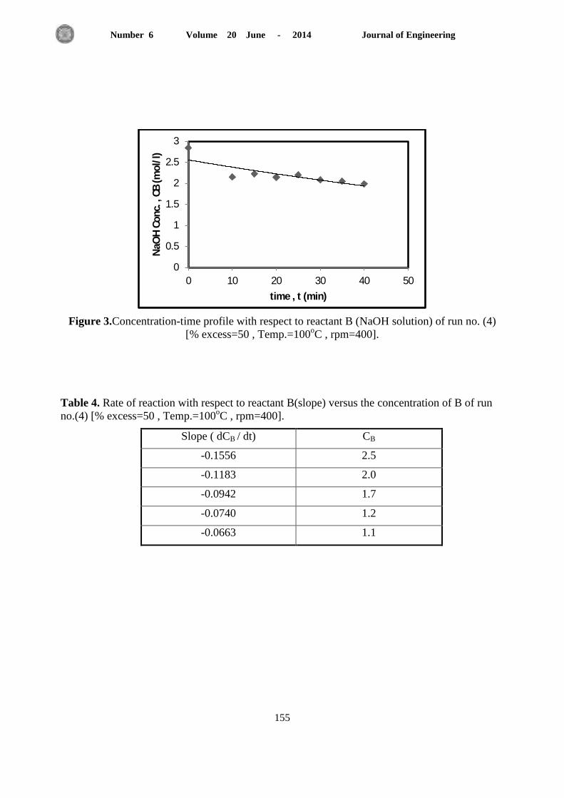
Journal of Engineering Volume 20 June - 2014 Number 6
155
Figure 3.Concentration-time profile with respect to reactant B (NaOH solution) of run no. (4)
[% excess=50 , Temp.=100oC , rpm=400].
Table 4. Rate of reaction with respect to reactant B(slope) versus the concentration of B of run
no.(4) [% excess=50 , Temp.=100oC , rpm=400].
Slope ( dCB / dt) CB
-0.1556 2.5
-0.1183 2.0
-0.0942 1.7
-0.0740 1.2
-0.0663 1.1
0
0.5
1
1.5
2
2.5
3
0 10 20 30 40 50
NaO
H C
on
c. ,
CB
(m
ol/
l)
time , t (min)
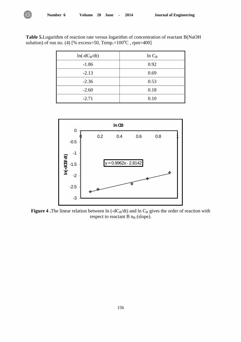
Journal of Engineering Volume 20 June - 2014 Number 6
156
Table 5.Logarithm of reaction rate versus logarithm of concentration of reactant B(NaOH
solution) of run no. (4) [% excess=50, Temp.=100oC , rpm=400]
Figure 4 .The linear relation between ln (-dCB/dt) and ln CB gives the order of reaction with
respect to reactant B nB (slope).
y = 0.9962x - 2.8142
-3
-2.5
-2
-1.5
-1
-0.5
0
0 0.2 0.4 0.6 0.8 1
ln(-
dC
B/d
t)
ln CB
ln(-dCB/dt) ln CB
-1.86 0.92
-2.13 0.69
-2.36 0.53
-2.60 0.18
-2.71 0.10

Journal of Engineering Volume 20 June - 2014 Number 6
157
Figure 5.The proposed model shows linearity between ln D (*
+
) and time
with CAo and CBo of run no. (4) the slope determines kcalc.
Figure 6.The effect of % excess of NaOH solution on the experimental and calculated reaction -
rate constants kexp and kcalc.
y = 0.0221x + 0.6511
0
0.2
0.4
0.6
0.8
1
1.2
1.4
1.6
1.8
0 10 20 30 40 50
ln
D
time , t (min
0
0.02
0.04
0.06
0.08
0.1
0.12
0.14
0 50 100 150
reac
tio
n r
ate
co
nst
ant
k ,
l.m
ol-
1.m
in-1
percentage excess of NaOH solution
kexp
kcalc
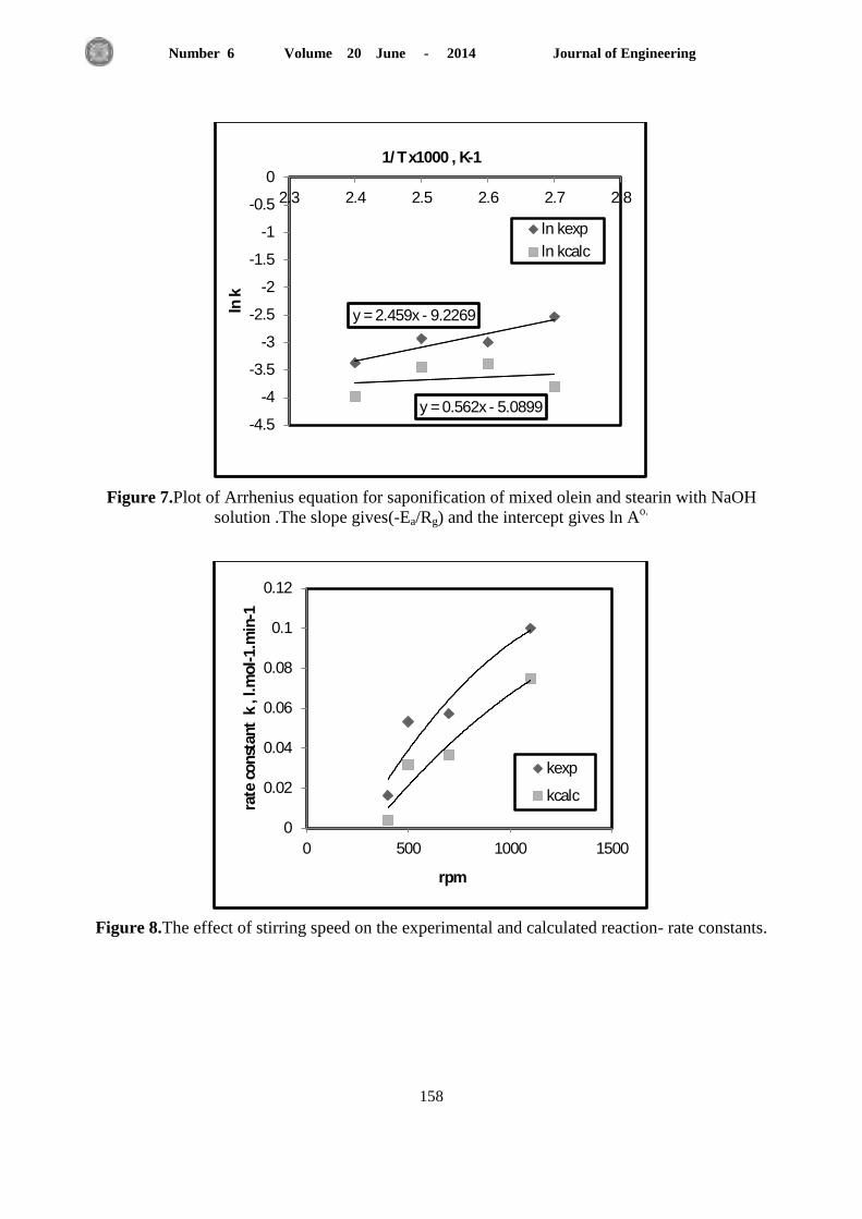
Journal of Engineering Volume 20 June - 2014 Number 6
158
Figure 7.Plot of Arrhenius equation for saponification of mixed olein and stearin with NaOH
solution .The slope gives(-Ea/Rg) and the intercept gives ln Ao.
Figure 8.The effect of stirring speed on the experimental and calculated reaction- rate constants.
y = 2.459x - 9.2269
y = 0.562x - 5.0899 -4.5
-4
-3.5
-3
-2.5
-2
-1.5
-1
-0.5
0
2.3 2.4 2.5 2.6 2.7 2.8
ln k
1/T x1000 , K-1
ln kexp
ln kcalc
0
0.02
0.04
0.06
0.08
0.1
0.12
0 500 1000 1500
rate
co
nst
ant
k ,
l.m
ol-
1.m
in-1
rpm
kexp
kcalc

Journal of Engineering Volume 20 June - 2014 Number 6
159
Table 6.The effect of % excess of NaOH solution on the value of kexp
%excess Temp.
(oC)
rpm kexp
(l.mol-1
. min-1
)
% increase in
kexp
10 100 400 0.0164 0
50 100 400 0.0716 88
100 100 400 0.0791 100

Journal of Engineering Volume 20 June - 2014 Number 6
061
Analysis and Control of PWM Buck-Boost AC Chopper Fed Single-Phase
Capacitor Run Induction Motor
Prof. Dr. Jafar H. Alwash Asst. Prof. Dr. Turki K. Hassan Shams W. Kamel
Engineering College
Baghdad University
Engineering College
Al-Mustansiriya University Engineering College
Baghdad University E-mail: [email protected] E-mail: [email protected]
ABSTRACT
Single phase capacitor-run induction motors (IMs) are used in various applications such as
home appliances and machine tools; they are affected by the sags or swells and any fault that can
lead to disturb the supply and make it produce rms voltage below or above the rated motor
voltage, which is 220V. A control system is designed to regulate the output voltage of the
converter irrespective to the variation of the load and within a specific range of supply voltage
variation. The steady-state equivalent circuit of the Buck-Boost chopper type AC voltage
regulator, as well as the analysis of this circuit are presented in this paper. Switching device for
the regulator is an IGBT Module. The proposed chopper uses pulse width modulation (PWM)
control technique to chop the input voltage into segments in order to guarantee rated rms voltage
supplied to the load, which is capacitor-run induction motor. Proportional integral (PI) controller
is used to obtain very small steady state error, stable and fast dynamic response, and robustness
against variations in the line voltage. The complete system is simulated using software package,
and the results are obtained to verify the proposed control method.
Keywords:- AC chopper, voltage controller, pulse width modulation, duty cycle, damped input
filter.
الرافع لسواقة هحرك حثي احادي الطور رو هتسعة -ونظن الفولتية الوتناوبة الخافضتحليل وسيطرة ل
دائوة العول
أ. د. جعفر حويذ علوش أ. م. د. تركي كحيوش حسن شوس وائل كاهل
وت اهذست وت اهذست وت اهذستبغذادجبؼت جبؼت اسخصشه جبؼت بغذاد
الخالصة
ث بؼط اخطبمبث اخخفه شبئؼت االسخخذا ف اطىس راث اخسؼت اذائت اؼ، ا اذشوبث اذثت االدبده
واخ حخبثش ببالخفبض اواالسحفبع ببفىخت او ا خطأ ذص ببظب ت اسخخذه داخ ابج واىبئ،االجهضة اىهشببئ
واز ى ا ؤد ا اسببن صذس افىخه وجؼه ىذ خىسػ لت فؼبت مذاسهب اد او اػ امت اطىبت
ح حصت خؼذ افىخت زا ابذث امذ ف هظب اسطشة فىج(. 221واخ مذاسهب ) غبؼت،خشغ اذشن بصىسة
اخبفط -اذائشة اىبفئت ظ اشافغاسطت ػ اذ ظ ذي ؼ اخغش ف فىخت اصذس بشغ اخغش ببذ.
خبح اسخخذ اف ح ػشظهب ف هزا ابذث.خبوبه فىخت ااشافغ -ذائشة اخبفطف اذبت اسخمشة ووزه غشمت اخذ
ظ افىخه امخشح سخخذ . (IGBT Module)ىع بجهبص اسطشة ث ببذممت فخبح لذسة اىخشو شبت ىص
افىخت اذاخت واػبدة حىذهب وفك ذبث ذذدة عب امت سطشة ػ (PWM) غشمت اخذى بؼشض اىجت
ف هزا ابذث ح اسخخذا .اطىبت فىخت اسطت ػ اذ اخث ببذشن االدبد اطىس رو اخسؼت دائت اؼ
خخص افشق ب فىخت سبت خطأ لت ىفش اذصىي ػدث ا هزا اسطش ((PIاسطش ىع حبسب حىب
اصذساؼشظت خطأ وافىخت اطىة اثببث ػذ لخهب بسشػت اسخجببت ػبت وجؼ سش اؼ سخمش وخ ظذ ا
وح اذصىي ػ (،(Matlab/Simulinkحج ذبوبة اظب اص وى ظشب ببسخخذا اخخالي ذص بفىخت اصذس.
ذ صالدت اظب امذ.اخبئج خب
ششخ اذخىي اثبػ.مطغ اجهذ اخبوة، ظ فىخت، اخذى بؼشض اىجت، اض اذوس مطغ، -:ات رئيسيةكلو
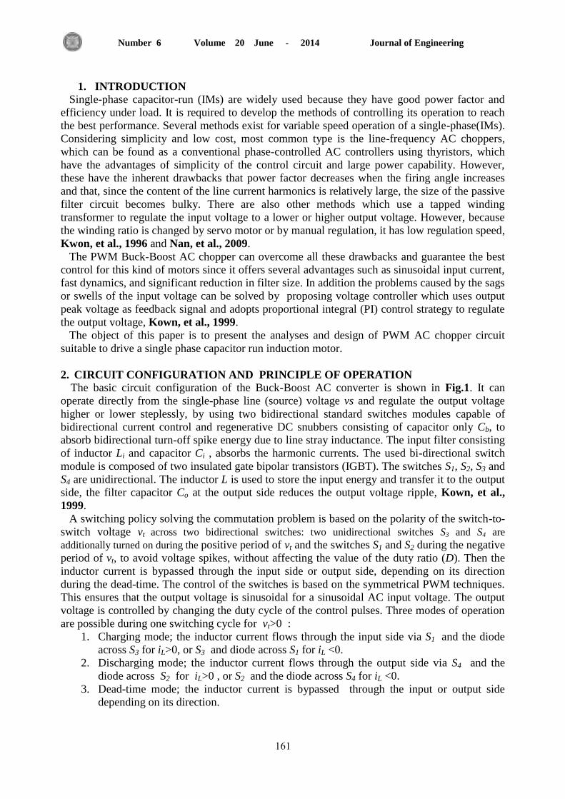
Journal of Engineering Volume 20 June - 2014 Number 6
060
1. INTRODUCTION Single-phase capacitor-run (IMs) are widely used because they have good power factor and
efficiency under load. It is required to develop the methods of controlling its operation to reach
the best performance. Several methods exist for variable speed operation of a single-phase(IMs).
Considering simplicity and low cost, most common type is the line-frequency AC choppers,
which can be found as a conventional phase-controlled AC controllers using thyristors, which
have the advantages of simplicity of the control circuit and large power capability. However,
these have the inherent drawbacks that power factor decreases when the firing angle increases
and that, since the content of the line current harmonics is relatively large, the size of the passive
filter circuit becomes bulky. There are also other methods which use a tapped winding
transformer to regulate the input voltage to a lower or higher output voltage. However, because
the winding ratio is changed by servo motor or by manual regulation, it has low regulation speed,
Kwon, et al., 1996 and Nan, et al., 2009.
The PWM Buck-Boost AC chopper can overcome all these drawbacks and guarantee the best
control for this kind of motors since it offers several advantages such as sinusoidal input current,
fast dynamics, and significant reduction in filter size. In addition the problems caused by the sags
or swells of the input voltage can be solved by proposing voltage controller which uses output
peak voltage as feedback signal and adopts proportional integral (PI) control strategy to regulate
the output voltage, Kown, et al., 1999.
The object of this paper is to present the analyses and design of PWM AC chopper circuit
suitable to drive a single phase capacitor run induction motor.
2. CIRCUIT CONFIGURATION AND PRINCIPLE OF OPERATION
The basic circuit configuration of the Buck-Boost AC converter is shown in Fig.1. It can
operate directly from the single-phase line (source) voltage vs and regulate the output voltage
higher or lower steplessly, by using two bidirectional standard switches modules capable of
bidirectional current control and regenerative DC snubbers consisting of capacitor only Cb, to
absorb bidirectional turn-off spike energy due to line stray inductance. The input filter consisting
of inductor Li and capacitor Ci , absorbs the harmonic currents. The used bi-directional switch
module is composed of two insulated gate bipolar transistors (IGBT). The switches S1, S2, S3 and
S4 are unidirectional. The inductor L is used to store the input energy and transfer it to the output
side, the filter capacitor Co at the output side reduces the output voltage ripple, Kown, et al.,
1999.
A switching policy solving the commutation problem is based on the polarity of the switch-to-
switch voltage vt across two bidirectional switches: two unidirectional switches S3 and S4 are
additionally turned on during the positive period of vt and the switches S1 and S2 during the negative
period of vt, to avoid voltage spikes, without affecting the value of the duty ratio (D). Then the
inductor current is bypassed through the input side or output side, depending on its direction
during the dead-time. The control of the switches is based on the symmetrical PWM techniques.
This ensures that the output voltage is sinusoidal for a sinusoidal AC input voltage. The output
voltage is controlled by changing the duty cycle of the control pulses. Three modes of operation
are possible during one switching cycle for vt>0 :
1. Charging mode; the inductor current flows through the input side via S1 and the diode
across S3 for iL>0, or S3 and diode across S1 for iL <0.
2. Discharging mode; the inductor current flows through the output side via S4 and the
diode across S2 for iL>0 , or S2 and the diode across S4 for iL <0.
3. Dead-time mode; the inductor current is bypassed through the input or output side
depending on its direction.

Journal of Engineering Volume 20 June - 2014 Number 6
062
Fig. 2a-c show the inductor current and voltage waveforms for vt > 0 during one switching
cycle. The inductor voltage vL is vi during the charging mode and vo during the discharging mode
as shown in Fig. 2b and c. Because the switches S3 and S4 are turned on for vt > 0, the inductor
voltage vL is vo or vi, according to the direction of iL during the dead-time mode, Kim, et al.,
2011.
3. ANALYSIS
To facilitate the analytical procedure in order to obtain an equivalent circuit for the buck-boost
AC chopper, all components are assumed ideal and the switching frequency fs is much greater
than the line frequency f, so that during a switching period, the input and output voltage can be
cosidered constant. The average inductor voltage during one switching period Ts = 1/fs is given
by, Kown, et al., 1999:
)()1()()( tvDtDvtv oiL (1)
Where vi(t) and vo(t) are the average AC input voltage and output voltage, respectively, during
the switching period, and D is the duty ratio. The inductor voltage is given by:
dt
tdiLtv L
L )( (2)
Where iL(t) is the average inductor current during the switching period. If charging the inductor
by the input current will take a time equals to (Ton), then discharging the inductor current to the
load can be represented by the following equation:
)(1)( tiDti Lo (3)
Where:
)()( tDiti Li (4)
Where io(t) and ii(t) are the average output and input current respectively. From Eqs. (1) and (2),
the following equation is obtained:
)(1)( tvD
dt
tdiLtDv o
Li
(5)
Substituting Eq. (3) in Eq. (5), yields:
)(
1)(
12
tvdt
tdi
D
Ltv
D
Do
oi
(6)
Eq. (6) represents the steady-state equivalent circuit for the chopper type voltage regulator. The
equivalent circuit is shown in Fig.3. At steady-state motor impedance including (Ro and Xo)

Journal of Engineering Volume 20 June - 2014 Number 6
061
varies according to the load applied to the motor which is 175W single phase capacitor-run
induction motor. From the equivalent circuit shown in Fig.3, the transfer function of the output
voltage Vo(s) with respect to the input voltage Vi(s) is obtained as, appendix A, Kamel, 2013:
oooooo
oo
i
o
RDLDLsRLCsCLLs
sLRDD
sv
sv2223 1]1[
1
(7)
From Eq. (3) and Eq. (7), Eq. (8) is obtained
oooooo
oooo
i
L
RDLDLsRLCsCLLs
RsCCLsD
sV
sI2223
2
1]1[
]1[
(8)
The source current Is(s) and source voltage Vs(s) are obtained as
sIsDIsI ciLs
i
oooooo
ooooi sC
RDLDLsRLCsCLLs
RsCCLsDsV
2223
22
1]1[
]1[ (9)
svsI)(v is is sLs
1
1]1[
]1[ 2
2223
22
ii
oooooo
ooooii CLs
RDLDLsRLCsCLLs
RsCCLsDsLsV
(10)
From Eq. (9) and Eq. (10), the following relation is obtained for simplicity:
01
2
2
3
3
4
4
01
2
2
3
3
4
4
5
5
bsbsbsbsb
asasasasasa
sIs
sVs
(11)
Where: a5=CiLiLLoCo, a4=LLiCoCiRo, a3=[D2LiLoCo+ LiCi[L+(1-D)2Lo+LLoCo],
a2=[D2LiCoRo+CiLi(1-D)
2 Ro+LCoRo], a1=[LiD
2+L+(1-D)
2Lo], ao=(1-D)
2Ro, b4= CiCoLLo,
b3=LCoCiRo, b2=[D2LoCo+Ci[L+(1-D)
2Lo]], b1=[D
2CoRo+(1-D)
2CiRo], bo= D
2
Under an appropriate selection of the parameters L, Li, Co and Ci satisfying
a5 a4 a3 a2 b4 b3 b2 b1 0, Eq. (10) can be approximated as follows:
2
222
)1(])1([
sIs
sVs
D
RDLDLDLs ooi
[ ]
(12)

Journal of Engineering Volume 20 June - 2014 Number 6
061
From Eq. (12), the angle of the power factor is given by
o
oi
RD
LDLDL2
22
)1(
])1([tanθ 1
[ ]
(13)
Where is the angular frequency of the source voltage.
Derivation of equations: (7, 8, 9, 10 and 12) are shown in appendix A, Kamel, 2013.
4. DESIGN OF INPUT AND OUTPUT FILTERS AND VOLTAGE CONTROLLER
For fast dynamic response the voltage controller, which uses the output peak-voltage as the
feedback signal, is designed to keep the stability of the output voltage in case of input voltage
fluctuation. The peak-voltage detector system is shown in Fig.4. Where vo is the rms voltage
across the load terminals, vod is the sensed output of the proposed detector, kd is the detection
gain and Vo is the peak value of the output voltage. A fast detection technique is composed of a
phase shifter, two multipliers, and an adder. The detection technique utilizes the simple
trigonometric principle as follows, Kown, et al., 1999 :
(14)
The sensed output vod is:
(15)
When the disturbed input vi , is applied to the system, the sensed output vod (disturbed by the
disturbance input) needs to be regulated to a desired constant reference Vr with no steady-state
error where Vr is kd2Vor
2 and Vor is the peak value of the desired output voltage. A good response
is obtained by using a traditional PI controller. The integral part of the designed controller makes
the steady-state output voltage error zero. The controller output is duty ratio D, Nan, et al., 2009:
∫ (16)
Where kp and ki are proper proportional and integral gains respectively. Δv is the controller input:
Δv = Vr − vod (17)
A filter must be added at the power input of a switching converter for improving power
quality and interface issues. Low pass input LC filter needs to be damped at the corner frequency
fc to prevent the gain of the filter to go to infinity otherwise, this rise would cause extreme
current peaks which would make the system worse than if it was without filter. Taking into
account only the dominant harmonic, the input current of the converter is represented with good
approximation by, Barbi, et al., 1991:
(18)
Where Iip is the peak value of the input current, thus,

Journal of Engineering Volume 20 June - 2014 Number 6
061
(19)
The role of the input filter is to prevent the harmonic current ih from circulating through inductor
Li . According to the harmonic equivalent circuit shown in Fig.5:
(20)
According to the usual specification, the total harmonic distortion (THD) of the input current ii
is ≤ 5%. Then reducing the value of iLhp (which is the maximum harmonic current circulating
through inductor Li ) to 3% of input current, the THD ≤ 5% is ensured, Barbi, et al., 1991
=> , where
then using Eq. (20):
(21)
rad/s, where
fs=25KHZ, Let Li=0.5mH , then
F. A value of 3μF is chosen.
A damped filter made with a resistor Rd in series with a capacitor Cd as shown in Fig.6, all
connected in parallel with the filter’s capacitor Ci. The purpose of resistor Rd is to reduce the
output peak impedance of the filter at the cutoff frequency. The choice of Cd ,that leads to the
minimum peak output impedance, for a given value of Rd can be expressed as following:
For Cd =20µF, then
=> n=6.7 , the optimum damping resistance value Rd is equal to, Erickson, 1999:
√
√
≈ 6Ω (22)
The filter high-frequency attenuation is not affected by the choice of Cd and the high-frequency
asymptote is identical to that of the original undamped filter, Erickson, 1999. The energy
storage inductor L is used to store the energy from the source during the active mode of the
chopper operation, then transfer it to the load during the discharging mode. During one switching
period Ts, inductor must be satisfied such that, Li, et al., 2011:
(23)

Journal of Engineering Volume 20 June - 2014 Number 6
066
With maximum value of duty ratio evaluated from, Li, et al., 2011:
(
) (24)
= 0.578
And for typical values of output current = 1.4A, Kamel, 2013, η (convertor efficiency)=90%,
kc (ripple coefficient of inductor current) ≤0.5, Li, et al., 2011. The boundary Lmin =1mH, for L
≥ Lmin., the convertor operates in continuos conduction mode(CCM). A value of 1mH is chosen.
Output filter capacitor is used to reduce the output voltage ripple and harmonics. During one Ts ,
to limit the output voltage ripple ,output filter capacitor Co must satisfy the following, Li, et al.,
2011:
With kv (ripple coefficient of output voltage) ≤0.1, Li, et al., 2011, the boundary Comin equals to
1.43µF, for Co more than or equal to Comin (Co ≥ Comin); A value of 10 µF is chosen in the
simulation to ensure output voltage without harmonics.
5. SIMULATION RESULTS
To show the feasibility of the proposed analysis method and control strategy, the simulation
model of the proposed voltage regulator is implemented using Matlab/Simulink software. The
induction motor whose its specifications shown in Table 1 and its measured parameters listed in
Table 2 are used in the simulation, Kamel, 2013. THD values for current input to the chopper
and motor input current and voltage are listed in Table 3 (the values are obtained by using
Matlab/Simulink).
5.1 Results for Sudden Change of Supply Voltage from (220V rms) Value to (160V rms)
Value
At normal operation the supply produces rms voltage equals to the rated voltage (220V); if
suddenly a disturbance occurred in the system leads to drop the voltage to (160V) rms value,
then the voltage controller will detect it and the AC chopper will regulate the dropped voltage to
be the same as the rated voltage needed by the motor.
5.1.1 No-load condition
Fig. 7 shows the simulated waveform of the supply voltage and load voltage at no-load and at
source main frequency of 50HZ. In this figure it is shown that after (0.5sec), the load voltage
dropped then increased gradually within (60msec) to reach its rated (rms value =220V) with low
THD equals to (0.35%) even if the supply continues on the low level (160V). Fig. 8 shows the
simulated waveform of the supply current which has rms value equals to (1.76A), with (THD =
4.09%). Fig. 9 shows the simulated waveform of the motor input current, the disturbance
occured at (0.5sec), current decreased temporarily (since voltage across load terminals dropped
temporarily) then gradually increased to reach (rms value = 0.56A). Motor speed is shown in
Fig. 10, at no-load motor runs at (1500rpm), after the disturbance occurred, the motor speed
dropped temporarily corresponding to the drop in load voltage, then the motor returns to run at
no-load speed.
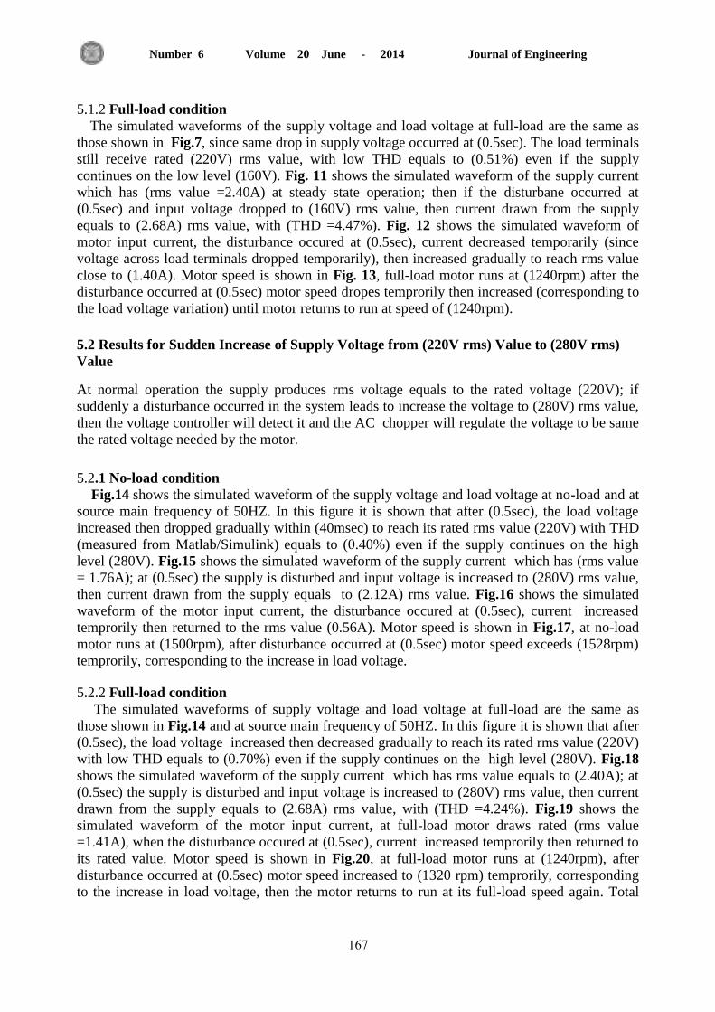
Journal of Engineering Volume 20 June - 2014 Number 6
061
5.1.2 Full-load condition
The simulated waveforms of the supply voltage and load voltage at full-load are the same as
those shown in Fig.7, since same drop in supply voltage occurred at (0.5sec). The load terminals
still receive rated (220V) rms value, with low THD equals to (0.51%) even if the supply
continues on the low level (160V). Fig. 11 shows the simulated waveform of the supply current
which has (rms value =2.40A) at steady state operation; then if the disturbane occurred at
(0.5sec) and input voltage dropped to (160V) rms value, then current drawn from the supply
equals to (2.68A) rms value, with (THD =4.47%). Fig. 12 shows the simulated waveform of
motor input current, the disturbance occured at (0.5sec), current decreased temporarily (since
voltage across load terminals dropped temporarily), then increased gradually to reach rms value
close to (1.40A). Motor speed is shown in Fig. 13, full-load motor runs at (1240rpm) after the
disturbance occurred at (0.5sec) motor speed dropes temprorily then increased (corresponding to
the load voltage variation) until motor returns to run at speed of (1240rpm).
5.2 Results for Sudden Increase of Supply Voltage from (220V rms) Value to (280V rms)
Value
At normal operation the supply produces rms voltage equals to the rated voltage (220V); if
suddenly a disturbance occurred in the system leads to increase the voltage to (280V) rms value,
then the voltage controller will detect it and the AC chopper will regulate the voltage to be same
the rated voltage needed by the motor.
5.2.1 No-load condition
Fig.14 shows the simulated waveform of the supply voltage and load voltage at no-load and at
source main frequency of 50HZ. In this figure it is shown that after (0.5sec), the load voltage
increased then dropped gradually within (40msec) to reach its rated rms value (220V) with THD
(measured from Matlab/Simulink) equals to (0.40%) even if the supply continues on the high
level (280V). Fig.15 shows the simulated waveform of the supply current which has (rms value
= 1.76A); at (0.5sec) the supply is disturbed and input voltage is increased to (280V) rms value,
then current drawn from the supply equals to (2.12A) rms value. Fig.16 shows the simulated
waveform of the motor input current, the disturbance occured at (0.5sec), current increased
temprorily then returned to the rms value (0.56A). Motor speed is shown in Fig.17, at no-load
motor runs at (1500rpm), after disturbance occurred at (0.5sec) motor speed exceeds (1528rpm)
temprorily, corresponding to the increase in load voltage.
5.2.2 Full-load condition
The simulated waveforms of supply voltage and load voltage at full-load are the same as
those shown in Fig.14 and at source main frequency of 50HZ. In this figure it is shown that after
(0.5sec), the load voltage increased then decreased gradually to reach its rated rms value (220V)
with low THD equals to (0.70%) even if the supply continues on the high level (280V). Fig.18
shows the simulated waveform of the supply current which has rms value equals to (2.40A); at
(0.5sec) the supply is disturbed and input voltage is increased to (280V) rms value, then current
drawn from the supply equals to (2.68A) rms value, with (THD =4.24%). Fig.19 shows the
simulated waveform of the motor input current, at full-load motor draws rated (rms value
=1.41A), when the disturbance occured at (0.5sec), current increased temprorily then returned to
its rated value. Motor speed is shown in Fig.20, at full-load motor runs at (1240rpm), after
disturbance occurred at (0.5sec) motor speed increased to (1320 rpm) temprorily, corresponding
to the increase in load voltage, then the motor returns to run at its full-load speed again. Total

Journal of Engineering Volume 20 June - 2014 Number 6
061
harmonic distortion (THD) for input current, load current and voltage across the load terminals
after disturbing input voltage at (0.5sec) are shown in Table 3 (The values of (THD) are
obtained by using Matlab/Simulink software); it is seen that the design of input filter ensures that
(THDi > 5%), also load current and load voltage has a low value of (THD) since the output filter
is well designed. Table 4 illustrates how the input power (W) that is drawn from the source,
varies with the line power factor which is measured by using Matlab/Simulink, depending on the
equation: p.f =P/(P2+Q
2)1/2
, where P and Q are active and reactive input powers respectively and
p.f is the input power factor.
6. CONCLUSION
The analysis of Buck-Boost AC chopper circuit, that can regulate output voltage higher or
lower steplessly is presented. The input current is sinusoidal waveform with low harmonic
components. The output voltage control system is designed using PI control method and the
peak-voltage detector. The simulation results show that the voltage controller has a good
dynamic performance when input voltage swells or sags occur, since the output voltage returns
to its normal value of (220V) rms value after no more than three cycles (60msec). The results
show low total harmonic distortion factor for input current, load current and load voltage. The
AC chopper achieves an acceptable line power factor at full load with low input voltage, since
(D) will be increased, according to Eq. (13), the motor needs a power (175W) to run at full load,
but the power drawn from the source is higher, the difference represents the losses since in the
construction of the motor the resistances of its windings are very high, appendix B, Kamel,
2013.
REFERENCES
Barbi, Fagundes, J. C., and Kassick, E. V., 1991, A Compact AC/AC Voltage Regulator Based
on An AC/AC High Frequency Flyback Converter, IEEE Power Electronics Specialists
Conference 22nd
Annual, pp. 846-852.
Erickson, R.W., 1999, Optimal Single Resistor Damping of Input Filters, IEEE Applied Power
Electronics Conference and Exposition, 14th Annual , Vol.2, pp.1073-1079.
Kamel, S. W., 2013, Analysis of Buck-Boost AC Chopper Fed Capacitor Run Induction Motor,
A thesis submitted in fulfillment of requirements for award of the Master of engineering,
Electrical Department, Engineering College, University of Baghdad.
Kim, J.H., Min, B. D., Kwon, B. H., and Won, S. C., 2011, A PWM Buck-Boost AC Chopper
Solving the Commutation Problem, IEEE Trans. on Indust. Electronics, Vol.45, No. 5.
Kown, B. H., Youm, J. H., and Choi, J. H., 1999, Automatic Votage Regulator with Fast
Dynamic Speed, IEEE Proc.-Elect., Power Appl.Vol. 146. No.2.
Kwon, B.-H., Min, B.-D., and Kim, J.-H., 1996, Novel Topologies of AC Choppers, IEEE proc.
–Elect, Power Appl, Vol 143, No. 4.
Li, L., Yang, J., and Zhong, Q., 2011, Novel Family of Single-Stage Three-Level AC Choppers,
IEEE Trans. on Power Electronics, Vol.26, No. 2.

Journal of Engineering Volume 20 June - 2014 Number 6
061
Nan, J., Hou-jun, T., Wei, L. and Peng-sheng, Y., 2009, Analysis and Control of Buck-Boost
Chopper Type AC Voltage Regulator, IEEE Power Electronics and Motion Control, 6th
International Conference, pp.1019-1023.
NOMENCLATURE
Cb = snubber capacitor, μF.
Cd = damping capacitor, μF.
Ci = input capacitor, μF.
Co = output capacitor, μF.
D = duty ratio.
f = main frequency, Hz.
fc = corner frequency, Hz.
fs = switching frequency, Hz.
i1 = output capacitor current, A.
i2 = load current, A.
iCi = input capacitor current, A.
ih = harmonic current, A.
Ihp= peak harmonic current, A.
ii(t) = average input current during the switching period, A.
Iip = peak converter input current, A.
iL(t)= average inductor current during the switching period, A.
ILhp= peak harmonic current in input inductance, A.
io(t) = average output current during the switching period, A.
is = source current, A.
kc = ripple coefficient of inductor current.
kd = detection gain of the output voltage.
kp , ki = proportional and integral gains respectively.
kv = ripple coefficient of output voltage.
L = energy storage inductor, mH.
Li = input inductor, mH.
Rd= damping resistance, Ω.
Ro= resistance of the load, Ω.
S1= first unidirectional switch.
S2= second unidirectional switch.
S3= third unidirectional switch.
S4= forth unidirectional switch.
Ts = one switching period, s.
vi(t)= average input voltage, V.
vL(t)= average inductor voltage, V.
vo(t)= average output voltage, V.
vod = detected output peak-voltag, V.
vr = reference voltage, V.
vs = source voltage, V.
vt = switch-to-switch voltage across two bidirectional switches, V.
Xo =inductance of the load, Ω.
Zo= output impedance, Ω.
η= conversion efficiency.
θ= input phase angle.

Journal of Engineering Volume 20 June - 2014 Number 6
011
θo= output phase angle.
ξ= damping factor.
= a ngular frequency of the source voltage, rad/s.
s= angular switching frequency, rad/s.
9 FIGURES AND TABLES
Figure1. Buck-boost AC chopper circuit configuration.
Figure 2. a.Gate signals, b. Inductor current and voltage waveforms
for vt>0, iL>0 during one switching cycle,c. iL and vL for iL<0.
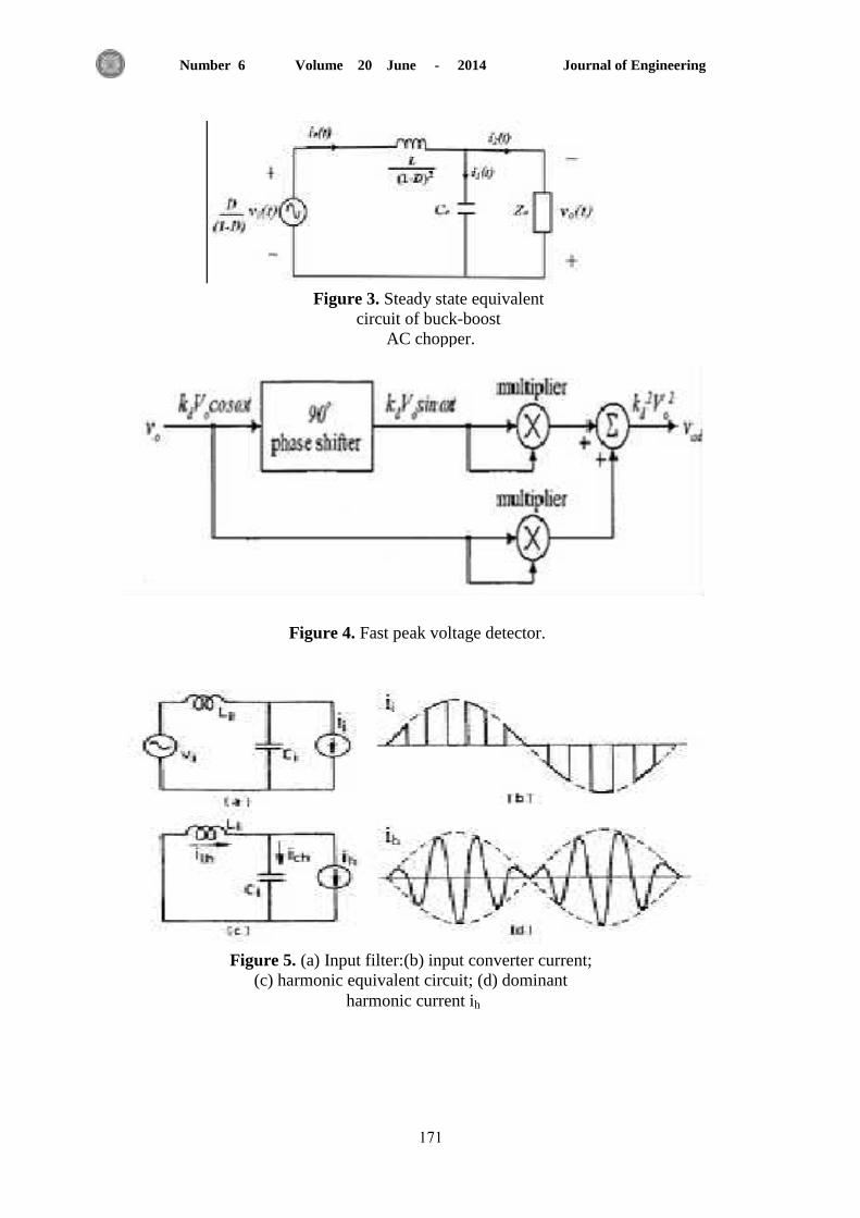
Journal of Engineering Volume 20 June - 2014 Number 6
010
Figure 3. Steady state equivalent
circuit of buck-boost
AC chopper.
Figure 4. Fast peak voltage detector.
Figure 5. (a) Input filter:(b) input converter current;
(c) harmonic equivalent circuit; (d) dominant
harmonic current ih
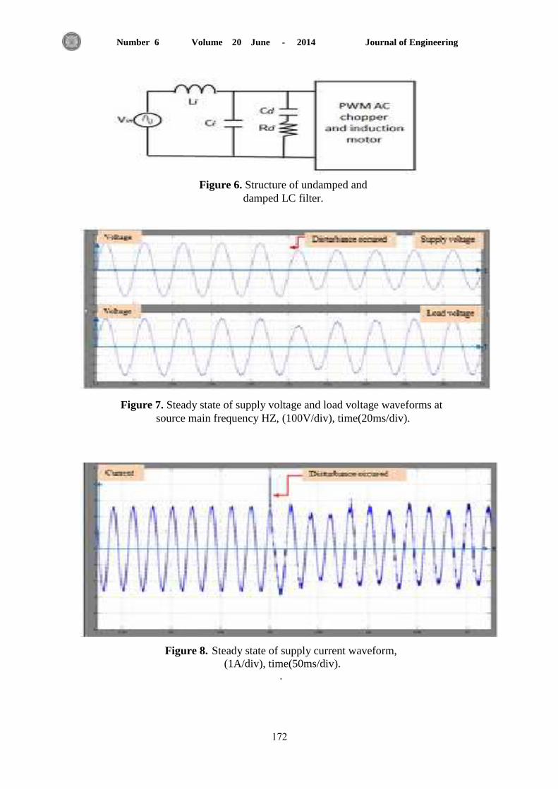
Journal of Engineering Volume 20 June - 2014 Number 6
012
Figure 6. Structure of undamped and
damped LC filter.
Figure 7. Steady state of supply voltage and load voltage waveforms at
source main frequency HZ, (100V/div), time(20ms/div).
Figure 8. Steady state of supply current waveform,
(1A/div), time(50ms/div). .

Journal of Engineering Volume 20 June - 2014 Number 6
011
Figure 9. Steady state of motor input current waveform,
(500mA/div), time(50ms/div).
Figure 10. Steady state motor speed at source main frequency 50HZ,
(20rad/s/div), time(s).
Figure 11. Steady state of supply current waveform,
(2A/div), time(50ms/div).

Journal of Engineering Volume 20 June - 2014 Number 6
011
Figure 12. Steady state of motor input current waveform,
(500mA/div), time(50ms/div).
Figure 13. Steady state motor speed at source main frequency 50HZ,
(20rad/s/div), time(s).
Figure 14. Steady state of supply voltage and load voltage waveforms at
source main frequency 50HZ, (100V/div), time(100ms/div).

Journal of Engineering Volume 20 June - 2014 Number 6
011
Figure 15. Steady state of supply current waveform,
(1A/div), time(100ms/div).
Figure 16. Steady state of motor input current waveform,
(500mA/div), time(50ms/div).
Figure 17. Steady state motor speed at source main frequency 50HZ,
(20rad/sec/div), time(s).

Journal of Engineering Volume 20 June - 2014 Number 6
016
Figure 18. Steady state of supply current waveform,
(1A/div), time(50ms/div).
Figure 19. Steady state of motor input current waveform,
(1A/div), time(50ms/div).
Figure 20. Steady state motor speed at source main frequency 50HZ,
(20rad/sec/div), time(s).

Journal of Engineering Volume 20 June - 2014 Number 6
011
Induction motor
Parameter Value
Rated rms voltage 220 V
Rated frequency 50 HZ
Rated rms current 1.47 A
Number of poles 4
Capacitor 8 µ F ± 7%
Rated output 175 W
Rated speed 1140±40% rpm
Parameter value
Main winding stator resistance
43Ω
Main winding stator leakage
reactance 34.05 Ω
Main winding rotor resistance 32.76 Ω
Main winding rotor leakage
reactance 34.05 Ω
Main winding mutual
reactance 466.60 Ω
Auxiliary winding stator
resistance 23Ω
Auxiliary winding stator
leakage reactance 40 Ω
turn ratio (aux/main ) 1.1
Moment of inertia(J) 0.767x10^-3
Kg.m2
Friction coefficient 0.118x10 ^-3
N.m.s/rad
Table 1. Name-plate data of the single phase
capacitor run induction motor.
Table 2. Motor parameters.

Journal of Engineering Volume 20 June - 2014 Number 6
011
Voltage variation Load condition THDi THDiL THDvo
Rated rms input
voltage dropped
to(160V)
No-load 4.09% 3.80% 0.60%
Half-full load 4.53% 1.97% 0.59%
Full-load 4.47% 1.52% 0.51%
Rated rms input
voltage increased
to(280V)
No-load 3.29% 3.31% 0.40%
Half-full load 3.44% 2.25% 0.46%
Full-load 4.24% 1.32% 0.70%
Input
voltage
(V)
Source
Current
(A)
Load
applied on
the motor
(N.m)
Input
power
factor
Input
capacity
(VA)
Input
power
(W)
(160V)
1.76 0 0.355 281.6 99.9
2.68 1.3 0.810 428.8 347.3
(220V)
1.76 0 0.250 387.2 96.8
2.47 1.3 0.650 543.4 353.2
(280V)
2.12 0 0.170 593.6 100.9
2.47 1.3 0.500 691.6 345.8
Table 3. Total harmonic distortion; for input current, load current and voltage
across the load terminals when input voltage varied at (0.5sec).
Table 4. Input power (W) values according to line power factor variation at
different supply voltage.

Journal of Engineering Volume 20 June - 2014 Number 6
179
Numerical Study of Optimum Configuration of Unconventional Airfoil with
Steps and Rotating Cylinder for Best Aerodynamics Performance
Dr. Najdat N. Abdulla Ahmed J. Hamoud
Professor M.sc.
College of Engineering-University of Baghdad College of Engineering-University of Baghdad
[email protected] [email protected]
ABSTRACT
Numerical study of separation control on symmetrical airfoil, four digits (NACA
0012) by using rotating cylinder with double steps on its upper surface based on the computation of
Reynolds-average Navier- Stokes equations was carried out to find the optimum configuration of
unconventional airfoil for best aerodynamics performance. A model based on collocated Finite
Volume Method was developed to solve the governing equations on a body-fitted coordinate
system. A revised (k-w) model was proposed as a known turbulence model. This model was
adapted to simulate the control effects of rotating cylinder. Numerical solutions were performed for
flow around unconventional airfoil with cylinder to main stream velocities ratio in the range of 1 to
4 and for various positions of the steps on the airfoil from the leading edge, 0.1c, 0.2c, 0.3c, 0.4c,
0.5c for the first step and 0.5c, 0.6c, 0.7c, 0.8c for the second step with constant step depth and
length of 0.03c and 0.125c respectively. Reynolds number of 700,000 which was based on the cord
length (c), with angle of attacks 0, 5, 8, 10, 12, 15 degrees was considered for the assessment of the
unconventional airfoil performance. The numerical investigation showed that the optimum
configuration for the unconventional airfoil was found to be at velocities ratio (U/U∞=4) with the
steps positions at 0.5c and 0.8c for best airfoil performance.
Keywords: unconventional airfoil, airfoil with rotating cylinder, airfoil with upper steps.
هوائألفضل اداء دنامك لجناح غر تقلدي حوي على عتبات واسطوانة دوارة للشكل االمثل دراسة عددة
احمد جمل حمود نجدت نشأت عبدهللا د. ماجستر استاذ
جامعة بغداد -كلة الهندسة جامعة بغداد -كلة الهندسة
الخالصة
ان الهواء من على سطح جناح متناظر نوع للسطرة على انفصال جر عددةتضمن العمل دراسة (NACA 0012( باستخدام
نافر -متوسط رنولدباستخدام معادلة ي للجناح, وهذا التحلل تماسطوانة دوارة ف مقدمة الجناح واضافة عتبات اثنن على السطح العلو, وقد تم المحددة لحل حجومطرقة الهذا المودل الراض على اعتمد ستوك( وذلك الجاد افضل اداء ارودنامك للجناح بعد االضافات.
السرعات نسبةدوارة ب اسطوانة مع تقلدةال غر الجناح حول للتدفق العددي الحل أجري .جران االضطرابلل استخدام مودل راض عددوقد كان األمامة الحافة منبمسافة مقاسة الجناح علىعتبات ال اماكن اختالف ومعاضعاف سرعة التار الهوائ الرئس 4الى 1من
.تقلدة غر حالجنا األداء لتقم درجة 15 ،11 ،17 ،8 ،5 ،7 الهجمات من زاوة مع 077.777 من رنولدز

Journal of Engineering Volume 20 June - 2014 Number 6
180
1. INTRODUCTION
In modern civil transport aircraft, the main objectives to be achieved are the needs of cruise
conditions (low drag) with a particular attention on the economic, as well as aerodynamic efficiency
because most of the flight time is spent during this phase of flight at transonic conditions. Hence,
the shape of the wing must be able to minimize the strength of any shock waves present in order to
reduce the wave drag. In addition, the wing must be able to satisfy the necessary requirements of
take-off and landing. Therefore, complementary high-lift systems are usually employed by combat
aircraft, not only for short take-off and landing, but also to enhance high-speed maneuverability by
delaying the onset of high-speed stall. High-lift system mainly consists of mobile mechanical device
capable of separating some parts of the wing and repositioning them in a suitable configuration in
order to increase the chamber and effective area of the wing. The result of these arrangements is a
new configuration, which allows a significant improvement in lifting capabilities compared to the
clean wing of the cruise configuration. The first practical application of the moving surface for the
boundary layer control was demonstrated by, Favre, 1938. He studied an airfoil with an upper
surface formed by a belt moving over two rollers. The separation was delayed until the angle of
attack reached to 55 degree, where the maximum lift coefficient of 3.5 was realized. Cichy, et al.,
1972, studied the application of rotating cylinder to improve ship maneuverability. Extension force
measurements and flow visualization experiments were conducted using a large circulating water
channel. Three different configurations of rudder were used with the rotating cylinder; (1) in
insulation, (2) the leading-edge of the rudder, and (3) combined with a flap-rudder where the
cylinder being at the leading-edge of the flap. From the overall consideration of hydrodynamic
performance and mechanical complexity, configuration number (2) was preferred as far as power
consumption concerned. Buckholtz, 1986, observed the irregular shape of many insect wings as
well as other studies indicating a higher lift on these wings. A flow visualization scheme was used
to observe and photograph stream lines around two different wing sections. One of these, a sheet
metal model with geometry matching that of a butterfly wing, was studied at a Reynolds number of
1500 and 80 based on corrugation depth. Freymuth,et al, 1989, worked on the airfoil with rotating
cylinder at the nose to demonstrate concept of dynamic separation without dynamic stall. The airfoil
was tested in the wind tunnel with uniform velocity of 61 cm/s and cylinder rotating speed of 3000
r.p.m. at a Re=4300 based on the chord length. They found that for a pitch angle of 20o a speed ratio
was 2.5, for 40o the ratio was 4.2, and at 90
o it was 12. An increase in speed ratio beyond the
minimum had no detrimental effect on stall control but resulted in a wall jet passing over the suction
side of the airfoil which continued as a jet behind the trailing edge. These results were inferred from
flow visualization and confirmed by speed profiles obtained with a hot-wire anemometer, after the
final pitch position of the airfoil had been reached. Al- Tornachi, and Abu- Tabikh, 1998,
developed a numerical method to analyze steady incompressible flow around airfoils with turbulent
separation. The model used was a direct viscous- inviscid interaction scheme based on a vortex
panel method. The overall method was relatively simple and allowed for predicting the complete
wing characteristics. Some example calculations were discussed, and good agreement between
calculations and experiment was obtained. Al-Garni, et al., 2000, worked on the experimental
investigation of two –dimensional NACA 0024 airfoil equipped with a leading-edge rotating
cylinder. The airfoil was stated for different angles, and they found that the leading-edge rotating
cylinder increases the lift coefficient of a NACA 0024 airfoil from 0.85 at Uc/U=0 to 1.63 at
Uc/U=4 and delay the stall angle of attack by about 160%. In the same year, Yeung, 2000, studied

Journal of Engineering Volume 20 June - 2014 Number 6
181
the flow visualization on a corrugated airfoil. He confirmed that the trapped vortices leaded to a
modification of the effective wing shape and an increase in lift. He also, found that the leading-edge
rotating cylinder effectively extend the lift curve of an airfoil without substantially affecting its slop.
Sahu, and Patnaik, 2010, investigated the flow past NACA 0012 airfoil. The simulations were
performed for different angles of attack varying from 0o to 20
o in sub- critical Reynolds numbers
range. The results observed that, stall occurred at ɑ=12o and Re=46400.Also, the stall angle was
delayed by using the simple momentum injection technique with the help of one rotating element as
an actuator disc on the leading edge of airfoil. Lukas, et al., 2011, studied the boundary layer
separation, both stall and separation bubbles, related to the low-Reynolds number transition
mechanism. Airfoil of three czech-designed sailplanes and their wing-fuselage interaction were
subjected to study. Effect of passive flow control device-vortex generators was surveyed and
counter- rotating vortex generators was applied. Separation suppression was reached and
consequent drag coefficient reduction of test aircrafts was measured in flight. All above studies
were neither considered the combine effects of leading edge rotating cylinder and the steps on the
upper side of airfoil nor high Reynolds numbers flow.
The present work investigate the combine effect of the rotating cylinder of diameter 0.1c in
leading edge and double steps at different locations with constant depths and length on the upper
side of airfoil. Symmetrical airfoil four digits, (NACA 0012) with Reynolds number of 700000
were considered in this work. Upon the numerical results of all above considered cases, an optimum
configuration of airfoil which is represented by lengths, depths and positions of each step in
addition to the cylinder to mainstream velocities ratio were obtained for the best performance
enhancement of unconventional airfoil.
2. MATHEMATICAL FORMULATION
2.1 Governing Partial Differential Equations
In the present work, the working fluid is air and flow was considered to be steady, two
dimensional mean flows, fully turbulent, incompressible, and Newtonian fluid.
The governing equations were derived in Cartesian coordinate systems. Finite volume methods
for solving differential equations require continuous physical space to be discretized into a uniform
computational space. However, the applications of the boundary conditions require that the
boundaries of the physical space fall on coordinate lines of the coordinate system.
In order to analyze the flow field around the airfoil with rotating cylinder and two steps, solution of
two dimensional Navier-Stokes equations is required, due to the complexity of flow around airfoil
configurations and the dominancy of viscosity effects.
The governing equations for the mean velocity and pressure are the mass and momentum equations,
these are analyzed the averaged Navier- Stokes equations. A two- equation turbulence model (k-ω)
is used for the system of the momentum equations.
2.2 Reynolds-averaged Navier- Stokes Equations
The basic governing fluid flow equations for, incompressible flows will be summarized. The
derivation of these equations, details regarding the constitutive relations used and the various
turbulence modeling assumptions employed can be found in several references, White, 1991,and
Ferziger and Peric, 1999.

Journal of Engineering Volume 20 June - 2014 Number 6
182
Employing indicial notation, the instantaneous form of continuity and momentum equations in
Cartesian coordinates can be written as follows:
( )
(1)
( )
(2)
Where is position vector, is viscous stress tensor. The constitutive relation between stress and
strain rate for a Newtonian fluid is used to relate the components of the stress tensor to velocity
gradients:
(
)
(3)
Where represents the molecular viscosity and is the Kronecker delta. The conservation
equations above hold exactly for laminar flows. For turbulent flows, in the context of RANS
methods, ensemble averaging will be resorted. The time- averaged form of the above equations for
turbulent flows is obtained by mass- averaging. The various flow properties are decomposed into
mean and fluctuating components, as follows:
(4)
(5)
(6)
Note that Favre-averaging is used for and (bar and prime denote a Favre- averaging mean
quantity and the fluctuation above this mean, respectively). Reynolds- averaging is used for P (bar
and prime denote a Reynolds- Averaged mean quantity and the fluctuation above this mean,
respectively). After mass- averaging, the mean- flow governing equations become:
(7)
( )
(
)
(8)
The double correlation between and itself, which appears in the term on the right hand side of
equation , is the kinetic energy per unit volume (k) of the turbulent velocity fluctuations and can be
defined as:
(9)
The term
is called the Reynolds-stress tensor and can be shown by:
(10)
Or
(11)

Journal of Engineering Volume 20 June - 2014 Number 6
183
(
)
(12)
Two major approaches are currently used to model these terms, namely:
(a) Eddy Viscosity Models (EVM)
(b) Reynolds- Stress Models (RSM)
The EVM employ Boussineq’s eddy hypothesis, which relates the Reynolds stresses to the gradient
of mean variables as follows:
Where is the turbulent (eddy) viscosity. In the most common models in this category, it is
postulated that eddy viscosity is dependent on the kinetic energy of the turbulent velocity
fluctuations (k) and its dissipation rate ( ) or some combination thereof (such as ⁄ ). These
variables, in turn are computed by solving transport equations which employ some modeling
assumption. On the other hand, the RSM, , estimate the Reynolds stresses by solving transport
equations for . Modeling assumption are required to close the transport equations for ; since
the modeled terms are of a higher order than those in the EVM. The RSM are also called second-
order closure or second-moment closure models. Incorporating the above modeling assumption, the
governing equations for turbulent flow using EVM can be expressed as:
Continuity equation:
(13)
Momentum equation:
( )
( (
)
)
(14)
2.3 Boundary Conditions
-Inlet boundary
At inlet, the velocity components (u and v), the static pressure, the turbulent kinetic energy
(k) and its dissipation rate ( ) and ( ) are specified. The values of ( ) are
approximated based on assumed turbulence intensity (Ti) typically between (1% and 6%) and
length scale approximation. Approximate value of ( ) for internal flows can be obtained
by means of the following simple assumed forms, Versteeg and Malalasekera,1995;
(15)
⁄ ⁄
(16)
Where; : Inlet velocity.
: Turbulence intensity.
L: Equivalent length.
: Universal constant, 0.09

Journal of Engineering Volume 20 June - 2014 Number 6
184
: Length scale of turbulence.
Moult, and Srivatsa, 1977, assumed that ( ) are specified with ( ) taken arbitrary
as (3%) of the incoming specific kinetic energy and ( ) evaluated with assumed length scale (1)
equals (3%) of the domain dimension.
- Outlet boundary
Usually the velocity is known only where the fluid enters the physical domain. At outlet, the
velocity distribution is decided by what happens within the domain, Moult, and Srivatsa, 1977 and
Versteeg, and Malalasekera, 1995. The velocity gradients normal to the outlet surface are
assumed to be zero.
-Wall boundary
Wall functions are special formula for evaluating effective exchange coefficient at the wall
( ), Versteeg, and Malalasekera,1995, summarized the expressions for wall function for
different dependent variables based on dimensionless quantities;
⁄
⁄
(17)
(18)
Where ( ) is the distance to the wall from the nearby grid node. The constants ( can
be obtained from the law of wall. Usually (K= 0.4107) and (E= 9.793) for smooth wall, Moult,and
Srivatsa, 1977. In a region very close to the wall, kinetic energy of turbulence is set equal to zero.
The value of ( ) is fixed at the near wall point with;
⁄ ⁄
(19)
-Moving boundary
For viscous flow, velocity components normal to the moving boundary (Rotating cylinder)
are set to zero while velocity components parallel to the moving boundary are specified as follows:
(20)
3. NUMERICAL SOLUTION
Computational Fluid Dynamics, commonly known as CFD has becomes an important tool
used for the design and analysis of thermal-fluid systems over the last several decades .Increases in
computing power have permitted more detailed calculations to be undertaken in significantly less
time leading to an expanded envelope for computational modeling. Ultimately, it is desirable to
continue the development of newer and more accurate CFD algorithms while benchmarking current
computational packages. A detailed summary of the CFD methodology and techniques employed
during this study will be discussed in the following sections.

Journal of Engineering Volume 20 June - 2014 Number 6
185
3.1 GAMBIT Software
Geometry and Mesh Building Intelligent Tolls (GAMBIT v2.4.6) mesh generation software
is discretizing software used to mesh the turbine blade model. The control volumes in this analysis
represent the flow domain on the airfoil with steps and front rotating cylinder. Discretization is the
process of subdividing the surfaces that represent the fluid flow and solid regions into smaller areas
called cells. In CFD, flow variables are solved from one of the cell to the next until the solution for
the entire control volume is completed.
3.2 Geometry Definition
The geometry nodes was built by the developing a computer program to the airfoil
equations in the Microsoft Excel program by using the equations of the airfoil boundaries for upper
and lower parts and making several modifications to give the exact locations and dimensions of the
steps that will be studied.
The testing airfoil and domain was built by the Gambit software with the domain
dimensions 3c in from the airfoil original point which is at the leading edge and 4c back word of the
airfoil trialing edge and 3c for both upper and lower surfaces of airfoil. The airfoil NACA 0012
cord length was 1m, the front rotating cylinder diameter was (0.1c) and the gap between the
cylinder and the airfoil was 1mm.
By importing the vertices of the airfoil coordinates in the Gambit program and convert this
nodes to surface and subtracting from the domain to mesh the domain according to the Reynold
number value and by using the equations (32 to 33) and Table 2 and 3.were the mesh cell number
calculated.
3.3 Turbulence Model ( )
Many models under the turbulence model ( ) can be used in flow field depending on
the type of the applications and the associated boundary conditions that work on it. In the present
study, according to the boundary conditions which can work on the turbulence model ( ), SST
model had been built on a baseline model, namely, (BSL Model), which combines the Wilcox,1993
( ) model near-wall region with the ( ) model in the outer part of the boundary layer,
Peng and Eliasson, 2007.
In simulations of separating aerodynamic flow, indeed, the success reached with the SST
model may largely be attributed to the SST assumption inherent in the modeling formulation. The
baseline (BSL) model, on the other hand, enables an alleviation of free stream sensitively in the
outer edge of the boundary layer due to the combined ( )model. The shear stress transport
equation is given by, Peng and Eliasson, 2007,as follows:
( )
[(
)
]
(21)
( )
[(
)
]
(22)

Journal of Engineering Volume 20 June - 2014 Number 6
186
The first three terms on the right-hand side of Eqs. 21 and 22 are subsequently the
production term, the dissipation/destruction term and the diffusion term for ( ) and , respectively. The last term in the equation is the cross diffusion term. This term does not exist in
the standard ( ) model but appears in the SST model in the outer part of the wall layer.
Where is the mass-averaged viscous stress tensor defined as:
And can be calculated using the Boussinesq approximation, Davidson, 2009:
[(
)
]
(23)
And turbulent eddy viscosity can be calculated from the equation. Peng and Eliasson, 2007:
⁄
(24)
The coefficients, , ,and , appearing in the transport equation are empirical function of
the turbulent Reynolds number, ⁄ , being free of any wall parameters. These empirical
functions take the following forms, Peng. and Eliasson, 2007.
{ [ (
) ⁄
]} {
[ (
)
]} (25)
* (
)
+
(26)
[ (
) ⁄
] (27)
And thus:
,* ( √
)+
-
(28)
The model constants are Jones,and Clark,2005 :
Table1. Constants used in the ( ) equation.
0.09 0.42 0.075 0.75 0.8 1.35 0.31

Journal of Engineering Volume 20 June - 2014 Number 6
187
The general form of the ( ) equation, Fluent is:
( )
(
)
(29)
( )
(
)
(30)
Where: , , , , , and represent, the generation of ( ), generation of ( ),
dissipation of ( ), dissipation of ( ), source term of ( ), source term of ( ) and the cross-diffusion
term, respectively.
3.4 Mesh Generation
Standard CFD methods require a mesh that fits the boundaries of the computational domain.
The generation of computational mesh that is suitable for the discretized solution of two
dimensional Navier-Stokes equations has always been the subject of intensive researches. This kind
of problem covers a wide range of engineering applications.
For a complex geometry, the generation of such a mesh is time consuming and often
requires modifications to the model geometry. There are mainly two types of approaches in surface
meshing, structured and unstructured meshing.
In structured mesh, the governing equations are transformed into the curvilinear coordinate
system aligned with the surface. It is trivial for simple shapes, Hanaa 2006 and Nbras, 2009.
However, it becomes extremely inefficient and time consuming for complex geometries. Therefore,
it has been excluded in this study. In the unstructured approach, the integral form of governing
equations is discretized and either a finite-volume or finite-element scheme is used. The information
regarding the grid is directly incorporated into the discretization. Unstructured grids are in general
successful for complex geometries, so it was used in present work.
3.5 Quality of Mesh
It is important to investigate mesh quality and check elements orientation. The importance
of quality parameter is the face alignment; it is the parameter that calculates skew-ness of cells.
Elements with high skew-ness should be avoided. The face skew-ness can be calculated as:
(31)
This value is in the range of (0.2 to 0.5), FLUENT.
3.6 Grid Independent Test
The way of checking whether the solution is grid independent or not is to create a grid with
more cells to compare the solutions of the two models. Grid refinement tests for drag coefficient
indicated that a grad size of approximately (100,000 cell) provide sufficient accuracy and resolution
to be adopted as the standard for airfoil surface. Fig.1 shows the grid independency test performed
for airfoil surface with steps and rotating cylinder.

Journal of Engineering Volume 20 June - 2014 Number 6
188
3.7 Mesh Smoothness
The number of cells should be more near the viscosity affected regions like walls and
smaller at non critical regions. Since the critical part of our domain is the region of airfoil near
rotating cylinder surface, a finer mesh is generated there. But, how far the mesh should be refined
near the wall prior to extract any result is depend on the value of near the surface and must be
checked. It gives a measure of mesh resolution near the wall boundaries.
It has been shown in Fig.2 that the averaged value of for the surface is less than 100
which is within the range of (SST ) turbulence model, Jones, and Clark, 2005.
3.8 Total Cell Count
The final point in a good mesh is the total number of cells generated. It is vital to have
enough number of cells for a good resolution but memory requirements increase as the number of
cells increase. For the present study, an average of (100,000) cell is used. Fig.3 shown the mesh on
the airfoil surfaces
The procedures for calculation the number of the nodes and discretization of the airfoil and flow
domain following (Gambit 2.4.6) are:
Refinement Factor: Coarse, medium, and fine mesh types are available. Mesh density varies
based upon the assigned refinement factor. The refinement factor values for the mesh densities are
given in Table 2.
Table 2. Refinement factors.
Mesh density Refinement
factor
Fine 1
Medium 1.5
Coarse 2.25
Using the refinement factor, first cell height is calculated with the following formula,
Gambit 2.4.6:
*
+
(32)
Reynolds number based upon chord length is used to determine Yplus. Yplus values for
turbulent flow conditions are summarized in Table 3.

Journal of Engineering Volume 20 June - 2014 Number 6
189
Table 3. Flow regime vs. Reynolds number.
Reynolds
number Flow regime
Yplus/Firstcell
height
Re≤50000
Turbulent,
enhanced wall
treatment
Yplus ˂ 10
Re˃50000
Turbulent,
standard wall
functions
Yplus ˃ 30
The number of intervals along each edge is determined by using geometric progression and
the following equation, Gambit 2.4.6.
[ {
}
]
(33)
The edges are meshed using the first cell height and the calculated number of intervals. The
entire domain is meshed using a map scheme.
4. METHOD OF SOLUTION
The method of analysis involves the numerical solution of flow field equations:
Continuity equation,
Momentum equation and
Transport equation of turbulence.
The solution algorithm implies modified version of SIMPLE method of Patanakar, 1980,
which is an iterative sequence consists of two major parts: the SIMPLE procedure,
The SIMPLE algorithm developed by Patanakar, 1980, involves one predictor step and one
corrector step. It links the solution of the momentum equation with the continuity equation through
the pressure. This is accomplished by solving the momentum equation using the guessed pressure
field or values from the previous iteration for the parameters appearing in the equation. This yields
to new velocity fields.
Thus, the velocity field obtained satisfies the momentum equation but in general violates the
conservation of mass principle. Hence, a correction is introduced into the velocity and pressure
fields, after that the transport equation for turbulent is solved using the new velocity field.
This iteration sequence is repeated until the residual (error) levels fall below pre-determined
maximum allowable limits indicating a converged solution has been achieved. The total maximum
residual is taken to be (1*10-5).
Changing the angle of attack and Re number, and finding the separation points and stall conditions
of the NACA0012, after that select the optimum locations and dimensions (i.e. depth and length of
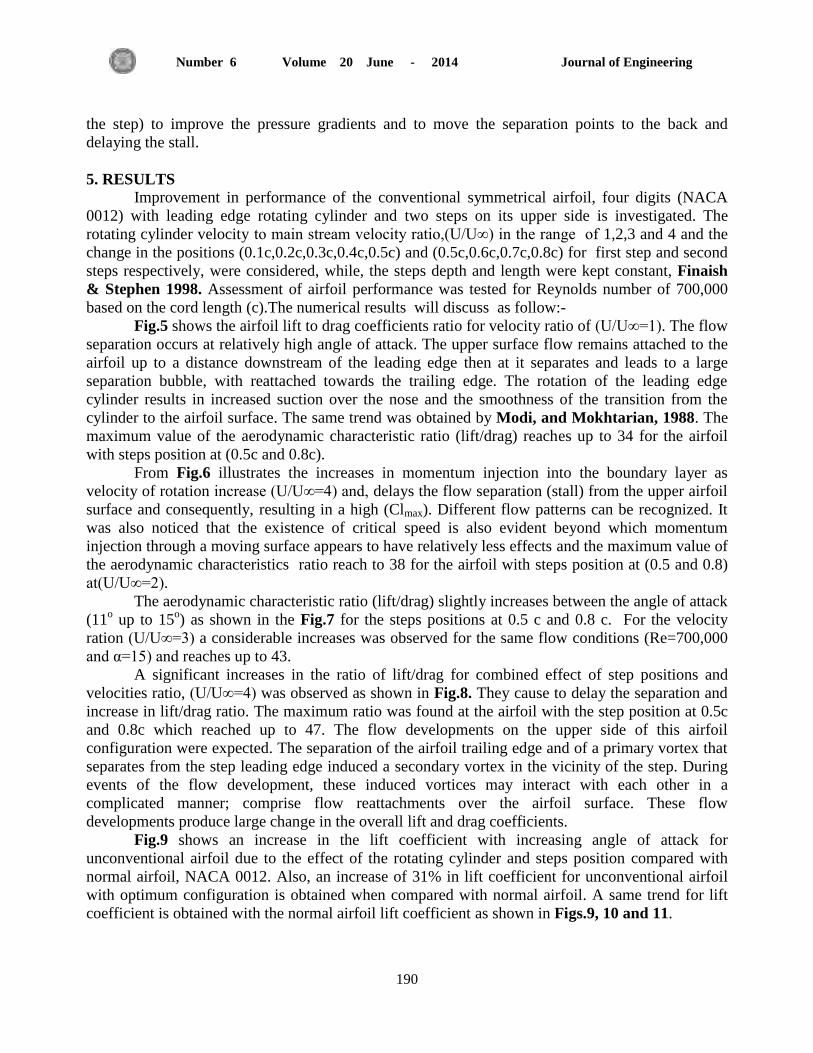
Journal of Engineering Volume 20 June - 2014 Number 6
190
the step) to improve the pressure gradients and to move the separation points to the back and
delaying the stall.
5. RESULTS
Improvement in performance of the conventional symmetrical airfoil, four digits (NACA
0012) with leading edge rotating cylinder and two steps on its upper side is investigated. The
rotating cylinder velocity to main stream velocity ratio,(U/U∞) in the range of 1,2,3 and 4 and the
change in the positions (0.1c,0.2c,0.3c,0.4c,0.5c) and (0.5c,0.6c,0.7c,0.8c) for first step and second
steps respectively, were considered, while, the steps depth and length were kept constant, Finaish
& Stephen 1998. Assessment of airfoil performance was tested for Reynolds number of 700,000
based on the cord length (c).The numerical results will discuss as follow:-
Fig.5 shows the airfoil lift to drag coefficients ratio for velocity ratio of (U/U∞=1). The flow
separation occurs at relatively high angle of attack. The upper surface flow remains attached to the
airfoil up to a distance downstream of the leading edge then at it separates and leads to a large
separation bubble, with reattached towards the trailing edge. The rotation of the leading edge
cylinder results in increased suction over the nose and the smoothness of the transition from the
cylinder to the airfoil surface. The same trend was obtained by Modi, and Mokhtarian, 1988. The
maximum value of the aerodynamic characteristic ratio (lift/drag) reaches up to 34 for the airfoil
with steps position at (0.5c and 0.8c).
From Fig.6 illustrates the increases in momentum injection into the boundary layer as
velocity of rotation increase (U/U∞=4) and, delays the flow separation (stall) from the upper airfoil
surface and consequently, resulting in a high (Clmax). Different flow patterns can be recognized. It
was also noticed that the existence of critical speed is also evident beyond which momentum
injection through a moving surface appears to have relatively less effects and the maximum value of
the aerodynamic characteristics ratio reach to 38 for the airfoil with steps position at (0.5 and 0.8)
at(U/U∞=2).
The aerodynamic characteristic ratio (lift/drag) slightly increases between the angle of attack
(11o up to 15
o) as shown in the Fig.7 for the steps positions at 0.5 c and 0.8 c. For the velocity
ration (U/U∞=3) a considerable increases was observed for the same flow conditions (Re=700,000
and α=15) and reaches up to 43.
A significant increases in the ratio of lift/drag for combined effect of step positions and
velocities ratio, (U/U∞=4) was observed as shown in Fig.8. They cause to delay the separation and
increase in lift/drag ratio. The maximum ratio was found at the airfoil with the step position at 0.5c
and 0.8c which reached up to 47. The flow developments on the upper side of this airfoil
configuration were expected. The separation of the airfoil trailing edge and of a primary vortex that
separates from the step leading edge induced a secondary vortex in the vicinity of the step. During
events of the flow development, these induced vortices may interact with each other in a
complicated manner; comprise flow reattachments over the airfoil surface. These flow
developments produce large change in the overall lift and drag coefficients.
Fig.9 shows an increase in the lift coefficient with increasing angle of attack for
unconventional airfoil due to the effect of the rotating cylinder and steps position compared with
normal airfoil, NACA 0012. Also, an increase of 31% in lift coefficient for unconventional airfoil
with optimum configuration is obtained when compared with normal airfoil. A same trend for lift
coefficient is obtained with the normal airfoil lift coefficient as shown in Figs.9, 10 and 11.

Journal of Engineering Volume 20 June - 2014 Number 6
191
A decrease in drag coefficient is noticed for all values of the velocities ratios as the angle of
attack are increasing. A reduction of 26% in drag coefficient for unconventional airfoil with
optimum configuration is obtained when compared with normal airfoil at the same angle of
attack.as shown in Fig.10. The trend of drag coefficient for unconventional airfoil is similar to drag
coefficient.
The optimum configuration for the unconventional airfoil is found to be at velocities ratio
(U/U∞=4) with the steps position at 0.5c and 0.8c as shown in Fig.11. A high ratio of lift to drag
was observed compared with the same airfoil without leading edge rotating cylinder and steps on
the its upper side.
6. CONCLUSIONS
- The rotating cylinder considered to be the best and effective flow control device which was
controlling the stall of airfoil flow. The large separation region on stalled airfoil can be
reduced significantly by using the rotating cylinder and two upper steps.
- The stalled airfoil flow is sensitive to rotating cylinder speed ratio (U/U∞).
- The lift coefficient of the airfoil is also increased with increase of angle of the attack.
- The rotating cylinder and upper steps causes a decrease in drag and more increase in lift.
- Lift to drag coefficient values of 34,38,43 and 47 are obtained for velocity ratios (U/U∞)
1,2,3 and 4 respectively
- The optimum configuration for the unconventional airfoil is found to be at velocities ratio
(U/U∞=4) with the steps positions at 0.5c and 0.8c for best airfoil performance.
- Normal airfoil separates at angle of attack 12o, while unconventional airfoil with optimum
configuration separates at angle of attack 15o.
- An increase of 31% in lift coefficient for unconventional airfoil with optimum configuration
is obtained compared with normal airfoil.
- A reduction of 26% in drag coefficient for unconventional airfoil with optimum
configuration is obtained compared with normal airfoil at the same angle of attack.
NOMENCLATURE:
C : cord (m)
CL: lift coefficient
DL: drag coefficient
: pressure (N/m2)
Re: Reynolds number
U∞: uniform flow velocity (m/s)
Uc: velocity of the rotational cylinder (m/s)
α: angle of attack (Degree)
: viscosity (kg/m.s)
: velocity in tenser notation (m/s)
: position vector in tensor notation (m)
: Kronecker delta
ρ: density (kg/m3)

Journal of Engineering Volume 20 June - 2014 Number 6
192
: shear stress (N/m2)
REFERENCES
- Al- Tornachi, S.J. and Abu- Tabikh, M.I., 1998, Computation of the Flow Around Airfoils
and Wings under High Lift Separated Flow Condition, Dept. of Mechanical Engineer,
University of Technology, Iraq, Journal Eng & technology Vol. 17, No.9.
- Al-Garni, A. Z.,Al-Garni,AM; Ahmed, SA; Sahin, AZ. 2000, Flow Control for an Airfoil
with Leading-Edge Rotation: an Experimental Study, AMER INST AERONAUT
ASTRONAUT, JORNAL OF AIRCRAFT; pp: 617-622; Vol: 37.
- Buckholtz, R.H.,1986, The Functional Role of Wing Corrugations in Living System,
Department of Mechanical Engineering, Columbia University, New Yourk, NY 10027.
- Cichy, D. R., Harris, J. W., and MacKay, J. K., 1972, Flight Tests of a Rotating Cylinder
Flap on a North American Rockwell Yov-10A Aircraft, NASA CR-2135.
- Davidson, L., 2009, An Introduction To Turbulence Models, http://www.tfd.chalmers.se,
16.
- Fathi Finaish and Stephen Witherspoon., 1998, Aerodynamic Performance of an Airfoil with
Step-induced Vortex for Lift Augmentation. Dept. of Mechanical and Aerospace, University
of Missouri, Rolla, MO 65401.
- Favre, A., 1938, Contribution of an Experimental Studies of Three-dimensional
Hydrodynamic, Ph.D Thesis presented to the University of Paris.
- Ferziger, J. H. and Peric, M., 1999, Computational Methods for Fluid Dynamics, 2nd
Edition Springer, Berlin.
- Freymuth, P., Jackson, S., and Bank, W., 1989, Toward Dynamic Separation without
Dynamic Stall. Dept. of Aerospace Engineering Sciences, University of Colorado, Boulder,
CO 80309, USA. Experiments in Fluids. Springer-Verlag,
- Hanaa, A. H., 2006, Numerical and Experimental Investigation on the Effect of Restriction
Shape on Characteristics of Airflow in a Square Duct, Ph.D. thesis, Mech. Eng. Dept., Univ.
of Technology.
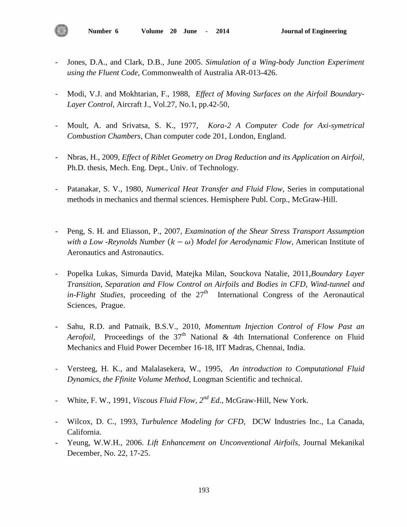
Journal of Engineering Volume 20 June - 2014 Number 6
193
- Jones, D.A., and Clark, D.B., June 2005. Simulation of a Wing-body Junction Experiment
using the Fluent Code, Commonwealth of Australia AR-013-426.
- Modi, V.J. and Mokhtarian, F., 1988, Effect of Moving Surfaces on the Airfoil Boundary-
Layer Control, Aircraft J., Vol.27, No.1, pp.42-50,
- Moult, A. and Srivatsa, S. K., 1977, Kora-2 A Computer Code for Axi-symetrical
Combustion Chambers, Chan computer code 201, London, England.
- Nbras, H., 2009, Effect of Riblet Geometry on Drag Reduction and its Application on Airfoil,
Ph.D. thesis, Mech. Eng. Dept., Univ. of Technology.
- Patanakar, S. V., 1980, Numerical Heat Transfer and Fluid Flow, Series in computational
methods in mechanics and thermal sciences. Hemisphere Publ. Corp., McGraw-Hill.
- Peng, S. H. and Eliasson, P., 2007, Examination of the Shear Stress Transport Assumption
with a Low -Reynolds Number Model for Aerodynamic Flow, American Institute of
Aeronautics and Astronautics.
- Popelka Lukas, Simurda David, Matejka Milan, Souckova Natalie, 2011,Boundary Layer
Transition, Separation and Flow Control on Airfoils and Bodies in CFD, Wind-tunnel and
in-Flight Studies, proceeding of the 27th
International Congress of the Aeronautical
Sciences, Prague.
- Sahu, R.D. and Patnaik, B.S.V., 2010, Momentum Injection Control of Flow Past an
Aerofoil, Proceedings of the 37th
National & 4th International Conference on Fluid
Mechanics and Fluid Power December 16-18, IIT Madras, Chennai, India.
- Versteeg, H. K., and Malalasekera, W., 1995, An introduction to Computational Fluid
Dynamics, the Ffinite Volume Method, Longman Scientific and technical.
- White, F. W., 1991, Viscous Fluid Flow, 2nd
Ed., McGraw-Hill, New York.
- Wilcox, D. C., 1993, Turbulence Modeling for CFD, DCW Industries Inc., La Canada,
California.
- Yeung, W.W.H., 2006. Lift Enhancement on Unconventional Airfoils, Journal Mekanikal
December, No. 22, 17-25.
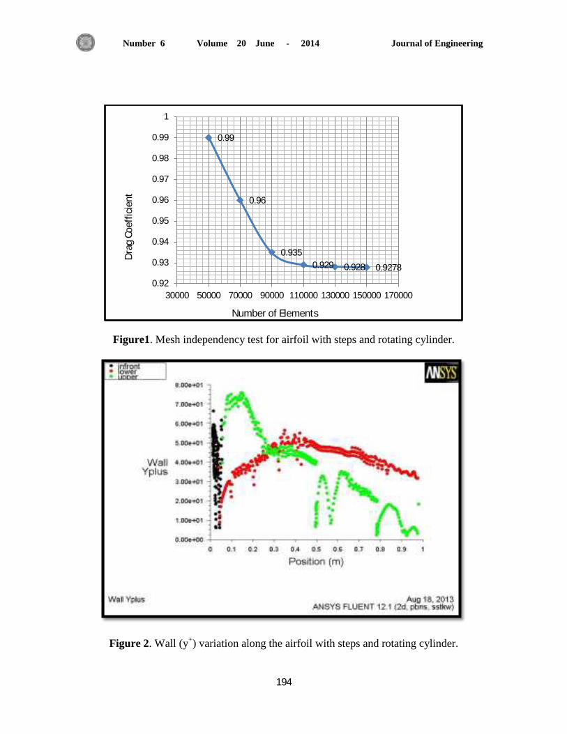
Journal of Engineering Volume 20 June - 2014 Number 6
194
Figure1. Mesh independency test for airfoil with steps and rotating cylinder.
Figure 2. Wall (y+) variation along the airfoil with steps and rotating cylinder.
0.99
0.96
0.935
0.929 0.928 0.9278
0.92
0.93
0.94
0.95
0.96
0.97
0.98
0.99
1
30000 50000 70000 90000 110000 130000 150000 170000
Dra
g C
oef
fici
ent
Number of Elements

Journal of Engineering Volume 20 June - 2014 Number 6
195
Figure3. Mesh on the airfoil surfaces.
Figure4. Geometry and coordinates of the unconventional airfoil consists of front rotating cylinder
and double steps on its upper surface.

Journal of Engineering Volume 20 June - 2014 Number 6
196
Figure 5. Lift to drag coefficient ratio with various angles of attack (α) at velocity ratio (U/U∞=1).
Figure 6. Lift to drag coefficient ratio with various angles of attack (α) at velocity ratio (U/U∞=2).
-5
0
5
10
15
20
25
30
35
40
0 5 10 15 20
Step position(0.3 0.5)
Step position(0.3 0.6)
Step position(0.3 0.7)
Step position(0.3 0.8)
Step position(0.4 0.6)
Step position(0.4 0.7)
Step position(0.4 0.8)
Step position(0.5 0.7)
Step position(0.5 0.8)Lift
Co
effi
cien
t/D
rag
Co
effi
cien
t
Angle of attack (α)
-5
0
5
10
15
20
25
30
35
40
45
0 5 10 15 20
Step position(0.3 0.5)
Step position(0.3 0.6)
Step position(0.3 0.7)
Step position(0.3 0.8)
Step position(0.4 0.6)
Step position(0.4 0.7)
Step position(0.4 0.8)
Step position(0.5 0.7)
Step position(0.5 0.8)Lift
Co
effi
cien
t/D
rag
Co
effi
cien
t
Angle of attack (α)

Journal of Engineering Volume 20 June - 2014 Number 6
197
Figure 7. Lift to drag coefficient ratio with various angles of attack (α) at velocity ratio (U/U∞=3).
Figure 8. Lift to drag coefficient ratio with various angles of attack (α) at velocity ratio (U/U∞=4).
-10
0
10
20
30
40
50
0 5 10 15 20
Step position(0.3 0.5)
Step position(0.3 0.6)
Step position(0.3 0.7)
Step position(0.3 0.8)
Step position(0.4 0.6)
Step position(0.4 0.7)
Step position(0.4 0.8)
Step position(0.5 0.7)
Step position(0.5 0.8)Lift
Co
effi
cien
t/D
rag
Co
effi
cien
t
Angle of attack (α)

Journal of Engineering Volume 20 June - 2014 Number 6
198
Figure 9. Lift coefficient with various angles of attack at steps positions 0.5c and 0.8c.
Figure 10. Drag coefficient with various angles of attack at steps positions 0.5c and 0.8c.
-0.2
0
0.2
0.4
0.6
0.8
1
1.2
1.4
1.6
0 2 4 6 8 10 12 14 16
U/U∞=1
U/U∞=1
U/U∞=3
U/U∞=4
Normal
Lift
co
effi
cien
t (C
l)
Angle of attack (α)
0
0.02
0.04
0.06
0.08
0.1
0.12
0.14
0 5 10 15 20
U/U∞=1
U/U∞=1
U/U∞=3
U/U∞=4
Normal
Angle of attack (α)
Dra
g co
effi
cien
t (C
d)

Journal of Engineering Volume 20 June - 2014 Number 6
199
Figure 11. Lift to drag coefficient ratio with various angles of attack for steps positions at 0.5c and
0.8c.
-10
0
10
20
30
40
50
0 5 10 15 20
U/U∞=1
U/U∞=1
U/U∞=3
U/U∞=4
Normal
Angle of attack (α)
Lift
co
effi
cien
t/D
rag
coef
fici
ent