A New Shift-Share Method∗

Lionel Artige†‡

HEC - University of Liege

Leif van Neuss

HEC - University of Liege

April 11, 2013

Abstract

Shift-share analysis is a decomposition technique widely used in regional studies

to quantify an industry-mix effect and a competitive effect on the growth of regional

employment (or any other relevant variable) relative to the national average. This

technique has always been subject to criticism for its lack of theoretical basis. This

paper presents a critical assessment of the methods suggested by Dunn (1960) and by

Esteban-Marquillas (1972) and proposes a new shift-share method, which separates

out the two effects unambiguously. By way of illustration, we provide an applica-

tion to manufacturing employment in the Belgian provinces between 1995 and 2007.

Keywords: economic structure; regional economics; shift-share; Belgian manu-

facturing employment

JEL Classification: R10, R11, R12, R58

∗We wish to thank Bernard Lejeune for his valuable comments. Responsibility for all errors is ourown.

†L. Artige acknowledges the financial support of the Banque Nationale de Belgique.‡Corresponding author: HEC - University of Liege, Economics Department, Boulevard du Rectorat

7, B31, 4000 Liege, Belgium. E-mail: lionel.artige@ulg.ac.be

1 Introduction

Shift-share analysis is a decomposition technique widely used in regional studies to identify

sectoral effects - the one resulting from the sector’s weights in the economy and the other

from the sectors’ growth rates - leading to inequality in employment growth across regions

(Murray 2010).1 Although the method was developed in the early 1940s, it is generally

attributed to Dunn (1960) in the literature.2 The objective of shift-share analysis is to

compare the sectoral distributions of employment growth between two geographical areas

(usually a region versus the nation as a whole) in order to answer three questions: i)

Does the regional economic structure yield more growth than the national one? ii) Is the

regional sectoral growth higher on average than the national one? iii) From the results to

i) and ii), which one from the structure or the sectoral efficiency contributes more to the

observed differential in aggregate employment growth between the region and the nation?

What shift-share analysis can offer is to propose ordinal variables to answer i) and ii)

and a decomposition technique to answer iii). As the shift-share technique is an account-

ing identity, any formula satisfying this identity is mathematically correct. Therefore,

whereas many decompositions are mathematically possible, only one should answer ques-

tions i), ii) and iii) unambiguously. While various shift-share decompositions have been

proposed in the literature, none is fully convincing yet. The first important decomposition

method was proposed by Dunn (1960), who defines a growth effect from the economic

structure of regional employment - which the literature calls an ”industry-mix effect”

after Esteban-Marquillas (1972) - and finds a residual, which is meant to measure what

Esteban-Marquillas (1972) calls a ”competitive effect” or, for others in the literature, a

1The method has been applied to many other indicators such as income, population and productivity.This paper, like many previous studies using this technique, focuses on employment as this data is easilyavailable at regional level.

2The origins of shift-share decomposition are not too clear as the literature variously attributes itsauthorship. Ray (1990) cites Jones (1940) as the first publication using shift-share analysis.

1

”regional effect”.3 Rosenfeld (1959) soon criticized this residual arguing that the com-

petitive effect in Dunn’s method was not properly defined, as it included some of the

industry-mix effect.4 As a response to this criticism, Esteban-Marquillas (1972) modified

the shift-share technique by adding a third component to construct another competitive

effect. This third component, called the ”allocation effect”, is the residual required by

the accounting identity.

Both methods raised a lot of criticism (Houston (1967); Richardson (1978)). Within this,

we can single out the lack of theoretical foundations (see e.g. Bartels et al. (1982)) and

Cunningham (1969)’s observation that both Dunn and Esteban-Marquillas’ decomposi-

tions yielded two solutions with different values for the industry-mix and competitive

effects. These deficiencies sparked off many shift-share reformulations so as to deepen the

analysis of regional effects of growth (Arcelus 1984); to include interregional and interna-

tional trade flows in the analysis (Sihag & McDonough (1989); Markusen et al. (1991);

Dinc & Haynes (2005)); and to take short-term fluctuations into account within the study

periods (Barff & Knight III 1988). None of these corrections, however, fundamentally de-

parts from the methods of Dunn (1960) and Esteban-Marquillas (1972) as all of these

extensions, in fact, remained based on either.

In the present paper, we argue that the decomposition methods proposed by the shift-

share literature do not solve the methodological problems identified by Rosenfeld (1959)

and Cunningham (1969). In particular, we consider that the definition of the competitive

effect is not only flawed in Dunn (1960) but also in Esteban-Marquillas (1972). As a

result, both methods fail to separate out a structural effect and a competitive effect

relative to the national average. This may lead to incorrect numerical results in empirical

studies and inaccurate policy advice. The contribution of this paper is to provide: 1) a

3Although we prefer ”sectoral efficiency effect” to designate the effect of the sectors’ growth rates, wewill use, in this paper, the term ”competitive effect” as in the literature.

4Dunn’s shift-share method was first published in French (Dunn 1959) with Rosenfeld’s reply appearingin the same publication.

2

comprehensive study of the methods of Dunn (1960) and of Esteban-Marquillas (1972);

2) a test to assess the validity of any shift-share technique and 3) a new technique, which

solves the definitional and technical shortcomings of the traditional shift-share methods.

The paper is organized as follows. Section 2 discusses the usefulness of shift-share anal-

ysis. The methods of Dunn (1960) and of Esteban-Marquillas (1972) are presented and

examined in Section 3 and Section 4 respectively. Section 5 develops a test for shift-share

methods. Section 6 presents a new shift-share decomposition. Section 7 provides an ap-

plication of this new technique to employment variations in the manufacturing sector of

the Belgian provinces between 1995 and 2007 and compares the results with those of the

other two methods. Finally, section 8 presents our conclusions.

2 On the Merits of Shift-Share Analysis

The growth rate of aggregate employment at the regional (or national) level can be disag-

gregated into a sum of sectoral growth rates weighted by the shares of sectors in regional

(or national) employment. The aggregate employment growth performance thus depends

on the economic structure (the weights) and the growth rate of each sector. If we observe

that the growth rate of regional employment is lower than the national one, it can be

interesting to investigate the extent to which the difference is attributable to the effect of

the weights, on the one hand, and to the effect of the mean of the sectoral growth rates,

on the other. This investigation requires to separate the effect of the economic structure

from that of the average growth performance of all sectors.

If there were observable ordinal variables to measure these two effects, regressing the em-

ployment growth differential observed annually between the region and the nation on the

differentials of these two variables would be good enough to realize this investigation.5

5As an alternative to shift-share accounting, Weeden (1974), Buck & Atkins (1976), Berzeg (1978)

3

Such a variable can easily be created in order to measure the effect of the growth per-

formance of sectors: it suffices to take the sum of the sectoral growth rates weighted by

a uniform distribution of sectors, which eliminates any effect of the economic structure.6

Once this variable is avalaible for the region and the nation, the differential between the

two territories can be put in as an explanatory variable.

Yet, there is no obvious way of constructing an ordinal variable to measure the economic

structure because an economic structure defined as the distribution of sectors is not a

variable with an intrinsic ordering. Therefore, taking the difference between the regional

and national distributions of sectors would not make any sense and taking the difference

between the regional and national shares of sectors weighted by a uniform distribution of

sectoral growth rates would necessarily equal zero. The construction of such a variable

thus requires a non-uniform distribution of sectoral growth rates, which means that the

economic structure cannot be isolated from the sectoral growth rates. The question is

then: what non-uniform distribution? As mathematically there is an infinity of non-

uniform distributions of sectoral growth rates, it is impossible to state whether, in total,

the regional or the national economic structure yields more employment growth.

The contribution of shift-share analysis lies in yielding ordinal variables to measure an

effect of the economic structure and an effect of the sectoral growth rates on the observed

differential in aggregate employment growth between two territories. Separating these

two effects clearly amounts to an accounting exercise and shift-share analysis aims at

providing a technique to do so.

and Patterson (1991) have developed econometric analyses of structural effects on regional growth basedon binary variables.

6Let us emphasize that whenever the distribution of sectors is non-uniform the growth performanceof sectors is not purged of any effect of the economic structure.

4

3 Dunn (1960)’s Shift-Share Method

3.1 The Decomposition Method

Shift-share analysis organizes data along three dimensions: geography, sectors of activity

and time. The shift-share method proposed by Dunn (1960) consists in comparing regional

employment growth observed in the data with a hypothetical employment growth that

the region would have experienced, were its growth rate equal to the national one. The

objective of the method is to decompose the difference between these two employment

variations into two components: a structural effect (industry-mix effect) and a competitive

effect.7 Formerly, for a region j, we have8

I∑i=1

(nji,t+1 − nj

i,t)−I∑

i=1

nji,trt+1 =

I∑i=1

nji,t(ri,t+1 − rt+1) +

I∑i=1

nji,t(g

ji,t+1 − ri,t+1) (1)

where nji,t+1 is employment in sector i = 1, ..., I of region j at time t + 1, gji,t+1 is the

employment growth rate between time t and t+1 in sector i of region j, and ri,t+1 and rt+1

are the national employment growth rates between time t and t+1 in, respectively, sector

i and the total economy. The left-hand side of Equation (1) is the difference in observed

and hypothetical regional employment growth between time t and t + 1. On the right-

hand side, the first component (industry-mix effect),∑I

i=1 nji,t(ri,t+1 − rt+1), quantifies

the effect of the economic structure of region j on the regional employment variation

between time t and t+ 1. If employment in all sectors at the national level were to grow

at the rate of national employment or if the regional and national economic structures

were identical, this component would equal zero and the economic structure of region j

7Dunn (1960) refers to the industry-mix and competitive effects respectively as the differential andproportionality effects.

8The development of this decomposition is given in Appendix A.

5

would not matter for employment growth. The second component (competitive effect),∑Ii=1 n

ji,t(g

ji,t+1 − ri,t+1), quantifies the effect of the relative sectoral growth performance

of region j on regional employment variation between time t and t + 1. In order for this

component to equal zero, the employment growth rates in each sector would need to be

the same at the regional and national levels.

If we want to express the difference between observed and hypothetical regional employ-

ment growth in terms of percentage change, we divide Equation (1) by∑I

i=1 nji,t and

obtain

gjt+1 − rt+1 =

∑Ii=1 n

ji,t(ri,t+1 − rt+1)∑I

i=1 nji,t

+

∑Ii=1 n

ji,t(g

ji,t+1 − ri,t+1)∑I

i=1 nji,t

(2)

where gjt+1 =∑I

i=1(nji,t+1−nj

i,t)∑Ii=1 n

ji,t

is the employment growth rate of region j between time

t and t + 1. The left-hand side of Equation (2) is the difference between the observed

regional and national growth rates, and the two components are now expressed in terms

of percentage change. A better way to understand Dunn (1960)’s decomposition is to

rewrite the industry-mix effect in Equation (2) as:

gjt+1 − rt+1 =

(∑Ii=1 n

ji,tri,t+1∑I

i=1 nji,t

−∑I

i=1 mi,tri,t+1∑Ii=1 mi,t

)+

∑Ii=1 n

ji,t(g

ji,t+1 − ri,t+1)∑I

i=1 nji,t

(3)

where mi,t is the national employment in sector i at time t. To rewrite the industry-mix

effect, we used the fact that∑I

i=1 nji,trt+1∑I

i=1 nji,t

= rt+1 =∑I

i=1 mi,tri,t+1∑Ii=1 mi,t

. Finally, we can rewrite

Equation (3) in terms of shares in total employment in region j and at the national level:

gjt+1 − rt+1 =I∑

i=1

(ωji,t − θi,t)ri,t+1 +

I∑i=1

ωji,t(g

ji,t+1 − ri,t+1) (4)

where ωji,t =

nji,t∑I

i=1 nji,t

is the share of sector i in region j in total employment in region j and

6

θi,t =mi,t∑Ii=1 mi,t

is the share of sector i at the national level in total national employment.

3.2 A Critical Assessment

In Equation (4), the industry-mix effect,∑I

i=1(ωji,t − θi,t)ri,t+1, is obtained by associating

the national sectoral growth rates to the regional and the national economic structures

while the competitive effect,∑I

i=1 ωji,t(g

ji,t+1−ri,t+1), is obtained by associating the regional

economic structure to the regional and national sectoral growth rates. In other words,

this method makes a choice on the territorial basis of the growth rates to compute the

industry-mix effect, and on the basis of the economic structure to compute the competitive

effect. Dunn (1960) chose the national growth rates to calculate the industry-mix effect

and the regional economic structure to calculate the competitive effect. We argue that

this choice is arbitrary. He could equally have chosen the regional growth rates for the

industry-mix effect and the national economic structure for the competitive effect. This

decomposition leads to the same difference between the regional and national employment

growth rate but yields different values for the two effects if the region and the country

have different economic structures and growth rates9:

gjt+1 − rt+1 =I∑

i=1

(ωji,t − θi,t)g

ji,t+1 +

I∑i=1

θi,t(gji,t+1 − ri,t+1) (5)

In the absence of any explicit criterion, there is no a priori reason to prefer one decom-

position to the other.10 Therefore, the shift-share method based on Dunn (1960) cannot

deliver a unique value for each of the two effects.

Moreover, Rosenfeld (1959) emphazised that the competitive effect in Equation (4) was

inconsistent: if two regions have identical sectoral growth rates but different economic

9In Appendix B we show how to move from Equation (4) to Equation (5).10Cunningham (1969) came to the same conclusion.

7

structures they will have different competitive effects, which means that the economic

structure affects the value of the competitive effect. From Equations (4) and (5) it clearly

appears that neither decomposition suppresses all influence of the economic structure on

the competitive effect.

4 Esteban-Marquillas (1972)’s Shift-Share Method11

4.1 The Decomposition Method

When Dunn presented his shift-share method in 1959, Rosenfeld (1959) identified an

inconsistency in his definition of the competitive effect. He showed that if two regions

have identical growth rates by sector but different economic structures, they will have

different competitive effects relative to the national average because the competitive effect

depends on the economic structure. As a result, the competitive effect is not purged of

any industry-mix effect. Esteban-Marquillas (1972) proposed a solution that has since

become the standard shift-share method. His solution computes the competitive effect

as the difference between the sectoral regional and national growth rates weighted by the

national economic structure. This implies the addition of a third component, called the

”allocation” component, to Equation (1). Formerly, we have

I∑i=1

(nji,t+1 − nj

i,t)−I∑

i=1

nji,trt+1 =

I∑i=1

nji,t(ri,t+1 − rt+1) +

I∑i=1

mi,t(gji,t+1 − ri,t+1)

+I∑

i=1

(nji,t −mi,t)(g

ji,t+1 − ri,t+1) (6)

11Although Esteban-Marquillas (1972) gets the credit for the decomposition method into three compo-nents, Cunningham (1969) had actually proposed it three years earlier. For reasons unknown to us, thelatter’s pioneering work is hardly cited.

8

where∑I

i=1 mi,t(gji,t+1 − ri,t+1) is the newly-defined competitive effect and

mi,t =∑I

i=1 nji,t

( ∑Jj=1 n

ji,t∑I

i=1

∑Jj=1 n

ji,t

)is the ”homothetic employment”, i.e., the hypothetical

employment that region j would have, were its economic structure identical to the na-

tional one. The last term in Equation (6) is the allocation effect, i.e., the product of

the difference between the observed and hypothetical economic structure of region j and

the difference between the regional and national employment growth rate in sector i.

In applied papers, the economic interpretation of the allocation effect is evasive and of-

ten omitted. In their original works, both Esteban-Marquillas (1972) and Cunningham

(1969) interpret a positive allocation effect as the contribution of regional specialization in

sectors in which the regional growth rates are relatively the highest, and a negative allo-

cation effect as a lack of regional specialization in the fastest growing sectors. In addition,

Cunningham (1969) hints that the allocation effect can be indicative of a convergence

(negative allocation effect) or a divergence (positive allocation effect) of the regional and

the national economic structures.

In order to better understand the solution proposed by Esteban-Marquillas (1972), let us

divide Equation (6) by∑I

i=1 nji,t in order to rewrite it in terms of percentage change

gjt+1 − rt+1 =

∑Ii=1 n

ji,t(ri,t+1 − rt+1)∑I

i=1 nji,t

+

∑Ii=1 mi,t(g

ji,t+1 − ri,t+1)∑I

i=1 nji,t

+

∑Ii=1(n

ji,t −mi,t)(g

ji,t+1 − ri,t+1)∑I

i=1 nji,t

(7)

and, then, in terms of employment shares:

gjt+1−rt+1 =I∑

i=1

(ωji,t−θi,t)ri,t+1+

I∑i=1

θi,t(gji,t+1−ri,t+1)+

I∑i=1

(ωji,t−θi,t)(g

ji,t+1−ri,t+1) (8)

9

4.2 A Critical Assessment

We argue that Esteban-Marquillas (1972)’s decomposition method brings no improvement

to Dunn (1960)’s for the following three reasons:

1. This method does not solve the main problem posed by the absence of unique values

for the industry-mix and competitive effects in Dunn (1960)’s method. By compar-

ing Equation (4) with Equation (8), we can observe that the solution proposed

by Esteban-Marquillas (1972) uses the same territorial basis to compute the two ef-

fects: the national growth rates to compute the industry-mix effect and the national

economic structure to compute the competitive effect. Not only is this choice arbi-

trary but it also requires a residual term (allocation effect) to satisfy the equality.

It would have been possible to use the regional territorial basis to compute both

effects, which requires the same allocation effect:12

gjt+1−rt+1 =I∑

i=1

(ωji,t−θi,t)g

ji,t+1+

I∑i=1

ωji,t(g

ji,t+1−ri,t+1)−

I∑i=1

(ωji,t−θi,t)(g

ji,t+1−ri,t+1)

(9)

Equation (9) changes the territorial basis of the sectoral growth rates in Equation

(5) to compute an industry-mix effect with the same territorial basis as in the

competitive effect, and adds a residual term to satisfy the equality. The values

of the two effects are different between Equations (8) and (9) while the residual

terms - the allocation effects - are of opposite signs. The allocation effect allows the

modification of the competitive effect in Equation (8) and of the industry-mix effect

in Equation (9). No more than Dunn’s solution can Esteban-Marquillas’ deliver a

12As Esteban-Marquillas (1972) looked for a competitive effect that would not vary for two regionswith the same sectoral growth rates, Equation (8) is the most appropriate one. From a theoretical pointof view, though, it is no longer justified to use Equation (8) rather than Equation (9).

10

unique value for the industry-mix and competitive effects.13

2. This method is unnecessary to solve the inconsistent example identified by Rosenfeld

(1959). In fact, this inconsistency can be solved without adding a third component

by Equation (5). Let us recall that Equation (5) is:

gjt+1 − rt+1 =I∑

i=1

(ωji,t − θi,t)g

ji,t+1 +

I∑i=1

θi,t(gji,t+1 − ri,t+1)

where∑I

i=1 θi,t(gji,t+1−ri,t+1) is the same competitive effect as the one constructed by

Esteban-Marquillas (1972) in Equation (8). To the best of our knowledge, nobody

has yet thought of this solution to Rosenfeld’s inconsistent example. Nevertheless,

contrary to what is commonly believed, the solution proposed by Esteban-Marquillas

(1972) does not solve the inconsistency identified by Rosenfeld as the former does

not succeed in removing any influence of the economic structure on the computation

of the competitive effect.

3. This method adds a problematic residual term (allocation effect). First, it is unnec-

essary (see previous point). Second, when its value is different from zero, the value

of the competitive effect is necessarily different from that of Dunn’s method based

on Equation (4), and the value of the industry-mix effect is different from that of

Dunn’s method based on Equation (5). How to justify this unless one proves that

Dunn’s method is wrong? Third, the economic interpretation of this allocation ef-

fect given by Esteban-Marquillas (1972) and Cunningham (1969) refers to an effect

of the economic structure, which should in fact be captured by the industry-mix

effect in the first place.

13Once again, Cunningham (1969) came to the same conclusion.

11

We can conlude that Esteban-Marquillas (1972)’s method does not bring any improve-

ment to Dunn (1960)’s. In the next two sections, we propose a simple test to identify a

relevant shift-share method and then propose a new technique. We show that whereas

both Esteban-Marquillas (1972)’s and Dunn (1960)’s methods fail this test, our technique

comes out successfully.

5 A Shift-Share Test

Shift-share analysis aims at answering the following question: does a region’s economic

structure impact its growth performance positively or negatively? If it does negatively,

the effect of the structure may be offset by the average growth performance of all sectors.

Therefore, it would be interesting to discover whether the economic structure of a region

is a relative strength (or weakness) in terms of growth and whether this strength (or

weakness) is reinforced or offset by relatively higher (or lower) sectoral efficiency. A

shift-share technique should be able to separate out these two effects unambiguously.

5.1 Two Difficulties

The first difficulty to tackle in shift-share analysis is the absence of order for an economic

structure. What we call an economic structure is a distribution of sectors with no intrinsic

ordering. A region may specialize in some sectors more than others. We will say that a

region or a nation specializes in a given sector if its employment share is larger than the

uniform share. There is no a priori good or bad specialization. The regional specialization

may be different from the national one but, without considering an associated variable,

it is impossible to conclude that the regional specialization is better than the national

one. Moreover, the specialization may vary between the region and the nation while their

distribution of employment across sectors may be identical. For instance, employment

12

shares can be 20% in sector A and 80% in sector B for the region while being the opposite

for the nation. Although the distributions of employment shares are identical, the regional

and national specializations are different.

When the distribution of sectors is associated with their corresponding sectoral growth

rates, it is possible to conclude that a specialization will yield more or less employment

growth. Yet, another difficulty arises if we want to disentangle the effect of specialization

from the effect of growth rates. This is precisely the objective of shift-share analysis.

We will now show that neither of the methods proposed by Dunn (1960) and Esteban-

Marquillas (1972) solves this difficulty.

5.2 A Simple Shift-Share Test

Table 1 presents two numerical examples. In Example 1, the region and the nation are

identical in all respects: the economic structures and the growth rates are the same for

each sector. Obviously, there is no difference between regional and national employment

growth, and any shift-share technique should find zero industry-mix and competitive

effects. Table 2 shows that the shift-share techniques of Dunn (1960) and Esteban-

Marquillas (1972) find the expected results. In Example 2, we keep the same pairs of

data (employment shares and growth rates) as in Example 1 but assign them to different

sectors between the two geographical units. The distribution of shares and growth rates

is exactly the same as previously but the specializations are now different: the region

specializes in Sector B while the nation does in Sector A. The difference between the

regional and national growth rates between t and t + 1 should be zero. Moreover, any

shift-share technique should conclude that the industry-mix and the competitive effects

are null. Each geographical unit specializes in the highest performing sector and none

has a systematic advantage in employment performance in all sectors. We can observe

that the shift-share techniques of both Dunn (1960) and of Esteban-Marquillas (1972)

13

fail this test (Table 2). In fact, by choosing the national growth rates to compute the

industry-mix effect, both techniques implicitly consider that the national specialization

is better than the regional one. In the case, this conclusion turns out to be wrong, as

regional and national employment growth rates are identical.

Table 1: Two numerical examples

Region Nation

Share of total Employment Share of total Employmentemployment growth rate employment growth rate

at t between t and t+ 1 at t between t and t+ 1

Example 1Sector A 80% 5% 80% 5%Sector B 20% 4% 20% 4%Example 2Sector A 20% 4% 80% 5%Sector B 80% 5% 20% 4%

Table 2: Dunn (1960)’s and Esteban-Marquillas (1972)’s shift-share methods under test

Growth rate Industry-mix Competitive Allocationdifferential effect effect effect

(%) (%) (%) (%)

Example 1Dunn’s decomposition 0.0 0.0 0.0 -EM’s decomposition 0.0 0.0 0.0 0.0Example 2Dunn’s decomposition 0.0 -0.6 0.6 -EM’s decomposition 0.0 -0.6 -0.6 1.2

Growth rate differential = difference between the regional and the national aggregate employment growth rates

EM = Esteban-Marquillas’ shift-share method

14

Table 3: Our shift-share method under test

Growth rate Industry-mix Competitivedifferential effect effect

(%) (%) (%)

Example 1Our decomposition 0.0 0.0 0.0Example 2Our decomposition 0.0 0.0 0.0

Growth rate differential = difference between the regional and the national aggregate employment growth rates

6 A New Shift-Share Decomposition

A valid shift-share technique should result in a unique decomposition of the growth dif-

ferential between two geographical units into an industry-mix effect and a competitive

effect. In addition, this technique should solve Rosenfeld’s inconsistency and pass the test

of Example 2. The new technique we now propose provides the solution to separate out

unambiguously an effect of the economic structure and a competitive effect.

Our technique starts with the construction of the competitive effect. Rosenfeld (1959)

rightly pointed out that the competitive effect should not be influenced by the economic

structure if one wanted to separate out an effect from the economic structure and an effect

from the sectoral growth rates. Both Dunn (1960)’s and Esteban-Marquillas (1972)’s

methods fail in building such a competitive effect. As mentioned in Section 2, the only

way to purge the competitive effect from any influence of the economic structure is to

associate a uniform distribution of sectors to the sectoral growth rates. Therefore, we

define the competitive effect as

I∑i=1

1

I

(gji,t+1 − ri,t+1

)(10)

where I is the number of sectors and 1Iis the employment share of each sector. Equation

15

(10) is the difference between the arithmetic means of the regional and national sectoral

growth rates. If Equation (10) is positive, the arithmetic mean of the sectoral growth rates

is higher in the region than in the nation. In that case, the sectors, on average, yield more

growth in the region than in the nation. Then, we calculate the effect of the economic

structure (or the industry-mix effect) as the residual, i.e., as the difference between the

differential in the aggregate employment growth rates (gjt+1− rt+1), on the one hand, and

Equation (10), on the other hand, which yields:

I∑i=1

(ωji,t −

1

I

)gji,t+1 −

I∑i=1

(θi,t −

1

I

)ri,t+1 (11)

where∑I

i=1

(ωji,t − 1

I

)and

∑Ii=1

(θi,t − 1

I

)are the regional and national specialisations

respectively. As mentioned in Section 2, the economic structure is a distribution of sectors

and the difference between these two terms is meaningless. As such, we cannot say

which specialization is better than the other. Yet the specialisations associated with

their corresponding sectoral growth rates, as it comes out in Equation (11), are ordinal

variables measuring employment growth due to specialization. Equation (11) allows us to

determine which of the two specializations yields more employment growth. If Equation

(11) is positive, then the regional economic structure yields more employment growth

than the national one. Our new shift-share decomposition equation thus is the sum of

Equations (10) and (11):

gjt+1 − rt+1 =

[I∑

i=1

(ωji,t −

1

I

)gji,t+1 −

I∑i=1

(θi,t −

1

I

)ri,t+1

]+

I∑i=1

1

I

(gji,t+1 − ri,t+1

)(12)

Equation (12) accounts for the observed difference between the regional and national ag-

gregate employment growth rates and separates out the industry-mix and the competitive

16

effects unambigously. Finally, Table 3 shows that our method passes the shift-share test

as it yields the expected results for the industry-mix and competitive effects in Example

2.

Let us insist that our method is a major departure from the approach commonly used in

the shift-share literature. Dunn (1960) and Esteban-Marquillas (1972) compare an actual

regional growth rate with two hypothetical regional growth rates that would result if the

sectoral growth rates or the economic structure were identical to those of the nation.

Therefore, the actual and hypothetical growth effects of the economic structure and the

sectoral growth rates are mixed up in their decomposition formula. Our method only

uses actual data, computes actual growth effects in both geographical units and compare

them. It enables us to decompose the aggregate growth rate of any geographical unit

into two terms, which capture the two effects we are interested in: the growth effect of

the economic structure and the growth effect of the sectoral growth performances. The

regional and national decompositions are the following:

gjt+1 =I∑

i=1

(ωji,t −

1

I

)gji,t+1 +

I∑i=1

1

Igji,t+1 (13)

rt+1 =I∑

i=1

(θi,t −

1

I

)ri,t+1 +

I∑i=1

1

Iri,t+1 (14)

The growth effect of the economic structure is measured by(∑I

i=1

(ωji,t − 1

I

)gji,t+1

)in

the region and by(∑I

i=1

(θi,t − 1

I

)ri,t+1

)in the nation. It is positive if the territory

specializes, on average, in fast-growing sectors, i.e. in sectors which experience a relative

high growth rate. The growth effect of the sectoral growth performances is measured

by(∑I

i=11Igji,t+1

)in the region and by

(∑Ii=1

1Iri,t+1

)in the nation. Equations (13)

and (14) are independant from each other and can be used to create ordinal variables

17

for the economic structures in the region and in the nation.14 With our new shift-share

decomposition, we can compare the two growth effects of a geographical unit with those

of any other geographical unit without defining a reference territory. For instance, if one

wants to assess whether the specialization of the region is favourable or harmful to its

growth performance, in comparison with the nation, it is enough to compare the growth

effect of the regional economic structure(∑I

i=1

(ωji,t − 1

I

)gji,t+1

)with the growth effect of

the national one(∑I

i=1

(θi,t − 1

I

)ri,t+1

). If one wants to assess the total regional growth

performance in terms of industrial specialization and sectoral efficiency relative to the

nation, one has to take the difference between Equations (13) and (14), which yields

Equation (12).

7 An application to employment in the Belgian man-

ufacturing sector between 1995 and 2007

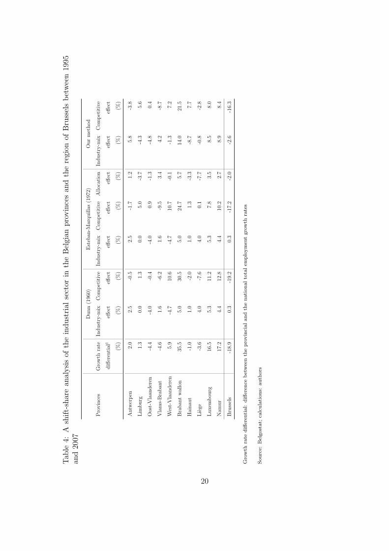
By way of illustration, we propose to carry out a shift-share analysis of employment varia-

tions in the manufacturing sector in the Belgian provinces and the Brussels region between

1995 and 2007, and to compare the results of our technique with those of the traditional

shift-share methods. Data on 14 sub-sectors of the manufacturing sector was retrieved

from the Belgian Central Bank’s database for the 10 Belgian provinces and for Brussels,

as listed in the first column of Table 4. At the national level, data shows that manufac-

turing employment decreased by 13.4% over that period. The second column of the table

displays the employment growth rate differential of each province and Brussels relative

to the national growth rate. We then computed the industry-mix and the competitive

effects using Dunn (1960)’s technique (third and fourth columns), the same two effects

14In growth regressions, it would be possible to use this ordinal variable measuring the growth effectof the economic structure as an explanatory variable.

18

plus the allocation effect using Esteban-Marquillas (1972)’s technique (fifth to seventh

columns) and the industry-mix and the competitive effects using our new technique (last

two columns). This exercise clearly shows that Dunn (1960)’s and Esteban-Marquillas

(1972)’s techniques can lead to very misleading measures of the competitive and the

industry-mix effects. For instance, in the province of Liege, where employment fell 3.6%

under the national average, the industry-mix effect and the competitive effect amount

to respectively 4.0% and -7.6% with Dunn (1960)’s method, as against 4.0% and 0.1%

(while the allocation effect reaches -7.7%) with Esteban-Marquillas (1972)’s method, and

-0.8% and -2.8% with our own method. In terms of policy prescriptions, the conclusions

based on our decomposition technique stood in clear contrast with those of Dunn (1960)

and of Esteban-Marquillas (1972): the economic structure of the Province of Liege does

not provide it with a relative structural advantage in terms of employment growth. In

light of these comparative evidence, we recommend the use of our technique in shift-share

studies.

19

Tab

le4:

Ashift-sharean

alysisof

theindustrial

sector

intheBelgian

provincesan

dtheregion

ofBrusselsbetween1995

and2007

Dunn(1960)

Esteban

-Marquillas(1972)

Ourmethod

Provinces

Growth

rate

Industry-m

ixCom

petitive

Industry-m

ixCom

petitive

Allocation

Industry-m

ixCom

petitive

differential

1eff

ect

effect

effect

effect

effect

effect

effect

(%)

(%)

(%)

(%)

(%)

(%)

(%)

(%)

Antw

erpen

2.0

2.5

-0.5

2.5

-1.7

1.2

5.8

-3.8

Lim

burg

1.3

0.0

1.3

0.0

5.0

-3.7

-4.3

5.6

Oost-Vlaan

deren

-4.4

-4.0

-0.4

-4.0

0.9

-1.3

-4.8

0.4

Vlams-Braban

t-4.6

1.6

-6.2

1.6

-9.5

3.4

4.2

-8.7

West-Vlaan

deren

5.9

-4.7

10.6

-4.7

10.7

-0.1

-1.3

7.2

Braban

twallon

35.5

5.0

30.5

5.0

24.7

5.7

14.0

21.5

Hainau

t-1.0

1.0

-2.0

1.0

1.3

-3.3

-8.7

7.7

Liege

-3.6

4.0

-7.6

4.0

0.1

-7.7

-0.8

-2.8

Luxem

bou

rg16.5

5.3

11.2

5.3

7.8

3.5

8.5

8.0

Nam

ur

17.2

4.4

12.8

4.4

10.2

2.7

8.9

8.4

Brussels

-18.9

0.3

-19.2

0.3

-17.2

-2.0

-2.6

-16.3

Growth

rate

differen

tial:

differen

cebetweenth

eprovincialandth

enationaltotalem

ploymen

tgrowth

rates

Source:

Belgostat;

calculations:

auth

ors

20

8 Conclusion

The shift-share method is an accounting technique which aims at determining whether

the aggregate growth performance of a region relative to the national average is the result

of its economic structure or/and the growth rates of its sectors. Hence, the accounting

formula should be able to separate out the two components unambiguously. This paper

attempts to show that the traditional shift-share methods proposed by Dunn (1960) and

Esteban-Marquillas (1972) fail to do so due to a flawed definition of the competitive effect.

Instead of these, the shift-share decomposition technique we recommend here is based on

a competitive effect defined as the sum of the sectoral growth rates weighted by a uniform

distribution of sectors. This is the only way to eliminate any effect of the second com-

ponent, the economic structure, which is computed as the residual. Thus the separation

between the two components is unambiguous.

Since all accounting shift-share methods are mathematically correct, we designed a simple

test to assess the conceptual accuracy of shift-share methods and rule out inaccurate ones.

The test confirms the flaws that we identified in Dunn (1960)’s and Esteban-Marquillas

(1972)’s methods and validates the relevance of our own.

Finally, our empirical application on employment in the Belgian manufacturing sector

between 1995 and 2007 shows that the three methods can yield very different results for

the industry-mix and competitive effects. Even though shift-share analysis does not shed

light on the causes of regional growth, it is very useful in identifying and quantifying these

possible sources of regional growth performance. Therefore, the conceptual accuracy of

the accounting technique is compelling in order to deliver the right assessment in regional

studies.

21

References

Arcelus, F. J. (1984), ‘An extension of shift-share analysis’, Growth and Change 15(1), 3–

8.

Barff, R. A. & Knight III, P. L. (1988), ‘Dynamic shift-share analysis’, Growth and Change

19(2), 1–10.

Bartels, C. P., Nicol, W. R. & van Duijn, J. J. (1982), ‘Estimating the impact of regional

policy: A review of applied research methods’, Regional Science and Urban Economics

12(1), 3 – 41.

Berzeg, K. (1978), ‘The empirical content of shift-share analysis’, Journal of Regional

Science 18(3), 463–469.

Buck, T. W. & Atkins, M. H. (1976), ‘The impact of british regional policies on employ-

ment growth’, Oxford Economic Papers 28(1), 118–132.

Cunningham, N. J. (1969), ‘A note on the ’proper distribution of industry”, Oxford Eco-

nomic Papers 21(1), 122–127.

Dinc, M. & Haynes, K. (2005), ‘Productivity, international trade and reference area inter-

actions in shift-share analysis: Some operational notes’, Growth and Change 36(3), 374–

394.

Dunn, E. S. (1959), ‘Une technique statistique et analytique d’analyse regionale: descrip-

tion et projection’, Economie appliquee 4, 521–530.

Dunn, E. S. (1960), ‘A statistical and analytical technique for regional analysis’, Papers

and Proceedings of the Regional Science Association 6, 97–112.

Esteban-Marquillas, J. M. (1972), ‘A reinterpretation of shift-share analysis’, Regional

and Urban Economics 2(3), 249–261.

22

Houston, D. B. (1967), ‘The shift and share analysis of regional growth: A critique’,

Southern Economic Journal 33(4), 577–581.

Jones, J. (1940), A memorandum on the location of industry, The Royal Commission on

the Distribution of the Industrial Population. London., His Majesty’s Stationery Office,

Cmnd 6135, London.

Markusen, A. R., Noponen, H. & Driessen, K. (1991), ‘International trade, productivity,

and us regional job growth : a shift-share interpretation’, International Regional Science

Review 14(1), 15–39.

Murray, A. T. (2010), ‘Quantitative geography’, Journal of Regional Science 50(1), 143–

163.

Patterson, M. G. (1991), ‘A note on the formulation of a full-analogue regression model

of the shift-share method’, Journal of Regional Science 31(2), 211–216.

Ray, M. (1990), ‘Standardising employment growth rates of foreign multinationals and

domestic firms in canada: from shift-share to multifactor partitioning’, International

Labour Organization Working Paper N 62 .

Richardson, H. H. (1978), ‘The state of regional economics: A survey article’, Interna-

tional Regional Science Review 3(1), 1–48.

Rosenfeld, F. (1959), ‘Commentaire a l’expose de M. Dunn’, Economie Appliquee 4, 531–

534.

Sihag, B. S. & McDonough, C. C. (1989), ‘Shift-share analysis: The international dimen-

sion’, Growth and Change 20(3), 80–88.

Weeden, R. (1974), Regional rates of growth of employment: an analysis of variance

23

treatment, Regional Paper 3, National Institute of Economic and Social Research, Cam-

bridge, U.K.

24

A The original decomposition of Dunn (1960)

Let us define employment in sector i at time t in region j by nji,t and in the nation by

mi,t. Equation (1) is obtained from the difference between the regional and national

employment variations:

∑Ii=1 n

ji,t+1∑I

i=1 nji,t

−∑I

i=1 mi,t+1∑Ii=1 mi,t

= (1 + gjt+1)− (1 + rt+1)

=

∑Ii=1 n

ji,t(1 + gjt+1)∑Ii=1 n

ji,t

−∑I

i=1 nji,t(1 + rt+1)∑Ii=1 n

ji,t

=

∑Ii=1 n

ji,tg

jt+1∑I

i=1 nji,t

−∑I

i=1 nji,trt+1∑I

i=1 nji,t

=

∑Ii=1 n

ji,tg

ji,t+1∑I

i=1 nji,t

−∑I

i=1 nji,trt+1∑I

i=1 nji,t

+

∑Ii=1 n

ji,tr

ji,t+1∑I

i=1 nji,t

−∑I

i=1 nji,tr

ji,t+1∑I

i=1 nji,t

=

∑Ii=1 n

ji,t(ri,t+1 − rt+1)∑I

i=1 nji,t

+

∑Ii=1 n

ji,t(g

ji,t+1 − ri,t+1)∑I

i=1 nji,t

where we used the fact that∑I

i=1 nji,tg

jt+1 =

∑Ii=1 n

ji,tg

ji,t+1.

Therefore, gjt+1 − rt+1 =∑I

i=1 nji,t(ri,t+1−rt+1)∑I

i=1 nji,t

+∑I

i=1 nji,t(g

ji,t+1−ri,t+1)∑I

i=1 nji,t

. By multiplying both

sides by∑I

i=1 nji,t, and taking the fact that

∑Ii=1 n

ji,tg

jt+1 =

∑Ii=1(n

ji,t+1 − nj

i,t), we obtain

Equation (1).

B Two possible decompositions following Dunn (1960)

Equation (4) is the rewriting of the decomposition proposed by Dunn (1960):

25

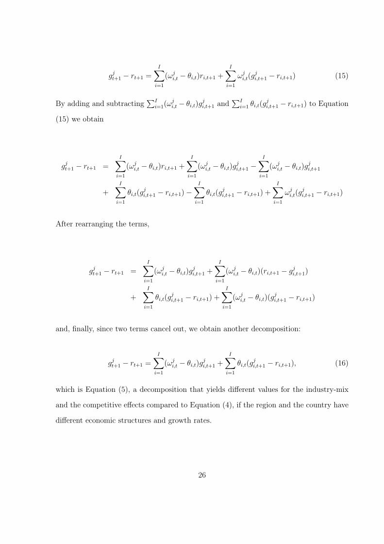
gjt+1 − rt+1 =I∑

i=1

(ωji,t − θi,t)ri,t+1 +

I∑i=1

ωji,t(g

ji,t+1 − ri,t+1) (15)

By adding and subtracting∑I

i=1(ωji,t − θi,t)g

ji,t+1 and

∑Ii=1 θi,t(g

ji,t+1 − ri,t+1) to Equation

(15) we obtain

gjt+1 − rt+1 =I∑

i=1

(ωji,t − θi,t)ri,t+1 +

I∑i=1

(ωji,t − θi,t)g

ji,t+1 −

I∑i=1

(ωji,t − θi,t)g

ji,t+1

+I∑

i=1

θi,t(gji,t+1 − ri,t+1)−

I∑i=1

θi,t(gji,t+1 − ri,t+1) +

I∑i=1

ωji,t(g

ji,t+1 − ri,t+1)

After rearranging the terms,

gjt+1 − rt+1 =I∑

i=1

(ωji,t − θi,t)g

ji,t+1 +

I∑i=1

(ωji,t − θi,t)(ri,t+1 − gji,t+1)

+I∑

i=1

θi,t(gji,t+1 − ri,t+1) +

I∑i=1

(ωji,t − θi,t)(g

ji,t+1 − ri,t+1)

and, finally, since two terms cancel out, we obtain another decomposition:

gjt+1 − rt+1 =I∑

i=1

(ωji,t − θi,t)g

ji,t+1 +

I∑i=1

θi,t(gji,t+1 − ri,t+1), (16)

which is Equation (5), a decomposition that yields different values for the industry-mix

and the competitive effects compared to Equation (4), if the region and the country have

different economic structures and growth rates.

26