LAB MANUAL OF

ALGORITHM ANALYSIS AND DESIGN LAB

ETCS-254

Maharaja Agrasen Institute of Technology, PSP area, Sector – 22, Rohini, New Delhi – 110085

( Affiliated to Guru Gobind Singh Indraprastha University, Kashmere Gate, New Delhi )

INDEX OF THE CONTENTS

1. Introduction to the Algorithm Analysis and Design.

2. Platform used in the Lab.

3. Hardware available in the lab.

4. List of practicals ( as per syllabus prescribed by G.G.S.I.P.U)

(Practicals are divided into seven sections.)

5. Format of the lab record to be prepared by the students.

6. Marking scheme for the practical exam.

7. Steps to be followed (for each practical).

8. Sample programs.

9. List of viva questions.

10. List of advanced practicals.

11. Steps to be followed for advanced practicals.

INTRODUCTION TO ALGORITHM ANALYSIS AND DESIGN LAB

An algorithm, named after the ninth century scholar Abu Jafar Muhammad Ibn Musu Al-Khowarizmi, An algorithm is a set of rules for carrying out calculation either by hand or on a machine.

1. Algorithmic is a branch of computer science that consists of designing and analyzing computer algorithms The “design” pertain to

i. The description of algorithm at an abstract level by means of a pseudo language, and

ii. Proof of correctness that is, the algorithm solves the given problem in all cases.

2. The “analysis” deals with performance evaluation (complexity analysis).

The complexity of an algorithm is a function g(n) that gives the upper bound of the number of operation (or running time) performed by an algorithm when the input size is n.

There are two interpretations of upper bound.

Worst-case ComplexityThe running time for any given size input will be lower than the upper bound except possibly for some values of the input where the maximum is reached.

Average-case Complexity The running time for any given size input will be the average number of operations over all problem instances for a given size.

An algorithm has to solve a problem. An algorithmic problem is specified by describing the set of instances it must work on and what desired properties the output must have.  

We need some way to express the sequence of steps comprising an algorithm. In order of increasing precision, we have English, pseudocode, and real programming languages. Unfortunately, ease of expression moves in the reverse order. In the manual to describe the ideas of an algorithm pseudocodes, algorithms and functios are used.  

In the algorithm analysis and design lab various stratgies such as Divide and conquer techinque , greedy technique and dynamic programming techniques are done. Many sorting algorithms are implemented to analyze the time complexities.String matching algorithms, graphs and spanning tree algorithms are implemented so as to able to understand the applications of various design stratgies.

PLATFORM USED IN THE LAB

Linux (also known as GNU/Linux) is a Unix-like computer operating system. It is one of the most prominent examples of open source development and free software; its underlying source code is available for anyone to use, modify, and redistribute freely.

SIMPLE LINUX COMMANDS

init Allows to change the server boot up on a specific run levelMost common use: init 5This is a useful command, when for instance a servers fails to identify video type, and ends up dropping to the non-graphical boot-up mode (also called runlevel 3).

The server runlevels rely on scripts to basically start up a server with specific processes and tools upon bootup. Runlevel 5 is the default graphical runlevel for Linux servers. But sometimes you get stuck in a different mode and need to force a level. For those rare cases, the init command is a simple way to force the mode without having to edit the inittab file.

cd This command is used to change the directory and using this command will change the location to what ever directory is specified cd hello will change to the directory named hello located inside the current directory cd /home/games will change to the directory called games within the home directory. Any directory can be specified on the Linux system and change to that directory

from any other directory. There are of course a variety of switches associated with the cd command but generally it is used pretty much as it is.

Rm removes /deletes directories and files Most common use: rm -r name (replace name of the file or directory )

The -r option forces the command to also apply to each subdirectory within the directory. For instance to delete the entire contents of the directory x which includes directories y and z this command will do it in one quick process. That is much more useful than trying to use the rmdir command after deleting files! Instead use of rm -r command will save time and effort.

cp The cp command copies files. A file can be copied in the current directory or can be copied to another directory. cp myfile.html /home/help/mynewname.html This will copy the file called myfile.html in the current directory to the directory /home/help/ and call it mynewname.html. Simply put the cp command has the format of cp file1 file2 With file1 being the name (including the path if needed) of the file being copied and file2 is the name (including the path if needed) of the new file being created. The cp command the original file remains in place.

dir The dir command is similar to the ls command only with less available switches (only about 50 compared to about 80 for ls). By using the dir command a list of the contents in the current directory listed in columns can be seen. Type man dir to see more about the dir command.

find The find command is used to find files and or folders within a Linux system. To find a file using the find command find /usr/bin -name filename can be typed. This will search inside the /usr/bin directory (and any sub directories within the /usr/bin directory) for the file named filename. To search the entire filing system including any mounted drives the command used is

find / -name filename and the find command will search every file system beginning in the root directory. The find command can also be used to find command to find files by date and the find command happily understand wild characters such as * and ?

ls The ls command lists the contents of a directory. In its simple form typing just ls at the command prompt will give a listing for the directory currently in use. The ls command can also give listings of other directories without having to go to those directories for example typing ls /dev/bin will display the listing for the directory /dev/bin . The ls command can also be used to list specific files by typing ls filename this will display the file filename (of course you can use any file name here). The ls command can also handle wild characters such as the * and ? . For example ls a* will list all files starting with lower case a ls [aA]* will list files starting with either lower or upper case a (a or A remember linux is case sensitive) or ls a? will list all two character file names beginning with lower case a . There are many switches (over 70) associated with the ls command that perform specific functions. Some of the more common switches are listed here.

ls -a This will list all file including those beginning with the'.' that would normally be hidden from view.

ls -l This gives a long listing showing file attributes and file permissions. ls -s Will display the listing showing the size of each file rounded up to the

nearest kilobyte. ls -S This will list the files according to file size. ls -C Gives the listing display in columns. ls -F Gives a symbol next to each file in the listing showing the file type.

The / means it is a directory, the * means an executable file, the @ means a symbolic link.

ls -r Gives the listing in reverse order. ls -R This gives a recursive listing of all directories below that where the

command was issued. ls -t Lists the directory according to time stamps.

Switches can be combined to produce any output desired. e.g.

ls -la This will list all the files in long format showing full file details.

mkdir The mkdir command is used to create a new directory. mkdir mydir This will make a directory (actually a sub directory) within the current directory called mydir.

mv The mv command moves files from one location to another. With the mv command the file will be moved and no longer exist in its former location prior to the mv. The mv command can also be used to rename files. The files can be moved within the current directory or another directory. cp myfile.html /home/help/mynewname.html This will move the file called myfile.html in the current directory to the directory /home/help/ and call it mynewname.html. The mv command has the format of mv file1 file2

With file1 being the name (including the path if needed) of the file being moved and file2 is the name (including the path if needed) of the new file being created.

rm The rm command is used to delete files. Some very powerful switches can be used with the rm command.To check the man rm file before placing extra switches on the rm command. rm myfile This will delete the file called mydir. To delete a file in another directory for example rm /home/hello/goodbye.htm will delete the file named goodbye.htm in the directory /home/hello/. Some of the common switches for the rm command are

6. rm -i this operates the rm command in interactive mode meaning it prompts before deleting a file. This gives a second chance to say no do not delete the file or yes delete the file. Linux is merciless and once something is deleted it is gone for good so the -i flag (switch) is a good one to get into the habit of using.

7. rm –f will force bypassing any safeguards that may be in place such as prompting. Again this command is handy to know but care should be taken with its use.

8. rm -r will delete every file and sub directory below that in which the command was given. This command has to be used with care as no prompt will be given in most linux systems and it will mean instant good bye to your files if misused.

rmdir The rmdir command is used to delete a directory. rmdir mydir This will delete the directory (actually a sub directory) called mydir.

How to Write, Compile and Run a Simple C Program On Linux System

1.At the command line, pick a directory to save program and enter:

vi firstprog.cNoteAll C source code files must have a .c file extension.All C++ source code files must have .cpp file extension.

2.Enter the following program:

#include <stdio.h>

int main()

{

int index;

for (index = 0; index < 7; index = index + 1)

printf ("Hello World!\n");

return 0;

}

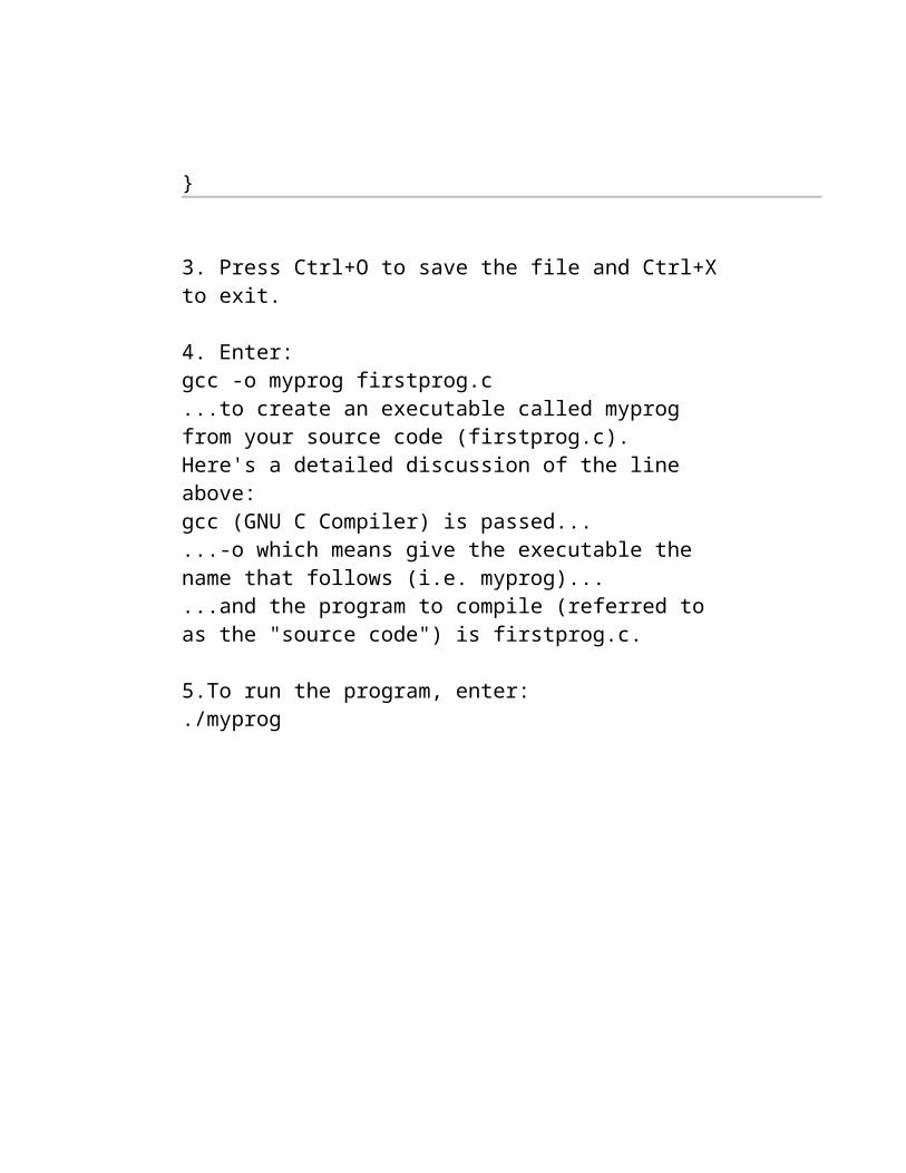
3. Press Ctrl+O to save the file and Ctrl+X to exit.

4. Enter:gcc -o myprog firstprog.c...to create an executable called myprog from your source code

(firstprog.c).Here's a detailed discussion of the line above:gcc (GNU C Compiler) is passed... ...-o which means give the executable the name that follows (i.e. myprog)... ...and the program to compile (referred to as the "source code") is firstprog.c.

5.To run the program, enter:./myprog

HARDWARE AVAILABLE IN THE LAB

CPU HCL {Intel CPU (P-IV 3.0GHz.HT) 512 MB RAM/ 80 GB HDD/ Intel 865 GLC M.B. On Board sound & 3D Graphics Card Lan card key board

MouseCDRW Drive

15’’ Color Monitor UPS

Printer Dot Matrix Printer , 1 LaserJet Printer1160

Software C++ ,Linux

LIST OF PRACTICALS(AS PER GGSIP UNIVERSITY SYLLABUS )

Laboratory Name: Algorithm Analysis And Design Course Code : ETCS 254

SORTING ALGORITHMS:

1. To Analyze time complexity of Insertion sort.2. To Analyze time complexity of Quick sort.3. To Analyze time complexity of Merge sort.

DYNAMIC PROGRAMMING:

4. To Implement Largest Common Subsequence.5. To Implement Optimal Binary Search Tree.6. To Implement Matrix Chain Multiplication.

DIVIDE AND CONQUER TECHNIQUE:

7. To Implement Strassen’s matrix multiplication Algorithm.

GREEDY ALGORITHM’S:

8. To implement Knapsack Problem.9. To implement Activity Selection Problem.

GRAPHS:

10.To implement Dijkstra’s Algorithm.11.To implement Warshall’s Algorithm.12.To implement Bellman Ford’s Algorithm.13.To implement Depth First Search Algorithm.14.To implement Breadth First Search Algorithm.

STRING MATCHING ALGORITHMS:

15.To implement Naïve String Matching Algorithm.16.To implement Rabin Karp String Matching Algorithm

SPANNING TREES:

17.To implement Prim’s Algorithm.18.To implement Kruskal’s Algorithm.

FORMAT OF THE LAB RECORDS TO BE PREPARED BY THE STUDENTS

The students are required to maintain the lab records as per the instructions:

1. All the record files should have a cover page as per the format. 2. All the record files should have an index as per the format.3. All the records should have the following :

I. DateII. Aim

III. Algorithm Or The Procedure to be followed.IV. ProgramV. Output

VI. Viva questions after each section of programs.

MARKING SCHEMEFOR THE

PRACTICAL EXAMINATION

There will be two practical exams in each semester.

Internal Practical Exam External Practical Exam

INTERNAL PRACTICAL EXAMINATION

It is taken by the concerned lecturer of the batch.

MARKING SCHEME FOR INTERNAL EXAM IS:

Total Marks: 40

Division of 40 marks is as follows

1. Regularity: 25

Performing program in each turn of the lab Attendance of the lab File

2. Viva Voice: 10

3. Presentation: 5

NOTE :For the regularity, marks are awarded to the student out of 10 for each experiment performed in the lab and at the end the average marks are given out of 25.

EXTERNAL PRACTICAL EXAMINATION

It is taken by the concerned lecturer of the batch and by an external examiner. In this exam student needs to perform the experiment allotted at the time of the examination, a sheet will be given to the student in which some details asked by the examiner needs to be written and at the last viva will be taken by the external examiner.

MARKING SCHEME FOR THIS EXAM IS:

Total Marks: 60

Division of 60 marks is as follows

1. Sheet filled by the student: 15

2. Viva Voice: 20

3. Experiment performance: 15

4. File submitted: 10

NOTE:

Internal marks + External marks = Total marks given to the students (40 marks) (60 marks) (100 marks)

Experiments given to perform can be from any section of the lab.

STEPS TO BE TAKEN IMPLEMENT PROGRAMMS IN ALGORITHM ANALYSIS AND DESIGN

The programms to be done in the lab are divided in seven sections.

The first section is about complexities of various sorting algorithms. Best, Average and Worst case coplexities of insertion ,quick and merge sort techniques are

compared by plotting graph for varing input sizes and time required by the particular algorithm.

The second section is about dynamic progarmming technique.Dynamic programming solves problems by combining the solution of sub problems. It is only applicable when sub problems are not independent, that is, they share sub sub-Problems. Each time a new sub problem is solved, its solution is stored such that other sub problems sharing the stored sub problem can use the stored value instead of doing a recalculation, thereby saving work compared to applying the divide-and-conquer principle on the same problem which would have recalculated everything. 

The third section is about divide and conquer technique. To use divide and conquer as an algorithm design technique,the problem must be divided into two smaller subproblems, solve each of them recursively, and then meld the two partial solutions into one solution to the full problem. Whenever the merging takes less time than solving the two subproblems, we get an efficient algorithm. Mergesort is the classic example of a divide-and-conquer algorithm. It takes only linear time to merge two sorted lists of n/2 elements each of which was obtained in time. Divide and conquer is a design technique with many important algorithms to its credit, including mergesort, the fast Fourier transform, and Strassen's matrix multiplication algorithm.

The fourth section is about Greedy strategy of designing algorithms. In greedy strategy algorithm always takes the best immediate, or local, solution while finding an answer. Greedy algorithms find the overall, or globally, optimal solution for some optimization problems, but may find less-than-optimal solutions for some instances of other problems.

The fifth section is related to graphs. A graph is a kind of data structure , that consists of a set of nodes and a set of edges that establish relationships (connections) between the nodes.

The sixth section is about string matching algorithms .The problem of string matching is a prevalent and important problem in computer science today. The problem is to search for a pattern string, pat[1..m], in a text string txt[1..n].

Usually n>>m, and txt might be very long indeed, although this is not necessarily so.

The seventh section is about spanning tree. One application of spanning tree could be a cable TV company laying cable to a new neighborhood. If it is constrained to bury the cable only along certain paths, then there would be a graph representing which points are connected by those paths. Some of those paths might be more expensive, because they are longer, or require the cable to be buried deeper; these paths would be represented by edges with larger weights. A spanning tree for that graph would be a subset of those paths that has no cycles but still connects to every house. A minimum spanning tree or minimum weight spanning tree is a spanning tree with weight less than or equal to the weight of every other spanning tree. More generally, any undirected graph has a minimum spanning forest.

SECTION I

ANALSIS OF SORTING TECHNIQUES

ANALYSIS OF SORTING ALGORITHMSBest, Worst, and Average-Case

The worst case complexity of the algorithm is the function defined by the maximum number of steps taken on any instance of size n.  

The best case complexity of the algorithm is the function defined by the minimum number of steps taken on any instance of size n.   The average-case complexity of the algorithm is the function defined by an average number of steps taken on any instance of size n.   Each of these complexities defines a numerical function - time vs. size.

INSERTION SORT

Insertion sort is a simple sorting algorithm that is relatively efficient for small lists and mostly-sorted lists, and often is used as part of more sophisticated algorithms. It works by taking elements from the list one by one and inserting them in their correct position into new sorted list. In arrays, the new list and the remaining elements can share the array's space, but insertion is expensive, requiring shifting

all following elements over by one. The insertion sort works just like its name suggests - it inserts each item into its proper place in the final list. The simplest implementation of this requires two list structures - the source list and the list into which sorted items are inserted. To save memory, most implementations use an in-place sort that works by moving the current item past the already sorted items and repeatedly swapping it with the preceding item until it is in place. Shell sort a variant of insertion sort that is more efficient for larger lists.

Analysis of Insertion Sort

Count the number of times each line of pseudocode will be executed.

Line InsertionSort(A) #Inst. #Exec.

1 for j:=2 to len. of A do c1 n

2 key:=A[j] c2 n-1

3 /* put A[j] into A[1..j-1] */ c3=0 /

4 i:=j-1 c4 n-1

5 while do c5 tj

6 A[i+1]:= A[i] c6

7 i := i-1 c7

8 A[i+1]:=key c8 n-1

The for statement is executed (n-1)+1 times. Within the for statement, "key:=A[j]" is executed n-1 times.

Steps 5, 6, 7 are harder to count. Let the number of elements that have to be slide right to insert the jth item. Step 5 is executed times. Step 6 is . Add up the executed instructions for all pseudocode lines to get the run-time of the algorithm:

What are the ? They depend on the particular input.

Best Case

If it's already sorted, all 's are 1. Hence, the best case time is

where C and D are constants.

Worst CaseIf the input is sorted in descending order, we will have to slide all of the already-sorted elements, so , and step 5 is executed

MERGE SORT

Merge sort takes advantage of the ease of merging already sorted lists into a new sorted list. It starts by comparing every two elements (i.e. 1 with 2, then 3 with 4...) and swapping them if the first should come after the second. It then merges each of the resulting lists of two into lists of four, then merges those lists of four, and so

on; until at last two lists are merged into the final sorted list. Of the algorithms described here, this is the first that scales well to very large lists.

Merge sort works as follows:

1. Divide the unsorted list into two sub lists of about half the size 2. Sort each of the two sub lists 3. Merge the two sorted sub lists back into one sorted list. Pseudocode for mergesort

mergesort(m) var list left, right if length(m) ≤ 1 return m else middle = length(m) / 2 for each x in m up to middle add x to left for each x in m after middle add x to right left = mergesort(left) right = mergesort(right) result = merge(left, right) return result

There are several variants for the merge() function, the simplest variant could look like this:

Pseudocode for merge

merge(left,right) var list result while length(left) > 0 and length(right) > 0 if first(left) ≤ first(right) append first(left) to result left = rest(left) else append first(right) to result right = rest(right) if length(left) > 0 append left to result if length(right) > 0 append right to result return result

ANALYSIS

The straightforward version of function merge requires at most 2n steps (n steps for copying the sequence to the intermediate array b, and at most n steps for copying it back to array a). The time complexity of mergesort is therefore

T(n)   2n + 2 T(n/2)   and

T(1)  =  0

The solution of this recursion yields

T(n)   2n log(n)     O(n log(n))

Thus, the Mergesort algorithm is optimal, since the lower bound for the sorting problem of Ω(n log(n)) is attained.

In the more efficient variant, function merge requires at most 1.5n steps (n/2 steps for copying the first half of the sequence to the intermediate array b, n/2 steps for copying it back to array a, and at most n/2 steps for processing the second half).

This yields a running time of mergesort of at most 1.5n log(n) steps. Algorithm Mergesort has a time complexity of Θ(n log(n)) which is optimal.

A drawback of Mergesort is that it needs an additional space of Θ(n) for the temporary array b.

 

MERGE SORT TREE

QUICK SORT

Quicksort is a divide and conquer algorithm which relies on a partition operation: to partition an array,an element, called a pivot is choosen,all smaller elements are moved before the pivot, and all greater elements are moved after it. This can be done efficiently in linear time and in-place. Then recursively sorting can be done for the lesser and greater sublists. Efficient implementations of quicksort (with in-place partitioning) are typically unstable sorts and somewhat complex, but are among the fastest sorting algorithms in practice. Together with its modest O(log n) space usage, this makes quicksort one of the most popular sorting algorithms, available in many standard libraries. The most complex issue in quicksort is choosing a good pivot element; consistently poor choices of pivots can result in drastically slower (O(n2)) performance, but if at each step we choose the median as the pivot then it works in O(n log n).Quicksort sorts by employing a divide and conquer strategy to divide a list into two sub-lists.

Pick an element, called a pivot, from the list. Reorder the list so that all elements which are less than pivot come before the pivot and so that all elements greater than the pivot come after it (equal values can go either way). After this partitioning, the pivot is in its final position. This is called the partition operation.

Recursively sort the sub-list of lesser elements and the sub-list of greater elements.

Pseudocode For partition(a, left, right, pivotIndex)

pivotValue := a[pivotIndex] swap(a[pivotIndex], a[right]) // Move pivot to end storeIndex := left for i from left to right-1 if a[i] ≤ pivotValue swap(a[storeIndex], a[i]) storeIndex := storeIndex + 1 swap(a[right], a[storeIndex]) // Move pivot to its final place return storeIndex

Pseudocode For quicksort(a, left, right)

if right > left select a pivot value a[pivotIndex] pivotNewIndex := partition(a, left, right, pivotIndex) quicksort(a, left, pivotNewIndex-1) quicksort(a, pivotNewIndex+1, right)

ANALYSISThe partition routine examines every item in the array at most once, so complexity is clearly O(n). Usually, the partition routine will divide the problem into two roughly equal sized partitions. We know that we can divide n items in half log2n times.

This makes quicksort a O(nlogn) algorithm - equivalent to heapsort.

SECTION II

DYNAMIC PROGRAMING TECHNIQUE

DYNAMIC PROGRAMMING

Dynamic Programming is a technique for computing recurrence relations efficiently by sorting partial results. Dynamic programming is a technique for efficiently computing recurrences by storing partial results.

Once dynamic programming is understood, it is usually easier to reinvent certain algorithms . A dynamic programming solution has three components: 

1. Formulate the answer as a recurrence relation or recursive algorithm. 2. Show that the number of different instances of your recurrence is bounded

by a polynomial. 3. Specify an order of evaluation for the recurrence so you always have what

you need.

LONGEST COMMON SUBSEQUENCE PROBLEM

The longest common subsequence problem (LCS) is finding a longest sequence which is a subsequence of all sequences in a set of sequences (often just two). The problem is sometimes defined to be finding all longest common subsequences.It should not be confused with the longest common substring problem (a substring is necessarily a contiguous part).

Solution for two sequences

Given the sequences and

Here + denotes concatenation, and max' gives the longest sequence.Since this problem has an optimal substructure property, it can be solved by dynamic programming.The rationale for this recurrence is that, if the last character of two sequences are equal, they must be part of the LCS. A larger LCS can never be obtained by matching xm to yj where j < n, and vice versa. To find all the longest common subsequences, the LCS should be denoted as a set of sequences, and 'max should return both solutions if they are equally long.

COMPUTING THE LENGTH OF THE LCSThe below function takes as input sequences X[1..m] and Y[1..n] computes the LCS between X[1..i] and Y[1..j] for all 1 ≤ i ≤ m and 1 ≤ j ≤ n, and stores it in C[i,j]. C[m,n] will contain the length of the LCS of X and Y.

function LCS(X[1..m], Y[1..n]) C = array(0..m, 0..n) for i := 1..m for j := 1..n if X[i] = Y[j] C[i,j] := C[i-1,j-1] + 1 else: C[i,j] := max(C[i,j-1], C[i-1,j]) return C

The following function backtracks the choices taken when computing the C table. If the last characters in the prefixes are equal, they must be in an LCS. If not, check what gave the largest LCS of keeping xi and yj, and make the same choice. Just choose one if they were equally long. Call the function with i=m and j=n.function backTrack(C[0..m,0..n], X[1..m], Y[1..n], i, j) if i = 0 or j = 0 return "" else if X[i] = Y[j] return backTrack(C, X, Y, i-1, j-1) + X[i] else if C[i,j-1] > C[i-1,j] return backTrack(C, X, Y, i, j-1) else return backTrack(C, X, Y, i-1, j)

If choosing xi and yj would give an equally long result, both resulting subsequences should be shown. This is returned as a set by this function. Notice that this function is not polynominal, as it might branch in almost every step if the strings are similar.

function backTrackAll(C[0..m,0..n], X[1..m], Y[1..n], i, j) if i = 0 or j = 0 return {} else if X[i] = Y[j]: return {Z + X[i-1] for all Z in backTrackAll(C, X, Y, i-1, j-1)} else: R := {} if C[i,j-1] ≥ C[i-1,j]: R := R backTrackAll(C, X, Y, i, j-1)∪ if C[i-1,j] ≥ C[i,j-1]: R := R backTrackAll(C, X, Y, i-1, j)∪ return R

OPTIMAL BINARY SEARCH TREESA binary search tree is a tree where the key values are stored in the internal nodes, the external nodes (leaves) are null nodes, and the keys are ordered lexicographically.i.e. for each internal node all the keys in the left subtree are less than the keys in the node, and all the keys in the right subtree are greater. When we know the probabilities of searching each one of the keys, it is quite easy to compute the expected cost of accessing the tree. An OBST is a BST which has minimal expected cost.

Example: Key -5 1 8 7 13 21

Probabilities 1/8 1/32 1/16 1/32 1/4 1/2

The expectation-value of a search is:

It's clear that this tree is not optimal. - It is easy to see that if the 21 is closer to the root, given its high probability, the tree will have a lower expected cost.

CRITERION FOR AN OPTIMAL TREE Each optimal binary search tree is composed of a root and (at most) two optimal sub trees, the left and the right. The criterion for optimality gives a dynamic programming algorithm. For the root (and each node in turn) there are n possibilities to select one value .Once this choice is made, the set of keys which go into the left sub tree and right sub tree is completely defined, because the tree is lexicographically ordered. The left and right sub trees are now constructed recursively (optimally). This gives the recursive definition of the optimum cost: Let denote the probability of accessing key , let denote the sum of the probabilities from to

The explanation of the formula is easy once we see that the first term corresponds to the left sub tree, which is one level lower than the root, the second term corresponds to the root and the 3 to the right sub tree. Every cost is multiplied by its probability. For simplicity we set and so simplifies to

. This procedure is exponential if applied directly. However, the optimal trees are only constructed over contiguous sets of keys, and there are at

most different sets of contiguous keys. In this case the optimal cost of a sub tree in a matrix T .The Matrix-entry will contain the cost of an optimal sub tree constructed with the keys to The matrix is filled diagonal by diagonal. It is customary to fill the matrix with

that a lot of multiplications and divisions can be saved. Let then

An optimal tree with one node is just the node itself (no other choice), so the diagonal of is easy to fill: .

The cost of the is in ( in our example) And you can see, that it is practical, not to work with the probabilities, but with the frequencies (i.e the probabilities times the least common multiple of their denominators) to avoid fractions as matrix-entries.

MATRIX CHAIN MULTIPLICATION

PROBLEM: Multiplying a Sequence of Matrices . Suppose a long sequence of matrices .   has to be multipliedMultiplying an matrix by a matrix (using the common algorithm) takes

multiplications.

In matrix multiplication it is better to avoid big intermediate matrices, and since matrix multiplication is associative, we can parenthesise however we want. Matrix multiplication is not communitive, so the order of the matrices can not be permuted without changing the result.

ExampleConsider , where A is , B is , C is , and D is . There are three possible parenthesizations:

The order makes a big difference in real computation. Let M(i,j) be the minimum

number of multiplications necessary to compute . The key observations are

The outermost parentheses partition the chain of matricies (i,j) at some k. The optimal parenthesization order has optimal ordering on either side of k.  

A recurrence for this is:

If there are n matrices, there are n+1 dimensions.

A direct recursive implementation of this will be exponential, since there is a lot of duplicated work as in the Fibonacci recurrence.

Divide-and-conquer is seems efficient because there is no overlap, but ...

There are only substrings between 1 and n. Thus it requires only space to store the optimal cost for each of them. All the possibilities can be represented in a triangle matrix. We can also store the value of k in another triangle matrix to reconstruct to order of the optimal parenthesisation. The diagonal moves up to the right as the computation progresses. On each element of the kth diagonal |j-i| = k.

Pseudocode MatrixOrder

for i=1 to n do M[i, j]=0

for diagonal=1 to n-1

for i=1 to n-diagonal do

j=i+diagonal

faster(i,j)=k

return [m(1, n)]

Pseudocode ShowOrder(i, j)

if (i=j) write ( )

else

k=factor(i, j)

write ``(''

ShowOrder(i, k)

write ``*''

ShowOrder (k+1, j)

write ``)''

SECTION III

DIVIDE AND CONQUER TECHNIQUE

DIVIDE AND CONQUER TECHNIQUE

Divide and conquer was a successful military strategy long before it became an algorithm design paradigm. Generals observed that it was easier to defeat one army of 50,000 men, followed by another army of 50,000 men than it was to beat a single 100,000 man army. Thus the wise general would attack so as to divide the enemy army into two forces and then mop up one after the other.  

To use divide and conquer as an algorithm design technique, we must divide the problem into two smaller subproblems, solve each of them recursively, and then meld the two partial solutions into one solution to the full problem. Whenever the merging takes less time than solving the two subproblems, we get an efficient algorithm.

Divide and conquer is a design technique with many important algorithms to its credit, including mergesort, the fast Fourier transform, and Strassen's matrix multiplication algorithm.

STRASSEN ALGORITHM

In the mathematical discipline of linear algebra, the Strassen algorithm, named after Volker Strassen, is an algorithm used for matrix multiplication. It is asymptotically faster than the standard matrix multiplication algorithm, but slower than the fastest known algorithm.

AlgorithmLet A, B be two square matrices over a field F. We want to calculate the matrix product C as

If the matrices A, B are not of type 2n x 2n we fill the missing rows and columns with zeros.We partition A, B and C into equally sized block matrices

with

then

With this construction we have not reduced the number of multiplications. We still need 8 multiplications to calculate the Ci,j matrices, the same number of multiplications we need when using standard matrix multiplication.

Now comes the important part. We define new matrices

which are then used to express the Ci,j in terms of Mk. Because of our definition of the Mk we can eliminate one matrix multiplication and reduce the number of multiplications to 7 (one multiplications for each Mk) and express the Ci,j as

We iterate this division process n-times until the submatrices degenerate into numbers.Practical implementations of Strassen's algorithm switch to standard methods of matrix multiplication for small enough submatrices, for which they are more efficient; the overhead of Strassen's algorithm implies that these "small enough" submatrices are actually quite large, well into thousands of elements.

ANALYSIS OF STRASSEN ALGORITHM

The standard matrix multiplications takes

multiplications of the elements in the field F. We ignore the additions needed because, depending on F, they can be much faster than the multiplications in computer implementations, especially if the sizes of the matrix entries exceed the word size of the machine.With the Strassen algorithm we can reduce the number of multiplications to

.

The reduction in the number of multiplications however comes at the price at a somewhat reduced numeric stability.

SECTION IV

GREEDY TECHNIQUE

GREEDY ALGORITHMS

Greedy Algorithm works by making the decision that seems most promising at any moment; it never reconsiders this decision, whatever situation may arise later. They take decisions on the basis of information at hand without worrying about the effect these decisions may have in the future. They are easy to invent, easy to implement and most of the time quite efficient. Many problems cannot be solved correctly by greedy approach. Greedy algorithms are used to solve optimization problems.

Characteristics and Features of Problems solved by Greedy Algorithms

To construct the solution in an optimal way, Algorithm maintains two sets. One contains chosen items and the other contains rejected items.

The greedy algorithm consists of four function.

1. A function that checks whether chosen set of items provide a solution. 2. A function that checks the feasibility of a set. 3. The selection function tells which of the candidates is the most promising. 4. An objective function, which does not appear explicitly, gives the value of a

solution.

 Structure Greedy Algorithm

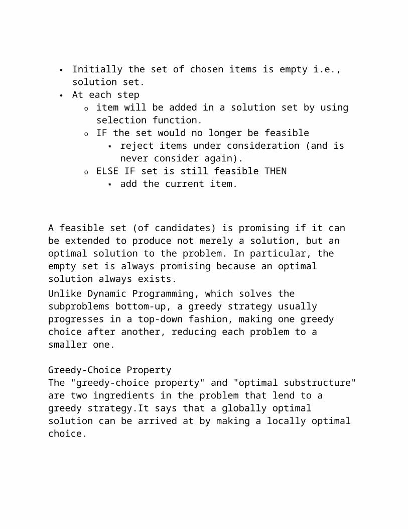
Initially the set of chosen items is empty i.e., solution set. At each step

o item will be added in a solution set by using selection function. o IF the set would no longer be feasible

reject items under consideration (and is never consider again). o ELSE IF set is still feasible THEN

add the current item.

A feasible set (of candidates) is promising if it can be extended to produce not merely a solution, but an optimal solution to the problem. In particular, the empty set is always promising because an optimal solution always exists. Unlike Dynamic Programming, which solves the subproblems bottom-up, a greedy strategy usually progresses in a top-down fashion, making one greedy choice after another, reducing each problem to a smaller one.

Greedy-Choice PropertyThe "greedy-choice property" and "optimal substructure" are two ingredients in the problem that lend to a greedy strategy.It says that a globally optimal solution can be arrived at by making a locally optimal choice.

KNAPSACK PROBLEM

The knapsack problem is a problem in combinatorial optimization. It derives its name from the maximization problem of choosing possible essentials that can fit into one bag (of maximum weight) to be carried on a trip. A similar problem very often appears in business, combinatorics, complexity theory, cryptography and applied mathematics. Given a set of items, each with a cost and a value, then determine the number of each item to include in a collection so that the total cost is less than some given cost and the total value is as large as possible.

Greedy approximation algorithmMartello and Toth (1990) proposed a greedy approximation algorithm to solve the knapsack problem. Their version sorts the essentials in decreasing order and then proceeds to insert them into the sack, starting from the first element (the greatest) until there is no longer space in the sack for more. If k is the maximum possible number of essentials that can fit into the sack, the greedy algorithm is guaranteed to insert at least k/2 of them.

Dynamic Programming for 0-1 Knapsack Problem

For this algorithm let c[i,w] = value of solution for items 1..i and maximum weight w.

c[i,w] = DP-01K(v, w, n, W) 1 for w = 0 to W 2 c[0,w] = 0 3 for i = 1 to n 4 c[i,0] = 0 5 for w = 1 to W

6 if w[i] w 7 then if v[i] + c[i-1,w-w[i]] > c[i-1,w] 8 then c[i,w] = v[i] + c[i-1,w-w[i]] 9 else c[i,w] = c[i-1,w] 10 else c[i,w] = c[i-1,w]

The run time performance of this algorithm is .

AN ACTIVITY SELECTION PROBLEMAn activity-selection is the problem of scheduling a resource among several competing activity. Problem Statement   

Given a set S of n activities with and start time, Si and fi, finish time of an ith activity. Find the maximum size set of mutually compatible activities. Compatible Activities

Activities i and j are compatible if the half-open internal [si, fi) and [sj, fj) do not overlap, that is, i and j are compatible if si ≥ fj  and sj ≥  fi

 

Greedy Algorithm for Selection ProblemI.     Sort the input activities by increasing finishing time.        f1 ≤  f2 ≤  . . . ≤  fn

II.    Call GREEDY-ACTIVITY-SELECTOR (s, f)1. n = length [s] 2. A={i} 3. j = 1 4. for  i = 2  to  n 5.         do if   si ≥ fj 6.              then  A= AU{i} 7.                       j = i 8. return  set A

 

 

Operation of the algorithm

Let 11 activities are given S = {p, q, r, s, t, u, v, w, x, y, z} start and finished times for proposed activities are (1, 4), (3, 5), (0, 6), 5, 7), (3, 8), 5, 9), (6, 10), (8, 11), (8, 12), (2, 13) and (12, 14).

A = {p} Initialization at line 2A = {p, s} line 6 - 1st iteration of FOR - loopA = {p, s, w} line 6 -2nd iteration of FOR - loopA = {p, s, w, z} line 6 - 3rd iteration of FOR-loopOut of the FOR-loop and Return A = {p, s, w, z}

  Analysis

Part I requires O(n lg n) time (use merge of heap sort).Part II requires θ(n) time assuming that activities were already sorted in part I by their finish time.

  CorrectnessNote that Greedy algorithm do not always produce optimal solutions but GREEDY-ACTIVITY-SELECTOR does.

Theorem    Algorithm GREED-ACTIVITY-SELECTOR produces solution of maximum size for the activity-selection problem. Proof

I. Let S = {1, 2, . . . , n} be the set of activities. Since activities are in order by finish time. It implies that activity 1 has the earliest finish time. Suppose, A S is an optimal solution and let activities in A are ordered by finish time. Suppose, the first activity in A is k.If k = 1, then A begins with greedy choice and we are done (or to be very precise, there is nothing to proof here).If k 1, we want to show that there is another solution B that begins with greedy choice, activity 1.Let B =  A - {k} {1}. Because f1   fk, the activities in B are disjoint and since B has same number of activities as A, i.e., |A| = |B|, B is also optimal.

II. Once the greedy choice is made, the problem reduces to finding an optimal solution for the problem. If A is an optimal solution to the original problem S, then A` = A - {1} is an optimal solution to the activity-selection problem S` = {i S: Si   fi}. why? Because if we could find a solution B` to S` with more activities then A`, adding 1 to B` would yield a solution B to S with more activities than A, there by contradicting the optimality. □

   

SECTION V

GRAPHS

GRAPH ALGORITHMS

 Graph Theory is an area of mathematics that deals with following types of problems

Connection problems Scheduling problems Transportation problems Network analysis Games and Puzzles.

The Graph Theory has important applications in Critical path analysis, Social psychology, Matrix theory, Set theory, Topology, Group theory, Molecular chemistry, and Searching.

DIJKSTRA'S ALGORITHMDijkstra's algorithm solves the single-source shortest-path problem when all edges have non-negative weights. It is a greedy algorithm and similar to Prim's algorithm. Algorithm starts at the source vertex, s, it grows a tree, T, that ultimately spans all vertices reachable from S. Vertices are added to T in order of

distance i.e., first S, then the vertex closest to S, then the next closest, and so on. Following implementation assumes that graph G is represented by adjacency lists. 

DIJKSTRA (G, w, s)

1. INITIALIZE SINGLE-SOURCE (G, s) 2. S ← { }     // S will ultimately contains vertices of final shortest-path weights from s 3. Initialize priority queue Q i.e., Q  ←  V[G] 4. while priority queue Q  is not empty do 5.     u  ←  EXTRACT_MIN(Q)    // Pull out new vertex 6.     S  ←  S È {u}     // Perform relaxation for each vertex v

adjacent to u 7.     for each vertex v in Adj[u] do 8.         Relax (u, v, w)

 

ANALYSISLike Prim's algorithm, Dijkstra's algorithm runs in O(|E|lg|V|) time.

 

FLOYD WARSHALL’S ALGORITHM

Floyd warshall algorithm is used to solve the all pairs shortest path problem in a weighted, directed graph by multiplying an adjacency-matrix

representation of the graph multiple times. The edges may have negative weights, but no negative weight cycles.

Steps to implement Floyd Warshall’s algorithm

1. [Initialize matrix m]Repeat through step 2 fir I = 0 ,1 ,2 ,3 ,….., n – 1Repeat through step 2 fir j =0 ,1 ,2 ,3 ,….., n – 1

2. [Test the condition and assign the required value to matrix m]If a [ I ] [j] = 0 M [ I ] [ j ] = infinity ElseM [ I ] [ j ] = a [ I ] [ j ]

3. [ Shortest path evaluation ] Repeat through step 4 for k = 0 , 1 , 2 , 3 , …. , n – 1

Repeat through step 4 for I = 0 , 1 , 2 , 3 , …. , n – 1 Repeat through step 4 for j = 0 , 1 , 2 , 3 , …. , n – 1

4 . If m [ I ] [j] < m [ I ][k] + m[k][j]M[i][ j] = m [ I ] [ j ]

Else M [I ] [ j ] = m [ I ] [ j ] +m [ k] [ j ]

5 . Exit

ANALYSISThe time complexity is Θ (V³).

BELLMAN-FORD ALGORITHM Bellman-Ford algorithm solves the single-source shortest-path problem in the general case in which edges of a given digraph can have negative weight as long as G contains no negative cycles.This algorithm, like Dijkstra's algorithm uses the notion of edge relaxation but does not use with greedy method. Again, it uses d[u] as an upper bound on the distance d[u, v] from u to v.

The algorithm progressively decreases an estimate d[v] on the weight of the shortest path from the source vertex s to each vertex v in V until it achieve the actual shortest-path. The algorithm returns Boolean TRUE if the given digraph contains no negative cycles that are reachable from source vertex s otherwise it returns Boolean FALSE. 

BELLMAN-FORD (G, w, s)

1. INITIALIZE-SINGLE-SOURCE (G, s) 2. for each vertex i = 1 to V[G] - 1 do 3.     for each edge (u, v) in E[G] do 4.         RELAX (u, v, w) 5. For each edge (u, v) in E[G] do 6.     if d[u] + w(u, v) < d[v] then 7.         return FALSE 8. return TRUE

 

ANALYSIS The initialization in line 1 takes (v) time For loop of lines 2-4 takes O(E) time and For-loop of line 5-7 takes O(E)

time.

Thus, the Bellman-Ford algorithm runs in O(E) time. 

TRAVERSAL IN A GRAPH

DEPTH-FIRST SEARCH (DFS) is an algorithm for traversing or searching a graph. Intuitively, one starts at the some node as the root and explores as far as possible along each branch before backtracking.

Formally, DFS is an uninformed search that progresses by expanding the first child node of the graph that appears and thus going deeper and deeper until a goal node is found, or until it hits a node that has no children. Then the search backtracks, returning to the most recent node it hadn't finished exploring. In a non-recursive

implementation, all freshly expanded nodes are added to a LIFO stack for expansion.

Steps for implementing Depth first search

1. Define an array B or Vert that store Boolean values, its size should be greater or equal to the number of vertices in the graph G.

2. Initialize the array B to false 3. For all vertices v in G

if B[v] = falseprocess (v)

4. Exit

DFS algorithm used to solve following problems:

Testing whether graph is connected. Computing a spanning forest of graph.

Computing a path between two vertices of graph or equivalently reporting that no such path exists.

Computing a cycle in graph or equivalently reporting that no such cycle exists.

  ANALYSIS

The running time of DSF is (V + E).    

BREADTH FIRST SEARCH (BFS) is an uninformed search method that aims to expand and examine all nodes of a graph systematically in search of a solution. In other words, it exhaustively searches the entire graph without considering the goal until it finds it.

From the standpoint of the algorithm, all child nodes obtained by expanding a node are added to a FIFO queue. In typical implementations, nodes that have not yet been examined for their neighbors are placed in some container (such as a queue or linked list) called "open" and then once examined are placed in the container "closed".

Steps for implementing Breadth first search

1. Initialize all the vertices by setting Flag = 12. Put the starting vertex A in Q and change its status to the waiting state by

setting Flag = 03. Repeat through step 5 while Q is not NULL4. Remove the front vertex v of Q . process v and set the status of v to the

processed status by setting Flag = -15. Add to the rear of Q all the neighbour of v that are in the ready state by

setting Flag = 1 and change their status to the waiting state by setting flag = 0

6. Exit

Breadth First Search algorithm used in Prim's MST algorithm. Dijkstra's single source shortest path

algorithm.

Testing whether graph is connected.

Computing a cycle in graph or reporting that no such cycle exists.

 

 ANALYSISTotal running time of BFS is O(V + E).

Like depth first search, BFS traverse a connected component of a given graph and defines a spanning tree.

Space complexity of DFS is much lower than BFS (breadth-first search). It also lends itself much better to heuritic methods of choosing a likely-looking branch. Time complexity of both algorithms are proportional to the number of vertices plus the number of edges in the graphs they traverse.

 

SECTION VI

STRING MATCHING ALGORITHMS

STRING MATCHING

The problem of string matching is a prevalent and important problem in computer science today. There are really two forms of string matching. The first, exact

string matching, finds instances of some pattern in a target string. For example, if the pattern is "go" and the target is "agogo", then two instances of the pattern appear in the text (at the second and fourth characters, respectively). The second, inexact string matching or string alignment, attempts to find the "best" match of a pattern to some target. Usually, the match of a pattern to a target is either probabilistic or evaluated based on some fixed criteria (for example, the pattern "aggtgc" matches the target "agtgcggtg" pretty well in two places, located at the first character of the string and the sixth character). Both string matching algorithms are used extensively in bioinformatics to isolate structurally similar regions of DNA or a protein (usually in the context of a gene map or a protein database).

Exact string matching: The problem is to search for a pattern string, pat[1..m], in a text string txt[1..n]. Usually n>>m, and txt might be very long indeed, although this is not necessarily so. This problem occurs in text-editors and many other computer applications.

NAIVE STRING MATCHINGThe naive string searching algorithm is to examine each position, i>=1, in txt, trying for equality of pat[1..m] with txt[i..i+m-1]. If there is inequality, position i+1 is tried, and so on.

Algorithm

AnalysisRemember that |P| = m, |T| = n. Inner loop will take m steps to confirm the pattern matches Outer loop will take n-m+1 steps Therefore, worst case is

RABIN-KARP STRING SEARCH

The Rabin-Karp algorithm is a string searching algorithm created by Michael O. Rabin and Richard M. Karp that seeks a pattern, i.e. a substring, within a text by using hashing. It is not widely used for single pattern matching, but is of considerable theoretical importance and is very effective for multiple pattern matching. For text of length n and pattern of length m, its average and best case

running time is O(n), but the (highly unlikely) worst case performance is O(nm), which is one of the reasons why it is not widely used. However, it has the unique advantage of being able to find any one of k strings or less in O(n) time on average, regardless of the size of k.One of the simplest practical applications of Rabin-Karp is in detection of plagiarism. Say, for example, that a student is writing an English paper on Moby Dick. A cunning student might locate a variety of source material on Moby Dick and automatically extract a list of all sentences in those materials. Then, Rabin-Karp can rapidly search through a particular paper for any instance of any of the sentences from the source materials. To avoid easily thwarting the system with minor changes, it can be made to ignore details such as case and punctuation by removing these first. Because the number of strings we're searching for, k, is very large, single-string searching algorithms are impractical.Rather than pursuing more sophisticated skipping, the Rabin-Karp algorithm seeks to speed up the testing of equality of the pattern to the substrings in the text by using a hash function. A hash function is a function which converts every string into a numeric value, called its hash value; for example, we might have hash("hello")=5. Rabin-Karp exploits the fact that if two strings are equal, their hash values are also equal. Thus, it would seem all we have to do is compute the hash value of the substring we're searching for, and then look for a substring with the same hash value.

However, there are two problems with this. First, because there are so many different strings, to keep the hash values small we have to assign some strings the same number. This means that if the hash values match, the strings might not match; we have to verify that they do, which can take a long time for long substrings. Luckily, a good hash function promises us that on most reasonable inputs, this won't happen too often, which keeps the average search time good.

The algorithm is as shown:

function RabinKarp(string s[1..n], string sub[1..m]) 2 hsub := hash(sub[1..m]) 3 hs := hash(s[1..m]) 4 for i from 1 to n

5 if hs = hsub 6 if s[i..i+m-1] = sub 7 return i 8 hs := hash(s[i+1..i+m])9 return not found

Lines 2, 3, 6 and 8 each require Ω(m) time. However, lines 2 and 3 are only executed once, and line 6 is only executed if the hash values match, which is unlikely to happen more than a few times. Line 5 is executed n times, but only requires constant time. So the only problem is line 8.If we naively recompute the hash value for the substring s[i+1..i+m], this would require Ω(m) time, and since this is done on each loop, the algorithm would require Ω(mn) time, the same as the most naive algorithms. The trick to solving this is to note that the variable hs already contains the hash value of s[i..i+m-1]. If we can use this to compute the next hash value in constant time, then our problem will be solved.

We do this using what is called a rolling hash. A rolling hash is a hash function specially designed to enable this operation. One simple example is adding up the values of each character in the substring. Then, we can use this formula to compute the next hash value in constant time: s[i+1..i+m] = s[i..i+m-1] - s[i] + s[i+m]

This simple function works, but will result in statement 6 being executed more often than other more sophisticated rolling hash functions such as those discussed in the next section.Notice that if we're very unlucky, or have a very bad hash function such as a constant function, line 6 might very well be executed n times, on every iteration of the loop. Because it requires Ω(m) time, the whole algorithm then takes a worst-case Ω(mn) time.

The key to Rabin-Karp performance is the efficient computation of hash values of the successive substrings of the text. One popular and effective rolling hash function treats every substring as a number in some base, the base being usually a large prime. For example, if the substring is "hi" and the base is 101, the hash value would be 104 × 1011 + 105 × 1010 = 10609 (ASCII of 'h' is 104 and of 'i' is 105).

Technically, this algorithm is only similar to the true number in a non-decimal system representation, since for example we could have the "base" less than one of the "digits". See hash function for a much more detailed discussion. The essential benefit achieved by such representation is that it is possible to compute the hash value of the next substring from the previous one by doing only a constant number of operations, independent of the substrings' lengths.

For example, if we have text "abracadabra" and we are searching for a pattern of length 3, we can compute the hash of "bra" from the hash for "abr" (the previous substring) by subtracting the number added for the first 'a' of "abr", i.e. 97 × 1012

(97 is ASCII for 'a' and 101 is the base we are using), multiplying by the base and adding for the last a of "bra", i.e. 97 × 1010 = 97. If the substrings in question are long, this algorithm achieves great savings compared with many other hashing schemes.

Theoretically, there exist other algorithms that could provide convenient recomputation, e.g. multiplying together ASCII values of all characters so that shifting substring would only entail dividing by the first character and multiplying by the last. The limitation, however, is the limited of the size of integer data type and the necessity of using modular arithmetic to scale down the hash results, for which see hash function article; meanwhile, those naive hash functions that would not produce large numbers quickly, like just adding ASCII values, are likely to cause many hash collisions and hence slow down the algorithm. Hence the described hash function is typically the preferred one in Rabin-Karp.

Rabin-Karp is inferior for single pattern searching to Knuth-Morris-Pratt algorithm, Boyer-Moore string searching algorithm and other faster single pattern string searching algorithms because of its slow worst case behavior.

However, Rabin-Karp is an algorithm of choice for multiple pattern search.

That is, if we want to find any of a large number, say k, fixed length patterns in a text, we can create a simple variant of Rabin-Karp that uses a Bloom filter or a set data structure to check whether the hash of a given string belongs to a set of hash values of patterns we are looking for :

function RabinKarpSet(string s[1..n], set of string subs, m) { set hsubs := emptySet for each sub in subs insert hash(sub[1..m]) into hsubs hs := hash(s[1..m]) for i from 1 to n if hs hsubs∈ if s[i..i+m-1] = a substring with hash hs return i hs := hash(s[i+1..i+m]) return not found }

Here we assume all the substrings have a fixed length m, but this assumption can be eliminated. We simply compare the current hash value against the hash values of all the substrings simultaneously using a quick lookup in our set data structure, and then verify any match we find against all substrings with that hash value.

Other algorithms can search for a single pattern in O(n) time, and hence they can be used to search for k patterns in O(n k) time. In contrast, the variant Rabin-Karp above can find all k patterns in O(n+k) time in expectation, because a hash table checks whether a substring hash equals any of the pattern hashes in O(1) time.

Time ComplexityRabin's algorithm is (almost always) fast, i.e. O(m+n) average-case time-complexity, because hash(txt[i..i+m-1]) can be computed in O(1) time - i.e. by two multiplications, a subtraction, an addition and a `mod' - given its predecessor hash(txt[i-1..i-1+m-1]).

The worst-case time-complexity does however remain at O(m*n) because of the possibility of false-positive matches on the basis of the hash numbers, although these are very rare indeed.

SECTION VII

SPANNING TREES

MINIMUM SPANNING TREE

Given a connected, undirected graph, a spanning tree of that graph is a subgraph which is a tree and connects all the vertices together. A single graph can have many different spanning trees. A weight can be assignned to each edge, which is a number representing how unfavorable it is, and use this to assign a weight to a

spanning tree by computing the sum of the weights of the edges in that spanning tree. A minimum spanning tree or minimum weight spanning tree is then a spanning tree with weight less than or equal to the weight of every other spanning tree. More generally, any undirected graph has a minimum spanning forest.

One example would be a cable TV company laying cable to a new neighborhood. If it is constrained to bury the cable only along certain paths, then there would be a graph representing which points are connected by those paths. Some of those paths might be more expensive, because they are longer, or require the cable to be buried deeper; these paths would be represented by edges with larger weights. A spanning tree for that graph would be a subset of those paths that has no cycles but still connects to every house. There might be several spanning trees possible. A minimum spanning tree would be one with the lowest total cost.

In case of a tie, there could be several minimum spanning trees; in particular, if all weights are the same, every spanning tree is minimum. However, one theorem states that if each edge has a distinct weight, the minimum spanning tree is unique. This is true in many realistic situations, such as the one above, where it's unlikely any two paths have exactly the same cost. This generalizes to spanning forests as well.

If the weights are non-negative, then a minimum spanning tree is in fact the minimum-cost subgraph connecting all vertices, since subgraphs containing cycles necessarily have more total weight.

PRIM'S ALGORITHM

Prim's algorithm is an algorithm in graph theory that finds a minimum spanning tree for a connected weighted graph. This means it finds a subset of the edges that forms a tree that includes every vertex, where the total weight of all the edges in the tree is minimized. If the graph is not connected, then it will only find a minimum spanning tree for one of the connected components. The algorithm was discovered in 1930 by mathematician Vojtěch Jarník and later independently by computer scientist Robert C. Prim in 1957 and rediscovered by Dijkstra in 1959. Therefore it is sometimes called the DJP algorithm or Jarnik algorithm.

It works as follows:

create a tree containing a single vertex, chosen arbitrarily from the graph create a set (the 'not yet seen' vertices) containing all other vertices in the

graph create a set (the 'fringe' vertices) that is initially empty loop (number of vertices - 1) times

o move any vertices that are in the not yet seen set and that are directly connected to the last node added into the fringe set

o for each vertex in the fringe set, determine if an edge connects it to the last node added and if so, if that edge has smaller weight than the previous edge that connected that vertex to the current tree, record this new edge through the last node added as the best route into the current tree.

o select the edge with minimum weight that connects a vertex in the fringe set to a vertex in the current tree

o add that edge to the tree and move the fringe vertex at the end of the edge from the fringe set to the current tree vertices

o update the last node added to be the fringe vertex just added

Only |V|-1, where |V| is the number of vertices in the graph, iterations are required. A tree connecting |V| vertices only requires |V|-1 edges (anymore causes a cycle into the subgraph, making it no longer a tree) and each iteration of the algorithm as described above pulls in exactly one edge.A simple implementation using an adjacency matrix graph representation and searching an array of weights to find the minimum weight edge to add requires O(V^2) running time. Using a simple binary heap data structure and an adjacency list representation, Prim's algorithm can be shown to run in time which is O(Elog

V) where E is the number of edges and V is the number of vertices. Using a more sophisticated Fibonacci heap, this can be brought down to O(E + Vlog V), which is significantly faster when the graph is dense enough that E is Ω(Vlog V).

Minimum-Spanning-Tree-by-Prim(G, weight-function, source) 1 for each vertex u in graph G 2 set key of u to ∞ 3 set parent of u to nil 4 set key of source vertex to zero 5 enqueue to minimum-heap Q all vertices in graph G. 6 while Q is not empty 7 extract vertex u from Q // u is the vertex with the lowest key that is in Q 8 for each adjacent vertex v of u do 9 if (v is still in Q) and (weight-function(u, v) < key of v) then10 set u to be parent of v // in minimum-spanning-tree11 update v's key to equal weight-function(u, v)

KRUSKAL'S ALGORITHM

Kruskal's algorithm is an algorithm in graph theory that finds a minimum spanning tree for a connected weighted graph. This means it finds a subset of

the edges that forms a tree that includes every vertex, where the total weight of all the edges in the tree is minimized. If the graph is not connected, then it finds a minimum spanning forest (a minimum spanning tree for each connected component). Kruskal's algorithm is an example of a greedy algorithm.

It works as follows:

create a forest F (a set of trees), where each vertex in the graph is a separate tree

create a set S containing all the edges in the graph while S is nonempty

o remove an edge with minimum weight from S o if that edge connects two different trees, then add it to the forest,

combining two trees into a single tree o otherwise discard that edge

At the termination of the algorithm, the forest has only one component and forms a minimum spanning tree of the graph.

function Kruskal(G) 2 for each vertex v in G do 3 Define an elementary cluster C(v) ← {v}. 4 Initialize a priority queue Q to contain all edges in G, using the weights as keys. 5 Define a tree T ← Ø //T will ultimately contain the edges of the MST 6 while T has fewer than n-1 edges do 7 (u,v) ← Q.removeMin() 8 Let C(v) be the cluster containing v, and let C(u) be the cluster containing u. 9 if C(v) ≠ C(u) then10 Add edge (v,u) to T.11 Merge C(v) and C(u) into one cluster, that is, union C(v) and C(u).12 return tree T

VIVA QUESTIONSCOURSE TITLE:ALGORITHM ANALYSIS AND DESIGNCOURSE CODE:ETCS-254

1. Define Omega notation.2.Define Big-O notation.3.Define Theta notation.4.What is an algorithm?5.What is a randomized algorithm?6.What are loop invariants? How it is shown that an algorithm is correct?7.What is a Pseudocode?8.What are the worst case and average case running time of insertion sort?9.Which technique is used to sort elements in merge sort?10.What is the running time of merge sort?11.How merge sort is different from quick sort?12.Name different methods to solve recurrences.13.What is the worst case running time of quick sort?14.Define i-th order statistics of a set.15.What is median of a set?16.What are the differences between dynamic and greedy algorithms? 17.What is a negative weight cycle?18.Dijkstra algorithm can take into account the negative edge weigthts.'Is the

statement true?19.Define minimum spanning tree.'20.Name any algorithm for finding the minimum spanning tree.21.Compare Prim's and Kruskal's algorithm.22.What are Huffman codes?23.What are fixed length and variable length codes?24.How graphs are represented in computer memory?25.Compare an adjacency list and adjacency matrix?26.What is the time complexity of BFS?27.What is the time complexity of DFS?28. Define White Paththeorem.29.What is Parenthesis theorem?30.How Euler tour is different from Hamiltonian cycle?31.Compare Bellman Ford and Dijkstra's algorithm.32.Define Clique problem.33.Define Vertex Cover Problem.34.What are NP-complete problems.35.Name some NPC problems.

36.Define Circuit satisfiability problem.37.Define Travelling salesman problem.

LIST OF ADVANCED PRACTICALS

Laboratory Name: ALGORITHM ANALYSIS AND DESIGNSubject Code : ETCS 254

1. To implement Huffman code algorithm.2. To Implement Knuth- Morris Pratt algorithm.3. To implement magic square.4. To implement task scheduling.

HUFFMAN CODES

Huffman code is a technique for compressing  data. Huffman's greedy algorithm look at the occurrence of each character and it as a binary string in an optimal way.

CONSTRUCTING A HUFFMAN CODE

A greedy algorithm that constructs an optimal prefix code called a Huffman code. The algorithm builds the tree T corresponding to the optimal code in a bottom-up manner. It begins with a set of |c| leaves and perform |c|-1 "merging" operations to create the final tree.

Data Structure used: Priority queue = QHuffman (c)n = |c|Q = cfor  i =1  to   n-1    do   z = Allocate-Node ()             x = left[z] = EXTRACT_MIN(Q)             y = right[z] = EXTRACT_MIN(Q)            f[z] = f[x] + f[y]            INSERT (Q, z)return EXTRACT_MIN(Q)

 

 

ANALYSIS

Q implemented as a binary heap. line 2 can be performed by using BUILD-HEAP (P. 145; CLR) in O(n) time. FOR loop executed |n| - 1 times and since each heap operation requires O(lg

n) time. => the FOR loop contributes (|n| - 1) O(lg n) => O(n lg n)

Thus the total running time of Huffman on the set of n characters is O(nlg n).  

KNUTH-MORRIS-PRATT ALGORITHM

Knuth, Morris and Pratt discovered first linear time string-matching algorithm by following a tight analysis of the naïve algorithm. Knuth-Morris-Pratt algorithm keeps the information that naïve approach wasted gathered during the scan of the text. By avoiding this waste of information, it achieves a running time of O(n + m), which is optimal in the worst case sense. That is, in the worst case Knuth-Morris-Pratt algorithm we have to examine all the characters in the text and pattern at least once.

KNUTH-MORRIS-PRATT (T, P)

Input:    Strings T[0 . . n] and P[0 . . m]Output: Starting index of substring of T matching P

f ← compute failure function of Pattern Pi ← 0j ← 0while i < length[T] do    if j ← m-1 then        return i- m+1    // we have a matchi ← i +1j ← j +1else if j > 0        j ← f(j -1)    else         i ← i +1

 ANALYSISThe running time of Knuth-Morris-Pratt algorithm is proportional to the time needed to read the characters in text and pattern. In other words, the worst-case running time of the algorithm is O(m + n) and it requires O(m) extra space. It is important to note that these quantities are independent of the size of the underlying alphabet.

MAGIC SQUARE

A magic square is a square array of numbers consisting of the distinct positive integers 1, 2, ..., arranged such that the sum of the numbers in any horizontal, vertical, or main diagonal line is always the same number known as the magic constant

If every number in a magic square is subtracted from , another magic square is obtained called the complementary magic square. A square consisting of consecutive numbers starting with 1 is sometimes known as a "normal" magic square.

/*code is for generating odd magic square. Change the value of MAX in the program to generate the magic square. Magic square - Sum of values or rows, columns or diagonals is the same.*/#include<stdio.h>#include<conio.h>#define MAX 2void main(){int arr[MAX+1][MAX+1],val=1,i,j,k;clrscr();for(i=0;i<=MAX;i++)for(j=0;j<=MAX;j++)arr[i][j]=0;for(i=0,j=MAX/2,k=0;k<((MAX+1)*(MAX+1));k++){arr[i--][j--]=val++;if(i<0)i=MAX;if(j<0)j=MAX;if(arr[i][j]!=0){i=i+2;j=j+1;if(i>MAX)i%=(MAX+1);if(j>MAX)j%=(MAX+1);}}for(i=0;i<=MAX;i++){for(j=0;j<=MAX;j++)printf("%d\t",arr[i][j]);printf("\n");}getch();}

ANNEXURE I

COVER PAGE OF THE LAB RECORD TO BE PREPARED BY THE STUDENTS

ANALYSIS ALGORITHM AND DESIGN

ETCS-254 ( size 20’’ , italics bold , Times New Roman )

Faculty Name: Student Name:

( 12’’ , Times New Roman ) Roll No.:

Semester:

Batch :

( 12’’, Times New Roman )

Maharaja Agrasen Institute of technology, PSP area, Sector – 22, Rohini, New Delhi – 110085

( 18’’ bold Times New Roman )

ANNEXURE II

FORMAT OF THE INDEX TO BE PREPARED BY THE STUDENTS

Student’s Name

Roll No.INDEX

S.No. Name of the Program Date Signature & Date

Remarks