an exact analysis of a joint production-inventory problem in two-echelon inventory systems

An Exact Analysis of a Joint Production-Inventory Problem in Two-EchelonInventory Systems

Hossein Abouee-Mehrizi,1 Oded Berman,2 Hassan Shavandi,3 Ata G. Zare3

1 Department of Management Sciences, University of Waterloo, Waterloo, Canada N2L 3G1

2 Joseph L. Rotman School of Management, University of Toronto, Toronto, Canada M5S 3E6

3 Department of Industrial Engineering, Sharif University of Technology, Tehran, Iran

Received 18 June 2010; revised 20 July 2011; accepted 20 July 2011DOI 10.1002/nav.20477

Published online 29 September 2011 in Wiley Online Library (wileyonlinelibrary.com).

Abstract: We consider a two-echelon inventory system with a manufacturer operating from a warehouse supplying multipledistribution centers (DCs) that satisfy the demand originating from multiple sources. The manufacturer has a finite productioncapacity and production times are stochastic. Demand from each source follows an independent Poisson process. We assume thatthe transportation times between the warehouse and DCs may be positive which may require keeping inventory at both the ware-house and DCs. Inventory in both echelons is managed using the base-stock policy. Each demand source can procure the productfrom one or more DCs, each incurring a different fulfilment cost. The objective is to determine the optimal base-stock levels at thewarehouse and DCs as well as the assignment of the demand sources to the DCs so that the sum of inventory holding, backlog, andtransportation costs is minimized. We obtain a simple equation for finding the optimal base-stock level at each DC and an upperbound for the optimal base-stock level at the warehouse. We demonstrate several managerial insights including that the demandfrom each source is optimally fulfilled entirely from a single distribution center, and as the system’s utilization approaches 1, theoptimal base-stock level increases in the transportation time at a rate equal to the demand rate arriving at the DC. © 2011 WileyPeriodicals, Inc. Naval Research Logistics 58: 713–730, 2011

Keywords: two-echelon inventory; make-to-stock queues; base-stock policy; optimal demand allocation

1. INTRODUCTION

The management of multi-echelon inventory systems isa crucial part of supply chain operations. The possibilitiesfor efficient control of multi-echelon inventory systems haveincreased substantially due to development in informationtechnology which have greatly increased the potential forefficient supply chain coordination.

In this article, we consider a two-echelon inventory sys-tem of a firm which has a manufacturer operating from awarehouse supplying multiple distribution centers respond-ing to the demand originating from several sources. Themanufacturer has a finite production capacity. Productiontime is stochastic and follows an exponential distribution;hence, every production order is affected by the conges-tion at the manufacturer. Transportation times between thewarehouse and the DCs lead to keeping inventory in both

Correspondence to: H. Abouee-Mehrizi ([email protected])

echelons, each incurring their respective inventory holdingcosts. Inventory at both echelons are managed using a base-stock policy, meaning that the inventory at the distributioncenters is replenished one-for-one from the warehouse. Weassume that demand from each source follows an indepen-dent Poisson process. If there is no inventory available at aDC to fulfill an order from a demand source, a backlog costis incurred per unit of backlog per unit of time until the orderarrives from the warehouse to the DC. Each demand sourcecan obtain the product from one or more distribution centers,each incurring a different fulfilment cost that captures boththe unit transportation costs from the warehouse to the DCand from the DC to the demand source. The objective is todetermine (1) the optimal base-stock level at the warehouse,(2) the optimal base-stock levels at the DCs, and (3) the frac-tion of demand of each source to be satisfied by each DC suchthat the overall cost of the supply chain is minimized.

One application of our model assumptions of Poissondemand, continuous review and one-for-one replenishmentsinventory policy is for items such as spare parts with relatively

© 2011 Wiley Periodicals, Inc.

714 Naval Research Logistics, Vol. 58 (2011)

low demand and high holding costs. This is in agreementwith Moinzadeh and Lee [16] proving the optimality of abase stock policy with low demand rates and low set up costscompared to holding costs. Mak and Shen [15] assert that thecost of spare parts inventory necessitates including inventoryinvestments in designing service parts systems. They con-sider a two-echelon inventory-location problem with similarassumptions to ours with three exceptions: (1) locations ofDCs are treated as decision variables, (2) average waitingtime at the warehouse is required not to exceed a specifiedthreshold, and (3) the demand of a particular market shouldbe completely satisfied by a single DC. For a given base-stocklevel at the warehouse, they approximate the base-stock levelsat the DCs by assuming that the distribution of the outstand-ing orders of a DC (number of replenishment orders madeby a DC that have not arrived) follows a Poisson distribu-tion. They provide an algorithm to obtain the location of theDCs, allocation of the demand sources to the DCs, and thebase-stock level at the warehouse.

There is a vast body of research in the multi-echelon inven-tory system for the supplier with ample inventory. Clark andScarf [9] consider an uncapacitated serial inventory systemwithin a finite-horizon setting. In their seminal work, theycharacterize the optimal policy. In a two-echelon inventorysystem for repairable parts operating under a one for onereplenishment policy, Sherbrooke [19] develops the MET-RIC model to approximate the backlogs at each echelon.Federgruen and Zipkin [12] extend the previous paper tothe infinite-horizon setting. Axsater [3] consider a distribu-tion system with a supplier and multiple distribution centers.For a given base-stock policy, he presents a simple and effi-cient method to evaluate the cost. Svoronos and Zipkin [20]evaluate a one-for-one replenishment policy in the serial sys-tem setting. Muharremoghlu and Tsitsiklis [17] show that theoptimal policy in uncapacitated serial inventory systems is astate-dependent echelon base-stock policy. Levi et al. [14]analyze a one-warehouse multiretailer problem and presentan approximation algorithm with worst-case performanceguarantees. Multi-echelon periodic-review inventory modelshave been extended to the case where the supplier has limitedcapacity in each period. For example, Glasserman [13] con-siders a serial system with an echelon base-stock policy andprovides bounds for the optimal base-stock levels. For moredetails of research in this area, see Zipkin [22], Axsater [2],and Simichi-Levi and Zhao (in preparation) and referencestherein.

Capacitated manufacturers have been modeled consider-ably in the make-to-stock queuing literature. However, tothe best of our knowledge, this literature to date eitherassumes that the transportation times are insignificant andobtain the optimal base-stock levels at inventory locations,or approximate the base-stock levels at the DCs. In con-trast, in this article, we provide an exact analysis of a joint

production-inventory problem with a positive transportationtimes between the manufacturer and the distribution centersin a multi-echelon supply chain where the manufacturer hasfinite production capacity and faces congestion.

We use the Flow-Unit method observed by Axsater [3] toformulate the problem and obtain a simple closed form for theobjective function. Given the arrival rate to a DC, we obtain asimple equation for the optimal base-stock level at the DC. Wealso establish circumstances under which a DC keeps inven-tory. We obtain a very simple and efficient upper bound forthe optimal base-stock level at the warehouse. We then provethat the optimal demand allocation is always discrete whichmeans that demand from each source is optimally fulfilledentirely from a single distribution center (single sourcing isoptimal). Then, we study the sensitivity of the optimal base-stock level at a DC to the transportation time between the DCand the manufacturer. We present a lower and upper boundfor the sensitivity of the optimal base-stock level at a DCto the transportation time. Furthermore, we demonstrate thatas the system’s utilization approaches one, the optimal base-stock level increases in the transportation time at a rate equalto the demand rate arriving at the DC.

The most related paper to ours is Benjaafar et al. [5] thatdiscusses a joint inventory control and demand allocationproblem and prove that it is optimal to satisfy the entiredemand of a source by a single DC. However, they assumethat the transportation times between the manufacturer andthe DCs are negligible, and inventories are only stocked at thedistribution centers. In this article, we generalize their resultsto the case of positive (deterministic) transportation times.In addition, since the leadtimes between the manufacturerand DCs are positive, we let the warehouse keep inventory toreduce the total backlog costs (in conjunction with DC-basedinventories). Benjaafar et al. [5] consider several stochasticleadtime assumptions, however not the one considers here,and always the warehouse carries no inventories. We obtainthe optimal inventory levels at both echelons of the supplychain. We extend the unique assignment (single sourcing)property of the optimal solution to our setting with posi-tive transportation times. Since the transportation times areignored in the literature on two-echelon supply chain where amanufacturer faces congestion, we also study the sensitivityof the optimal inventory level at a DC to the transportationtime.

Shen et al. [18] consider joint inventory control and loca-tion/allocation. They assume that the demand originatingfrom a particular demand source is entirely satisfied by asingle DC and the lead times are deterministic. They use anEOQ model to formulate the problem. The allocation prob-lem has also been widely studied in the queueing theoryliterature where demand should be allocated among multi-ple servers. For example, Benjaafar and Gupta [6] considera problem of assigning the demands of different products to

Naval Research Logistics DOI 10.1002/nav

Abouee-Mehrizi et al.: Joint Production-Inventory Problem 715

multi heterogenous production facilities where the setup andprocessing times can be arbitrary distributed. For more detailsabout this literature, see Buzacott and Shanthikumar [8] andreferences therein.

Inventory pooling and its potential benefits have also beenestablished in the literature. The first paper investigatingthis was Eppen [10]; for additional papers discussing caseswith ample supply see Gerchack and He [11] and referencestherein. Benjaafar et al. [4] consider the demand allocationin a multiple-product, multiple-facility make-to-stock systemand offer a procedure to obtain the optimal allocation. How-ever, they assume that the demand for each product originatesfrom a single source. Berman et al. [7] analyze the benefits ofinventory pooling in a multi-location newsvendor framework.

The rest of this article is organized as follows. In the nextsection we formulate the problem. In section 3, we investigatethe cost of a distribution center for a given base-stock level atthe manufacturer. In section 4, we consider the manufacturerholding cost and obtain an upper bound for the manufacturer’sbase-stock level. In section 5, we prove that the single sourc-ing is optimal. The sensitivity of the optimal base-stock levelat a DC to the transportation time is investigated in section 6.We conclude in the last section with a summary of the resultsand suggestions of areas for future research.

2. THE PROBLEM

We consider a supply chain with a single product, n

sources of demand (i = 1, . . . , n), m distribution centers(DC j = 1, . . . , m), and a manufacturer with a finite capac-ity. Demand from each source i follows a Poisson processwith rate λi which can be satisfied from different DCs. Wedenote the fraction of demand from source i which is orderedfrom DC j by αij . The cost of an order of source i from DCj is cij . DC j may hold inventory in anticipation of futuredemand with a holding cost of hj per time unit and per unitof inventory held in DC j and backlog cost of bj per timeunit. Inventory at each DC is managed using base-stock pol-icy with base-stock level Sj at DC j . This means that whena demand occurs at a DC, a new unit is immediately orderedfrom the manufacturer which operates from a warehouse todecrease the waiting time of an order. An arriving order froma DC to the manufacturer is satisfied immediately as longas there is stock in the warehouse. Otherwise, the arrivingorder to the manufacturer joins the queue which is managedusing the FCFS policy. The production time at the manufac-turer is exponentially distributed with rate µ. Therefore, themanufacturer behaves like an M/M/1 system with the FCFSpolicy. The inventory at the warehouse is also managed usingthe base-stock policy with base-stock level S0. The manufac-turer starts producing a new product as soon as the inventorylevel at the warehouse reduces to (S0 − 1) and stocks the fin-ished product in the warehouse if there is no DCs orders in

the queue. The production continues till the inventory levelat the warehouse reaches S0. There is a holding cost h0 perunit of time per unit of inventory held in the warehouse. Thetransportation time between the manufacturer and DC j is aconstant, Tj . This means that it takes Tj units of time from theinstant that the manufacturer satisfies an order of DC j till thesatisfied order arrives at DC j . We assume that transshipmentsof inventory between DCs are not allowed.

Our objective is to determine the optimal allocation ofdemand sources to DCs, and the optimal base-stock levelsat DCs and the warehouse so as to minimize the long-runexpected total cost. Let C

Sj

j (S0, λdj ) denote the expected

inventory carrying and backlog costs at DC j incurred tofill a unit of demand where λd

j (=∑n

i=1 αijλi) is the totaldemand rate that DC j faces. Note that this cost dependsalso on the base-stock level at the warehouse. Therefore, wecan express the total holding and backlog cost at DC j by∑n

i=1 αijλiCSj

j (S0, λdj ). The total cost of fulfilling the demand

of the sources from DC j can be expressed as∑n

i=1 αij cijλi .Then, the objective function can be expressed as

Min Z =m∑

j=1

λdj C

Sj

j

(S0, λd

j

)+m∑

j=1

n∑i=1

αij cijλi + C0(S0),

(1)

where C0(S0) denotes the average holding cost at the ware-house. To ensure that demand from each source is satisfiedand the base-stock levels are non-negative, there are two setsof constraints in our problem,

m∑j=1

αij = 1, ∀i (2)

αij ∈ [0, 1], Sj , S0 ∈ Z+ (3)

In the next two sections, we consider the problem given theoptimal allocations αij and obtain the optimal base-stock lev-els at the DCs as well as at the warehouse. Then, in section 5,we show that in the optimal solution αij is always either 0or 1 and we develop an allocation algorithm to assign thedemand from each market to one of the DCs. We summarizethe notation we use in Appendix B.

3. DISTRIBUTION CENTERS COST FUNCTIONAND BASE-STOCK LEVELS

In this section, we consider a DC and investigate its costfunction for a given base-stock level at the warehouse. Then,we obtain a simple equation for finding the optimal base-stock level at each DC j which can be easily solved. To writethe cost function of DC j , we follow the known flow-unitobservation by Axsater [3]. (It has been used in a vast bodyof research, see Simchi-Levi and Zhao (in preparation) for



more detail). Suppose a demand arrives to DC j at time t .The order which is triggered by this demand will be used tosatisfy the Sj th demand arriving after time t . This means thatthe difference between the time at which an order is placedand the time at which its corresponding demand arrives is thesum of Sj interarrivals of demand to DC j . Therefore, thedistribution of the time elapsed between the placement of anorder from DC j and the occurrence of its assigned demandunit is gj (Sj , t) which denotes the density function of theErlang (λd

j , Sj ) distribution,

gj (Sj , t) =(λd

j

)SjtSj −1e−λd

j t

(Sj − 1)! . (4)

If at the time that an order is placed by DC j to the man-ufacturer the stock at the warehouse is positive, the demandis satisfied immediately and the product will be received byDC j after Tj units of time. But, if the warehouse is out ofstock at the time an order is placed by DC j , the order joinsthe queue. Therefore, DC j gets its order after Tj + � timeunits where � is the random delay encountered at the manu-facturer in case its inventory is empty. If the order placed byDC j arrives before its actual demand, it is kept in DC andholding cost is incurred till the assigned demand arrives. Ifthis order arrives to the DC after its demand, backlog cost isincurred. We first evaluate C

Sj

j (S0, λdj ), the expected inven-

tory carrying and backlog costs at DC j , by conditioning on� = t . Let c

Sj

j (t) denote this conditional expected cost. Notethat since DC j receives its order after Tj + t units of time

regardless of the inventory level at the warehouse, cSj

j (t) isindependent of S0 and is given by,

cSj

j (t) = bj

∫ Tj +t

0gj (Sj , s)(Tj + t − s)ds

+hj

∫ ∞

Tj +t

gj (Sj , s)(s − Tj − t)ds, Sj > 0

c0j (t) = bj (Tj + t) Sj = 0

(5)

Let Gj(Sj , t) = ∫ t

0 gj (Sj , s)ds. Then, we can rewrite

cSj

j (t) for Sj > 0 as,

cSj

j (t) = (1 − Gj(Sj + 1, Tj + t))(hj + bj )Sj

λdj

− (1 − Gj(Sj , Tj + t))(hj + bj )(Tj + t)

+ bj

(Tj + t − Sj

λdj

). (6)

If the inventory level at the warehouse is above zero whenDC j order arrives, the waiting time, t , of the order at themanufacturer is zero. Since the manufacturer behaves likean M/M/1 queueing system, the proportion of the time thatt = 0 is,

p(t = 0) = 1 − ρS0

where ρ = λ0/µ and λ0 = ∑ni=1 λi .

If the warehouse is out of stock at the time an orderarrives from DC j , the distribution of the delay that this orderencounters at the warehouse is identical to the waiting timedistribution of a job in an M/M/1 queueing system. Let w(t)

denote this distribution. Then,

w(t) = µ(1 − ρ)e−µ(1−ρ)t . (7)

Now we can write CSj

j (S0, λdj ) as,

CSj

j

(S0, λd

j

) = ρS0

∫ ∞

0w(t)c

Sj

j (t)dt + (1 − ρS0)cSj

j (0).

(8)

To investigate the structure of CSj

j (S0, λdj ), we study the

cases of Sj = 0 and Sj > 0 separately. If the base-stocklevel at DC j is zero, all the demands arriving to DC j arebacklogged. Therefore, the only cost incurred at DC j givenSj = 0 is backlog cost which is given in the following lemma.(Note that the proofs of some of the lemmas and theoremsbelow are provided in Appendix A).

Let k = µ(1 − ρ). Then,

LEMMA 1: Suppose that the base-stock level at DC j iszero. Then,

C0j (S0, λd

j ) = ρS0bj

k+ bjTj .

Now we consider the case with Sj > 0. To investigate the

structure of CSj

j (S0, λdj ), we define the normalized incomplete

gamma function (NIGF) as

Q(l, x) =∫∞x

e−yyl−1dy

(l − 1)! , l ∈ Z+, x ≥ 0. (9)

Note that∫∞x

e−yyl−1dy is the incomplete gamma func-tion and (1 −Q(l, x)) is the cumulative distribution function(CDF) of gamma distribution with scale parameter equal toone. In the following two lemmas, we demonstrate severalproperties of NIGF.

Let δ(l) =(

a′a′+k

)l

eb′kQ(l, b′(a′ + k)).

LEMMA 2: Using NIGF, we get

1. Gj(Sj , t) = 1 − Q(Sj , λdj t).

2. dQ(l,Y (x))

dx= − dY (x)

x

e−Y (x)(Y (x))l−1

(l−1)! .

3. Q(l+1, ax) = e−ax (ax)l

l! +Q(l, ax), (for any constanta).

4. Q(l + 1, ax) − Q(l, ax) = − 1a

dQ(l+1,ax)

dx.



LEMMA 3: Suppose a′ and b′ are two constants. Then,

1.∫∞

0 ke−ktQ(l, a′(b′ + t))dt = Q(l, a′b′) − δ(l),

2.∫∞

0 ke−ktQ(l, a′(b′ + t))(b′ + t)dt = (b′ + 1k)

Q(l, a′b′) − 1kδ(l) − l

a′ δ(l + 1).

Using the above properties of NIGF, we simplify theexpected inventory carrying and backlog cost, C

Sj

j (S0, λdj ).

We obtained this cost in Eq. (8) by conditioning on whetherthe stock at the warehouse is positive upon an order arrivalor it is out of stock. We first consider the expected cost atDC j given that the stock at the warehouse is positive uponan arrival of order from DC j (i.e., t = 0). In the follow-ing lemma we present a simple form of c

Sj

j (0). Let aj =hj + bj .

LEMMA 4: If the base-stock level at the warehouse is pos-itive (t = 0) upon an order arrival, then for the expected costat DC j , c

Sj

j (0), we have:

1. cSj

j (0) = (aj )(

Sj

λdj

Q(Sj + 1, λdj Tj ) − TjQ(Sj , λd

j Tj ))

+ bjTj − bj Sj

λdj

.

2. cSj

j (0) − cSj −1j (0) = aj

λdj

Q(Sj , λdj Tj ) − bj

λdj

.

Now we investigate the expected inventory holding andbacklog costs at DC j given that the warehouse is out ofstock. We denote this cost by fj (Sj ),

fj (Sj ) =∫ ∞

0w(t)c

Sj

j (t)dt .

Using the properties provided in Lemma 2 and 3, wepresent a simple closed form of fj (Sj ). Let δj (Sj ) =(

λdj

λdj +k

)Sj

eTj kQ(Sj , Tj (λdj + k)). Note that w(t) = ke−kt .

LEMMA 5: If the warehouse is out of stock upon an orderarrival (t > 0), then, for the expected cost at DC j , fj (Sj ),we have:

1. fj (Sj ) = aj

[Sj

λdj

(Q(Sj + 1, λdj Tj ) − TjQ(Sj , λd

j Tj ))

− 1k(Q(Sj , λd

j Tj ) − δj (Sj ))]

+ bj

(Tj − Sj

λdj

+ 1k

),

2. fj (Sj ) − fj (Sj − 1) = 1λd

j

[aj (Q(Sj , λdj Tj )

− δj (Sj )) − bj ].Based on the results obtained in the above two lemmas,

we can get a simple form of CSj

j (S0, λdj ) and obtain a simple

equation for S∗j , the optimal base-stock level at DC j . Before

discussing the optimal base-stock level at a DC, we show thatC

Sj

j (S0, λdj ) is convex in Sj in the following lemma.

LEMMA 6: CSj

j (S0, λdj ) is a convex function in Sj .

Since Sj is integer and CSj

j (S0, λdj ) is convex in Sj , we

need to know the difference (CSj

j (S0, λdj )−C

Sj −1j (S0, λd

j )) toobtain the optimal base-stock level at DC j . This is obtainedin the next theorem.

THEOREM 1: Given the base-stock level S0 at the manu-facturer, we have:

CSj

j

(S0, λd

j

)− CSj −1j (S0, λd

j )

= aj

λdj

(Q(Sj , λd

j Tj

)− ρS0δj (Sj ))− bj

λdj

. (10)

PROOF: Based on Eq. (8) (recalling that k = µ(1 − ρ))we have,

CSj

j

(S0, λd

j

) = ρS0

∫ ∞

0ke−kt c

Sj

j (t)dt + (1 − ρS0)cSj

j (0)

= ρS0fj (Sj ) + (1 − ρS0)cSj

j (0). (11)

Then,

CSj

j

(S0, λd

j

)− CSj −1j (S0, λd

j ) = ρS0(fj (Sj ) − fj (Sj − 1))

+ (1 − ρS0)(cSj

j (0) − cSj −1j (0)

).

Based on part 2 of Lemma 4 and part 2 of Lemma 5 weget,

CSj

j

(S0, λd

j

)− CSj −1j (S0, λd

j )

= ρS0

(1

λdj

[aj

(Q(Sj , λd

j Tj ) − δj (Sj ))− bj

])

+ (1 − ρS0)

(aj

λdj

Q(Sj , λd

j Tj

)− bj

λdj

)

= 1

λdj

[aj

(Q(Sj , λd

j Tj

)− ρS0δj (Sj ))− bj

].

�

Using the above theorem, we can obtain a simple equationfor the optimal base-stock level at each DC in Theorem 2. Wealso obtain a close form solution for the special cases wherethe transportation time between the manufacturer and a DCis negligible.

THEOREM 2: Let S∗j denote the optimal base-stock level

at DC j . Then,



1. If Tj > 0, the optimal base-stock level at DC j isequal to S∗

j = �S ′j where S ′

j is the solution of thefollowing equation,

Q(Sj , λd

j Tj

)− ρS0

(λd

j

λdj + k

)Sj

eTj kQ(Sj , Tj

(λd

j + k)) = bj

aj

. (12)

2. If Tj = 0, the optimal base-stock level at DC j is,

S∗j = max

0,

ln(

hj

hj +bj

)− S0 ln ρ

ln(

λdj

λdj +k

) . (13)

3. If Tj = S0 = 0, the optimal base-stock level at DCj is,

S∗j =

ln(

hj

hj +bj

)ln(

λdj

λdj +k

) . (14)

PROOF: 1. Consider Eq. (1). Since CSj

j (S0, λdj ) is convex

in Sj (Lemma 6) and Sj ∈ Z+, then it reaches its minimum

value at the largest Sj for which (CSj

j (S0, λdj ) − C

Sj −1j (S0))

is negative,

S∗j = arg max

Sj

(C

Sj

j (S0, λdj ) − C

Sj −1j (S0, λd

j ))

< 0,

or S∗j = �S ′

j where S ′j is the solution of the following

equation, (C

Sj

j (S0, λdj ) − C

Sj −1j (S0, λd

j )) = 0.

Therefore, based on Theorem 1 and the definition of δ(l)

in Lemma 3 we get (where a′ = λdj , b′ = Tj , l = Sj ),(

CSj

j

(S0, λd

j

)− CSj −1j (S0, λd

j ))

= 0 ⇒ aj

(Q(Sj , λd

j Tj

)− ρS0δj (Sj ))− bj = 0

⇒ Q(Sj , λd

j Tj

)− ρS0

(λd

j

λdj + k

)Sj

× eTj kQ(Sj , Tj

(λd

j + k)) = bj

aj

.

2. If Tj = 0, (recalling that aj = hj + bj )

1 − ρS0

(λd

j

λdj + k

)Sj

= bj

aj

⇒ ρS0

(λd

j

λdj + k

)Sj

= hj

hj + bj

.

If ln(

hj

hj +bj

)< S0 ln ρ, then,

S∗j =

ln(

hj

hj +bj

)− S0 ln ρ

ln(

λdj

λdj +k

) .

Otherwise, S∗j = 0.

3. If we substitute S0 = 0 in Eq. (13), we get the desiredresult. �

To obtain S∗j numerically when Tj > 0, Eq. (12) can be

easily solved using a mathematical software such as MAPLE.Note that the optimal base-stock level at DC j can be obtainedby comparing the cost of the cases with S∗

j = 0 and S∗j > 0.

Note that when S0 = ∞, the left hand side of Eq. (12) is theCDF of the number of arrivals to DC j during the transporta-tion time Tj . In this case, Eq. (12) implies that the optimalbase-stock level at DC j is equal to the smallest integer suchthat the CDF of the number of arrivals to DC j during the leadtime (the transportation time since S0 = ∞) exceeds bj/aj .This is consistent with the result of the case with Tj = 0 (seei.e., Veach and Wein [21]).

In the next corollary, we obtain a condition under whichDC j does not keep any inventory. According to this con-dition, if the transportation time between the manufacturerand a DC is negligible and the base-stock level at the ware-house is sufficiently large, the total cost of the system can bedecreased by keeping no inventory at the DC.

COROLLARY 1: If Tj = 0, DC j does not keep any

inventory as long as S0 >ln(

hj

hj +bj

)ln ρ

.

PROOF: Observe that both ln(

hj

hj +bj

)and ln

(λd

j

λdj +k

)are

negative. Therefore, if(

ln(

hj

hj +bj

)− S0 ln ρ

)> 0, S∗

j = 0

based on part 2 of Theorem 2. �

Now we consider the case with Tj > 0. We show that if thetransportation time between a DC and the warehouse is largeor the demand rate at a DC is high, keeping some inventoryat the DCs can decrease the total cost of the system. Thiscondition is considered in the following theorem.

THEOREM 3: If λdj Tj ≥ − ln

(bj

hj +bj

), then the optimal

base-stock at DC j is greater than zero.

Based on Theorem 3, if the backlog cost, bj , is greaterthan the holding cost, hj , which is very often the case, andthe demand rate arriving to DC j during a transportation time,Tj , is not less that 0.69 (− ln 1/2), then DC j can keep someinventory to decrease the backlog cost of the system.



4. THE MANUFACTURER COST FUNCTION ANDBASE-STOCK LEVEL

In this section, we consider the cost of the manufacturer.Since it acts as an M/M/1 system, the expected holding costat the warehouse is (e.g., Buzacott and Shanthikumar [8])

C0(S0) = h0

(S0 − ρ(1 − ρS0)

1 − ρ

). (15)

Here, we present an upper bound for S∗0 , the optimal base-

stock level at the manufacturer. Let S∗j (S0) denote the optimal

base-stock level at DC j as a function of S0. Based on Eq.(12) the optimal base-stock level at DC j is nonincreasing inS0. Therefore,

S∗j (∞) ≤ S∗

j (S0). (16)

From Theorem 1 we have,

CSj

j (S0, λdj ) − C

Sj −1j (S0, λd

j )

= 1

λdj

aj

Q(Sj , λdj Tj ) − ρS0ekTj

(λd

j

λdj + k

)Sj

× Q(Sj , Tj (λdj + k))

)− bj

]. (17)

Therefore, CSj

j (S0, λdj )−C

Sj −1j (S0, λd

j ) is increasing in S0:

CSj

j

(S0, λd

j

)− CSj −1j (S0, λd

j ) ≤ CSj

j (S0 + 1, λdj )

− CSj −1j (S0 + 1, λd

j ),

implies that

CSj −1j (S0, λd

j ) − CSj −1j (S0 + 1, λd

j ) ≥ CSj

j

(S0, λd

j

)− C

Sj

j (S0 + 1, λdj ). (18)

Let U(S0, S1, . . . , Sm) = ∑mj=1 λd

j CSj

j (S0, λdj ) + C0(S0)

denote the sum of the manufacturer and DCs costs (see(1)) and Su

0 denotes the optimal solution that minimizesU(S0, S1(∞), . . . , Sm(∞)). In the following lemma, weprove that U(S0, S1, . . . , Sm) is convex in S0.

LEMMA 7: For given base-stock levels at DCs,U(S0, S1, . . . , Sm) is convex in the base-stock level at thewarehouse, S0, if Q(Sj , λd

j Tj ) − δj (Sj ) ≤ bj/aj .

Then, based on Lemma 7, Eqs. (16) and (18) we have

0 ≥ U(Su

0 , S1(∞), . . . , Sm(∞))

− U(Su

0 + 1, S1(∞), . . . , Sm(∞))

≥ U(Su

0 , S1(S∗

0

), . . . , Sm

(S∗

0

))− U

(Su

0 + 1, S1(S∗

0

), . . . , Sm

(S∗

0

)),

implies that

U(Su

0 + 1, S1(S∗

0

), . . . , Sm

(S∗

0

))≥ U

(Su

0 , S1(S∗

0

), . . . , Sm

(S∗

0

)).

COROLLARY 2: Su0 is an upper bound for the optimal S0.

In the following theorem, we obtain Su0 .

THEOREM 4: The optimal base-stock level at the ware-house, S∗

0 , is always less than or equal to,

Su0 =

ln(

(ρ−1)h0

(ln ρ)[v+ρh0])

ln ρ

, (19)

where v = ∑mj=1

λdj

µaj e

kTj

(λd

j

λdj +k

)�SjQ(⌊Sj

⌋, Tj (λ

dj + k))

and Sj is the solution of Q(Sj , Tjλdj ) = bj

bj +hj.

The above theorem provides an upper bound for the opti-mal base-stock level at the manufacturer which is indepen-dent of S∗

j and can be easily calculated. Based on Lemma 7,the total cost of the system is convex in the base-stock levelof the warehouse, S0. Therefore, to obtain the optimal base-stock level at the warehouse for given base-stock levels at theDCs, we set S0 equals to the upper bound obtained in Theo-rem 4, Su

0 , and decrease it one by one till the total cost of thesystem starts increasing.

5. OPTIMAL ALLOCATION OF DEMANDSOURCES TO DCs

We first prove that in the optimal solution αij is either 0or 1. This means that in the optimal solution all the demandof a particular source is provided by only one DC. Then, wedevelop an algorithm to assign each demand source to a DC.To simplify the analysis, we relax the integrality of S∗

j , i.e., weassume that Eq. (12) is exact at the optimal base-stock levelof DC j . This assumption introduces a relatively small error(see Benjaafar, [5], for more supporting discussion) and hasbeen used extensively in inventory literature (see Zipkin [22],Buzacott and Shanthikumar [8]). Note that relaxing the inte-grality of S∗

j only replaces (l−1)! in Eq. (9) with �(l), where�(l) = ∫∞

0 e−yyl−1dy, and all the results still hold.The following lemma is required:

LEMMA 8: Suppose S∗j is obtained by solving Eq. (12),

i.e.,

Q(S∗

j , λdj Tj

)− ρS0

(λd

j

λdj + k

)S∗j

eTj kQ(S∗

j , Tj

(λd

j + k))− bj

aj

= 0.



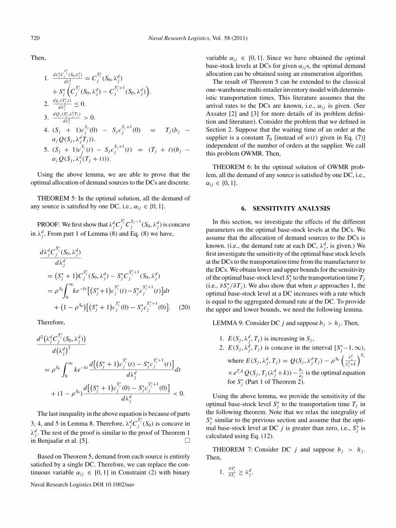
Then,

1.dλd

j CS∗j

j (S0,λdj )

dλdj

= CS∗

j

j (S0, λdj )

+ S∗j

(C

S∗j

j (S0, λdj ) − C

S∗j +1

j (S0, λdj ))

.

2.dgj (S

∗j ,t)

dλdj

≤ 0.

3.dQj (S

∗j ,λd

j Tj )

dλdj

> 0.

4. (Sj + 1)cSj

j (0) − SjcSj +1j (0) = Tj (bj −

ajQ(Sj , λdj Tj )).

5. (Sj + 1)cSj

j (t) − SjcSj +1j (t) = (Tj + t)(bj −

ajQ(Sj , λdj (Tj + t))).

Using the above lemma, we are able to prove that theoptimal allocation of demand sources to the DCs are discrete.

THEOREM 5: In the optimal solution, all the demand ofany source is satisfied by one DC, i.e., αij ∈ {0, 1}.

PROOF: We first show that λdj C

S∗j

j CSj −1j (S0, λd

j ) is concavein λd

j . From part 1 of Lemma (8) and Eq. (8) we have,

dλdj C

S∗j

j (S0, λdj )

dλdj

= (S∗

j + 1)C

S∗j

j (S0, λdj ) − S∗

j CS∗

j +1j (S0, λd

j )

= ρS0

∫ ∞

0ke−kt

[(S∗

j +1)cS∗

j

j (t)−S∗j c

S∗j +1

j (t)]dt

+ (1 − ρS0

)[(S∗

j + 1)cS∗

j

j (0) − S∗j c

S∗j +1

j (0)]. (20)

Therefore,

d2(λd

j CS∗

j

j (S0, λdj ))

d(λd

j

)2

= ρS0

∫ ∞

0ke−kt

d[(

S∗j + 1

)cS∗

j

j (t) − S∗j c

S∗j +1

j (t)]

dλdj

dt

+ (1 − ρS0)d[(

S∗j + 1

)cS∗

j

j (0) − S∗j c

S∗j +1

j (0)]

dλdj

< 0.

The last inequality in the above equation is because of parts

3, 4, and 5 in Lemma 8. Therefore, λdj C

S∗j

j (S0) is concave inλd

j . The rest of the proof is similar to the proof of Theorem 1in Benjaafar et al. [5]. �

Based on Theorem 5, demand from each source is entirelysatisfied by a single DC. Therefore, we can replace the con-tinuous variable αij ∈ [0, 1] in Constraint (2) with binary

variable αij ∈ {0, 1}. Since we have obtained the optimalbase-stock levels at DCs for given αij s, the optimal demandallocation can be obtained using an enumeration algorithm.

The result of Theorem 5 can be extended to the classicalone-warehouse multi-retailer inventory model with determin-istic transportation times. This literature assumes that thearrival rates to the DCs are known, i.e., αij is given. (SeeAxsater [2] and [3] for more details of its problem defini-tion and literature). Consider the problem that we defined inSection 2. Suppose that the waiting time of an order at thesupplier is a constant T0 [instead of w(t) given in Eq. (7)]independent of the number of orders at the supplier. We callthis problem OWMR. Then,

THEOREM 6: In the optimal solution of OWMR prob-lem, all the demand of any source is satisfied by one DC, i.e.,αij ∈ {0, 1}.

6. SENSITIVITY ANALYSIS

In this section, we investigate the effects of the differentparameters on the optimal base-stock levels at the DCs. Weassume that the allocation of demand sources to the DCs isknown. (i.e., the demand rate at each DC, λd

j , is given.) Wefirst investigate the sensitivity of the optimal base stock levelsat the DCs to the transportation time from the manufacturer tothe DCs. We obtain lower and upper bounds for the sensitivityof the optimal base-stock levelS∗

j to the transportation timeTj

(i.e., ∂S∗j /∂Tj ). We also show that when ρ approaches 1, the

optimal base-stock level at a DC increases with a rate whichis equal to the aggregated demand rate at the DC. To providethe upper and lower bounds, we need the following lemma.

LEMMA 9: Consider DC j and suppose bj > hj . Then,

1. E(Sj , λdj , Tj ) is increasing in Sj ,

2. E(Sj , λdj , Tj ) is concave in the interval [S∗

j −1, ∞),

where E(Sj , λdj , Tj ) = Q(Sj , λd

j Tj ) − ρS0

(λd

j

λdj +k

)Sj

×eTj kQ(Sj , Tj (λdj +k))− bj

ajis the optimal equation

for S∗j (Part 1 of Theorem 2).

Using the above lemma, we provide the sensitivity of theoptimal base-stock level S∗

j to the transportation time Tj inthe following theorem. Note that we relax the integrality ofS∗

j similar to the previous section and assume that the opti-mal base-stock level at DC j is greater than zero, i.e., S∗

j iscalculated using Eq. (12).

THEOREM 7: Consider DC j and suppose bj > hj .Then,

1.∂S∗

j

∂Tj≥ λd

j .



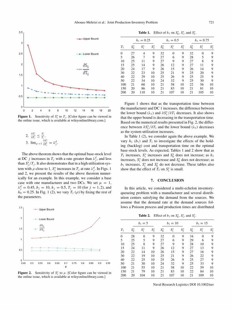
Figure 1. Sensitivity of S∗1 to Tj . [Color figure can be viewed in

the online issue, which is available at wileyonlinelibrary.com.]

2.∂S∗

j

∂Tj≤ S∗

j

Tj.

3. limρ→1∂S∗

j

∂Tj= λd

j .

The above theorem shows that the optimal base-stock levelat DC j increases in Tj with a rate greater than λd

j , and lessthan S∗

j /Tj . It also demonstrates that in a high utilization sys-tem with ρ close to 1, S∗

j increases in Tj at rate λdj . In Figs. 1

and 2, we present the results of the above theorem numer-ically for an example. In this example, we consider a basecase with one manufacturer and two DCs. We set µ = 1,λd

j = 0.45, bj = 10, hj = 0.5, Tj = 10 (for j = 1, 2), andh0 = 0.25. In Fig. 1 (2), we vary T1 (ρ) by fixing the rest ofthe parameters.

Figure 2. Sensitivity of S∗1 to ρ. [Color figure can be viewed in

the online issue, which is available at wileyonlinelibrary.com.]

Table 1. Effect of h1 on S∗0 , S∗

1 , and S∗2 .

h1 = 0.25 h1 = 0.5 h1 = 0.75

T1 S∗0 S∗

1 S∗2 S∗

0 S∗1 S∗

2 S∗0 S∗

1 S∗2

0 27 4 9 32 0 9 32 0 95 26 7 9 27 6 9 28 5 910 25 11 9 27 9 9 27 8 915 25 14 9 26 12 9 27 11 920 24 17 9 26 15 9 26 14 930 22 23 10 25 21 9 25 20 940 22 29 10 25 26 9 25 25 950 22 34 10 24 32 9 25 30 9100 21 60 10 21 58 10 22 56 10150 20 86 10 21 83 10 21 81 10200 20 110 10 21 107 10 21 105 10

Figure 1 shows that as the transportation time betweenthe manufacturer and DC 1 increases, the difference betweenthe lower bound (λ1) and ∂S∗

1/∂T1 decreases. It also showsthat the upper bound is decreasing in the transportation time.Based on the numerical results presented in Fig. 2, the differ-ence between ∂S∗

1/∂T1 and the lower bound (λ1) decreasesas the system utilization increases.

In Table 1 (2), we consider again the above example. Wevary h1 (b1) and T1 to investigate the effects of the hold-ing (backlog) cost and transportation time on the optimalbase-stock levels. As expected, Tables 1 and 2 show that asT1 increases, S∗

1 increases and S∗0 does not increase; as h1

increases, S∗1 does not increase and S∗

0 does not decrease; asb1 increases, S∗

1 and S∗0 do not decrease. These tables also

show that the effect of T1 on S∗2 is small.

7. CONCLUSION

In this article, we considered a multi-echelon inventory-queueing problem with a manufacturer and several distrib-ution centers satisfying the demand from the sources. Weassume that the demand rate at the demand sources fol-lows a Poisson process and production times are distributed

Table 2. Effect of b1 on S∗0 , S∗

1 , and S∗2 .

b1 = 5 b1 = 10 b1 = 15

T1 S∗0 S∗

1 S∗2 S∗

0 S∗1 S∗

2 S∗0 S∗

1 S∗2

0 28 0 9 32 0 9 34 0 95 25 5 9 27 6 9 29 6 910 25 8 9 27 9 9 28 10 915 24 11 9 26 12 9 27 13 920 22 14 10 26 15 9 27 16 930 22 19 10 25 21 9 26 22 940 22 25 10 25 26 9 25 27 950 21 30 10 24 32 9 25 33 9100 21 55 10 21 58 10 22 59 10150 21 79 10 21 83 10 22 84 10200 20 104 10 21 107 10 21 109 10



exponentially. We formulated the problem using the knownunit-flow method observed by Axsater [3]. To simplify theobjective function and obtain the structural properties ofthe cost functions, we defined the Normalized IncompleteGamma Function (NIGF) and demonstrated several interest-ing properties of NIGF. Using NIGF, we obtained the optimalbase-stock levels at the DCs and provided several conditionsunder which a DC prefers to keep some inventory to decreasethe backlog cost. We proved that the optimal demand allo-cation is always discrete and the total cost is convex in thewarehouse’s base-stock level. We also proved that in a sys-tem with high utilization (with a ρ close to one), the optimalbase-stock level at a DC increases in transportation time withthe demand rate arriving to the DC.

There are several potential directions for future research:(i) extend the problem to the case where inventories at theDCs are managed using the (r , Q) policy. This means thatDCs place orders in batches to the warehouse. (ii) considera priority policy at the manufacturer since DCs have differ-ent backlog costs. (iii) assume that backlog costs vary bythe demand sources. Therefore, the backlog costs at a DCdepends on the demand sources and it might be optimal toration the inventory at the DCs. This means that a DC mightdecrease its cost by keeping some inventory for the demandsources with high backlog costs even when there are somedemand from the sources with low backlog costs.

APPENDIX A

PROOF OF LEMMA 1: If the base stock level of a DC is zero, we cancalculate the cost C0

j (S0) using Eq. (8) as follows:

C0j (S0, λd

j ) = ρS0

∫ ∞

0ke−kt c0

j (t)dt + (1 − ρS0 )c0j (0).

Using (5) we get,

C0j (S0, λd

j ) = ρS0

∫ ∞

0ke−kt bj (Tj + t)dt + (1 − ρS0 )bj (Tj )

= ρS0

[bj Tj

∫ ∞

0ke−kt dt + bj

∫ ∞

0ke−kt tdt

]+ (1 − ρS0 )bj Tj = ρS0

bj

k+ bj Tj .

PROOF OF LEMMA 2:

1. Gj (Sj , t) =∫ t

0gj (Sj , s)ds =

∫ t

0

(λd

j

)Sj sSj −1e−λd

js

(Sj − 1)! ds

= (λd

j

)Sj

∫ t

0

sSj −1e−λd

js

(Sj − 1)! ds.

Let define R = λdj s. Then,

Gj (Sj , t) = (λd

j

)Sj

∫ λdjt

0

RSj −1e−R(λd

j

)−1(λd

j

)Sj −1(Sj − 1)!

dR

=∫ λd

jt

0 RSj −1e−RdR

(Sj − 1)! = 1 − Q(Sj , λdj t). (A1)

2. Based on the definition of Q(l, Y (x)) we have,

Q(l, Y (x)) =∫∞Y (x)

e−yyl−1dy

(l − 1)! .

Then, by taking the derivative with respect to x we get,

dQ(l, Y (x))

dx= − dY (x)

dx

e−Y (x)(Y (x))l−1

(l − 1)! .

3. Based on the definition of Q(l, Y (x)) and using the integration by partswe have,

Q(l + 1, ax) =∫∞ax

e−yyldy

(l)!= −e−yyl

(l)!∣∣∣∣y = ∞y = ax

+∫∞ax

le−yyl−1dy

(l)!

= e−ax(ax)l

(l)! +∫∞ax

e−yyl−1dy

(l − 1)!= e−ax(ax)l

(l)! + Q(l, ax). (A2)

4. Based on part 3 we have,

Q(l + 1, ax) − Q(l, ax) = e−ax(ax)l

(l)! = 1

a

(a

e−ax(ax)l

(l)!)

Then, using part 2 with Y (x) = ax we have,

Q(l + 1, ax) − Q(l, ax) = − 1

a

dQ(l + 1, ax)

dx.

PROOF OF LEMMA 3:

1. Using integration by parts and based on part 2 of Lemma 2,∫ ∞

0ke−ktQ(l, a′(b′ + t))dt

= −e−ktQ(l, a′(b′ + t))

∣∣∣∣t = ∞t = 0

−∫ ∞

0e−kt

(a′

(l − 1)! e−a′(b′+t)(a′(b′ + t))l−1

)dt

= Q(l, a′b′) − a′

(l − 1)!×∫ ∞

0e−kt (e−a′(b′+t)(a′(b′ + t))l−1)dt (A3)

Let define y = b′ + t . Then,∫ ∞


= Q(l, a′b′) − a′

(l − 1)!∫ ∞

b′e−a′y−k(y−b′)((a′y)l−1)dy

= Q(l, a′b′) − (a′)lekb′

(l − 1)!∫ ∞

b′e−y(a′+k)yl−1dy



Let define p = y(a′ + k). Then,∫ ∞


= Q(l, a′b′) − (a′)lekb′

(l − 1)!∫ ∞

b′(a′+k)

e−p

(p

a′ + k

)l−1

(a′ + k)−1dp

= Q(l, a′b′) −(

a′

a′ + k

)l

ekb′Q(l, b′(a′ + k)). (A4)

2. Using integration by parts and bases on part 2 of Lemma 2∫ ∞

0ke−ktQ(l, a′(b′ + t))(b′ + t)dt

= b′Q(l, a′b′) +∫ ∞

0e−ktQ(l, a′(b′ + t))dt

−∫ ∞

0e−kt e−a′(b′+t)(a′(b′ + t))l

(l − 1)! dt .

Based on part 1 we get,∫ ∞

0ke−ktQ(l, a′(b′ + t))(b′ + t)dt = b′Q(l, a′b′)

+ 1

k

(Q(l, a′b′) −

(a′

a′ + k

)l

eb′kQ(l, b′(a′ + k))

)

− l

a′

(a′

(l)!∫ ∞

0e−kt e−a′(b′+t)(a′(b′ + t))l

)dt . (A5)

The third term in Eq. (A5) is very similar to the second term in (A3).Therefore, using the second term of (A4) we get,∫ ∞

0ke−ktQ(l, a′(b′ + t))(b′ + t)dt = b′Q(l, a′b′)

+ 1

k

(Q(l, a′b′) −

(a′

a′ + k

)l

eb′kQ(l, b′(a′ + k))

)

− l

a′

((a′

a′ + k

)l+1

eb′kQ(l + 1, b′(a′ + k))

).

PROOF OF LEMMA 4:

1. Based on Eq. (6) and part 1 of Lemma 2, we have,

cSj

j (t) = (1 − Gj (Sj + 1, Tj + t))(aj )Sj

λdj

− (1 − Gj (Sj , Tj + t))(aj )(Tj + t) + bj

(Tj + t − Sj

λdj

)

= Q(Sj + 1, λd

j (Tj + t))(aj )

Sj

λdj

− Q(Sj , λd

j (Tj + t))(aj )(Tj + t) + bj

(Tj + t − Sj

λdj

)(A6)

Therefore,

cSj

j (0) = (aj )

(Sj

λdj

Q(Sj + 1, λdj Tj ) − TjQ(Sj , λd

j Tj )

)+ bj Tj − bj Sj

λdj

.

(A7)

2. Based on part 1 we have,

cSj

j (0) − cSj −1j (0)

= aj

(Sj

λdj

[Q(Sj + 1, λd

j Tj

)− Q(Sj , λd

j Tj

)]+ 1

λdj

Q(Sj , λd

j Tj

))

− aj

(Tj

[Q(Sj , λd

j Tj ) − Q(Sj − 1, λd

j Tj

)])− bj

λdj

.

Using part 3 of Lemma 2 we get,

cSj

j (0) − cSj −1j (0) = aj

Sj

λdj

(λdj Tj

)Sj e−λd

jTj

Sj !

+ 1

λdj

Q(Sj , λd

j Tj

)

− Tj

(λdj Tj

)Sj −1e−λd

jTj

(Sj − 1)!

− bj

λdj

= aj

λdj

Q(Sj , λdj Tj ) − bj

λdj

.

PROOF OF LEMMA 5:

1. Based on Eq. (A6),

fj (Sj ) =∫ ∞

0ke−kt

[Q(Sj + 1, λd

j (Tj + t))(aj )Sj

λdj

− Q(Sj , λd

j (Tj + t))(aj )(Tj + t)

]dt

+∫ ∞

0ke−kt

[bj

(Tj + t − Sj

λdj

)]dt

= aj

(Sj

λdj

∫ ∞

0ke−ktQ

(Sj + 1, λd

j (Tj + t))dt

−∫ ∞

0ke−ktQ

(Sj , λd

j (Tj + t))(Tj + t)dt

)+ bj

(Tj − Sj

λdj

+ 1

k

). (A8)

Then, based on Lemma 3,

fj (Sj ) = aj

[Sj

λdj

Q(Sj + 1, λd

j Tj

)− TjQ(Sj , λd

j Tj

)− 1

k

(Q(Sj , λd

j Tj

)− δj (Sj ))]+ bj

(Tj − Sj

λdj

+ 1

k

). (A9)

2. By definition,

fj (Sj ) − fj (Sj − 1) =∫ ∞

0ke−kt

(cSj

j (t) − cSj −1j (t)

)dt . (A10)

Since the arrivals are Poisson distributed, we have (Axsatet 1990),

dcSj

j (t)

dt= −λd

j

(cSj

j (t) − cSj −1j (t)

). (A11)



By substituting (A11) in (A10) and integration by parts we get,

fj (Sj ) − fj (Sj − 1)

=∫ ∞

0ke−kt

−1

λdj

dcSj

j (t)

dt

dt

= 1

λdj

(−ke−kt c

Sj

j (t)

∣∣∣∣t = ∞t = 0

− k

∫ ∞

0ke−kt c

Sj

j (t)dt

)= k

λdj

(cSj

j (0) − fj (Sj ))

. (A12)

By substituting part 1 of Lemma 4 and (A9) in (A12) we get,

fj (Sj ) − fj (Sj − 1) = k

λdj

(aj

k

(Q(Sj , λd

j Tj

)− δj (Sj ))− bj

k

)= 1

λdj

[aj

(Q(Sj , λd

j Tj ) − δj (Sj ))− bj

].

PROOF OF LEMMA 6: From Eq. (8) we have,

CSj

j

(S0, λd

j

) = ρS0

∫ ∞

0w(t)c

Sj

j (t)dt + (1 − ρS0 )cSj

j (0). (A13)

Similar to the proof of part 2 of Lemma 4 we can show that

cSj

j (t) − cSj −1j (t) = aj

λdj

Q(Sj , λd

j (Tj + t))− bj

λdj

.

Then,

(cSj +1j (t) − c

Sj

j (t))− (

cSj

j (t) − cSj −1j (t)

)= aj

λdj

(Q(Sj + 1, λd

j (Tj + t))− Q

(Sj , λd

j (Tj + t)))

. (A14)

Using part 3 of Lemma 2, we can rewrite the above equation as,

(cSj +1j (t) − c

Sj

j (t))− (

cSj

j (t) − cSj −1j (t)

)= aj

λdj

e−λd

j(Tj +t)(

λdj (Tj + t)

)Sj

Sj !

> 0. (A15)

Therefore, cSj

j (t) is convex in Sj .By substituting t = 0 in the above equation, we get

(cSj +1j (0) − c

Sj

j (0))− (

cSj

j (0) − cSj −1j (0)

)> 0. (A16)

and therefore cSj

j (0) is convex in Sj . Since cSj

j (t) and cSj

j (0) are convex,

from (A13) CSj

j (S0, λdj ) is convex in Sj .

PROOF OF THEOREM 3: From Eq. (12) it is straightforward to see thatS∗

j is decreasing in S0. Therefore, we can obtain a lower bound for the opti-mal base-stock at DC j by substituting S0 = ∞ in Eq. (12) which resultsin,

Q(SL

j , λdj Tj

) = bj

hj + bj

. (A17)

Q(Sj , λdj Tj ) is decreasing in λd

j Tj based on (9) and increasing in Sj since

Q(SL

j , λdj Tj

) =Sj −1∑i=0

(λd

j Tj

)ie−λd

jTj

i! .

Then, SLj increases if λd

j Tj increases since the right hand side of Eq. (A17)is a constant. This means that if we replace Sj by 1 in (A17) we get a sufficientcondition under which the optimal base-stock at DC j is positive.

Q(1, λd

j Tj

) = bj

hj + bj

⇒∫ ∞

λdjTj

e−ydy

= bj

hj + bj

⇒ e−λd

jTj = bj

hj + bj

⇒ λdj Tj = − ln

(bj

hj + bj

).

Therefore, if λdj Tj ≥ − ln

(bj

hj +bj

), the optimal base-stock level at DC j

is positive.

PROOF OF LEMMA 7: We first show that

CSj

j

(S0, λd

j

) = ρS0(C

Sj

j (0, λdj ) − C

Sj

j (∞, λdj ))+ C

Sj

j (∞, λdj ). (A18)

From (8)

CSj

j

(S0, λd

j

) = ρS0

∫ ∞

0ke−kt c

Sj

j (t)dt + (1 − ρS0 )cSj

j (0)

⇒ CSj

j

(S0, λd

j

)− ρCSj

j (S0 − 1, λdj ) = (1 − ρ)c

Sj

j (0).

Therefore,

CSj

j

(S0, λd

j

) = ρS0(C

Sj

j (0, λdj ) − C

Sj

j (∞, λdj ))+ C

Sj

j (∞, λdj ).

From the above equation, it is obvious that CSj

j (S0, λdj ) is convex in S0.

The manufacturer holding cost, C0(S0), which is given in Eq. (15) is alsoconvex in S0. Therefore, the total cost of the system, Z,

Z =m∑

j=1

λdj C

Sj

j

(S0, λd

j

)+m∑

j=1

n∑i=1

αij cij λi + C0(S0)

is convex in the base-stock level of the warehouse, S0.

PROOF OF THEOREM 4: Here, we relax the integrality of S0. SinceU(S0, S1, . . . , Sm) is convex in S0 based on Lemma 7, an integer upperbound for the relaxed case is also an upper bound for S∗

0 .To obtain an upper bound for the optimal base-stock level at the

manufacturer, we consider U(S0, S1, . . . , Sm). From (8) we have

CSj

j

(S0, λd

j

) = ρS0 fj (Sj ) + (1 − ρS0 )cSj

j (0).

Therefore using (15),

∂U(S0, S1, . . . , Sm)

∂S0

= ρS0 (ln ρ)

m∑j=1

λdj

(fj (Sj ) − c

Sj

j (0))+ h0 + ρS0+1(ln ρ)

1 − ρh0.



From (A12) we have,

fj (Sj ) − fj (Sj − 1) = k

λdj

(cSj

j (0) − fj (Sj )). (A19)

Also, from part 2 of Lemma 5 we have,

fj (Sj ) − fj (Sj − 1)

= 1

λdj

aj

Q(Sj , λd

j Tj

)− ekTj

(λd

j

λdj + k

)Sj

Q(Sj , Tj

(λd

j + k)− bj

.

(A20)

Therefore (substituting k = µ(1 − ρ) in the second expression below),

∂U(S0, S1, . . . , Sm)

∂S0= ρS0 (ln ρ)

m∑j=1

−λdj

k

aj

Q(Sj , λdj Tj )

−ekTj

(λd

j

λdj + k

)Sj

Q(Sj , Tj

(λd

j + k)− bj

+ h0 + ρS0+1(ln ρ)

1 − ρh0

= ρS0 (ln ρ)

1 − ρ

m∑j=1

λdj

µ

bj − aj

Q(Sj , λdj Tj )

−ekTj

(λd

j

λdj + k

)Sj

Q(Sj , Tj (λdj + k)

+ ρS0 (ln ρ)

1 − ρ[ρh0] + h0.

SinceSu0 is the optimal solution of minimizingU (S0, S1(∞), . . . , Sm(∞)),

then it is the solution of

∂U(S0, S1(∞), . . . , Sm(∞))

∂S0= 0.

Based on part 1 of Theorem 2 we know that S∗j is the solution of the

following equation,

Q(Sj , λd

j Tj

)− ρS0

(λd

j

λdj + k

)Sj

eTj kQ(Sj , Tj

(λd

j + k))− bj

aj

= 0.

(A21)

By substituting S0 = ∞ in (A21) we get,

Q(Sj , λd

j Tj

) = bj

aj

. (A22)

Let Sj denote the solution of the above equation, i.e.,

Q(Sj , λd

j Tj

) = bj

aj

. (A23)

Therefore,

∂U(S0, S1(∞), . . . , Sm(∞))

∂S0

= ρS0 (ln ρ)

1 − ρ

m∑j=1

λdj

µaj e

kTj

(λd

j

λdj + k

)Sj

Q(Sj , Tj (λdj + k) + ρh0

+ h0

= ρS0 (ln ρ)

1 − ρ[v + ρh0] + h0.

From FOC,

ρSu0 = h0(ρ − 1)

(ln ρ)[v + ρh0] ⇒ Su0 =

⌈ln(

(ρ−1)h0(ln ρ)[v+ρh0] )

ln ρ

⌉.

PROOF OF LEMMA 8:

1. Using (8),

λdj C

S∗j

j (S0, λdj ) = ρS0

∫ ∞

0ke−kt λd

j cS∗j

j (t)dt + (1 − ρS0 )λdj c

S∗j

j (0). (A24)

In Eq. (A24) λdj c

Sj

j (t) and λdj c

Sj

j (0) are the terms which depend on λdj .

Let us first consider Q(S∗j , λd

j Tj ). Then, using implicit differentiation

dQ(S∗

j , λdj Tj

)dλd

j

= dQ(Sj , λd

j Tj

)dλd

j

∣∣∣Sj =S∗j

+ dS∗j

dλdj

dQ(Sj , λd

j Tj

)dSj

∣∣∣Sj =S∗j

.

(A25)

Now we consider λdj c

Sj

j (t). From (A6)

dλdj c

S∗j

j (t)

dλdj

= aj

(dS∗

j

dλdj

Q(S∗

j + 1, λdj (Tj + t)

)+ S∗j

dQ(S∗

j + 1, λdj (Tj + t)

)dλd

j

)

− aj

((Tj + t)Q

(S∗

j , λdj (Tj + t)

)+ (Tj + t)λdj

dQ(S∗

j , λdj (Tj + t)

)dλd

j

)

+ bj (Tj + t) − bj

dS∗j

dλdj

.

Using (A25) we get,

dλdj c

S∗j

j (t)

dλdj

= aj

(dS∗

j

dλdj

Q(S∗

j + 1, λdj (Tj + t)

))

+ aj

(S∗

j

[dQ

(Sj + 1, λd

j Tj

)dλd

j

∣∣∣Sj =S∗j

+ dS∗j

dλdj

dQ(Sj + 1, λd

j Tj

)dSj

∣∣∣Sj =S∗j

])− aj

((Tj + t)Q

(S∗

j , λdj (Tj + t)

))+ aj

((Tj + t)λd

j

[dQ

(Sj , λd

j Tj

)dλd

j

∣∣∣Sj =S∗j

+ dS∗j

dλdj

dQ(Sj , λd

j Tj

)dSj

∣∣∣Sj =S∗j

])

+ bj (Tj + t) − bj

dS∗j

dλdj

.

dλdj c

S∗j

j (t)

dλdj

= dS∗j

dλdj

aj

(Q(S∗

j + 1, λdj (Tj + t)

)+ S∗j

dQ(Sj + 1, λd

j Tj

)dSj

∣∣∣Sj =S∗j

)

− dS∗j

dλdj

aj

((Tj + t)λd

j

dQ(Sj , λd

j Tj

)dSj

∣∣∣Sj =S∗j

− bj

)

+ aj

(S∗

j

dQ(Sj + 1, λd

j Tj

)dλd

j

∣∣∣Sj =S∗j

)

− aj

[(Tj + t)Q

(S∗

j , λdj (Tj + t)

)+ (Tj + t)λdj

dQ(Sj , λd

j Tj

)dλd

j

∣∣∣Sj =S∗j

]+ bj (Tj + t).



Based on the above equation we have,

dλdj c

S∗j

j (t)

dλdj

= dS∗j

dλdj

dλdj c

Sj

j (t)

dS∗j

∣∣∣Sj =S∗j

+ dλdj c

Sj

j (t)

dλdj

∣∣∣Sj =S∗j

. (A26)

Now we considerdλd

jC

S∗j

j(S0)

dλdj

.

dλdj C

S∗j

j (S0, λdj )

dλdj

= ρS0

∫ ∞

0ke−kt

dλdj c

S∗j

j (t)

dλdj

dt + (1 − ρS0 )dλd

j cS∗j

j (0)

dλdj

.

Using (A26) we have,

dλdj C

S∗j

j (S0, λdj )

dλdj

= ρS0

∫ ∞

0ke−kt

dS∗j

dλdj

dλdj c

Sj

j (t)

dS∗j

∣∣∣Sj =S∗j

+ dλdj c

Sj

j (t)

dλdj

∣∣∣Sj =S∗j

dt

+ (1 − ρS0 )

dS∗j

dλdj

dλdj c

Sj

j (0)

dS∗j

∣∣∣Sj =S∗j

+ dλdj c

Sj

j (0)

dλdj

∣∣∣Sj =S∗j

= dS∗

j

dλdj

dλdj C

Sj

j (S0, λdj )

dS∗j

∣∣∣Sj =S∗j

+ dλdj C

Sj

j (S0, λdj )

dλdj

∣∣∣Sj =S∗j

.

Since S∗j is the optimal solution of minimizing λd

j CSj

j (S0, λdj ), we get,

dλdj C

S∗j

j (S0, λdj )

dλdj

= dλdj C

Sj

j (S0, λdj )

dλdj

∣∣∣Sj =S∗j

. (A27)

Now we considerdC

Sjj

(S0,λdj)

dλdj

.

dCSj

j (S0, λdj )

dλdj

= ρS0

∫ ∞

0ke−kt

dcSj

j (t)

dλdj

dt + (1 − ρS0 )dc

Sj

j (0)

dλdj

. (A28)

As we see in (A28), CSj

j (S0, λdj ) is a function of λd

j only through cSj

j (t)

and cSj

j (0).We first find the derivative of cSj

j (t) with respect to λdj . From (5)

we have,

dcSj

j (t)

dλdj

= bj

∫ Tj +t

0

dgj (Sj , s)

dλdj

(Tj +t −s)ds+hj

∫ ∞

Tj +t

dgj (Sj , s)

dλdj

(s−Tj −t)ds.

(A29)

Also, from (4) we have,

dgj (Sj , t)

dλdj

=(

Sj

λdj

− t

)gj (Sj , t), (A30)

tgj (Sj , t) = Sj

λdj

gj (Sj + 1, t). (A31)

By substituting (A30) in (A29) we get,

dcSj

j (t)

dλdj

= bj

∫ Tj +t

0

(Sj

λdj

− s

)gj (Sj , s)(Tj + t − s)ds

+ hj

∫ ∞

Tj +t

(Sj

λdj

− s

)gj (Sj , s)(s − Tj − t)ds

= Sj

λdj

(bj

∫ Tj +t

0gj (Sj , s)(Tj + t − s)ds

+hj

∫ ∞

Tj +t

gj (Sj , s)(s − Tj − t)ds

)

−(

bj

∫ Tj +t

0sgj (Sj , s)(Tj + t − s)ds

+hj

∫ ∞

Tj +t

sgj (Sj , s)(s − Tj − t)ds

). (A32)


dcSj

j (t)

dλdj

= Sj

λdj

cSj

j (t) − Sj

λdj

cSj +1j (t) = Sj

λdj

(cSj

j (t) − cSj +1j (t)

). (A33)


dCSj

j

(S0, λd

j

)dλd

j

= ρS0

∫ ∞

0ke−kt Sj

λdj

(cSj

j (t) − cSj +1j (t)

)dt

+ (1 − ρS0 )Sj

λdj

(cSj

j (0) − cSj +1j (0)

)= Sj

λdj

(C

Sj

j (S0, λdj ) − C

Sj +1j (S0, λd

j )). (A34)

Therefore,

dλdj C

Sj

j

(S0, λd

j

)dλd

j

= CSj

j

(S0, λd

j

)+ Sj

(C

Sj

j

(S0, λd

j

)− CSj +1j (S0)

).

Using (A27) we get,

dλdj C

S∗j

j (S0, λdj )

dλdj

= CS∗j

j (S0) + S∗j

(C

S∗j

j (S0, λdj ) − C

S∗j+1

j (S0, λdj )).

(A35)

2. The proof is by contradiction. Supposedgj (S∗

j,t)

dλdj

> 0. From (A29) it is

obvious that ifdgj (S∗

j,t)

dλdj

> 0, thendc

S∗j

j(t)

dλdj

> 0, which results indC

S∗j

j(S0)

dλdj

> 0

based on (A28). But, from (A34) we get,

dCS∗j

j (S0, λdj )

dλdj

= S∗j

λdj

(C

S∗j

j (S0, λdj ) − C

S∗j+1

j (S0, λdj )) ≤ 0.

The above inequality is because of the fact that S∗j is the optimal solution

of λdj C

Sj

j (S0, λdj ) and C

Sj

j (S0, λdj ) is a convex function in Sj . This inequality

contradicts the fact thatdgj (S∗

j,t)

dλdj

> 0; hence, we must havedgj (S∗

j,t)

dλdj

≤ 0.



3. From part 2 and the fact that QS∗j

j (S∗j , λd

j Tj ) = 1 − ∫ t

0 gj (S∗j , s)ds, we

get the desired result.4. From (A7),

(Sj + 1)cSj

j (0) − Sj cSj +1j (0) = (Sj + 1)

×[aj

(Sj

λdj

Q(Sj + 1, λd

j Tj

)− TjQ(Sj , λd

j Tj

))+ bj Tj − bj Sj

λdj

]

− Sj

[aj

((Sj + 1)

λdj

Q(Sj + 2, λd

j Tj

)− TjQ(Sj + 1, λd

j Tj

))]

− Sj

[bj Tj − bj (Sj + 1)

λdj

]

= aj

(Sj + 1)Sj

λdj

[Q(Sj + 1, λd

j Tj

)− Q(Sj + 2, λd

j Tj

)]− aj Tj

[(Sj + 1)Q

(Sj , λd

j Tj

)− SjQ(Sj + 1, λd

j Tj

)]+ bj Tj .

Using part 3 of Lemma 2 we get,

(Sj + 1)cSj

j (0) − Sj cSj +1j (0)

= aj

(Sj + 1)Sj

λdj

−e−λd

jTj(λd

j Tj

)Sj +1

(Sj + 1)!

− aj Tj

Q(Sj , λd

j Tj

)− Sj

e−λd

jTj(λd

j Tj

)Sj

Sj !

+ bj Tj

= aj

−Tj

e−λd

jTj(λd

j Tj

)Sj

(Sj − 1)! + Tj

e−λd

jTj(λd

j Tj

)Sj

(Sj − 1)!

− aj TjQ(Sj , λd

j Tj ) + bj Tj

= Tj

(bj − ajQ

(Sj , λd

j Tj

)).

5. Similar to part 3 we get,

(Sj + 1)cSj

j (t) − Sj cSj +1j (t) = (Tj + t)

(bj − ajQ

(Sj , λd

j (Tj + t)))

.

(A36)

PROOF OF THEOREM 6: Let CSj

j (S0, λdj ) denote the expected inven-

tory carrying and backlog costs at DC j incurred to fill a unit of demand inOWMR problem. Axsater [3] shows that

CSj

j

(S0, λd

j

) =∫ T0

0�(t)c

Sj

j (t)dt + (1 − G

S00

)cSj

j (0), (A37)

where

1 − GS00 =

S0−1∑k=0

λk0T

k0 e−λ0T0

k! ,

and

�(t) = λS00 (T0 − t)S0−1e−λ0(T0−t)

(S0 − 1)! ,

Since the bounds of the integral, �(t) and GS00 are independent of λj , we

have

dλdj C

S∗j

j (S0, λdj )

dλdj

=∫ T0

0�(t)

dλdj c

S∗j

j (t)

dλdj

dt + (1 − G

S00

)dλdj c

S∗j

j (0)

dλdj

=∫ T0

0�(t)

dS∗j

dλdj

dλdj c

Sj

j (t)

dSj

|Sj =S∗j

+ dλdj c

Sj

j (t)

dλdj

dt

+ (1 − G

S00

)dS∗j

dλdj

dλdj c

Sj

j (0)

dSj

|Sj =S∗j

+ dλdj c

Sj

j (0)

dλdj

=∫ T0

0�(t)

dλdj c

Sj

j (t)

dλdj

dt + (1 − G

S00

)dλdj c

Sj

j (0)

dλdj

.

(A38)

The last inequality holds becausedλd

jC

Sjj

(0)

dSj|Sj =S∗

j= 0. From Eq. (A33) we

have,

dcSj

j (t)

dλdj

= Sj

λdj

(cSj

j (t) − cSj +1j (t)

).

Therefore,

dλdj C

S∗j

j (S0, λdj )

dλdj

=∫ T0

0�(t)

cSj

j (t) + dcSj

j (t)

dλdj

dt

+ (1 − G

S00

)cSj

j (0) + dcSj

j (0)

dλdj

= (

S∗j + 1

)C

S∗j

j (S0) − S∗j C

S∗j+1

j (S0). (A39)

Noting that since Eq. (A39) is the same as Eq. (20), the rest of the proofis similar to the proof of Theorem 5.

PROOF OF LEMMA 9: Based on part 1 of Lemma 3 we have,

E(Sj , λd

j , Tj

)= Q

(Sj , λd

j Tj

)− ρS0

(λd

j

λdj + k

)Sj

eTj kQ(Sj , Tj

(λd

j + k))− bj

aj

= (1 − ρS0 )Q(Sj , λd

j Tj

)+ ρS0

∫ ∞

0ke−ktQ

(Sj , Tj

(λd

j + t))

dt .

(A40)

1. Q(Sj , λd

j Tj

)− Q(Sj − 1, λd

j Tj

) =(λd

j Tj

)Sj e−λd

jTj

Sj ! > 0.

Similarly,

Q(Sj , Tj

(λd

j + k))− Q

(Sj − 1, Tj

(λd

j + k))

=(Tj

(λd

j + k))Sj e

−Tj

(λdj+k)

Sj ! > 0.



Therefore, E(Sj , λdj , Tj ) is increasing in Sj .

2. Q(Sj + 1, λd

j Tj

)− 2Q(Sj , λd

j Tj

)+ Q(Sj − 1, λd

j Tj

)=(λd

j Tj

)Sj e−λd

jTj

Sj ! −(λd

j Tj

)Sj −1e−λd

jTj

(Sj − 1)!

=(λd

j Tj

)Sj −1e−λd

jTj

(Sj − 1)!

(λd

j Tj

Sj

− 1

). (A41)

Since bj ≥ hj , based on Eq. (12) S∗j should satisfy the following

inequality:

S∗j ≥ inf

{Sj : Q

(Sj , λd

j Tj

) ≥ 1

2

}. (A42)

Based on Theorem 1 in Adell and Jorda [1] and Eq. (A42), S∗j > λd

j Tj .Therefore based on Eq. (A41)

Q(Sj + 1, λd

j Tj

)− 2Q(Sj , λd

j Tj

)+ Q(Sj − 1, λd

j Tj

)> 0,

which means that E(Sj , λdj , Tj ) is concave in the interval [S∗

j − 1, ∞).

PROOF OF LEMMA 10:1. Using the implicit differentiation we have,

∂S∗j

∂Tj

= −∂E(Sj ,λd

j,Tj

)∂Tj

∂E(Sj ,λd

j,Tj

)∂Sj

∣∣∣Sj =S∗j

. (A43)

We first consider∂E(Sj ,λd

j,Tj )

∂Tj,

∂E(Sj , λd

j , Tj

)∂Tj

= ∂Q(Sj , λd

j Tj

)∂Tj

− kρS0

(λd

j

λdj + k

)Sj

eTj kQ(Sj , Tj

(λd

j + k))

− ρS0

(λd

j

λdj + k

)Sj

eTj k∂Q

(Sj , Tj

(λd

j + k))

∂Tj

. (A44)

Also, based on part 4 of Lemma 2 we have,

Q(Sj , Tjλ

dj

)− Q(Sj − 1, Tjλ

dj

) = − 1

λdj

∂Q(Sj , λd

j Tj

)∂Tj

. (A45)


∂E(Sj , λd

j , Tj

)∂Tj

= −λdj

(Q(Sj , Tjλ

dj

)− Q(Sj − 1, Tjλ

dj

))− kρS0

(λd

j

λdj + k

)Sj

eTj kQ(Sj , Tj

(λd

j + k))

+ ρS0

(λd

j

λdj + k

)Sj

eTj k(λd

j + k)(

Q(Sj , Tj

(λd

j + k))

− Q(Sj − 1, Tj

(λd

j + k)))

= −λdj

(Q(Sj , Tjλ

dj

)− Q(Sj − 1, Tjλ

dj

))+ ρS0

(λd

j

λdj + k

)Sj

eTj kλdj Q(Sj , Tj

(λd

j + k))

− ρS0

(λd

j

λdj + k

)Sj

eTj k(λd

j + k)Q(Sj − 1, Tj

(λd

j + k))

= −λdj

[Q(Sj , Tjλ

dj

)− Q(Sj − 1, Tjλ

dj

)−ρS0

(λd

j

λdj + k

)Sj

eTj kQ(Sj , Tj

(λd

j + k))

− λdj

ρS0

(λd

j

λdj + k

)Sj

eTj k

(λd

j + k

λdj

)Q(Sj − 1, Tj

(λd

j + k))

= −λdj

Q(Sj , Tjλ

dj

)− ρS0

(λd

j

λdj + k

)Sj

eTj kQ(Sj , Tj

(λd

j + k))

+ λdj

Q(Sj − 1, Tjλ

dj

)− ρS0

(λd

j

λdj + k

)Sj −1

× eTj kQ(Sj − 1, Tj

(λd

j + k))]

= −λdj

(E(Sj , λd

j , Tj

)− E(Sj − 1, λd

j , Tj

)). (A46)

Therefore, based on Eqs. (A43) and (A46) we have,

∂S∗j

∂Tj

= λdj

E(Sj , λd

j , Tj

)− E(Sj − 1, λd

j , Tj

)∂E(Sj ,λd

j,Tj

)∂Sj

∣∣∣Sj =S∗j

. (A47)

Based on Lemma (9), E(Sj , λdj , Tj ) is concave and increasing in the

interval [S∗j − 1, ∞). Therefore,

E(Sj , λd

j , Tj

)− E(Sj − 1, λd

j , Tj

) ≥ ∂E(Sj , λd

j , Tj

)∂Sj

∣∣∣Sj =S∗j

.

This implies that∂S∗

j

∂Tj≥ λd

j .

2. Based on Eq. (A47) and the fact that E(Sj , λdj , Tj ) is concave and

increasing in the interval [S∗j − 1, ∞) we have,

∂S∗j

∂Tj

= λdj

E(Sj , λd

j , Tj

)− E(Sj − 1, λd

j , Tj

)∂E(Sj ,λd

j,Tj

)∂Sj

≤ λdj

E(Sj , λd

j , Tj

)− E(Sj − 1, λd

j , Tj

)E(Sj + 1, λd

j , Tj

)− E(Sj , λd

j , Tj

) ∣∣∣Sj =S∗j

. (A48)



Now consider E(Sj , λdj , Tj ). Then,

E(Sj , λd

j , Tj

)− E(Sj − 1, λd

j , Tj

)= Q

(Sj , Tjλ

dj

)− Q(Sj − 1, Tjλ

dj

)− ρS0 eTj k

( λdj

λdj + k

)Sj

Q(Sj , Tj

(λd

j + k))

−(

λdj

λdj + k

)Sj −1

Q(Sj − 1, Tj

(λd

j + k))

= e−λd

jTj

(λdjTj

)Sj −1

(Sj − 1)! − ρS0 eTj k

(λd

j

λdj + k

)Sj −1

×[(

λdj

λdj + k

)Q(Sj , Tj

(λd

j + k))− Q

(Sj − 1, Tj

(λd

j + k))]

= e−λd

jTj

(λdjTj

)Sj −1

(Sj − 1)! − ρS0 eTj k

(λd

j

λdj + k

)Sj −1

×− k

λdj + k

Q(Sj , Tj

(λd

j + k))+ e

−(λdj+k)Tj

((λdj+k)Tj

)Sj −1

(Sj − 1)!

= e

−λdjTj

(λdjTj

)Sj −1

(Sj − 1)! + ρS0 eTj k

(λd

j

λdj + k

)Sj

× Q(Sj , Tj

(λd

j + k)) k

λdj

− ρS0e−λd

jTj

(λdjTj

)Sj −1

(Sj − 1)!

= (1 − ρS0 )e−λd

jTj

(λdjTj

)Sj −1

(Sj − 1)! + k

λdj

δj (Sj ). (A49)

Now we show that δj (Sj + 1)/δj (Sj ) > λdj Tj /Sj .

δj (Sj ) =(

λdj

λdj + k

)Sj

eTj kQ(Sj , Tj

(λd

j + k))

=∫ ∞

Tj (λdj+k)

e−ktλd

j

(Sj − 1)! e−λd

j(Tj +t)(

λdj (Tj + t)

)Sj −1dt . (A50)

Let define

Y (Sj ) = λdj

(Sj − 1)! e−λd

j(Tj +t)

(λdj (Tj + t))Sj −1.

Then,

Y (Sj + 1)

Y (Sj )= λd

j (Tj + t)

Sj

≥ λdj Tj

Sj

. (A51)

Therefore, based on Eqs. (A50) and (A51 ) we have

δj (Sj + 1)

δj (Sj )≥ λd

j Tj

Sj

. (A52)

Based on (A49) and (A52) we have,

E(Sj + 1, λd

j , Tj

)− E(Sj , λd

j , Tj

)≥ (1 − ρS0 )

e−λd

jTj

(λdjTj

)Sj

(Sj )! + λdj Tj

Sj

[k

λdj

δj (Sj )

]

= λdj Tj

Sj

(1 − ρS0 )e−λd

jTj

(λdjTj

)Sj −1

(Sj − 1)! + k

λdj

δj (Sj )

= λd

j Tj

Sj

(E(Sj , λd

j , Tj

)− E(Sj − 1, λd

j , Tj

)). (A53)

Therefore, based on Eqs. (A48) and (A53) we have,

∂S∗j

∂Tj

≤ λdj

E(Sj , λd

j , Tj

)− E(Sj − 1, λd

j , Tj

)E(Sj + 1, λd

j , Tj

)− E(Sj , λd

j , Tj

) ≤ Sj

Tj

∣∣∣Sj =S∗j

.

3. Based on Eq. (A49) we have,

E(Sj , λd

j , Tj

)− E(Sj − 1, λd

j , Tj

)= (1 − ρS0 )

e−λd

jTj

(λdjTj

)Sj −1

(Sj − 1)! + µ(1 − ρ)

λdj

δj (Sj ).

Since E(Sj , λdj , Tj ) is increasing and concave in Sj based on Lemma 9

in the interval [S∗j − 1, ∞), then

limρ→1

(E(Sj , λd

j , Tj

)− E(Sj − 1, λd

j , Tj

)) = 0. (A54)

Therefore, using (A54) and the fact that E(Sj , λdj , Tj ) is increasing and

concave in Sj in the interval [S∗j − 1, ∞), we get,

limρ→1

(E(Sj , λd

j , Tj

)− E(Sj − 1, λd

j , Tj

)) ∣∣∣Sj =S∗j

→ ∂E(Sj , λd

j , Tj

)∂Sj

∣∣∣Sj =S∗j

. (A55)

Thus, based on (A47) and (A55) we have,

limρ→1

∂S∗j

∂Tj

= limρ→1

λdj

E(Sj , λd

j , Tj

)− E(Sj − 1, λd

j , Tj

)∂E(Sj ,λd

j,Tj

)∂Sj

= λdj

∣∣∣Sj =S∗j

.

NOTATION

I set of demand sources.J set of distribution centers.

αij fraction of demand from source i assigned to DC j .λi demand rate of source i, ass a Poisson processes.



λdj = ∑

i∈I αijλi : Demand rate at DC j .λ0 = ∑

j∈J λdj : Demand rate at the manufacturer.

Sj base-stock level at DC j .S0 base-stock level at manufacturer.µ production rate at manufacturer.Tj transportation time between the manufacturer

and DC j .hj holding cost per unit and per unit time at DC j .h0 holding cost per unit and per unit time at

manufacturer.bj backlog cost per unit and per unit time at DC j .cij cost of satisfying an order of source i from

DC j .

CSj

j (S0, λdj ) expected inventory carrying and backlog costs

at DC j incurred to fill a unit of demand atDC j when its base-stock level is Sj and thebase-stock level of the manufacturer is S0.

C0(S0) average holding cost at the manufacturer.ρ = λ0/µ, system utilization.k = µ(1 − ρ).

aj hj + bj .

ACKNOWLEDGMENTS

The authors thank the editor, the associate editor, and thereferees for their valuable comments and suggestions. Thisarticle was supported by the NSERC grant of the secondauthor.

REFERENCES

[1] J.A. Adell and P. Jodra, The median of the Poisson distribution,Metrika 61 (2005), 337–346.

[2] S. Axsater, Inventory control, 2nd ed., Springer, New York,2006.

[3] S. Axsater, Simple solution procedures for a class of two-echelon inventory problems, Oper Res 38 (1990), 64–69.

[4] S. Benjaafar, M. Elhafsi, and F. de Vericourt, Demand allo-cation in multiple-product, multiple-facility make-to-stocksystems, Manage Sci 50 (2004), 1431–1448.

[5] S. Benjaafar, Y. Li, D. Xu, and S. Elhedli, Demand alloca-tion in systems with multiple inventory locations and multiple

demand sources, Manuf Serv Oper Manage 10 (2008),43–60.

[6] S. Benjaafar and D. Gupta, Workload allocation in multi-product, multi-facility production systems with setup times,IIE Trans 31 (1999), 339–352.

[7] O. Berman, K. Dmitry, and M.M. Tajbaksh, On the benefits ofrisk pooling in inventory management, Prod Oper Manage 20(2011), 55–71.

[8] J. Buzacott and J.G. Shanthikumar, Stochastic models ofmanufacturing systems, Prentice Hall, Englewood Cliffs, NJ,2003.

[9] A.J. Clark and H.E. Scarf, Optimal policies for a multi-echeloninventory problem, Manage Sci 6 (1960), 475–490.

[10] G.D. Eppen, Effects of centralization on expected costs ina multi-location newsboy problem, Manage Sci 25 (1979),498–501.

[11] Y. Gerchack and Q.M. He, On the relation between the bene-fits of risk pooling and the variability of demand, IIE Trans 35(2003), 1027–1031.

[12] A. Federgruen and P. Zipkin, Computational issues in an infi-nite horizon, multi-echelon inventory model, Oper Res 32(1984), 818–836.

[13] P. Glasserman, Bounds and asymptotics for planning criticalsafety stocks, Oper Res 45 (1997), 244–257.

[14] R. Levi, R. Roundy, D. Shmoys, and M. Sviridenko, A constantapproximation algorithm for the one-warehouse multiretailerproblem, Manage Sci 54 (2008), 763–776.

[15] H.Y. Mak and Z.J. Shen, A two-echelon inventory-locationproblem with service considerations, Nav Res Logistics 56(2009), 730–744.

[16] K. Moinzadeh and H.L. Lee, Batch size and stocking levelsin multi-echelon reparable systems, Manage Sci 32 (1986),1567–1581.

[17] A. Muharremoglu and J.N. Tsitsiklis, A single-unit decompo-sition approach to multi-echelon inventory systems, Oper Res56 (2008), 1089–1103.

[18] Z.-J.M. Shen, C.R. Coullard, and M.S. Daskin, A jointlocation-inventory model, Transport Sci 37 (2003), 40–55.

[19] C.C. Sherbrooke, METRIC: A multi-echelon technique forrecoverable item control, Oper Res 34 (1968), 311–319.

[20] A. Svoronos and P. Zipkin, Evaluation of one-for-one replen-ishment policies for multiechelon inventory systems, ManageSci 37 (1991), 68–83.

[21] M. Veatch and L.M. Wein, Scheduling a make-to-stock queue:index policies and hedging points, Oper Res 44 (1996),634–647.

[22] P. Zipkin, Foundations of inventory management, McGrawHill, Boston, 2000.


an exact analysis of a joint production-inventory problem in two-echelon inventory systems

Documents