analysis of goal-directed human actions using optimal control models€¦ · ·...
TRANSCRIPT

Analysis of Goal-directed Human Actions usingOptimal Control Models
Sumitra Ganesh
Electrical Engineering and Computer SciencesUniversity of California at Berkeley
Technical Report No. UCB/EECS-2009-87
http://www.eecs.berkeley.edu/Pubs/TechRpts/2009/EECS-2009-87.html
May 29, 2009

Copyright 2009, by the author(s).All rights reserved.
Permission to make digital or hard copies of all or part of this work forpersonal or classroom use is granted without fee provided that copies arenot made or distributed for profit or commercial advantage and that copiesbear this notice and the full citation on the first page. To copy otherwise, torepublish, to post on servers or to redistribute to lists, requires prior specificpermission.
Analysis of Goal-directed Human Actions using Optimal Control Models
by
Sumitra Ganesh
B.Tech., (Indian Institute of Technology, Bombay) 2001M.Tech., (Indian Institute of Technology, Bombay) 2001
A dissertation submitted in partial satisfaction of the
requirements for the degree of
Doctor of Philosophy
in
Engineering-Electrical Engineering and Computer Sciences
in the
Graduate Division
of the
University of California, Berkeley
Committee in charge:
Professor Ruzena Bajcsy, ChairProfessor Claire Tomlin
Professor Alexandre Bayen
Spring 2009

The dissertation of Sumitra Ganesh is approved.
Chair Date
Date
Date
University of California, Berkeley

Analysis of Goal-directed Human Actions using Optimal Control Models
Copyright c© 2009
by
Sumitra Ganesh

Abstract
Analysis of Goal-directed Human Actions using Optimal Control Models
by
Sumitra Ganesh
Doctor of Philosophy in Engineering-Electrical Engineering and Computer Sciences
University of California, Berkeley
Professor Ruzena Bajcsy, Chair
In this thesis, we address the problem of analyzing goal-directed human actions using the
optimal control framework to model these actions. In an optimal control framework, the
goals of the action are specified as a cost function whose terms represent the different,
often competing, objectives that need to be realized in the course of the action. The
relative weight given to the different terms will determine how these objectives are traded
off when the human sensorimotor system minimizes the cost function. The cost functions
corresponding to different actions are the basic building blocks in our representation. We
view the human motor system as a hybrid nonlinear system that switches between different
cost functions in response to changing goals and preferences.
In the context of this model, we address two problems. The first problem is the estima-
tion of the unknown weighting parameters of a cost function from a segmented and labeled
data set for an action. We show that the estimation of these parameters can be cast as a
least squares optimization problem and present results for arm motions such as reaching
and punching using motion capture data collected from different subjects.
The second problem is that of action recognition in which a stream of data is segmented
into different actions, where the set of actions to be identified is pre-determined. We show
that the problem of action recognition is similar to that of mode estimation in a hybrid
1

system and can be solved using a particle filter if a receding horizon formulation of the
optimal controller is adopted. We use the proposed approach to recognize different reaching
actions from the 3D hand trajectory of subjects.
2
Contents
Contents i
List of Figures iii
List of Tables v
Acknowledgements vi
1 Introduction 1
1.1 Overview of the Optimal Control Based Representation . . . . . . . . . . . 3
1.2 Our Contribution and Related Work . . . . . . . . . . . . . . . . . . . . . . 5
1.2.1 Computer Vision . . . . . . . . . . . . . . . . . . . . . . . . . . . . . 6
1.2.2 Robotics and Imitation Learning . . . . . . . . . . . . . . . . . . . . 10
1.2.3 Optimal Control for Synthesis of Human Actions . . . . . . . . . . . 12
2 Numerical Solution of the Optimal Control Problem 15
2.1 Numerical Methods . . . . . . . . . . . . . . . . . . . . . . . . . . . . . . . . 16
2.1.1 Problem Formulation . . . . . . . . . . . . . . . . . . . . . . . . . . 17
2.2 Simulation of Reaching . . . . . . . . . . . . . . . . . . . . . . . . . . . . . . 19
2.2.1 Arm Dynamics . . . . . . . . . . . . . . . . . . . . . . . . . . . . . . 20
2.2.2 Cost Function for Reaching . . . . . . . . . . . . . . . . . . . . . . . 21
2.2.3 Simulation of Reaching . . . . . . . . . . . . . . . . . . . . . . . . . 25
2.3 Simulation of Punching . . . . . . . . . . . . . . . . . . . . . . . . . . . . . 32
2.4 Conclusion . . . . . . . . . . . . . . . . . . . . . . . . . . . . . . . . . . . . 39
3 Estimation of Cost Function Parameters 40
3.1 Methods . . . . . . . . . . . . . . . . . . . . . . . . . . . . . . . . . . . . . . 41
i
3.2 Processing of Motion Capture Data and Experimental Setup . . . . . . . . 45
3.3 Reaching . . . . . . . . . . . . . . . . . . . . . . . . . . . . . . . . . . . . . 47
3.3.1 Tests on Simulated Data . . . . . . . . . . . . . . . . . . . . . . . . . 47
3.3.2 Description of Motion Capture Data Set: Experiment 1 . . . . . . . 50
3.3.3 Description of Motion Capture Data Set: Experiment 2 . . . . . . . 54
3.3.4 Estimation of Cost Function Parameters for Experiment 1 . . . . . . 58
3.3.5 Estimation of Cost Function Parameters for Experiment 2 . . . . . . 62
3.3.6 Conclusion . . . . . . . . . . . . . . . . . . . . . . . . . . . . . . . . 66
3.4 Punching . . . . . . . . . . . . . . . . . . . . . . . . . . . . . . . . . . . . . 66
3.4.1 Tests on Simulated Data . . . . . . . . . . . . . . . . . . . . . . . . . 66
3.4.2 Description of Motion Capture Data Set . . . . . . . . . . . . . . . . 69
3.4.3 Results on Motion Capture Data . . . . . . . . . . . . . . . . . . . . 72
4 Recognition in an Optimal Control Framework 76
4.1 Models . . . . . . . . . . . . . . . . . . . . . . . . . . . . . . . . . . . . . . . 77
4.2 Methods . . . . . . . . . . . . . . . . . . . . . . . . . . . . . . . . . . . . . . 80
4.3 Results . . . . . . . . . . . . . . . . . . . . . . . . . . . . . . . . . . . . . . . 83
5 Conclusion 88
Bibliography 91
A Equations of motion for 3D Arm Model 99
A.1 Notation . . . . . . . . . . . . . . . . . . . . . . . . . . . . . . . . . . . . . . 99
A.2 Forward Kinematics . . . . . . . . . . . . . . . . . . . . . . . . . . . . . . . 100
A.3 Dynamics . . . . . . . . . . . . . . . . . . . . . . . . . . . . . . . . . . . . . 100
B Equations of motion for 2D Arm Model 107
B.1 Notation . . . . . . . . . . . . . . . . . . . . . . . . . . . . . . . . . . . . . . 107
B.2 Forward Kinematics . . . . . . . . . . . . . . . . . . . . . . . . . . . . . . . 107
B.3 Dynamics . . . . . . . . . . . . . . . . . . . . . . . . . . . . . . . . . . . . . 108
ii
List of Figures
2.1 Reaching: Arm model . . . . . . . . . . . . . . . . . . . . . . . . . . . . . . 21
2.2 Reaching: Scaled position error vs. weight for position error . . . . . . . . . 25
2.3 Reaching: Final hand velocity vs. weight for terminal velocity . . . . . . . . 26
2.4 Reaching: Simulated hand trajectories . . . . . . . . . . . . . . . . . . . . . 27
2.5 Reaching: Simulated scaled velocity profiles . . . . . . . . . . . . . . . . . . 28
2.6 Reaching: Clustering of simulated reaching trajectories . . . . . . . . . . . . 29
2.7 Reaching: Evaluation of clusters . . . . . . . . . . . . . . . . . . . . . . . . 29
2.8 Reaching: Simulated arm postures . . . . . . . . . . . . . . . . . . . . . . . 30
2.9 Reaching: Effect of inertial parameters . . . . . . . . . . . . . . . . . . . . . 31
2.10 Reaching: Different initial and target hand locations . . . . . . . . . . . . . 31
2.11 Punching: Planar arm model . . . . . . . . . . . . . . . . . . . . . . . . . . 32
2.12 Punching: Optimal solutions for low values of wv . . . . . . . . . . . . . . . 35
2.13 Punching: Optimal solutions for increasing values of wv . . . . . . . . . . . 36
2.14 Punching: Clustering of optimal trajectories for different wp, wv values . . . 37
2.15 Punching: Effect of inertial parameters . . . . . . . . . . . . . . . . . . . . . 38
2.16 Punching: Simulated hand trajectories . . . . . . . . . . . . . . . . . . . . . 38
3.1 Co-ordinate frame used . . . . . . . . . . . . . . . . . . . . . . . . . . . . . 45
3.2 Smoothing and differentiation of joint angles . . . . . . . . . . . . . . . . . 46
3.3 Reaching: Actual values and estimates of cost function parameters . . . . . 49
3.4 Visualization of the first reaching task . . . . . . . . . . . . . . . . . . . . . 50
3.5 First reaching action: Hand velocity profile . . . . . . . . . . . . . . . . . . 51
3.6 First reaching action: Joint angle and velocity trajectories for different subjects 52
3.7 First reaching action: Position error (actual and normalized), final and peakvelocities and duration of movement for different subjects . . . . . . . . . . 53
iii

3.8 Visualization of the second reaching task . . . . . . . . . . . . . . . . . . . . 54
3.9 Second reaching action: Hand velocity profile . . . . . . . . . . . . . . . . . 55
3.10 Second reaching action: Joint angle and velocity trajectories . . . . . . . . . 55
3.11 Comparison of reaching actions: Position error, final hand velocity, peakhand velocity and duration of movement . . . . . . . . . . . . . . . . . . . . 56
3.12 Second reaching action: Position error (actual and normalized), final andpeak velocities and duration of movement for different subjects . . . . . . . 57
3.13 Clustering of simulated optimal trajectories for reaching . . . . . . . . . . . 58
3.14 First reaching action: Cost function parameter estimates for subjects 1 to 4 60
3.15 First reaching action: Cost function parameter estimates for subjects 5 to 7and all subjects . . . . . . . . . . . . . . . . . . . . . . . . . . . . . . . . . . 61
3.16 Second reaching action: Cost function parameter estimates for all subjects . 62
3.17 Second reaching action: Cost function parameter estimates for subjects 1 to 4 63
3.18 Second reaching action: Cost function parameter estimates for subjects 5 and 6 65
3.19 Punching: Actual values and estimates of cost function parameters . . . . . 68
3.20 Punching action: Joint angle and velocity trajectories for different subjects 70
3.21 Punching action: Hand velocity in the x-direction . . . . . . . . . . . . . . . 70
3.22 Punching action: Position error, normalized position error, final velocity inx-direction and duration of movement for different subjects . . . . . . . . . 71
3.23 Punching action: Hand trajectories for different subjects . . . . . . . . . . . 72
3.24 Punching action: Cost function parameter estimates for subjects 1 to 4 . . 73
3.25 Punching action: Cost function parameter estimates for subject 5 and allsubjects . . . . . . . . . . . . . . . . . . . . . . . . . . . . . . . . . . . . . . 75
4.1 Graphical model for action recognition . . . . . . . . . . . . . . . . . . . . . 78
4.2 Four reaching actions in the dataset . . . . . . . . . . . . . . . . . . . . . . 85
4.3 Posterior mode probability: Example 1 . . . . . . . . . . . . . . . . . . . . . 86
4.4 Posterior mode probability: Example 2 . . . . . . . . . . . . . . . . . . . . . 86
4.5 State estimate: Example 1 . . . . . . . . . . . . . . . . . . . . . . . . . . . . 87
4.6 State estimate: Example 2 . . . . . . . . . . . . . . . . . . . . . . . . . . . . 87
iv

List of Tables
2.1 Punching: Final position error of the hand scaled by the initial distancebetween the hand and the target . . . . . . . . . . . . . . . . . . . . . . . . 34
2.2 Punching: Final hand velocity in the x-direction in meters/sec . . . . . . . 34
3.1 Estimates of cost function parameters for simulated reaching data . . . . . 47
3.2 Heights and masses of subjects participating in the first reaching experiment 50
3.3 Heights and masses of subjects participating in the second reaching experiment 54
3.4 First reaching Action: Estimates of cost function parameters . . . . . . . . 59
3.5 Second reaching Action: Estimates of cost function parameters . . . . . . . 64
3.6 Estimates of cost function parameters for simulated punching data . . . . . 67
3.7 Heights and masses of subjects participating in the punching experiment . . 69
3.8 Punching action: Estimates of cost function parameters . . . . . . . . . . . 74
A.1 Notation . . . . . . . . . . . . . . . . . . . . . . . . . . . . . . . . . . . . . . 99
B.1 Notation . . . . . . . . . . . . . . . . . . . . . . . . . . . . . . . . . . . . . . 107
v

Acknowledgements
I would like to thank my advisor Prof. Ruzena Bajcsy, for her guidance and support
in the course of this work. Her incredible experience and insight have been instrumental in
shaping the form of this thesis. She has been, and will continue to be, a great role model
and a source of inspiration for me. She has pushed me, boosted my confidence, given me
critical feedback, encouraged me and listened to me, as the situation demanded. It has been
a great privilege and pleasure to work with her.
I would like to thank my committee members, Prof. Claire Tomlin and Prof. Alex
Bayen for taking the time to read my work and provide feedback. I would aslso like to
thank my former advisor, and a member of my qualifying examination committee, Prof.
Pravin Varaiya for providing me valuable guidance in the early stages of my thesis.
My work with Dr. Aaron Ames on composition of systems for torque estimation set
the background for the work in this thesis. I am grateful to Dr. Vincent Duindam for his
guidance through the course of this work, and for providing feedback on my papers. Thank
you Zeyu, for the several interesting discussions we’ve had and for bringing a critical view
to my work. The visualization of the motion capture data in Maya was done by Zari at the
Tele-Immersion Lab.
I would like to thank my fellow researchers at the Tele-Immersion Lab - Gregorij, Ram,
Zari, Edgar, Po, Zeyu and Prof. Lisa Wymore - for helping me prepare for my qualifying
examination and dissertation talk, and for being willing subjects in my experiments. I am
grateful to Dr. Gregorij Kurillo for helping me collect data in the Tele-Immersion setup,
and to Po Wan for helping me collect and process data in the motion capture setup. The
tracking and segmentation algorithm for the Tele-Immersion data was provided by Prof.
Jyh-Ming Lien (formerly a post-doctoral researcher at the Tele-Immersion Lab).
On a more personal note, this thesis would never have materialized without the unwa-
vering support of my husband, Aparajeeth Thupil. Thank you for believing in me, staying
up nights with me, taking care of me and patiently putting up with me. I would like to
thank my in-laws, who have, in their own quiet way, supported me whole-heartedly.
vi

My father, with his enthusiasm, energy and drive, has been a constant source of inspira-
tion for me. Thank you dad, for keeping up my spirits, for encouraging me and having faith
in my abilities. Thank you mom, for being the pillar of strength in my life, and for dropping
everything else to be with me when I needed you the most. My journey to Berkeley would
not have been possible without the sacrifices my parents made to secure a good education
for me.
vii

viii
Chapter 1
Introduction
In this thesis, we address the problem of anaylzing goal-directed human actions. Cam-
eras, motion capture systems and sensors such as accelerometers can provide us data about
human actions - joint angle trajectories, positions and velocities of body segments. We use
the term analysis to mean any systematic process that can extract a conceptual understand-
ing of the executed action from this data.
One of the most studied analysis problems, particularly in the fields of computer vision
and machine learning, is that of action recognition which maps the data to one of several
pre-determined action categories.
Perhaps the most fascinating aspect of human motion is its variability - not only do
different people excecute the same action differently, the same person could well perform the
action differently on repetition. While neuroscientists have grappled with understanding
the causes for the variability [van Beers et al., 2004], researchers in computer animation
[Safonova et al., 2004] have been trying to simulate this variability to make their animations
more “human”.
In the field of robotics and humanoid robotics, the goal of the analysis task is imitation of
human actions ([Jenkins and Mataric, 2003], [Fod et al., 2002], [Drumwright et al., 2004]).
This requires the extraction of a representation that can be used to devise a control strategy
to drive the robot to perform the same action. Much like the recognition problem, it requires
1
that the analysis procedure peel away the variability from the essence of the action being
executed.
Experimental evidence suggests that in humans the mechanisms for learning and gener-
ating actions are closely linked to the mechanism used for action recognition and understand-
ing. Experiments have identified mirror systems in humans [Rizzolatti and Craighero, 2004]
and mirror neurons in macaques [Fogassi et al., 2005] that are activated both by execution
of an action and observation of the same action. These mirror systems are believed to be
important for action understanding, intention attribution and imitation learning. While
the exact functional role played by the mirror system is a matter of much debate, from an
engineering perspective, the idea of a shared representation of action that lends itself to
learning, execution and recognition of actions is very appealing.
The challenge lies in finding a mathematical model that can connect the high-level goals
and intentions of a human subject to the low-level movement details captured by any data
collection system. In this thesis, it is our contention that a representation of human actions
based on optimal control principles is a powerful and flexible mathematical structure that
can connect the intent of the action to the movement details we observe.
Optimal control models quantify the goals of the action as a performance criterion or cost
function which the human sensorimotor system minimizes by picking the control strategy
that achieves the best possible performance, within the constraints imposed by dynamics
of the body. The cost function penalizes deviation from the goals of the action. Even a
simple action could have multiple goals; besides achieving the goals related to the task, the
sensorimotor system may also have additional goals such as minimizing energy consumption
and maintaining balance. The structure of the cost function (i.e. the different terms in it)
reflects these multiple goals associated with the action. The relative weights attached to
these different goals (terms) reflect the preferences regarding their accomplishment and
will determine the trade-offs made in arriving at the optimal trajectory for the action.
The cost functions corresponding to different actions are the basic building blocks in our
representation. We view the human motor system as a hybrid system that switches between
different cost function primitives, in response to changing goals and preferences.
2

In this chapter, we begin by providing an overview of the optimal-control based repre-
sentation of human action we use and a brief description of the problems addressed. We then
present relevant literature, highlighting the difference of our approach and the contributions
of this thesis.
1.1 Overview of the Optimal Control Based Representation
The human body can be approximately modeled as a structure of rigid links connected
by joints. Such a model allows us to use the mathematical machinery of robot dynamics
[Murray et al., 1994] to build a dynamical model of the human body. The configuration
of a model with n degrees of freedom, at time t, can be described by the n-vector of joint
angles q(t). The joint torques at time t, denoted by u(t) ∈ ℜn are related to the joint
angles q(t) and the angular velocities q(t) by the equations of motion, which are of the
form [Murray et al., 1994]
M(q)q + C(q, q)q + N(q) = u. (1.1)
The matrices M(·), C(·, ·) and N(·) represent the configuration dependent inertia, coriolis
and gravitational terms. The matrices depend on the physical characteristics of the person
being modeled.
The nonlinear differential equations in Eq. (1.1) can be rewritten as
x(t) = f(x(t),u(t)) =
q
−M−1(q)(C(q, q)q + N(q))
+
0
M−1(q)
u(t), (1.2)
where x(t) = [q(t), q(t)] is the vector of joint angles and angular velocities. Note that the
dynamics are linear in the control and can be written as
x(t) = A(x(t)) + B(x(t))u(t). (1.3)
The dynamics of the body relates the state of the system, x(t), to the applied control
(torque), u(t), and hence constrains the values that these quantities might simultaneously
assume. We assume that the height and weight of the person engaged in the action, and
hence the functions f(·), A(·) and B(·), are known to us.
3
We focus our attention on goal-oriented movements of the human body. Even in low-
level tasks such as reaching for an object or getting up from a chair, the body trades off
between competing concerns. For example when we reach for an object, we are trading off
between moving our hand to the object location in a precise manner, bringing our hand
to rest as we reach the object location, and consuming as little energy as possible in the
process. We might not be aware of our underlying preferences as to how these competing
concerns should be weighed relative to each other, but the manner in which we move reflects
our preferences.
In our model the goals of the action are encapsulated as a scalar function of the state
and the control trajectory during the course of the action. Let x[0,tf ] := {x(t), t ∈ [0, tf ]}
denote the joint angles and velocities over a time interval [0, tf ] where tf is a free vari-
able, and u[0,tf ] := {u(t), t ∈ [0, tf ]} denote the control torques applied during this period.
The goals and preferences of an action can be represented as a parametrized cost function
Jψ(x[0,tf ],u[0,tf ], tf), where the set of parameters, ψ, determines the relative weight given to
different terms in the cost function.
In minimizing the cost function, we need to ensure that the trajectories (x[0,tf ],u[0,tf ])
satisfy the constraints imposed by the body dynamics in Eq. (1.2). Thus the optimal
trajectory (x∗
[0,tf ],u∗
[0,tf ]) for the action is the solution to the optimal control problem
minx[0,tf ]
,u[0,tf ],tf
Jψ(x[0,tf ],u[0,tf ], tf)
s.t. x(t) = f(x(t),u(t)), t ∈ [0, tf ] (1.4)
x(0) = x0, (1.5)
where the initial state x0, is assumed to be known.
In this thesis we consider cost functions of the form
Jψ(x[0,tf ],u[0,tf ], tf) = hψ(x(tf)) +1
2
∫ tf
0u(t)T Ru(t) dt, (1.6)
where R > 0 and hψ(·) is a final cost parameterized by the cost function weighting param-
eters.
In specifying the necessary conditions for a trajectory to be optimal, it is convenient to
4
use a function H, called the Hamiltonian, and defined as
H(x(t),u(t),λ(t)) =1
2u(t)T Ru(t) + λT (t)f(x(t),u(t)), (1.7)
where λ is referred to as the costate vector in optimal control literature and is the equivalent
of the Lagrange multiplier in optimization. For the free-final time optimal control problem
in Eq. (1.5), and for cost functions of the form given in Eq. (1.6), the necessary conditions
(See [Kirk, 2004] for derivation using variational calculus methods) can be written as
x(t) =∂H
∂λ(x(t),u(t),λ(t)) ∀t ∈ [0, tf ] (1.8)
λ(t) = −∂H
∂x(x(t),u(t),λ(t)) ∀t ∈ [0, tf ] (1.9)
0 =∂H
∂u(x(t),u(t),λ(t)) ∀t ∈ [0, tf ] (1.10)
∂hψ∂x
(x(tf)) − λ(tf) = 0 (1.11)
H(x(tf),u(tf),λ(tf), tf) = 0. (1.12)
Equations (1.8), (1.9) and (1.10) are referred to as the state, costate and control equations
respectively. Equations (1.11) and (1.12), alongwith the initial condition x(0) = x0 provide
the boundary conditions. The control variable can eliminated by analytically minimizing
the Hamiltonian with respect to the control, and substituting u(t) = −R−1BT (x(t))λ(t)
in Equations (1.8) and (1.9). This reduces the necessary conditions to a boundary value
problem.
1.2 Our Contribution and Related Work
In this thesis we address three main issues :
1. In an optimal control model, as described above, the optimal trajectory is produced
through the optimization of the cost function under the constraints of the system
dynamics. In Chapter 2 we study this interaction by numerically solving a time-
discretized version of the optimal control problem described in Eq. (1.5), for different
cost function parameter values.
5
2. In Chapter 3, we show how the cost function parameters ψ can be estimated from data
for a known cost function structure. The solution involves solving a time-discretized
version of the necessary conditions in Eq. (1.12) as a least squares optimization
problem for the Lagrange multipliers λ and the cost function parameters.
3. In Chapter 4, we address the problem of action recognition in our framework. Action
recognition is shown to be equivalent to mode estimation in a hybrid system.
1.2.1 Computer Vision
The problem of recognizing actions from visual data has been extensively studied in
Computer Vision. Visual data, however, is a generic term that embraces everything from
low-resolution monocular video to motion capture data at 120 Hz. Important considerations
are whether the data is from a single view (camera) or multiple views, whether the multiple
views are calibrated (allowing 3D reconstruction) and whether body parts are segmented
and tracked.
There has been much work on human motion analysis over the past two decades
and detailed reviews can be found in [Gavrila, 1999], [Cedras and Shah, 1995] and
[Wang et al., 2003]. There have been two broad approaches to the problem of recognizing
human actions - spatio-temporal template based approaches and state-space approaches.
A third approach based on application of ideas from natural language processing has also
received attention recently.
Spatio-temporal Approaches
In the former approach, spatio-temporal features extracted from the raw visual
data are used to learn a representation (template) for the action. Methods used to
learn the representation vary from unsupervised approaches [Weinland et al., 2006],
to Support Vector Machines [Kellokumpu et al., 2005] and discriminative conditional
random fields [Sminchisescu et al., 2006]. During recognition, features extracted
from the data are compared to prestored action prototypes using methods such as
6
nearest-neighbour [Wang and Suter, 2007] and discrete Hidden Markov Models (HMMs)
[Kellokumpu et al., 2005].
Examples of features extracted from monocular video include optical flow
([Polana and Nelson, 1997], [Rui and Anandan, 2000] ) and view-specific temporal tem-
plates [Bobick and Davis, 1996]. With multiple view data becoming more common, several
3D features have also been proposed in literature. Recently, sequences of human silhou-
ettes, which encode spatial information about body poses and shape change over time,
have been used by several researchers ([Weinland et al., 2006], [Wang and Suter, 2007],
[Kellokumpu et al., 2005], [Bobick and Davis, 2001], [Carlsson and Sullivan, 2001]). In
[Weinland et al., 2006] a novel view-independent silhouette-based descriptor is extracted
from calibrated multiple-view data, and clustered into a hierarchy of action classes. In
[Wang and Suter, 2007], silhouettes extracted from low-resolution video are regarded as
points in very high-dimensional space and locality preserving projections are used for
dimensionality reduction. While the data and methods used to construct these silhouettes
vary, a common feature is that they are essentially volumetric shape-based reconstructions
without any knowledge of body parts.
3D spatio-temporal features extracted from motion capture data also tend to be high-
dimensional and inherently include information about body parts. The expectation is
that these points lie on a low-dimensional manifold embeddeded in this feature space
and dimensionality reduction techniques are used to extract a lower-dimensional repre-
sentation. Dimensionality reduction techniques used include principal component analysis
([Fod et al., 2002] ,[Safonova et al., 2004]) and Isomap [Jenkins and Mataric, 2003].
The belief underlying all the data-driven representation approaches outlined above is
best summed up by the authors in [Weinland et al., 2006] who declare : “From a compu-
tational perspective, actions are best defined as four-dimensional patterns in space and in
time”. In sharp contrast, our optimal control model-based representation of human motion
uses a scalar function to encapsulate the goals of the action, while the movement details,
patterns and variations, arise naturally as a consequence of these goals.
7
State-space Approaches
In state-space approaches the features extracted at each time instant are regarded as the
state of the system at that time, and a probabilistic model is used to capture the temporal
dependencies between these states.
In [Yamato et al., 1992] features (motion, color, texture) of 2D blobs were used to train
a Hidden Markov Model (HMM) and learn symbolic patterns for each action class. In
[Bregler, 1997] linear dynamical systems were used to model the coherent motion of regions
corresponding to body parts, and a HMM was used to represent complex motions which
switched between these dynamical systems. Dynamical systems were also used to model
drawing tasks in [Del Vecchio et al., 2003] and non-linear dynamical systems were used for
gait recognition in [Bissacco et al., 2001]. Layered structures of Hidden Markov Models
[Oliver et al., 2004], coupled Hidden Markov Models [Brand et al., 1997] and Hierarchical
Bayesian Networks [Park and Aggarwal, 2004] have been used to model multiple-levels of
abstraction.
Silhouette based features have been used in conjunction with HMMs in
[Weinland et al., 2007] and [Brand and Kettnaker, 2000]. In [Brand and Kettnaker, 2000],
the authors use unsupervised HMMs to perform simultaneous segmentation and clustering
of actions from sequences of human silhouettes extracted from monocular video.
Semantic Approaches
Generation of semantic descriptions of human behaviors has recently received consider-
able attention. The goal of this approach is to select a group of words or natural language
expressions to describe an action. In [Intille and Bobick, 1998], the authors developed an
automated annotation system for sports scenes using belief networks based on visual evi-
dences and temporal constraints. In [Kojima et al., 2002], a natural language description of
video was generated from 3D pose and position features using machine translation technol-
ogy. In [Ogale et al., 2005], silhouettes from multiple-view data were used to automatically
construct a Probabilistic Context-free Grammar (PCFG).
8

Comparison of our Approach to Action Recognition Literature
The spirit of our approach is similar to the state-based approaches described above.
However, there are several important differences. In the state-space approaches described
above, the symbolic sequence of hidden states traversed in the course of an action is learnt
from a training data set and may not have any intuitive interpretation. In our model,
the symbolic hidden states correspond to different cost functions and lend themselves to
intuitive interpretation.
In this thesis, we primarily focus on modeling simple actions which can be described by
a single cost function. While we do not build layered probabilistic structures or grammars
to model complex actions at this stage, our model can be extended to include higher-levels
of abstraction.
In a typical HMM model, the dynamics of the system are not modeled at all. In
[Bregler, 1997] linear dynamical systems (with no control input) were used to model simple
movements; these dynamical systems were also learnt from data. Our model is physically
more realistic and includes both the nonlinear dynamics of the biomechanical system and
the control input required to drive the system. The system dynamics are derived from
an assumed biomechanical model and knowledge of two inertial parameters - the subject’s
height and mass.
While our model is definitely more complex, it has several advantages. Its detailed
structure is transparent and allows us to understand in an intuitive manner, the interactions
between the constraints imposed by the system dynamics, the goals of the action which
might place competing demands on the system, and the optimization procedure which
reconciles these. A similar understanding cannot be gained by looking at kinematic spatio-
temporal templates which are the end-product of this process, or by approximating the
process by a linear dynamical system.
Though our model is complex, our representation of the action by a scalar cost function
is both compact and easy to understand. The cost function based representation of an
action cuts to the core of action recognition - inferring the intent of the action. Moreover,
9
the parameterized form of the cost function used in our model allows us to capture variations
in the manner in which the action is executed and understand them in the context of varying
preferences regarding the trade-offs that have to be made.
1.2.2 Robotics and Imitation Learning
Recent advances in imitation learning (also referred to as Programming by Demon-
stration) for robots have taken inspiration from biological mechanisms of imitation (see
[Schaal et al., 2003] for a review). The approaches in imitation learning fall under two cat-
egories - approaches where the imitation seeks to produce an exact reproduction of the
trajectories, and approaches where only a set of predefined goals is reproduced.
Exact Reproduction Approaches
In seeking to produce an exact reproduction of observed trajectories, several parame-
terizations of trajectories have been used. In [Fod et al., 2002], [Jenkins and Mataric, 2003]
and [Jenkins et al., 2007] the authors use dimensionality reduction methods such as Spatio-
temporal Isomap to embed motion trajectories into a lower dimensional space, and cluster
to obtain primitives. Similarly, the primitives extracted in [Drumwright et al., 2004] are
essentially exemplar kinematic trajectories.
In [Schaal et al., 2004] parameterized autonomous nonlinear differential equations are
used to generate a kinematic trajectory plan, which can be converted to motor commands
by standard controllers. The parameters of the nonlinear dynamical system are learnt
from demonstration data. The attractive and limit cycle behavior of nonlinear systems are
used to code discrete and rhythmic movements, respectively. The authors also propose a
reinforcement learning technique to allow refinement of the dynamical primitive through
trial-and error.
In approaches that seek to exactly reproduce the demonstrated trajectory, there is no
need for the robot to know the task goal. However, that also means that the primitives
extracted cannot be re-used for a slightly modified behavioral goal. For instance, if reaching
10
for a specific target location was learnt by such an approach, the motor commands issues
by the primitive would be wrong for any new target location. Our approach, on the other
hand, extracts the underlying cost function which encapsulates the preferences and goals of
the agent, rather than a prototypical trajectory to be followed. This allows us to learn the
intent of the action rather than mimic the action itself.
Goal-oriented Approaches
Among the approaches that seek to only reproduce the task relevant aspects of the
demonstrated movement are [Calinon et al., 2007], [Calinon et al., 2005] and the inverse
reinforcement learning approaches of [Ng and Russell, 2000], [Abbeel and Ng, 2004] and
[Ramachandran and Amir, 2007].
The two core issues of of imitation learning,“what to imitate” and “how to imitate”, have
been addressed in [Calinon et al., 2007], [Calinon et al., 2005] and [Guenter et al., 2007]. In
[Calinon et al., 2007], the “what to imitate” issue is addressed by computing the spatio-
temporal variations and correlations among the variables observed in multiple demonstra-
tions of the same task. The basic idea is that if the variance of a particular variable is high
i.e. it shows no consistency across demonstrations, it is unlikely to have any bearing on the
task. Consistent correlations between variables are indicative of task relevant constraints.
The observed kinematic data is reduced using Principal Component Analysis and prob-
abilistically encoded using mixture models. The probabilistic structure of the data is used
to extract relevant features (constraints) of the task such as the relationship between hand
position and objects in the scene (important for manipulation tasks), invariant patterns in
hand trajectories and joint angle trajectories (relevant for exact gesture reproduction).
To solve the “how to imitate” issue, the robot has to be able to generalize the extracted
kinematic task constraints to different contexts and might have to find a very different
joint angle trajectory than the one demonstrated. In [Calinon et al., 2007], this is accom-
plished by computing a trajectory which gives the optimal trade-off between satisfying the
constraints of the task (spatio-temporal correlations across the variables), its own body
11
constraints and the environmental constraints such as locations of objects. It should be
noted that this optimization is essentially an inverse kinematics procedure and the dynam-
ics of the robot are not modeled. In fact, the authors implicitly assume that kinematic
information is sufficient to describe the task.
The process of extracting task relevant constraints from data in [Calinon et al., 2007]
could be used to construct task relevant terms for the cost function in our model. For
instance in the reaching task, it could be used to identify the location of the target the
person is trying to reach. Our work in estimating the weighting parameters for the cost
function is complementary. We assume that the structure of the task relevant term is known,
and focus on understanding how the person trades off between task accomplishment and
other concerns such as energy consumption, in the context of the constraints imposed by
his body dynamics.
In the area of reinforcement learning, the problem of learning the reward func-
tion of an expert through observations has been addressed in [Abbeel and Ng, 2004],
[Ramachandran and Amir, 2007] and [Ng and Russell, 2000], for finite-state Markov deci-
sion processes. In [Ng and Russell, 2000] the key issue of degeneracy is identified - the
existence of a large set of reward functions for which the observed behavior is optimal. The
authors use natural heuristics to pick a reward function in a linear programming formula-
tion of the problem. In [Abbeel and Ng, 2004] the reward function is assumed to be a linear
combination of known features and is recovered from observations of an expert’s behavior
by solving a quadratic program. In [Ramachandran and Amir, 2007], the authors tackle
the problem from a Bayesian perspective learning a posterior probability density over the
space of reward functions. In all these works, reward functions are learnt for higher level
behaviors such as driving.
1.2.3 Optimal Control for Synthesis of Human Actions
Optimal control models have been used in robotics [Nori and Frezza, 2005],
[Li and Todorov, 2004] for synthesis of motion and in the field of computational neu-
12
roscience as a model for the human motor system. Excellent surveys on the use of
optimal control models in this field can be found in [Todorov, 2004], [Scott, 2004],
[Wolpert and Ghahramani, 2000] and [Flash and Sejnowski, 2001]. Numerical simula-
tions of optimal control models of the human sensorimotor system have been successful in
predicting empirical observations for motions such as arm movements [Uno et al., 1989],
jumping [Anderson and Pandy, 1999], rising from a chair [Pandy et al., 1995], postural
balance [Kuo, 1995] and walking [Anderson and Pandy, 2001]. More detailed discussions of
relevant literature from this field are provided in Chapter 2.
The use of optimal control in neuroscience has been primarily in a synthesis setting -
cost functions are proposed and simulated optimal trajectories are compared to experimental
data to verify if they exhibit similar patterns. Generally, a detailed neuro-musculo-skeletal
model of the human body is used since the purpose is also to understand phenomena such
as co-ordination and sequence of muscle activations.
In our skeletal model, the control input is in the form of joint torques. However, in
the human body these torques are generated by the activation of muscles, which are in
turn controlled by neural signals. The neuro-musculo-skeletal system has a large number
of degrees of freedom and the problem of selecting the control at the muscular or neu-
ral level is highly redundant. It has been proposed ([Bernstein, 1967], [Bizzi et al., 1991],
[Mussa-Ivaldi and Bizzi, 2000]) that the body resolves this degrees-of-freedom problem by
using synergies, i.e. patterns of muscle activations which essentially restrict the controls to
a parameterized family.
A large component of learning skilled motor behavior such as riding a bike, swimming
or diving [Crawford, 1998] is learning the required synergies. However, the higher-level
goals of the behavior drive the search for appropriate synergies as the skill is refined. For
instance, in [Berthier et al., 2005], approximate motor control and reinforcement learning
are used to study the development of reaching behavior in infants. In fact, the motor
system can be viewed as a hierarchical control system where lower-level controllers use
stereotypical controls to drive the body, while the higher-level controllers focus on the goals
of the behavior ([Crawford, 1998], [Todorov et al., 2005]).
13
In this thesis, we focus on goal-directed behaviors such as reaching and punching, in
adults who have considerable experience in arm movements. Thus, it can be assumed the
lower-level synergies in arm movement are fairly stable. The variation in movement then
arises from the subject’s preferences regarding the higher-level goals, rather than errors
made in the process of learning.
14

Chapter 2
Numerical Solution of the Optimal
Control Problem
Our model for any human action consists of two parts: the dynamical model of the
human body, and the cost function which describes the goals and preferences of the action.
The interplay of these two parts is instrumental in producing the optimal trajectory for
the action. In this chapter, we demonstrate the use of numerical solutions of the optimal
control problem to understand the interplay of these two parts and answer the following
questions.
• What ranges of cost function parameter values are relevant?
• How much does the optimal trajectory change as the cost function parameter values
are varied?
• How do the inertial parameters (height and weight of the body) affect the optimal
trajectory?
• For two different sets of inertial parameters (height and weight of the body), does
application of the same cost function parameter values result in similar optimal tra-
jectories?
15
2.1 Numerical Methods
Numerical methods for solving nonlinear optimal control problems fall into two main
categories - direct and indirect methods. Direct methods construct a sequence of points in
the variable space such that the objective value decreases at each step and the cost function
(or Lagrangian function) is minimized. Indirect methods, on the other hand, attempt to
find the root of the first order necessary conditions. In the case of optimal control this
implies that indirect methods have to solve a nonlinear two-point boundary value problem.
Detailed descriptions of the indirect methods can be found in standard texts on optimal
control including [Kirk, 2004] and [Bryson and Ho, 1975]. The direct method is described in
detail in [Betts, 2001] and [Canon et al., 1970], and a historical survey of the development
of both direct and indirect methods can be found in [Polak, 1973] and [Sargent, 2000]. In
this section we discuss the relative merits of the methods that were considered, the rationale
behind our choice, and the problem formulation and methods we used in finding numerical
solutions to the optimal control problems of interest to us.
Indirect methods typically use an initial guess to solve a problem in which only some
subset of the necessary conditions are satisfied. The solution is then used to adjust the
initial guess in an attempt to bring it closer to satisfying all the necessary conditions.
For instance, in the shooting method ([Bryson and Ross, 1958], [Breakwell, 1959]) a
guess of the initial (t = 0) costate variable is used to integrate both the state and costate
equations forward; the control variable is eliminated by substitution. The guess is adjusted
using the residuals in the boundary condition. Thus the procedure produces a sequence
of trajectories that satisfy the state, costate and control equations. If the procedure con-
verges, the boundary conditions will be satisfied as well. The multiple-shooting technique
[Stoer and Bulirsch, 2002] is an extension of this approach which subdivides the time inter-
val and re-estimates starting values for each subinterval from the mismatches.
The first difficulty with this method is it requires a guess for the costate variables to get
started. Since the costate variables are not physical quantities this can be non-intuitive. The
method is not robust with respect to the initial guess; a poor choice can lead to divergence.
16
The main reason for this instability is that the extremal solutions are often very sensitive
to small changes in the boundary conditions. Even with a reasonable guess for the costate
variables, the numerical solution of the costate equations can be ill-conditioned. However, if
a good first guess is available the method will generally converge very rapidly and produce
results of high accuracy.
In the gradient method [Kelley, 1960], another indirect method, the control values
are guessed on a closely spaced fixed grid and used to integrate the state equations forward,
and the costate equations backward. The solution is used to evaluate the gradient of the
Hamiltonian with respect to the control values and correct the guess so that it satisfies the
control equations better. The method is easy to start since the initial guess for the control
is usually not crucial. Of course steepest descent methods have slow final convergence rate,
and to speed this up methods based on second variations ([Jacobson and Mayne, 1970],
[Kelley et al., 1963]), conjugate gradients [Lasdon et al., 1967] and quasi-newton approxi-
mations [Sargent and Pollard, 1970] have been proposed.
The direct method (also referred to as transcription or collocation [Tsang et al., 1975]
method) proceeds by discretizing the cost function, state equations, and the state and con-
trol variables and solving the optimal control problem as a nonlinear program (NLP). Essen-
tially the Karush-Kuhn-Tucker necessary conditions for the discretized NLP approach the
optimal control necessary conditions as the number of variables grows. With the advances
made in nonlinear optimization, the direct method has become more feasible and robust
even for large optimal control problems. We chose the direct method for its robustness,
speed and the ease with which it can handle free final time problems and problems with
state and control constraints.
2.1.1 Problem Formulation
In our simulations of various actions we wish to minimize a cost function of the form
Jψ(x[0,tf ],u[0,tf ], tf) = hψ(x(tf)) +1
2
∫ tf
0u(t)T Ru(t) dt, (2.1)
17
where x[0,tf ] and u[0,tf ] denote the state and control trajectory over the time interval of
interest [0, tf ]. The final time tf is a free variable. The cost function consists of two terms.
The first is a final cost which only depends on the final state x(tf) and is parameterized by
the cost function weighting parameters ψ. The second term is the control energy consumed
in the task, weighted by the matrix R > 0. The state and control trajectories and the final
time are the free variables which can be selected to minimize the cost function.
The cost function has to be minimized under the constraints imposed by the body
dynamics which are in the form of nonlinear differential equations:
x(t) = f(x(t),u(t)) t ∈ [0, tf ], (2.2)
where the initial state x(0) is assumed to be a known, fixed value x0.
Consider the M equally spaced points t1 = 0 < t2 < t3 . . . < tM = tf in the time
interval of interest. The state and control at these points are denoted by x1, . . . ,xM and
u1, . . . ,uM , respectively. In a free-final time formulation the number of grid points M is
fixed and the value of the variable tf determines the spacing between the grid points.
We consider a discretized form of the cost function in Eq. (2.1):
Jψ(x1, . . . ,xM ,u1, . . . ,uM , tf) = hψ(xM ) +∆
4uT
1 Ru1 +
M−1∑
k=2
∆
2uT
k Ruk +∆
4uT
MRuM , (2.3)
where ∆ = tf/(M−1) is the spacing between the grid points. The dynamical constraints can
also be discretized to create equality constraints that are sometimes referred to as defects.
Under a trapezoidal (implicit) discretization scheme the constraints are of the form
xk − xk−1 −∆
2(f(xk,uk) + f(xk−1,uk−1)) = 0, k = 2, . . . ,M. (2.4)
Thus, the variables (x1, . . . ,xM , u1, . . . ,uM , tf) could be considered as the NLP variables
for the problem of minimizing the objective in Eq. (2.3) with respect to the constraints in
Eq. (2.4). To reduce the number of NLP variables, we instead parameterized each joint
angle trajectory as a cubic polynomial. Thus the variables x1, . . . ,xM ,u1, . . . ,uM can
be analytically determined from a small set of polynomial coefficients and the constraints
18
imposed by body dynamics are satisfied by construction. In addition, loose lower and upper
bounds on the value of state (x1, . . . ,xM ) and control (u1, . . . ,uM ) are imposed and the
free final time variable tf is constrained to be strictly positive.
The medium scale algorithm (a Sequential Quadratic Programming procedure) in Mat-
lab’s fmincon function was used to solve the optimization problem described above. Since
all the actions we considered are typically of the order of one second in duration, a grid of
101 points was considered. The optimization algorithm was started from 20 − 40 random
initializations of the NLP parameters. The converged solution with the lowest objective
(cost function) value was chosen as the optimal solution to the NLP problem.
2.2 Simulation of Reaching
Arm movements, in particular reaching, have been the most extensively studied move-
ments under the optimal control framework. In early works such as [Morasso, 1981]
and [Abend et al., 1982], the common kinematic features and the stereotyped pat-
terns of muscle activation characterizing multi-joint human and monkey arm move-
ments were identified. The invariant features of point-to-point human arm movements
identified in [Bernstein, 1967], [Morasso, 1981], [Abend et al., 1982], [Uno et al., 1989],
[Flash and Hogan, 1985] and [Harris and Wolpert, 1998] are as follows.
• The hand trajectory is gently curved and smooth.
• The tangential velocity of the hand is bell-shaped and single-peaked.
• The above two features (smooth hand trajectories and bell-shaped velocity profiles)
are independent of the hand’s initial and final position within the workspace.
• The hand trajectory and velocity profile are invariant to large changes in the dynamics
of the arm.
While the invariant features are all observed in the hand trajectories, the joint angle and
angular velocity trajectories show considerable variation [Morasso, 1981], depending on the
19
hand’s initial and final positions. This is a strong indication that the movement is planned
in terms of hand trajectories rather than joint rotations.
2.2.1 Arm Dynamics
In [Flash and Hogan, 1985], the authors proposed a purely kinematic optimiza-
tion approach that could predict these stereotypical patterns under the assumption
that there were no active constraints on the kinematic variables from the neuro-
musculoskeletal system. Subsequent works modeled the dynamics of the arm in
various ways. In [Uno et al., 1989], the authors used a skeletal two-joint planar
model of the arm moving in the horizontal plane and actuated by joint torques. In
more recent works ([Harris and Wolpert, 1998], [Todorov, 2002], [Li and Todorov, 2004],
[Miyamoto et al., 2004], [Taniai and Nishii, 2008]), neuro-musculo-skeletal models of the
arm have been more commonly used. For example, in [Harris and Wolpert, 1998], the
authors used a two-joint planar model moving in the horizontal plane and actuated by the
neural command signal that activates the muscles. The muscles, varying in number from 2
([Harris and Wolpert, 1998]) to 6 ([Li and Todorov, 2004]), are typically modeled as linear
second-order systems and the neural control signals are assumed to be corrupted by noise
whose variance increases with the size of the control signal.
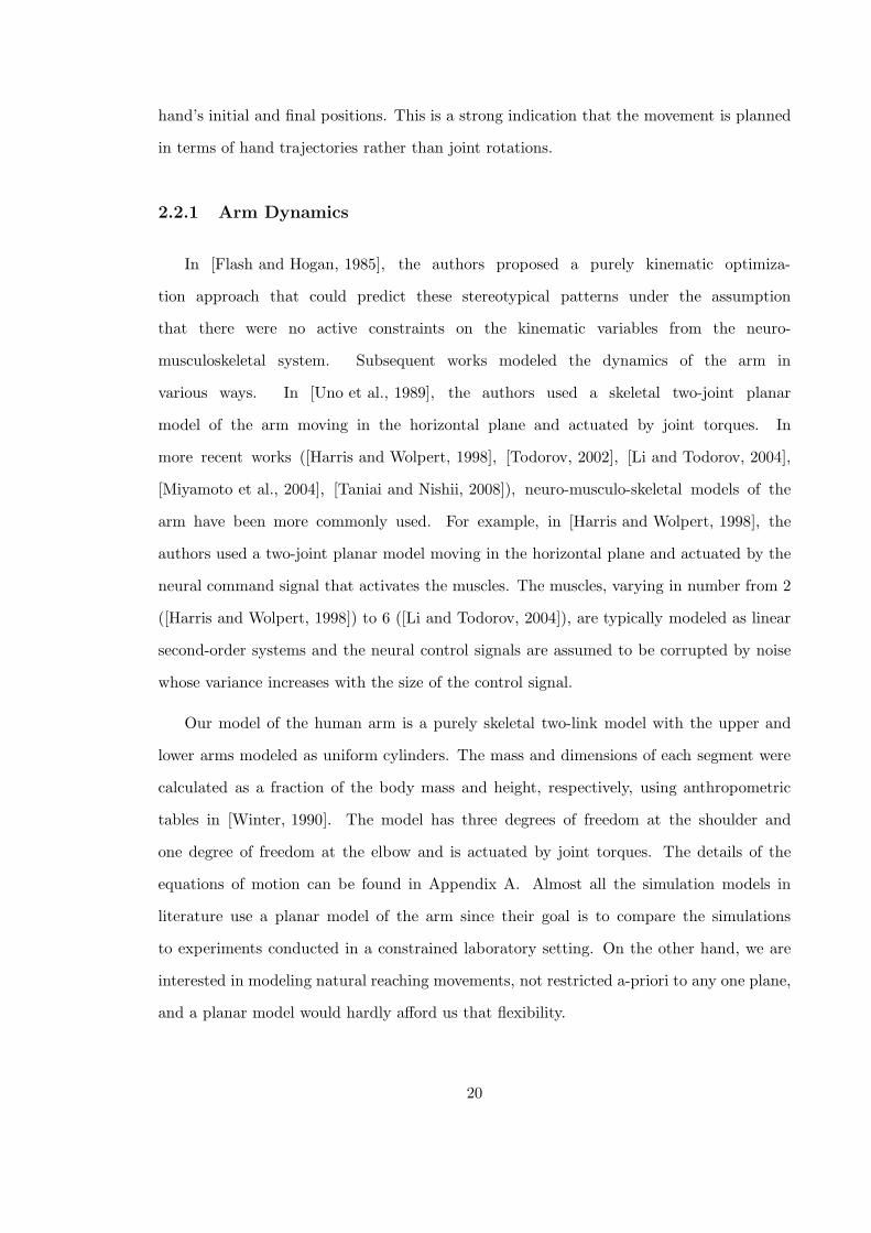
Our model of the human arm is a purely skeletal two-link model with the upper and
lower arms modeled as uniform cylinders. The mass and dimensions of each segment were
calculated as a fraction of the body mass and height, respectively, using anthropometric
tables in [Winter, 1990]. The model has three degrees of freedom at the shoulder and
one degree of freedom at the elbow and is actuated by joint torques. The details of the
equations of motion can be found in Appendix A. Almost all the simulation models in
literature use a planar model of the arm since their goal is to compare the simulations
to experiments conducted in a constrained laboratory setting. On the other hand, we are
interested in modeling natural reaching movements, not restricted a-priori to any one plane,
and a planar model would hardly afford us that flexibility.
20
Figure 2.1. Arm model. Our model of the human arm has three degrees of freedom at theshoulder (rotation about the three axes) and one degree of rotation, about the axis markedθe, at the elbow. The origin of the coordinate system is placed at the shoulder joint. Thepose shown is the reference pose, the pose at which all joint angles are zero. The x − zplane is referred to as the sagittal plane and the y− z plane is referred to as the transversalplane.
2.2.2 Cost Function for Reaching
Three different cost functions for reaching have been proposed in literature - the
minimum jerk model ([Hogan, 1984], [Flash and Hogan, 1985]), the minimum torque
change model ([Uno et al., 1989], [Nakano et al., 1999]) and the minimum variance model
([Harris and Wolpert, 1998]). The minimum jerk model, first proposed by [Hogan, 1984]
for single-joint forearm movements and [Flash and Hogan, 1985] for multi-joint arm move-
ments, states that the cost to be minimized is the derivative of the hand acceleration or
“jerk”. It is a purely kinematic optimization that does not model the arm dynamics at all.
For planar movements the cost function is
1
2
∫ T
0
(
(d3x
dt3)2 + (
d3y
dt3)2)
dt, (2.5)
21
where T is the fixed duration of the movement and (x, y) is the hand’s position at time t.
In the minimum torque change model proposed by [Uno et al., 1989] the cost function
for the planar two-joint arm is of the form
1
2
∫ T
0
(
(dτ1
dt)2 + (
dτ2
dt)2)
dt, (2.6)
where T is the fixed duration of the movement and τ1 and τ2 are the shoulder and elbow
torques, respectively, at time t. Both models force the hand to reach the target location by
imposing terminal constraints on the hand position and velocity. Thus, both the amplitude
(total distance travelled by the hand) and duration of the movemement is pre-determined.
The cost functions in Eq. (2.5) and Eq. (2.6) were both primarily engineered to produce
the smooth hand trajectories and bell-shaped hand velocity profiles observed in experiments
([Morasso, 1981], [Abend et al., 1982]). However, there is no principled explanation as to
why the central nervous system should have evolved to optimize these quantities.
In the minimum variance model proposed in [Harris and Wolpert, 1998], the shape
of the hand trajectory, parameterized as a cubic spline, is selected to minimize the variance
of the final hand position in the presence of signal-dependent noise in the neural control
signal. In this model smoothness of the hand trajectory arises naturally from the biological
fact of noisy neural signals - non-smooth movements require abrupt changes of muscle force
and large neural signals, which lead to increased control-dependent noise and poor accuracy
in the task.
Note that all three models have been successful in predicting the main characteris-
tics of point-to-point reaching movements, even though the minimum jerk model is purely
kinematic, the minimum torque change model uses a purely skeletal arm model actuated
by joint torques, and the minimum variance model uses a detailed neuro-musculo-skeletal
model of the arm. There have been critiques of the minimum jerk and minimum torque
change models. The minimum jerk model, since it ignores the nonlinear arm dynamics,
is inconsistent with the lack of symmetry observed in via-point tasks ([Uno et al., 1989],
[Nakano et al., 1999]) where the hand has to pass through multiple targets. On the other
hand, adaptation studies such as [Wolpert et al., 1995] have concluded that the cost function
for reaching is specified, at least in part, in kinematic coordinates, and that the adapta-
22
tions seen are incompatible with purely dynamic cost functions such as minimum torque
change. The strong kinematic component to trajectory planning is further supported by
the minimum variance model.
Energy minimization as a cost function has had limited success in explaining the invari-
ant features observed in reaching. In [Alexander, 1997] and [Nishii and Murakami, 2002] a
minimum energy cost criterion was tested and found to be successful in predicting hand
trajectories for reaching. However, the velocity profiles for the hand movements were con-
vex rather than bell-shaped. In both works the muscle dynamics and the noisy neural
control inputs to them were not modeled. In [Taniai and Nishii, 2008], the authors studied
the energy minimization criterion under the neuro-musculo-skeletal model used in the min-
imum variance approach described above and found both the hand trajectories and speed
profiles to be in agreement with experimental observations of reaching. However, energy
minimization as a criterion for arm trajectory planning is yet to be tested as extensively as
the minimum jerk, minimum torque change or minimum variance models.
At the same time, it is clear that energetics is an important factor in studying activation
patterns of individual muscles of the arm. A cost function combining accuracy and energy
was used to predict activation of individual arm muscles in [Todorov, 2002], and energy
minimization was used to predict activation patterns of wrist muscles in [Fagg et al., 2002].
In [Soechting et al., 1995] the authors reported that the final posture of the arm in three
dimensions could be predicted by the hypothesis that the final posture minimizes the amount
of work that must be done to transport the arm from the starting location.
More recent works such [Todorov, 2001] and [Miyamoto et al., 2004], as have taken the
view that the true performance criterion is likely a mix of cost terms combining accuracy and
energy. In [Miyamoto et al., 2004], the authors have proposed a criterion which is a weighted
sum of task achievement and energy consumption, where “task achievement” can be broadly
defined to include movements other than point-to-point reaching. The proposed model does
not require the pre-specification of the terminal boundary conditions for hand position and
velocity, though the duration of the movement is pre-specified. The performance criterion
was able to predict movement trajectories from a psychophysical experiment conducted
23
by the authors, but was less successful in predicting the velocity profiles. Interestingly,
the authors found that the trajectories were curved differently depending on the subject,
and by (manually) adjusting the weight in the optimization criterion combining the task
achievement and energy consumption terms, the shape of the trajectory could be reproduced
for all subjects.
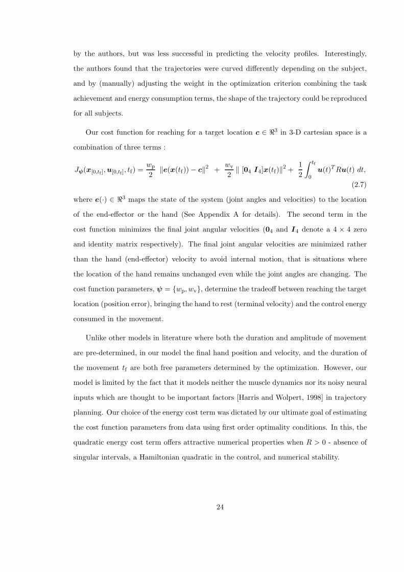
Our cost function for reaching for a target location c ∈ ℜ3 in 3-D cartesian space is a
combination of three terms :
Jψ(x[0,tf ],u[0,tf ], tf) =wp
2‖e(x(tf)) − c‖
2 +wv
2‖ [04 I4]x(tf)‖
2 +1
2
∫ tf
0u(t)T Ru(t) dt,
(2.7)
where e(·) ∈ ℜ3 maps the state of the system (joint angles and velocities) to the location
of the end-effector or the hand (See Appendix A for details). The second term in the
cost function minimizes the final joint angular velocities (04 and I4 denote a 4 × 4 zero
and identity matrix respectively). The final joint angular velocities are minimized rather
than the hand (end-effector) velocity to avoid internal motion, that is situations where
the location of the hand remains unchanged even while the joint angles are changing. The
cost function parameters, ψ = {wp, wv}, determine the tradeoff between reaching the target
location (position error), bringing the hand to rest (terminal velocity) and the control energy
consumed in the movement.
Unlike other models in literature where both the duration and amplitude of movement
are pre-determined, in our model the final hand position and velocity, and the duration of
the movement tf are both free parameters determined by the optimization. However, our
model is limited by the fact that it models neither the muscle dynamics nor its noisy neural
inputs which are thought to be important factors [Harris and Wolpert, 1998] in trajectory
planning. Our choice of the energy cost term was dictated by our ultimate goal of estimating
the cost function parameters from data using first order optimality conditions. In this, the
quadratic energy cost term offers attractive numerical properties when R > 0 - absence of
singular intervals, a Hamiltonian quadratic in the control, and numerical stability.
24
2.2.3 Simulation of Reaching
We solved the optimal control problem specified by the cost function in Eq. (2.7) and
the dynamical model described in Sec. 2.2.1 for different initial and target locations of the
hand, and for body masses in the range 65−85 kg and body heights in the range 1.6−1.8 m.
When the hand location is expressed in meters, the angular velocities in radians/second and
the joint torques in Newton-meters, the different terms in the cost function in Eq. (2.7) are
approximately in the same range. Therefore, for a given initial and target hand location,
body mass and height, we fixed the weight for the energy cost to be identity, i.e. R = I,
and varied the weights for position error (wp) and terminal velocity (wv). In this section
we discuss the trends and features observed in our simulations and compare them to those
observed in literature. All the trends and features discussed below were invariant to changes
in the initial and target locations of the hand and the body mass and height (See Figures
2.9 and 2.10).
0 0.5 1 1.5 2 2.5 3 3.5 40
0.1
0.2
0.3
0.4
0.5
0.6
0.7
0.8
0.9
1
log10
(wp)
Sca
led
Pos
ition
Err
or
log10
(wv)=0
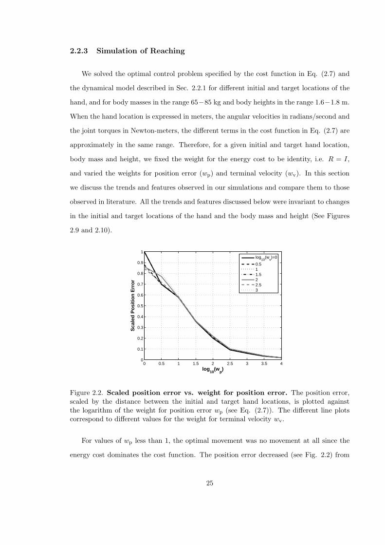
0.511.522.53
Figure 2.2. Scaled position error vs. weight for position error. The position error,scaled by the distance between the initial and target hand locations, is plotted againstthe logarithm of the weight for position error wp (see Eq. (2.7)). The different line plotscorrespond to different values for the weight for terminal velocity wv.
For values of wp less than 1, the optimal movement was no movement at all since the
energy cost dominates the cost function. The position error decreased (see Fig. 2.2) from
25
0 0.5 1 1.5 2 2.5 30
0.005
0.01
0.015
0.02
0.025
0.03
0.035
0.04
0.045
0.05
log10
(wv)
Fin
al H
and
Vel
ocity
in m
eter
s/se
c
log10
(wp) = 0
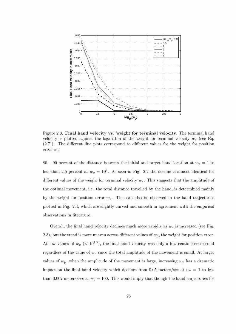
0.51234
Figure 2.3. Final hand velocity vs. weight for terminal velocity. The terminal handvelocity is plotted against the logarithm of the weight for terminal velocity wv (see Eq.(2.7)). The different line plots correspond to different values for the weight for positionerror wp.
80 − 90 percent of the distance between the initial and target hand location at wp = 1 to
less than 2.5 percent at wp = 104. As seen in Fig. 2.2 the decline is almost identical for
different values of the weight for terminal velocity wv. This suggests that the amplitude of
the optimal movement, i.e. the total distance travelled by the hand, is determined mainly
by the weight for position error wp. This can also be observed in the hand trajectories
plotted in Fig. 2.4, which are slightly curved and smooth in agreement with the empirical
observations in literature.
Overall, the final hand velocity declines much more rapidly as wv is increased (see Fig.
2.3), but the trend is more uneven across different values of wp, the weight for position error.
At low values of wp (< 101.5), the final hand velocity was only a few centimeters/second
regardless of the value of wv since the total amplitude of the movement is small. At larger
values of wp, when the amplitude of the movement is large, increasing wv has a dramatic
impact on the final hand velocity which declines from 0.05 meters/sec at wv = 1 to less
than 0.002 meters/sec at wv = 100. This would imply that though the hand trajectories for
26
0 0.2
0.40
0.20.4
0 0.08
−0.6
−0.55
−0.5
−0.45
−0.4
−0.35
x
log10
(wp) = 0.5
y
z
00.1
0.20.3
0.40.5
0 0.08
−0.6
−0.55
−0.5
−0.45
−0.4
−0.35
x
log10
(wp) = 1
y
z
00.1
0.20.3
0.40.5
0 0.08
−0.6
−0.55
−0.5
−0.45
−0.4
−0.35
x
log10
(wp) = 2
y
z
00.1
0.20.3
0.40.5
0 0.08
−0.6
−0.55
−0.5
−0.45
−0.4
−0.35
x
log10
(wp) = 3
y
z
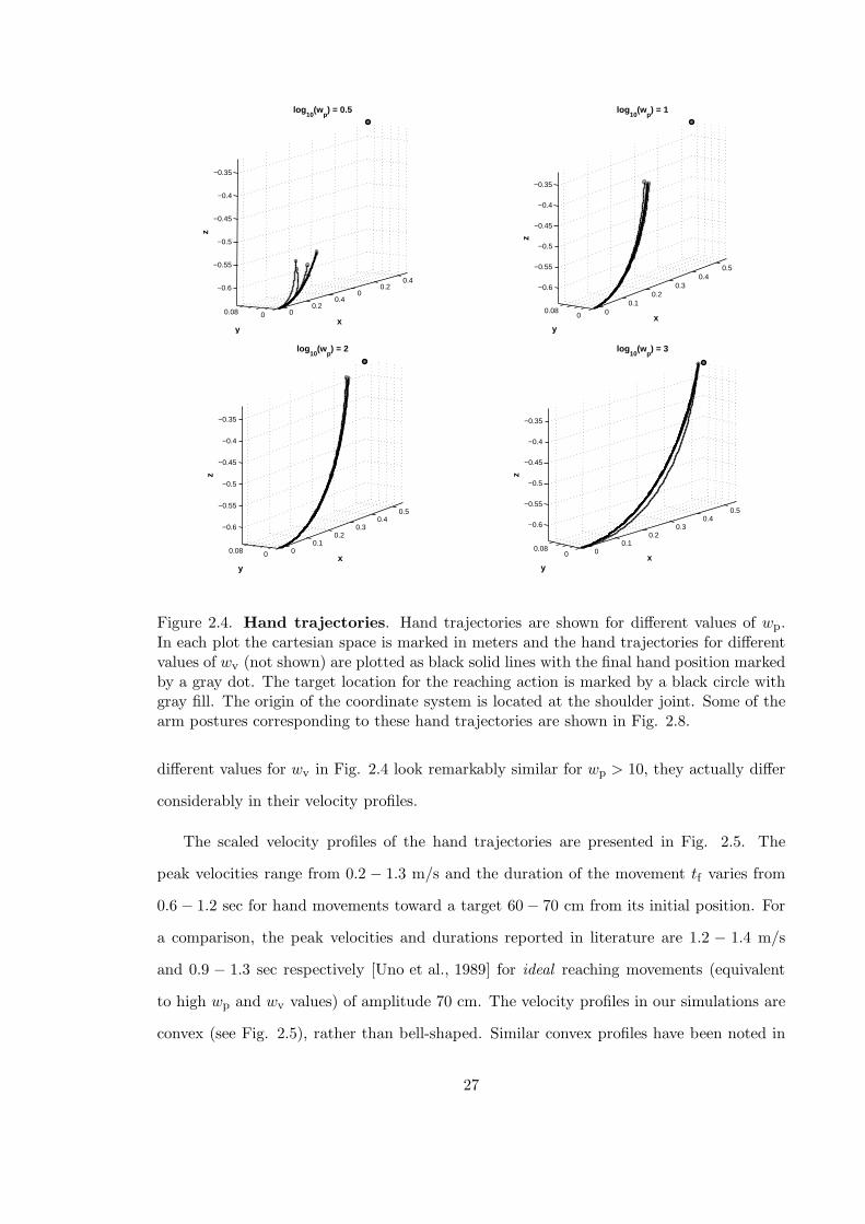
Figure 2.4. Hand trajectories. Hand trajectories are shown for different values of wp.In each plot the cartesian space is marked in meters and the hand trajectories for differentvalues of wv (not shown) are plotted as black solid lines with the final hand position markedby a gray dot. The target location for the reaching action is marked by a black circle withgray fill. The origin of the coordinate system is located at the shoulder joint. Some of thearm postures corresponding to these hand trajectories are shown in Fig. 2.8.
different values for wv in Fig. 2.4 look remarkably similar for wp > 10, they actually differ
considerably in their velocity profiles.
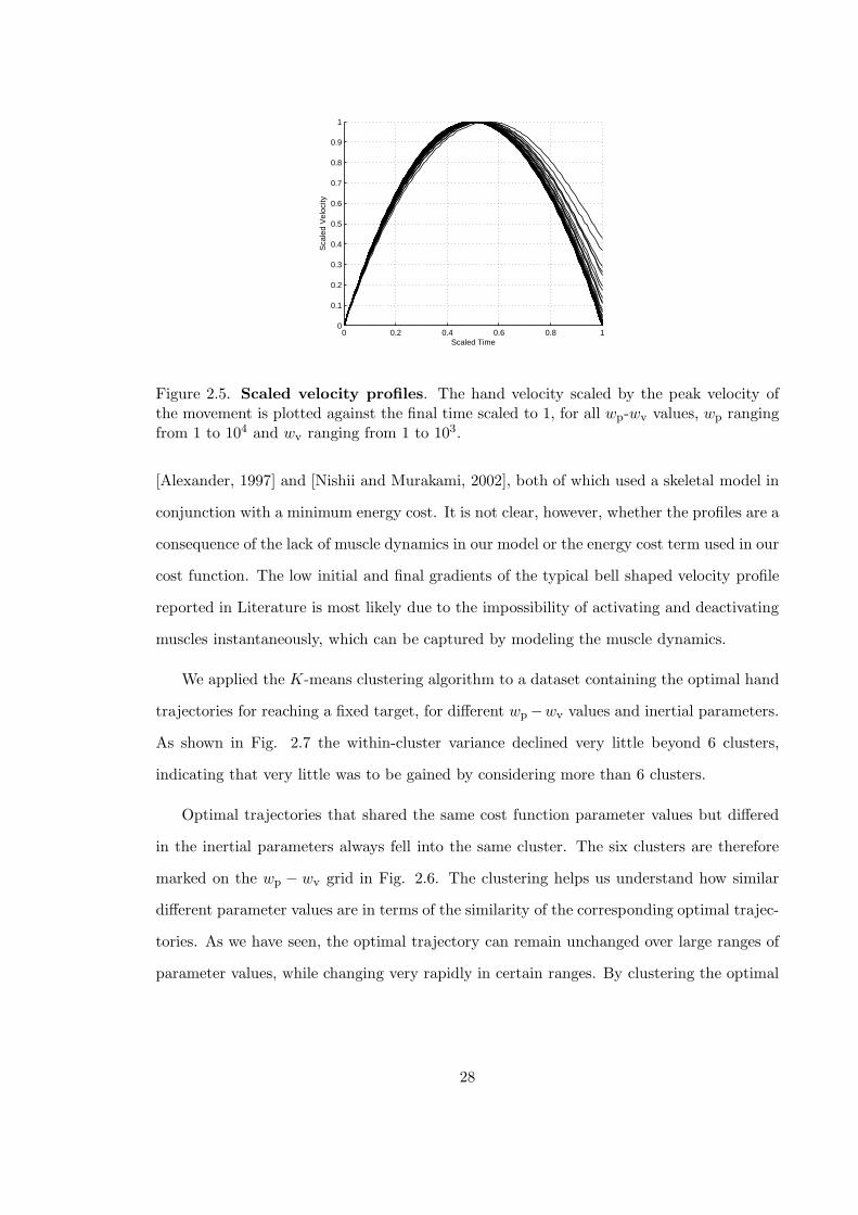
The scaled velocity profiles of the hand trajectories are presented in Fig. 2.5. The
peak velocities range from 0.2 − 1.3 m/s and the duration of the movement tf varies from
0.6 − 1.2 sec for hand movements toward a target 60 − 70 cm from its initial position. For
a comparison, the peak velocities and durations reported in literature are 1.2 − 1.4 m/s
and 0.9 − 1.3 sec respectively [Uno et al., 1989] for ideal reaching movements (equivalent
to high wp and wv values) of amplitude 70 cm. The velocity profiles in our simulations are
convex (see Fig. 2.5), rather than bell-shaped. Similar convex profiles have been noted in
27
0 0.2 0.4 0.6 0.8 10
0.1
0.2
0.3
0.4
0.5
0.6
0.7
0.8
0.9
1
Sca
led
Vel
ocity
Scaled Time
Figure 2.5. Scaled velocity profiles. The hand velocity scaled by the peak velocity ofthe movement is plotted against the final time scaled to 1, for all wp-wv values, wp rangingfrom 1 to 104 and wv ranging from 1 to 103.
[Alexander, 1997] and [Nishii and Murakami, 2002], both of which used a skeletal model in
conjunction with a minimum energy cost. It is not clear, however, whether the profiles are a
consequence of the lack of muscle dynamics in our model or the energy cost term used in our
cost function. The low initial and final gradients of the typical bell shaped velocity profile
reported in Literature is most likely due to the impossibility of activating and deactivating
muscles instantaneously, which can be captured by modeling the muscle dynamics.
We applied the K-means clustering algorithm to a dataset containing the optimal hand
trajectories for reaching a fixed target, for different wp −wv values and inertial parameters.
As shown in Fig. 2.7 the within-cluster variance declined very little beyond 6 clusters,
indicating that very little was to be gained by considering more than 6 clusters.
Optimal trajectories that shared the same cost function parameter values but differed
in the inertial parameters always fell into the same cluster. The six clusters are therefore
marked on the wp − wv grid in Fig. 2.6. The clustering helps us understand how similar
different parameter values are in terms of the similarity of the corresponding optimal trajec-
tories. As we have seen, the optimal trajectory can remain unchanged over large ranges of
parameter values, while changing very rapidly in certain ranges. By clustering the optimal
28
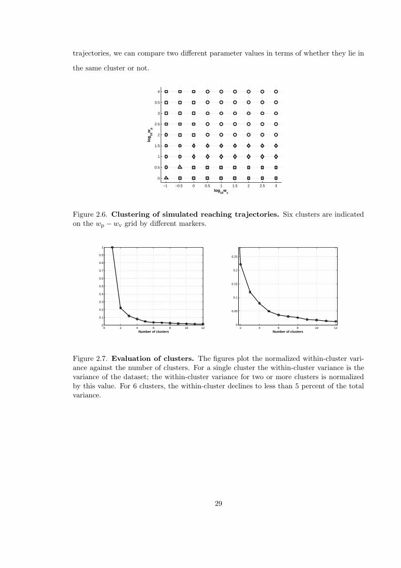
trajectories, we can compare two different parameter values in terms of whether they lie in
the same cluster or not.
−1 −0.5 0 0.5 1 1.5 2 2.5 3
0
0.5
1
1.5
2
2.5
3
3.5
4
log10
wv
log
10w
p
Figure 2.6. Clustering of simulated reaching trajectories. Six clusters are indicatedon the wp − wv grid by different markers.
0 2 4 6 8 10 120
0.1
0.2
0.3
0.4
0.5
0.6
0.7
0.8
0.9
1
Number of clusters2 4 6 8 10 12
0
0.05
0.1
0.15
0.2
0.25
Number of clusters
Figure 2.7. Evaluation of clusters. The figures plot the normalized within-cluster vari-ance against the number of clusters. For a single cluster the within-cluster variance is thevariance of the dataset; the within-cluster variance for two or more clusters is normalizedby this value. For 6 clusters, the within-cluster declines to less than 5 percent of the totalvariance.
29

0
0.2
0.4−0.6
−0.5
−0.4
−0.3
−0.2
−0.1
0
X
log10
(wp) = 1
Y
Z
shoulder
elbowhand
0
0.2
0.4−0.6
−0.5
−0.4
−0.3
−0.2
−0.1
0
X
log10
(wp) = 2
Y
Z
0
0.2
0.4−0.6
−0.5
−0.4
−0.3
−0.2
−0.1
0
X
log10
(wp) = 3
Y
Z
0
0.2
0.4−0.6
−0.5
−0.4
−0.3
−0.2
−0.1
0
X
log10
(wp) = 4
Y
Z
Figure 2.8. Arm postures in reaching. The figures show the arm postures for differentvalues of wp, wv = 1000. The shoulder, elbow and hand are visualized as red circles andthe target hand location is marked by a black circle with gray fill. The coordinate frame ismarked in meters, with the origin located at the shoulder. The direction of movement intime is marked by an arrow in the figure for wp = 10.
30
0 0.05 0.1 0.15 0.2 0.25 0.3 0.35 0.4 0.45 0.5−0.05
00.05
−0.65
−0.6
−0.55
−0.5
−0.45
−0.4
−0.35
x
z
y
1.8 m , 85 kg1.7 m , 85 kg1.7 m , 65 kg
0 0.2 0.4 0.6 0.8 10
0.2
0.4
0.6
0.8
1
1.2
1.4
Duration of Movement tf in seconds
Han
d V
eloc
ity in
met
ers/
sec
1.8 m , 85 kg1.7 m , 85 kg1.7 m , 65 kg
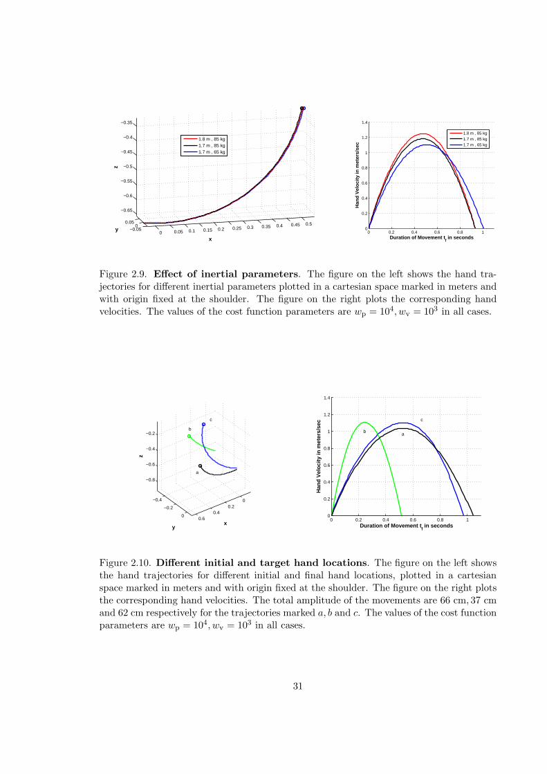
Figure 2.9. Effect of inertial parameters. The figure on the left shows the hand tra-jectories for different inertial parameters plotted in a cartesian space marked in meters andwith origin fixed at the shoulder. The figure on the right plots the corresponding handvelocities. The values of the cost function parameters are wp = 104, wv = 103 in all cases.
00.2
0.40.6
−0.4
−0.2
0
−0.8
−0.6
−0.4
−0.2
xy
z
a
b
c
0 0.2 0.4 0.6 0.8 10
0.2
0.4
0.6
0.8
1
1.2
1.4
Duration of Movement tf in seconds
Han
d V
eloc
ity in
met
ers/
sec
ab
c
Figure 2.10. Different initial and target hand locations. The figure on the left showsthe hand trajectories for different initial and final hand locations, plotted in a cartesianspace marked in meters and with origin fixed at the shoulder. The figure on the right plotsthe corresponding hand velocities. The total amplitude of the movements are 66 cm, 37 cmand 62 cm respectively for the trajectories marked a, b and c. The values of the cost functionparameters are wp = 104, wv = 103 in all cases.
31
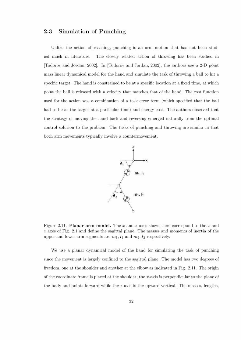
2.3 Simulation of Punching
Unlike the action of reaching, punching is an arm motion that has not been stud-
ied much in literature. The closely related action of throwing has been studied in
[Todorov and Jordan, 2002]. In [Todorov and Jordan, 2002], the authors use a 2-D point
mass linear dynamical model for the hand and simulate the task of throwing a ball to hit a
specific target. The hand is constrained to be at a specific location at a fixed time, at which
point the ball is released with a velocity that matches that of the hand. The cost function
used for the action was a combination of a task error term (which specified that the ball
had to be at the target at a particular time) and energy cost. The authors observed that
the strategy of moving the hand back and reversing emerged naturally from the optimal
control solution to the problem. The tasks of punching and throwing are similar in that
both arm movements typically involve a countermovement.
Figure 2.11. Planar arm model. The x and z axes shown here correspond to the x andz axes of Fig. 2.1 and define the sagittal plane. The masses and moments of inertia of theupper and lower arm segments are m1, I1 and m2, I2 respectively.
We use a planar dynamical model of the hand for simulating the task of punching
since the movement is largely confined to the sagittal plane. The model has two degrees of
freedom, one at the shoulder and another at the elbow as indicated in Fig. 2.11. The origin
of the coordinate frame is placed at the shoulder; the x-axis is perpendicular to the plane of
the body and points forward while the z-axis is the upward vertical. The masses, lengths,
32

centers of mass and moments of inertia of the two links were obtained as a fraction of the
total body height and mass using the anthropometric tables in [Winter, 1990]. The details
of the equations of motion can be found in Appendix B. Our cost function for punching a
target at location c ∈ ℜ2 in 2-D cartesian space is a combination of three terms:
Jψ(x[0,tf ],u[0,tf ], tf) =wp
2‖e(x(tf)) − c‖
2 −wv
2sgn(ex(x(tf))) ‖ex(x(tf))‖
2
+1
2
∫ tf
0u(t)T Ru(t) dt, (2.8)
where e(·) ∈ ℜ2 maps the state of the system (joint angles and velocities) to the location
of the end-effector i.e. the hand in the sagittal plane (See Appendix B for details). The
function ex(·) maps the state of the system to the final velocity of the hand along the x-
axis. The cost function parameters ψ = {wp, wv} determine the tradeoff between reaching
the target location (position error), maximizing the final hand velocity along the positive
x-axis and the control energy consumed in the movement. The final hand position and
velocity, and the duration of the movement tf are both free parameters determined by the
optimization. The task of throwing could be similarly modeled by maximizing the final
hand velocity in a particular direction.
We solved the optimal control problem specified by the cost function in Eq. (2.8) and
the dynamical model described above, for different initial and target locations of the hand,
and for body masses in the range 65− 85 kg and body heights in the range 1.6− 1.8 m. For
a given initial and target hand location, body mass and height, we fixed the weight for the
energy cost to be identity, i.e. R = I, and varied the weights for position error (wp) and
terminal velocity (wv) in the range 1 to 106. The results discussed below are for a body
height of 1.65 m and mass of 60 kg, but as shown in Fig. 2.15 the variation of inertial
parameters has negligible effect on the optimal trajectory.
33
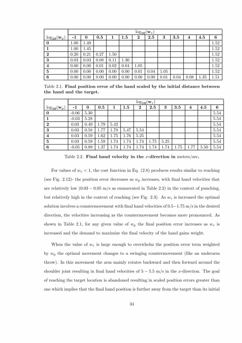
log10(wv)log10(wp) -1 0 0.5 1 1.5 2 2.5 3 3.5 4 4.5 6
0 1.00 1.49 1.52
1 1.00 1.45 1.52
2 0.20 0.21 0.27 1.50 1.52
3 0.03 0.03 0.08 0.11 1.36 1.52
4 0.00 0.00 0.01 0.02 0.04 1.05 1.52
5 0.00 0.00 0.00 0.00 0.00 0.01 0.04 1.05 1.52
6 0.00 0.00 0.00 0.00 0.00 0.00 0.00 0.01 0.04 0.08 1.35 1.51
Table 2.1. Final position error of the hand scaled by the initial distance betweenthe hand and the target.
log10(wv)log10(wp) -1 0 0.5 1 1.5 2 2.5 3 3.5 4 4.5 6
0 -0.06 5.30 5.54
1 -0.03 5.28 5.54
2 0.03 0.49 1.79 5.42 5.54
3 0.03 0.58 1.77 1.78 5.47 5.54 5.54
4 0.03 0.59 1.62 1.75 1.76 5.25 5.54
5 0.03 0.59 1.59 1.74 1.74 1.74 1.75 5.25 5.54
6 -0.05 0.89 1.37 1.74 1.74 1.74 1.74 1.74 1.75 1.77 5.50 5.54
Table 2.2. Final hand velocity in the x-direction in meters/sec.
For values of wv < 1, the cost function in Eq. (2.8) produces results similar to reaching
(see Fig. 2.12)- the position error decreases as wp increases, with final hand velocities that
are relatively low (0.03 − 0.05 m/s as enumerated in Table 2.2) in the context of punching,
but relatively high in the context of reaching (see Fig. 2.3). As wv is increased the optimal
solution involves a countermovement with final hand velocities of 0.5−1.75 m/s in the desired
direction, the velocities increasing as the countermovement becomes more pronounced. As
shown in Table 2.1, for any given value of wp the final position error increases as wv is
increased and the demand to maximize the final velocity of the hand gains weight.
When the value of wv is large enough to overwhelm the position error term weighted
by wp the optimal movement changes to a swinging countermovement (like an underarm
throw). In this movement the arm mainly rotates backward and then forward around the
shoulder joint resulting in final hand velocities of 5 − 5.5 m/s in the x-direction. The goal
of reaching the target location is abandoned resulting in scaled position errors greater than
one which implies that the final hand position is further away from the target than its initial
34
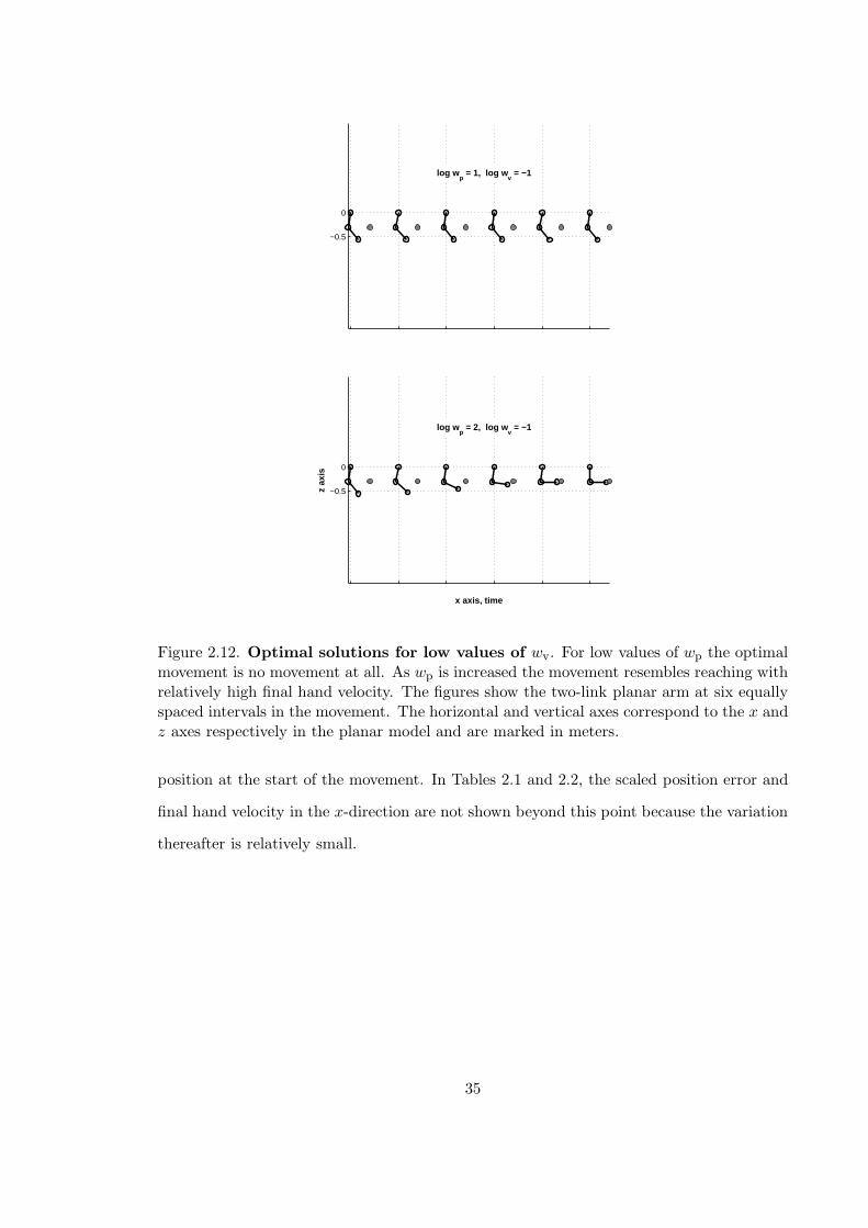
−0.5
0
log wp = 1, log w
v = −1
−0.5
0
log wp = 2, log w
v = −1
x axis, time
z ax
is
Figure 2.12. Optimal solutions for low values of wv. For low values of wp the optimalmovement is no movement at all. As wp is increased the movement resembles reaching withrelatively high final hand velocity. The figures show the two-link planar arm at six equallyspaced intervals in the movement. The horizontal and vertical axes correspond to the x andz axes respectively in the planar model and are marked in meters.
position at the start of the movement. In Tables 2.1 and 2.2, the scaled position error and
final hand velocity in the x-direction are not shown beyond this point because the variation
thereafter is relatively small.
35
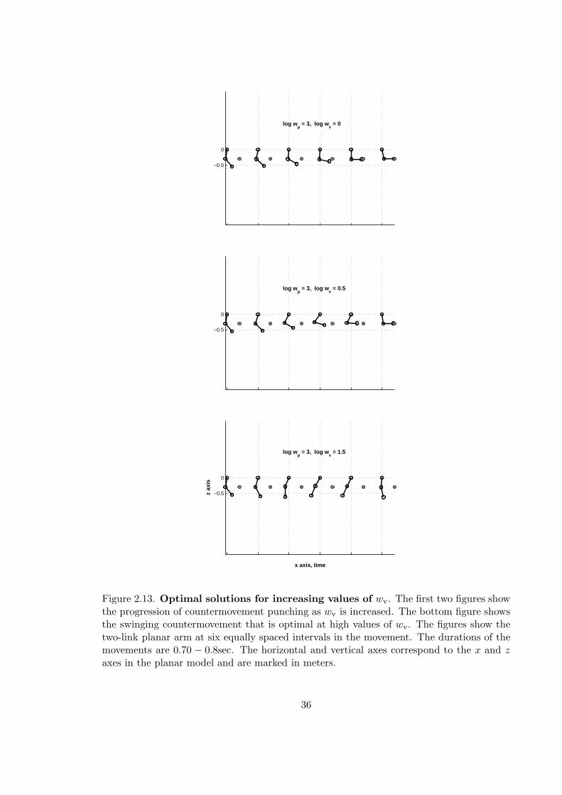
−0.5
0
log wp = 3, log w
v = 0
−0.5
0
log wp = 3, log w
v = 0.5
−0.5
0
log wp = 3, log w
v = 1.5
x axis, time
z ax
is
Figure 2.13. Optimal solutions for increasing values of wv. The first two figures showthe progression of countermovement punching as wv is increased. The bottom figure showsthe swinging countermovement that is optimal at high values of wv. The figures show thetwo-link planar arm at six equally spaced intervals in the movement. The durations of themovements are 0.70 − 0.8sec. The horizontal and vertical axes correspond to the x and zaxes in the planar model and are marked in meters.
36
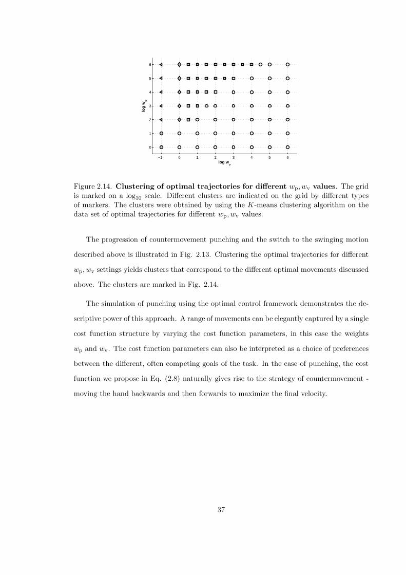
−1 0 1 2 3 4 5 6
0
1
2
3
4
5
6
log wv
log
wp
Figure 2.14. Clustering of optimal trajectories for different wp, wv values. The gridis marked on a log10 scale. Different clusters are indicated on the grid by different typesof markers. The clusters were obtained by using the K-means clustering algorithm on thedata set of optimal trajectories for different wp, wv values.
The progression of countermovement punching and the switch to the swinging motion
described above is illustrated in Fig. 2.13. Clustering the optimal trajectories for different
wp, wv settings yields clusters that correspond to the different optimal movements discussed
above. The clusters are marked in Fig. 2.14.
The simulation of punching using the optimal control framework demonstrates the de-
scriptive power of this approach. A range of movements can be elegantly captured by a single
cost function structure by varying the cost function parameters, in this case the weights
wp and wv. The cost function parameters can also be interpreted as a choice of preferences
between the different, often competing goals of the task. In the case of punching, the cost
function we propose in Eq. (2.8) naturally gives rise to the strategy of countermovement -
moving the hand backwards and then forwards to maximize the final velocity.
37
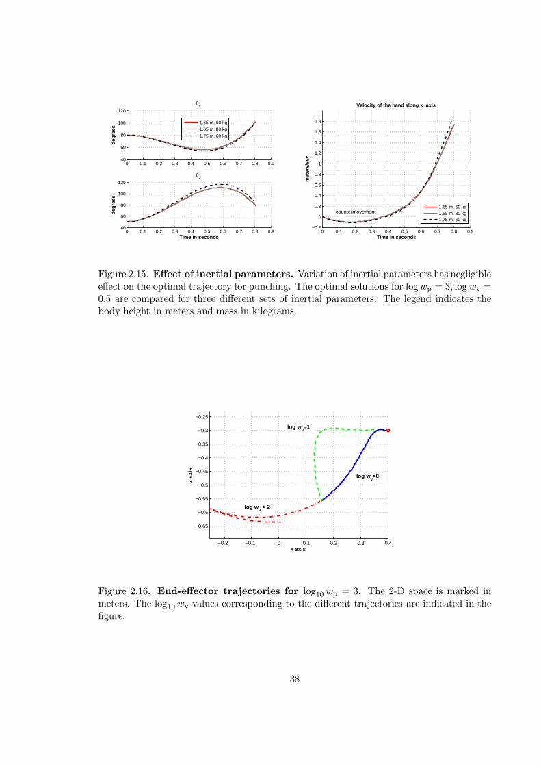
0 0.1 0.2 0.3 0.4 0.5 0.6 0.7 0.8 0.940
60
80
100
120de
gree
s
θ1
0 0.1 0.2 0.3 0.4 0.5 0.6 0.7 0.8 0.940
60
80
100
120
Time in seconds
θ2
degr
ees
1.65 m, 60 kg
1.65 m, 80 kg
1.75 m, 60 kg
0 0.1 0.2 0.3 0.4 0.5 0.6 0.7 0.8 0.9−0.2
0
0.2
0.4
0.6
0.8
1
1.2
1.4
1.6
1.8
Time in seconds
met
ers/
sec
Velocity of the hand along x−axis
countermovement1.65 m, 60 kg1.65 m, 80 kg1.75 m, 60 kg
Figure 2.15. Effect of inertial parameters. Variation of inertial parameters has negligibleeffect on the optimal trajectory for punching. The optimal solutions for log wp = 3, log wv =0.5 are compared for three different sets of inertial parameters. The legend indicates thebody height in meters and mass in kilograms.
−0.2 −0.1 0 0.1 0.2 0.3 0.4
−0.65
−0.6
−0.55
−0.5
−0.45
−0.4
−0.35
−0.3
−0.25
x axis
z ax
is
log wv > 2
log wv=0
log wv=1
Figure 2.16. End-effector trajectories for log10 wp = 3. The 2-D space is marked inmeters. The log10 wv values corresponding to the different trajectories are indicated in thefigure.
38

2.4 Conclusion
An advantage of using the optimal control framework to model human actions is that the
cost function can be constructed from our intuitive understanding of the task definition.
However the interaction between the cost function and the nonlinear body dynamics is
complex. By using numerical methods to solve the optimal control problem for different
parameter settings and inertial parameters we can get a better sense of the range of motions
that can be produced by the cost function we have proposed.
While numerical methods have been used to simulate optimal trajectories which are
then compared to experimental data, the cost function parameter values in these studies
are fixed by trial-and-error to calibrate the model to data. The objective is to study an
ideal average prototypical motion. On the other hand, our goal is to explore the full range
of motions that can be produced by a single cost function.
Our simulations of two arm motions - reaching and punching - indicate that the optimal
trajectory can vary very little over some parameter ranges while changing rapidly in others.
This implies that the euclidean distance between two parameter values is a poor indicator
of how “close” they are, since the most natural measure of the “closeness” of two parameter
values would be the similarity of the optimal trajectories they produce. A better way to
make a judgement on whether two parameter values are close would be to check whether
they lie in the same cluster or not.
Our simulations of arm motions also show that variation of inertial parameters has
negligible effect on the optimal trajectory, especially when compared to the impact of pa-
rameter variation. This indicates that for some actions it is possible to have a common
interpretation of cost function parameters for different people; that is we can compare the
cost function parameter values of two people directly without referencing their body heights
and masses. However, this feature might not hold for all human actions.
39
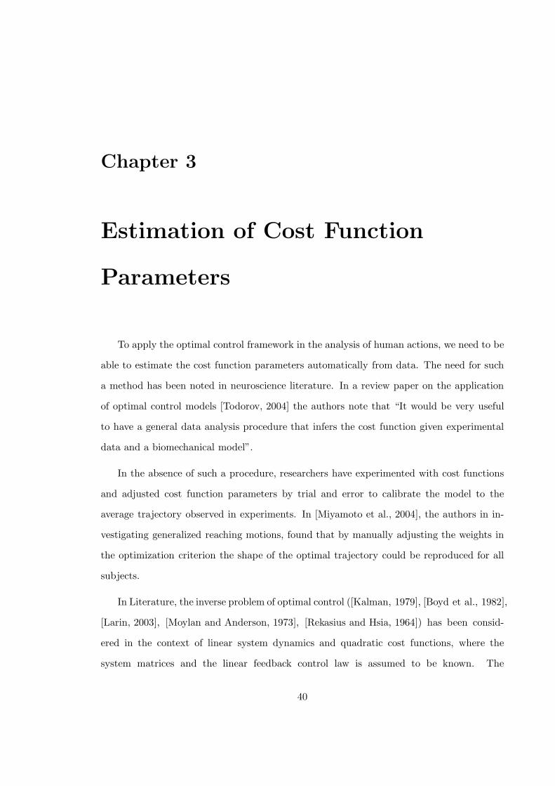
Chapter 3
Estimation of Cost Function
Parameters
To apply the optimal control framework in the analysis of human actions, we need to be
able to estimate the cost function parameters automatically from data. The need for such
a method has been noted in neuroscience literature. In a review paper on the application
of optimal control models [Todorov, 2004] the authors note that “It would be very useful
to have a general data analysis procedure that infers the cost function given experimental
data and a biomechanical model”.
In the absence of such a procedure, researchers have experimented with cost functions
and adjusted cost function parameters by trial and error to calibrate the model to the
average trajectory observed in experiments. In [Miyamoto et al., 2004], the authors in in-
vestigating generalized reaching motions, found that by manually adjusting the weights in
the optimization criterion the shape of the optimal trajectory could be reproduced for all
subjects.
In Literature, the inverse problem of optimal control ([Kalman, 1979], [Boyd et al., 1982],
[Larin, 2003], [Moylan and Anderson, 1973], [Rekasius and Hsia, 1964]) has been consid-
ered in the context of linear system dynamics and quadratic cost functions, where the
system matrices and the linear feedback control law is assumed to be known. The
40
problem then is to determine the weighting matrices in the quadratic cost function,
such that the given control law is optimal with respect to it. The problem was first
proposed in [Kalman, 1979], and several methods have been proposed ([Larin, 2003],
[Moylan and Anderson, 1973],[Rekasius and Hsia, 1964]), including the use of Linear Ma-
trix Inequalities (LMI) [Boyd et al., 1982], to solve the problem. Given the nonlinearity
of our biomechanical models and cost functions (which are quadratic only in the control),
these solutions are not applicable in the problems we consider.
In the related field of reinforcement learning the problem of learning the reward function
from observed optimal behavior has been addressed in [Ng and Russell, 2000], where it
is solved as linear program, and in [Ramachandran and Amir, 2007] where a probability
distribution over the space of reward functions is determined. In [Ng and Russell, 2000] the
authors identify degeneracy - the existence of a large set of reward functions for which the
observed behavior is optimal - as the key issue, and address it by using heuristics to pick a
reward function.
In its most general form the problem definition would be as follows: given an optimal
trajectory and a known system dynamics, can we determine the cost function with respect
to which the trajectory is optimal? We address this problem in a more limited setting,
where the structure of the cost function is known, while certain parameters are considered
unknown. In this chapter we propose a method to estimate the unknown cost function
parameters from data and demonstrate the use of the method on two tasks: reaching and
punching.
3.1 Methods
Consider the time-discretized form of the free-final time optimal control problem pre-
sented in Eq. (2.3) and Eq. (2.4):
minx1,...,xM ,u1,...,uM ,tf
Jψ(x1, . . . ,xM ,u1, . . . ,uM , tf)
s.t. gk = 0 k = 1, . . . ,M. (3.1)
41

where
Jψ = hψ(xM )︸ ︷︷ ︸
F inal cost
+tf
2(M − 1)
(
1
2uT
1 Ru1 +
M−1∑
k=2
uTk Ruk +
1
2uT
MRuM
)
︸ ︷︷ ︸
Energy Cost
(3.2)
and
g1 = x1 − x0
gk = xk − xk−1 −tf
2(M − 1)(f(xk,uk) + f(xk−1,uk−1)) , k = 2, . . . ,M. (3.3)
The subscript ψ in the cost function J and the final cost h(·) indicate that these functions
are parameterized by the cost function parameters ψ which we wish to estimate. The energy
cost R is held at a fixed value while other parameters (weights) are estimated relative to it.
In Eq. (3.3), x0 is the known initial state of the biomechanical system, whose continuous-
time dynamics are described the nonlinear differential equations x(t) = f(x(t),u(t)).
Any solution to the optimization problem in Eq. (3.1) will satisfy the following first
order necessary conditions:
∂Jψ∂xk
+ λT1
∂g1
∂xk
+ . . . + λTM
∂gM
∂xk
= 0 (3.4)
∂Jψ∂uk
+ λT1
∂g1
∂uk
+ . . . + λTM
∂gM
∂uk
= 0 (3.5)
∂Jψ∂tf
+ λT1
∂g1
∂tf+ . . . + λT
M
∂gM
∂tf= 0 (3.6)
for k = 1, . . . ,M , that is the gradient of the objective has to be orthogonal to the constraint
surface. In addition to the above conditions the optimal trajectory also has to lie on the
constraint surface and satisfy the constraints in Eq. (3.3). These are the time-discretized
version of the necessary conditions (two-point boundary value problem) in Eq. (1.12). The
Lagrange multipliers λ1, . . . ,λM are the discrete-time equivalent of the costate trajectory.
The Equations (3.3), (3.4), (3.5) and (3.6) are the discrete-time equivalents of the state,
costate, control and terminal (boundary) conditions respectively. Since our system dynamics
are linear in the control and the cost function is quadratic in the control with Huu =
R > 0 by construction, the Hessian of the Hamiltonian with respect to the control will be
positive-definite everywhere. Therefore, the strengthened Legendre-Clebsch [Stengel, 1994]
42
(or convexity) condition (Huu > 0), the sufficient condition for optimality, will be satisfied
for any trajectory which satisfies the necessary conditions.
Let x1:M denote the set of variables {x1,x2, . . . ,xM}. We shall use the notation
(x1:M ,u1:M ,λ1:M , tf) to denote a set of state, control, Lagrange multiplier and final time
values which may or may not satisfy the necessary conditions described above; optimal
values are denoted by (x∗
1:M ,u∗
1:M ,λ∗
1:M , t∗f ) and will satisfy the conditions. In estimating
cost function parameters from data, we assume that the trajectory we observe is optimal
for some set of parameters. Thus the optimal state trajectory x∗
1:M and the final time t∗f is
known to us. We also assume that the biomechanical model and its dynamics are known
to us. As we saw in the previous chapter, given the body height and mass of the subject
performing the action, we can obtain all the required inertial values for the biomechanical
model. We do not require detailed limb measurements of our subjects. Since the body
dynamics are known, the optimal control (torques) trajectory u∗
1:M can also be obtained
directly from the data. Further details on these data processing steps are given in Sec. 3.2.
For the fixed (x∗
1:M ,u∗
1:M , t∗f ) values obtained from data, if we can find a set of cost func-
tion parameters ψ and Lagrange multipliers λ∗
1:M , such that Eq. (3.4)-(3.6) are satisfied, we
can be rest assured that the observed trajectory is at optimal for the obtained cost function
parameters. Since the number of cost function parameters is usually small, this problem is
overdetermined. We therefore treat Eq. (3.4)-(3.6) as a least squares optimization problem
and solve for cost function parameters and Lagrange multiplier values that satisfy these
equations approximately.
For the biomechanical system models we consider the dynamics are of the form
f(xk,uk) = A(xk) + B(xk)uk. (3.7)
Therefore Eq. (3.4)-(3.6) are of the form stated below where ∆ = tf/(M − 1), I denotes an
identity matrix of the appropriate dimensions, and fx is the partial derivative of the system
43
dynamics with respect to the state.
λ1 − (I +∆
2fx(xk,uk))
Tλ2 = 0
(I −∆
2fx(xk,uk))
Tλk − (I +∆
2fx(xk,uk))
Tλk+1 = 0 k = 2, . . . ,M − 1
∂hψ∂x
(xM ) + (I −∆
2fx(xM ,uM ))TλM = 0 (3.8)
B(x1)Tλ2 − Ru1 = 0
B(xk)Tλk + B(xk)
Tλk+1 = 2Ruk k = 2, . . . ,M − 1
B(xM )TλM − RuM = 0 (3.9)
M∑
k=2
(f(xk,uk) + f(xk−1,uk−1))Tλk =
1
2uT
1 Ru1 +
M−1∑
k=2
uTk Ruk +
1
2uT
MRuM
(3.10)
All partial derivatives of the constraint equations can be computed (through finite dif-
ferences) along the optimal state and control trajectory we observe and are constants in the
least squares optimization to find the cost function parameters and Lagrange multipliers.
In our formulation we do not consider inequality constraints on joint angles, velocities
(state) or torques (control). Firstly, precise lower and upper bounds for these are difficult to
determine. Secondly, for everyday movements we can reasonably assume that the subjects
do not operate near the limits and that the constraints are inactive.
As we observed in the previous chapter, in the simulation of reaching and punching
actions, entire ranges of parameter values could give rise to very similar optimal trajectories.
Therefore in comparing parameter estimates to actual values, or to each other, we use the
clustering of the simulated optimal trajectories - parameter values that lie in the same
cluster are evaluated as being close.
44
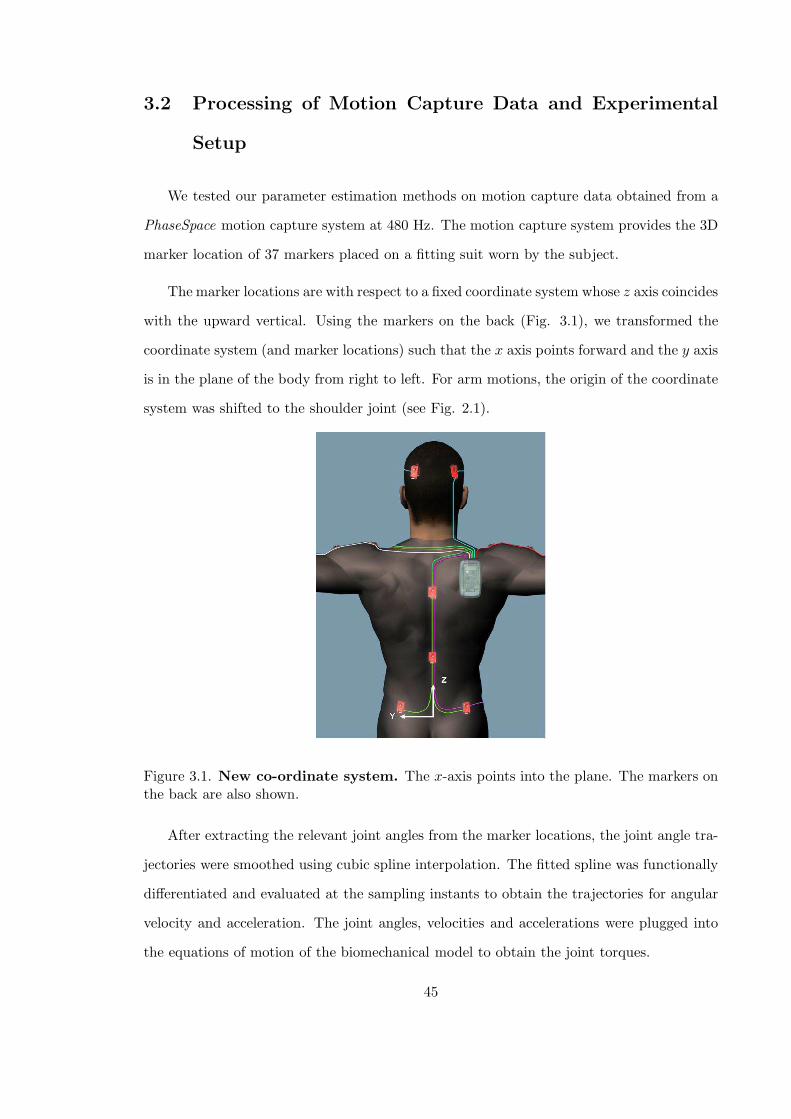
3.2 Processing of Motion Capture Data and Experimental
Setup
We tested our parameter estimation methods on motion capture data obtained from a
PhaseSpace motion capture system at 480 Hz. The motion capture system provides the 3D
marker location of 37 markers placed on a fitting suit worn by the subject.
The marker locations are with respect to a fixed coordinate system whose z axis coincides
with the upward vertical. Using the markers on the back (Fig. 3.1), we transformed the
coordinate system (and marker locations) such that the x axis points forward and the y axis
is in the plane of the body from right to left. For arm motions, the origin of the coordinate
system was shifted to the shoulder joint (see Fig. 2.1).
Figure 3.1. New co-ordinate system. The x-axis points into the plane. The markers onthe back are also shown.
After extracting the relevant joint angles from the marker locations, the joint angle tra-
jectories were smoothed using cubic spline interpolation. The fitted spline was functionally
differentiated and evaluated at the sampling instants to obtain the trajectories for angular
velocity and acceleration. The joint angles, velocities and accelerations were plugged into
the equations of motion of the biomechanical model to obtain the joint torques.
45
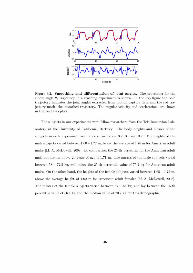
10 15 20 250
10
20
deg
10 15 20 25−50
0
50
deg/
sec
10 15 20 25
−200
0
200
seconds
deg/
sec
2
Figure 3.2. Smoothing and differentiation of joint angles. The processing for theelbow angle θe trajectory in a reaching experiment is shown. In the top figure the bluetrajectory indicates the joint angles extracted from motion capture data and the red tra-jectory marks the smoothed trajectory. The angular velocity and accelerations are shownin the next two plots.
The subjects in our experiments were fellow-researchers from the Tele-Immersion Lab-
oratory at the University of California, Berkeley. The body heights and masses of the
subjects in each experiment are indicated in Tables 3.2, 3.3 and 3.7. The heights of the
male subjects varied between 1.60−1.72 m, below the average of 1.76 m for American adult
males [M. A. McDowell, 2008]; for comparison the 25-th percentile for the American adult
male population above 20 years of age is 1.71 m. The masses of the male subjects varied
between 58 − 72.5 kg, well below the 25-th percentile value of 75.2 kg for American adult
males. On the other hand, the heights of the female subjects varied between 1.65− 1.75 m,
above the average height of 1.62 m for American adult females [M. A. McDowell, 2008].
The masses of the female subjects varied between 57 − 68 kg, and lay between the 15-th
percentile value of 56.1 kg and the median value of 70.7 kg for this demographic.
46
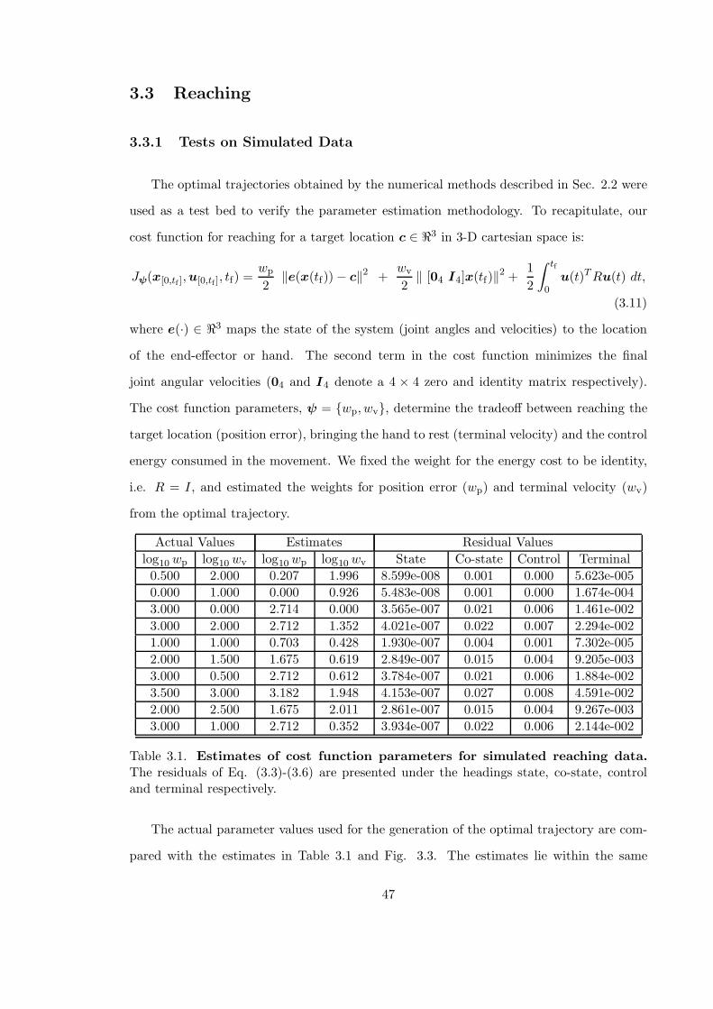
3.3 Reaching
3.3.1 Tests on Simulated Data
The optimal trajectories obtained by the numerical methods described in Sec. 2.2 were
used as a test bed to verify the parameter estimation methodology. To recapitulate, our
cost function for reaching for a target location c ∈ ℜ3 in 3-D cartesian space is:
Jψ(x[0,tf ],u[0,tf ], tf) =wp
2‖e(x(tf)) − c‖
2 +wv
2‖ [04 I4]x(tf)‖
2 +1
2
∫ tf
0u(t)T Ru(t) dt,
(3.11)
where e(·) ∈ ℜ3 maps the state of the system (joint angles and velocities) to the location
of the end-effector or hand. The second term in the cost function minimizes the final
joint angular velocities (04 and I4 denote a 4 × 4 zero and identity matrix respectively).
The cost function parameters, ψ = {wp, wv}, determine the tradeoff between reaching the
target location (position error), bringing the hand to rest (terminal velocity) and the control
energy consumed in the movement. We fixed the weight for the energy cost to be identity,
i.e. R = I, and estimated the weights for position error (wp) and terminal velocity (wv)
from the optimal trajectory.
Actual Values Estimates Residual Values
log10 wp log10 wv log10 wp log10 wv State Co-state Control Terminal
0.500 2.000 0.207 1.996 8.599e-008 0.001 0.000 5.623e-005
0.000 1.000 0.000 0.926 5.483e-008 0.001 0.000 1.674e-004
3.000 0.000 2.714 0.000 3.565e-007 0.021 0.006 1.461e-002
3.000 2.000 2.712 1.352 4.021e-007 0.022 0.007 2.294e-002
1.000 1.000 0.703 0.428 1.930e-007 0.004 0.001 7.302e-005
2.000 1.500 1.675 0.619 2.849e-007 0.015 0.004 9.205e-003
3.000 0.500 2.712 0.612 3.784e-007 0.021 0.006 1.884e-002
3.500 3.000 3.182 1.948 4.153e-007 0.027 0.008 4.591e-002
2.000 2.500 1.675 2.011 2.861e-007 0.015 0.004 9.267e-003
3.000 1.000 2.712 0.352 3.934e-007 0.022 0.006 2.144e-002
Table 3.1. Estimates of cost function parameters for simulated reaching data.The residuals of Eq. (3.3)-(3.6) are presented under the headings state, co-state, controland terminal respectively.
The actual parameter values used for the generation of the optimal trajectory are com-
pared with the estimates in Table 3.1 and Fig. 3.3. The estimates lie within the same
47

cluster as the actual parameter value, even if they do, in some cases, tend to move to the
edge of the cluster (See the bottom two figures in Fig. 3.3).
48

−1 −0.5 0 0.5 1 1.5 2 2.5 3
0
0.5
1
1.5
2
2.5
3
3.5
4
log10
wv
log
10w
p
−1 −0.5 0 0.5 1 1.5 2 2.5 3
0
0.5
1
1.5
2
2.5
3
3.5
4
log10
wv
log
10w
p
−1 −0.5 0 0.5 1 1.5 2 2.5 3
0
0.5
1
1.5
2
2.5
3
3.5
4
log10
wv
log
10w
p
−1 −0.5 0 0.5 1 1.5 2 2.5 3
0
0.5
1
1.5
2
2.5
3
3.5
4
log10
wv
log
10w
p
−1 −0.5 0 0.5 1 1.5 2 2.5 3
0
0.5
1
1.5
2
2.5
3
3.5
4
log10
wv
log
10w
p
−1 −0.5 0 0.5 1 1.5 2 2.5 3
0
0.5
1
1.5
2
2.5
3
3.5
4
log10
wv
log
10w
p
Figure 3.3. Actual values and estimates of cost function parameters. The actualvalue is circled in blue and the estimate is marked by red cross. They are plotted overthe clusters of optimal trajectories on the wp − wv grid, with different markers indicatingdifferent clusters.
49
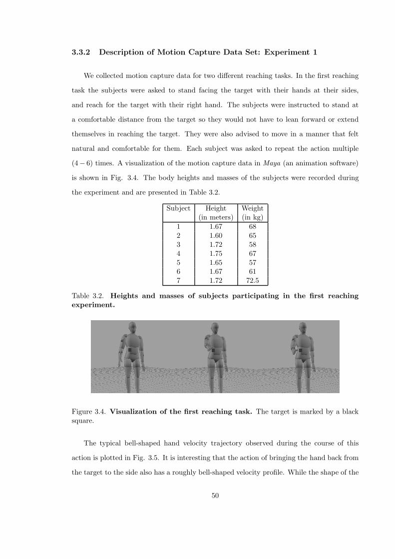
3.3.2 Description of Motion Capture Data Set: Experiment 1
We collected motion capture data for two different reaching tasks. In the first reaching
task the subjects were asked to stand facing the target with their hands at their sides,
and reach for the target with their right hand. The subjects were instructed to stand at
a comfortable distance from the target so they would not have to lean forward or extend
themselves in reaching the target. They were also advised to move in a manner that felt
natural and comfortable for them. Each subject was asked to repeat the action multiple
(4− 6) times. A visualization of the motion capture data in Maya (an animation software)
is shown in Fig. 3.4. The body heights and masses of the subjects were recorded during
the experiment and are presented in Table 3.2.
Subject Height Weight(in meters) (in kg)
1 1.67 682 1.60 653 1.72 584 1.75 675 1.65 576 1.67 617 1.72 72.5
Table 3.2. Heights and masses of subjects participating in the first reachingexperiment.
Figure 3.4. Visualization of the first reaching task. The target is marked by a blacksquare.
The typical bell-shaped hand velocity trajectory observed during the course of this
action is plotted in Fig. 3.5. It is interesting that the action of bringing the hand back from
the target to the side also has a roughly bell-shaped velocity profile. While the shape of the
50
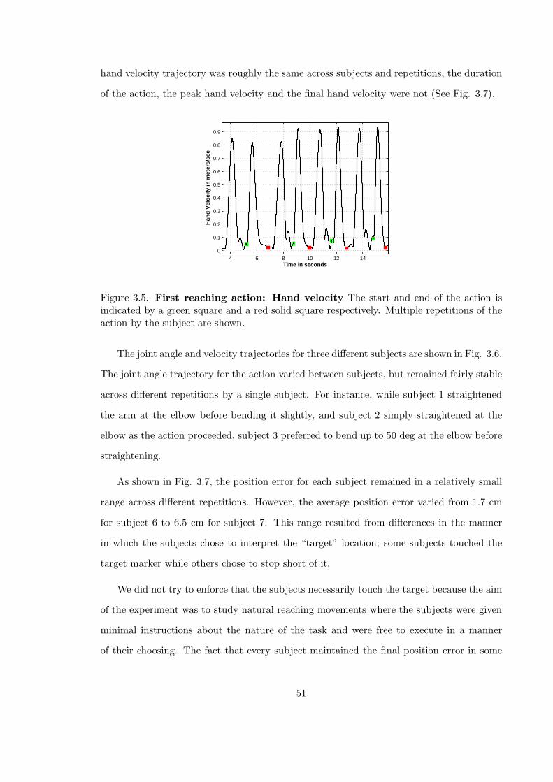
hand velocity trajectory was roughly the same across subjects and repetitions, the duration
of the action, the peak hand velocity and the final hand velocity were not (See Fig. 3.7).
4 6 8 10 12 14
0
0.1
0.2
0.3
0.4
0.5
0.6
0.7
0.8
0.9
Time in seconds
Han
d V
eloc
ity in
met
ers/
sec
Figure 3.5. First reaching action: Hand velocity The start and end of the action isindicated by a green square and a red solid square respectively. Multiple repetitions of theaction by the subject are shown.
The joint angle and velocity trajectories for three different subjects are shown in Fig. 3.6.
The joint angle trajectory for the action varied between subjects, but remained fairly stable
across different repetitions by a single subject. For instance, while subject 1 straightened
the arm at the elbow before bending it slightly, and subject 2 simply straightened at the
elbow as the action proceeded, subject 3 preferred to bend up to 50 deg at the elbow before
straightening.
As shown in Fig. 3.7, the position error for each subject remained in a relatively small
range across different repetitions. However, the average position error varied from 1.7 cm
for subject 6 to 6.5 cm for subject 7. This range resulted from differences in the manner
in which the subjects chose to interpret the “target” location; some subjects touched the
target marker while others chose to stop short of it.
We did not try to enforce that the subjects necessarily touch the target because the aim
of the experiment was to study natural reaching movements where the subjects were given
minimal instructions about the nature of the task and were free to execute in a manner
of their choosing. The fact that every subject maintained the final position error in some
51

0 0.2 0.4 0.6 0.8 1 1.2−80
−60
−40
−20
θy
degr
ees
0 0.2 0.4 0.6 0.8 1 1.270
80
90
100
θx
degr
ees
0 0.2 0.4 0.6 0.8 1 1.20
50
θe
degr
ees
Time in seconds
0 0.2 0.4 0.6 0.8 1 1.2−80−60−40−20
020
Angular velocity : θy
deg/
sec
0 0.2 0.4 0.6 0.8 1 1.2
0
20
40
θx
deg/
sec
0 0.2 0.4 0.6 0.8 1 1.2−100
0
100
θe
deg/
sec
Time in seconds
Figure 3.6. First reaching action: Joint angle and velocity trajectories for dif-ferent subjects. The joint angle and velocity trajectories for subjects 1, 2, and 3 areplotted in black, red and blue respectively. The angles correspond to the degrees of freedomdescribed in Fig. 2.1: θy and θx are the rotations about the Y and X axes, respectively, atthe shoulder joint; θe is the rotation about the elbow joint. Negative values of θy indicatethat the arm is being rotated forwards and θx = 90 deg indicates that the arm is in thesagittal plane.
limited range suggests that they maintained a consistent interpretation of the reaching task
in terms of position error. The same could not be said of the subjects’ perception of the
need to maintain a low final hand velocity. While subjects 1, 6 and 7 also consistently
controlled the final hand velocity to be at low values (Fig. 3.7), subjects 2, 3, 4 and 5 did
not.
The variations in final and peak hand velocities, and the duration of movement, even
between different repetitions of the task by the same subject, indicates the range of move-
ments associated with a single task. At the same time, the consistency of the position
error achieved by a particular subject and the invariance of hand velocity profiles across
subjects, suggests certain commonalities about how the task is executed. Our approach of
representing the reaching action by a cost function (Eq. (3.11)) captures the commonalities
of the task in the structure of the cost function, while allowing variations by allowing the
cost function parameters (wp and wv) to be varied.
52
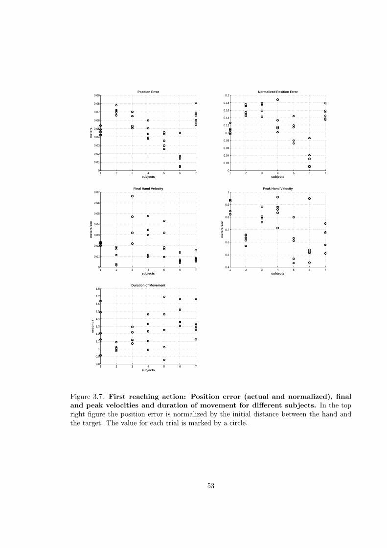
1 2 3 4 5 6 70
0.01
0.02
0.03
0.04
0.05
0.06
0.07
0.08
0.09
subjects
met
ers
Position Error
1 2 3 4 5 6 70
0.02
0.04
0.06
0.08
0.1
0.12
0.14
0.16
0.18
0.2
subjects
Normalized Position Error
1 2 3 4 5 6 70
0.01
0.02
0.03
0.04
0.05
0.06
0.07
subjects
met
ers/
sec
Final Hand Velocity
1 2 3 4 5 6 70.4
0.5
0.6
0.7
0.8
0.9
1
subjects
met
ers/
sec
Peak Hand Velocity
1 2 3 4 5 6 70.8
0.9
1
1.1
1.2
1.3
1.4
1.5
1.6
1.7
1.8
subjects
seco
nds
Duration of Movement
Figure 3.7. First reaching action: Position error (actual and normalized), finaland peak velocities and duration of movement for different subjects. In the topright figure the position error is normalized by the initial distance between the hand andthe target. The value for each trial is marked by a circle.
53
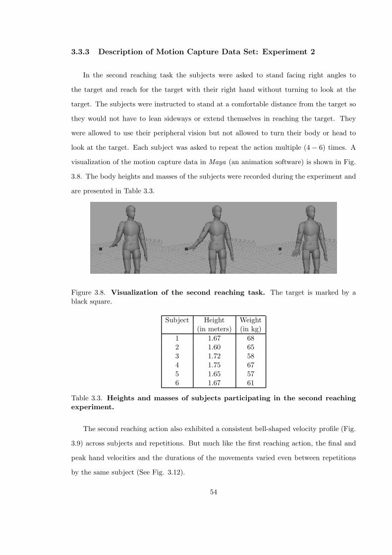
3.3.3 Description of Motion Capture Data Set: Experiment 2
In the second reaching task the subjects were asked to stand facing right angles to
the target and reach for the target with their right hand without turning to look at the
target. The subjects were instructed to stand at a comfortable distance from the target so
they would not have to lean sideways or extend themselves in reaching the target. They
were allowed to use their peripheral vision but not allowed to turn their body or head to
look at the target. Each subject was asked to repeat the action multiple (4 − 6) times. A
visualization of the motion capture data in Maya (an animation software) is shown in Fig.
3.8. The body heights and masses of the subjects were recorded during the experiment and
are presented in Table 3.3.
Figure 3.8. Visualization of the second reaching task. The target is marked by ablack square.
Subject Height Weight(in meters) (in kg)
1 1.67 682 1.60 653 1.72 584 1.75 675 1.65 576 1.67 61
Table 3.3. Heights and masses of subjects participating in the second reachingexperiment.
The second reaching action also exhibited a consistent bell-shaped velocity profile (Fig.
3.9) across subjects and repetitions. But much like the first reaching action, the final and
peak hand velocities and the durations of the movements varied even between repetitions
by the same subject (See Fig. 3.12).
54
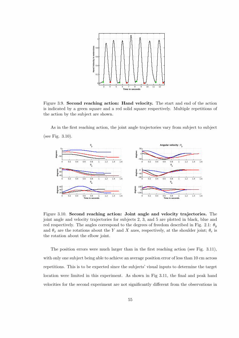
3 4 5 6 7 8 9 10 11 12
0
0.2
0.4
0.6
0.8
1
Time in seconds
Han
d V
eloc
ity in
met
ers/
sec
Figure 3.9. Second reaching action: Hand velocity. The start and end of the actionis indicated by a green square and a red solid square respectively. Multiple repetitions ofthe action by the subject are shown.
As in the first reaching action, the joint angle trajectories vary from subject to subject
(see Fig. 3.10).
0 0.2 0.4 0.6 0.8 1 1.2 1.4 1.6
−50
0
θy
degr
ees
0 0.2 0.4 0.6 0.8 1 1.2 1.4 1.6
40
60
80
θx
degr
ees
0 0.2 0.4 0.6 0.8 1 1.2 1.4 1.6
20
40
60
θe
degr
ees
Time in seconds
0 0.2 0.4 0.6 0.8 1 1.2 1.4 1.6−50
0
50
Angular velocity : θy
deg/
sec
0 0.2 0.4 0.6 0.8 1 1.2 1.4 1.6−80
−40
0
θx
deg/
sec
0 0.2 0.4 0.6 0.8 1 1.2 1.4 1.6
−100
0
100
θe
deg/
sec
Time in seconds
Figure 3.10. Second reaching action: Joint angle and velocity trajectories. Thejoint angle and velocity trajectories for subjects 2, 3, and 5 are plotted in black, blue andred respectively. The angles correspond to the degrees of freedom described in Fig. 2.1: θy
and θx are the rotations about the Y and X axes, respectively, at the shoulder joint; θe isthe rotation about the elbow joint.
The position errors were much larger than in the first reaching action (see Fig. 3.11),
with only one subject being able to achieve an average position error of less than 10 cm across
repetitions. This is to be expected since the subjects’ visual inputs to determine the target
location were limited in this experiment. As shown in Fig 3.11, the final and peak hand
velocities for the second experiment are not significantly different from the observations in
55
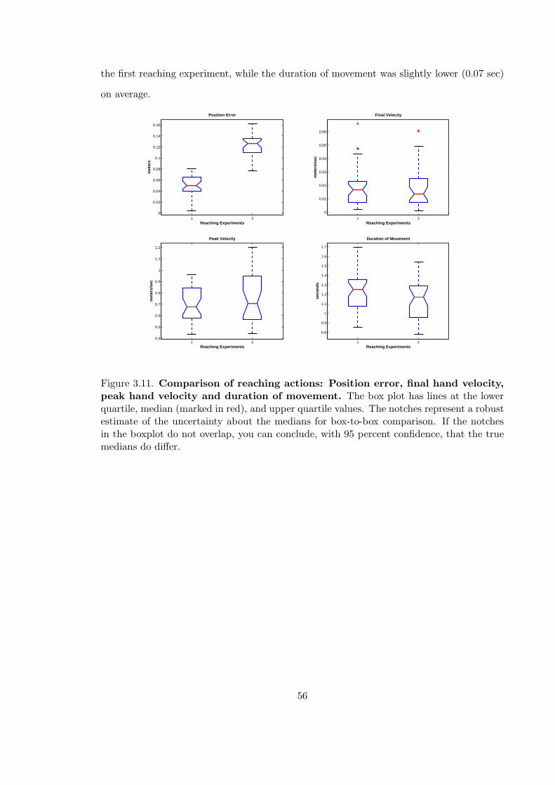
the first reaching experiment, while the duration of movement was slightly lower (0.07 sec)
on average.
1 20
0.02
0.04
0.06
0.08
0.1
0.12
0.14
0.16
met
ers
Reaching Experiments
Position Error
1 2
0
0.01
0.02
0.03
0.04
0.05
0.06
met
ers/
sec
Reaching Experiments
Final Velocity
1 20.4
0.5
0.6
0.7
0.8
0.9
1
1.1
1.2
met
ers/
sec
Reaching Experiments
Peak Velocity
1 2
0.8
0.9
1
1.1
1.2
1.3
1.4
1.5
1.6
1.7
seco
nds
Reaching Experiments
Duration of Movement
Figure 3.11. Comparison of reaching actions: Position error, final hand velocity,peak hand velocity and duration of movement. The box plot has lines at the lowerquartile, median (marked in red), and upper quartile values. The notches represent a robustestimate of the uncertainty about the medians for box-to-box comparison. If the notchesin the boxplot do not overlap, you can conclude, with 95 percent confidence, that the truemedians do differ.
56
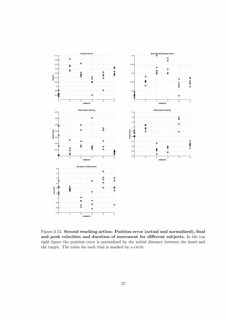
1 2 3 4 5 6
0.08
0.09
0.1
0.11
0.12
0.13
0.14
0.15
0.16
0.17
subjects
met
ers
Position Error
1 2 3 4 5 6
0.2
0.25
0.3
0.35
0.4
subjects
Normalized Position Error
1 2 3 4 5 60
0.01
0.02
0.03
0.04
0.05
0.06
0.07
subjects
met
ers/
sec
Final Hand Velocity
1 2 3 4 5 60.4
0.5
0.6
0.7
0.8
0.9
1
1.1
1.2
1.3
subjects
met
ers/
sec
Peak Hand Velocity
1 2 3 4 5 60.7
0.8
0.9
1
1.1
1.2
1.3
1.4
1.5
1.6
subjects
seco
nds
Duration of Movement
Figure 3.12. Second reaching action: Position error (actual and normalized), finaland peak velocities and duration of movement for different subjects. In the topright figure the position error is normalized by the initial distance between the hand andthe target. The value for each trial is marked by a circle.
57
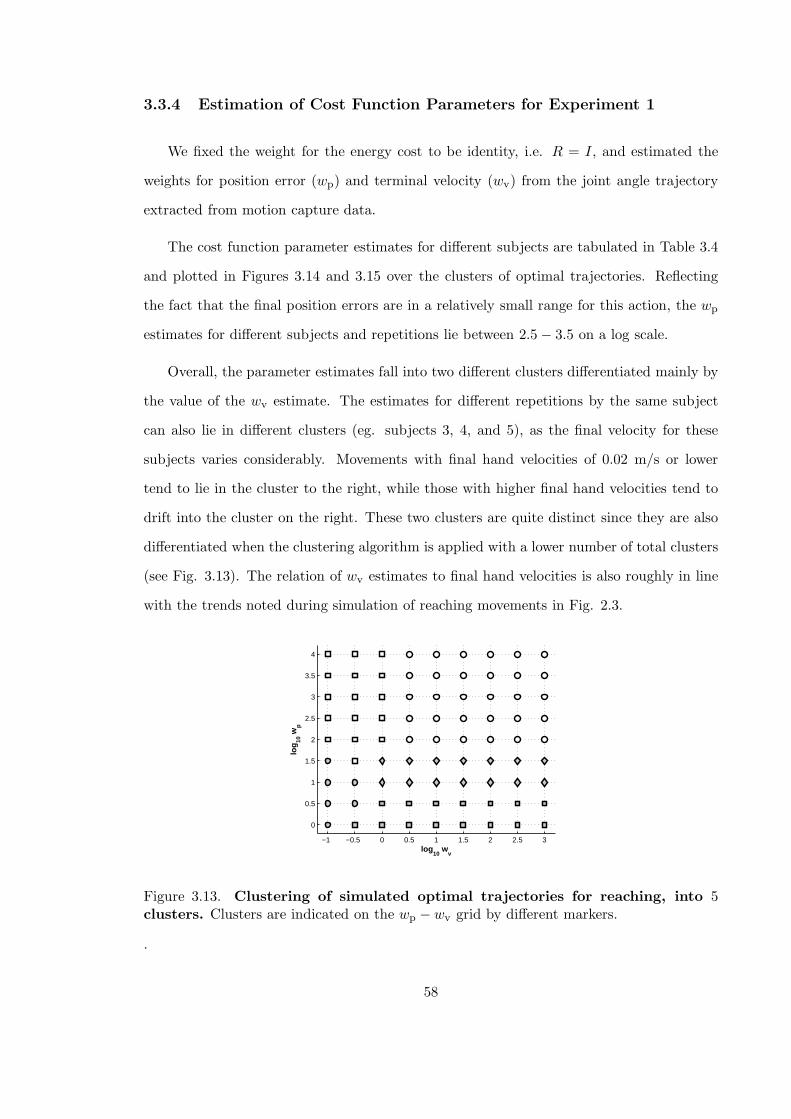
3.3.4 Estimation of Cost Function Parameters for Experiment 1
We fixed the weight for the energy cost to be identity, i.e. R = I, and estimated the
weights for position error (wp) and terminal velocity (wv) from the joint angle trajectory
extracted from motion capture data.
The cost function parameter estimates for different subjects are tabulated in Table 3.4
and plotted in Figures 3.14 and 3.15 over the clusters of optimal trajectories. Reflecting
the fact that the final position errors are in a relatively small range for this action, the wp
estimates for different subjects and repetitions lie between 2.5 − 3.5 on a log scale.
Overall, the parameter estimates fall into two different clusters differentiated mainly by
the value of the wv estimate. The estimates for different repetitions by the same subject
can also lie in different clusters (eg. subjects 3, 4, and 5), as the final velocity for these
subjects varies considerably. Movements with final hand velocities of 0.02 m/s or lower
tend to lie in the cluster to the right, while those with higher final hand velocities tend to
drift into the cluster on the right. These two clusters are quite distinct since they are also
differentiated when the clustering algorithm is applied with a lower number of total clusters
(see Fig. 3.13). The relation of wv estimates to final hand velocities is also roughly in line
with the trends noted during simulation of reaching movements in Fig. 2.3.
−1 −0.5 0 0.5 1 1.5 2 2.5 3
0
0.5
1
1.5
2
2.5
3
3.5
4
log10
wv
log
10 w
p
Figure 3.13. Clustering of simulated optimal trajectories for reaching, into 5clusters. Clusters are indicated on the wp − wv grid by different markers.
.
58

Estimates Residual Valueslog10 wp log10 wv State Costate Control Terminal
Subject 1
1 3.403 0.101 2.45e-005 0.216 0.018 6.04e-006
2 3.632 0.234 2.15e-005 0.211 0.019 6.35e-006
3 3.580 0.229 3.92e-005 0.174 0.019 6.36e-006
4 3.325 0.103 4.44e-005 0.149 0.023 4.21e-006
5 3.148 0.223 5.58e-005 0.139 0.014 3.80e-006
Subject 2
1 2.903 1.508 4.05e-005 0.139 0.056 7.03e-006
2 3.222 1.694 2.47e-005 0.116 0.092 3.53e-006
3 3.072 1.097 3.30e-005 0.132 0.063 3.51e-006
4 2.893 1.812 3.80e-005 0.132 0.071 3.57e-006
5 2.663 0.723 2.79e-005 0.131 0.094 3.83e-006
Subject 3
1 2.554 0.000 3.53e-005 0.274 0.359 1.93e-006
2 2.801 0.000 1.08e-005 0.278 0.299 4.88e-006
3 3.079 0.005 1.68e-005 0.422 0.536 3.86e-006
4 3.171 2.368 1.54e-005 0.248 0.308 3.64e-006
5 2.775 0.000 3.19e-005 0.262 0.381 4.39e-006
Subject 4
1 2.972 0.000 2.51e-005 0.239 0.201 5.52e-006
2 2.681 1.745 2.00e-005 0.226 0.300 7.71e-006
3 2.790 0.003 2.76e-005 0.301 0.321 4.28e-006
4 2.832 0.000 2.09e-005 0.331 0.364 4.78e-006
5 2.781 0.000 1.68e-005 0.271 0.294 5.17e-006
Subject 5
1 2.410 1.923 1.09e-005 0.217 0.024 1.18e-005
2 2.452 1.876 1.39e-005 0.221 0.030 1.09e-005
3 2.403 0.000 1.62e-005 0.219 0.026 1.12e-005
4 2.424 0.612 1.59e-005 0.211 0.021 1.04e-005
5 2.363 0.000 1.94e-005 0.233 0.024 8.75e-006
6 2.529 2.625 2.19e-005 0.237 0.081 9.75e-006
Subject 6
1 2.991 1.848 3.26e-005 0.158 0.042 5.23e-006
2 2.645 1.193 2.40e-005 0.135 0.051 4.83e-006
3 2.991 0.899 3.40e-005 0.136 0.068 4.11e-006
4 2.688 0.773 2.36e-005 0.124 0.030 3.74e-006
Subject 7
1 2.936 1.626 1.26e-005 0.233 0.030 8.35e-006
2 3.187 1.732 2.01e-005 0.231 0.061 6.20e-006
3 3.293 2.166 2.24e-005 0.191 0.132 4.08e-006
4 3.261 1.604 4.36e-005 0.162 0.058 9.58e-006
5 3.165 2.175 3.15e-005 0.209 0.118 7.48e-006
Table 3.4. First reaching Action: Estimates of cost function parameters.
59
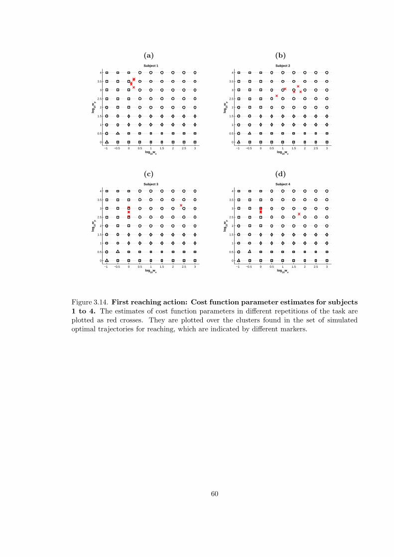
(a) (b)
−1 −0.5 0 0.5 1 1.5 2 2.5 3
0
0.5
1
1.5
2
2.5
3
3.5
4
log10
wv
log
10w
p
Subject 1
−1 −0.5 0 0.5 1 1.5 2 2.5 3
0
0.5
1
1.5
2
2.5
3
3.5
4
log10
wv
log
10w
p
Subject 2
(c) (d)
−1 −0.5 0 0.5 1 1.5 2 2.5 3
0
0.5
1
1.5
2
2.5
3
3.5
4
log10
wv
log
10w
p
Subject 3
−1 −0.5 0 0.5 1 1.5 2 2.5 3
0
0.5
1
1.5
2
2.5
3
3.5
4
log10
wv
log
10w
p
Subject 4
Figure 3.14. First reaching action: Cost function parameter estimates for subjects1 to 4. The estimates of cost function parameters in different repetitions of the task areplotted as red crosses. They are plotted over the clusters found in the set of simulatedoptimal trajectories for reaching, which are indicated by different markers.
60
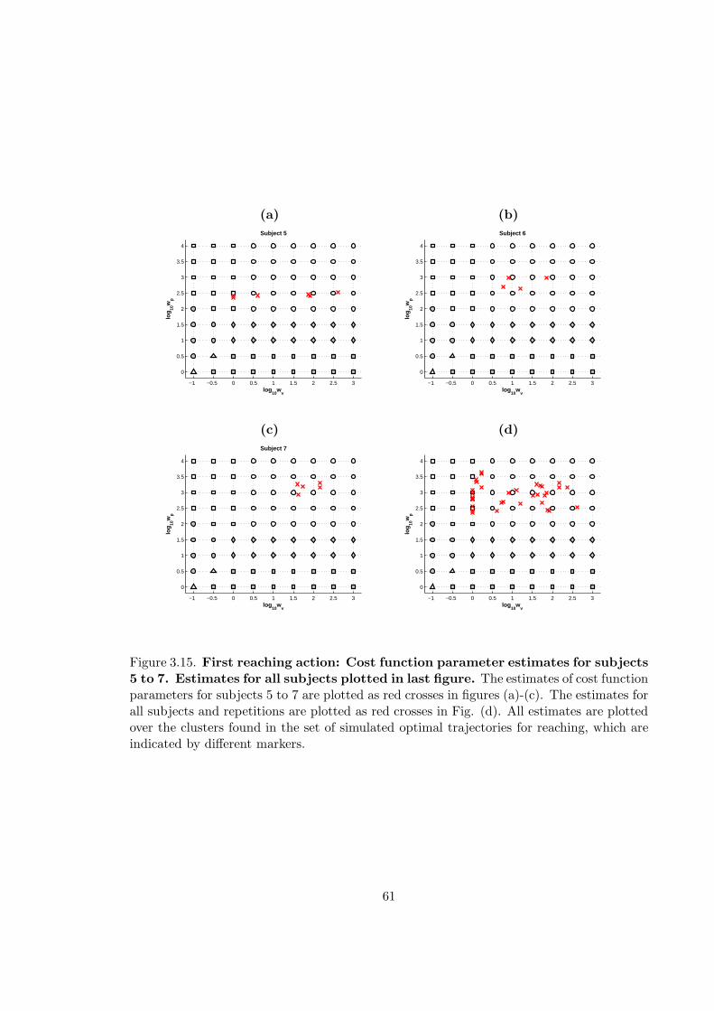
(a) (b)
−1 −0.5 0 0.5 1 1.5 2 2.5 3
0
0.5
1
1.5
2
2.5
3
3.5
4
log10
wv
log
10w
p
Subject 5
−1 −0.5 0 0.5 1 1.5 2 2.5 3
0
0.5
1
1.5
2
2.5
3
3.5
4
log10
wv
log
10w
p
Subject 6
(c) (d)
−1 −0.5 0 0.5 1 1.5 2 2.5 3
0
0.5
1
1.5
2
2.5
3
3.5
4
log10
wv
log
10w
p
Subject 7
−1 −0.5 0 0.5 1 1.5 2 2.5 3
0
0.5
1
1.5
2
2.5
3
3.5
4
log10
wv
log
10w
p
Figure 3.15. First reaching action: Cost function parameter estimates for subjects5 to 7. Estimates for all subjects plotted in last figure. The estimates of cost functionparameters for subjects 5 to 7 are plotted as red crosses in figures (a)-(c). The estimates forall subjects and repetitions are plotted as red crosses in Fig. (d). All estimates are plottedover the clusters found in the set of simulated optimal trajectories for reaching, which areindicated by different markers.
61
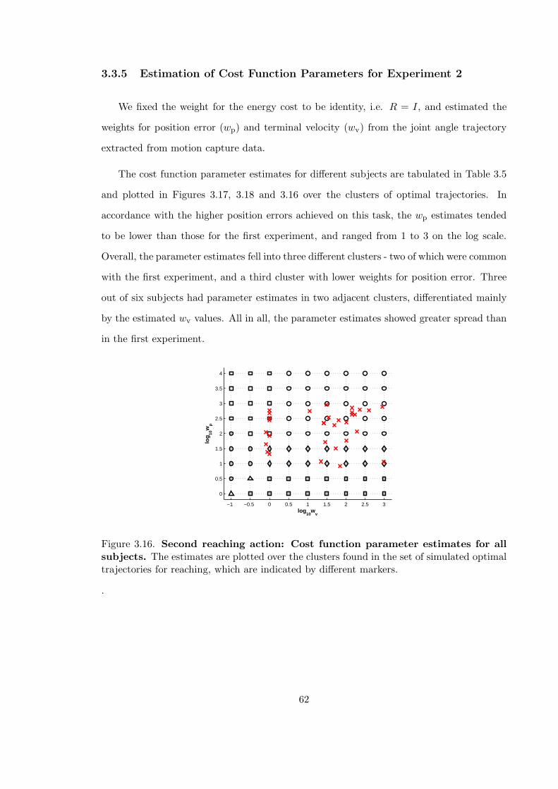
3.3.5 Estimation of Cost Function Parameters for Experiment 2
We fixed the weight for the energy cost to be identity, i.e. R = I, and estimated the
weights for position error (wp) and terminal velocity (wv) from the joint angle trajectory
extracted from motion capture data.
The cost function parameter estimates for different subjects are tabulated in Table 3.5
and plotted in Figures 3.17, 3.18 and 3.16 over the clusters of optimal trajectories. In
accordance with the higher position errors achieved on this task, the wp estimates tended
to be lower than those for the first experiment, and ranged from 1 to 3 on the log scale.
Overall, the parameter estimates fell into three different clusters - two of which were common
with the first experiment, and a third cluster with lower weights for position error. Three
out of six subjects had parameter estimates in two adjacent clusters, differentiated mainly
by the estimated wv values. All in all, the parameter estimates showed greater spread than
in the first experiment.
−1 −0.5 0 0.5 1 1.5 2 2.5 3
0
0.5
1
1.5
2
2.5
3
3.5
4
log10
wv
log
10w
p
Figure 3.16. Second reaching action: Cost function parameter estimates for allsubjects. The estimates are plotted over the clusters found in the set of simulated optimaltrajectories for reaching, which are indicated by different markers.
.
62
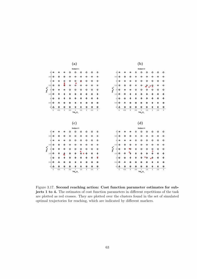
(a) (b)
−1 −0.5 0 0.5 1 1.5 2 2.5 3
0
0.5
1
1.5
2
2.5
3
3.5
4
log10
wv
log
10w
p
Subject 1
−1 −0.5 0 0.5 1 1.5 2 2.5 3
0
0.5
1
1.5
2
2.5
3
3.5
4
log10
wv
log
10w
p
Subject 2
(c) (d)
−1 −0.5 0 0.5 1 1.5 2 2.5 3
0
0.5
1
1.5
2
2.5
3
3.5
4
log10
wv
log
10w
p
Subject 3
−1 −0.5 0 0.5 1 1.5 2 2.5 3
0
0.5
1
1.5
2
2.5
3
3.5
4
log10
wv
log
10w
p
Subject 4
Figure 3.17. Second reaching action: Cost function parameter estimates for sub-jects 1 to 4. The estimates of cost function parameters in different repetitions of the taskare plotted as red crosses. They are plotted over the clusters found in the set of simulatedoptimal trajectories for reaching, which are indicated by different markers.
63
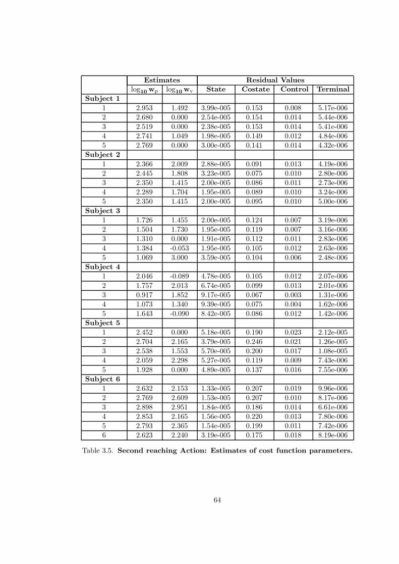
Estimates Residual Valueslog10 wp log10 wv State Costate Control Terminal
Subject 1
1 2.953 1.492 3.99e-005 0.153 0.008 5.17e-006
2 2.680 0.000 2.54e-005 0.154 0.014 5.44e-006
3 2.519 0.000 2.38e-005 0.153 0.014 5.41e-006
4 2.741 1.049 1.98e-005 0.149 0.012 4.84e-006
5 2.769 0.000 3.00e-005 0.141 0.014 4.32e-006
Subject 2
1 2.366 2.009 2.88e-005 0.091 0.013 4.19e-006
2 2.445 1.808 3.23e-005 0.075 0.010 2.80e-006
3 2.350 1.415 2.00e-005 0.086 0.011 2.73e-006
4 2.289 1.704 1.95e-005 0.089 0.010 3.24e-006
5 2.350 1.415 2.00e-005 0.095 0.010 5.00e-006
Subject 3
1 1.726 1.455 2.00e-005 0.124 0.007 3.19e-006
2 1.504 1.730 1.95e-005 0.119 0.007 3.16e-006
3 1.310 0.000 1.91e-005 0.112 0.011 2.83e-006
4 1.384 -0.053 1.95e-005 0.105 0.012 2.63e-006
5 1.069 3.000 3.59e-005 0.104 0.006 2.48e-006
Subject 4
1 2.046 -0.089 4.78e-005 0.105 0.012 2.07e-006
2 1.757 2.013 6.74e-005 0.099 0.013 2.01e-006
3 0.917 1.852 9.17e-005 0.067 0.003 1.31e-006
4 1.073 1.340 9.39e-005 0.075 0.004 1.62e-006
5 1.643 -0.090 8.42e-005 0.086 0.012 1.42e-006
Subject 5
1 2.452 0.000 5.18e-005 0.190 0.023 2.12e-005
2 2.704 2.165 3.79e-005 0.246 0.021 1.26e-005
3 2.538 1.553 5.70e-005 0.200 0.017 1.08e-005
4 2.059 2.298 5.27e-005 0.119 0.009 7.43e-006
5 1.928 0.000 4.89e-005 0.137 0.016 7.55e-006
Subject 6
1 2.632 2.153 1.33e-005 0.207 0.019 9.96e-006
2 2.769 2.609 1.53e-005 0.207 0.010 8.17e-006
3 2.898 2.951 1.84e-005 0.186 0.014 6.61e-006
4 2.853 2.165 1.56e-005 0.220 0.013 7.80e-006
5 2.793 2.365 1.54e-005 0.199 0.011 7.42e-006
6 2.623 2.240 3.19e-005 0.175 0.018 8.19e-006
Table 3.5. Second reaching Action: Estimates of cost function parameters.
64
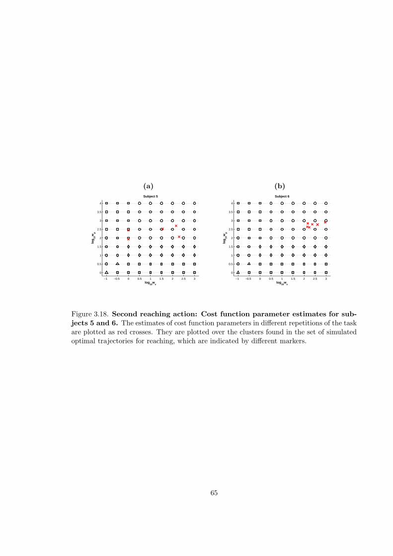
(a) (b)
−1 −0.5 0 0.5 1 1.5 2 2.5 3
0
0.5
1
1.5
2
2.5
3
3.5
4
log10
wv
log
10w
p
Subject 5
−1 −0.5 0 0.5 1 1.5 2 2.5 3
0
0.5
1
1.5
2
2.5
3
3.5
4
log10
wv
log
10w
p
Subject 6
Figure 3.18. Second reaching action: Cost function parameter estimates for sub-jects 5 and 6. The estimates of cost function parameters in different repetitions of the taskare plotted as red crosses. They are plotted over the clusters found in the set of simulatedoptimal trajectories for reaching, which are indicated by different markers.
65
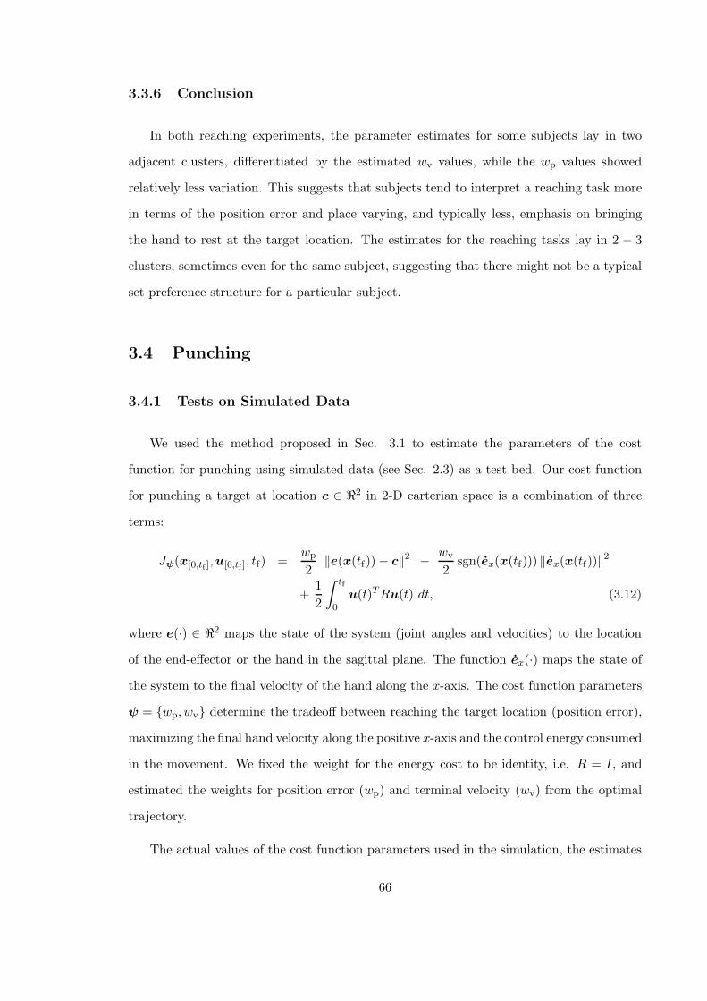
3.3.6 Conclusion
In both reaching experiments, the parameter estimates for some subjects lay in two
adjacent clusters, differentiated by the estimated wv values, while the wp values showed
relatively less variation. This suggests that subjects tend to interpret a reaching task more
in terms of the position error and place varying, and typically less, emphasis on bringing
the hand to rest at the target location. The estimates for the reaching tasks lay in 2 − 3
clusters, sometimes even for the same subject, suggesting that there might not be a typical
set preference structure for a particular subject.
3.4 Punching
3.4.1 Tests on Simulated Data
We used the method proposed in Sec. 3.1 to estimate the parameters of the cost
function for punching using simulated data (see Sec. 2.3) as a test bed. Our cost function
for punching a target at location c ∈ ℜ2 in 2-D carterian space is a combination of three
terms:
Jψ(x[0,tf ],u[0,tf ], tf) =wp
2‖e(x(tf)) − c‖
2 −wv
2sgn(ex(x(tf))) ‖ex(x(tf))‖
2
+1
2
∫ tf
0u(t)T Ru(t) dt, (3.12)
where e(·) ∈ ℜ2 maps the state of the system (joint angles and velocities) to the location
of the end-effector or the hand in the sagittal plane. The function ex(·) maps the state of
the system to the final velocity of the hand along the x-axis. The cost function parameters
ψ = {wp, wv} determine the tradeoff between reaching the target location (position error),
maximizing the final hand velocity along the positive x-axis and the control energy consumed
in the movement. We fixed the weight for the energy cost to be identity, i.e. R = I, and
estimated the weights for position error (wp) and terminal velocity (wv) from the optimal
trajectory.
The actual values of the cost function parameters used in the simulation, the estimates
66
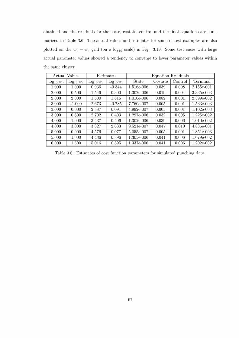
obtained and the residuals for the state, costate, control and terminal equations are sum-
marized in Table 3.6. The actual values and estimates for some of test examples are also
plotted on the wp − wv grid (on a log10 scale) in Fig. 3.19. Some test cases with large
actual parameter values showed a tendency to converge to lower parameter values within
the same cluster.
Actual Values Estimates Equation Residuals
log10 wp log10 wv log10 wp log10 wv State Costate Control Terminal
1.000 1.000 0.936 -0.344 1.516e-006 0.039 0.008 2.155e-001
2.000 0.500 1.546 0.300 1.302e-006 0.019 0.004 3.335e-003
2.000 2.000 1.500 1.816 1.010e-006 0.082 0.001 2.399e-002
3.000 -1.000 2.673 -0.785 7.760e-007 0.005 0.001 1.533e-003
3.000 0.000 2.587 0.091 4.992e-007 0.005 0.001 1.102e-003
3.000 0.500 2.702 0.403 1.297e-006 0.032 0.005 1.225e-002
4.000 1.000 3.437 0.406 1.302e-006 0.039 0.006 1.010e-002
4.000 3.000 3.827 2.633 9.521e-007 0.047 0.010 4.886e-001
5.000 0.000 4.576 0.077 5.055e-007 0.005 0.001 1.351e-003
5.000 1.000 4.436 0.396 1.305e-006 0.041 0.006 1.079e-002
6.000 1.500 5.016 0.395 1.337e-006 0.041 0.006 1.202e-002
Table 3.6. Estimates of cost function parameters for simulated punching data.
67
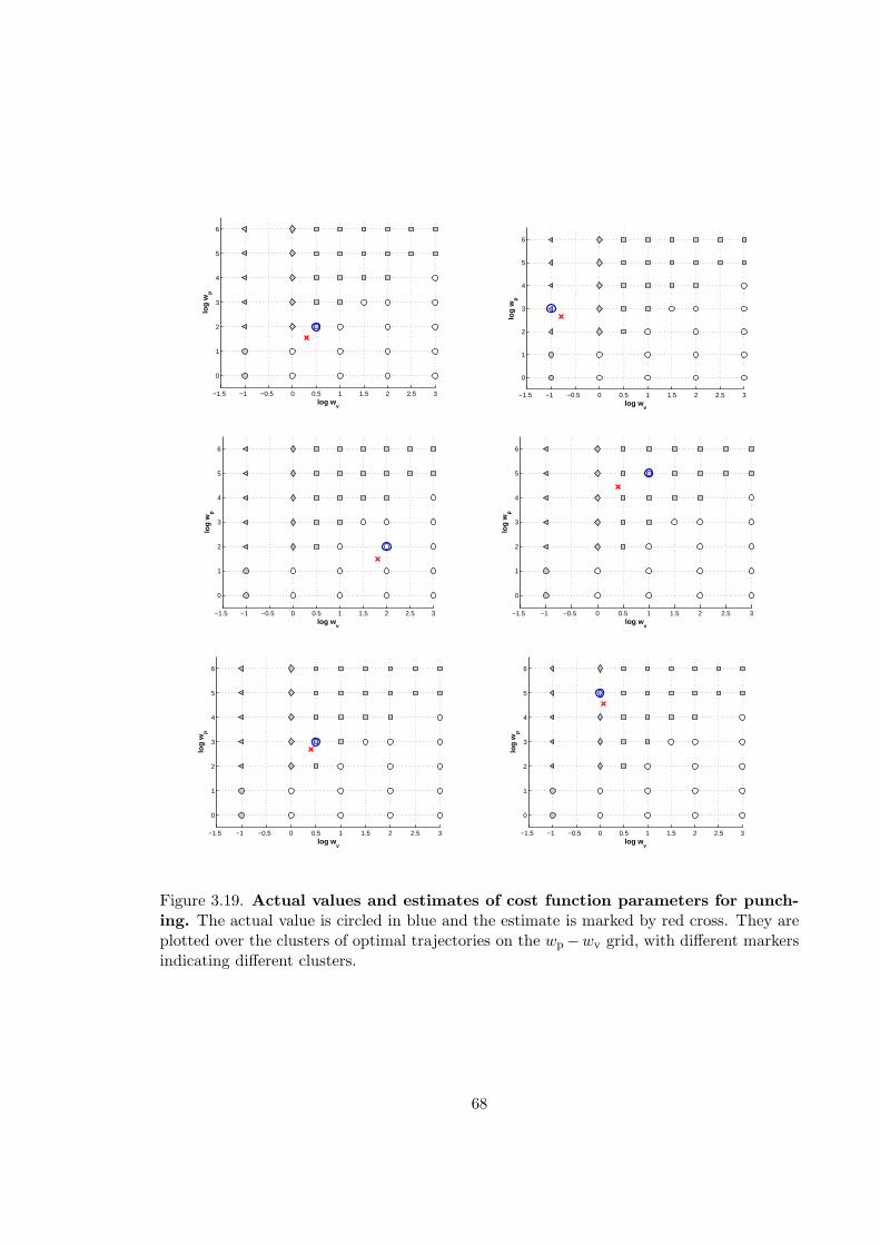
−1.5 −1 −0.5 0 0.5 1 1.5 2 2.5 3
0
1
2
3
4
5
6
log wv
log
wp
−1.5 −1 −0.5 0 0.5 1 1.5 2 2.5 3
0
1
2
3
4
5
6
log wv
log
wp
−1.5 −1 −0.5 0 0.5 1 1.5 2 2.5 3
0
1
2
3
4
5
6
log wv
log
wp
−1.5 −1 −0.5 0 0.5 1 1.5 2 2.5 3
0
1
2
3
4
5
6
log wv
log
wp
−1.5 −1 −0.5 0 0.5 1 1.5 2 2.5 3
0
1
2
3
4
5
6
log wv
log
wp
−1.5 −1 −0.5 0 0.5 1 1.5 2 2.5 3
0
1
2
3
4
5
6
log wv
log
wp
Figure 3.19. Actual values and estimates of cost function parameters for punch-ing. The actual value is circled in blue and the estimate is marked by red cross. They areplotted over the clusters of optimal trajectories on the wp −wv grid, with different markersindicating different clusters.
68
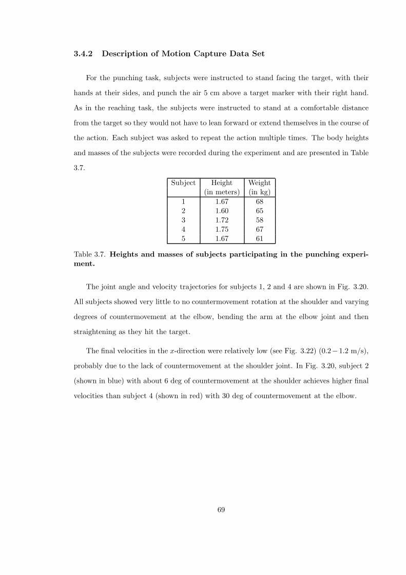
3.4.2 Description of Motion Capture Data Set
For the punching task, subjects were instructed to stand facing the target, with their
hands at their sides, and punch the air 5 cm above a target marker with their right hand.
As in the reaching task, the subjects were instructed to stand at a comfortable distance
from the target so they would not have to lean forward or extend themselves in the course of
the action. Each subject was asked to repeat the action multiple times. The body heights
and masses of the subjects were recorded during the experiment and are presented in Table
3.7.
Subject Height Weight(in meters) (in kg)
1 1.67 682 1.60 653 1.72 584 1.75 675 1.67 61
Table 3.7. Heights and masses of subjects participating in the punching experi-ment.
The joint angle and velocity trajectories for subjects 1, 2 and 4 are shown in Fig. 3.20.
All subjects showed very little to no countermovement rotation at the shoulder and varying
degrees of countermovement at the elbow, bending the arm at the elbow joint and then
straightening as they hit the target.
The final velocities in the x-direction were relatively low (see Fig. 3.22) (0.2−1.2 m/s),
probably due to the lack of countermovement at the shoulder joint. In Fig. 3.20, subject 2
(shown in blue) with about 6 deg of countermovement at the shoulder achieves higher final
velocities than subject 4 (shown in red) with 30 deg of countermovement at the elbow.
69
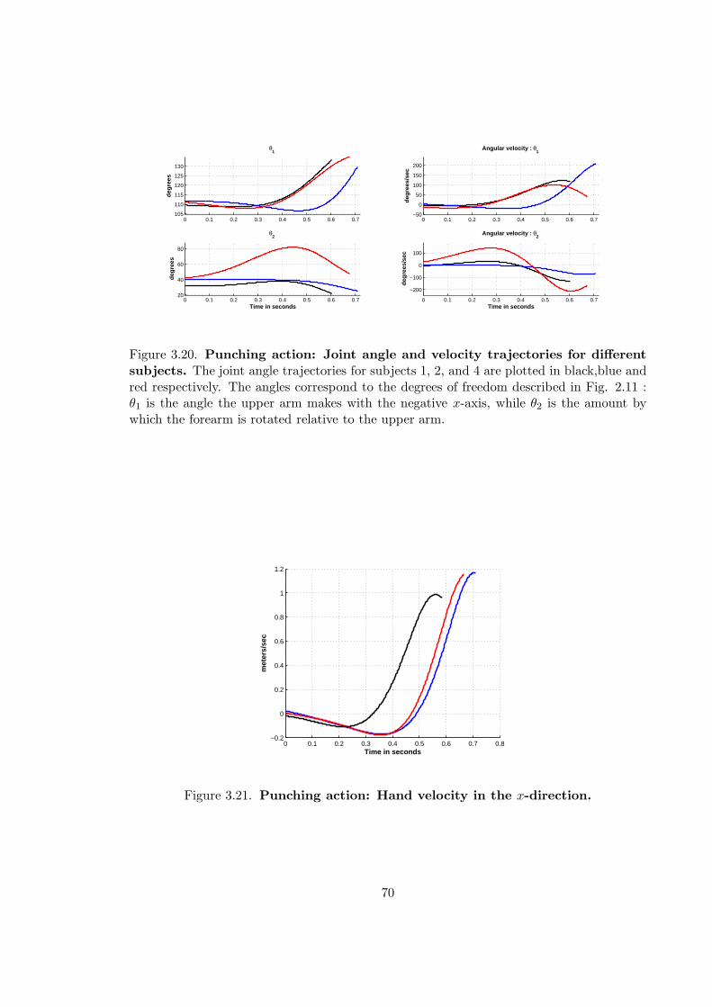
0 0.1 0.2 0.3 0.4 0.5 0.6 0.7105
110
115
120
125
130
θ1
degr
ees
0 0.1 0.2 0.3 0.4 0.5 0.6 0.720
40
60
80
θ2
degr
ees
Time in seconds
0 0.1 0.2 0.3 0.4 0.5 0.6 0.7−50
0
50
100
150
200
Angular velocity : θ1
degr
ees/
sec
0 0.1 0.2 0.3 0.4 0.5 0.6 0.7
−200
−100
0
100
Angular velocity : θ2
degr
ees/
sec
Time in seconds
Figure 3.20. Punching action: Joint angle and velocity trajectories for differentsubjects. The joint angle trajectories for subjects 1, 2, and 4 are plotted in black,blue andred respectively. The angles correspond to the degrees of freedom described in Fig. 2.11 :θ1 is the angle the upper arm makes with the negative x-axis, while θ2 is the amount bywhich the forearm is rotated relative to the upper arm.
0 0.1 0.2 0.3 0.4 0.5 0.6 0.7 0.8−0.2
0
0.2
0.4
0.6
0.8
1
1.2
Time in seconds
met
ers/
sec
Figure 3.21. Punching action: Hand velocity in the x-direction.
70
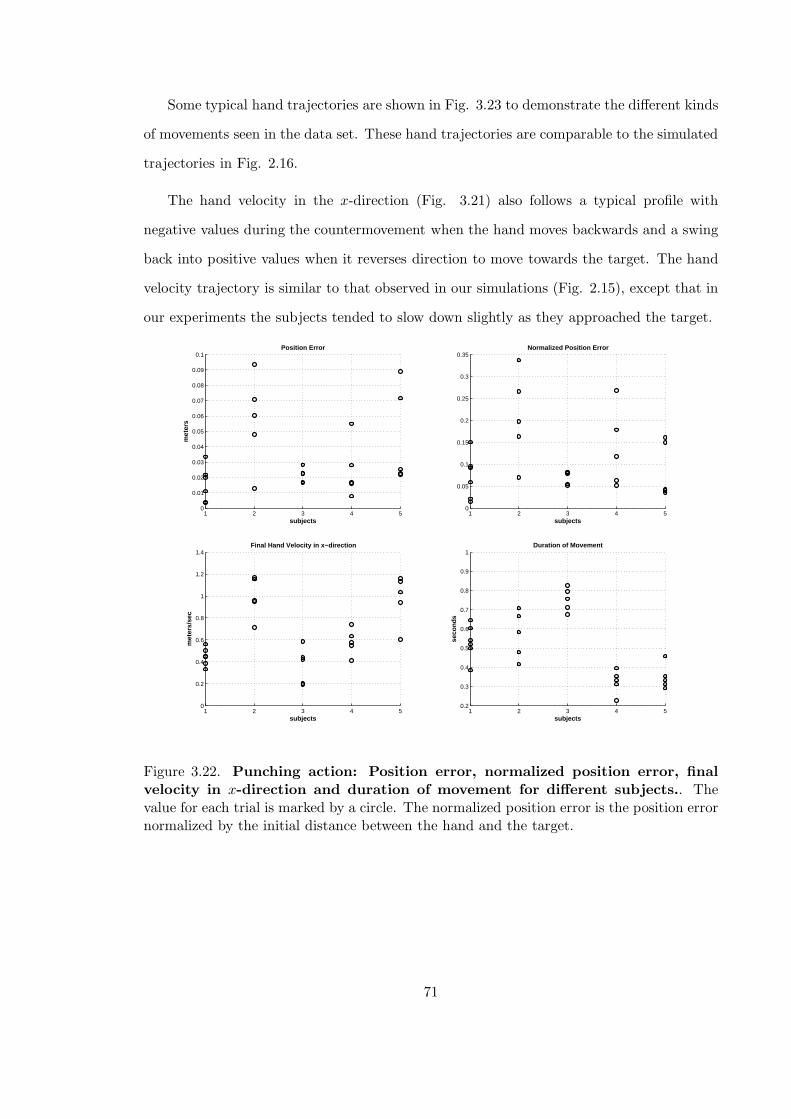
Some typical hand trajectories are shown in Fig. 3.23 to demonstrate the different kinds
of movements seen in the data set. These hand trajectories are comparable to the simulated
trajectories in Fig. 2.16.
The hand velocity in the x-direction (Fig. 3.21) also follows a typical profile with
negative values during the countermovement when the hand moves backwards and a swing
back into positive values when it reverses direction to move towards the target. The hand
velocity trajectory is similar to that observed in our simulations (Fig. 2.15), except that in
our experiments the subjects tended to slow down slightly as they approached the target.
1 2 3 4 50
0.01
0.02
0.03
0.04
0.05
0.06
0.07
0.08
0.09
0.1
subjects
met
ers
Position Error
1 2 3 4 50
0.05
0.1
0.15
0.2
0.25
0.3
0.35
subjects
Normalized Position Error
1 2 3 4 50
0.2
0.4
0.6
0.8
1
1.2
1.4
subjects
met
ers/
sec
Final Hand Velocity in x−direction
1 2 3 4 50.2
0.3
0.4
0.5
0.6
0.7
0.8
0.9
1
subjects
seco
nds
Duration of Movement
Figure 3.22. Punching action: Position error, normalized position error, finalvelocity in x-direction and duration of movement for different subjects.. Thevalue for each trial is marked by a circle. The normalized position error is the position errornormalized by the initial distance between the hand and the target.
71
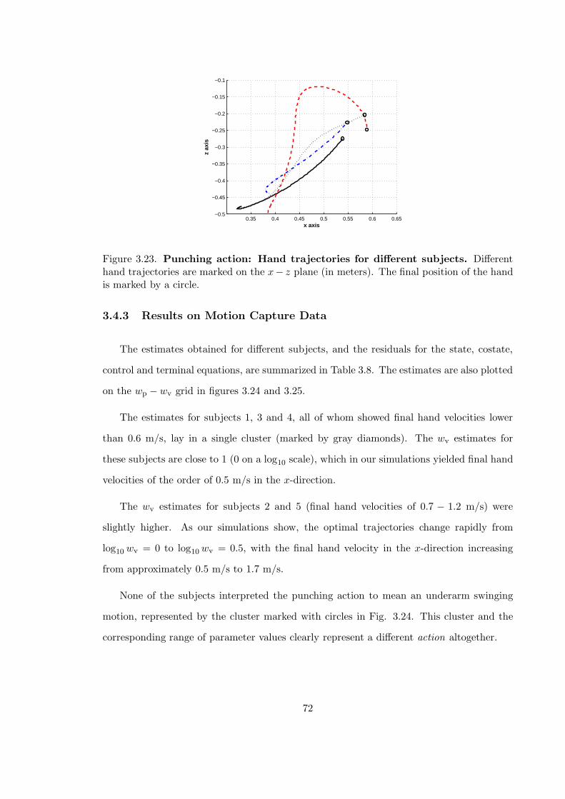
0.35 0.4 0.45 0.5 0.55 0.6 0.65−0.5
−0.45
−0.4
−0.35
−0.3
−0.25
−0.2
−0.15
−0.1
x axis
z ax
is
Figure 3.23. Punching action: Hand trajectories for different subjects. Differenthand trajectories are marked on the x− z plane (in meters). The final position of the handis marked by a circle.
3.4.3 Results on Motion Capture Data
The estimates obtained for different subjects, and the residuals for the state, costate,
control and terminal equations, are summarized in Table 3.8. The estimates are also plotted
on the wp − wv grid in figures 3.24 and 3.25.
The estimates for subjects 1, 3 and 4, all of whom showed final hand velocities lower
than 0.6 m/s, lay in a single cluster (marked by gray diamonds). The wv estimates for
these subjects are close to 1 (0 on a log10 scale), which in our simulations yielded final hand
velocities of the order of 0.5 m/s in the x-direction.
The wv estimates for subjects 2 and 5 (final hand velocities of 0.7 − 1.2 m/s) were
slightly higher. As our simulations show, the optimal trajectories change rapidly from
log10 wv = 0 to log10 wv = 0.5, with the final hand velocity in the x-direction increasing
from approximately 0.5 m/s to 1.7 m/s.
None of the subjects interpreted the punching action to mean an underarm swinging
motion, represented by the cluster marked with circles in Fig. 3.24. This cluster and the
corresponding range of parameter values clearly represent a different action altogether.
72

(a) (b)
−1 0 1 2 3 4 5 6
0
1
2
3
4
5
6
log wv
log
wp
Subject 1
−1 0 1 2 3 4 5 6
0
1
2
3
4
5
6
log wv
log
wp
Subject 2
(c) (d)
−1 0 1 2 3 4 5 6
0
1
2
3
4
5
6
log wv
log
wp
Subject 3
−1 0 1 2 3 4 5 6
0
1
2
3
4
5
6
log wv
log
wp
Subject 4
Figure 3.24. Punching action: Cost function parameter estimates for subjects 1to 4. The estimates of cost function parameters for subjects 1 to 4 are plotted as red crossesin figures (a)-(d). All estimates are plotted over the clusters found in the set of simulatedoptimal trajectories for punching, which are indicated by different markers.
73
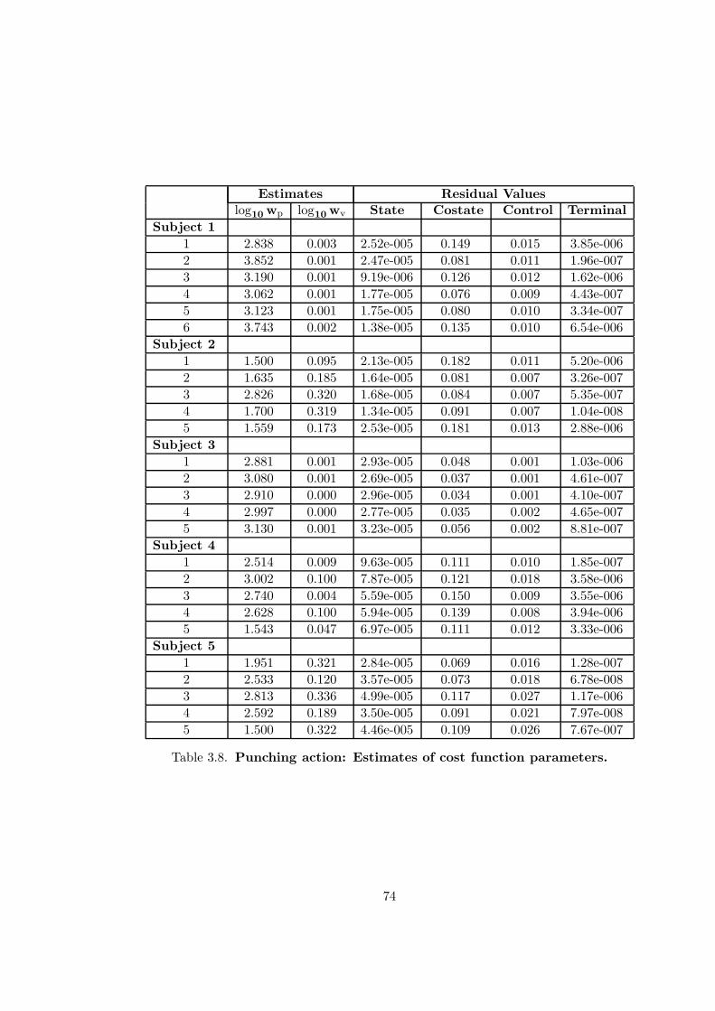
Estimates Residual Valueslog10 wp log10 wv State Costate Control Terminal
Subject 1
1 2.838 0.003 2.52e-005 0.149 0.015 3.85e-006
2 3.852 0.001 2.47e-005 0.081 0.011 1.96e-007
3 3.190 0.001 9.19e-006 0.126 0.012 1.62e-006
4 3.062 0.001 1.77e-005 0.076 0.009 4.43e-007
5 3.123 0.001 1.75e-005 0.080 0.010 3.34e-007
6 3.743 0.002 1.38e-005 0.135 0.010 6.54e-006
Subject 2
1 1.500 0.095 2.13e-005 0.182 0.011 5.20e-006
2 1.635 0.185 1.64e-005 0.081 0.007 3.26e-007
3 2.826 0.320 1.68e-005 0.084 0.007 5.35e-007
4 1.700 0.319 1.34e-005 0.091 0.007 1.04e-008
5 1.559 0.173 2.53e-005 0.181 0.013 2.88e-006
Subject 3
1 2.881 0.001 2.93e-005 0.048 0.001 1.03e-006
2 3.080 0.001 2.69e-005 0.037 0.001 4.61e-007
3 2.910 0.000 2.96e-005 0.034 0.001 4.10e-007
4 2.997 0.000 2.77e-005 0.035 0.002 4.65e-007
5 3.130 0.001 3.23e-005 0.056 0.002 8.81e-007
Subject 4
1 2.514 0.009 9.63e-005 0.111 0.010 1.85e-007
2 3.002 0.100 7.87e-005 0.121 0.018 3.58e-006
3 2.740 0.004 5.59e-005 0.150 0.009 3.55e-006
4 2.628 0.100 5.94e-005 0.139 0.008 3.94e-006
5 1.543 0.047 6.97e-005 0.111 0.012 3.33e-006
Subject 5
1 1.951 0.321 2.84e-005 0.069 0.016 1.28e-007
2 2.533 0.120 3.57e-005 0.073 0.018 6.78e-008
3 2.813 0.336 4.99e-005 0.117 0.027 1.17e-006
4 2.592 0.189 3.50e-005 0.091 0.021 7.97e-008
5 1.500 0.322 4.46e-005 0.109 0.026 7.67e-007
Table 3.8. Punching action: Estimates of cost function parameters.
74
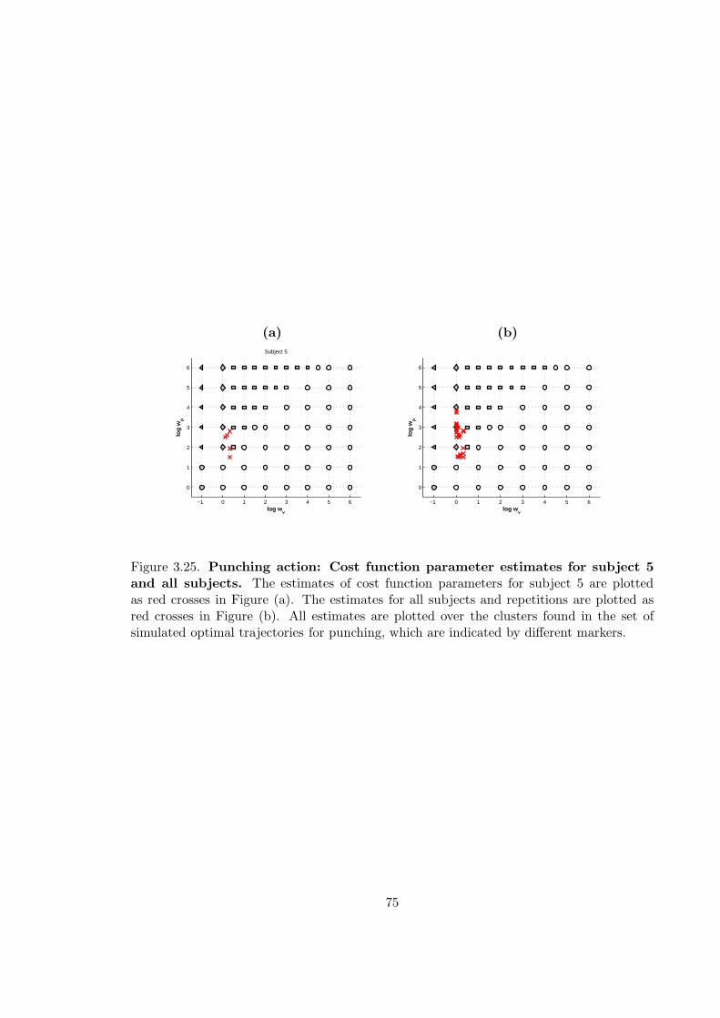
(a) (b)
−1 0 1 2 3 4 5 6
0
1
2
3
4
5
6
log wv
log
wp
Subject 5
−1 0 1 2 3 4 5 6
0
1
2
3
4
5
6
log wv
log
wp
Figure 3.25. Punching action: Cost function parameter estimates for subject 5and all subjects. The estimates of cost function parameters for subject 5 are plottedas red crosses in Figure (a). The estimates for all subjects and repetitions are plotted asred crosses in Figure (b). All estimates are plotted over the clusters found in the set ofsimulated optimal trajectories for punching, which are indicated by different markers.
75
Chapter 4
Recognition in an Optimal Control
Framework
Recognition of human actions is an important application that any representation of
human actions should be able to address. In this section we demonstrate how different
actions can be recognized and segmented within the framework of optimal control that we
outlined in the previous chapters.
Different cost functions, corresponding to different goal-directed tasks, are the basic
building blocks in our representation. The cost function captures two levels of detail about
the action: the goal of the action or what the person is doing, and the preferences expressed
in the execution of the action or how the person is executing the action. The goal of the
action is encoded in the structure of the cost function, while the preferences are captured
by the cost function parameters or weights.
In the previous chapters we focussed on a single cost function structure at a time and
estimated from observations the preferences, that is the cost function parameters. We found
that while the preferences varied even between different repetitions of the task by a single
subject, overall there were only 2-3 significantly different clusters of preferences for the arm
movements we studied. This suggests that for these movements 2-3 cost function primitives
could be constructed to capture the variation.
76
While in the previous chapter we were focussed on teasing apart the differences in how
subjects performed the same task, in this section we shall focus on segmenting different tasks
i.e. movements that correspond to different cost functions. Let us assume that we are given
a library of cost functions corresponding to the different tasks we wish to recognize and
segment from a stream of observations. The parameters of these cost functions are fixed,
estimated by methods described in the previous chapter. We refer to the cost functions in
this library as cost function primitives.
We view the human motor system as a hybrid system that switches between different
cost function primitives, in response to changing high-level goals. The problem of action
recognition is to infer the hidden goal of the motion from the observed movement trajectory.
Complex actions can be modeled as the comsposition of simpler goals. For example, the
goal of lifting an object can be viewed as the composition of two goal-directed actions -
reaching for it and then lifting it.
4.1 Models
Given noisy kinematic observations of a motion (eg. 3D hand trajectory for an arm mo-
tion), we wish to estimate the underlying sequence of cost function primitives that produced
the motion. Thus there are four different variables in our model : a discrete mode variable
mk which indicates which of the cost function primitives is active at the k-th instant, a
state vector xk of joint angles and velocities, a control vector uk of joint torques, and an
observation vector yk. The dependencies between these variables are shown in the form of
a graphical model in Fig. 4.1.
We assume that the observations yk available to us are of the form
yk = g(xk) + nk, (4.1)
where the function g(·) is known to us and the noise nk is i.i.d. zero mean Gaussian with
known covariance Σn.
We also assume that all the cost function primitives (modes) in the library are equally
77
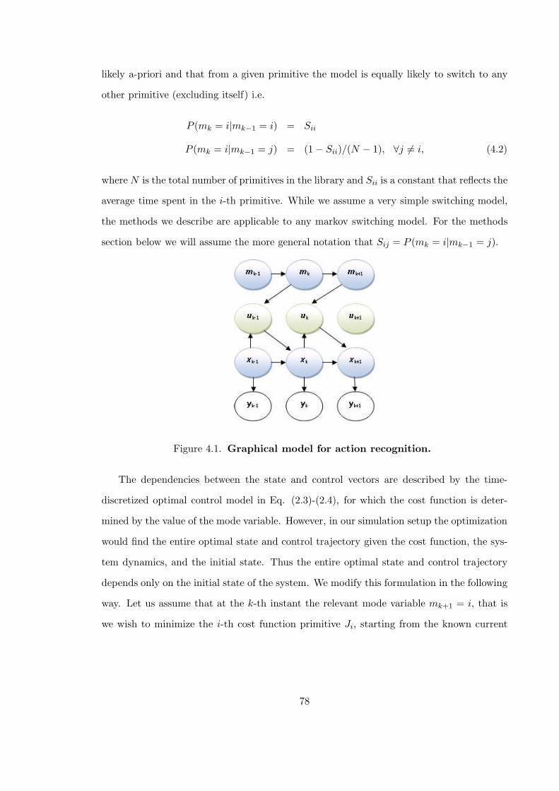
likely a-priori and that from a given primitive the model is equally likely to switch to any
other primitive (excluding itself) i.e.
P (mk = i|mk−1 = i) = Sii
P (mk = i|mk−1 = j) = (1 − Sii)/(N − 1), ∀j 6= i, (4.2)
where N is the total number of primitives in the library and Sii is a constant that reflects the
average time spent in the i-th primitive. While we assume a very simple switching model,
the methods we describe are applicable to any markov switching model. For the methods
section below we will assume the more general notation that Sij = P (mk = i|mk−1 = j).
Figure 4.1. Graphical model for action recognition.
The dependencies between the state and control vectors are described by the time-
discretized optimal control model in Eq. (2.3)-(2.4), for which the cost function is deter-
mined by the value of the mode variable. However, in our simulation setup the optimization
would find the entire optimal state and control trajectory given the cost function, the sys-
tem dynamics, and the initial state. Thus the entire optimal state and control trajectory
depends only on the initial state of the system. We modify this formulation in the following
way. Let us assume that at the k-th instant the relevant mode variable mk+1 = i, that is
we wish to minimize the i-th cost function primitive Ji, starting from the known current
78
state of the system xk. We solve the free-final time optimal control problem
minxk+1,...,xk+M−1,uk,...,uk+M−1,tf
Ji(xk+1, . . . ,xk+M−1,uk, . . . ,uk+M−1, tf)
s.t. xt − xt−1 −−∆
2(f(xt,ut) + f(xt−1,ut−1)) = 0
t = k + 1, . . . , k + M − 1. (4.3)
where M is fixed and can be chosen to ensure that the discretization interval ∆ = tf/(M−1)
is sufficiently small. This will yield, among other things, the optimal control uk that must
be applied at the k-th instant. We discard the rest of the optimal variable values found,
and apply the optimal control uk to obtain the next state of the system xk+1 and proceed
similarly.
Thus in this receding horizon optimization, at each time instant, the optimal control
problem is solved for the current cost function, starting from the current state of the system
to yield the optimal control that needs to be applied to advance the system to its next state.
Assuming that the system dynamics f(.) are known and fixed, the control variable uk can
thus be determined from the mode variable mk+1 and the state xk. Hence, the state
evolution described above can also be written in a compact form
xk+1 = F (xk,mk+1). (4.4)
We assume that the state xk+1 is further corrupted by i.i.d. zero mean Gaussian noise of
known covariance Σw.
Thus the probabilistic model can summarized as follows :
P (mk = j|mk−1 = i) = Sij (4.5)
p(xk|xk−1,mk) = N (F (xk−1,mk),Σw) (4.6)
p(yk|xk) = N (g(xk),Σn), (4.7)
where N (p,Σ) indicates a Gaussian density with mean p and covariance Σ.
79
4.2 Methods
The recognition problem can be stated as follows: given observations {y1:T} ,
{y1, ...,yT }, estimate the state (joint angles and velocities) trajectory {x1:T } and the
task primitive or mode trajectory {m2:T }. The problem requires simultaneous es-
timation of the continuous state and the mode of the system. The control se-
quence {u1:T−1} is not an independent sequence - it is determined by the state and
the mode. Thus defined, the problem of action recognition is one of mode estima-
tion in a hybrid system. Similar problems have been addressed in the tracking of
a maneouvering targets ([McGinnity and Irwin, 2000], [Karlsson and Bergman, 2000] and
[Boers and Driessen, 2003]) and fault detection ([de Freitas, 2002]) in systems.
As in the single model case the optimal Bayesian minimum variance estimate of the
state at instant k is the expected value of its posterior density
p(xk|y1:k) =
N∑
i=1
p(xk|mk = i,y1:k) · p(mk = i|y1:k). (4.8)
Thus the optimal Bayesian estimate is the weighted sum of mode-conditioned estimates
with the weightings determined by the posterior probability of each mode. However, at time
k+1, there are N2 possible candidate hypotheses for the mode trajectory. This exponential
growth with time makes the optimal approach impractical for even linear Gaussian models.
Sub-optimal approaches involve either pruning ([Andersson, 1985]) or merging
([Ackerson and Fu, 1970], [Bruckner et al., 1973]) the hypotheses about the mode tra-
jectories. Of these sub-optimal algorithms the Interacting Multiple Model (IMM)
[Blom and Bar-Shalom, 1988] algorithm has been successful in reducing the computa-
tional load by merging the hypotheses and has been widely used in the area of target
tracking [Mazor et al., 1998]. The IMM merges the branched densities into N mode
conditioned prior densities:
p(xk|mk+1 = i,y1:k) =
∑Nj=1 Sij · p(xk|mk = j,y1:k) · p(mk = j|y1:k)
p(mk+1 = i|y1:k). (4.9)
The IMM, which was developed for linear Gaussian models, further approximates
this merged density by a single Gaussian of matched first and second moments
80
to enable the use of Kalman filters for updates. The IMM algorithm’s tech-
nique of merging the branched densities has been carried over to the particle filter
based approaches proposed ([McGinnity and Irwin, 2000], [Boers and Driessen, 2003],
[Karlsson and Bergman, 2000],[de Freitas, 2002]) for tackling nonlinear systems or systems
with non-Gaussian disturbances.
We use a particle filter method combining the IMM-like hypotheses merging strategy
(similar to [McGinnity and Irwin, 2000]) and a resampling strategy based on the auxiliary
variable method described in [Pitt and Shephard, 2001]. In this approach the posterior
densities at time k are represented by a set of Ns samples: {x(p)k ,m
(p)k } and associated
weights {w(p)k } for p = 1, . . . , Ns. These sample values are referred to as particles. The
state estimate at time k is approximated by
Ns∑
p=1
w(p)k · x
(p)k . (4.10)
The posterior mode probabilities are approximated as
P (mk = i|y1:k) ≈
∑
p∈Aiw
(p)k
∑Ns
p=1 w(p)k
, (4.11)
where Ai is the set of particles for which m(p)k = i.
Given a set of particles {x(p)k ,m
(p)k } and associated weights {w
(p)k } representing the
posterior at time k, a new set of particles and weights for time k +1 is generated as follows.
Prediction Stage:
1. For each particle, generate a value for the mode variable at the next time step, m(p)k+1 by
applying the mode-switching markov chain. If m(p)k = j, m
(p)k+1 = i with probability
Sij .
2. Generate the optimal control for time k conditioned on this generated value of the
mode for k + 1 (i.e. for the cost function primitive corresponding to m(p)k+1), and for a
current state value of x(p)k . Apply the control to the system dynamics to obtain the
conditional expected value of the state at k + 1 denoted by x(p)k+1. In the compressed
81
notation of Eq. (4.4)
x(p)k+1 = F (x
(p)k , m
(p)k+1). (4.12)
Each branched prior density is p(xk|mk = j,mk+1 = i,y1:k) is approximated by the
samples
{x(p)k ,m
(p)k , m
(p)k+1 | m
(p)k = j, m
(p)k+1 = i}. (4.13)
The merged prior densities p(xk|mk+1 = i,y1:k), i = 1, . . . , N in Eq. (4.9) are approxi-
mated by the sets
{x(p)k , m
(p)k+1 | m
(p)k+1 = i}. (4.14)
The conditional prior expected value of the state x(p)k+1 obtained in the second
step is used to implement the resampling strategy of the Auxiliary Particle Filter
([Pitt and Shephard, 1999], [Pitt and Shephard, 2001]).
Update /Resampling Stage:
1. Resample from the set of Ns particles with probabilities
γpk+1 ∝ w
(p)k · p(yk+1|x
(p)k+1), (4.15)
i.e the p-th particle will be picked (with replacement) with a probability γpk+1. The
probability can be evaluated using Eq. (4.7). We will use the index r to refer to the
resampled particles.
2. Generate particles x(r)k+1 for the posterior at time k + 1 by sampling from the density
N (x(r)k+1,Σw).
3. Update the weights:
w(r)k ∝
p(yk+1|x(r)k+1)
p(yk+1|x(r)k+1)
. (4.16)
By resampling as described above we simulate from particles associated with large pre-
dictive likelihoods. A large value of γpk+1 in Eq. (4.15) indicates that the p-th particle at
time k, when evolving to k + 1, is highly likely to be consistent with the actual observation
yk+1. If the process noise is small, as in our case, the resampling strategy of the Auxiliary
82
Particle Filter is not sensitive to outliers and produces samples with even weights avoiding
the problem of degeneracy [Arulampalam et al., 2002].
4.3 Results
We tested our methods on 3D motion data sampled at 7 frames/sec, collected from
a tele-immersion setup of 12 camera clusters. The tele-immersion setup produces a 3D
reconstruction using the data from the camera clusters. We used the algorithm proposed
in [Lien et al., 2007] for segmentation and tracking of the body segments. The tracking
algorithm segments the 3D data from the tele-immersion setup into body segments and
extracts limb lengths and joint locations.
Our test set consisted of four reaching motions with different target locations as shown
in Fig. 4.2. For estimating the mode and state, we only use the 3D position trajectory of the
hand with respect to the shoulder as observations (y1:T ). The limb lengths obtained from
the tracking algorithm were used to construct the observation function g(.) - the kinematic
map between the joint angles xk and the hand position (See the forward kinematic map in
Appendix A). The details of the dynamical model of the arm can be found in Sec. 2.2.1
and the cost function for reaching is described in Eq. (2.7). Though the system dynamics
depend on the body mass of the subject, as discussed in Sec. 2.2 inertial parameters have
very little impact on the optimal trajectory for reaching. The body mass was therefore held
at a fixed value of 70 kg.
Since the typical duration for a reaching action was found to be around 1 − 2 sec both
in simulations (Sec. 2.2) and in experiments (Sec. 3.3), the average time τ spent in a mode
was fixed at 10 sampling steps. Thus in Eq. (4.2), Sii = 1− (1/τ) for each of the 4 modes.
The performance was not very sensitive to the value of τ , and any value in the range 7− 20
worked equally well.
We used the particle filter method described in Sec. 4.2 with 1000 particles to estimate
the state (joint angles and velocities) and mode trajectory from the 3D hand trajectory.
The mode estimates were compared to the manual segmentation of the data - mode was
83
correctly estimated 86 percent of the time. The errors are almost entirely confined to the
segmentation boundaries as can be seen in Figures 4.3 and 4.4. At other times, the mode
is usually correctly estimated with a high degree of confidence as indicated by the posterior
probabilities of the modes. Figures 4.5 and 4.6 compare the estimated joint angles with the
ground truth obtained from the tracking algorithm [Lien et al., 2007].
84
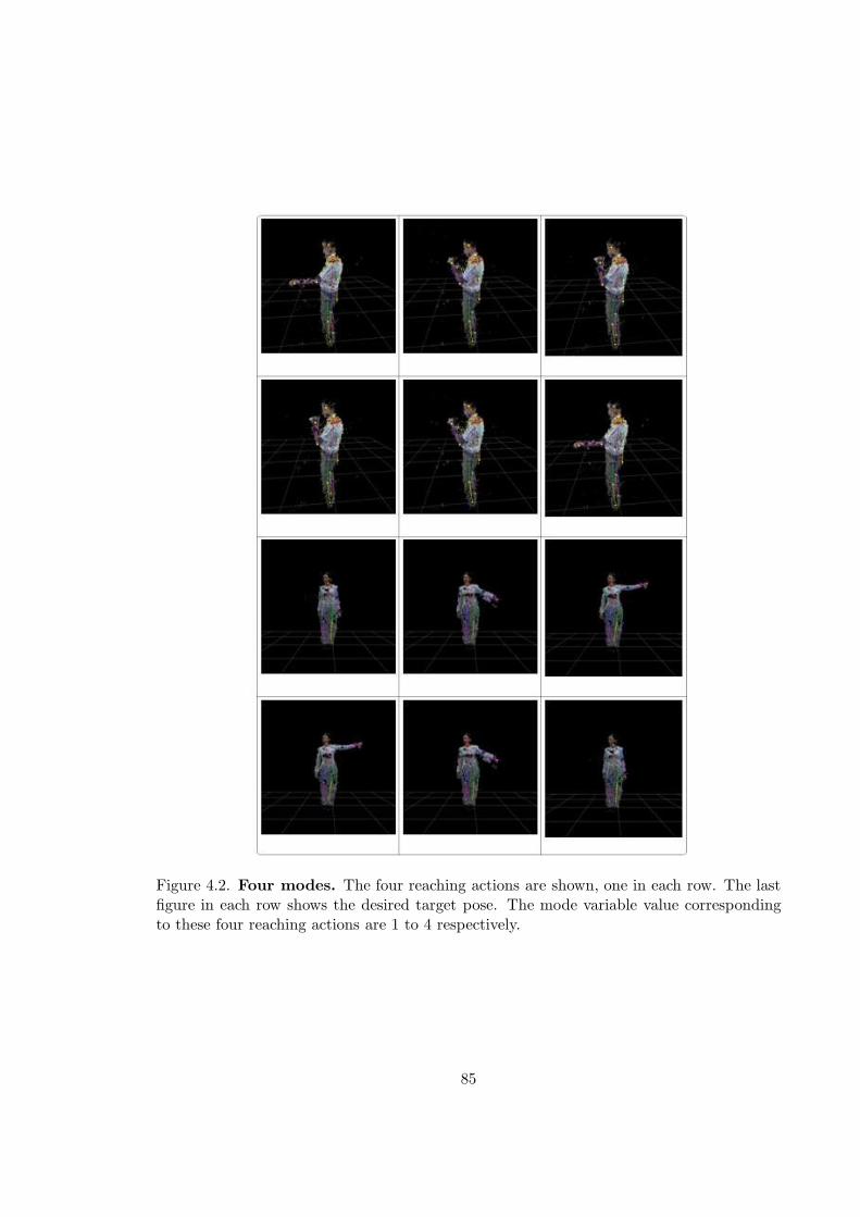
Figure 4.2. Four modes. The four reaching actions are shown, one in each row. The lastfigure in each row shows the desired target pose. The mode variable value correspondingto these four reaching actions are 1 to 4 respectively.
85
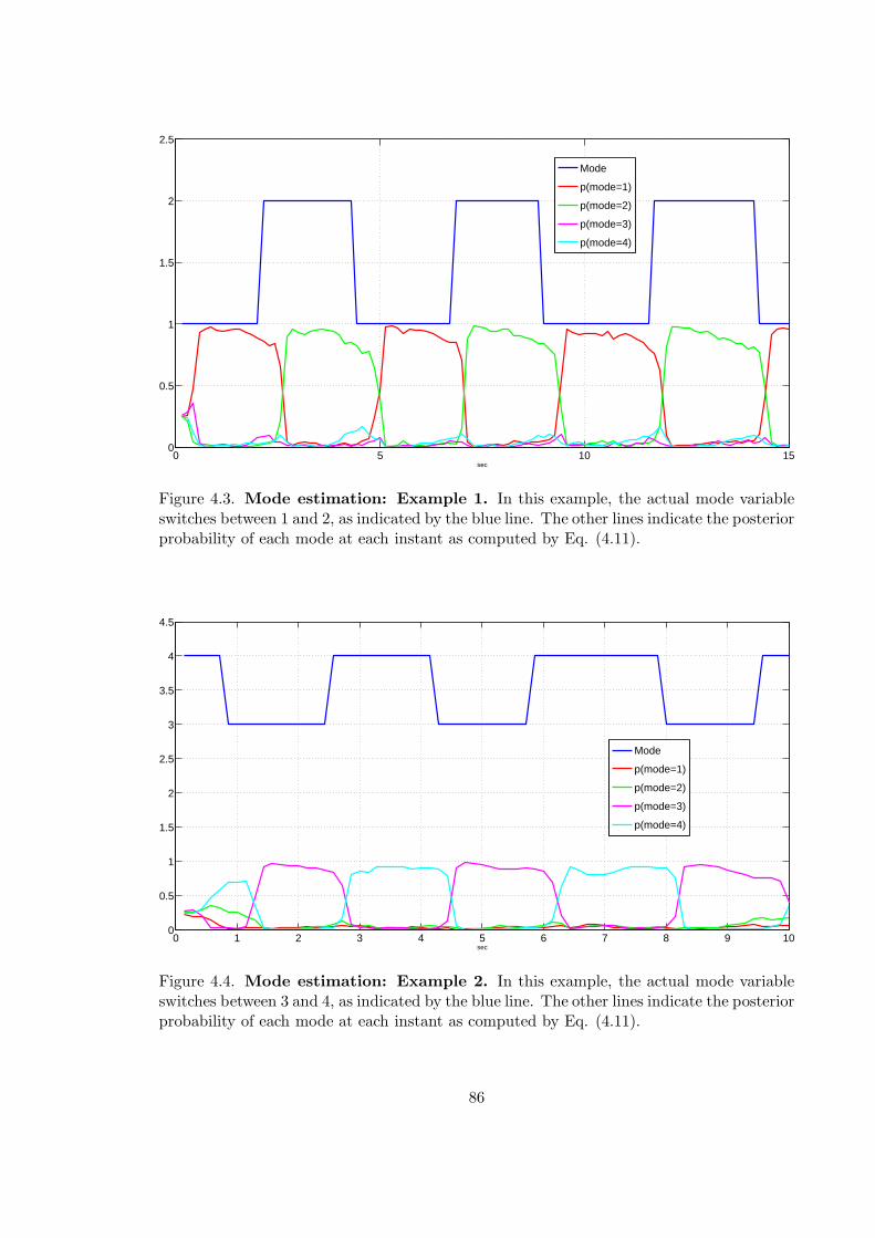
0 5 10 150
0.5
1
1.5
2
2.5
sec
Mode
p(mode=1)
p(mode=2)
p(mode=3)
p(mode=4)
Figure 4.3. Mode estimation: Example 1. In this example, the actual mode variableswitches between 1 and 2, as indicated by the blue line. The other lines indicate the posteriorprobability of each mode at each instant as computed by Eq. (4.11).
0 1 2 3 4 5 6 7 8 9 100
0.5
1
1.5
2
2.5
3
3.5
4
4.5
sec
Mode
p(mode=1)
p(mode=2)
p(mode=3)
p(mode=4)
Figure 4.4. Mode estimation: Example 2. In this example, the actual mode variableswitches between 3 and 4, as indicated by the blue line. The other lines indicate the posteriorprobability of each mode at each instant as computed by Eq. (4.11).
86
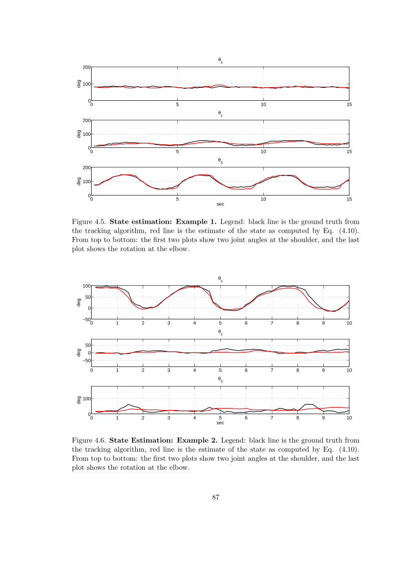
0 5 10 150
100
200
θx
deg
0 5 10 150
100
200
θz
deg
0 5 10 150
100
200
θ3
sec
deg
Figure 4.5. State estimation: Example 1. Legend: black line is the ground truth fromthe tracking algorithm, red line is the estimate of the state as computed by Eq. (4.10).From top to bottom: the first two plots show two joint angles at the shoulder, and the lastplot shows the rotation at the elbow.
0 1 2 3 4 5 6 7 8 9 10−50
0
50
100
θx
deg
0 1 2 3 4 5 6 7 8 9 10
−50
0
50
θz
deg
0 1 2 3 4 5 6 7 8 9 100
100
θ3
sec
deg
Figure 4.6. State Estimation: Example 2. Legend: black line is the ground truth fromthe tracking algorithm, red line is the estimate of the state as computed by Eq. (4.10).From top to bottom: the first two plots show two joint angles at the shoulder, and the lastplot shows the rotation at the elbow.
87
Chapter 5
Conclusion
In this thesis we have shown how an optimal control based representation of human
actions could be used to understand differences in the manner in which people move, and
recognize actions from a library of learnt cost function primitives.
As our simulations in Chapter 2 show, a range of movements can be elegantly captured
by a single cost function structure by varying the cost function weighting parameters. The
optimal control model can automatically generate complex strategies such as countermove-
ments, which are observed in human motion. The effect of body dynamics and variations
in weighting parameters can be studied by simulation.
In the case of the arm movements we studied, we found that the optimal control tra-
jectory changed very slowly in certain parameter ranges, and very rapidly in others. We,
therefore, clustered the optimal trajectories and compared parameter values in terms of
whether they lie in the same cluster or not. We also found that the inertial parameters,
body height and mass, had negligible effect on the optimal arm trajectory.
It is both easy and intuitive to construct a cost function structure for an action since they
represent high-level goals of the action. There is also a vast body of neuroscience literature
proposing and testing different cost function structures for different actions. However, it is
not easy to determine how the different terms of a cost function should be traded off, since
in practice, people do not have a set preference.
88
We proposed a method (Chapter 3) for estimating the weighting parameters of a cost
function from a segmented and labeled data set for an action. We assumed that the structure
of the cost function is known and estimated the unknown weighting parameters by solving
a least squares optimization problem. For simulated data, we found that the parameter
estimates lay in the same cluster as the actual parameter values.
We also tested our method on motion capture data of different subjects performing
reaching and punching actions. We found that subjects did not have a set preference
structure: the parameter estimates for a single subject could show significant variation from
one trial to the next. However, overall, the parameter estimates lay in only in a limited range
of parameter values indicating commonalities in the manner in which subjects interpreted
the task. For instance, in the reaching experiments, the subjects tended to place greater
weight on minimizing the position error than bringing the hand to rest at the target.
We believe this method of constructing cost function primitives and then using them
for estimation can find application in the construction of interactive interfaces, gaming and
imitation learning for robots. Our approach is particularly suited for applications where it
is important to identify, quantify and differentiate the manner in which a particular action
is performed. For instance, our approach could be used to understand how the context in
which an action is performed influences the manner in which it is performed. We suggest
here certain future directions of research related to the work presented in this thesis.
• In estimating cost function parameters from data, we have assumed a purely de-
terministic model. An interesting extension would be to consider models with
noisy control since signal-dependent noise in neural control signals has been found
to play an important role in movement planning ([Harris and Wolpert, 1998] and
[Todorov and Jordan, 2002]).
• We have assumed in our work that the structure of the cost function is known to us.
In actions such as gestures the structure might not be obvious and methods such as
via-point extraction [Wada and Kawato, 2004] could be investigated for extraction of
task constraints.
89

• The model could be extended to include perception processes. In our analysis we
assume that the information required for task definition is noise-free and reliably
available. For instance, in a reaching task the target location is assumed to be known
without any uncertainty. In an actual sensorimotor system, the target location is
procured through visual perception which interacts with the motor system to pro-
vide the required input and if necessary, undertake exploratory measures to procure
information.
The confluence of ideas in neuroscience, robotics and machine learning, combined with
the vast sources of data provided by cameras and sensors, can open up new ways of thinking
about analysis of human actions, that are cognizant of the underlying processes that we use
in producing actions.
90
Bibliography
[Abbeel and Ng, 2004] Abbeel, P. and Ng, A. Y. (2004). Apprenticeship learning via in-verse reinforcement learning. Proceedings of the Twenty-first International Conferenceon Machine Learning.
[Abend et al., 1982] Abend, W., Bizzi, E., and Morasso, P. (1982). Human arm trajectoryformation. Brain, 105(2):331–348.
[Ackerson and Fu, 1970] Ackerson, G. and Fu, K. (1970). On state estimation in switchingenvironments. IEEE Transactions on Automatic Control, 15(1):10–17.
[Alexander, 1997] Alexander, R. M. N. (1997). A minimum energy cost hypothesis forhuman arm trajectories. Biological Cybernetics, 76(2):97–105.
[Anderson and Pandy, 1999] Anderson, F. C. and Pandy, M. G. (1999). A dynamic opti-mization solution for vertical jumping in three dimensions. Comput. Methods Biomech.Biomed. Engin., 2(3):201–231.
[Anderson and Pandy, 2001] Anderson, F. C. and Pandy, M. G. (2001). Dynamic optimiza-tion of human walking. Journal of Biomechanical Engineering, 123:381.
[Andersson, 1985] Andersson, P. (1985). Adaptive forgetting in recursive identificationthrough multiple models. International Journal of Control, 42(5):1175–1194.
[Arulampalam et al., 2002] Arulampalam, S., Maskell, S., Gordon, N., and Clapp, T.(2002). A tutorial on particle filters for on-line non-linear/non-gaussian bayesian tracking.IEEE Transactions on Signal Processing, 50(2):174–188.
[Bernstein, 1967] Bernstein, N. I. (1967). The Coordination and Regulation of Movements.Pergamon, Oxford.
[Berthier et al., 2005] Berthier, N. E., Rosenstein, M. T., and Barto, A. G. (2005). Approxi-mate optimal control as a model for motor learning. Psychological review, 112(2):329–345.
[Betts, 2001] Betts, J. T. (2001). Practical Methods for Optimal Control Using NonlinearProgramming. Society for Industrial Mathematics, SIAM Book Series, Philadelphia.
[Bissacco et al., 2001] Bissacco, A., Chiuso, A., Ma, Y., and Soatto, S. (2001). Recognitionof human gaits. In IEEE Computer Society Conference on Computer Vision and PatternRecognition, 2001., volume 2.
91
[Bizzi et al., 1991] Bizzi, E., Mussa-Ivaldi, F. A., and Giszter, S. (1991). Computationsunderlying the execution of movement: a biological perspective. Science, 253(5017):287–291.
[Blom and Bar-Shalom, 1988] Blom, H. A. P. and Bar-Shalom, Y. (1988). The interact-ing multiple model algorithm for systems with markovian switching coefficients. IEEETransactions on Automatic Control, 33(8):780–783.
[Bobick and Davis, 1996] Bobick, A. and Davis, J. (1996). Real-time recognition of activityusing temporal templates. In 3rd IEEE Workshop on Applications of Computer Vision,1996., pages 39–42.
[Bobick and Davis, 2001] Bobick, A. F. and Davis, J. W. (2001). The recognition of hu-man movement using temporal templates. IEEE Transactions on Pattern Analysis andMachine Intelligence, 23(3):257–267.
[Boers and Driessen, 2003] Boers, Y. and Driessen, J. N. (2003). Interacting multiple modelparticle filter. IEE Proceedings on Radar, Sonar and Navigation, 150(5):344–349.
[Boyd et al., 1982] Boyd, S., Balakrishnan, V., Feron, E., and El Ghaoui, L. (1982). Con-trol system analysis and synthesis via linear matrix inequalities. Control Conference,American, 30.
[Brand and Kettnaker, 2000] Brand, M. and Kettnaker, V. (2000). Discovery and seg-mentation of activities in video. IEEE Transactions on Pattern Analysis and MachineIntelligence, 22(8):844–851.
[Brand et al., 1997] Brand, M., Oliver, N., and Pentland, A. (1997). Coupled hiddenmarkov models for complex action recognition. In IEEE Computer Society Conferenceon Computer Vision and Pattern Recognition (CVPR), pages 994–999.
[Breakwell, 1959] Breakwell, J. V. (1959). The optimization of trajectories. Journal of theSociety for Industrial and Applied Mathematics, pages 215–247.
[Bregler, 1997] Bregler, C. (1997). Learning and recognizing human dynamics in videosequences. Proceedings of IEEE Computer Society Conference on Computer Vision andPattern Recognition (CVPR), 1997., pages 568–574.
[Bruckner et al., 1973] Bruckner, J. M. H., Scott, R. W., and Rea, F. G. (1973). Analysisof multimodal systems. IEEE Transactions on Aerospace and Electronic Systems, pages883–888.
[Bryson and Ho, 1975] Bryson, A. E. and Ho, Y. C. (1975). Applied optimal control :Optimization, Estimation and Control. Taylor and Francis, Bristol, PA.
[Bryson and Ross, 1958] Bryson, A. E. and Ross, S. E. (1958). Optimum rocket trajectorieswith aerodynamic drag. Jet Propulsion, 28(7):465–469.
[Calinon et al., 2007] Calinon, S., Guenter, F., and Billard, A. (2007). On learning, repre-senting, and generalizing a task in a humanoid robot. IEEE Transactions on Systems,Man and Cybernetics Part B, 37(2):286.
92
[Calinon et al., 2005] Calinon, S., Gunter, F., and Billard, A. (2005). Goal-directed imita-tion in a humanoid robot. In IEEE International Conference on Robotics and Automation,volume 1, page 299.
[Canon et al., 1970] Canon, M. D., Cullum, C. D., and Polak, E. (1970). Theory of optimalcontrol and mathematical programming. McGraw-Hill, New York.
[Carlsson and Sullivan, 2001] Carlsson, S. and Sullivan, J. (2001). Action recognition byshape matching to key frames. In Int. Workshop on Models versus Exemplars in ComputerVision, volume 2.
[Cedras and Shah, 1995] Cedras, C. and Shah, M. (1995). Motion-based recognition a sur-vey. Image and Vision Computing, 13(2):129–155.
[Crawford, 1998] Crawford, L. S. (1998). Learning control of complex skills. PhD thesis,University of Califonia, Berkeley.
[de Freitas, 2002] de Freitas, N. (2002). Rao-blackwellised particle filtering for fault diag-nosis. IEEE Aerospace Conference Proceedings, 2002., 4.
[Del Vecchio et al., 2003] Del Vecchio, D., Murray, R. M., and Perona, P. (2003). Decom-position of human motion into dynamics-based primitives with application to drawingtasks. Automatica, 39(12):2085–2098.
[Drumwright et al., 2004] Drumwright, E., Jenkins, O. C., and Mataric, M. J. (2004).Exemplar-based primitives for humanoid movement classification and control. Proceed-ings. IEEE International Conference on Robotics and Automation, 2004., 1.
[Fagg et al., 2002] Fagg, A. H., Shah, A., and Barto, A. G. (2002). A computational modelof muscle recruitment for wrist movements. Journal of Neurophysiology, 88(6):3348–3358.
[Flash and Hogan, 1985] Flash, T. and Hogan, N. (1985). The coordination of arm move-ments: an experimentally confirmed mathematical model. Journal of Neuroscience,5(7):1688–1703.
[Flash and Sejnowski, 2001] Flash, T. and Sejnowski, T. J. (2001). Computational ap-proaches to motor control. Current Opinion in Neurobiology, 11(6):655–662.
[Fod et al., 2002] Fod, A., Mataric, M. J., and Jenkins, O. C. (2002). Automated derivationof primitives for movement classification. Autonomous Robots, 12(1):39–54.
[Fogassi et al., 2005] Fogassi, L., Ferrari, P. F., Gesierich, B., Rozzi, S., Chersi, F., andRizzolatti, G. (2005). Parietal lobe: From action organization to intention understanding.Science, 308(5722):662–667.
[Gavrila, 1999] Gavrila, D. M. (1999). The visual analysis of human movement: A survey.Computer Vision and Image Understanding, 73(1):82–98.
[Guenter et al., 2007] Guenter, F., Hersch, M., Calinon, S., and Billard, A. (2007). Re-inforcement learning for imitating constrained reaching movements. Advanced Robotics,21(13):1521–1544.
[Harris and Wolpert, 1998] Harris, C. M. and Wolpert, D. M. (1998). Signal-dependentnoise determines motor planning. Nature, 394(6695):780–4.
93
[Hogan, 1984] Hogan, N. (1984). An organizing principle for a class of voluntary movements.Journal of Neuroscience, 4(11):2745–2754.
[Intille and Bobick, 1998] Intille, S. S. and Bobick, A. F. (1998). Representation and vi-sual recognition of complex, multi-agent actions using belief networks. In Workshop onInterpretation of Visual Motion (CVPR).
[Jacobson and Mayne, 1970] Jacobson, D. H. and Mayne, D. Q. (1970). Differential dy-namic programming. Modern Analytic and Computational Methods in Science and Math-ematics, 24.
[Jenkins and Mataric, 2003] Jenkins, O. C. and Mataric, M. J. (2003). Automated deriva-tion of behavior vocabularies for autonomous humanoid motion. In Second internationaljoint conference on Autonomous agents and multiagent systems, pages 225–232. ACMNew York, NY, USA.
[Jenkins et al., 2007] Jenkins, O. C., Serrano, G. G., and Loper, M. M. (2007). Interactivehuman pose and action recognition using dynamical motion primitives. InternationalJournal of Humanoid Robotics, 4(2):365–386.
[Kalman, 1979] Kalman, R. E. (1979). When is a linear control system optimal? Frequency-Response Methods in Control Systems, page 71.
[Karlsson and Bergman, 2000] Karlsson, R. and Bergman, N. (2000). Auxiliary particlefilters for tracking a maneuvering target. Proceedings of the 39th IEEE Conference onDecision and Control, 2000, 4.
[Kelley, 1960] Kelley, H. J. (1960). Gradient theory of optimal flight paths. J. AmericanRocket Soc., 30.
[Kelley et al., 1963] Kelley, H. J., Kopp, R. E., and Moyer, H. G. (1963). A trajectoryoptimization technique based upon the theory of the second variation. In AIAA Astro-dynamics Conference, New Haven, CT.
[Kellokumpu et al., 2005] Kellokumpu, V., Pietikinen, M., and Heikkil, J. (2005). Humanactivity recognition using sequences of postures. In IAPR Conference on Machine VisionApplications, pages 570–573, Tsukuba Science City, Japan.
[Kirk, 2004] Kirk, D. E. (2004). Optimal Control Theory: An Introduction. Courier DoverPublications, Mineola, NY.
[Kojima et al., 2002] Kojima, A., Tamura, T., and Fukunaga, K. (2002). Natural languagedescription of human activities from video images based on concept hierarchy of actions.International Journal of Computer Vision, 50(2):171–184.
[Kuo, 1995] Kuo, A. D. (1995). An optimal control model for analyzing human posturalbalance. IEEE Transactions on Biomedical Engineering, 42(1):87–101.
[Larin, 2003] Larin, V. B. (2003). About the inverse problem of optimal control. Appl.Comput. Math, 2(2):90–97.
[Lasdon et al., 1967] Lasdon, L., Mitter, S., and Waren, A. (1967). The conjugate gra-dient method for optimal control problems. IEEE Transactions on Automatic Control,12(2):132–138.
94
[Li and Todorov, 2004] Li, W. and Todorov, E. (2004). Iterative linear-quadratic regulatordesign for nonlinear biological movement systems. Proceedings of the First InternationalConference on Informatics in Control, Automation, and Robotics, pages 222–229.
[Lien et al., 2007] Lien, J. M., Kurillo, G., and Bajcsy, R. (2007). Skeleton-based datacompression for multi-camera tele-immersion system. Proceedings of International Sym-posium on Visual Computing (ISVC 2007), Lake Tahoe, CA, pages 26–28.
[M. A. McDowell, 2008] M. A. McDowell, C.D. Fryar, C. L. O. K. M. F. (2008). Anthro-pometric reference data for children and adults : United states, 2003-2006. Technicalreport, Centers for Disease Control and Prevention.
[Mazor et al., 1998] Mazor, E., Averbuch, A., Bar-Shalom, Y., and Dayan, J. (1998). In-teracting multiple model methods in target tracking: a survey. IEEE Transactions onAerospace and Electronic Systems, 34(1):103–123.
[McGinnity and Irwin, 2000] McGinnity, S. and Irwin, G. W. (2000). Multiple model boot-strap filter for maneuvering target tracking. IEEE Transactions on Aerospace and Elec-tronic Systems, 36(3):1006–1012.
[Miyamoto et al., 2004] Miyamoto, H., Nakano, E., Wolpert, D. M., and Kawato, M.(2004). Tops (task optimization in the presence of signal-dependent noise) model. Systemsand Computers in Japan, 35(11):48–58.
[Morasso, 1981] Morasso, P. (1981). Spatial control of arm movements. Experimental BrainResearch, 42(2):223–227.
[Moylan and Anderson, 1973] Moylan, P. and Anderson, B. (1973). Nonlinear regulatortheory and an inverse optimal control problem. IEEE Transactions on Automatic Control,18(5):460–465.
[Murray et al., 1994] Murray, R. M., Li, Z., and Sastry, S. S. (1994). A MathematicalIntroduction to Robotic Manipulation. CRC Press, Boca Rotan, FL.
[Mussa-Ivaldi and Bizzi, 2000] Mussa-Ivaldi, F. A. and Bizzi, E. (2000). Motor learningthrough the combination of primitives. Philosophical Transactions of the Royal SocietyB: Biological Sciences, 355(1404):1755.
[Nakano et al., 1999] Nakano, E., Imamizu, H., Osu, R., Uno, Y., Gomi, H., Yoshioka, T.,and Kawato, M. (1999). Quantitative examinations of internal representations for armtrajectory planning: Minimum commanded torque change model. Journal of Neurophys-iology, 81(5):2140–2155.
[Ng and Russell, 2000] Ng, A. Y. and Russell, S. (2000). Algorithms for inverse reinforce-ment learning. Proceedings of the Seventeenth International Conference on MachineLearning, pages 663–670.
[Nishii and Murakami, 2002] Nishii, J. and Murakami, T. (2002). Energetic optimality ofarm trajectory. In Int. Conf. on Biomechanics of Man, page 3033.
[Nori and Frezza, 2005] Nori, F. and Frezza, R. (2005). A control theory approach to theanalysis and synthesis of the experimentally observed motion primitives. Biological Cy-bernetics, 93(5):323–342.
95
[Ogale et al., 2005] Ogale, A. S., Karapurkar, A., and Aloimonos, Y. (2005). View-invariantmodeling and recognition of human actions using grammars. In Workshop on DynamicalVision at ICCV, volume 5. Springer.
[Oliver et al., 2004] Oliver, N., Garg, A., and Horvitz, E. (2004). Layered representationsfor learning and inferring office activity from multiple sensory channels. Computer Visionand Image Understanding, 96(2):163–180.
[Pandy et al., 1995] Pandy, M. G., Garner, B. A., and Anderson, F. C. (1995). Optimalcontrol of non-ballistic muscular movements: a constraint-based performance criterionfor rising from a chair. J Biomech Eng, 117(1):15–26.
[Park and Aggarwal, 2004] Park, S. and Aggarwal, J. K. (2004). A hierarchical bayesiannetwork for event recognition of human actions and interactions. Multimedia Systems,10(2):164–179.
[Pitt and Shephard, 1999] Pitt, M. K. and Shephard, N. (1999). Filtering via simulation:Auxiliary particle filters. Journal of the American Statistical Association, 94(446):590–599.
[Pitt and Shephard, 2001] Pitt, M. K. and Shephard, N. (2001). Auxiliary variable basedparticle filters. In Doucet, A., editor, Sequential Monte Carlo Methods in Practice.Springer-Verlag, New York.
[Polak, 1973] Polak, E. (1973). An historical survey of computational methods in optimalcontrol. SIAM Review, 15(2):553–584.
[Polana and Nelson, 1997] Polana, R. and Nelson, R. C. (1997). Detection and recognitionof periodic, nonrigid motion. International Journal of Computer Vision, 23(3):261–282.
[Ramachandran and Amir, 2007] Ramachandran, D. and Amir, E. (2007). Bayesian inversereinforcement learning. International Joint Conference on Artificial Intelligence, 51:2586–2591.
[Rekasius and Hsia, 1964] Rekasius, Z. and Hsia, T. (1964). On an inverse problem inoptimal control. IEEE Transactions on Automatic Control, 9(4):370–375.
[Rizzolatti and Craighero, 2004] Rizzolatti, G. and Craighero, L. (2004). The mirror-neuron system. Annual Review of Neuroscience, 27(1):169–192.
[Rui and Anandan, 2000] Rui, Y. and Anandan, P. (2000). Segmenting visual actions basedon spatio-temporal motion patterns. In IEEE Conference on Computer Vision and Pat-tern Recognition, 2000., volume 1.
[Safonova et al., 2004] Safonova, A., Hodgins, J. K., and Pollard, N. S. (2004). Synthesizingphysically realistic human motion in low-dimensional, behavior-specific spaces. ACMTransactions on Graphics (TOG), 23(3):514–521.
[Sargent and Pollard, 1970] Sargent, R. and Pollard, G. P. (1970). Off line computation ofoptimal controls for a plate distillation column. Automatica, 6:59–76.
[Sargent, 2000] Sargent, R. W. H. (2000). Optimal control. Journal of Computational andApplied Mathematics, 124(1-2):361–371.
96
[Schaal et al., 2003] Schaal, S., Ijspeert, A., and Billard, A. (2003). Computational ap-proaches to motor learning by imitation. Philosophical Transactions of the Royal SocietyB: Biological Sciences, 358(1431):537.
[Schaal et al., 2004] Schaal, S., Peters, J., Nakanishi, J., and Ijspeert, A. (2004). Learningmovement primitives. International Symposium on Robotics Research (ISRR2003).
[Scott, 2004] Scott, S. H. (2004). Optimal feedback control and the neural basis of volitionalmotor control. Nature Reviews Neuroscience, 5(7):532–546.
[Sminchisescu et al., 2006] Sminchisescu, C., Kanaujia, A., and Metaxas, D. (2006). Con-ditional models for contextual human motion recognition. Computer Vision and ImageUnderstanding, 104(2-3):210–220.
[Soechting et al., 1995] Soechting, J. F., Buneo, C. A., Herrmann, U., and Flanders, M.(1995). Moving effortlessly in three dimensions: does donders’ law apply to arm move-ment? Journal of Neuroscience, 15(9):6271–6280.
[Stengel, 1994] Stengel, R. F. (1994). Optimal control and estimation. Courier Dover Pub-lications, New York.
[Stoer and Bulirsch, 2002] Stoer, J. and Bulirsch, R. (2002). Introduction to numericalanalysis. Springer, New York.
[Taniai and Nishii, 2008] Taniai, Y. and Nishii, J. (2008). Optimality of reaching move-ments based on energetic cost under the influence of signal-dependent noise. LectureNotes in Computer Science, 4984:1091–1099.
[Todorov, 2001] Todorov, E. (2001). Arm movements minimize a combination of error andeffort. Neural Control of Movement, 11.
[Todorov, 2002] Todorov, E. (2002). Cosine tuning minimizes motor errors. Neural Com-putation, 14(6):1233–1260.
[Todorov, 2004] Todorov, E. (2004). Optimality principles in sensorimotor control (review).Nature Neuroscience, 7(9):907.
[Todorov and Jordan, 2002] Todorov, E. and Jordan, M. I. (2002). Optimal feedback con-trol as a theory of motor coordination. Nature Neuroscience, 5(11):1226–1235.
[Todorov et al., 2005] Todorov, E., Li, W., and Pan, X. (2005). From task parameters tomotor synergies: a hierarchical framework for approximately optimal control of redundantmanipulators. Journal of Robotic Systems, 22(11):691–710.
[Tsang et al., 1975] Tsang, T. H., Himmelblau, D. M., and Edgar, T. F. (1975). Optimalcontrol via collocation and non-linear programming. Int. J. Control, 21(5):763–768.
[Uno et al., 1989] Uno, Y., Kawato, M., and Suzuki, R. (1989). Formation and control ofoptimal trajectory in human multijoint arm movement. Biological Cybernetics, 61(2):89–101.
[van Beers et al., 2004] van Beers, R. J., Haggard, P., and Wolpert, D. M. (2004). The roleof execution noise in movement variability. Journal of Neurophysiology, 91(2):1050–1063.
97
[Wada and Kawato, 2004] Wada, Y. and Kawato, M. (2004). A via-point time optimizationalgorithm for complex sequential trajectory formation. Neural Networks, 17(3):353–364.
[Wang et al., 2003] Wang, L., Hu, W., and Tan, T. (2003). Recent developments in humanmotion analysis. Pattern recognition, 36(3):585–601.
[Wang and Suter, 2007] Wang, L. and Suter, D. (2007). Learning and matching of dynamicshape manifolds for human action recognition. IEEE Transactions on Image Processing,16(6):1646–1661.
[Weinland et al., 2007] Weinland, D., Boyer, E., and Ronfard, R. (2007). Action recognitionfrom arbitrary views using 3d exemplars. In Int. Conference on Computer Vision (ICCV),volume 5, page 8.
[Weinland et al., 2006] Weinland, D., Ronfard, R., and Boyer, E. (2006). Automatic dis-covery of action taxonomies from multiple views. In Proceedings of the IEEE Conferenceon Computer Vision and Pattern Recognition.
[Winter, 1990] Winter, D. A. (1990). Biomechanics and motor control of human movement.Wiley-Interscience, New York.
[Wolpert and Ghahramani, 2000] Wolpert, D. M. and Ghahramani, Z. (2000). Computa-tional principles of movement neuroscience. Nat Neurosci, 3:1212–1217.
[Wolpert et al., 1995] Wolpert, D. M., Ghahramani, Z., and Jordan, M. I. (1995). Arearm trajectories planned in kinematic or dynamic coordinates? an adaptation study.Experimental Brain Research, 103(3):460–470.
[Yamato et al., 1992] Yamato, J., Ohya, J., and Ishii, K. (1992). Recognizing human ac-tion in time-sequential images using hidden markov model. In IEEE Computer SocietyConference on Computer Vision and Pattern Recognition (CVPR), pages 379–385.
98
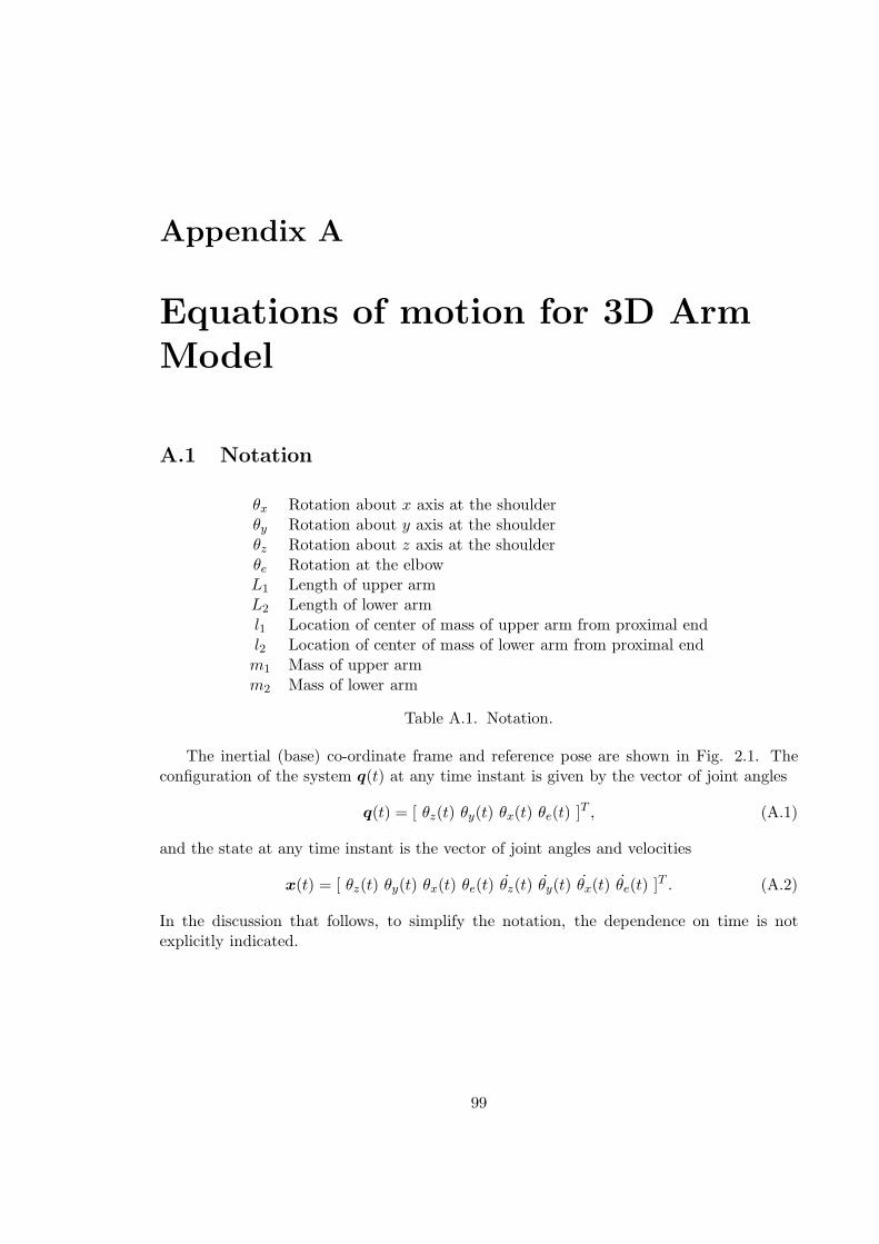
Appendix A
Equations of motion for 3D Arm
Model
A.1 Notation
θx Rotation about x axis at the shoulderθy Rotation about y axis at the shoulderθz Rotation about z axis at the shoulderθe Rotation at the elbowL1 Length of upper armL2 Length of lower arml1 Location of center of mass of upper arm from proximal endl2 Location of center of mass of lower arm from proximal endm1 Mass of upper armm2 Mass of lower arm
Table A.1. Notation.
The inertial (base) co-ordinate frame and reference pose are shown in Fig. 2.1. Theconfiguration of the system q(t) at any time instant is given by the vector of joint angles
q(t) = [ θz(t) θy(t) θx(t) θe(t) ]T , (A.1)
and the state at any time instant is the vector of joint angles and velocities
x(t) = [ θz(t) θy(t) θx(t) θe(t) θz(t) θy(t) θx(t) θe(t) ]T . (A.2)
In the discussion that follows, to simplify the notation, the dependence on time is notexplicitly indicated.
99
A.2 Forward Kinematics
The twists corresponding to the four degrees of freedom of this model are
ξx = [ 0 0 0 1 0 0 ]T
ξy = [ 0 0 0 0 1 0 ]T
ξz = [ 0 0 0 0 0 1 ]T
ξe = [ − L1 0 0 0 0 1 ]T (A.3)
The forward kinematic map that computes the location of the end-effector (hand) from thejoint angle configuration of the arm can be found using the product of exponentials formula(see Chapter 2 of [Murray et al., 1994] for details). The location of the hand, e ∈ ℜ3 isgiven by
e = eξzθzeξyθyeξxθxeξeθe [ 0 − (L1 + L2) 0 1]T (A.4)
where eξzθz is the exponential of the twist ξz and can be computed in closed form from thedefinition of the twist and the value of joint angle (see page 42 [Murray et al., 1994] for theformula). Thus the function e(·) ∈ ℜ3 in Eq. 2.7 is given by
e =
L1(−cθz sθx sθy + cθx sθz ) + L2(cθy cθz sθe + cθe (−cθz sθx sθy + cθx sθz ))−L1(cθx cθz + sθx sθy sθz ) − L2(−cθy sθe sθz + cθe (cθx cθz + sθx sθy sθz ))
−L1cθy sθx − L2(cθe cθy sθx + sθe sθy )
,
(A.5)where cθz and sθz denote the cosine and sine of the indicated joint angle.
A.3 Dynamics
There are two links in our model - the upper arm is the first link and the lower arm isthe second link. A co-ordinate frame is attached to the center of mass of each link. Thebody Jacobian of the first link, J1, is given by
l1cθx cθy −l1sθx 0 00 0 0 0
l1sθy 0 −l1 0−sθy 0 1 0
cθy sθx cθx 0 0cθy cθx −sθx 0 0
. (A.6)
The body Jacobian of the second link, J2, is given by
(l2 + L1cθe)cθx cθy −(l2 + L1cθe)sθx 0 l2−L1cθx cθy sθe L1sθe sθx 0 0
l2(−cθy sθe sθx + cθe sθy) + L1sθy −l2cθx sθe −l2cθe − L1 0cθy sθe sθx − cθe sθy cθx sθe cθe 0cθe cθy sθx + sθe sθy cθe cθx −sθe 0
cθx cθy −sθx 0 1
. (A.7)
The Jacobian matrices can be computed from the definition of the co-ordinate frames andthe structure of the model and can be used to compute the instantaneous velocity of theend-effector (See Chapter 2 of [Murray et al., 1994] for details).
100
The generalized inertia matrix of the i-th link, denoted by Mi is a 6 × 6 matrix of theform [
miI3 03
03 Ii,
]
(A.8)
where Ii denotes the 3 × 3 inertia tensor of the i-th link expressed in the link co-ordinateframe. In our case the inertia tensors for both links are diagonal and of the form
Ii,xx 0 00 Ii,yy 00 0 Ii,zz
. (A.9)
Assuming that the links are uniform cylinders of radius ri, the terms of the inertia tensormatrix for the i-th link are are given by
Ii,zz = Ii,xx =mi
12(L2
i + 3r2i ),
Ii,yy =mir
2i
12.
(A.10)
The manipulator inertia matrix M(·) in Eq. 1.1 can be computed from the link Jacobiansand the generalized inertia matrices:
M(q) = J T1 (q)M1J1(q) + J T
2 (q)M2J2(q). (A.11)
The total kinetic energy of the system is
1
2qT M(q)q. (A.12)
Let hi(q) denote the height of the center of mass of the i-th link. In our model
h1 = −l1cθy sθx,
h2 = −L1cθy sθx − l2(cθe cθy sθx + sθe sθy ). (A.13)
The potential energy of the system is
m1gh1 + m2gh2, (A.14)
where g is the gravitational constant. Combining we have the Lagrangian of the system,
L(q, q) =1
2qT M(q)q − (m1gh1(q) + m2gh2(q)), (A.15)
from which which we can derive the equations of motion of the system. The equations ofmotion of the system are given by Lagrange’s equations (See p. 158 [Murray et al., 1994])
d
dt
∂L
∂q−
∂L
∂q= u, (A.16)
where u is the vector of joint torques. As discussed in Chapter 3 of [Murray et al., 1994],the equations of motion can be re-written in the form
M(q)q + C(q, q)q + N(q) = u, (A.17)
101
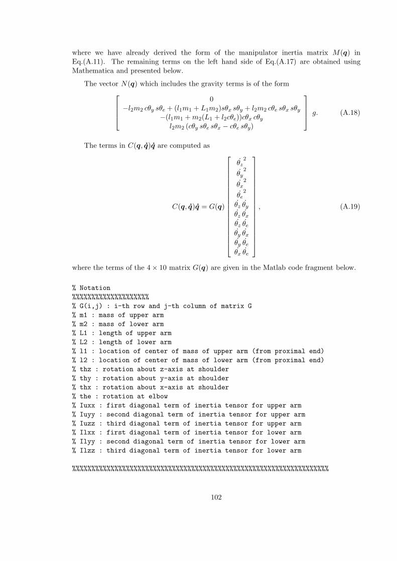
where we have already derived the form of the manipulator inertia matrix M(q) inEq.(A.11). The remaining terms on the left hand side of Eq.(A.17) are obtained usingMathematica and presented below.
The vector N(q) which includes the gravity terms is of the form
0−l2m2 cθy sθe + (l1m1 + L1m2)sθx sθy + l2m2 cθe sθx sθy
−(l1m1 + m2(L1 + l2cθe))cθx cθy
l2m2 (cθy sθe sθx − cθe sθy)
g. (A.18)
The terms in C(q, q)q are computed as
C(q, q)q = G(q)
θz2
θy2
θx2
θe2
θz θy
θz θx
θz θe
θy θx
θy θe
θx θe
, (A.19)
where the terms of the 4 × 10 matrix G(q) are given in the Matlab code fragment below.
% Notation
%%%%%%%%%%%%%%%%%%%%
% G(i,j) : i-th row and j-th column of matrix G
% m1 : mass of upper arm
% m2 : mass of lower arm
% L1 : length of upper arm
% L2 : length of lower arm
% l1 : location of center of mass of upper arm (from proximal end)
% l2 : location of center of mass of lower arm (from proximal end)
% thz : rotation about z-axis at shoulder
% thy : rotation about y-axis at shoulder
% thx : rotation about x-axis at shoulder
% the : rotation at elbow
% Iuxx : first diagonal term of inertia tensor for upper arm
% Iuyy : second diagonal term of inertia tensor for upper arm
% Iuzz : third diagonal term of inertia tensor for upper arm
% Ilxx : first diagonal term of inertia tensor for lower arm
% Ilyy : second diagonal term of inertia tensor for lower arm
% Ilzz : third diagonal term of inertia tensor for lower arm
%%%%%%%%%%%%%%%%%%%%%%%%%%%%%%%%%%%%%%%%%%%%%%%%%%%%%%%%%%%%%%%%%%%
102
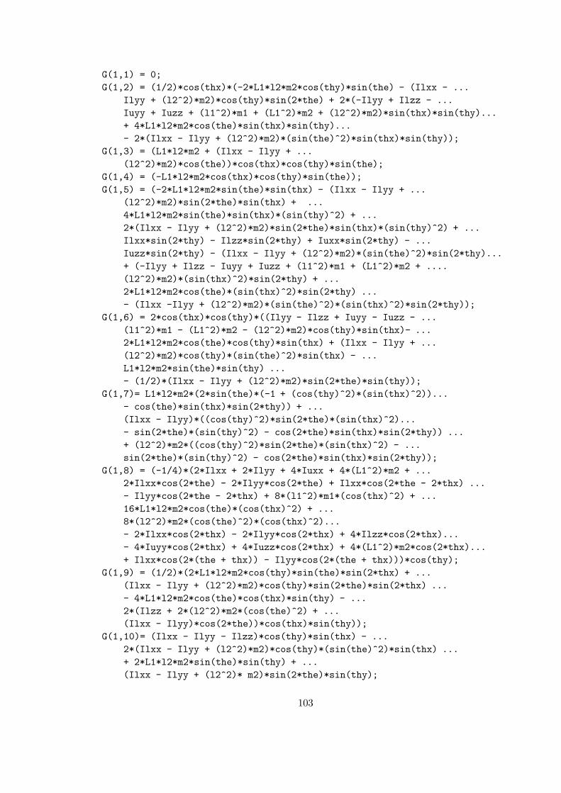
G(1,1) = 0;
G(1,2) = (1/2)*cos(thx)*(-2*L1*l2*m2*cos(thy)*sin(the) - (Ilxx - ...
Ilyy + (l2^2)*m2)*cos(thy)*sin(2*the) + 2*(-Ilyy + Ilzz - ...
Iuyy + Iuzz + (l1^2)*m1 + (L1^2)*m2 + (l2^2)*m2)*sin(thx)*sin(thy)...
+ 4*L1*l2*m2*cos(the)*sin(thx)*sin(thy)...
- 2*(Ilxx - Ilyy + (l2^2)*m2)*(sin(the)^2)*sin(thx)*sin(thy));
G(1,3) = (L1*l2*m2 + (Ilxx - Ilyy + ...
(l2^2)*m2)*cos(the))*cos(thx)*cos(thy)*sin(the);
G(1,4) = (-L1*l2*m2*cos(thx)*cos(thy)*sin(the));
G(1,5) = (-2*L1*l2*m2*sin(the)*sin(thx) - (Ilxx - Ilyy + ...
(l2^2)*m2)*sin(2*the)*sin(thx) + ...
4*L1*l2*m2*sin(the)*sin(thx)*(sin(thy)^2) + ...
2*(Ilxx - Ilyy + (l2^2)*m2)*sin(2*the)*sin(thx)*(sin(thy)^2) + ...
Ilxx*sin(2*thy) - Ilzz*sin(2*thy) + Iuxx*sin(2*thy) - ...
Iuzz*sin(2*thy) - (Ilxx - Ilyy + (l2^2)*m2)*(sin(the)^2)*sin(2*thy)...
+ (-Ilyy + Ilzz - Iuyy + Iuzz + (l1^2)*m1 + (L1^2)*m2 + ....
(l2^2)*m2)*(sin(thx)^2)*sin(2*thy) + ...
2*L1*l2*m2*cos(the)*(sin(thx)^2)*sin(2*thy) ...
- (Ilxx -Ilyy + (l2^2)*m2)*(sin(the)^2)*(sin(thx)^2)*sin(2*thy));
G(1,6) = 2*cos(thx)*cos(thy)*((Ilyy - Ilzz + Iuyy - Iuzz - ...
(l1^2)*m1 - (L1^2)*m2 - (l2^2)*m2)*cos(thy)*sin(thx)- ...
2*L1*l2*m2*cos(the)*cos(thy)*sin(thx) + (Ilxx - Ilyy + ...
(l2^2)*m2)*cos(thy)*(sin(the)^2)*sin(thx) - ...
L1*l2*m2*sin(the)*sin(thy) ...
- (1/2)*(Ilxx - Ilyy + (l2^2)*m2)*sin(2*the)*sin(thy));
G(1,7)= L1*l2*m2*(2*sin(the)*(-1 + (cos(thy)^2)*(sin(thx)^2))...
- cos(the)*sin(thx)*sin(2*thy)) + ...
(Ilxx - Ilyy)*((cos(thy)^2)*sin(2*the)*(sin(thx)^2)...
- sin(2*the)*(sin(thy)^2) - cos(2*the)*sin(thx)*sin(2*thy)) ...
+ (l2^2)*m2*((cos(thy)^2)*sin(2*the)*(sin(thx)^2) - ...
sin(2*the)*(sin(thy)^2) - cos(2*the)*sin(thx)*sin(2*thy));
G(1,8) = (-1/4)*(2*Ilxx + 2*Ilyy + 4*Iuxx + 4*(L1^2)*m2 + ...
2*Ilxx*cos(2*the) - 2*Ilyy*cos(2*the) + Ilxx*cos(2*the - 2*thx) ...
- Ilyy*cos(2*the - 2*thx) + 8*(l1^2)*m1*(cos(thx)^2) + ...
16*L1*l2*m2*cos(the)*(cos(thx)^2) + ...
8*(l2^2)*m2*(cos(the)^2)*(cos(thx)^2)...
- 2*Ilxx*cos(2*thx) - 2*Ilyy*cos(2*thx) + 4*Ilzz*cos(2*thx)...
- 4*Iuyy*cos(2*thx) + 4*Iuzz*cos(2*thx) + 4*(L1^2)*m2*cos(2*thx)...
+ Ilxx*cos(2*(the + thx)) - Ilyy*cos(2*(the + thx)))*cos(thy);
G(1,9) = (1/2)*(2*L1*l2*m2*cos(thy)*sin(the)*sin(2*thx) + ...
(Ilxx - Ilyy + (l2^2)*m2)*cos(thy)*sin(2*the)*sin(2*thx) ...
- 4*L1*l2*m2*cos(the)*cos(thx)*sin(thy) - ...
2*(Ilzz + 2*(l2^2)*m2*(cos(the)^2) + ...
(Ilxx - Ilyy)*cos(2*the))*cos(thx)*sin(thy));
G(1,10)= (Ilxx - Ilyy - Ilzz)*cos(thy)*sin(thx) - ...
2*(Ilxx - Ilyy + (l2^2)*m2)*cos(thy)*(sin(the)^2)*sin(thx) ...
+ 2*L1*l2*m2*sin(the)*sin(thy) + ...
(Ilxx - Ilyy + (l2^2)* m2)*sin(2*the)*sin(thy);
103

G(2,1) = (1/2)*(2*L1*l2*m2*sin(the)*sin(thx) + ...
(Ilxx - Ilyy + (l2^2)*m2)*sin(2*the)*sin(thx) - ...
4*L1*l2*m2*sin(the)*sin(thx)*(sin(thy)^2)...
-2*(Ilxx - Ilyy + (l2^2)*m2)*sin(2*the)*sin(thx)*(sin(thy)^2) ...
- Ilxx*sin(2*thy) + Ilzz*sin(2*thy) - Iuxx*sin(2*thy) ...
+ Iuzz*sin(2*thy) + (Ilxx - Ilyy + ...
(l2^2)* m2)*(sin(the)^2)*sin(2*thy)...
+ (Ilyy - Ilzz + Iuyy - Iuzz - (l1^2)*m1 - (L1^2)*m2 - ...
(l2^2)*m2)*(sin(thx)^2)*sin(2*thy)...
- 2*L1*l2*m2*cos(the)*(sin(thx)^2)*sin(2*thy) ...
+ (Ilxx - Ilyy + (l2^2)*m2)*(sin(the)^2)*(sin(thx)^2)*sin(2*thy));
G(2,2) = 0;
G(2,3) = (-L1*l2*m2 + (-Ilxx + Ilyy - ...
(l2^2)*m2)*cos(the))*sin(the)*sin(thx);
G(2,4) = L1*l2*m2*sin(the)*sin(thx);
G(2,5) = 0;
G(2,6) = (Ilxx + Ilyy - Ilzz + Iuxx + Iuyy - Iuzz)*cos(thy) ...
+ 2*(-Ilyy + Ilzz - Iuyy + Iuzz + (l1^2)*m1 + ...
(L1^2)*m2 + (l2^2)*m2)*cos(thy)*(sin(thx)^2)...
+ 4*L1*l2*m2*cos(the)*cos(thy)*(sin(thx)^2) - ...
2*(Ilxx - Ilyy + (l2^2)*m2)*cos(thy)*(sin(the)^2)*(sin(thx)^2) + ...
2*L1*l2*m2*sin(the)*sin(thx)*sin(thy) + (Ilxx - Ilyy + ...
(l2^2)*m2)*sin(2*the)*sin(thx)*sin(thy);
G(2,7) = cos(thx)*(2*L1*l2*m2*cos(thy)*sin(the)*sin(thx) + ...
(Ilxx -Ilyy + (l2^2)*m2)*cos(thy)*sin(2*the)*sin(thx) + ...
(Ilzz + (-Ilxx + Ilyy)*cos(2*the) + ...
2*(l2^2)*m2*(sin(the)^2))*sin(thy));
G(2,8) = 2*cos(thx)*(-Ilyy + Ilzz -Iuyy + Iuzz + ...
(l1^2)*m1 + (L1^2)*m2 + 2*L1*l2*m2*cos(the) +...
(l2^2)*m2*(cos(the)^2) + (-Ilxx + Ilyy)*(sin(the)^2))*sin(thx);
G(2,9) = 2*sin(the)*((Ilxx - Ilyy)*cos(the)*(cos(thx)^2) + ...
(l2^2)*m2*cos(the)*(cos(thx)^2) - L1*l2*m2*(sin(thx)^2));
G(2,10) = -cos(thx)*(Ilzz + (-Ilxx + Ilyy)*cos(2*the) +...
2*(l2^2)*m2*(sin(the)^2));
G(3,1) = cos(thx)*cos(thy)*((-Ilyy+ Ilzz - Iuyy + Iuzz + ...
(l1^2)*m1 + (L1^2)*m2 + (l2^2)*m2)*cos(thy)*sin(thx) + ...
2*L1*l2*m2*cos(the)*cos(thy)*sin(thx) + (-Ilxx + Ilyy - ...
(l2^2)*m2)*cos(thy)*(sin(the)^2)*sin(thx) + ...
L1*l2*m2*sin(the)*sin(thy) + (Ilxx - Ilyy + ...
(l2^2)*m2)*cos(the)*sin(the)*sin(thy));
G(3,2) =(-1/4)*(-Ilxx - Ilyy + 2*Ilzz - 2*Iuyy + ...
2*Iuzz + 2*(l1^2)*m1 + 2*(L1^2)*m2 + 4*L1*l2*m2*cos(the)...
+ 2*(l2^2)*m2*(cos(the)^2)...
+ Ilxx*cos(2*the) - Ilyy*cos(2*the))* sin(2*thx);
104
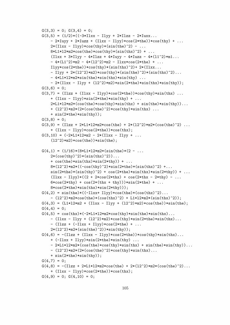
G(3,3) = 0; G(3,4) = 0;
G(3,5) = (1/2)*((-3*Ilxx - Ilyy + 2*Ilzz - 2*Iuxx...
- 2*Iuyy + 2*Iuzz + (Ilxx - Ilyy)*cos(2*the))*cos(thy) + ...
2*(Ilxx - Ilyy)*cos(thy)*(sin(the)^2) - ...
8*L1*l2*m2*cos(the)*cos(thy)*(sin(thx)^2) + ...
(Ilxx + 3*Ilyy - 4*Ilzz + 4*Iuyy - 4*Iuzz - 4*(l1^2)*m1...
- 4*(L1^2)*m2 - 4*(l2^2)*m2 - Ilxx*cos(2*the) + ...
Ilyy*cos(2*the))*cos(thy)*(sin(thx)^2)+ 2*(Ilxx...
- Ilyy + 2*(l2^2)*m2)*cos(thy)*(sin(the)^2)*(sin(thx)^2)...
- 4*L1*l2*m2*sin(the)*sin(thx)*sin(thy) ...
- 2*(Ilxx - Ilyy + (l2^2)*m2)*sin(2*the)*sin(thx)*sin(thy));
G(3,6) = 0;
G(3,7) = (Ilzz + (Ilxx - Ilyy)*cos(2*the))*cos(thy)*sin(thx) ...
+ (Ilxx - Ilyy)*sin(2*the)*sin(thy) + ...
2*L1*l2*m2*(cos(the)*cos(thy)*sin(thx) + sin(the)*sin(thy))...
+ (l2^2)*m2*(2*(cos(the)^2)*cos(thy)*sin(thx) ...
+ sin(2*the)*sin(thy));
G(3,8) = 0;
G(3,9) = (Ilzz + 2*L1*l2*m2*cos(the) + 2*(l2^2)*m2*(cos(the)^2) ...
+ (Ilxx - Ilyy)*cos(2*the))*cos(thx);
G(3,10) = (-2*L1*l2*m2 - 2*(Ilxx - Ilyy + ...
(l2^2)*m2)*cos(the))*sin(the);
G(4,1) = (1/16)*(8*L1*l2*m2*(sin(the)*(2 - ...
2*(cos(thy)^2)*(sin(thx)^2))...
+ cos(the)*sin(thx)*sin(2*thy)) + ...
8*(l2^2)*m2*((-cos(thy)^2)*sin(2*the)*(sin(thx)^2) +...
sin(2*the)*(sin(thy)^2) + cos(2*the)*sin(thx)*sin(2*thy)) + ...
(Ilxx - Ilyy)*((2 + 2*cos(2*thx) + cos(2*thx - 2*thy) - ...
6*cos(2*thy) + cos(2*(thx + thy)))*sin(2*the) + ...
8*cos(2*the)*sin(thx)*sin(2*thy)));
G(4,2) = sin(the)*((-Ilxx+ Ilyy)*cos(the)*(cos(thx)^2)...
- (l2^2)*m2*cos(the)*(cos(thx)^2) + L1*l2*m2*(sin(thx)^2));
G(4,3) = (L1*l2*m2 + (Ilxx - Ilyy + (l2^2)*m2)*cos(the))*sin(the);
G(4,4) = 0;
G(4,5) = cos(thx)*(-2*L1*l2*m2*cos(thy)*sin(the)*sin(thx)...
- (Ilxx - Ilyy + (l2^2)*m2)*cos(thy)*sin(2*the)*sin(thx)...
- (Ilzz + (-Ilxx + Ilyy)*cos(2*the) + ...
2*(l2^2)*m2*(sin(the)^2))*sin(thy));
G(4,6) = -(Ilzz + (Ilxx - Ilyy)*cos(2*the))*cos(thy)*sin(thx)...
+ (-Ilxx + Ilyy)*sin(2*the)*sin(thy) ...
- 2*L1*l2*m2*(cos(the)*cos(thy)*sin(thx) + sin(the)*sin(thy))...
- (l2^2)*m2*(2*(cos(the)^2)*cos(thy)*sin(thx)...
+ sin(2*the)*sin(thy));
G(4,7) = 0;
G(4,8) = -(Ilzz + 2*L1*l2*m2*cos(the) + 2*(l2^2)*m2*(cos(the)^2)...
+ (Ilxx - Ilyy)*cos(2*the))*cos(thx);
G(4,9) = 0; G(4,10) = 0;
105

106
Appendix B
Equations of motion for 2D Arm
Model
B.1 Notation
θ1 Angle that the upper arm makes with the horizontalθ2 Angle that the lower arm makes with the horizontalL1 Length of upper armL2 Length of lower arml1 Location of center of mass of upper arm from proximal endl2 Location of center of mass of lower arm from proximal endm1 Mass of upper armm2 Mass of lower armI1 Moment of inertia of upper armI2 Moment of inertia of lower arm
Table B.1. Notation.
The co-ordinate frame is shown in Fig. 2.11.
B.2 Forward Kinematics
The function e(·) in Eq. (2.8) which maps the state of the system (joint angles andvelocities) to the location of the end-effector (hand) is given by
e =
[−L1 cos(θ1) − L2 cos(θ1 + θ2)−L1 sin(θ1) − L2 sin(θ1 + θ2)
]
, (B.1)
and the velocity of the hand in the x-direction, ex(·) in Eq. (2.8) is given by
ex = L1 sin(θ1)θ1 + L2 sin(θ1 + θ2)(θ1 + θ2). (B.2)
107
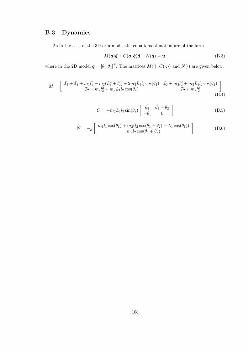
B.3 Dynamics
As in the case of the 3D arm model the equations of motion are of the form
M(q)q + C(q, q)q + N(q) = u, (B.3)
where in the 2D model q = [θ1 θ2]T . The matrices M(·), C(·, ·) and N(·) are given below.
M =
[I1 + I2 + m1l
21 + m2(L
21 + l22) + 2m2L1l2 cos(θ2) I2 + m2l
22 + m2L1l2 cos(θ2)
I2 + m2l22 + m2L1l2 cos(θ2) I2 + m2l
22
]
(B.4)
C = −m2L1l2 sin(θ2)
[θ2 θ1 + θ2
−θ1 0
]
(B.5)
N = −g
[m1l1 cos(θ1) + m2(l2 cos(θ1 + θ2) + L1 cos(θ1))
m2l2 cos(θ1 + θ2)
]
(B.6)
108