University of California, Merced Professor Jason Lee

EC� 121-Money and Banking

Chapter 5 Lecture �otes

I. Introduction

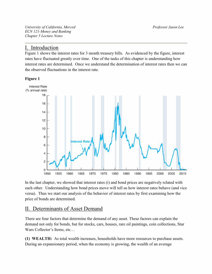
Figure 1 shows the interest rates for 3 month treasury bills. As evidenced by the figure, interest

rates have fluctuated greatly over time. One of the tasks of this chapter is understanding how

interest rates are determined. Once we understand the determination of interest rates then we can

the observed fluctuations in the interest rate.

Figure 1

In the last chapter, we showed that interest rates (i) and bond prices are negatively related with

each other. Understanding how bond prices move will tell us how interest rates behave (and vice

versa). Thus we start our analysis of the behavior of interest rates by first examining how the

price of bonds are determined.

II. Determinants of Asset Demand

There are four factors that determine the demand of any asset. These factors can explain the

demand not only for bonds, but for stocks, cars, houses, rare oil paintings, coin collections, Star

Wars Collector’s Items, etc…

(1) WEALTH: As total wealth increases, households have more resources to purchase assets.

During an expansionary period, when the economy is growing, the wealth of an average

household increases. During a recession, when the economy is contracting, the wealth of the

average household falls.

Key Point: An increase in wealth, will increase the demand for an asset, holding all else

constant.

(2) EXPECTED RETUR): The expected return is the rate of return of an asset relative to

alternative assets.

Consider the following example. Suppose that there are only two assets available for an

investor: shares of Google Stock and shares of Facebook Stock. Assume that initially both

stocks had a rate of return of 10%. Suddenly, Google has some good news which causes its

expected return to increase to 20%, while Facebook remains at 10%. Since, Google now has a

higher expected return, we would expect more investors to demand Google shares, thus the

demand for Google stock will increase. Notice that even though the rate of return of Facebook

has not change, there will be less demand for Facebook stock. The reason being is that the

expected return relative to Google of Facebook has fallen.

Key Point: An increase in expected return of an asset, relative of alternative assets, will

increase demand for the asset, holding all else constant.

(3) RISK: Suppose you were given a choice:

You could play a game where you flip a coin. If the coin turns up heads then you will receive

$200,000 but if the coin turns up tails you get $0.

Alternatively, you can select to receive $100,000.

Which would you choose? Although both options will give you the same expected return of

$100,000, most individuals will choose to take the $100,000 for certain. This indicates that

most people are what we call risk-averse, that is individuals try to avoid risk.

Like the scenario above, given a choice between two assets that offer the same expected return,

most individuals will choose the asset that is less risky.

Key Point: If the risk of an asset falls relative to that of alternative assets, then the demand

for that asset will increase, holding all else constant.

(4) LIQUIDITY: Recall that liquidity measures how quickly an asset can be converted to cash.

If the reason one holds assets is to make future purchases of goods and services, then having an

asset that is relatively liquid will be of some importance. An asset may be considered more

attractive if it is easier to sell.

Key Point: The more liquid an asset, the greater the demand for that asset, holding all else

constant.

Definition: The Theory of Portfolio Choice states that demand for an asset is positively related

to wealth, expected return and liquidity. Demand for an asset is negatively related to risk.

III. Bond Market

Now that we have some basic understanding on how the demand for assets are determine, we can

turn our attention to bonds. In particular, we are interested in how the price of a bond is

determined. It turns out that the price of a bond is determined the same way as any other good or

service: through supply and demand.

A. Demand Curve for Bonds

For simplicity, assume that we are discussing a one-year discount bond. We know from Ch.4

that the price of the one year discount bond is simply:

)1( i

FVPV

+= We showed in Chapter 4 how the yield-to-maturity is just the following:

PV

PVFVi

−=

Since there is no coupon payment, and that the price next year is simply the face value of the

bond, the formula for the yield-to-maturity of a discount bond is also the rate of return.

Thus the rate of return for a one-year discount bond = yield to maturity.

Suppose that we have a one-year discount bond with a face value of $1000 and an initial

purchase price of $950. Calculate the yield-to-maturity.

%3.5950$

950$1000$=

−=i

Assume that at that level of interest rates (expected return) that $50 billion on this bond is

demanded.

Now consider what would happen to the yield-to-maturity if the purchase price of the bond fell

to $900. Calculate the yield-to-maturity. Since the price of the bond fell, it must be the case that

the interest rate must be higher since they are negatively related with each other.

%1.11900$

900$1000$=

−=i

As the price fell, the interest rate has risen. Since for a one-year discount bond the yield-to-

maturity and rate of return are equivalent, then as the price of a bond falls, the rate of return rises.

We know from the theory of portfolio choice that the demand for an asset rises as the expected

rate of return increases. Thus at i = 11.1%, demand for bonds must be greater than $50 billon.

Assume that at 11.1%, $100 billion is demanded.

Figure 2, illustrates the different combination of bond prices and quantity of bonds demanded.

Figure 2

We can repeat this process for a series of different prices, but the end result will still be the same.

The demand for bonds (Bd) is a downward sloping curve. The demand curve states that at a

lower bond price (or equivalently at a higher interest rate), the quantity of bonds demanded will

be higher.

B. Supply Curve for Bonds

Let us return to our original one-year discount bond. Suppose that the price of the discount bond

is $750.

The yield-to-maturity (or the expected rate of return) will be %3.33750$

750$1000$=

−=i

At a bond price of $750, the cost of borrowing for firms is 33.3%. Suppose that at this very high

interest rate, the level of borrowing that the government (or firms) wish to undertake will be

relatively modest. Assume that the government wishes only to borrow (issue) $100 billion in

bonds at that price.

What if the price of the bond rises to $900? We saw that at a price of $900, the rate of return of

the one-year discount bond is 11.1%. Thus if the price of the bond rises to $900, the cost of

borrowing to the government or firms will fall significantly. Since the cost of borrowing is

lower, the government will be more willing to borrow (issue bonds) than they were before.

Suppose that at a bond price of $900, the government is willing to borrow $400 billion. We can

illustrate this in Figure 3.

Figure 3

The supply curve for bonds (Bs) is upward sloping, as the price increases, the quantity supplied

of bonds will also increase.

C. Market Equilibrium for Bonds

Not surprisingly, the price of a bond is found where the market demand for bonds (Bd) is equal to

the market supply for bonds (Bs). In equilibrium Bd = Bs.

Figure 4 shows the market equilibrium situation.

Figure 4

Note that if the bond price is above the market equilibrium (interest rate is below the equilibrium

interest rate) then we have a case where the amount of bonds issued is greater than the demand

for bonds. When (Bs > Bd) this is called excess supply. In order to attract buyers, bond issuers

may start lowering prices thus there is downward pressure on bond prices until the market

reaches equilibrium.

Conversely, when the bond price is below the market equilibrium (interest rate is above the

equilibrium interest rate) then we have a case where the amount of bonds issued is less than

demand for bonds. When (Bs < Bd) this is called excess demand. Not all buyers are able to

purchase bonds, so they start bidding up the price until the mark

IV. Changes in the Bond Market

A. Changes in the Demand for Bonds

Key Point: A change in the price of a bond (or equivalently a change in the interest rate)

will cause movement along the demand curve for bonds. A change in any other

determinant of demand (wealth, expected return, risk, or liquidity) will cause a shift in the

demand curve.

(1) An increase in demand will shift the bond demand curve to the right.

(2) A decrease in demand will shift the bond demand curve to the left.

Let us consider some scenarios in which the demand for bonds will shift.

Example #1: Recession

Suppose an economy enters into a recession. In a recession, output falls and therefore the wealth

of the average individual will also fall. According to the theory of portfolio choice, the demand

for assets (including bonds) should fall. This is illustrated in Figure 5.

Figure 5

In Figure 5, suppose that the initial price of the bond is at P0 and at that price Q0 amount of bonds

will be demanded. A recession will reduce the wealth of individuals causing them to reduce the

amount of bonds purchased. Note that the price of the bond has not changed. Thus at the same

price, P0, there is less demand for bonds (Q1). In the bond market we go from Point A to Point

B. At Point B, we are no longer on the initial demand curve, but at a point to the left of the

curve. As a result, it must be true that the bond demand must have shifted to the left.

Example #2: Change in Expected Interest Rates

Changes in expected interest rates will affect the return of bonds with a maturity greater than 1

year. Suppose that the expected interest rate is expected to fall soon. Since there is an inverse

relationship between bond prices and interest rate, the expected fall in interest rate should lead

one to expect that bond prices will soon rise. Higher bond prices will increase the expected

return for a bond. Thus we should expect that demand will shift to the right. This is shown in

Figure 6. Initially, we are at Point A, but an increase in expected return will cause investors to

demand more of a bond, even though prices remain unchanged today. It must be the case that

the curve has shifted to the right.

Figure 6

Example #3: Change in Expected Inflation

Inflation is the overall increase in prices. If there is an increase in expected inflation, then

individuals expect that the prices of all goods will increase. These goods include non-monetary

assets such as cars, houses, oil paintings etc… The expected increase in price will increase the

expected return of these non-monetary assets relative to bonds. Although bond prices have not

changed, the fact that cars and houses are more attractive relative to bonds will increase demand

for those assets and decrease demand for bonds. Graphically, it will be similar to Example #1.

To summarize: Factors that would cause the demand curve for bonds to shift to the right.

1. An increase in wealth

2. An decrease in the expected interest rate

3. A decrease in expected inflation

4. A decrease in the riskiness of bonds relative to other assets

5. An increase in the liquidity of bonds relative to other assets

The opposite factors would cause the demand curve for bonds to shift to the left.

B. Changes in the Supply for Bonds

There are three main factors that would cause the supply curve of bonds to shift.

(1) Changes in the expected profitability of investment opportunities/Changes in the

economy

If a firm finds that more of its proposed investment projects are suddenly profitable, then they

will want to use borrowed funds to undertake these projects. In order to access more funds they

will have to issue more bonds and thus the supply of bonds will increase. Profitable investment

opportunities themselves are tied to the state of the economy. If the economy is growing and

expanding then there are more profitable opportunities that are available and we would expect

the supply of bonds to increase in an expansion. On the other hand, if the economy is in a

recession, then it would be harder to find profitable opportunities and the supply of bonds may

decrease.

Consider the case of an expansion. During an expansion, as there is an increase in profitable

opportunities, firms will issue more bonds. Thus even though the price of bonds have not

change, there will be a greater supply. The supply curve will shift to the right.

Figure 7

(2) Changes in Expected Inflation

Consider what would happen if expected inflation increases.

Recall that the real interest rate measures the true cost of borrowing as it takes into account

inflation.

r = i – πe

An increase in expected inflation will lower the real interest rate. The true cost of borrowing will

decline, implying that it is cheaper for the borrower to borrow funds. Thus we would expect

firms and governments to issue more bonds.

An increase in expected inflation will shift the supply curve to the right as in Figure 7.

(3) Changes in Government Budget Deficits

Budget deficits occur when government tax revenue (T) is less that government spending (G).

When spending exceeds revenues, the government must make up the difference by borrowing.

Thus whenever deficits occur, the government issues more debt.

Consider a scenario where the government budget deficit is actually reduced. A fall in the deficit

means that less bonds will need to be issued by the government. Thus at any given price, the

supply of bonds will fall. This is illustrated in Figure 8.

Figure 8

To summarize: Factors that would cause the supply curve for bonds to shift to the right.

1. An expansion (increase in expected profitability of investment projects)

2. Increase in expected inflation

3. An increase in the government budget deficit

The opposite factors would cause the supply curve for bonds to shift to the left.

C. Interest Rate Determination

Now that we have studied the bond market, we are now ready to bring everything together and

analyze how shocks to the economy can affect the interest rate through the bond market.

Example: Recession

Q: What happens to interest rates in an economy as a result of a recession?

We know from earlier sections that a recession will have two effects on the bond market:

(1) The demand for bonds should fall as wealth declines. The demand curve will shift to the

left.

(2) The supply for bonds should also shift to the left, as the number of profitable investment

opportunities decline. Less investment projects will result in less bonds being issued.

Figure 9 illustrates both the supply curve and the demand curve shifting. From the graph it is

clear that the quantity of bonds will fall, but it is unclear what will happen to the price of bonds

(an hence what will happen to interest rates). Depending on the respective magnitudes of the

shift, the price of the bond may be higher, lower or equal to the initial price.

Figure 9

However, Figure 1 showed that during periods of recessions interest rates fall. Then it must be

the case that the price of bonds rise during a recession (in order to explain for the observed fall in

interest rates). In order for this to occur, the shift in supply must be greater than the shift in

demand. See Figure 10.

Figure 10

V. The Liquidity Preference Framework

A. Liquidity Preference Framework

Up to this point, we have seen that equilibrium in the bond market can be used to determine the

interest rate in the economy. However, there is an alternative model known as the liquidity

preference framework which shows the interest rates can be determined by equilibrium in the

money market. However, we can show that the bond market and money market can be linked.

In this model assume that there are only 2 assets available: money (currency) and bonds.

Assume that money as 0 rate of return, while bonds has a rate of return equal to the interest rate

(i).

Total wealth in the economy is held in just these two assets.

Total Wealth = BS + MS

It must also be true that people cannot buy more assets than are available to them. Thus, the total

demand for assets must equal the total supply of assets.

Bd + Md = BS + MS which can be rewritten as:

Bd - BS = MS - Md

Note that if the bond market is in equilibrium (Bd = BS), then the money market will also have to

be in equilibrium (MS = Md).

Key Point: If we equate money demand with money supply this is equivalent of equating

bond supply with bond demand. Liquidity Framework is equivalent to Loanable Funds

Framework.

B. The Money Market

The money market looks at the supply and demand for money. The point at which the supply of money

equals the demand for money is where interest rates are determined. Let’s take a brief look at the supply

and demand for money components.

Money Demand (Md)

The demand for money is intuitive since you make decisions everyday about how much currency you

wish to hold. One of the reasons we like to hold money is because we use it to conduct transactions of

goods and services. This is known as the transaction demand for money. However, the problem with

holding lots of currency is that you don’t earn any interest in holding cash. That can be a problem when

interest rates are high. If you could earn a 10% coupon rate by purchasing a bond, then keeping $1000 in

currency will cost you $100 over the course of the year. Thus the interest rate is the opportunity cost of

holding money. As interest rates increase, the opportunity cost of holding money increases and thus a

rational person will want to hold less money in cash. Conversely, if interest rates decrease then the

opportunity cost of holding money is lower and people might want to hold more money.

This idea of interest rate acting as the opportunity cost of holding money is captured by the money

demand curve. The money demand curve shows the negative relationship associated between the

interest rate and the amount of money held.

Figure 11

When interest rates change we move along the demand curve for money.

While interest rates are the primary determinant of the demand for money, there are other factors. Each

of these other factors will cause the demand curve to money to shift.

• Change in the price level: If prices of all goods were to suddenly double overnight, people will need twice the currency as before to purchase the same amount of goods. This will increase the demand for money. Figure 12 illustrates this change. Figure 12

Suppose we start at an initial point where the economy is

at interest rate io. At that interest rate the amount of

money demanded is at Mo. Now if the price level were to

double that’s going to increase the demand for money. At

the same interest rate of io, people are going to demand

more money (say M1). We’re no longer on our original

money demand curve, the curve must shift out to the right.

Thus an increase in the price level will increase the

demand for money. You can easily see that a decrease in

the price level will have the opposite effect.

• Change in the income level (Y): If suddenly you were to achieve the wealth of Oprah overnight, that will drastically affect your consumption patterns. As income goes up, people tend to purchase more goods and thus will need more currency in order to conduct these transactions. Thus as the income level increases money demand will increase and shift to the right. (Figure 12 illustrates this).

Money Supply (Ms)

The money supply in the economy is determined by the Federal Reserve independent of the interest rate.

We assume that the Fed chooses some given amount of money to supply to the economy. Thus the

money supply curve is vertical. If the Federal Reserve decides to increase the money supply, the money

supply curve will shift to the right. If the Federal Reserve decides to decrease the money supply, the

money supply curve will shift to the left.

Equilibrium (Ms = M

d)

Not surprisingly money market equilibrium is going to be where the money demand curve intersects the

money supply curve. Note that we can find equilibrium interest rate, where money supply and money

demand intersects.

Figure 13 shows the money market in equilibrium.

C. Determining Interest Rates in The Money Market|

Let us now turn our attention to see how changes in income, price levels and money supply can

affect the interest rates in an economy.

(1) Changes in the Income

Suppose that the economy is experiencing a recession. We saw, using the bond market, that both

the demand and supply of bonds would shift causing the quantity of bonds to fall, but the price of

bonds to be ambiguous. We had to use observed data to conclude that bond prices must rise in

order to explain the fall in interest rates.

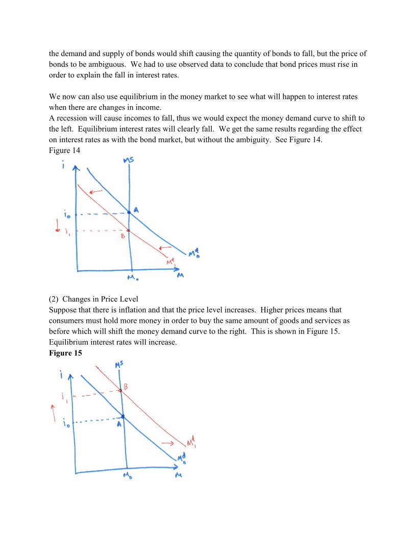
We now can also use equilibrium in the money market to see what will happen to interest rates

when there are changes in income.

A recession will cause incomes to fall, thus we would expect the money demand curve to shift to

the left. Equilibrium interest rates will clearly fall. We get the same results regarding the effect

on interest rates as with the bond market, but without the ambiguity. See Figure 14.

Figure 14

(2) Changes in Price Level

Suppose that there is inflation and that the price level increases. Higher prices means that

consumers must hold more money in order to buy the same amount of goods and services as

before which will shift the money demand curve to the right. This is shown in Figure 15.

Equilibrium interest rates will increase.

Figure 15

(3) Changes in Money Supply

An increase in the money supply will cause the money supply curve to shift to the right. As

shown in Figure 16 this will cause the equilibrium interest rate to fall.

Figure 16

D. Money Supply and the Interest Rate

In Figure 16, we saw that an increase in money supply will cause the money supply curve to shift

to the left, causing the equilibrium interest rate to fall. The fall in interest rate as a result of the

increase in money supply in the money market is known as the liquidity effect.

There are some critics, however, that argue that an increase in money supply has other effects on

the economy which would actually make interest rates increase. If these other effects were large

enough, they may outweigh, the liquidity effect and cause interest rates to rise. These effects

include:

(1) Income Effect: An increase in money supply is an expansionary monetary policy designed

to stimulate the economy. Over time, output levels should increase as a result of higher money

supply (we will discuss this in more detail later in the course). An expansion in the economy

will lead to higher incomes which should cause money demand to increase thereby raising the

interest rate (see Figure 15).

(2) Price-Level Effect: Again, we will discuss later in the course, that a consequence of

increasing the money supply is that prices in the economy will increase. One reason is that as

incomes increase due to the expansion, there is increase demand for goods and services which

push up prices. Higher prices will result in higher demand for money in order to conduct

transactions, thus the interest rate may rise.

(3) Expected-Inflation Effect: A final consequence of higher money supply, is that individuals

may form higher expectations concerning inflation. The initial increase in prices due to the

price-level effect, may cause some to believe that inflation will also be higher in the future.

According to our analysis of the bond market, higher expected inflation will lead to higher

interest rates. The difference between expected inflation and price-level effect, is that the price

level effect persists, while expected inflation effect is only temporary.

Consider two scenarios:

In the first scenario (depicted in Figure 17), the liquidity effect outweighs the other effects

(income, price-level and expected-inflation effects). Thus in Figure 17, suppose that the money

supply increases at time T. The result is an immediate fall in interest rates as a consequence of

the liquidity effect. Over time the other effects begin to have an impact and start raising interest

rates, but since the liquidity effect is stronger, the end result is that the interest rate will be lower

than its initial level.

Key Point: If the liquidity effect dominates, then increasing money supply will lower

interest rates.

Figure 17

In the second scenario (depicted in Figure 18), the liquidity effected is outweighed by the other

effects. Consider what would happen if money supply increased at time T. As before, this will

result in an immediate fall in interest rates as the liquidity effect takes effect. However, over

time, the income, price-level and expected inflation effects begin to dominate and push up

interest rates. In the end, the interest rate is actually above the initial interest rate.

Key Point: If the liquidity effect is dominated, then increasing the money supply will

increase the interest rates.

Figure 18

Which scenario is most likely? Well look at the empirical data in Figure 19. We can see periods

where increases in the money supply actually led to increases in the interest rates. This would

imply that the income, price-level, and expected inflation effects outweigh the liquidity effect.

Figure 19