cim-earth: philosophy, models, and case studiestmunson/papers/cim-earth.pdf · cim-earth:...

ARGONNE NATIONAL LABORATORY9700 South Cass AvenueArgonne, Illinois 60439

CIM-EARTH:Philosophy, Models, and Case Studies

Joshua Elliott, Ian Foster, Kenneth Judd, Elisabeth Moyer, and Todd Munson

Mathematics and Computer Science Division

Preprint ANL/MCS-P1710-1209

February 2010

Contents

1 Introduction 1

2 Philosophy 3

3 Computable General Equilibrium Models 53.1 Calibrated Share Model . . . . . . . . . . . . . . . . . . . . . . . . . . . . . 6

3.1.1 Industries . . . . . . . . . . . . . . . . . . . . . . . . . . . . . . . . . 63.1.2 Consumers . . . . . . . . . . . . . . . . . . . . . . . . . . . . . . . . . 83.1.3 Markets . . . . . . . . . . . . . . . . . . . . . . . . . . . . . . . . . . 93.1.4 Calibration . . . . . . . . . . . . . . . . . . . . . . . . . . . . . . . . 9

3.2 Taxes and Subsidies . . . . . . . . . . . . . . . . . . . . . . . . . . . . . . . . 103.2.1 Ad Valorem and Excise Taxes . . . . . . . . . . . . . . . . . . . . . . 103.2.2 Production Taxes . . . . . . . . . . . . . . . . . . . . . . . . . . . . . 103.2.3 Income Taxes . . . . . . . . . . . . . . . . . . . . . . . . . . . . . . . 103.2.4 Import and Export Duties . . . . . . . . . . . . . . . . . . . . . . . . 113.2.5 Carbon Taxes . . . . . . . . . . . . . . . . . . . . . . . . . . . . . . . 113.2.6 Endogenous Tax Rates . . . . . . . . . . . . . . . . . . . . . . . . . . 12

3.3 Myopic Dynamic Models . . . . . . . . . . . . . . . . . . . . . . . . . . . . . 133.4 Computational Framework . . . . . . . . . . . . . . . . . . . . . . . . . . . . 13

4 Dynamic Stochastic Models 154.1 Optimal Growth Problems . . . . . . . . . . . . . . . . . . . . . . . . . . . . 154.2 Dynamic Programming . . . . . . . . . . . . . . . . . . . . . . . . . . . . . . 164.3 Parallelization . . . . . . . . . . . . . . . . . . . . . . . . . . . . . . . . . . . 18

5 Case Studies 185.1 CIM-EARTH CGE Model . . . . . . . . . . . . . . . . . . . . . . . . . . . . 18

5.1.1 Regions and Industries . . . . . . . . . . . . . . . . . . . . . . . . . . 185.1.2 Production Functions . . . . . . . . . . . . . . . . . . . . . . . . . . . 195.1.3 Dynamic Trajectories . . . . . . . . . . . . . . . . . . . . . . . . . . . 215.1.4 Carbon Policy Study . . . . . . . . . . . . . . . . . . . . . . . . . . . 23

5.2 Parallel Stochastic Optimal Growth Problems . . . . . . . . . . . . . . . . . 24

6 Future Extensions 26

CIM-EARTH:Philosophy, Models, and Case Studies∗

Joshua Elliott† Ian Foster‡ Kenneth Judd§

Elisabeth Moyer¶ Todd Munson‖

February 15, 2010

Abstract

General equilibrium models have been used for decades to obtain insights into theeconomic implications of policies and decisions. Such models offer a treatment of hu-man behavior grounded in economic theory that also permits the integration of physicalconstraints on human activities. In this paper, we discuss our Community IntegratedModel of Economic and Resource Trajectories for Humankind (CIM-EARTH), includ-ing a justification of our open-source philosophy and details of our computable generalequilibrium and dynamic stochastic models. Case studies on the international conse-quences of unilateral carbon policy and solving stochastic optimal growth problems inparallel are used to illustrate the use of these models.

1 Introduction

Computable general equilibrium (CGE) models (Johansen, 1960, Robinson, 1991, Sue Wing,2004) and their stochastic counterparts, dynamic stochastic general equilibrium (DSGE)

∗This work was supported by grants from the MacArthur Foundation and the University of ChicagoEnergy Initiative, and by the Office of Advanced Scientific Computing Research, Office of Science, U.S.Department of Energy, under Contract DE-AC02-06CH11357. This report was prepared as an account ofwork sponsored by an agency of the United States Government. Neither the United States Government norany agency thereof, nor UChicago Argonne, LLC, nor any of their employees or officers, makes any warranty,express or implied, or assumes any legal liability or responsibility for the accuracy, completeness, or usefulnessof any information, apparatus, product, or process disclosed, or represents that its use would not infringeprivately owned rights. Reference herein to any specific commercial product, process, or service by tradename, trademark, manufacturer, or otherwise, does not necessarily constitute or imply its endorsement,recommendation, or favoring by the United States Government or any agency thereof. The views andopinions of document authors expressed herein do not necessarily state or reflect those of the United StatesGovernment or any agency thereof, Argonne National Laboratory, or UChicago Argonne, LLC.†Computation Institute, U. Chicago and Argonne National Laboratory, email: [email protected]‡Computation Institute, U. Chicago and Argonne National Laboratory, email: [email protected]§Hoover Institute and U. Chicago Economics, email: [email protected]¶U. Chicago Geophysics, email: [email protected]‖Computation Institute, U. Chicago and Argonne National Laboratory, email: [email protected]

1

models (Del Negro and Schorfheide, 2003), form the backbone of policy analysis programsaround the world and have been used for decades to obtain insights into the economicimplications of policies (Bhattacharyya, 1996, Shoven and Whalley, 1984, de Melo, 1988).Indeed, hundreds of such models have been built since their introduction (Devarajan andRobinson, 2002, Conrad, 2001). By computing market prices and the levels of supply anddemand subject to productions constraints, taxes, and transportation costs, these modelscan be used to explore such policy-relevant questions as the impact of new tax policies orincreased fossil energy costs on consumers. Moreover, these models form a core componentwhen studying the interaction between economic activity and the Earth system with anintegrated assessment model (IAM) (Dowlatabadi and Morgan, 1993, Weyant, 2009).

Despite successes, however, these economic models have limitations (Scrieciu, 2007).Models may not incorporate the industrial or process detail required to answer questionsof interest; costs estimates from different models often differ considerably (Vuuren et al.,2009, Weyant, 1999, 2006, Friedlingstein et al., 2006, Lee, 2006); and little or no quan-tification of the uncertainty inherent in their estimates is performed. To understand thedistributional impacts of a carbon emission policy, for example, one needs to represent theindustries, regions, and income groups that may be affected and the complex interactionsbetween different policies in different regions.

Many limitations of current economic models are due to computational and methodologi-cal constraints that can be overcome by leveraging recent advances in computer architecture,numerical methods, and economics research. For example, contemporary models use mathe-matical formulations, numerical methods, and computer systems that restrict the size of themodels that can be solved in a reasonable time to a few tens of thousands of equations. Thus,it becomes impractical to add important detail such as increased industrial, geographic, ortemporal resolution; capital vintages; overlapping generations; or stochastic dynamics. Yetmore modern formulations and solvers, and more powerful computer systems, offer the po-tential to solve systems of equations that are several orders of magnitudes larger. Thus, wecan in principle create models that encompass more details of importance to decision makersand characterize the model uncertainty. These results can then be used to identify policiesthat are robust to model uncertainty.

Motivated by these considerations, we are developing a new modeling framework: theCommunity Integrated Model of Economic And Resource Trajectories for Humankind (CIM-EARTH). Our goal is to facilitate and encourage the creation, execution, and testing of neweconomic models with significantly greater fidelity and sophistication than is the norm to-day. We envision the framework as combining (a) a high-level programming notation thatpermits the convenient formulation of a wide range of models with different purposes andcharacteristics; (b) a flexible implementation that permits the efficient solution of these mod-els using the most advanced numerical methods and, where appropriate, high-performancecomputer systems; and (c) a suite of associated tools for parameter estimation, uncertaintyquantification, and model validation.

We seek not only to provide access to better economic formulations and numerical meth-ods but to also encourage the development and use of open models, that is, models that areboth made freely available to all under terms that permit modification and redistributionand that are designed to facilitate study, modification, application, contribution, and redis-tribution by others. Open models play an important role in encouraging the application of

2

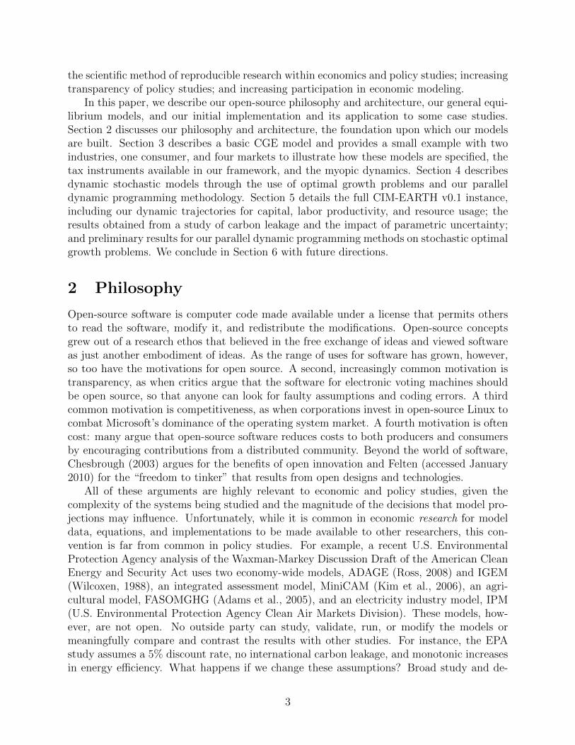
the scientific method of reproducible research within economics and policy studies; increasingtransparency of policy studies; and increasing participation in economic modeling.

In this paper, we describe our open-source philosophy and architecture, our general equi-librium models, and our initial implementation and its application to some case studies.Section 2 discusses our philosophy and architecture, the foundation upon which our modelsare built. Section 3 describes a basic CGE model and provides a small example with twoindustries, one consumer, and four markets to illustrate how these models are specified, thetax instruments available in our framework, and the myopic dynamics. Section 4 describesdynamic stochastic models through the use of optimal growth problems and our paralleldynamic programming methodology. Section 5 details the full CIM-EARTH v0.1 instance,including our dynamic trajectories for capital, labor productivity, and resource usage; theresults obtained from a study of carbon leakage and the impact of parametric uncertainty;and preliminary results for our parallel dynamic programming methods on stochastic optimalgrowth problems. We conclude in Section 6 with future directions.

2 Philosophy

Open-source software is computer code made available under a license that permits othersto read the software, modify it, and redistribute the modifications. Open-source conceptsgrew out of a research ethos that believed in the free exchange of ideas and viewed softwareas just another embodiment of ideas. As the range of uses for software has grown, however,so too have the motivations for open source. A second, increasingly common motivation istransparency, as when critics argue that the software for electronic voting machines shouldbe open source, so that anyone can look for faulty assumptions and coding errors. A thirdcommon motivation is competitiveness, as when corporations invest in open-source Linux tocombat Microsoft’s dominance of the operating system market. A fourth motivation is oftencost: many argue that open-source software reduces costs to both producers and consumersby encouraging contributions from a distributed community. Beyond the world of software,Chesbrough (2003) argues for the benefits of open innovation and Felten (accessed January2010) for the “freedom to tinker” that results from open designs and technologies.

All of these arguments are highly relevant to economic and policy studies, given thecomplexity of the systems being studied and the magnitude of the decisions that model pro-jections may influence. Unfortunately, while it is common in economic research for modeldata, equations, and implementations to be made available to other researchers, this con-vention is far from common in policy studies. For example, a recent U.S. EnvironmentalProtection Agency analysis of the Waxman-Markey Discussion Draft of the American CleanEnergy and Security Act uses two economy-wide models, ADAGE (Ross, 2008) and IGEM(Wilcoxen, 1988), an integrated assessment model, MiniCAM (Kim et al., 2006), an agri-cultural model, FASOMGHG (Adams et al., 2005), and an electricity industry model, IPM(U.S. Environmental Protection Agency Clean Air Markets Division). These models, how-ever, are not open. No outside party can study, validate, run, or modify the models ormeaningfully compare and contrast the results with other studies. For instance, the EPAstudy assumes a 5% discount rate, no international carbon leakage, and monotonic increasesin energy efficiency. What happens if we change these assumptions? Broad study and de-

3

CIM-EARTH framework

Component repository

Archive and libraries

Data repository

Emulators

Numerical libraries

PC Cluster Cloud Supercomputer

Meta-applications

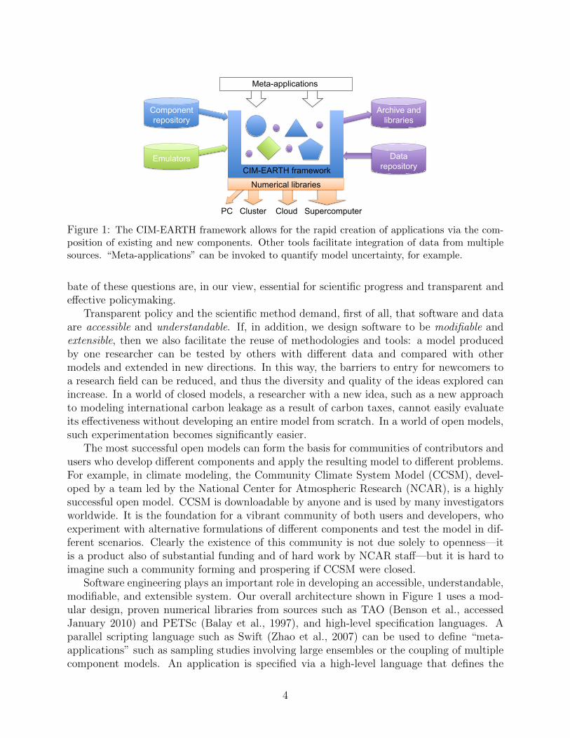
Figure 1: The CIM-EARTH framework allows for the rapid creation of applications via the com-position of existing and new components. Other tools facilitate integration of data from multiplesources. “Meta-applications” can be invoked to quantify model uncertainty, for example.

bate of these questions are, in our view, essential for scientific progress and transparent andeffective policymaking.

Transparent policy and the scientific method demand, first of all, that software and dataare accessible and understandable. If, in addition, we design software to be modifiable andextensible, then we also facilitate the reuse of methodologies and tools: a model producedby one researcher can be tested by others with different data and compared with othermodels and extended in new directions. In this way, the barriers to entry for newcomers toa research field can be reduced, and thus the diversity and quality of the ideas explored canincrease. In a world of closed models, a researcher with a new idea, such as a new approachto modeling international carbon leakage as a result of carbon taxes, cannot easily evaluateits effectiveness without developing an entire model from scratch. In a world of open models,such experimentation becomes significantly easier.

The most successful open models can form the basis for communities of contributors andusers who develop different components and apply the resulting model to different problems.For example, in climate modeling, the Community Climate System Model (CCSM), devel-oped by a team led by the National Center for Atmospheric Research (NCAR), is a highlysuccessful open model. CCSM is downloadable by anyone and is used by many investigatorsworldwide. It is the foundation for a vibrant community of both users and developers, whoexperiment with alternative formulations of different components and test the model in dif-ferent scenarios. Clearly the existence of this community is not due solely to openness—itis a product also of substantial funding and of hard work by NCAR staff—but it is hard toimagine such a community forming and prospering if CCSM were closed.

Software engineering plays an important role in developing an accessible, understandable,modifiable, and extensible system. Our overall architecture shown in Figure 1 uses a mod-ular design, proven numerical libraries from sources such as TAO (Benson et al., accessedJanuary 2010) and PETSc (Balay et al., 1997), and high-level specification languages. Aparallel scripting language such as Swift (Zhao et al., 2007) can be used to define “meta-applications” such as sampling studies involving large ensembles or the coupling of multiplecomponent models. An application is specified via a high-level language that defines the

4

type of model (deterministic or stochastic, myopic or forward looking), the size of the model(regions, industries, consumers, time periods), the details for the industries and consumers(production and utility functions) and their parametrization (elasticities of substitution),and the coupling with other system components. In defining this language, we build onexperience with general mathematical programming systems such as AMPL (Fourer et al.,2003) and GAMS (Brooke et al., 1988) and systems designed more specifically to supportCGE modeling such as GEMPACK (Harrison and Pearson, 1994) and MPSGE (Rutherford,1999). Each system is widely used, but has limitations. MPSGE models, for example, cannotinclude stochastic dynamics. Our tools currently compile an application specification to anAMPL model that can be read, modified, and solved.

Establishing a fully successful culture of open models in economics research and poli-cymaking is a complex issue, and we recognize that real success in open modeling requiresmore than good software engineering. Above all, it requires a transformation of disciplinaryculture, so that researchers become comfortable producing research using models that havebeen constructed by many contributors, funding agencies become comfortable paying for thedevelopment and sustenance of such models, and appointment and promotion committeesbecome comfortable with interdisciplinary papers having many authors. These changes haveoccurred in other disciplines, such as climate science, and we hope to set an example ineconomic modeling that others can follow.

3 Computable General Equilibrium Models

Computable general equilibrium models determine prices and quantities over time for com-modities such that supply equals demand for each good (Ballard et al., 1985, Ginsburgh andKeyzer, 1997, Scarf and Shoven, 1984). Such models have the following features:

• Many industries that hire labor, rent capital, and buy inputs to produce outputs. Eachindustry chooses a feasible production schedule to maximize its profit, the revenuereceived by selling its outputs minus the costs of producing them.

• Many consumers that choose what to buy and how much to work subject to theconstraint that purchases cannot exceed income. Each consumer chooses a feasibleconsumption schedule to maximize his happiness as measured by a utility function.

• Many markets where producers and consumers trade that set wage rates and commod-ity prices to “clear” the markets. In particular, if the price of a commodity is positive,then supply must equal demand.

The primary modeling challenge is estimating the production and utility functions thatcharacterize the physical and economic processes constraining the supply and demand de-cisions of industries and consumers. For our CGE models, we use constant elasticity ofsubstitution (CES) production and utility functions. We detail the calibrated share modelusing a simple example to fix notation and discuss the inclusion of taxes and subsidies. Wethen describe the myopic dynamic model and our computational framework and numericalmethods.

5

3.1 Calibrated Share Model

Calibrated constant elasticity of substitution functions (Boehringer et al., 2003) have theform

y

y=

(∑i

θi

(γixixi

)σ−1σ

) σσ−1

,

where yy

is the ratio between the output of the industry to a base year value, xixi

are theratios of the input commodities to their base year values, γi are the efficiency units thatdetermine how effectively these factors can be used, θi are the share parameters with θi > 0and

∑i θi = 1, and σ controls the degree to which the inputs can be substituted for one

another. When σ = 0, we obtain the Leontief production function

y

y= min

i

{γixixi

},

in which the inputs are perfectly complementary; an increase in output requires an increasein all inputs. When σ = 1, we obtain the Cobb-Douglas production function

y

y=∏i

(γixixi

)θi.

These functions are typically combined in a nested fashion where each nest describes thesubstitutability among commodity bundles.

The optimization problems solved by the industries and consumers and the market clear-ing conditions are then expressed in terms of the dimensionless variables

p =p

p, x =

x

x, y =

y

y.

These dimensionless variables represent the change in prices and quantities from their base-year values. The share parameters are then calibrated so that in the base year p = 1, x = 1,and y = 1. That is, we choose shares that replicate the base-year revenue and expendituredata.

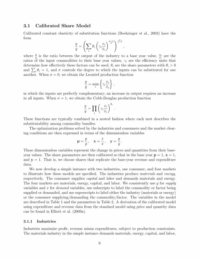
We now develop a simple instance with two industries, one consumer, and four marketsto illustrate how these models are specified. The industries produce materials and energy,respectively. The consumer supplies capital and labor and demands materials and energy.The four markets are materials, energy, capital, and labor. We consistently use y for supplyvariables and x for demand variables, use subscripts to label the commodity or factor beingsupplied or demanded, and use superscripts to label either the industry (materials or energy)or the consumer supplying/demanding the commodity/factor. The variables in the modelare described in Table 1 and the parameters in Table 2. A derivation of the calibrated modelusing expenditure and revenue data from the standard model using price and quantity datacan be found in Elliott et al. (2009a).

3.1.1 Industries

Industries maximize profit, revenue minus expenditures, subject to production constraints.The materials industry in the simple instance demands materials, energy, capital, and labor,

6

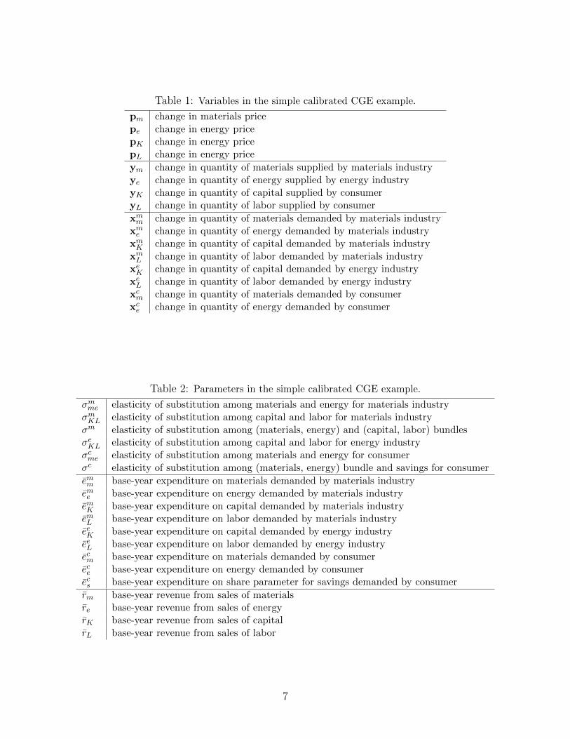
Table 1: Variables in the simple calibrated CGE example.

pm change in materials pricepe change in energy pricepK change in energy pricepL change in energy price

ym change in quantity of materials supplied by materials industryye change in quantity of energy supplied by energy industryyK change in quantity of capital supplied by consumeryL change in quantity of labor supplied by consumer

xmm change in quantity of materials demanded by materials industryxme change in quantity of energy demanded by materials industryxmK change in quantity of capital demanded by materials industryxmL change in quantity of labor demanded by materials industryxeK change in quantity of capital demanded by energy industryxeL change in quantity of labor demanded by energy industryxcm change in quantity of materials demanded by consumerxce change in quantity of energy demanded by consumer

Table 2: Parameters in the simple calibrated CGE example.

σmme elasticity of substitution among materials and energy for materials industryσmKL elasticity of substitution among capital and labor for materials industryσm elasticity of substitution among (materials, energy) and (capital, labor) bundlesσeKL elasticity of substitution among capital and labor for energy industryσcme elasticity of substitution among materials and energy for consumerσc elasticity of substitution among (materials, energy) bundle and savings for consumer

emm base-year expenditure on materials demanded by materials industryeme base-year expenditure on energy demanded by materials industryemK base-year expenditure on capital demanded by materials industryemL base-year expenditure on labor demanded by materials industryeeK base-year expenditure on capital demanded by energy industryeeL base-year expenditure on labor demanded by energy industryecm base-year expenditure on materials demanded by consumerece base-year expenditure on energy demanded by consumerecs base-year expenditure on share parameter for savings demanded by consumer

rm base-year revenue from sales of materialsre base-year revenue from sales of energyrK base-year revenue from sales of capitalrL base-year revenue from sales of labor

7

EnergyMaterials LaborCapital

Output

Figure 2: Basic nest for production function.

while the energy industry demands only capital and labor. In particular, the materialsindustry solves the optimization problem

maxym≥0,xmi ≥0

rmpmym − emmpmxmm − eme pexme − emKpKxmK − emLpLxmL

s.t. ym ≤(θmKL(xmKL)ρ

m+ θmme(x

mme)

ρm) 1ρm

xmKL ≤(θmK(xmK)ρ

mKL + θmL (xmL )ρ

mKL

) 1ρmKL

xmme ≤(θmm(xmm)ρ

mme + θme (xme )ρ

mme) 1ρmme ,

(1)

where ρm = σm−1σm

, ρmKL =σmKL−1

σmKL, and ρmme = σmme−1

σmme. The production function constraints

in (1) are depicted graphically by the tree structure shown in Figure 2, with each noderepresenting a production function with its own elasticity of substitution that aggregatesthe inputs from below into a commodity bundle. The root node then aggregates the twointermediate commodity bundles into the total materials output.

The energy industry solves a similar, but simpler optimization problem since it demandsonly capital and labor:

maxye≥0,xei≥0

repeye − eeKpKxeK − eeLpLxeL

s.t. ye ≤(θeK(xeK)ρ

eKL + θeL(xmL )ρ

mKL

) 1ρmKL .

3.1.2 Consumers

Consumers maximize their individual utility subject to a budget constraint; expenditurescannot exceed income. The consumer in the simple instance demands materials and energy,while supplying capital and labor. The supply of capital and labor is an endowed commodity;the consumer begins the period with a certain labor endowment and capital accumulated

EnergyMaterials

Utility

Savings

Figure 3: Basic nest for utility function.

8

from past savings. In particular, the consumer solves the optimization problem

max0≤ycj≤1,xci≥0

xc

s.t. xc ≤(θcme(x

cme)

ρc + θcS(xcS)ρc) 1

ρc

xcme ≤(θcm(xcm)ρ

cme + θce(x

ce)ρcme) 1ρcme

ecSxcS + ecmpmx

cm + ecepex

ce ≤ rcKpKy

cK + rcLpLy

cL + Πm + Πe ,

(2)

where ρc = σc−1σc

, ρcme = σcme−1σcme

, and Πm and Πe are the materials and energy industryprofits returned to the consumer as a dividend, respectively. The savings demanded by theconsumer, xcS, is necessary for myopic dynamic models to approximate the future utility ofconsumption. These savings are enter the economy as capital in the next time step. Inpractice, we choose σc to be one so that the CES function aggregating savings and the(materials, energy) bundle reduces to the Cobb-Douglas function, which implies that a fixedshare of consumer income goes to savings each year. The utility function constraints in (2)are depicted graphically by the tree structure shown in Figure 3.

3.1.3 Markets

The market clearing conditions are as follows:

0 ≤ pm ⊥ rmym ≥ emmxmm + ecmx

cm

0 ≤ pe ⊥ reye ≥ eme xme + ecex

ce

0 ≤ pL ⊥ rLyL ≥ emL xmL + eeLx

eL

0 ≤ pK ⊥ rKyK ≥ emKxmK + eeKx

eK .

The complementarity condition signified by ⊥ implies that one of the two inequalities ineach expression must be saturated. That is, either supply equals demand and the price isnonnegative, or supply exceeds demand and the price is zero. In particular, a zero pricemeans that the market for the good or factor collapses.

3.1.4 Calibration

Assuming revenues equal expenditures in all industry objective functions, consumer budgetconstraints, and market clearing conditions, we can choose values for the share parametersso that p = 1, y = 1, and x = 1 solves the problem. That is, the prices and quantities donot deviate from their base-year levels. This process of choosing the share parameters basedon base-year data is referred to as calibration to a base year. In particular, by choosing

θmm = emmemm+eme

θeK =eeK

eeK+eeL

θme = emeemm+eme

θeL =eeL

eeK+eeL

θmK =emK

emK+emLθcK =

ecKecK+ecL

θmL =emL

emK+emLθcL =

ecLecK+ecL

θmKL =emKL

emKL+emmeθcme = ecme

ecme+ecS

θmme = emmeemme+e

mme

θcS =ecS

ecKL+ecS,

where emKL = emK + emL , emme = emm + eme , and ecKL = ecK + ecL, one can show that p = 1, y = 1,and x = 1 is a solution.

9

3.2 Taxes and Subsidies

Taxes are an important part of an economy and any CGE model. Import and export taxesplay an important role in determining the sizes of bilateral trade flows; domestic taxescan reallocate economic activity into more socially advantageous efforts; and environmentaltaxes can be levied to encourage carbon-neutral behaviors and slow the emission of CO2 andother harmful pollutants into the atmosphere. Here we detail how taxes are included in theproduction, consumption, and investment equations. Subsidies are simply a negative taxrate. Tax revenues are aggregated into region-specific tax accounts.

3.2.1 Ad Valorem and Excise Taxes

Each industry in the model pays a tax on the value of the goods and factors demanded. Sometaxes, such as the federal gasoline tax, are applied to volumes rather than value. These taxesmodify the expenditure terms in the optimization problems solved by the industries. Usingthe materials industry from the simple example, we calculate the expenditure on energyinputs as

((eme + sme )pe + tme )xme ,

where sme is the ad valorem tax expenditure and tme is the excise tax expenditure. Thedistinction between ad valorem and excise taxes matters only as the change in commodityprices stray from unity and the difference is strongly dependent on the excise tax expenditure.For example, if the price of a commodity taxed in the base year at 10% doubles, then thetax revenues will be off by approximately 5% if the incorrect tax representation is used.

3.2.2 Production Taxes

Production taxes are paid by industries on the goods they produce. Using the materialsindustry from the simple example, the revenue from materials production becomes

((rmm − smm)pm − tmm)ym ,

where smm and tmm are the ad valorem and excise tax expenditures, respectively. Exciseproduction taxes may be needed to study the effects of a producer-level carbon tax. Forexample, if one charges an emissions tax based on the amount of coal mined rather than theamount of coal burned to generate energy, then we would need an excise production tax onmined coal. While carbon may not be priced in this way, the analysis extends to this case.

3.2.3 Income Taxes

Income taxes are subtracted from the consumer incomes at the point of payment. Thesetaxes have the same form as production taxes but are levied on the consumer revenue terms.Using consumer capital from the simple example, we calculate the modified revenue term as

((rcK − scK)pK − tcK)yK ,

where scK and tcK are the ad valorem and excise tax expenditures, respectively. We note thatwhile excise taxes on labor and capital are not likely to be imposed, the modeling frameworkdoes not prevent their inclusion.

10

3.2.4 Import and Export Duties

For international trade, we treat domestic and imported goods as distinct products. Eachregion contains an importer for each commodity that buys goods internationally and sellsthem domestically. Because the importer inputs commodities from many regions, we need todistinguish between import and export duties, since the duties are paid at the destination ororigination points, respectively. That is, we must distribute the revenue to the correct region.Using the materials commodity from the simple example, we calculate the expenditures forthe materials importer in region r′ as((

ei,r′

m,r + si,r′

m,r + se,r′

m,r

)pm,r

)+ ti,r

′

m,r + te,r′

m,rxi,r′

m,r ,

where si,r′

m,r and ti,r′

m,r are the ad valorem and excise import duty amounts for materials imported

from region r, respectively, and se,r′

m,r and te,r′

m,r are the ad valorem and excise export dutyamounts for materials exported by region r.

3.2.5 Carbon Taxes

Carbon taxes are excise taxes placed on the inputs and outputs of producers and consumers.Since carbon emissions are free in most of the world, no data is typically available for industryexpenditures on carbon emissions in the base year and we need to compute the taxablecarbon emissions. Using the materials industry from the simple example, we calculate theexpenditure on energy with a carbon tax as

(eme pe + tme fme )xme ,

where tme is the tax rate per emissions unit and fme is the taxable base-year emissions unitsgenerated by the materials industry from the use of energy. The emissions factors for simplecarbon taxes are usually based on available energy use volume data.

Carbon taxes on imports and exports are also used for border-tax adjustments on emis-sions. Using the materials commodity from the simple example, we calculate the border-taxadjustment for the materials importer in region r′ as

(ei,r′

m,rpm,r + ti,r′

m,rfi,r′

m,r + te,r′

m,rfe,r′

m,r)xi,r′

m,r ,

where ti,r′

m,r and te,r′

m,r are the import and export duties per emissions unit, respectively, and

f i,r′

m,r and f e,r′

m,r are the taxable base-year emissions units for the materials importer. Exportduties are negative when the exporting country refunds the carbon taxes on their exports.

Measuring the emissions units in this case is hard given the difficult carbon accountingintroduced by the fact that the commodity in question may not be produced in the taxingregion. We calculate the carbon content by assuming conservation of carbon. Therefore,the carbon content of the output is the sum of the carbon content of the inputs used in theproduction processes

Cjr yjryjr =∑ir

Cir xjrirxjrir ,

where C∗ is the carbon content per unit of the commodity, ir is the set of commodities used inthe production of good jr, x

jrir

is the base-year volume of commodity i used in the production

11

of commodity j in region r, and yjr is the base-year volume of commodity j produced bythe industry in region r, and xjrir (t).

This expression is written in terms of quantities, whereas most available data is in termsof expenditures. Therefore, rather than compute the carbon content per commodity unit,we compute the total carbon budget for the industry measured in terms of the base-yearquantities. In particular, we make the substitution

fjr = Cjr yjr

to obtain the equivalent system

fjryjr =∑ir

firxjriryir

xjrir .

We typically do not know the base-year volumes xjrir and yir . In those cases where we doknow the volume data for the base year, however, we directly compute the ratio. In all othercases, we compute the ratio from available expenditure data,

xjriryir

=pir x

jrir

pir yir=ejrirRir

≡ Φjrir,

where the expenditure and revenue data for each industry, ejrir and Rir , respectively, areknown. Note that if the volume and expenditure data are consistent, the ratios computedfrom either will be identical. Therefore, we have

fjryjr =∑ir

firΦjrirxjrir . (3)

We estimate the total carbon budget fjr for each industry j in region r by solving thesystem of equations (3) for given Φ, x, and y. These amounts are then used in the carbontax computations. However, this system has more variables than equations due to the land,labor, and capital factors. In our model, we ignore the contribution of these factors to thecarbon content by fixing their amounts to zero. We are then left with a square system ofequations having zero as a solution. Therefore, we fix the carbon amounts for the energyindustries using energy volume data and standard conversion factors and solve the reducedsystem for the remaining emission factors.

3.2.6 Endogenous Tax Rates

Endogenous taxes rates are required to implement cap-and-trade policies. In this case, thetax rate is determined within the model so that the cap is not violated. We discuss anendogenous carbon emissions tax, but other endogenous taxes can be added to the model.The mechanism for setting the rate is to create a market for emissions having a fixed supply,with the price of emissions determined so that the demand does not exceed the supply.

In the simple example, an endogenous tax on the emissions from energy consumptionwould introduce the constraints

0 ≤ te ⊥ Fe ≥ fme xme + f cexce ,

12

where te is the endogenous tax rate on energy; Fe is the cap on emissions from energy; andfme and f ce are the taxable base year emissions units generated by the materials industry andconsumer from the use of energy, respectively. In a calibrated model having no endogenouscarbon tax in the base year, we set Fe = fme + f ce . Analysis of the entire CGE problemshows that the tax rate in the base year is then zero. That is, under a business-as-usualscenario, there is no tax. By using a fraction of the base-year emissions, a positive tax rateis obtained.

3.3 Myopic Dynamic Models

The simplest dynamic CGE models are myopic, in which the industries and consumerslook only at their current state and do not consider the future. In this case, we solvea sequence of static CGE models with dynamic trajectories for the factor endowments,efficiency units, and emission factors. The primary drivers of economic development arecapital accumulation, labor productivity, and resource usage. We use exogenous time-seriesforecasts of important economic drivers constructed by extrapolation from historical data,with forecasts constrained by physical restrictions such as expected fossil reserve availability.The construction of these trajectories is documented in Section 5.1.

3.4 Computational Framework

Because the optimization problems solved by the industries and consumers are convex intheir own variables and satisfy a constraint qualification, we can replace each with an equiv-alent complementarity problem obtained from the first-order optimality conditions by addingLagrange multipliers on the constraints. If we assume all functions are general constant elas-ticity of substitution functions, the first-order conditions for the material industry are

Πm ⊥ Πm + emmpmxmm + eme pex

me + emKpKx

mK + emLpLx

mL − rmpmym = 0

0 ≤ ym ⊥ λm − rmpm ≥ 0

0 ≤ xmKL ⊥ λmKL − θmKL(θmKL(xmKL)ρ

m+ θmme(x

mme)

ρm) 1ρm−1

(xmKL)ρm−1 λm ≥ 0

0 ≤ xmme ⊥ λmme − θmme(θmKL(xmKL)ρ

m+ θmme(x

mme)

ρm) 1ρm−1

(xmme)ρm−1 λm ≥ 0

0 ≤ xmK ⊥ emKpK − θmK(θmK(xmK)ρ

mKL + θmL (xmL )ρ

mKL

) 1ρmKL−1

(xmK)ρmKL−1 λmKL ≥ 0

0 ≤ xmL ⊥ emLpL − θmL(θmK(xmK)ρ

mKL + θmL (xmL )ρ

mKL

) 1ρmKL−1

(xmL )ρmKL−1 λmKL ≥ 0

0 ≤ xmm ⊥ emmpm − θmm(θmm(xmm)ρ

mme + θme (xme )ρ

mme) 1ρmme−1

(xmm)ρmme−1 λmme ≥ 0

0 ≤ xme ⊥ eme pe − θme(θmm(xmm)ρ

mme + θme (xme )ρ

mme) 1ρmme−1

(xme )ρmme−1 λmme ≥ 0

0 ≤ λm ⊥(θmKL(xmKL)ρ

m+ θmme(x

mme)

ρm) 1ρm − ym ≥ 0

0 ≤ λmKL ⊥(θmK(xmK)ρ

mKL + θmL (xmL )ρ

mKL

) 1ρmKL − xmKL ≥ 0

0 ≤ λmme ⊥(θmm(xmm)ρ

mme + θme (xme )ρ

mme) 1ρmme − xmme ≥ 0 ,

13

for the energy industry are

Πe ⊥ Πe + eeKpKxeK + eeLpLx

eL − repeye = 0

0 ≤ ye ⊥ λe − repe0 ≤ xeK ⊥ eeKpK − θeK

(θeK(xeK)ρ

eKL + θeL(xmL )ρ

mKL

) 1ρmKL−1

(xeK)ρeKL−1 λe ≥ 0

0 ≤ xeL ⊥ eeLpL − θeL(θeK(xeK)ρ

eKL + θeL(xmL )ρ

mKL

) 1ρmKL−1

(xeL)ρeKL−1 λe ≥ 0

0 ≤ λe ⊥(θeK(xeK)ρ

eKL + θeL(xmL )ρ

mKL

) 1ρmKL − ye ≥ 0 ,

and for the consumer are

0 ≤ xc ⊥ λc − 1 ≥ 0

0 ≤ xcme ⊥ λcme − θcme(θcme(x

cme)


ρc−1

(xcme)ρc−1 λc ≥ 0

0 ≤ xcS ⊥ ecSµc − θcS(θcme(x

cme)


ρc−1

(xcS)ρc−1 λc ≥ 0

0 ≤ xcm ⊥ ecmpmµc − θcm(θcm(xcm)ρ

cme + θce(x

ce)ρcme) 1ρcme−1

(xcm)ρcme−1 λcme ≥ 0

0 ≤ xce ⊥ ecepeµc − θce(θcm(xcm)ρ

cme + θce(x

ce)ρcme) 1ρcme−1

(xce)ρcme−1 λcme ≥ 0

0 ≤ ycK ≤ 1 ⊥ −rcKpKµc0 ≤ ycL ≤ 1 ⊥ −rcLpLµc0 ≤ λc ⊥

(θcme(x

cme)


ρc − xc ≥ 0

0 ≤ λcme ⊥(θcm(xcm)ρ

cme + θce(x

ce)ρcme) 1ρcme − xcme ≥ 0

0 ≤ µc ⊥ rcKpKycK + rcLpLy

cL − ecSxcS − ecmpmxcm − ecepexce + Πm + Πe ≥ 0 .

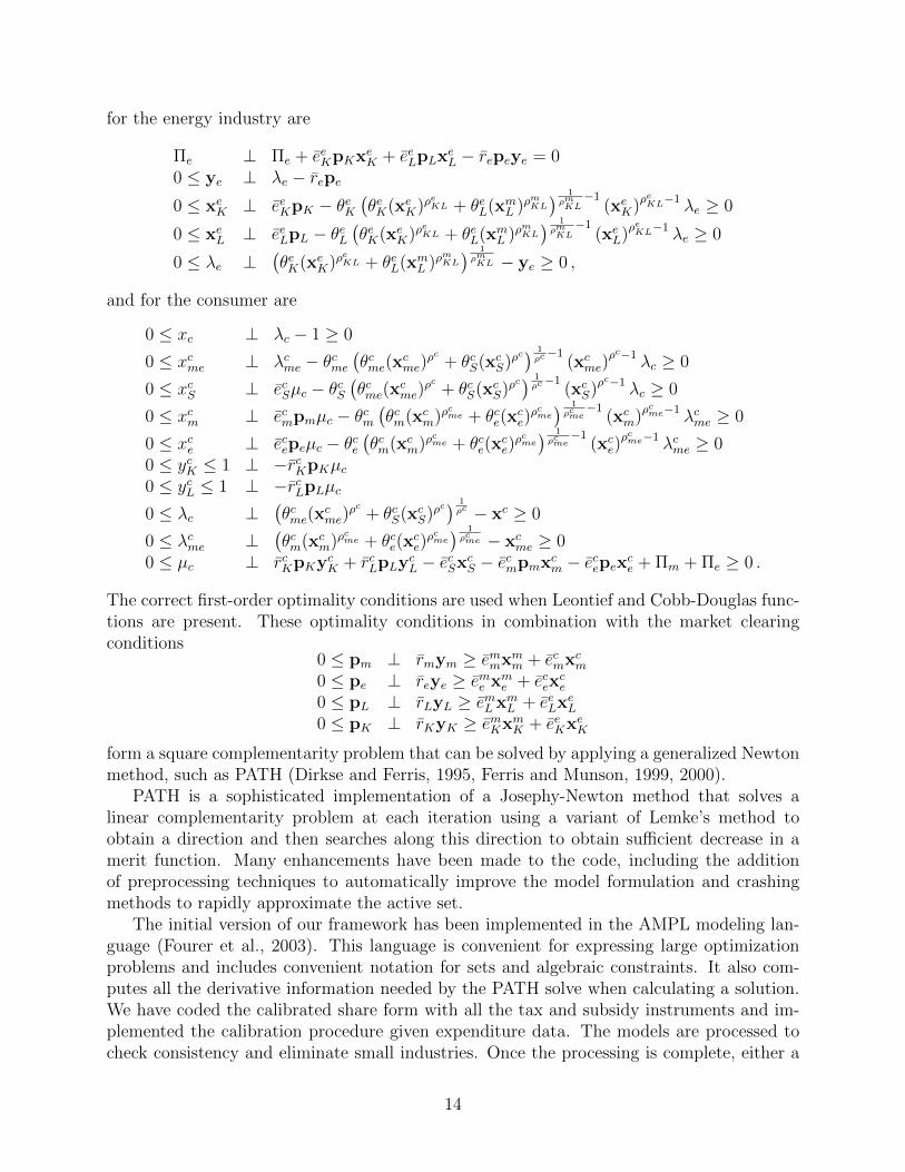
The correct first-order optimality conditions are used when Leontief and Cobb-Douglas func-tions are present. These optimality conditions in combination with the market clearingconditions

0 ≤ pm ⊥ rmym ≥ emmxmm + ecmx

cm

0 ≤ pe ⊥ reye ≥ eme xme + ecex

ce

0 ≤ pL ⊥ rLyL ≥ emL xmL + eeLx

eL

0 ≤ pK ⊥ rKyK ≥ emKxmK + eeKx

eK

form a square complementarity problem that can be solved by applying a generalized Newtonmethod, such as PATH (Dirkse and Ferris, 1995, Ferris and Munson, 1999, 2000).

PATH is a sophisticated implementation of a Josephy-Newton method that solves alinear complementarity problem at each iteration using a variant of Lemke’s method toobtain a direction and then searches along this direction to obtain sufficient decrease in amerit function. Many enhancements have been made to the code, including the additionof preprocessing techniques to automatically improve the model formulation and crashingmethods to rapidly approximate the active set.

The initial version of our framework has been implemented in the AMPL modeling lan-guage (Fourer et al., 2003). This language is convenient for expressing large optimizationproblems and includes convenient notation for sets and algebraic constraints. It also com-putes all the derivative information needed by the PATH solve when calculating a solution.We have coded the calibrated share form with all the tax and subsidy instruments and im-plemented the calibration procedure given expenditure data. The models are processed tocheck consistency and eliminate small industries. Once the processing is complete, either a

14

scalar AMPL model can be emitted and checked by the user, or the model can be solved byapplying the PATH algorithm. The construction of the first-order optimality conditions forthe industry and consumer problems is completely automated. Summary reports are writtento user-defined files.

4 Dynamic Stochastic Models

In this section, we describe optimal growth problems that illustrate the economic elements ofdynamic stochastic general equilibrium models. We then outline the computational strategieswe use to solve them.

4.1 Optimal Growth Problems

The simplest optimal growth model is the deterministic, discrete-time infinite-horizon opti-mal growth model, which solves the problem:

V (k0) =

maxc,l,k

∞∑t=0

βtu(ct, lt)

s.t. kt+1 = F (kt, lt)− ct ∀t ≥ 0 ,

where kt is the capital stock at time t with k0 given; lt is the labor supply; ct is the consump-tion; F (k, l) = k + f(k, l), where f(k, l) is the aggregate net production function; u(ct, lt) isthe utility function; and β is the discount factor.

In the comparable stochastic optimal growth model, we let θ denote the current produc-tivity level and f(k, l, θ) denote net output. Define F (k, l, θ) = k + f(k, l, θ), and assumeθ follows the stochastic law θt+1 = g(θt, εt), where εt are i.i.d. disturbances. Then theinfinite-horizon discrete-time optimization problem becomes

V (k0, θ0) =

maxc,l,k

E

{∞∑t=0

βtu(ct, lt)

}s.t. kt+1 = F (kt, lt, θt)− ct + εt ∀t ≥ 0

θt+1 = g(θt, εt) ∀t ≥ 0 ,

where k0 and θ0 are given and E{. . . } is the expectation conditional on current information,θ represents the productivity level, and εt and εt are independent i.i.d. disturbances. Bothmodels model can be extended to include heterogeneous types of capital and labor.

A generic, infinite-horizon, optimal decision-making problem has the following generalform:

V (x0) = maxat∈D(xt)

E

{∞∑t=0

βtu(xt, at)

},

where xt is the state process with initial state x0, D(xt) is the set of possible actions, at isthe action taken, and β is the discount factor.

15

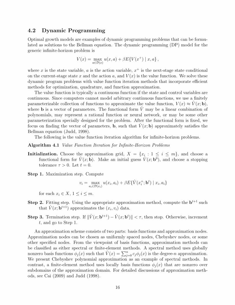
4.2 Dynamic Programming

Optimal growth models are examples of dynamic programming problems that can be formu-lated as solutions to the Bellman equation. The dynamic programming (DP) model for thegeneric infinite-horizon problem is

V (x) = maxa∈D(x)

u(x, a) + βE{V (x+) | x, a} ,

where x is the state variable, a is the action variable, x+ is the next-stage state conditionalon the current-stage state x and the action a, and V (x) is the value function. We solve thesedynamic program problems with value function iteration methods that incorporate efficientmethods for optimization, quadrature, and function approximation.

The value function is typically a continuous function if the state and control variables arecontinuous. Since computers cannot model arbitrary continuous functions, we use a finitelyparameterizable collection of functions to approximate the value function, V (x) ≈ V (x;b),where b is a vector of parameters. The functional form V may be a linear combination ofpolynomials, may represent a rational function or neural network, or may be some otherparameterization specially designed for the problem. After the functional form is fixed, wefocus on finding the vector of parameters, b, such that V (x;b) approximately satisfies theBellman equation (Judd, 1998).

The following is the value function iteration algorithm for infinite-horizon problems.

Algorithm 4.1 Value Function Iteration for Infinite-Horizon Problems

Initialization. Choose the approximation grid, X = {xi : 1 ≤ i ≤ m}, and choose afunctional form for V (x;b). Make an initial guess V (x;b0), and choose a stoppingtolerance τ > 0. Let t = 0.

Step 1. Maximization step. Compute

vi = maxai∈D(xi)

u(xi, ai) + βE{V (x+i ;bt) | xi, ai}

for each xi ∈ X, 1 ≤ i ≤ m.

Step 2. Fitting step. Using the appropriate approximation method, compute the bt+1 suchthat V (x;bt+1) approximates the (xi, vi) data.

Step 3. Termination step. If ‖V (x;bt+1)− V (x;bt)‖ < τ , then stop. Otherwise, incrementt, and go to Step 1.

An approximation scheme consists of two parts: basis functions and approximation nodes.Approximation nodes can be chosen as uniformly spaced nodes, Chebyshev nodes, or someother specified nodes. From the viewpoint of basis functions, approximation methods canbe classified as either spectral or finite-element methods. A spectral method uses globallynonzero basis functions φj(x) such that V (x) =

∑nj=0 cjφj(x) is the degree-n approximation.

We present Chebyshev polynomial approximation as an example of spectral methods. Incontrast, a finite-element method uses locally basis functions φj(x) that are nonzero oversubdomains of the approximation domain. For detailed discussions of approximation meth-ods, see Cai (2009) and Judd (1998).

16

Chebyshev Polynomial Approximation Chebyshev polynomials on [−1, 1] are definedas Tj(x) = cos(j cos−1(x)), while general Chebyshev polynomials on [a, b] are defined asTj(

2x−a−bb−a

)for j = 0, 1, 2, . . .. These polynomials are orthogonal under the weighted inner

product:

〈f, g〉 =

∫ b

a

f(x)g(x)w(x)dx

with the weighting function

w(x) =

(1−

(2x− a− bb− a

)2)−1/2

.

We approximate V with the least-squares polynomial approximation with respect to theweighting function, that is, a degree-n polynomial Vn(x), such that

Vn(x) ∈ arg mindeg(V )≤n

∫ b

a

(V (x)− Vn(x)

)2

w(x)dx .

The least-squares degree-n polynomial approximation Vn(x) on [−1, 1] has the form

Vn(x) =1

2c0 +

n∑j=1

cjTj(x),

where

cj =2

π

∫ 1

−1

V (x)Tj(x)√1− x2

dx ∀ j = 0, 1, . . . , n

are the Chebyshev least-squares coefficients.

Multidimensional Tensor Chebyshev Approximation In a d-dimensional approxi-mation problem, let a = (a1, . . . , ad) and b = (b1, . . . , bd) with bi > ai for i = 1, . . . , d.Let x = (x1, . . . , xd) with xi ∈ [ai, bi] for i = 1, . . . , d. For simplicity, we denote this set asx ∈ [a, b]. Let α = (α1, . . . , αd) be a vector of nonnegative integers. Let Tα(z) denote the ten-sor product Tα1(z1) · · ·Tαd(zd) for z = (z1, . . . , zd) ∈ [−1, 1]d. Let (2x−a− b)./(b−a) denote

the vector(

2x1−a1−b1b1−a1 , . . . , 2xd−ad−bd

bd−ad

). Then the degree-n tensor Chebyshev approximation

for V (x) is

Vn(x) =∑

0≤αi≤n,1≤i≤d

cαTα ((2x− a− b)./(b− a)) .

Multidimensional Complete Chebyshev Approximation Tensor product approxi-mations are expensive to use. Instead we use the degree-n complete Chebyshev approxima-tion for V (x), which is

Vn(x) =∑

0≤|α|≤n

cαTα ((2x− a− b)./(b− a)) ,

17

where |α| denotes∑d

i=1 αi for the nonnegative integer vector α = (α1, . . . , αd). We know the

number of terms with 0 ≤ |α| =∑d

i=1 αi ≤ n is(n+dd

)for the degree-n complete Chebyshev

approximation in Rd, while the number of terms for the tensor Chebyshev approximation is(n + 1)d. The complexity of computation of a degree-n complete Chebyshev polynomial ismuch less than the complexity of computing a tensor Chebyshev polynomial in Rd.

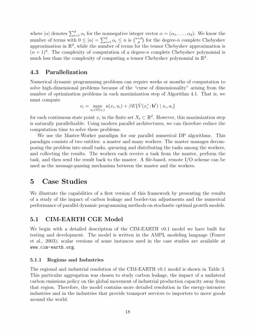
4.3 Parallelization

Numerical dynamic programming problems can require weeks or months of computation tosolve high-dimensional problems because of the “curse of dimensionality” arising from thenumber of optimization problems in each maximization step of Algorithm 4.1. That is, wemust compute

vi = maxai∈D(xi)

u(xi, ai) + βE{V (x+i ;bt) | xi, ai}

for each continuous state point xi in the finite set Xt ⊂ Rd. However, this maximization stepis naturally parallelizable. Using modern parallel architectures, we can therefore reduce thecomputation time to solve these problems.

We use the Master-Worker paradigm for our parallel numerical DP algorithms. Thisparadigm consists of two entities: a master and many workers. The master manages decom-posing the problem into small tasks, queueing and distributing the tasks among the workers,and collecting the results. The workers each receive a task from the master, perform thetask, and then send the result back to the master. A file-based, remote I/O scheme can beused as the message-passing mechanism between the master and the workers.

5 Case Studies

We illustrate the capabilities of a first version of this framework by presenting the resultsof a study of the impact of carbon leakage and border-tax adjustments and the numericalperformance of parallel dynamic programming methods on stochastic optimal growth models.

5.1 CIM-EARTH CGE Model

We begin with a detailed description of the CIM-EARTH v0.1 model we have built fortesting and development. The model is written in the AMPL modeling language (Foureret al., 2003); scalar versions of some instances used in the case studies are available atwww.cim-earth.org.

5.1.1 Regions and Industries

The regional and industrial resolution of the CIM-EARTH v0.1 model is shown in Table 3.This particular aggregation was chosen to study carbon leakage, the impact of a unilateralcarbon emissions policy on the global movement of industrial production capacity away fromthat region. Therefore, the model contains more detailed resolution in the energy-intensiveindustries and in the industries that provide transport services to importers to move goodsaround the world.

18

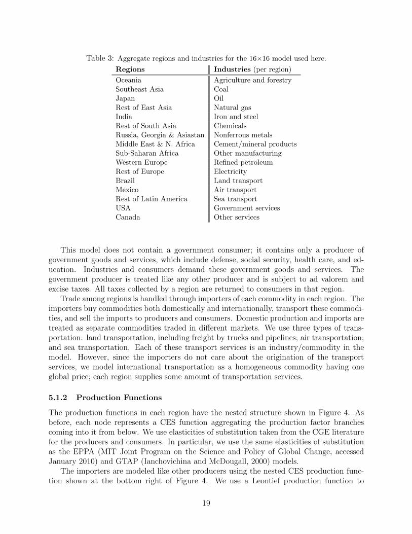
Table 3: Aggregate regions and industries for the 16×16 model used here.

Regions Industries (per region)

Oceania Agriculture and forestrySoutheast Asia CoalJapan OilRest of East Asia Natural gasIndia Iron and steelRest of South Asia ChemicalsRussia, Georgia & Asiastan Nonferrous metalsMiddle East & N. Africa Cement/mineral productsSub-Saharan Africa Other manufacturingWestern Europe Refined petroleumRest of Europe ElectricityBrazil Land transportMexico Air transportRest of Latin America Sea transportUSA Government servicesCanada Other services

This model does not contain a government consumer; it contains only a producer ofgovernment goods and services, which include defense, social security, health care, and ed-ucation. Industries and consumers demand these government goods and services. Thegovernment producer is treated like any other producer and is subject to ad valorem andexcise taxes. All taxes collected by a region are returned to consumers in that region.

Trade among regions is handled through importers of each commodity in each region. Theimporters buy commodities both domestically and internationally, transport these commodi-ties, and sell the imports to producers and consumers. Domestic production and imports aretreated as separate commodities traded in different markets. We use three types of trans-portation: land transportation, including freight by trucks and pipelines; air transportation;and sea transportation. Each of these transport services is an industry/commodity in themodel. However, since the importers do not care about the origination of the transportservices, we model international transportation as a homogeneous commodity having oneglobal price; each region supplies some amount of transportation services.

5.1.2 Production Functions

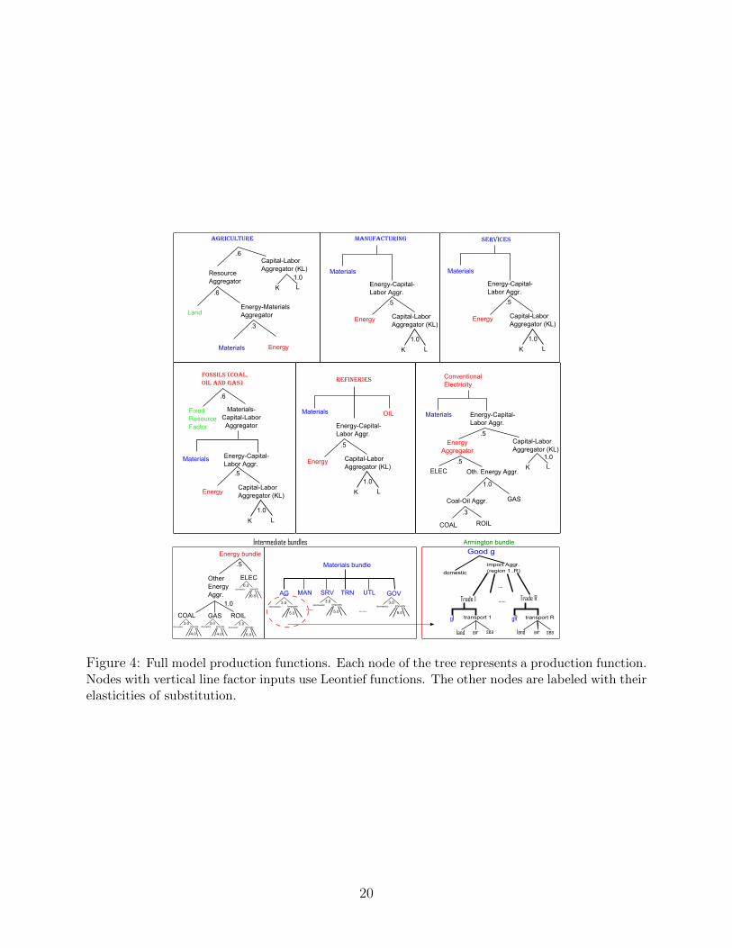
The production functions in each region have the nested structure shown in Figure 4. Asbefore, each node represents a CES function aggregating the production factor branchescoming into it from below. We use elasticities of substitution taken from the CGE literaturefor the producers and consumers. In particular, we use the same elasticities of substitutionas the EPPA (MIT Joint Program on the Science and Policy of Global Change, accessedJanuary 2010) and GTAP (Ianchovichina and McDougall, 2000) models.

The importers are modeled like other producers using the nested CES production func-tion shown at the bottom right of Figure 4. We use a Leontief production function to

19

AGRICULTURE

ResourceAggregator

Energy-MaterialsAggregatorLand

Capital-LaborAggregator (KL)

K L

1.0

.6

.6

.3

EnergyMaterials

SERVICES

Energy-Capital-Labor Aggr.


K L

1.0

.5

Energy

Materials

MANUFACTURING



K L

1.0

.5

Energy

Materials

Energy bundle

ELECOtherEnergyAggr.

COAL GAS ROIL

.5

1.0

domestic imports domestic imports domestic imports

domestic imports

3.0 3.0 3.0

0.3

4.0 4.0 6.0

0.5

Each node of a tree represents a CES type production function with the given substiution elasticity. Nodes with vertical line factor inputs use zero elasticity CES functions (Liontief type functions).



K L

1.0

EnergyAggregator

ELEC Oth. Energy Aggr.

.5

.5

GAS

COAL ROIL

Coal-Oil Aggr.

1.0

.3

OIL



K L

1.0

.5

Energy

FOSSILS (COAL, OIL AND GAS)

FixedResourceFactor

.6

Materials-Capital-LaborAggregator

Materials



K L

Energy

1.0

.5

domestic imports3.0

5.0

Materials bundle

AG MAN SRV TRN UTL GOV

domestic imports3.0

5.0

domestic imports3.0

5.0...... .......

Intermediate bundles

Materials Materials

Armington bundle

domestic

import Aggr. (region 1..R)

Trade 1 Trade R......

....

Good g

g1 transport 1

land air sea

gR transport R

land air sea

Figure 4: Full model production functions. Each node of the tree represents a production function.Nodes with vertical line factor inputs use Leontief functions. The other nodes are labeled with theirelasticities of substitution.

20

aggregate between the imported good and the relevant total transport margin so that theamount of transport demanded scales with the amount of the good imported. We use asubnest to represent the importer use of air, land, and sea transport with a small elasticityof substitution, σ = 0.2.

We use the GTAP database for the base-year revenues and expenditures. In particular,our share parameters are calibrated with the GTAP v7 database of global expenditure valuesfor 2004 (Gopalakrishnan and Walmsley, 2008). Emission amounts are obtained from theenergy volume information in GTAP-E (Burniaux and Truong, 2002).

5.1.3 Dynamic Trajectories

We solve a myopic general equilibrium model with dynamic trajectories for the factor endow-ments and efficiency units. Thus far we have prototyped exogenous statistical trend forecastsfor labor endowment, labor productivity, energy efficiency, agricultural land endowment, landproductivity (yield), and fossil resource availability and extraction technology. These simpledynamics provide a stable basis for model testing. We now describe several examples ofthese dynamic trajectories in more detail.

Capital Accumulation We use a perfectly fluid model of capital with a 4% yearly depre-ciation rate. Investment contributes to consumer utility, with investment amounts calibratedto historical data. Investment enters the consumer utility function in a Cobb-Douglas nestwith the government services and consumption bundles, implying that a fixed share of con-sumer income in each year goes to government services, investment, and consumption. Inparticular, the consumer buys the output from an industry that produces capital goods. Thisindustry behaves as any other, demanding material goods and services in order to producethe capital good. This industry, however, does not demand capital, labor, or energy. By farthe largest expenditure of the capital goods industry is on construction services, reflectingthe fact that most capital is buildings, with sizable demands from other industries, such asmachinery, transport equipment, and computing equipment.

The capital endowment in the next period is obtained from the dynamic equation

ycK,t+1 = (1− δ)ycK,t +xcI,0ycK,0

xI,t

where the capital depreciation rate, δ, is exogenously specified and the ratio in the equationis available from data, with the boundary condition ycK,0 = 1.

Labor Productivity Another primary economic driver is population growth and increasedlabor productivity. We use population data from 1950 to 2008, with forecasts to 2050, fromthe 2008 United Nations population database (U.N. Population Division). Historical eco-nomic activity rates, the fraction of people that participate in the economy either with a jobor looking for a job, from 1980 to 2006 are taken from the International Labor Organization(International Labor Organization Department of Statistics), along with projections to 2020.We combine these projections to estimate the labor endowments in each region.

Increasing productivity is modeled by inclusion of a productivity factor γL multiplyingthe labor endowment in the consumer problem, where γL(t) is the labor productivity in

21

Reserves =

1.6101 T bbl

1900 1950 2000 2050 21000

1

2

3

4

Oil

extr

acti

onHG

tonn

es�yr

L

Reserves =

371137. km3

1980 2000 2020 2040 2060 2080 21001.0

1.5

2.0

2.5

3.0

3.5

4.0

4.5

Gas

extr

acti

onH'0

00km

3 �yrL

Reserves =

1411.28 Gtonnes

1980 2000 2020 2040 2060 2080 21004

6

8

10

Coa

lext

ract

ion

HGto

nnes

�yrL

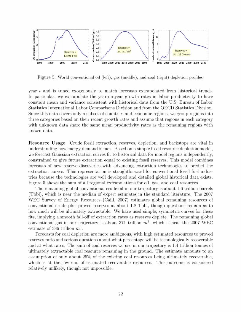
Figure 5: World conventional oil (left), gas (middle), and coal (right) depletion profiles.

year t and is tuned exogenously to match forecasts extrapolated from historical trends.In particular, we extrapolate the year-on-year growth rates in labor productivity to haveconstant mean and variance consistent with historical data from the U.S. Bureau of LaborStatistics International Labor Comparisons Division and from the OECD Statistics Division.Since this data covers only a subset of countries and economic regions, we group regions intothree categories based on their recent growth rates and assume that regions in each categorywith unknown data share the same mean productivity rates as the remaining regions withknown data.

Resource Usage Crude fossil extraction, reserves, depletion, and backstops are vital inunderstanding how energy demand is met. Based on a simple fossil resource depletion model,we forecast Gaussian extraction curves fit to historical data for model regions independently,constrained to give future extraction equal to existing fossil reserves. This model combinesforecasts of new reserve discoveries with advancing extraction technologies to predict theextraction curves. This representation is straightforward for conventional fossil fuel indus-tries because the technologies are well developed and detailed global historical data exists.Figure 5 shows the sum of all regional extrapolations for oil, gas, and coal resources.

The remaining global conventional crude oil in our trajectory is about 1.6 trillion barrels(Tbbl), which is near the median of expert estimates in the standard literature. The 2007WEC Survey of Energy Resources (Caill, 2007) estimates global remaining resources ofconventional crude plus proved reserves at about 1.8 Tbbl, though questions remain as tohow much will be ultimately extractable. We have used simple, symmetric curves for thesefits, implying a smooth fall-off of extraction rates as reserves deplete. The remaining globalconventional gas in our trajectory is about 371 trillion m3, which is near the 2007 WECestimate of 386 trillion m3.

Forecasts for coal depletion are more ambiguous, with high estimated resources to provedreserves ratio and serious questions about what percentage will be technologically recoverableand at what rates. The sum of coal reserves we use in our trajectory is 1.4 trillion tonnes ofultimately extractable coal resource remaining in the ground. The estimate amounts to anassumption of only about 25% of the existing coal resources being ultimately recoverable,which is at the low end of estimated recoverable resources. This outcome is consideredrelatively unlikely, though not impossible.

22

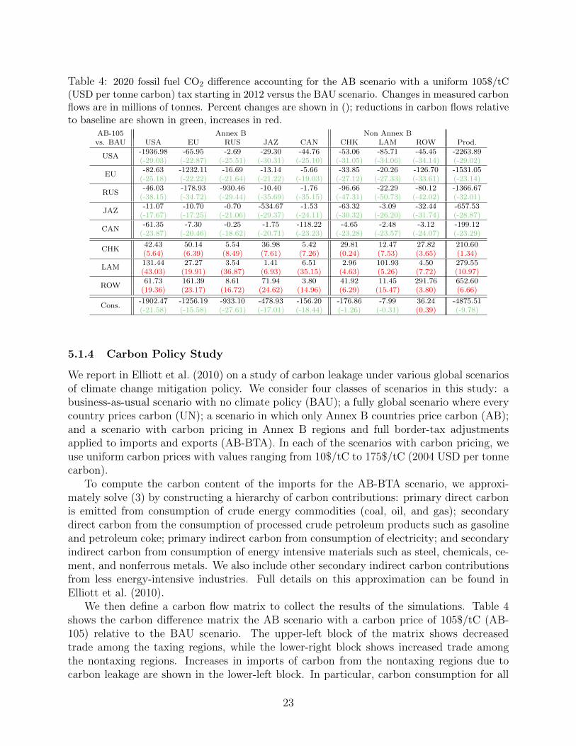
Table 4: 2020 fossil fuel CO2 difference accounting for the AB scenario with a uniform 105$/tC(USD per tonne carbon) tax starting in 2012 versus the BAU scenario. Changes in measured carbonflows are in millions of tonnes. Percent changes are shown in (); reductions in carbon flows relativeto baseline are shown in green, increases in red.

AB-105 Annex B Non Annex Bvs. BAU USA EU RUS JAZ CAN CHK LAM ROW Prod.

USA-1936.98 -65.95 -2.69 -29.30 -44.76 -53.06 -85.71 -45.45 -2263.89(-29.03) (-22.87) (-25.51) (-30.31) (-25.10) (-31.05) (-34.06) (-34.14) (-29.02)

EU-82.63 -1232.11 -16.69 -13.14 -5.66 -33.85 -20.26 -126.70 -1531.05

(-25.18) (-22.22) (-21.64) (-21.22) (-19.03) (-27.12) (-27.33) (-33.61) (-23.14)

RUS-46.03 -178.93 -930.46 -10.40 -1.76 -96.66 -22.29 -80.12 -1366.67

(-38.15) (-34.72) (-29.44) (-35.69) (-35.15) (-47.31) (-50.73) (-42.02) (-32.01)

JAZ-11.07 -10.70 -0.70 -534.67 -1.53 -63.32 -3.09 -32.44 -657.53

(-17.67) (-17.25) (-21.06) (-29.37) (-24.11) (-30.32) (-26.20) (-31.74) (-28.87)

CAN-61.35 -7.30 -0.25 -1.75 -118.22 -4.65 -2.48 -3.12 -199.12

(-23.87) (-20.46) (-18.62) (-20.71) (-23.23) (-23.28) (-23.57) (-24.07) (-23.29)

CHK42.43 50.14 5.54 36.98 5.42 29.81 12.47 27.82 210.60(5.64) (6.39) (8.49) (7.61) (7.26) (0.24) (7.53) (3.65) (1.34)

LAM131.44 27.27 3.54 1.41 6.51 2.96 101.93 4.50 279.55(43.03) (19.91) (36.87) (6.93) (35.15) (4.63) (5.26) (7.72) (10.97)

ROW61.73 161.39 8.61 71.94 3.80 41.92 11.45 291.76 652.60

(19.36) (23.17) (16.72) (24.62) (14.96) (6.29) (15.47) (3.80) (6.66)

Cons.-1902.47 -1256.19 -933.10 -478.93 -156.20 -176.86 -7.99 36.24 -4875.51(-21.58) (-15.58) (-27.61) (-17.01) (-18.44) (-1.26) (-0.31) (0.39) (-9.78)

5.1.4 Carbon Policy Study

We report in Elliott et al. (2010) on a study of carbon leakage under various global scenariosof climate change mitigation policy. We consider four classes of scenarios in this study: abusiness-as-usual scenario with no climate policy (BAU); a fully global scenario where everycountry prices carbon (UN); a scenario in which only Annex B countries price carbon (AB);and a scenario with carbon pricing in Annex B regions and full border-tax adjustmentsapplied to imports and exports (AB-BTA). In each of the scenarios with carbon pricing, weuse uniform carbon prices with values ranging from 10$/tC to 175$/tC (2004 USD per tonnecarbon).

To compute the carbon content of the imports for the AB-BTA scenario, we approxi-mately solve (3) by constructing a hierarchy of carbon contributions: primary direct carbonis emitted from consumption of crude energy commodities (coal, oil, and gas); secondarydirect carbon from the consumption of processed crude petroleum products such as gasolineand petroleum coke; primary indirect carbon from consumption of electricity; and secondaryindirect carbon from consumption of energy intensive materials such as steel, chemicals, ce-ment, and nonferrous metals. We also include other secondary indirect carbon contributionsfrom less energy-intensive industries. Full details on this approximation can be found inElliott et al. (2010).

We then define a carbon flow matrix to collect the results of the simulations. Table 4shows the carbon difference matrix the AB scenario with a carbon price of 105$/tC (AB-105) relative to the BAU scenario. The upper-left block of the matrix shows decreasedtrade among the taxing regions, while the lower-right block shows increased trade amongthe nontaxing regions. Increases in imports of carbon from the nontaxing regions due tocarbon leakage are shown in the lower-left block. In particular, carbon consumption for all

23

Figure 6: (Left) Global emissions from fossil fuel consumption for 5,000 model runs with perturbedsubstitution elasticities and (right) the relative sensitivity of global CO2 emissions. Each gray lineis a single simulated trajectory, and the black line is the mean. The dark and light blue shadedareas encompass one and two standard deviations from the mean, respectively.

taxing regions (direct and virtual) falls much more slowly than carbon production due tocarbon leakage. Depending on how the goal for an emissions target is defined, the fact canchange the necessary carbon price target by as much as 15-20%. The addition of border-taxadjustments has a small, but not insubstantial, effect.

The results of this study are uncertain due to the propagation of errors from the inputdata set, the GTAP I/O matrices, and key model parameters, the elasticities of substi-tution. Using an instance of the model having slightly different dynamic trajectories, wereport in Elliott et al. (2009b) on a study of these errors. When studying the errors dueto misspecification of the elasticity of substitution parameters, we synthesized estimates forcapital-labor substitution from several sources and simulated large portions of the relevantparameter space, focusing on parameter distributions centered on Cobb-Douglas for ease ofcomparison with other recent studies (Sokolov et al., 2009). In addition to the 16 capital-labor substitutions for each industry, we also looked at the 16 Armington trade elasticities,the 16 substitution elasticities for the import/domestic consumption decision, and 23 othersubstitutions parameters from the nested functions depicted in Figure 4, such as energy-materials substitution and the substitutability between fossil energy inputs such as coal andnatural gas. We considered symmetric Gaussian distributions with standard deviations setuniversally at 20% of mean values taken from a variety of sources (Balistreri et al., 2003,Paltsev et al., 2005, Liu et al., 2004). We performed an ensemble simulation using 5,000uncorrelated draws from the full multivariate distribution and another ensemble of 1,000draws to study a key subset, the Armington elasticities. In all the studies we explored modeloutput variables at a wide range of regional and industrial scales in order to get a full viewof the impacts of data and parameter error on forecast results. Figure 6 shows an exampleof such a sensitivity measurement for global CO2 emissions.

5.2 Parallel Stochastic Optimal Growth Problems

DPSOL is parallel dynamic programming solver being developed by Cai and Judd (Cai, 2009,Cai and Judd, 2010). This solver uses the Condor system, an open-source software frameworkfor high-throughput, distributed parallelization of computationally intensive tasks on a farm

24

of computers developed by the Condor team at the University of Wisconsin-Madison. Condoracts as a resource manager for allocating and managing the computers available in the poolof machines.

This algorithm is implemented by using the Condor Master-Worker (MW) implemen-tation. The Condor MW implementation circumvents the typical parallel programminghurdles, such as load balancing, termination detection, and distributing algorithm controlinformation to the compute nodes. Moreover, the computation in the MW system is fault-tolerant: if a worker fails in executing a portion of the computation, the master simplydistributes that portion of the computation to another worker, which can be an additionalworker available in the pool of computers. Furthermore, the user can request any numberof workers, independent of the number of tasks. If the user requests m workers and thereare n ×m tasks, then the fast computers will process more tasks than the slow machines,eliminating the load-balancing problem when n is large.

We use the multidimensional stochastic optimal growth problem to illustrate the efficiencyof the DPSOL algorithm. In particular, we solve the problem

V (k, θ) = maxc≥0,l≥0,k+,θ+

u(c, l, k+) + βE{V (k+, θ+) | k, θ, c, l}

s.t. k+ = F (k, l, θ)− ck+ ∈ [k, k] ,

where k, k+ ∈ Rd are the continuous state vectors, θ, θ+ ∈ Θ = {θj = (θj,1, . . . , θj,d) : 1 ≤j ≤ N} are discrete state vectors, c and l are the actions, β ∈ (0, 1) is the discount factor,u is the utility function, and E{·} is the expectation operator. Here k+ and θ+ are thenext-stage states dependent on the current-stage states and actions, and they are random.

We let k, θ, k+, θ+, c, and l are d-dimensional vectors with d = 10, making a DPproblem with ten continuous states and ten states taking on discrete values. We chooseβ = 0.8, [k, k] = [0.5, 3.0]d, F (k, l, θ) = k + θAkαl1−α with α = 0.25, and A = 1−β

αβ= 1, and

u(c, l, k+) =d∑i=1

[c1−γi

1− γ−B l1+η

i

1 + η

]+∑i 6=j

µij(k+i − k+

j )2,

with γ = 2, η = 1, µij = 0, and B = (1 − α)A1−γ = 0.75. Moreover, we assume θ+1 , . . . , θ

+d

are independent and the possible values of θi and θ+i are a1 = 0.9 and a2 = 1.1, and the

probability transition matrix from θi to θ+i is

P =

[0.75 0.250.25 0.75

],

for each i = 1, . . . , d. That is,

Pr[θ+ = (aj1 , . . . , ajd) | θ = (ai1 , . . . , aid)] = Pi1,j1Pi2,j2 · · ·Pid,jd ,

where Piα,jα is the (iα, jα) element of P , for any iα, jα = 1, . . . , 2 with α = 1, . . . , d. Therefore,

E{V (k+, θ+) | k, θ = (ai1 , . . . , aid), c, l}=

∑2j1,j2,...,jd=1 Pi1,j1Pi2,j2 · · ·Pid,jdV (k+

1 , . . . , k+d , aj1 , . . . , ajd) .

25

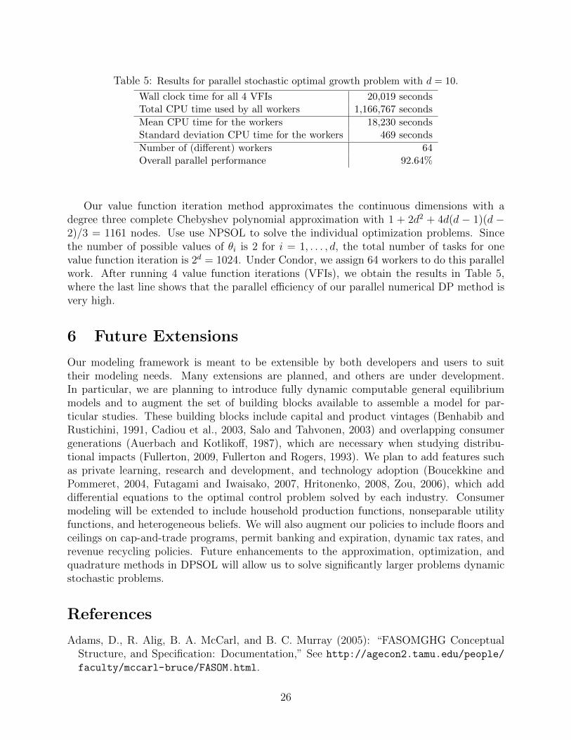
Table 5: Results for parallel stochastic optimal growth problem with d = 10.

Wall clock time for all 4 VFIs 20,019 secondsTotal CPU time used by all workers 1,166,767 seconds

Mean CPU time for the workers 18,230 secondsStandard deviation CPU time for the workers 469 seconds

Number of (different) workers 64Overall parallel performance 92.64%

Our value function iteration method approximates the continuous dimensions with adegree three complete Chebyshev polynomial approximation with 1 + 2d2 + 4d(d − 1)(d −2)/3 = 1161 nodes. Use use NPSOL to solve the individual optimization problems. Sincethe number of possible values of θi is 2 for i = 1, . . . , d, the total number of tasks for onevalue function iteration is 2d = 1024. Under Condor, we assign 64 workers to do this parallelwork. After running 4 value function iterations (VFIs), we obtain the results in Table 5,where the last line shows that the parallel efficiency of our parallel numerical DP method isvery high.

6 Future Extensions

Our modeling framework is meant to be extensible by both developers and users to suittheir modeling needs. Many extensions are planned, and others are under development.In particular, we are planning to introduce fully dynamic computable general equilibriummodels and to augment the set of building blocks available to assemble a model for par-ticular studies. These building blocks include capital and product vintages (Benhabib andRustichini, 1991, Cadiou et al., 2003, Salo and Tahvonen, 2003) and overlapping consumergenerations (Auerbach and Kotlikoff, 1987), which are necessary when studying distribu-tional impacts (Fullerton, 2009, Fullerton and Rogers, 1993). We plan to add features suchas private learning, research and development, and technology adoption (Boucekkine andPommeret, 2004, Futagami and Iwaisako, 2007, Hritonenko, 2008, Zou, 2006), which adddifferential equations to the optimal control problem solved by each industry. Consumermodeling will be extended to include household production functions, nonseparable utilityfunctions, and heterogeneous beliefs. We will also augment our policies to include floors andceilings on cap-and-trade programs, permit banking and expiration, dynamic tax rates, andrevenue recycling policies. Future enhancements to the approximation, optimization, andquadrature methods in DPSOL will allow us to solve significantly larger problems dynamicstochastic problems.

References

Adams, D., R. Alig, B. A. McCarl, and B. C. Murray (2005): “FASOMGHG ConceptualStructure, and Specification: Documentation,” See http://agecon2.tamu.edu/people/

faculty/mccarl-bruce/FASOM.html.

26

Auerbach, A. J. and L. J. Kotlikoff (1987): Dynamic Fiscal Policy, Cambridge, England:Cambridge University Press.

Balay, S., W. D. Gropp, L. C. McInnes, and B. F. Smith (1997): “Efficient management ofparallelism in object oriented numerical software libraries,” in E. Arge, A. M. Bruaset,and H. P. Langtangen, eds., Modern Software Tools in Scientific Computing, BirkhauserPress, 163–202.

Balistreri, E. J., C. A. McDaniel, and E. V. Wong (2003): “An Estimation of U.S. Industry-Level Capital-Labor Substitution,” Computational Economics 0303001, EconWPA, URLhttp://ideas.repec.org/p/wpa/wuwpco/0303001.html.

Ballard, C., D. Fullerton, J. B. Shoven, and J. Whalley (1985): A General EquilibriumModel for Tax Policy Evaluation, National Bureau of Economic Research Monograph,The University of Chicago Press.

Benhabib, J. and A. Rustichini (1991): “Vintage capital, investment, and growth,” Journalof Economic Theory, 55, 323–339.

Benson, S., L. C. McInnes, J. More, T. Munson, and J. Sarich (accessed January 2010):“Toolkit for Advanced Optimization (TAO) Web page,” See http://www.mcs.anl.gov/

tao.

Bhattacharyya, S. C. (1996): “Applied general equilibrium models for energy studies: A sur-vey,” Energy Economics, 18, 145–164, URL http://ideas.repec.org/a/eee/eneeco/

v18y1996i3p145-164.html.

Boehringer, C., T. F. Rutherford, and W. Wiegard (2003): “Computable General Equilib-rium Analysis: Opening a Black Box,” Discussion Paper 03-56, ZEW.

Boucekkine, R. and A. Pommeret (2004): “Energy saving technical progress and optimalcapital stock: The role of embodiment,” Economic Modelling, 21, 429–444.

Brooke, A., D. Kendrick, and A. Meeraus (1988): GAMS: A User’s Guide, South SanFrancisco, California: The Scientific Press.

Burniaux, J.-M. and T. Truong (2002): “GTAP-E: An Energy-Environmental Version of theGTAP Model,” GTAP Technical Papers 923, Center for Global Trade Analysis, Depart-ment of Agricultural Economics, Purdue University, URL http://ideas.repec.org/p/

gta/techpp/923.html.

Cadiou, L., S. Dees, and J.-P. Laffargue (2003): “A computational general equilibrium modelwith vintage capital,” Journal of Economic Dynamics and Control, 27, 1961–1991.

Cai, Y.-Y. (2009): Dynamic Programming and Its Applications and Economics and Finance,Ph.D. thesis, Stanford University.

Cai, Y.-Y. and K. Judd (2010): “Stable and efficient computational methods for dynamicprogramming,” Journal of the European Economic Association, 8.

27

Caill, A., ed. (2007): Survey of Energy Resources, World Energy Council.

Chesbrough, H. W. (2003): Open Innovation: The New Imperative for Creating and Profitingfrom Technology, Boston: Harvard Business School Press.

Conrad, K. (2001): “Computable General equilibrium Models in Environmental and Re-source Economics,” IVS discussion paper series 601, Institut fur Volkswirtschaft undStatistik, University of Mannheim, URL http://ideas.repec.org/p/mea/ivswpa/601.

html.

de Melo, J. (1988): “CGE Models for the Analysis of Trade Policy in Developing Countries,”Policy Research Working Paper Series 3, The World Bank, URL http://ideas.repec.

org/p/wbk/wbrwps/3.html.

Del Negro, M. and F. Schorfheide (2003): “Take your model bowling: Forecasting withgeneral equilibrium models,” Economic Review, 35–50, URL http://ideas.repec.org/

a/fip/fedaer/y2003iq4p35-50nv.88no.4.html.

Devarajan, S. and S. Robinson (2002): “The influence of computable general equilibriummodels on policy,” TMD discussion papers 98, International Food Policy Research Insti-tute (IFPRI), URL http://ideas.repec.org/p/fpr/tmddps/98.html.

Dirkse, S. P. and M. C. Ferris (1995): “The PATH solver: A non-monotone stabilizationscheme for mixed complementarity problems,” Optimization Methods and Software, 5,123–156, URL ftp://ftp.cs.wisc.edu/tech-reports/reports/1993/tr1179.ps.

Dowlatabadi, H. and M. G. Morgan (1993): “Integrated assessment of climate change,”Science, 259, 1813–1932, URL http://www.sciencemag.org.

Elliott, J., I. Foster, K. Judd, E. Moyer, and T. Munson (2009a): “CIM-EARTH: Commu-nity Integrated Model of Economic and Resource Trajectories for Humankind,” TechnicalMemorandum ANL/MCS-TM-307 Version 0.1, MCS Division, Argonne National Labora-tory.

Elliott, J., I. Foster, S. Kortum, T. Munson, F. Perez Cervantes, and D. Weisbach (2010):“Trade and Carbon Taxes,” Preprint ANL/MCS-P1709-1209, MCS Division, ArgonneNational Laboratory.

Elliott, J., M. Franklin, I. Foster, and T. Munson (2009b): “Propagation of Data Error andParametric Sensitivity in Computable General Equilibrium Model Forecasts,” PreprintANL/MCS-P1650-0709, MCS Divsion, Argonne National Laboratory.

Felten, E. (accessed January 2010): “Freedom to tinker,” See http://www.

freedom-to-tinker.com.

Ferris, M. C. and T. Munson (1999): “Interfaces to PATH 3.0: Design, implementation andusage,” Computational Optimization and Applications, 12, 207–227, URL ftp://ftp.cs.

wisc.edu/math-prog/tech-reports/97-12.ps.

28

Ferris, M. C. and T. Munson (2000): GAMS/PATH User Guide: Version 4.3, Departmentof Computer Sciences, University of Wisconsin, Madison.

Fourer, R., D. M. Gay, and B. W. Kernighan (2003): AMPL: A Modeling Language forMathematical Programming, Pacific Grove, California: Brooks/Cole–Thomson Learning,second edition.

Friedlingstein, P., P. Cox, R. Betts, L. Bopp, W. von Bloh, V. Brovkin, P. Cadule, S. Doney,M. Eby, I. Fung, G. Bala, J. John, C. Jones, F. Joos, T. Kato, M. Kawamiya, W. Knorr,K. Lindsay, H. D. Matthews, T. Raddatz, P. Rayner, C. Reick, E. Roeckner, K. G.Schnitzler, R. Schnur, K. Strassmann, A. J. Weaver, C. Yoshikawa, and N. Zeng (2006):“Climate-carbon cycle feedback analysis: Results from the C4MIP model intercompari-son,” J. Climate, 19, 3337–3353.

Fullerton, D., ed. (2009): Distributional Effects of Environmental and Energy Policy, Surrey,UK: Ashgate Publishing.

Fullerton, D. and D. L. Rogers (1993): Who Bears the Lifetime Tax Burden?, Washington,D.C.: Brookings Institution Press.

Futagami, K. and T. Iwaisako (2007): “Dynamic analysis of patent policy in an endogenousgrowth model,” Journal of Economic Theory, 132, 306–334.

Ginsburgh, V. and M. Keyzer (1997): The Structure of Applied General Equilibrium Models,Cambridge: The MIT Press.

Gopalakrishnan, B. N. and T. L. Walmsley, eds. (2008): Global Trade, Assistance, andProduction: The GTAP 7 Data Base, Purdue University: Global Trade Analysis Center,Department of Agricultural Economics.

Harrison, W. J. and K. Pearson (1994): “Computing Solutions for Large General EquilibriumModels Using GEMPACK,” Centre of Policy Studies/IMPACT Centre Working Papers ip-64, Monash University, Centre of Policy Studies/IMPACT Centre, URL http://ideas.

repec.org/p/cop/wpaper/ip-64.html.

Hritonenko, N. (2008): “Modeling of optimal investment in science and technology,” Non-linear Analysis: Hybrid Systems, 2, 220–230.

Ianchovichina, E. and R. McDougall (2000): “Theoretical Structure of Dynamic GTAP,”GTAP Technical Papers 480, Center for Global Trade Analysis, Department of Agri-cultural Economics, Purdue University, URL http://ideas.repec.org/p/gta/techpp/

480.html.

International Labor Organization Department of Statistics (accessed January 2010): Year-book of Labour Statistics Database, International Labor Organization Department of Statis-tics, see http://laborsta.ilo.org.

Johansen, L. (1960): A Multisectoral Study of Economic Growth, North Holland.

29

Judd, K. (1998): Numerical Methods in Economics, Cambridge: The MIT Press.

Kim, S., J. Edmonds, J. Lurz, S. Smith, and M. Wise (2006): “The ObjECTS Framework forIntegrated Assessment: Hybrid Modeling of Transportation,” The Energy Journal, SpecialIssue 2, 63–92.

Lee, N. (2006): “Bridging the gap between theory and practice in integrated assessment,”Environmental Impact Assessment Review, 26, 57–78, URL http://www.sciencedirect.

com/science/article/B6V9G-4G1GF34-1/2/a12585a069ae9b13717cbdf9d43ff64d.

Liu, J., C. Arndt, and T. Hertel (2004): “Parameter estimation and measures of fit in aglobal, general equilibrium model,” Journal of Economic Integration, 19, 626–649.

MIT Joint Program on the Science and Policy of Global Change (accessed January 2010):“Emissions Predictions and Policy Analysis Model,” See http://globalchange.mit.edu/igsm/eppa.html.

Paltsev, S., J. Reilly, H. Jacoby, R. Eckaus, J. McFarland, M. Sarofim, M. Asadoorian,and M. H. Babiker (2005): “The MIT Emissions Prediction and Policy Analysis (EPPA)Model: Version 4,” Technical Report 125, MIT.

Robinson, S. (1991): “Macroeconomics, financial variables, and computable general equi-librium models,” World Development, 19, 1509–1525, URL http://ideas.repec.org/a/

eee/wdevel/v19y1991i11p1509-1525.html.

Ross, M. T. (2008): “Documentation of the Applied Dynamic Analysis of the Global Econ-omy (ADAGE) Model,” Working Paper 08 01, RTI International, URL http://www.rti.

org/pubs/adage-model-doc_ross_sep08.pdf.

Rutherford, T. F. (1999): “Applied general equilibrium modeling with MPSGE as a GAMSsubsystem: An overview of the modeling framework and syntax,” Computational Eco-nomics, 14, 1–46.

Salo, S. and O. Tahvonen (2003): “On the economics of forest vintages,” Journal of EconomicDynamics and Control, 27, 1411–1435.

Scarf, H. E. and J. B. Shoven (1984): Applied General Equilibrium Analysis, Cambridge,UK: Cambridge University Press.

Scrieciu, S. S. (2007): “The inherent dangers of using computable general equilibrium modelsas a single integrated modelling framework for sustainability impact assessment: A criticalnote on Bohringer and Loschel (2006),” Ecological Economics, 60, 678–684.

Shoven, J. B. and J. Whalley (1984): “Applied general-equilibrium models of taxation andinternational trade: An introduction and survey,” Journal of Economic Literature, 22,1007–1051, URL http://ideas.repec.org/a/aea/jeclit/v22y1984i3p1007-51.html.

30

Sokolov, A. P., P. H. Stone, C. E. Forest, R. Prinn, M. C. Sarofim, M. Webster, S. Paltsev,C. A. Schlosser, D. Kicklighter, S. Dutkiewicz, J. Reilly, C. Wang, B. Felzer, J. M. Melillo,and H. D. Jacoby (2009): “Probabilistic forecast for twenty-first-century climate based onuncertainties in emissions (without policy) and climate parameters,” Journal of Climate,22, 5175–5204.

Sue Wing, I. (2004): “Computable General Equilibrium Models and Their Use in Economy-Wide Policy Analysis,” Technical Note 6, Joint Program on the Science and Policy ofGlobal Change.

U.N. Population Division (2008): World Population Prospects: The 2008 Revision Popula-tion Database, U.N. Population Division, see http://esa.un.org/unpp.

U.S. Environmental Protection Agency (2009): Economic impacts of S. 1733: The CleanEnergy Jobs and American Power Act of 2009, U.S. Environmental Protection Agency,see http://www.epa.gov/climatechange/economics/economicanalyses.html.

U.S. Environmental Protection Agency Clean Air Markets Division (2006): Documentationfor EPA Base Case 2006 (V.3.0) Using the Integrated Planning Model, U.S. EnvironmentalProtection Agency Clean Air Markets Division, see http://www.epa.gov/airmarkets/

progsregs/epa-ipm/index.html.

Vuuren, D., J. Lowe, E. Stehfest, L. Gohar, A. Hof, C. Hope, R. Warren, M. Meinshausen,and G.-K. Plattner (2009): “How well do IAMs model climate change?” IOP ConferenceSeries: Earth and Environmental Science, 6, 2005+.

Weyant, J. (2009): “A perspective on integrated assessment,” Climatic Change, 95, 317–323,URL http://dx.doi.org/10.1007/s10584-009-9612-4.

Weyant, J. P. (1999): Energy and Environmental Policy Modeling, Kluwer Academic.

Weyant, J. P. (2006): EMF 21 Multi-Greenhouse Gas Mitigation and Climate Policy, EnergyModeling Forum; The Energy Journal Special Issue.

Wilcoxen, P. J. (1988): The Effects of Environmental Regulation and Energy Prices on U.S.Economic Performance, Ph.D. thesis, Harvard University Department of Economics.

Zhao, Y., M. Wilde, and I. Foster (2007): “Virtual Data Language: A Typed WorkflowNotation for Diversely Structured Scientific Data,” in I. Taylor, E. Deelman, D. Gannon,and M. Shields, eds., Workflows for eScience, Springer, 258–278.

Zou, B. (2006): “Vintage technology, optimal investment, and technology adoption,” Eco-nomic Modeling, 23, 515–533.

The submitted manuscript has been created by the UChicago Argonne, LLC, Operator of Argonne National Laboratory (“Ar-gonne”) under Contract No. DE-AC02-06CH11357 with the U.S. Department of Energy. The U.S. Government retains foritself, and others acting on its behalf, a paid-up, nonexclusive, irrevocable worldwide license in said article to reproduce,prepare derivative works, distribute copies to the public, and perform publicly and display publicly, by or on behalf of theGovernment.

31

cim-earth: philosophy, models, and case studiestmunson/papers/cim-earth.pdf · cim-earth:...

Documents