ISSN 1403-2473 (Print) ISSN 1403-2465 (Online)

Working Paper in Economics No. 767

Compound Returns Adam Farago & Erik Hjalmarsson Department of Economics, June 2019

Compound Returns

Adam Farago and Erik Hjalmarsson∗

June 3, 2019

Abstract

We provide a theoretical basis for understanding the properties of compound re-

turns. At long horizons, multiplicative compounding induces extreme positive

skewness into individual stock returns, an effect primarily driven by single-period

volatility. As a consequence, most individual stocks perform very poorly. However,

holding just a few stocks (instead of a single one) greatly improves the long-run

prospects of an investment strategy, indicating that missing out on the “lucky few”

winner stocks is not a great concern. We show analytically how this somewhat coun-

terintuitive result arises from an interaction between compounding, diversification,

and rebalancing that has seemingly not been previously noted.

JEL classification: C58, G10.

Keywords: Compound returns; Diversification; Long-run returns; Skewness.

∗Both authors are at the Department of Economics and the Centre for Finance, University of Gothen-burg. Contact information: P.O. Box 640, SE 405 30 Gothenburg, Sweden. Email: adam.farago@cff.gu.seand erik.hjalmarsson@economics.gu.se. We have benfitted from comments by Hendrik Bessembinder,Amit Gyoal, Andrew Harvey, Oliver Linton, Lu Zhang, Filip Zikes, as well as by seminar participants atUniversity of Cambridge, City University of Hong Kong, Second Swedish National Pension Fund (AP2),and the Workshop on Financial Econometrics at Orebro University. The authors gratefully acknowledgefinancial support from Jan Wallander’s and Tom Hedelius’ Foundation and Tore Browaldh’s Foundation(grant number P19-0117) as well as from the Foundation for Economic Research in West Sweden.

1 Introduction

To a long-run investor, the total compound returns over the investment horizon is the

key quantity of interest. Despite this obvious fact, the properties of compound stock re-

turns have been left relatively unexplored in most financial research. However, as shown

in recent work by Bessembinder (2018), multiplicative compounding induces effects that

are not evident when simply looking at the properties of single-period returns. Through

simulation exercises, Bessembinder illustrates how compounding induces positive skew-

ness into multiperiod returns—even if the single-period return is symmetric—and shows

that over long horizons this skewness becomes a dominant feature of the distribution of

individual compound stock returns. The extreme skewness at long horizons results in a

majority of stocks performing very poorly, with a few exceptions that perform extremely

well. In short, compounding induces a “few-winners-take-all” effect.

In this paper, we aim to provide a firm theoretical basis for the properties of com-

pound returns. We first derive an expression for the higher order standardized moments

(including skewness) of compound returns, which can be seen as a theoretical verifica-

tion of the simulation-based findings in Bessembinder (2018). Our theoretical results

show that the effects of compounding are actually considerably more extreme than is

evident from simulations. These effects are primarily driven by the level of volatility in

the single-period return – the higher the volatility, the more extreme the effects – and are

not qualitatively affected by the specific distribution (or skewness) of the single-period

returns. In the second part of our analysis, we therefore consider the most tractable case,

where returns are log-normally distributed. In this setting, we derive some simple but

informative results on the properties of long-run compound returns. The results high-

light the key role of volatility and show that even a small amount of diversification can

tremendously improve the long-run prospects for an investment strategy. In the final part

of the analysis, we further analyze how to reconcile the clear long-run benefits of even

small degrees of diversification, with the fact that extreme skewness concentrates all the

(long-run) returns to just a small fraction of stocks and the apparent implication that

failure to own these specific stocks would lead to very poor returns.

Our study is related to the recent work by Bessembinder (2018) and also to other

recent papers that explicitly study skewness in individual stock returns (e.g., Neuberger

and Payne, 2018, and Oh and Wachter, 2018).1 Fama and French (2018) establish some

1Neuberger and Payne (2018) work with an alternative to the standard moment-based measure ofskewness, which we use here. Under their measure, the log-normal distribution has zero skew, whereaswe show here that for long horizons, log-normality can imply extreme levels of skewness in individual

1

empirical facts regarding aggregate (market-wide) compound returns. Martin (2012) an-

alyzes the pricing of long-dated claims and shows how it is determined by unlikely but

extreme discounted payoffs. His focus is on discounted returns (i.e., valuation), rather

than total payoffs, but his study also drives home the message that the expected (dis-

counted) return might be large while most realized returns are small. Arditti and Levy

(1975) seem to have been the first to note that compounding induces skewness, but their

primary focus is on portfolio choice and they do not recognize the dramatic long-run

effects of compounding that Bessembinder (2018) highlights and that we focus on in

this paper.2 In comparison to previous studies, we provide a comprehensive analysis of

the theoretical properties of (long-run) compound returns, including a full characteriza-

tion of their higher-order moments as well as an examination of the explicit effects of

compounding on returns on portfolios of stocks, with a detailed discussion of how com-

pounding interacts with diversification and portfolio rebalancing. In addition, we show

that direct empirical inference on the skewness in the compound returns of individual

stocks is essentially impossible for horizons of 10 years and longer, and theoretical re-

sults are therefore of first order importance for understanding the propeties of long-run

compound returns.

The theoretical results show that skewness in compound returns of individual stocks

will tend to grow at a pace even faster than that suggested by the (bootstrap) simulations

in Bessembinder (2018). Our results thus reinforce and sharpen the conclusions from

Bessembinder’s study and show that the effects of compounding are, by all measures,

extreme: 30-year compound returns, for a stock with a monthly volatility of 17%, have a

skewness in excess of one million. These results hold irrespective of whether the single-

period returns are symmetric or not. A (large) positive skewness in the single-period

returns does reinforce the skew-inducing effect of compounding, but the qualitative effects

of compounding are identical for symmetric single-period returns. We also analyze the

impact of mean reversion on long-run skewness, but even large degrees of mean reversion

in returns cannot affect the qualitative conclusions. The dominant factor in determining

the skewness of long-run compound returns is the volatility of the single-period returns,

and for sufficiently volatile assets, extreme skew-inducing effects from compounding seem

inevitable. In practice, this implies that long-run compound individual stock returns will

stock returns.2There is a large literature on the implications of higher moments for portfolio choice and asset

pricing. Early references, apart from Arditti and Levy (1975), include Krauss and Litzenberger (1976),Simkowitz and Beedles (1978), Scott and Horvath (1980), and Kane (1982). Examples of more recentstudies include Brunnermeier et al. (2007), Conrad et al. (2013), and Dahlquist et al. (2017).

2

tend to exhibit extreme skewness, whereas compound market returns will be considerably

less skewed. However, it should be noted that while the skewness of the market portfolio

might appear inconsequential when compared to the skewness of individual returns, the

distribution of the long-run compound market returns is still far from symmetric; for

developed markets, the skewness for aggregate 30-year compound returns would typically

be between 5 and 30.

The extreme effects of compounding renders skewness and other higher-order moments

rather meaningless as summary statistics of long-run returns. Not only is it next to

impossible to interpret and compare skewnesses of these magnitudes but, as we discuss

in detail, it is also next to impossible to estimate these moments. We instead argue that

one should focus on the quantiles of the compound returns, which can both be reliably

estimated and offer straightforward interpretations.3 Analytical calculations of quantiles

require knowledge of the entire distribution of the compound returns. For sufficiently long

horizons, one would expect compound returns to be (almost) log-normally distributed per

the central limit theorem. Empirically, we show that the log-normal approximation works

reasonably well as the implied long-run performance of various strategies (calculated

using the single-period parameter values and the log-normal distribution assumption) is

similar to the directly estimated long-run performance of these strategies. As a device for

understanding the first order properties of long-run compound returns, the log-normal

distribution therefore appears quite adequate.

Empirical results, using the CRSP sample of U.S. stocks, highlight the very strong

benefits of diversification for long-run returns. During the 30-year period from January

1987 to December 2016, the total return from a single-stock investment underperforms

the investment in one-month T-bills with 82.4% probability, and it underperforms the

equal-weighted market portfolio with 94.5% probability. However, investing in a portfolio

containing only 10 stocks during the same period provides a total return that outperforms

the T-bill investment with 93.7% probability, and investing in a portfolio of 50 stocks

brings the probability of beating the equal-weighted market portfolio close to 50%.

The extreme skewness in the individual long-run stock returns implies that just a few

3We focus on the quantiles themselves in the main text, but we also explore quantile-based measuresof skewness advocated by Kim and White (2004) in the Internet Appendix. The analysis of the quantile-based measures provides the same conclusions as those obtained from the moment-based measures,i.e., that (i) compound returns become more and more positively skewed as the horizon increases, and(ii) the dominant factor in determining the asymmetry of long-run compound returns is the single-period volatility, and higher order moments (skewness and kurtosis) of the single-period return haveonly a second order effect. To that extent, quantile-based skewness measures do not seem to add muchinformation over and above that gained from the moment-based measures.

3

stocks will end up generating most of the long-run returns. From a long-run investor

perspective, this fact seems to imply that missing out on some, or many, of these top

stocks would be devastating for portfolio performance and, absent very good stock-picking

skills, one would need to hold a portfolio with extremely many stocks to ensure against

such an outcome.4 In contrast, our results (as well as those in Bessembinder, 2018) show

that even small portfolios (e.g., holding 50 stocks out of the several thousand available)

get close to the performance of the market portfolio.5

We end with an analysis aimed at understanding how we can reconcile the clear

power of diversification for long-run investors with the extreme skewness in individual

stock returns and the few-winners-take-all empirical finding in Bessembinder (2018).6

We show that the simple intuition of viewing portfolio returns as (weighted) averages of

the constituents’ returns does not necessarily hold in a multi-period compound setting.

For the strict buy-and-hold portfolio, which never rebalances, the compound portfolio

return is indeed a weighted average of compound returns on the constituents, but if the

portfolio is periodically rebalanced, this is no longer true. The compound return on a

rebalanced portfolio can instead be viewed as the average of the compound returns on a

large number of “single-stock strategies” that can be formed from the underlying stocks.7

The number of these strategies increases exponentially with the length of the investment

horizon and can be orders of magnitude higher than the number of portfolio constituents

for long horizons, even with relatively infrequent rebalancing. Some of these single-stock

strategies are likely to have extremely large total returns—even if the constituent stocks

themselves are not among the extreme winners—which can have a considerable positive

impact on the overall return of the rebalanced portfolio.

We highlight these effects via several results in a simple theoretical setting where

4Simple combinatorics quickly reveal how large a portfolio one would need. For instance, if thereare 4, 000 stocks (approximately the current number of unique listings in the CRSP data base) and aninvestor wants an ex ante probability of 90% to hold at least 50 (75) of the 100 top performers, she wouldhave to hold a portfolio of 2, 232 (3, 186) stocks out of the 4, 000.

5It is well established in the case of single-period (monthly) returns that relatively small portfolios canattain a large fraction of the total benefits of diversification. Evans and Archer (1968) conclude that thebenefits of diversification are exhausted when a portfolio contains approximately 10 stocks. Bloomfield etal. (1977) find that around 20 stocks are needed. Statman (1987) argues that a well-diversified portfolioshould contain around 30 stocks. Campbell et al. (2001) and Campbell (2017) argue that almost 50stocks are required in recent subsamples.

6Bessembinder (2018) documents how a tiny fraction of all stocks have generated the vast majorityof wealth for investors: The top 90 U.S. stocks of all time (out of roughly 25, 000) contributed more than50 percent of all wealth accrued to investors. Just five firms generated ten percent of all wealth.

7A single-stock strategy refers to an investment strategy that holds a single stock in every period overa multiperiod investment horizon, but the actual stock held changes throughout the investment horizon(potentially every period) and is randomly selected from the available stocks.

4

the market consists of ex ante identical stocks. First, we show that the probability that

a rebalanced portfolio performs better than its best individual constituent over long-

horizons is non-zero. This is in sharp contrast to the case of the buy-and-hold portfolio,

where the return on the portfolio can never outperform its best individual component.

In a calibrated example, we find that there is a 47% probability that an equal-weighted

and monthly rebalanced portfolio of 10 stocks beats all of its constituents over a 30-year

horizon. Second, we show that relatively small portfolios can easily beat top market

performers in the long run. In the same calibration as above, there is a 97% probability

that an equal-weighted and monthly rebalanced portfolio formed by randomly choosing 50

out of 1,000 stocks outperforms the 100th best stock on the market over a 30-year horizon.

Third, we show that relatively small portfolios can have a considerable chance to beat the

market portfolio. In our setting, all stocks on the market have identical expected returns

and variances, and the equal-weighted market portfolio therefore obtains the minimum

variance. Any other portfolio can at best approach, but never exceed, a 50% probability

of beating the market. At the 30-year horizon, there is a 42% chance that the monthly

rebalanced 50-stock portfolio beats the market portfolio, despite containing only 1/20th

of all available stocks.

We view these results as highly supportive of the claim that portfolio returns are not

sensitive to missing out on the best individual performers. While the probabilities quoted

above correspond to portfolios that are rebalanced monthly, the conclusions are qualita-

tively unchanged for less frequent rebalancing; reducing the rebalancing frequency from

one month to five years (over the 30-year horizon) does not change the above numbers

considerably.

2 A motivating empirical exercise

To set the stage for our theoretical analysis, we start with some data-based summary

statistics for U.S. stock returns. For short horizons (i.e., from one month to a year), the

summary statistics can easily be obtained using monthly and annual returns of individual

stocks. However, for longer horizons (e.g., 10 or 30 years), such direct measurement

becomes more problematic since far from all stocks exist over such long periods. To get

around this issue, we follow Bessembinder (2018) and focus on returns from single-stock

strategies that randomly select one stock in each period from all the available stocks in

that period. In a bootstrap-like manner, we construct returns for a great number of

such random strategies and use these to calculate the return characteristics for different

5

holding periods. The procedure is described in detail in Appendix A, and the number of

simulated strategies is set to 200, 000. It is worth observing that while the procedure is

similar in spirit to a typical bootstrap exercise, the resulting portfolio returns represent

actual empirical returns to feasible strategies. That is, the procedure simply generates

returns for the strategy that chooses a single new random stock in each period (month),

and the temporal ordering of the underlying return data is maintained. The simulation is

implemented using monthly CRSP data on individual stock returns for the 30-year period

between January 1987 and December 2016. We restrict ourselves to a 30-year sample

period, since we will later compare the directly estimated properties of long-run (30-

year) returns, to inferred long-run properties based on short-run (1-month) parameters.

Such an exercise only makes sense if the short- and long-run quantities are based on the

same sample, as they are when the total sample is 30-year. In the main empirical analysis

presented in Section 4, results for earlier sample periods are also shown.

Table 1 shows summary statistics for returns of such single-stock strategies. The

first row corresponds to the one-month returns.8 The monthly average return is 1%,

the monthly standard deviation is 19%, and the monthly skewness is close to 4. The

remaining rows in Table 1 show summary statistics for compound returns at the 1, 5,

10, 20, and 30 year horizons. The mean and volatility increases with the horizon and,

most importantly, so does the skewness. The estimated skewness of the 5-year and 30-

year compound returns is 44 and 339, respectively. This result reiterates the message

in Bessembinder (2018), namely that the distribution of compound returns over long

horizons is highly asymmetric.

The aim of our paper is to provide a deeper understanding of the nature of this

asymmetry; its determinants and consequences. The column labeled “Impl Skew” shows

the implied skewness of compound returns calculated using the one-period moments (i.e.,

the one-month mean, variance, and skewness from the first row of the table) and an iid

assumption; the explicit formulas for calculating the implied moments of the compound

returns are derived in Section 3.1. It is immediately apparent that the implied skewness

at longer horizons is vastly greater than the directly estimated skewness. We argue in

the next section that the discrepancies between estimated and implied skewness values

in Table 1 reflect the fact that skewness is not a suitable measure to understand the

asymmetry of compound returns of individual stocks. First, as we show in Section 3.4,

8The numbers in the first row of Table 1 are close to those that one would obtain from a directcalculation of the same summary statistics using the entire pooled CRSP sample of 1-month returns.Essentially, we draw a random sample of 200,000 returns from the pooled sample and calculate thestatistics on this random sub-sample.

6

estimated skewness values for long-horizon returns (in column “Skew” of Table 1) are

severely downward biased. Second, the theoretically implied skewness values in column

“Impl Skew” are extremely high and impossible to interpret (e.g., in the order of billions

for 30-year returns).

We argue instead for focusing on the mean and quantiles of the distribution. Table 1

reports the 10th, 50th, and 90th percentiles. The 30-year mean return is 20.9, whereas

the 30-year median return is 0.12, and the 90th percentile of the 30-year returns is 7.88.

The fact that the mean is considerably higher than the 90th percentile indicates the

severe asymmetry of the distribution.

The final three columns in the table show the percent of realized strategy returns that

end up beating either the returns on the risk-free asset (the rolled over 1-month Treasury

Bill) or the market portfolio (equal- and value-weighted) over the same period. These

probabilities are strictly decreasing in the length of the holding period. If one pursues a

strategy of holding a single stock (picking a new stock every month) for a 30-year horizon,

the probability of beating the risk-free investment is only around 18%, and the probability

of beating the market is a mere 6%. This is in line with the other important message of

Bessembinder (2018): In the long-run, the typical stock (or single-stock strategy) tends

to perform much worse than the risk-free asset or the market portfolio.

In Section 4 we argue that log-normality provides a convenient and reasonably well-

working approximation to understand the above results regarding the quantiles and prob-

abilities of compound returns. Our results also reveal how diversification can vastly im-

prove upon the disappointing long-run performance of the single-stock strategy discussed

above.

3 Skewness of compound returns

3.1 Implied higher-order moments

Let x represent the one-period gross return on a given asset or portfolio. Throughout

the paper, we will denote the expected value, standard deviation, and skewness of the

one-period return as

µ ≡ E [x] , σ ≡ Std (x) =√E[(x− µ)2] , γ ≡ Skew (x) =

E[(x− µ)3]σ3

. (1)

7

Define the product process XT as

XT = x1 × x2 × ...× xT , (2)

where the xts are assumed to be independently and identically distributed (iid) and have

the same distribution as x. That is, XT represents compound returns over T periods.

Since xt is iid for all t, it is straightforward that the k-th order (non-central) moment of

XT can be calculated as

E[XkT

]= E

[xk1]× E

[xk2]× ...× E

[xkT]

= E[xk]T

. (3)

The mean and variance of XT can easily be computed using (3) as

E [XT ] = µT and V ar (XT ) =(µ2 + σ2

)T − µ2T . (4)

Proposition 1 provides a formula for the higher order standardized moments of XT .

Proposition 1 Let x and xt, t = 1, ..., T, be iid random variables, and denote

θj ≡E [xj]

E [x]j. (5)

Define the compound process XT =∏T

t=1 xt. For k > 2, the k-th order standardized

moment of the compound process is given by

E[(XT − E [XT ])k

]V ar (XT )k/2

=θTk +

(∑k−2j=1

(kj

)(−1)jθTk−j

)+ (−1)k (1− k)(

θT2 − 1)k/2 . (6)

Proof. See the proof in Appendix B.

With the help of Proposition 1, all the higher-order standardized moments of XT can

easily be obtained.9 Since we focus on the skewness of compound returns, it is useful to

spell out the formula for skewness in a separate corollary.

9Arditti and Levy (1975) derive a related result on the third moment of compound returns, althoughthey consider the non-standardized moment rather than the actual skewness. Proposition 1 generalizestheir result to all higher order (standardized) moments. Arditti and Levy (1975) note that compoundinginduces skewness, but their focus is on portfolio choice and they do not examine the long-run implicationsof compounding.

8

Corollary 1 Let x and xt, t = 1, ..., T, be iid random variables with mean µ, variance

σ2, and skewness γ. The skewness of the compound process XT =∏T

t=1 xt is

Skew (XT ) =θT3 − 3θT2 + 2(θT2 − 1

)3/2, (7)

where

θ2 =σ2

µ2+ 1 and θ3 = −2 + 3θ2 + (θ2 − 1)3/2 γ . (8)

Proof. This is a straightforward application of Proposition 1 for k = 3.

Table 2 tabulates the skewness of XT calculated via Corollary 1, when the single-

period returns correspond to monthly returns with µ = 1.01 (i.e., 1% per month) and

volatility that varies across the columns of the table. Compound returns corresponding

to 1-, 5-, 10-, 20-, and 30-year horizons are presented.

Panel A shows the skewness of compound returns, when the single-period returns

are symmetric (zero-skew). Several results are worth noting. First, compound returns

are positively skewed, and their skewness increases non-linearly with the horizon. That

is, compounding induces skewness in long-horizon returns even if single-period returns

are symmetric (as previously also noted by Arditti and Levy, 1975, and Bessembinder,

2018). Second, skewness increases dramatically and highly non-linearly in σ, for a given

T . In other words, the single-period volatility has a huge effect on the degree of skewness

induced by compounding. If the volatility of the monthly returns is σ = 0.05, which

corresponds to a well-diversified portfolio (annual volatility around 17%), then the effect

of compounding is relatively modest, although not inconsequential: The skewness of the

30-year returns is 5.19. On the other hand, for σ ≥ 0.14, which is more typical for

individual stocks, the skewness induced by compounding increases very rapidly with the

horizon. This leads to our third observation: For large T and σ, the skewness values are

extreme. For example, the skewness of 30-year returns when σ ≥ 0.17 is in the order

of millions. Arguably, it is hard to give an interpretation to any skewness level larger

than 10, and even more difficult to (intuitively) compare distributions with very large but

different skewness values. Finally, it is worth highlighting that the results in Panel A hold

for any symmetric distribution. That is, they are equally valid if one-period returns are

normally or uniformly distributed. Since the uniform distribution has a fully bounded

support, the extreme skewness in long-horizon compound returns is therefore not due

to the possibility of extremely large return realizations (i.e., it is not due to an infinite

9

support of the one-period return distribution).

The rest of Table 2 helps us understand the effect of single-period skewness. Panel B

corresponds to the case where monthly returns have a skewness equal to that of a log-

normal distribution.10 Panels C and D represent cases with more greatly skewed one-

period returns, with γ = 2 and γ = 4, respectively. Our main observation is that the

effect of single-period skewness depends on the level of the single-period volatility. When

σ is low (corresponding to well-diversified portfolios), single-period skewness does not

have a large effect on the skewness of long-horizon returns (up to a 30-year horizon).

Take the column with σ = 0.05; the skewness of the 30-year returns is 5.19 when γ = 0,

and 6.77 when γ = 4. That is, the difference in skewness at the 30-year horizon is

actually lower than at the monthly level. When single-period volatility is high, single-

period skewness can have a large effect, in absolute terms, on the skewness of compound

returns, especially at long horizons. For example, if σ = 0.17, the skewness of 30-year

returns is of the order of 106 when γ = 0, and of the order of 108 when γ = 4. However,

large absolute differences between the corresponding cells of different Panels in Table

2 only occur when the values in Panel A (where γ = 0) are already extreme. In these

cases, it is hard to give an interpretation to the differences in the extreme skewness levels.

Coming back to the example of 30-year returns when σ = 0.17, it is difficult to interpret

the difference between Skew (XT ) = 106 (Panel A) and Skew (XT ) = 108 (Panel D).

Figure 1 provides a graphical illustration of the results in Table 2 by plotting the

skewness of compound returns as a function of horizon. Single-period volatility, σ, is

varied across the panels, while differing single-period skewness, γ, is represented by dif-

ferent lines. Panel A clearly illustrates that for low single-period volatility, the skewness

in long-horizon compound returns is almost identical regardless of inherent skewness in

the single-period returns. As the volatility of the single-period returns increases (through

Panels B-D), the skewness in compound returns can easily reach extreme values. How-

ever, for a given volatility, the cases with γ = 0 and γ = 4 result in qualitatively similar

patterns. To that extent, it is the volatility of the single-period returns, and not their

skewness, which is of first order importance for the skewness of compound returns. In

other words, the patterns in Skew (XT ) are more similar within the panels of Figure 1

(where single-period skewness is varied), than they are across the panels (where single-

period volatility is varied).

10The log-normal distribution does not have an explicit skewness parameter, but its skewness is a

function of the mean and variance of the distribution. Specifically, γ = σµ

(σ2

µ2 + 3)

. As examples, for

µ = 1.01 and σ = 0.05 (0.17), the skewness is equal to 0.15 (0.51).

10

The assumption of iid single-period returns was used to derive the above results. In

the Internet Appendix, we relax the iid assumption and analyze the effects of serial de-

pendence on the skewness of compound returns. We rely on a heuristic approximation

based on the log-normal case, and arrive at a conclusion similar to the one obtained when

looking at the effect of single-period skewness. When σ is low, the effect of serial depen-

dence on long-horizon skewness is small. When σ is high, the effect of serial dependence

can be sizable, but only in the range of extreme skewness levels, where interpretation

of the different skewness values is not straightforward any more. To that extent, the

effect of serial dependence is also of second order importance compared to the effect of

single-period return volatility.

3.2 Intuition from compound binomial returns

The above analysis highlights the extreme effects of compounding on higher order mo-

ments, as long as the volatility of the single-period returns is sufficiently high. To get

some intuition behind these results, we consider a simple binomial model. Assume that

the single-period return, x, can only take two values: There is an “up-tick” in the price

with probability π that results in a gross return u, and there is a “down-tick” with prob-

ability 1−π, resulting in a gross-return d. Moreover, to isolate the effect of compounding

from that of single-period skewness, let π = 0.5, which is equivalent to assuming that the

distribution of x has zero skewness.11 The mean and standard deviation of x are then

µ =u+ d

2and σ =

u− d2

, (9)

so a given pair of mean and volatility can be matched by setting u = µ+σ and d = µ−σ.

If the xts are iid, then the total return evolves along a recombining binomial tree, and

the compound return over T periods can take on T + 1 values:

XT = uMdT−M =

(ud)M dT−2M if M ≤ T/2

(ud)T−M u2M−T if M > T/2, (10)

where M ∈ {0, 1, ..., T} denotes the number of up-ticks over the investment horizon and

T −M is the number of down-ticks. The second formulation in equation (10) reveals that

every possible value of XT can be rewritten as a product of pairs of up- and down-ticks,

11The skewness of x in the general case is γ = 1−2π√π(1−π)

, which is equal to zero only if π = 0.5.

11

ud, and some remaining up-ticks (if M > T/2) or down-ticks (if M < T/2).

The probability of experiencing M up-ticks over T periods follows a binomial dis-

tribution with parameters π and T . The first three columns of Table 3 tabulate the

probability of M or less up-ticks during a 30-year horizon, with the second column indi-

cating the value of XT in each case, using the formulation in equation (10). As is seen,

it is much more likely to observe a similar number of up- and down-ticks than it is to

observe disproportionately more moves in one direction. In other words, we are likely to

observe a relatively large number of ud pairs, which highlights the relevance of the second

formulation in equation (10). For T = 360, the maximum possible number of paired up-

and down-ticks is 180, and there is a 97% chance that we observe at least 160 ud pairs

(since P (160 ≤M ≤ 200) ≈ 0.97). Also, P (175 ≤M ≤ 185) ≈ 0.44, so there is a 44%

chance to have at least 175 ud pairs.12

The value of ud will therefore have a major impact on the behavior of long-run com-

pound returns. The fourth column of Table 3 provides actual values of XT for a given M

when µ = 1.01 and σ = 0.17, which is used to represent individual stocks. As ud = 0.991

in this case, the investment loses roughly 1% of its value after every ud pair. Since the

number of ud pairs is likely to be large, the compound effect of these losses will be highly

detrimental to the investment. There is a 72% chance that the total compound return

over the 30-year period will not exceed 11% (i.e., XT ≤ 1.11) as seen from row M = 185

of Table 3. On the other hand, since u = 1.18 is relatively large, if the number of up-ticks

happens to be disproportionately large (e.g., M ≥ 210), XT takes on extremely large

values. However, the probability of this happening is very low as P (M ≥ 210) = 0.001.

The fact that XT takes on low values with high probability and exceedingly large val-

ues with very low probability creates the extremely asymmetric distribution of long-run

compound returns that is typical in the case of individual stocks.

In the last column of Table 3, values of XT are shown when µ = 1.01 and σ = 0.05,

which is used to represent well-diversified portfolios. This parameterization implies a

completely different behavior. Since ud = 1.018, the investment gains almost 2% after

every ud pair, and the compound effect of these gains will be highly beneficial for the

total return. Consequently, there is a 99.99% chance that the total compound return

over the 30-year period will be higher than 18%, and with 68% probability the return

will exceed 1300% (as seen from rows M = 150 and M = 175 of Table 3, respectively).

On the other hand, since u = 1.06, XT does not take on such extreme values when M is

12The high probability to observe a similar number of up- and down-ticks is generally true whenπ = 0.5 and T is large.

12

large compared to the case with σ = 0.17. Altogether, these imply that the distribution

of XT is much less asymmetric when the single-period volatility is low.

The stark distinction between the volatile single stock and the well diversified portfolio

depends crucially on ud being less than one in the former case, and greater than one in

the latter case. It is straightforward to show from equation (9) that ud = µ2 − σ2. As

long as µ > 1, low single-period volatility (σ <√µ2 − 1) implies ud > 1, which leads to

similar behavior as in column 5 of Table 3, while high volatility (σ >√µ2 − 1) implies

ud < 1, leading to similar behavior as in column 4.

3.3 Skewness in the market portfolio

The above analysis highlights the extreme skewness in long-run individual stock returns.

In comparison, well diversified portfolios with low volatility, such as the market portfolio,

appear well-behaved. However, this is partly a relative statement, and in absolute terms

the long-run market returns are also quite skewed and far from symmetric. A portfolio

with a monthly volatility of σ = 0.05 (annual volatility around 17 percent), has a skewness

of about 5 in the 30-year compound returns. A monthly volatility of σ = 0.08 (annual

volatility around 28 percent) results in a skewness of over 30 at the 30-year horizon.

Empirically, the annual volatility on market indexes in developed economies typically

range from around 15 to 30 percent, depending on period and country.13 The lower

volatility (σ = 0.05) corresponds well to the U.S. market in normal times, while many

other markets exhibit higher volatility.

To illustrate how this compounding-induced skewness affects the distribution of long-

run market returns, consider the case with iid log-normally distributed 1-month returns.

In this case, the compound returns are also log-normal and their distribution is completely

pinned down by the single period mean and volatility (see detailed discussion in Section

4 below). As before, let the monthly expected returns equal µ = 1.01, in which case the

expected 30-year compound return is equal to µ360 = 35.9. If the monthly volatility is

equal to σ = 0.05 (0.08), the median 30-year compound return is equal to 23.1 (11.7), and

the 68th (77th) percentile of the 30-year distribution is equal to the mean. That is, for

σ = 0.05 (0.08), there is a 68% (77%) chance of the portfolio underperforming its 30-year

expected return. While long-run compound returns on the market portfolio, or low-

volatility portfolios in general, exhibit much lower skewness than returns on individual

13For instance, estimates based on the Dimson, Marsh, and Staunton (2002, 2014) annual returnindexes for 21 different countries suggest that annual volatility ranges between 17 and 34 percent formost market indexes, using a sample from 1950 to 2013; only one country index falls outside this interval.

13

stocks, they are still far from symmetric.

3.4 Estimating skewness

It is often of natural interest to directly estimate the properties of compound returns,

both in the strict empirical sense but also in Monte Carlo (or bootstrap) simulation

exercises. However, as we demonstrate below, in the case of individual stock returns

skewness estimates can be highly misleading because of extreme bias in the skewness

estimator in this context.

A natural estimator of skewness is

g ≡1n

∑ni=1 (zi − z)3(

1n

∑ni=1 (zi − z)2) 3

2

, (11)

where z denotes a general random variable, zi, i = 1, ..., n denotes a sample of size n, and z

is the sample average. For non-normal distributions, g is typically biased, but theoretical

expressions for the bias are generally not available (Joanes and Gill, 1998). However, a

very simple and often overlooked result implies that skewness estimates of long-horizon

compound returns from individual stocks are severely downward biased. Wilkins (1944)

shows that there is an upper limit to the absolute value of g, which depends solely on the

sample size:

|g| ≤ n− 2√n− 1

. (12)

For sample sizes of n = 20, 000 and n = 200, 000, the upper limits are 141.4 and 447.2,

respectively.14 When estimating the skewness of long-horizon compound returns from

individual stocks, these limits are highly restrictive. As discussed in Section 3.1 and

illustrated in Table 2, the skewness of long-run individual stock returns can be extreme.

If we take the example of log-normal single-period returns with a volatility of σ = 0.17,

the skewness of the 30-year compound returns is 3.6 × 106. A sample size of 1.3 × 1013

would be needed just for the upper limit in (12) not to be binding when estimating such

14Another commonly used skewness estimator is based on the unbiased central moment estimates, andcan be written as

G =

√n (n− 1)

n− 2g .

It is straightforward to see that (12) implies |G| ≤√n, which translates into essentially the same limits

as for g at sample sizes n ≥ 100. Samples sizes of n = 20, 000 or n = 200, 000 are available in the type ofbootstrap exercises that we conduct in this paper (we use n = 200, 000 draws in all cases). In a purelyempirical analysis, the sample sizes would typically be considerably smaller.

14

a high level of skewness (and the estimate would still be downward biased).

In the Internet Appendix, we show in simulation exercises that the upper limit on g

is indeed binding for feasible sample sizes. We also show that the asymptotic standard

errors on g are extremely large, even when the upper limit in equation (12) is no longer

binding. Orders of magnitudes larger sample sizes than those hinted at above would

therefore be needed to obtain skewness estimates with any meaningful precision. Direct

estimation of the moment-based measure of skewness for long-horizon compound returns

on individual stocks is therefore essentially impossible in practice.

Instead, we argue that it is more meaningful to focus on the quantiles of the dis-

tribution of the compound returns.15 Let Fz (w) = P (z ≤ w) denote the cumulative

distribution function of a general random variable z, and let qα denote the α-quantile of

this distribution, with 0 < α < 1. That is, qα is the number that solves α = Fz (qα), and

the sample quantile is given by

qα ≡ inf

{w :

1

n

n∑i=1

I {zi ≤ w} ≥ α

}. (13)

We show in the Internet Appendix that quantiles of long-horizon compound returns can

be estimated with much higher precision (compared to skewness). In particular, results

based on simulations and on the asymptotic distribution of qα both show that quantiles

can be reasonably well estimated for relevant sample sizes. Moreover, quantiles offer

straightforward interpretations, unlike the extreme values of skewness obtained for long-

horizon individual stock returns. Therefore, we strongly advocate using quantiles when

studying the distribution of long-horizon compound returns. This will be our focus in

the following section.

4 Long-horizon returns in the log-normal case

4.1 Log-normality as an approximation

Characterizing the distribution of long-run compound returns with quantiles rather than

moments is considerably more robust from an empirical perspective. However, in terms

15There exist alternative (not moment-based) measures of skewness that can be constructed from thequantiles of the distribution, and we discuss such measures in the Internet Appendix. However, ananalysis of the actual quantiles seems more informative from the perspective of learning about long-runcompound returns, as we demonstrate in Section 4.

15

of deriving theoretical properties for the compound returns, the use of quantiles is more

restrictive. The results in Section 3.1 on the (higher-order) moments of compound returns

apply to all distributions in the iid case. In contrast, theoretical calculations of quantiles

require knowledge of the full distribution of the compound returns, which is only available

in specific cases. Most prominent of these is, of course, the log-normal distribution.

As previously, let x represent the one-period gross return on a given asset or invest-

ment strategy, and let the compound return corresponding to horizon T be XT =∏T

t=1 xt,

where xt are iid for all t and have the same distribution as x. By the central limit theo-

rem, (standardized) long-run compound returns will be asymptotically (i.e., as T →∞)

log-normally distributed under very general assumptions on the distribution of x, allow-

ing for both serial dependence and heterogeneity (i.e., neither independence nor identical

distribution would be required for asymptotic log-normality to hold; see White, 2001).

For “large” T , XT should therefore be approximately log-normally distributed.

Without any specific assumptions on the distribution of x, define the following quan-

tities,

ψ ≡ log

(µ2√σ2 + µ2

)and η ≡

√log

(σ2

µ2+ 1

). (14)

Note that for typical µ and σ values corresponding to monthly stock (or portfolio) returns,

η ≈ σ. Given the iid assumption in the definition of XT , ψ and η scale up with the horizon

according to

log

E [XT ]2√V ar (XT ) + E [XT ]2

= Tψ and

√log

(V ar (XT )

E [XT ]2+ 1

)=√Tη . (15)

Further, if we assume that x is log-normally distributed, ψ and η are the parameters of

the distribution, i.e.,

E [log (x)] = ψ and Std (log (x)) = η . (16)

Coupling these observations with the implications of the central limit theorem, we have

XTApprox∼ LN

(Tψ, Tη2

). (17)

The above distributional result on compound returns is exact when x is log-normal, while

it is an approximation (via the central limit theorem) when x has a different distribution.

16

Given (17), standard results yield that the α-quantile of compound returns can be

calculated as

qα (XT ) = eTψ+√TηΦ−1(α) , (18)

where Φ−1 (·) denotes the inverse cdf of the standard normal distribution. By comparing

quantiles based on (18) with the “actual” (bootstrapped) quantiles, Panels A and B in

Figure 2 provide fairly strong support for the practical applicability of the log-normal

approximation. The lines in the graphs show the quantiles calculated via equation (18),

using the estimated mean and standard deviation of the monthly returns reported in

Table 1 (i.e., µ = 1.0102 and σ = 0.186 are used, which imply ψ = −0.0065 and η =

0.1826). The round markers in Panels A and B of Figure 2 correspond to the quantiles

estimated directly from the single-stock bootstrap exercise described in Section 2 (and

reported in Table 1), and can be thought of as representing the “actual” quantiles of the

distribution as a function of the horizon T .16 This exercise, and similar ones below, is the

main reason for focusing on a 30-year sample, where the data used to calculate the short-

run parameters exactly correspond to the data used for forming the 30-year quantiles

and other properties. We focus the discussion below on the evidence from the 1987-2016

sample, but we also provide results for the two preceding 30-year periods covering 1957-

1986 and 1927-1956, which we briefly discuss towards the end of Section 4. Overall, the

results from the different 30-year samples are qualitatively similar.

As is seen, the round markers line up quite well with the log-normal quantiles, sug-

gesting that for the distribution of the bootstrapped returns log-normality provides a

decent approximation. The correspondence between the lines and round markers is to

some extent remarkable, given that the only input to the former is the mean and volatility

of monthly returns, while the latter rely on bootstrapped 30-year returns to capture the

“actual” distribution of long-horizon compound returns.

This is not to say that we think the log-normal distribution provides a perfect char-

acterization of long-horizon stock returns, but we would argue that it seems reasonable

as a first order approximation.17 In the following subsections, we state theoretical results

16More specifically, the values of the round markers for α = 0.1, 0.5, and 0.9 in Panels A and B ofFigure 2 are taken from columns “p10”, “Median”, and “p90” of Table 1, corresponding to the quantilesof bootstrapped compound returns over 1, 5, 10, 20, and 30 years. The round markers corresponding toα = 0.25 and 0.75 are not presented in Table 1, but come from the same bootstrap exercise.

17Oh and Wachter (2018) state what is effectively the opposite conclusion: The log-normal distribu-tion implies much too extreme tail behavior at long horizons. Specifically, the extreme skewness of thedistribution of long-run compound returns suggest that most wealth (i.e., stock value) will eventually beconcentrated to just a few stocks (and in the limit only one stock). We do not disagree with their conclu-sion, but note that our results do not concern the extreme (asymptotic) tail behavior of the distribution.

17

for long-run compound returns under the log-normal approximation, and based on some

of these we further corroborate this claim.

4.2 Properties of long-run compound returns

4.2.1 Quantiles

We start with some further analysis of the quantiles under the log-normal approximation.

The median of XT corresponds to α = 0.5 in equation (18), and can thus be calculated

as Median (XT ) = eTψ. If ψ = 0, the median is one at all horizons. If ψ < 0, the

median decreases and approaches zero as the horizon increases, while ψ > 0 implies

that the median increases with the horizon. The single-stock strategy of Section 2 has

ψ = −0.0065, and correspondingly, the median of the compound return gets close to zero

as the 30-year horizon is reached (Panel A of Figure 2).

Equation (18) has important implications for the other quantiles as well. To highlight

these implications, it is useful to look at the derivative of the quantile with respect to

horizon:∂qα (XT )

∂T= qα (XT )

(ψ +

ηΦ−1 (α)

2√T

). (19)

Consider first the case when ψ < 0. All the lower quantiles (α < 0.5) are decreasing

with the horizon (since both ψ < 0 and Φ−1 (α) < 0) and they approach zero as T →∞.

Some upper quantiles may initially increase with the horizon, but for any fixed α there

is a T value where the second factor in equation (19) becomes negative, and all quantiles

will eventually decrease and approach zero as T becomes sufficiently large. This is well

illustrated in Panels A and B of Figure 2: The 75th percentile of the compound return

distribution decreases when T ≥ 90 (i.e., after 7.5 years), while the 90th percentile

decreases when T ≥ 322 (i.e., after approximately 27 years).

Turning to the ψ > 0 case, it is clear that all the upper quantiles (α ≥ 0.5) increase

with the horizon (since both ψ > 0 and Φ−1 (α) > 0). Following the same argument as in

the previous case, there are lower quantiles that initially decrease with the horizon, but

for any fixed α there is a T value, where the corresponding quantile starts to increase

and keeps on increasing as T grows further.

In practice, there are likely “real-world” restrictions on the absolute size of firms (consider, for instance,the break-ups of Standard Oil and AT&T), and some of the theoretical long-run tail implications froma simple stylized model might therefore be too extreme.

18

4.2.2 Probability of beating the risk-free investment

When trying to determine the long-run success of an asset or investment strategy, it is

natural to think about the probability that it beats a certain benchmark over a specific

horizon. One popular benchmark is the return on the risk-free asset. Let Rf denote the

one-period (monthly in our examples) gross return on the risk-free asset. Empirically,

we use the return on the 1-month T-Bill to proxy for the 1-month risk-free rate. The

total return over T periods is then RTf . It is straightforward to show that under the

log-normality assumption in (17),

P(XT ≥ RT

f

)= Φ

(√Tψ − rfη

), (20)

where rf = log (Rf ) and Φ (·) denotes the cdf of the standard normal distribution. Equa-

tion (20) provides a very clear-cut categorization. If ψ = rf , then P(XT ≥ RT

f

)= 0.5

irrespective of the horizon. If ψ > rf , the probability that the risky investment beats the

risk-free asset is always larger than 0.5, and increases with the horizon (approaching one

in the limit). If ψ < rf , the probability that the risky investment beats the risk-free asset

is always lower than 0.5, and decreases with the horizon (approaching zero in the limit).

While the value of ψ dominates the asymptotic probability of beating the risk-free rate,

the value of η still plays a role for finite T . Specifically, for ψ 6= rf , the value of η will

determine how quickly P(XT ≥ RT

f

)converges to one or zero. A smaller η implies less

variable returns, and a quicker convergence to the asymptotic probability.18

The average monthly risk-free rate during our sample period from 1987 to 2016 is

0.26%, implying rf = 0.0026, which makes ψ < rf the relevant case for the single-

stock strategy. Panel C of Figure 2 shows the probability that the compound return

from the single-stock strategy is higher than the compound risk-free rate, as a function

of the horizon. The line shows the probability calculated via equation (20), while the

round markers correspond to the “actual” probabilities based on the bootstrap exercise

of Section 2 (reported in column “%>Rf” of Table 1). The round markers line up very

well with the probabilities implied by log-normality, providing further support for the

18The formula in equation (20) implicitly assumes that the risk-free rate is constant over time. Inpractice, the risk-free rate varies across periods, and a multi-period investment that rolls over the risk-free asset each period is not risk-free to a long-run investor, in the sense that the final return realization isnot known at the time of the investment. However, in times when the 1-month risk-free rate is relativelystable, equation (20) should provide a good approximation when evaluating the risky asset against a“risk-free” benchmark. If the 1-month risk-free rate varies considerably, the formula in equation (23)likely provides a better approximation.

19

practical applicability of the log-normal approximation.

4.2.3 Probability of beating a risky benchmark

Some other typical benchmarks are risky investments themselves. As before, let x repre-

sent the single-period gross return on a given asset or investment strategy. Consider now

another risky return, xm, that represents the return on a benchmark investment. Let

% ≡log(Cov(x,xm)E[x]E[xm]

+ 1)

ηηm. (21)

For typical values corresponding to monthly stock (or portfolio) returns, % ≈ Corr (x, xm)

The compound returns on the benchmark strategy is defined as XTm =∏T

t=1 xtm. We

assume, as a natural extension to the above analysis, that (xt, xtm)′ for t = 1, ..., T are

iid and have the same joint distribution as (x, xm)′. The log-normal approximation in

the two-risky-asset case corresponds to assuming that the returns on the two strategies

are jointly log-normally distributed according to(log x

log xm

)∼ N

((ψ

ψm

),

(η2 %ηηm

%ηηm η2m

)). (22)

Standard calculations show that

P (XT ≥ XTm) = Φ

(√T

ψ − ψm√η2 + η2

m − 2%ηηm

). (23)

The probability crucially depends on the relation of the parameters ψ and ψm. If ψ = ψm,

then P (XT ≥ XTm) = 0.5 irrespective of the horizon. If ψ < ψm, the probability that

the risky investment beats the benchmark is always lower than 0.5, and decreases with

the horizon (approaching zero in the limit). If ψ > ψm, the probability that the risky

investment beats the benchmark is always larger than 0.5, and increases with the horizon

(approaching one in the limit).

Panel D of Figure 2 shows the probability of the single-stock strategy beating the

equal-weighted market portfolio, as a function of T . Similar to the other graphs in Fig-

ure 2, the line shows the probability based on the log-normal approximation (in this

case, calculated via equation (23)), while the round markers represent the “actual” prob-

abilities based on the bootstrap exercise of Section 2 (reported in column “%>EW” of

20

Table 1).19 The log-normal probabilities line up almost exactly with the bootstrapped

ones.

All the graphs in Figure 2 suggest that the log-normal distribution, at a minimum,

provides a decent approximation to the behavior of long-run compound returns, in line

with the predictions of the central limit theorem.

4.3 Long-run performance of strategies

In the previous subsections we established three simple rules that help us understand the

behavior of long-horizon compound returns, all of which are related to the parameter ψ

of the single-period return distribution. First, if ψ < 0, all quantiles of the compound

return distribution approach zero as the horizon goes to infinity, while for ψ > 0, all the

quantiles diverge as the horizon increases. Second, if ψ < rf , the probability that the

risky investment beats the risk-free asset approaches zero as the horizon goes to infinity,

while for ψ > rf , the same probability approaches one. Third, if ψ < ψm, the probability

that the risky investment (represented by ψ) beats the benchmark investment strategy

(represented by ψm) approaches zero as the horizon goes to infinity, while for ψ > ψm,

the same probability approaches one.

From the definition in equation (14), it is clear that ψ is a non-linear function of µ

and σ. Therefore, it is instructive to plot different investment strategies in the expected-

return/volatility space, together with curves corresponding to the three rules above.

Panel A of Figure 3 does so for the single-stock strategy discussed so far in the paper.

The round marker represents the single-stock strategy, with µ = 1.0102 and σ = 0.186.

The three curves represent mean/volatility combinations for which ψ = 0 (the solid line),

ψ = rf (the dashed line), and ψ = ψm (the dotted line) where the risky benchmark is

the equal-weighted market portfolio.20 Any point to the right (left) of one of these curves

indicates a mean/volatility combination with a strictly smaller (larger) value of ψ than

the value represented by the given curve. The single-stock strategy is far to the right of

all three curves, indicating ψ < 0 < rf < ψm, as discussed in Section 4.2.

Investment strategies in the upper left corner on the graphs of Figure 3 have the

greatest long-run growth prospects. This area can be approached either by increasing

19Using the value-weighted market return as the benchmark produces similar (unreported) results.20In the binomial model, discussed in Section 3.2, we showed that the return after a paired up- and

down-move is ud = µ2 − σ2. Consequently, ud = 1 defines a curve in the mean/volatility space that canbe expressed as µ =

√1 + σ2. This curve is almost identical to the ψ = 0 curve within the ranges shown

on the graphs of Figure 3. This highlights the close correspondence between the conditions ud > 1 inthe binomial model and ψ > 0 in the general case (and also between ud < 1 and ψ < 0).

21

the expected value of single-period returns (moving up) or decreasing their volatility

(moving left). One straightforward way to achieve the latter is diversification.21

Panel B of Figure 3 illustrates the effect of diversification. The panel shows the mean-

volatility characteristics of bootstrapped portfolio strategies, where the equal-weighted

portfolio of N randomly selected stocks is created every month.22 These strategies have

the same expected return (a very small variation in the actual mean is due to the bootstrap

procedure), and the increase in number of stocks thus induces a strict left-ward shift of

the round markers in the graph. The lowest variance (highest diversification) is achieved

by the equal-weighted market portfolio (represented by the diamond marker), but the

portfolio with 50 stocks is already very close. The positive effects of diversification are

clearly seen in terms of the compound returns from these strategies. Going from the

single-stock strategy to picking two stocks already ensures that the compound returns

will not eventually drop to zero (it is above the ψ = 0 curve), and including five stocks

ensures that the strategy eventually beats the risk-free rate (it is above the ψ = rf curve).

Table 4 accompanies Figure 3 and elaborates on its findings. The first two columns

give the expected return and volatility of the monthly returns for each strategy, simply

tabulating what is shown graphically in Figure 3. The next two columns show the cor-

responding ψ and η values. The remainder of the table shows the probabilities that the

30-year compound returns from the strategies beat the return on the risk-free investment

and the market portfolio (equal- or value-weighted) over the same period. The columns

labeled “actual” use the distribution of 30-year bootstrapped returns for each strategy,

while the columns labeled “implied” show the corresponding values implied by the log-

normal approximation and the single-period parameters in the first columns. Panel A

of Table 4 corresponds to the single-stock strategy, while Panels B and C present the

portfolio strategies. In general, there is a close correspondence between the values in

the “actual” and “implied” columns, and only in a few cases do the two probabilities

21Our results are meant to illustrate the statistical properties of long-run compound returns as afunction of their mean and variance, and highlight how both the mean and variance affect long-runreturns. As argued forcefully by Samuelson (1969, 1979) and Merton and Samuelson (1974), convergenceto the log-normal distribution for long-run compound returns does not imply that all investors shouldchoose the portfolio with the highest ψ.

22The same bootstrap procedure is carried out as in the case of the single-stock strategy in Section 2.The only difference is that instead of selecting a single stock in each month, multiple stocks are selectedrandomly (N ∈ {2, 5, 10, 25, 50, 100}), and the equal-weighted return of the selected stocks is calculatedfor the given month. A new portfolio is picked for each month. The universe of available stocks and thesample period is exactly the same as in Section 2. These strategies thus capture the returns on monthlyrebalanced portfolios, where the stocks are picked randomly and the portfolio is equal-weighted at thebeginning of each period.

22

differ by more than a few percentage points.23 Overall, the results in Table 4 support

the previous notion that the log-normal distribution works well as an approximation for

long-run compound returns.

Panel B of Table 4 reiterates the benefits of diversification through the example

of equal-weighted portfolios (in which case the relevant risky benchmark is the equal-

weighted market portfolio). While the probability of the single-stock strategy beating

the risk-free investment on a 30-year horizon is only 17.6%, the same probability for

portfolios containing as few as 10 stocks is 93.7%. The probability that the single-stock

strategy beats the (equal-weighted) market on a 30-year horizon is a mere 5.5%, but the

same probability for a portfolio containing only 50 stocks is 40.1%. However, it is essen-

tially impossible to push the latter probability above 50% just via (naive) diversification,

since it leaves µ unchanged and decreases σ to the level of the market at best (as shown in

Panel B of Figure 3), and hence it cannot achieve ψ > ψm. In order to achieve a probabil-

ity of beating the market in excess of 50%, one needs to find strategies that deliver higher

expected single-period returns than the market. There is an enormous literature trying

to uncover factors that help to predict cross-sectional patterns in expected single-period

returns (for recent overviews see, e.g., Harvey et al., 2016, and Kewei et al., 2019). While

the long-run implications of the results in this literature are certainly of interest, they

are outside the scope of the current paper.

Panel C of Figure 3 and Panel C of Table 4 present results for value-weighted port-

folios. In this case, the relevant risky benchmark is the value-weighted market portfolio.

The conclusions are essentially unchanged: The probability of a 10-stock portfolio beating

the risk-free investment on a 30-year horizon is 86.7%. At the same time, the probability

that a portfolio containing 50 stocks beats the (value-weighted) market over 30 years is

41.7%.

The empirical results above focus on the 30-year period from January 1987 to De-

cember 2016. Table 5 shows that the conclusions are qualitatively unchanged if previous

non-overlapping 30-year periods are considered instead (namely, January 1957 to Decem-

ber 1986 or January 1927 to December 1956).

23In some of these cases, the difference between the “actual” and “implied” probabilities differ by asomewhat substantial margin. To that extent, the results in Figure 2 might overstate the precision ofthe log-normal approximation. We stress that we do not view the log-normal distribution as a perfectrepresentation for long-run returns, but the correspondence is close enough that the use of the log-normaldistribution as a tool for understanding the main properties of long-run compound returns seems justified.

23

5 Diversification in the long run

The above analysis of compound returns highlights two conclusions (echoing those from

Bessembinder’s, 2018, simulations). First, for individual stocks the distribution of long-

run compound returns is extremely skewed, such that most stocks deliver very poor

returns while a few deliver exceptionally large returns. Second, this extreme skewness

is quickly reduced through diversification (e.g., with 50 stocks in the portfolio). Purely

mathematically, the second finding is not surprising given the results in Section 3.1, which

show that skewness-via-compounding is primarily induced by the volatility of the single-

period returns. Diversification quickly brings down the volatility and the skewness effect

is greatly diminished, resulting in a large increase in the probability that the investment

performs well in the long run.

Intuitively, however, this result is less obvious. The extreme skewness of long-horizon

individual stock returns indicates that large long-run returns are concentrated to just

a few stocks. Simple intuition might suggest that the failure to own (most of) these

stocks would severely negatively affect portfolio performance. But with long-run returns

concentrated to just a tiny fraction of firms, one would need to hold a very large number

of stocks to ensure that one does not miss out on these extreme performers. Holding

just 10 or 50 stocks should not be enough. Whereas the results in Section 3.1 provide a

“reduced form” explanation of the effects of diversification (through lowered volatility)

the subsequent analysis is intended to provide a more “structural” description of the

actual mechanics of diversification in compound portfolio returns.

5.1 Compounding, diversification, and rebalancing

Assume that there are N stocks, and let xti denote the single-period gross return on

stock i in period t. The compound return over T periods on stock i is XT i =∏T

t=1 xti. It

is fairly straightforward to show that the compound return on the “buy-and-hold” (i.e.,

the non-rebalanced) portfolio is equal to the weighted average of the constituent stocks’

compound returns, where the weights correspond to the initial portfolio. If the initial

portfolio is equal-weighted, then

XbhTp =

1

N

N∑i=1

XT i , (24)

24

where the superscript “bh” indicates that this is the buy-and-hold portfolio.24

The buy-and-hold portfolio is problematic from a diversification point of view in the

long-run. As we documented in detail before, a few of the portfolio’s constituents will

likely perform extremely well relative to the others over long horizons. Consequently, a

few stocks will dominate the buy-and-hold portfolio after long holding periods, which is

detrimental to the single-period volatility of the portfolio, i.e., it reduces the benefits of

diversification. To keep the single-period volatility of the portfolio at a low level, the

investor therefore has to rebalance occasionally.

To illustrate how compounding, diversification, and rebalancing interact, consider the

case of two stocks and an investment horizon of four periods (N = 2 and T = 4). The

compound return on the two stocks are XT1 = x11x21x31x41 and XT2 = x12x22x32x42. The

compound return on the equal-weighted buy-and-hold portfolio is

XbhTp =

1

2

2∑i=1

XT i =1

2(x11x21x31x41 + x12x22x32x42) . (25)

The compound return on the equal-weighted portfolio that is rebalanced every period is

Xr1Tp =

(x11 + x12

2

)(x21 + x22

2

)(x31 + x32

2

)(x41 + x42

2

)=

1

24(x11x21x31x41 + x11x21x31x42 + x11x21x32x41 + x11x21x32x42 +

x11x22x31x41 + x11x22x31x42 + x11x22x32x41 + x11x22x32x42 +

x12x21x31x41 + x12x21x31x42 + x12x21x32x41 + x12x21x32x42 +

x12x22x31x41 + x12x22x31x42 + x12x22x32x41 + x12x22x32x42) ,

(26)

where the “r1” superscript indicates that the portfolio is rebalanced every period. Equa-

tion (26) reveals that Xr1Tp can be interpreted as the average of the compound returns on

all possible single-stock strategies that can be formed from the underlying stocks (recall

that a single-stock strategy randomly selects one of the available stocks in each period).

Finally, to illustrate the effect of less frequent rebalancing, the return on the equal-

24Throughout Section 5, we assume that the initial portfolio is equal-weighted, and whenever thereis rebalancing, the resulting portfolio is equal-weighted again. All stocks are ex ante identical in ouranalytical framework, and therefore the equal-weighted strategy is the most natural to consider.

25

weighted portfolio that is rebalanced once after the second period is

Xr2Tp =

(x11x21 + x12x22

2

)(x31x41 + x32x42

2

)=

1

22(x11x21x31x41 + x11x21x32x42 + x12x22x31x41 + x12x22x32x42) ,

(27)

where the “r2” superscript indicates that the portfolio is rebalanced after (every) second

period. Xr2Tp can be interpreted as the average of the compound returns on a set of

single-stock strategies that are formed from the underlying stocks by combining blocks

of compound return sequences from individual stocks, where the blocks are defined as

periods between rebalancing dates.

Comparing equations (25), (26), and (27) reveals that rebalancing enables a plethora

of new strategies that are not available to the buy-and-hold investor. The buy-and-hold

investor is stuck with a combination of the compound returns accumulated from each

stock (as illustrated in equation (25)). In contrast, the investor who rebalances takes a

position in a set of single-stock strategies, combining compound return sequences for all

possible stock combinations across rebalancing blocks (as illustrated in equations (26) and

(27)). These strategies do not exist as individual stocks, but arise from the rebalancing

process. In general, the average is taken over NT/R possible strategies, where R is the

rebalancing frequency (e.g., R = 1 for the portfolio that is rebalanced after every period,

and R = T for the buy-and-hold portfolio). For long horizons, this number can easily

become extremely large. Table 6 shows the value of NT/R for different portfolio sizes

and rebalancing frequencies when the horizon is 30 years (T = 360). If there are 50

stocks in the portfolio, the compound return on the buy-and-hold portfolio is simply the

average over the 50 constituents. On the other hand, with 5-year, 1-year, and monthly

rebalancing, the compound portfolio return is the average over a huge number of single-

stock strategies of the order of 1010, 1050, and 10611, respectively.

The above discussion provides the intuition for how diversification, coupled with (at

least occasional) rebalancing, can so effectively improve the prospects for the long-run

compound returns. In a multiperiod compound setting, the portfolio return is no longer

a simple average of the constituent stocks’ returns, but rather an average of a very large

number of single-stock strategies based on the constituent stocks. Some of these single-

stock strategies are likely to have extremely large returns, even if the constituent stocks

themselves are not among the extreme winners. Provided some of these single-stock

strategies yield high enough returns, this enables the rebalanced portfolio to achieve

26

much better compound returns than a single-stock non-diversified strategy.

We now provide various results that illustrate this effect. Throughout the following

subsections we assume that all the individual stocks on the market are identical with

single-period return moments E [xti] = µ and Std (xti) = σ for all i, and the correlation

across stocks is the same with Corr (xti, xtj) = ρ for all i 6= j. Since all stocks, and thus

all stock portfolios, have identical expected returns, the effects we document arise solely

from the way the different portfolio strategies affect the shape of the distribution of the

compound returns, while keeping the mean constant. To obtain numerical results, we

always use our baseline values of µ = 1.01 and σ = 0.17.

5.2 Performance of the portfolio relative to its constituents

First, we consider the probability of the portfolio having a higher return than its con-

stituent stocks. In particular, letXT (k) denote the k-th largest element of {XT1, ..., XTN},i.e., the k-th largest total compound return over T periods from the N stocks. Conse-

quently, XT (1) is the total compound return on the best performing stock in the portfolio,

and we focus on the probability P (XTp > XT (1)). A direct implication of equation (24)

is that P(XbhTp > XT (1)

)= 0 for any portfolio size N and horizon T . That is, the total

compound return on the buy-and-hold portfolio can never be higher than the return on

its best performing constituent. The interesting question is whether the same simple in-

tuition also holds for rebalanced portfolios, e.g., whether P(Xr1Tp > XT (1)

)is also zero?

We demonstrate below that this is far from true. As far as we are aware, these results

have not been previously explored.

In Appendix C.1, we analytically derive the probability that a portfolio of two stocks

(N = 2) will outperform both its constituents at an arbitrary horizon T , when the

portfolio is rebalanced after every period (the “r1” case) and the single-period stock

returns can only take two values (the same setup as in Section 3.2). Figure 4 shows the

results for horizons up to 30 years.25 Various degrees of correlations across the stocks are

considered. There are a few important takeaways. First, P(Xr1Tp > XT (1)

)> 0 for all

T > 1, i.e., there is a non-zero probability that the portfolio has a higher total return

than any of its constituents for all horizons larger than a single period. Second, there is

25The results in Figure 4 (and later in Figure 5) are based on the binomial model where the single-period return, xti, can take only two values. However, the conclusions regarding the behavior of long-runcompound returns do not hinge on this assumption. In the Internet Appendix we provide simulationevidence that if xti is normally distributed instead (with the same mean and variance as in the binomialcase), the corresponding results are practically identical to those in Figures 4 and 5 for horizons longerthan 5 years (T > 60).

27

a general increase in P(Xr1Tp > XT (1)

)as longer investment horizons are considered. At

the 30-year horizon, there is a 74% chance that the total compound return on the portfolio

is higher than the total return on any of its constituents, if the single-period returns are

uncorrelated. Third, a positive (negative) correlation between the returns lowers (raises)

this probability, but it remains high even if the correlation is strong: There is a 58%

chance that the portfolio beats both constituents at the 30-year horizon, even with a

correlation of 0.5.

We rely on simulations to assess the effects of larger portfolio sizes and less frequent

rebalancing (see Appendix C.2 for details). Figure 5 shows the probability that the

portfolio beats its k-th best performing constituent, P (XTp > XT (k)), as a function

of k using a fixed 30-year horizon (T = 360).26 Consider first the line with the round

markers, which corresponds to the monthly rebalanced portfolio. When there are 10

stocks (Panel A), there is a 47% chance that the portfolio beats all of its constituents,

and there is a 90% chance that it beats all but one of its constituents. When the portfolio

consists of 50 stocks (Panel B), the probability that it beats all its constituents is a rather

low 4% (although still non-zero), but the probability quickly increases with k and there is

a 96% chance that the portfolio beats 45 of its 50 constituents over the 30-year horizon.

The rest of the lines in Figure 5 correspond to less frequent rebalancing. The lines

with the triangle markers show the buy-and-hold portfolio, i.e., when there is no rebal-

ancing at all during the 30-year period. As discussed previously, the probability that

the buy-and-hold portfolio beats all its constituents is zero. P(XbhTp > XT (k)

)increases

with k also in this case, but not as quickly as with monthly rebalancing. The lines with

the diamond and square markers correspond to the 1-year and 5-year rebalancing frequen-

cies, respectively. The results corresponding to yearly rebalancing (diamond) are almost

identical to those obtained for monthly rebalancing, and the results corresponding to

5-year rebalancing (square) are also very close. In other words, reducing the rebalancing

frequency from one month to five years barely changes the probabilities of the portfolio

beating its constituents. To understand the intuition behind this result, we refer back

to Table 6. For N = 50 and T = 360, the (compound) return on the buy-and-hold

portfolio is an average of the returns on the 50 constituent stocks, while the return on

the portfolio that is rebalanced once every five years is an average of the returns from

more than 1010 single-stock strategies. Going from 50 to 1010 enables enough extremely

26Single-period returns across stocks are assumed to be independent in Figure 5. We show in theInternet Appendix that, similar to Figure 4, the results are not sensitive to moderate correlations acrossstocks. The results are almost identical if we assume that the pairwise correlations between stocks is 0.1,which is close to the average correlation between monthly individual stock returns in the CRSP data.

28

well-performing single-stock strategies to be sampled, such that the overall performance

of the portfolio greatly improves. Increasing the number of single-stock strategies from

1010 to 10106 (corresponding to monthly rebalancing) brings a much smaller additional

improvement. Therefore, the performance of the portfolio that is rebalanced once every

5 years is closer to the performance of the monthly rebalanced portfolio, than to that of

the buy-and-hold portfolio.

5.3 Performance of the portfolio relative to the market

We now explicitly consider the case where the market consists of a large number of

stocks, and the portfolio contains only a small subset of all the available stocks. What

is the probability that the long-run return on the portfolio is higher than the long-run

return on the k-th best performing stock on the market? That is, we are interested in

P (XTp > X∗T (k)), where the star superscript emphasizes that X∗T (k) is the k-th best

performing stock on the market, and not only within the portfolio. Figure 6 shows the

probability that an equal-weighted and monthly rebalanced portfolio of 50 stocks beats

the k-th best from 1,000 stocks over a 30-year investment horizon in the binomial model.

The single-period returns across stocks on the market (and in the portfolio) are indepen-

dent. As is seen, the probability that a portfolio of 50 stocks has better total return than

the 60th best stock (out of 1,000) is above 50%. The probability that the portfolio beats

the 100th best stock is 97%. These results further highlight the surprisingly strong effect

of diversification on long-run compound returns. The results in Figure 6 are based on an

approximate analytical solution, with details provided in Appendix C.3. The results from

Section 5.2 suggest that moderate correlation across stocks and less frequent rebalancing

of the portfolio (down to a five-year rebalancing frequency) would not change the results

from Figure 6 considerably. We provide simulation evidence in the Internet Appendix

that confirms this intuition.

The results in this section show that portfolios can beat their constituents and even

top market performers in the long-run, illustrating how (even moderate) diversification

coupled with (occasional) rebalancing can bring dramatic changes to the properties of

long-run returns. We end with relating these findings to our previous “reduced form”

analysis in Section 4, and calculate the probability of a given portfolio beating the market.

These calculations mirror those we present in Section 4, but explicitly model the effects of

choosing a subset of stocks from the overall market. Specifically, based on equation (23),

we can derive the probability that an equal-weighted and monthly-rebalanced portfolio

29

of N stocks beats the equal-weighted and monthly-rebalanced market portfolio over the

investment horizon, T .27 Figure 7 shows the resulting probability as a function of T ,

assuming that the portfolio consists of 50 stocks chosen from a total of 1,000 stocks that

constitute the market. The probability that the portfolio beats the market decreases with

the horizon, but the decrease is slow: Even after 30 years, there is a 42% chance that the

portfolio performs better than the market. The results are not sensitive to changing the

correlation across stocks, and they even get slightly more favorable for the portfolio as

the correlation increases. Results from Section 5.2 once again suggest that less frequent

rebalancing of the portfolio would not change the probabilities from Figure 6 considerably,

and we confirm this intuition via simulations in the Internet Appendix.

In the Internet Appendix, we also show results on the probability of the 50-stock port-

folio beating the buy-and-hold market portfolio. This portfolio is defined as an initially

equal-weighed portfolio across all 1,000 stocks in the market, but with no subsequent

rebalancing. After 30 years, the portfolio weights will have deviated substantially from

the initial equal-weighting and reflect the past (compound) returns of each stock. The

buy-and-hold market portfolio can therefore be viewed as a theoretical proxy for the value-

weighted benchmark portfolio. This portfolio also represents the aggregate holdings of

the entire economy, or a representative agent of that economy, for which no rebalanc-

ing is possible. As seen in the Internet Appendix, based on simulations, the probability

that the monthly-rebalanced equal-weighted 50-stock portfolio beats the buy-and-hold

portfolio over a 30-year horizon is above 60%, reiterating and emphasizing the strong

interaction between diversification, rebalancing, and compounding.

To sum up, the results presented in this section suggest that missing out on most of

the extreme winners is not as problematic as it would initially seem. A moderate level

of diversification (e.g., having 50 stocks in the portfolio) is enough to mostly eliminate

the negative effects of the extreme skewness in long-run individual stock returns, explain-

ing the close performance of moderately diversified portfolios and the market portfolio

documented empirically in Section 4.

27The analytical formula in equation (23) is based on the log-normal approximation, so these resultsneed an explicit assumption only about the first two moments of the single-period returns, but not theirexact distribution. See Appendix D for further details.

30

6 Conclusion

We provide a theoretical analysis and characterization of the properties of compound

returns of both individual stocks and portfolios. Our key theoretical results can be

summarized as follows: (i) Compounding induces extreme skewness in the distribution

of long-run individual stock returns; (ii) The skew-inducing effect of compounding is

primarily driven by the level of single-period return volatility and diversification across

stocks quickly eliminates most (but not all) of the skewness effects of compounding, by

bringing down the volatility; (iii) Diversification, rebalancing, and compounding interact

such that compound portfolio returns can outperform the best of the underlying stocks.

The last result provides an explanation of why the concentration of large positive long-

run returns to just a few stocks (as implied by the theory and as documented empirically

by Bessembinder, 2018) does not imply that failure to hold these stocks is catastrophic

for portfolio performance, provided an otherwise diversified portfolio is held.

We also argue that higher-order moments are not a useful way of characterizing the

statistical properties of long-run compound returns. Skewness can easily be of the order of

millions for individual stock returns at a 30-year horizon and cannot be given a meaningful

interpretation. Instead, we suggest that one should study the quantiles of the distribution.

We also show that the quantiles can be reliably estimated using feasible sample sizes,

whereas skewness (and higher order moments) cannot be reliably estimated for compound

returns of individual stocks at horizons greater than 10 years. In the empirical analysis,

we highlight that the log-normal distribution provides a surprisingly accurate tool for

modelling some key properties of long-run returns.

31

Appendix

A Bootstrap exercise

We use monthly returns on all CRSP stocks from the period between January 1987 and

December 2016; the same method applies to earlier sub-samples as well. For various

investment horizons denoted by H (e.g., H = 12 for a one-year horizon), we implement

the following bootstrap procedure:

i. We randomly pick an H-month long sub-period within the full 30-year sample

denoted by month τ to month τ +H − 1. When H = 360, this always corresponds

to the full 30-year period from 1987 to 2016.

ii. At the start of month τ , we pick a stock randomly (denoted by iτ ) from all the

stocks available in CRSP for the given month. Let xτ ,iτ represent the gross return

on stock iτ in month τ .

iii. At the start of month τ + 1, we pick a new stock randomly (denoted by iτ+1). Let

xτ+1,iτ+1 represent the gross return on stock iτ+1 in month τ + 1.

iv. We repeat the procedure in (iii) for months τ + 2 to τ + H − 1. The resulting

return series{xτ ,iτ , xτ+1,iτ+1 , ..., xτ+H−1,iτ+H−1

}represents the monthly returns from

a strategy of holding a single random stock in each month over the period chosen

in (i). Let

XH =H−1∏j=0

xτ+j,iτ+j

represent the total return on this strategy.

v. We repeat (i) to (iv) a large number of times (we use 200,000 iterations) to obtain

a bootstrap distribution of the total return after H months.

32

B Proof of Proposition 1

Denoting E [x] = µ and variance V ar (x) = σ2, it is straightforward to show that

θ1 =E [x]

E [x]= 1

θ2 =E [x2]

E [x]2= 1 +

(E [x2]

E [x]2− 1

)= 1 +

(E [x2]− E [x]2

E [x]2

)= 1 +

σ2

µ2.

(A1)

To determine θk for k > 2, start with the binomial expansion of the k-th central moment,

E[(x− E [x])k

]V ar (x)k/2

=E[∑k

j=0

(kj

)(−1)jxk−jE [x]j

]V ar (x)k/2

=

∑kj=0

(kj

)(−1)jE

[xk−j

]E [x]j

V ar (x)k/2

=

(∑k−2j=0

(kj

)(−1)jE

[xk−j

]E [x]j

)+ (−1)k (1− k)E [x]k

V ar (x)k/2

=θk +

(∑k−2j=1

(kj

)(−1)jθk−j

)+ (−1)k (1− k)

(θ2 − 1)k/2.

(A2)

To get to the second line above, spell out the terms with j = k − 1 and j = k. To get

to the third line, divide both the numerator and the denominator by E [x]k, apply the

definition of θj, and separate the term with j = 0 from the sum. Rearranging equation

(A2) yields

θk = (−1)k (k − 1)−

(k−2∑j=1

(k

j

)(−1)jθk−j

)+ (θ2 − 1)k/2

E[(x− µ)k

]σk

. (A3)

Define the compound process XT = x1 × ... × xT . Since xt are iid, we have E[XjT

]=

E [xj]T

, which also implies

E[XjT

]E [XT ]j

=

(E [xj]

E [x]j

)T= θTj . (A4)

Using the binomial expansion of the k-th central moment of XT (for k > 2), the same

steps as in equation (A2), and the equality in equation (A4), we get

33

E[(XT − E [XT ])k

]V ar (XT )k/2

=E[∑k

j=0

(kj

)(−1)jXk−j

T E [XT ]j]

V ar (XT )k/2=

∑kj=0

(kj

)(−1)jE

[Xk−jT

]E [XT ]j

V ar (XT )k/2

=

(∑k−2j=0

(kj

)(−1)jE

[Xk−jT

]E [XT ]j

)+ (−1)k (1− k)E [XT ]k

V ar (XT )k/2

=θTk +

(∑k−2j=1

(kj

)(−1)jθTk−j

)+ (−1)k (1− k)(

θT2 − 1)k/2 .

(A5)

C Results for the binomial model

Suppose the random variable x represents single-period gross returns and can take two

values: u with probability π, and d with probability 1−π. Without loss of generality, let

u > d. The moments of x are

E [x] = d+π (u− d) , Std (x) =√π (1− π) (u− d)2 , Skew (x) =

1− 2π√π (1− π)

. (A6)

All the results in this Appendix are valid for a general π, but in the main text we focus

on the case where π = 0.5.

Let x and xt, t = 1, ..., T be iid random variables and define XT =∏T

t=1 xt, which

represents compound returns over T periods. XT can be written as

XT = uMdT−M , (A7)

where M is a random variable with the support {0, 1, ..., T}, representing the number

of periods when the single-period return is u. The random variable M follows a bino-

mial distribution with parameters π and T , i.e., its probability mass function (pmf) and

cumulative distribution function (cdf) are

P (M = m) = b (m;T, π) =

(T

m

)πm (1− π)T−m

P (M ≤ m) = B (m;T, π) =m∑j=0

b (j;T, π) .(A8)

Consequently, the pmf of XT is P(XT = umdT−m

)= b (m;T, π).

34

C.1 A portfolio beating its best constituent when N = 2

Assume now that there are N = 2 stocks. The joint distribution of the single-period

returns, (xt1, xt2), is described by the following table

xt1 xt2 Probability

u u πuu

u d π − πuud u π − πuud d 1− 2π + πuu

The returns on the two stocks are identically distributed and have the same distribu-

tion as before (u with probability π and d with probability 1−π). The parameter πuu de-

notes the probability that both stocks have a return u in period t. To ensure that all prob-

abilities in the above table are non-negative, we need to set max (2π − 1, 0) ≤ πuu ≤ π.

It is straightforward to show that

Corr (xt1, xt2) =(πuu − π2)

π (1− π). (A9)

The two stocks are uncorrelated (independent) only if πuu = π2.

Consider a T period setting and assume that the joint distribution of (xt1, xt2) is iid

across time for t = 1, ..., T . We introduce the following random variables:

• Luu is the number of periods where xt1 = xt2 = u,

• Lud is the number of periods where xt1 = u and xt2 = d,

• Ldu is the number of periods where xt1 = d and xt2 = u,

• Ldd is the number of periods where xt1 = xt2 = d.

Note that 0 ≤ Luu, Lud, Ldu, Ldd ≤ T and Luu + Lud + Ldu + Ldd = T . The joint

distribution of the above variables is a multinomial distribution and has the pmf

P (Luu = luu, Lud = lud, Ldu = ldu, Ldd = T − luu − lud − ldu)

=T !

luu!lud!ldu! (T − luu − lud − ldu)!πluuuu (π − πuu)lud+ldu (1− 2π + πuu)

T−luu−lud−ldu

(A10)

35

The compound return over T periods on the two stocks and on the equal-weighted port-

folio (rebalanced every period) are

XT1 = uLuu+LuddLdu+Ldd

XT2 = uLuu+LdudLud+Ldd

XTp = uLuu(u+ d

2

)Lud+Ldu

dLdd .

(A11)

For a set of values (Ldd = ldd, Lud = lud, Ldu = ldu, Luu = luu), XTp > XT1 is satisfied when

uluu(u+ d

2

)lud+ldu

dldd > uluu+luddldu+ldd ⇐⇒ (lud + ldu)log(u+d2d

)log(ud

)︸ ︷︷ ︸≡Au

> lud . (A12)

Similarly, XTp > XT2 is satisfied when

uluu(u+ d

2

)lud+ldu

dldd > uluu+ldudlud+ldd ⇐⇒ (lud + ldu)

(−

log(u+d2u

)log(ud

) )︸ ︷︷ ︸≡Ad

< lud .

(A13)

Observe that Au > Ad > 0. It can be seen from (A12) and (A13) that the portfolio

compound return is higher than both individual compound returns, i.e., XTp > XT (1) if

(lud + ldu)Au > lud > (lud + ldu)Ad . (A14)

The probability that the portfolio beats the better performing stock can be written as

P (XTp > XT (1)) =T∑l=0

P (XTp > XT (1) | Lud + Ldu = l)P (Lud + Ldu = l) . (A15)

We now derive the probabilities from the above equation. Using equation (A10), the

following probabilities can be derived (details are in the Internet Appendix)

P (Lud + Ldu = l) = b (l;T, 2 (π − πuu)) , (A16)

P (Lud = lud | Lud + Ldu = l) = b (lud; l, 0.5) , (A17)

36

where b (·; ·) represents the pmf of the binomial distribution (see equation (A8)). Com-

bining (A14) and (A17) we get

P (XTp > XT (1) | Lud + Ldu = l) = P (lAu > lud > lAd | Lud + Ldu = l)

=∑

lAu>j>lAd,j∈N

b (j; l, 0.5) . (A18)

Finally, substituting (A16) and (A18) into (A15), we arrive at

P (XTp > XT (1)) =T∑l=0

(b (l;T, 2 (π − πuu))

∑lAu>j>lAd,j∈N

b (j; l, 0.5)

). (A19)

C.2 A portfolio beating its k-th best constituent (simulation)

The results in Figure 5 are based on simulations. For a given set of (N, T,R) values, where

N is the portfolio size, T is the investment horizon, and R is the rebalancing frequency

(note that only cases where T/R is an integer number are considered) we implement the

following procedure:

i. For iteration j = 1, generate N × T iid realizations of xti (for i = 1, ..., N and

t = 1, ..., T ), where xti can take the values u or d with equal probability. Using the

simulated xti, calculate the following objects:

a. the compound return on all stocks as XT i =∏T

t=1 xti for i = 1, ..., N ,

b. the k-th largest element of {XT1, ..., XTN}, denoted as XT (k)

c. the compound return on the rebalanced portfolio (or buy-and-hold portfolio if

R = T ) as

XTp =

T/R∏τ=1

(1

N

N∑i=1

(R∏r=1

x(τ−1)T/R+r,i

)), (A20)

where x(τ−1)T/R+r,i corresponds to xti when t = (τ − 1) TR

+ r.

ii. Let Ijk = I (XTp > XT (k)), where I (·) is the indicator function. That is, Ijk

takes the value one if the portfolio compound return is larger than the k-th largest

individual compound return in iteration j.

iii. Repeat (i) to (ii) a large number of times, j = 1, ..., J (we use J = 200, 000 iter-

ations). The probability that the portfolio beats its k-th best constituent can be

estimated as P (XTp > XT (k)) = 1J

∑Jj=1 Ijk.

37

C.3 A portfolio beating the k-th best stock on the market

Assume that XT1, XT2, ..., XTN are iid random variables and let XT [k] be the k-th order

statistic, i.e., the k-th smallest value if we take a sample of XT1, XT2, ..., XTN . It is

important to note that in the main text we use XT (k) to denote the k-th largest element,

and thus

XT (k) = XT [N − k + 1] . (A21)

Consider also the iid random variables M1,M2, ...,MN , where Mi represents the number

of periods with return u corresponding to XT i, and let M [k] be the k-th order statistic

of M1,M2, ...,MN . Clearly,

XT [k] = uM [k]dT−M [k] . (A22)

The cdf of M [k] is given by

P (M [k] ≤ m) =N−k∑j=0

(N

j

)P (M > m)j P (M ≤ m)N−j (A23)

wherem ∈ {0, 1, ..., T}, andM has the distribution described in (A8). Using the notations

from (A8), we can rewrite the above as

P (M [k] ≤ m) =N−k∑j=0

(N

j

)P (M > m)j P (M ≤ m)N−j

=N−k∑j=0

(N

j

)(1−B (m;T, π))j (1− (1−B (m;T, π)))N−j

= B (N − k;N, 1−B (m;T, π)) .

(A24)

The corresponding pdf is then

P (M [k] = m) =

B (N − k;N, 1−B (0, T, π)) if m = 0

B (N − k;N, 1−B (m,T, π))−B (N − k;N, 1−B (m− 1, T, π)) if m > 0 .

(A25)

Consider now a portfolio with N stocks. It is straightforward to show that the portfolio’s

single-period mean and standard deviation are

µp = µ and σp =σ√N. (A26)

38

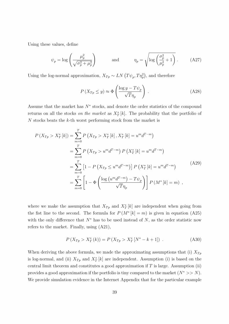
Using these values, define

ψp = log

(µ2p√

σ2p + µ2

p

)and ηp =

√log

(σ2p

µ2p

+ 1

). (A27)

Using the log-normal approximation, XTp ∼ LN(Tψp, T η

2p

), and therefore

P (XTp ≤ y) ≈ Φ

(log y − Tψp√

Tηp

). (A28)

Assume that the market has N∗ stocks, and denote the order statistics of the compound

returns on all the stocks on the market as X∗T [k]. The probability that the portfolio of

N stocks beats the k-th worst performing stock from the market is

P (XTp > X∗T [k]) =T∑

m=0

P(XTp > X∗T [k] , X∗T [k] = umdT−m

)=

T∑m=0

P(XTp > umdT−m

)P(X∗T [k] = umdT−m

)=

T∑m=0

[1− P

(XTp ≤ umdT−m

)]P(X∗T [k] = umdT−m

)=

T∑m=0

[1− Φ

(log(umdT−m

)− Tψp√

Tηp

)]P (M∗ [k] = m) ,

(A29)

where we make the assumption that XTp and X∗T [k] are independent when going from

the fist line to the second. The formula for P (M∗ [k] = m) is given in equation (A25)

with the only difference that N∗ has to be used instead of N , as the order statistic now

refers to the market. Finally, using (A21),

P (XTp > X∗T (k)) = P (XTp > X∗T [N∗ − k + 1]) . (A30)

When deriving the above formula, we made the approximating assumptions that (i) XTp

is log-normal, and (ii) XTp and X∗T [k] are independent. Assumption (i) is based on the

central limit theorem and constitutes a good approximation if T is large. Assumption (ii)

provides a good approximation if the portfolio is tiny compared to the market (N∗ >> N).

We provide simulation evidence in the Internet Appendix that for the particular example

39

showed in Figure 6 (i.e., for T = 360, N = 50, N∗ = 1000), these approximating

assumptions are fairly accurate.

D A portfolio beating the market

Assume that there are N∗ identical stocks on the market with single-period return mo-

ments E [xti] = µ and Std (xti) = σ for all i. The correlation between two stocks is

Corr (xti, xtj) = ρ for all i 6= j. Note that no further assumption (e.g., type of distri-

bution) on the single-period returns is needed. Consider a portfolio of N stocks from

the market (N ≤ N∗). Let x(N)tp denote the single-period return on the equal-weighted

portfolio of these N stocks and x(N∗)tp denote the equal-weighted market return. Since all

stocks are identical the expected return on any portfolio of these stocks is the same, i.e.,

E[x(N)tp ] = E[x

(N∗)tp ] = µ. Simple matrix algebra reveals that

Std(x

(N)tp

)=

√ρσ2 +

σ2 (1− ρ)

N, Std

(x

(N∗)tp

)=

√ρσ2 +

σ2 (1− ρ)

N∗, (A31)

and

Corr(x

(N)tp , x

(N∗)tp

)=Std

(x

(N∗)tp

)Std

(x

(N)tp

) . (A32)

These single-period return moments are used in equation (14) to get the ψ and η for the

market and the portfolio, and equation (21) is used to obtain %. Finally, the probabilities

shown in Figure 7 are obtained via the formula in equation (23).

40

References

Arditti, F., and H. Levy, 1975. Portfolio efficiency analysis in three moments: Themultiperiod case. Journal of Finance 30, 797-809.

Bessembinder, H., 2018. Do stocks outperform treasury bills? Journal of FinancialEconomics 129, 440-457.

Bloomfield, T., R. Leftwich, and J.B. Long, 1977. Portfolio Strategies and Perfor-mance. Journal of Financial Economics 5, 201-218.

Brunnermeier, M., C. Gollier, and J. Parker, 2007. Optimal beliefs, asset prices, andthe preference for skewed returns. American Economic Review 97, 159-165.

Campbell, J.Y., M. Lettau, B.G. Malkiel, and Y. Xu, 2001. Have Individual StocksBecome More Volatile? An Empirical Exploration of Idiosyncratic Risk. Journal ofFinance 56, 1-43.

Campbell, J.Y., 2017. Financial Decisions and Markets. Princeton University Press.

Conrad, J., R. Dittmar, and E. Ghysels, 2013. Ex ante skewness and expected stockreturns. Journal of Finance 68, 85-124.

Dahlquist, M., A. Farago, and R. Tedongap, 2017. Asymmetries and Portfolio Choice.The Review of Financial Studies 30, 667-702.

Dimson, E., P.R. Marsh, and M. Staunton, 2002. Triumph of the Optimists: 101Years of Global Investment Returns. Princeton University Press.

Dimson, E., P.R. Marsh, and M. Staunton, 2014. Global Investment Returns Source-book 2014. Credit Suisse/London Business School.

Evans, J.L., and S.H. Archer, 1968. Diversification and the Reduction of Dispersion:An Empirical Analysis. Journal of Finance 23, 761-767.

Fama, E., and K. French, 2018. Long horizon returns. The Review of Asset PricingStudies 8, 232–252.

Harvey, C.R., Y. Liu, and H. Zhu, 2016. ... and the Cross-Section of ExpectedReturns. The Review of Financial Studies 29, 5-68.

Joanes, D.N., and C.A. Gill, 1998. Comparing measures of sample skewness andkurtosis. Journal of the Royal Statistical Society: Series D (The Statistician), 47, 183-189.

41

Kane, A., 1982. Skewness Preference and Portfolio Choice. Journal of Financial andQuantitative Analysis 17, 15-25.

Kewei, H., C. Xue, and L. Zhang, 2019. Replicating anomalies. The Review ofFinancial Studies. Forthcoming.

Kim, T.-H., H. White, 2004. On More Robust Estimation of Skewness and Kurtosis,Finance Research Letters 1, 56-73.

Kraus, A., and R. Litzenberger, 1976. Skewness Preference and the Valuation of RiskyAssets. Journal of Finance 31 1085-1100.

Martin, I., 2012. On the Valuation of Long-Dated Assets. Journal of Political Econ-omy 120, 346-358.

Merton, R.C., and P.A. Samuleson, 1974. Fallacy of the Log-Normal Approxima-tion to Optimal Portfolio Decision-Making Over Many Periods. Journal of FinancialEconomics 1, 67-94.

Neuberger, A., and R. Payne, 2018. The Skewness of the Stock Market at LongHorizons. Working paper, Cass Business School.

Oh, S., and J.A. Wachter, 2018. Cross-sectional skewness. Working paper, TheWharton School, University of Pensylvania.

Samuelson, P.A., 1969. Lifetime Portfolio Selection by Dynamic Stochastic Program-ming. Review of Economics and Statistics 51, 239-246.

Samuelson, P.A., 1979. Why We Should Not Make Mean Log of Wealth Big ThoughYears to Act Are Long. Journal of Banking and Finance 3, 305-307.

Scott, R.C., and P.A. Horvath, 1980. On the Direction of Preference for Moments ofHigher Order than the Variance. Journal of Finance 35, 915-919.

Simkowitz, M., and W. Beedles, 1978. Diversification in a three-moment world. Jour-nal of Financial and Quantitative Analysis 13, 927-941.

Statman, M., 1987. How Many Stocks Make a Diversified Portfolio? Journal ofFinancial and Quantitative Analysis 22, 353-363.

White, H., 2001. Asymptotic Theory for Econometricians, Revised Edition. EmeraldGroup, Bingley, UK.

Wilkins, J.E., 1944. A note on skewness and kurtosis. Annals of Mathematical Statis-tics 15, 333-335.

42

Figure 1: Skewness of compound returnsThe graphs show the skewness of compound returns, Skew (XT ), as a function of the compounding

horizon, T , when single-period returns are iid. The values are calculated using equation (7). The

expected value of the single-period gross return is µ = 1.01 in all cases, the volatility of the single-period

return, σ, is varied across the panels (see above each panel), while different single-period skewness values

are represented by the different lines (see legends).

A. σ = 0.05 B. σ = 0.08

12 60 120 180 240 300 360

0

5

10

15

20

12 60 120 180 240 300 360

0

5

10

15

20

C. σ = 0.11 D. σ = 0.17

12 60 120 180 240 300 360

0

5

10

15

20

12 60 120 180 240 300 360

0

5

10

15

20

43

Figure 2: Properties of the single-stock strategyThe top two graphs show quantiles of compound returns from the single-stock strategy as a function of

the compounding horizon T . The bottom two graphs show the probability of the single-stock strategy

beating the risk-free asset (Panel C) or the equal-weighted market portfolio (Panel D) as a function of

the horizon T . In all the graphs, the lines show quantiles or probabilities calculated via the log-normal

approximation (i.e., via equation (18) in Panels A and B, equation (20) in Panel C, and equation (23)

in Panel D). For the log-normal approximation, the single-period mean and volatility of µ = 1.0102

and σ = 0.186 are used. The round markers show quantiles or probabilities estimated directly from the

single-stock bootstrap exercise in Section 2 (the corresponding values are also reported in Table 1).

A. Quantiles (10%, 25%, 50%, and 75%) B. Quantile (90%)

12 60 120 180 240 300 360

0

0.5

1

1.5

2

12 60 120 180 240 300 360

1

2

3

4

5

6

7

8

9

C. Probability of beating the risk-free asset D. Probability of beating the market

12 60 120 180 240 300 360

0

0.1

0.2

0.3

0.4

0.5

12 60 120 180 240 300 360

0

0.1

0.2

0.3

0.4

0.5

44

Figure 3: Strategies in the mean-volatility spaceThe round markers in each graph present the mean (y-axis) and volatility (x-axis) of the single-period

(monthly) gross return of different strategies. The mean and volatility values are the same as the ones

reported in columns “µ” and “σ” of Table 4 (the panels in this figure and in Table 4 correspond directly

to each other). The diamond marker in all graphs corresponds to the monthly gross return on the market

portfolio calculated using all CRSP stocks over the sample period 01/1987-12/2016; the equal-weighted

market portfolio in Panels A and B (µm = 1.0105, σm = 0.058, and ψm = 0.0088) and the value-weighted

market portfolio in Panel C (µm = 1.0090, σm = 0.045, and ψm = 0.0080). The curves represent mean-

volatility combinations for which the value of ψ, calculated via equation (14), is constant. Specifically,

they correspond to ψ = 0 (solid line), ψ = rf = 0.0026 (dashed line), and ψ = ψm (dotted line).

A. Unconditional single-stock strategy B. Portfolio strategies (equal-weighted)N=2,5,10,25,50,100 (right to left)

0 0.05 0.1 0.15 0.2 0.25

1

1.005

1.01

1.015

1.02

0 0.05 0.1 0.15 0.2 0.25

1

1.005

1.01

1.015

1.02

C. Portfolio strategies (value-weighted)N=2,5,10,25,50,100 (right to left)

0 0.05 0.1 0.15 0.2 0.25

1

1.005

1.01

1.015

1.02

45

Figure 4: Probability that a portfolio of two stocks beats its constituentsThe figure shows the probability that the total compound return on the equal-weighted and monthly

rebalanced portfolio of N = 2 stocks, XTp, is higher than the compound return on its best performing

constituent (of the two) in the binomial model. The x-axis corresponds to the investment horizon, T .

The single-period (monthly) gross return on stock i in period t can take two values, u = 1.18 or d = 0.84

with equal probability, the correlation between the two stocks is Corr(xt1, xt2) = ρ (see the legend), and

the single-period returns are iid across time. The analytical formula for obtaining the results is given in

Appendix C.1.

12 60 120 180 240 300 360

0

0.2

0.4

0.6

0.8

46

Figure 5: Probability of the portfolio beating its constituents at a 30-year horizonThe graphs show the probability that the total compound return on the equal-weighted portfolio of N

stocks, XTp, is higher than the compound return on its k-th best performing constituent, XT (k), in

the binomial model. The investment horizon is 30-years (T = 360 periods). The size of the portfolio

is varied across the graphs (see above each graph), and the various lines in each graph correspond to

different rebalancing frequencies of the portfolio (see the legends). The single-period (monthly) gross

return on stock i in period t can take two values, u = 1.18 or d = 0.84 with equal probability, and the

single-period returns are iid both across stocks and time. The results are based on simulations, with the

details provided in Appendix C.2.

A. N = 10

1 2 3 4 5 6 7 8 9 10

0

0.2

0.4

0.6

0.8

1

B. N = 50

1 3 5 7 9 11 13 15 17 19

0

0.2

0.4

0.6

0.8

1

47

Figure 6: Probability of the portfolio beating the k-th best stock on the marketThe figure shows the probability that the total compound return on the equal-weighted and monthly

rebalanced portfolio of 50 stocks, Xr1Tp, is higher than the compound return on the k-th best performing

stock, X∗T (k), out of 1,000 identical stocks in the binomial model. The x-axis corresponds to k. The

investment horizon is 30-years (T = 360 periods). The single-period (monthly) gross return on stock i in

period t can take two values, u = 1.18 or d = 0.84 with equal probability, and the single-period returns

are iid both across stocks and time. The analytical formula for calculating P(Xr1Tp > X∗

T (k))

is given

in Appendix C.3.

20 40 60 80 100 120 140

0

0.2

0.4

0.6

0.8

1

48

Figure 7: Probability of the portfolio beating the marketThe figure shows the probability that an equal weighted and monthly rebalanced portfolio of 50 stocks

beats the equal-weighted and monthly rebalanced market portfolio (consisting of 1,000 stocks) over the

investment horizon T . The single-period (monthly) gross returns, xti, have moments µ = 1.01 and

σ = 0.17 for all stocks i and periods t. Corr(xti, xtj) = ρ for all i 6= j, and different values of ρ are

considered (see the legend). The results are analytical with the details provided in Appendix D.

12 60 120 180 240 300 360

0

0.1

0.2

0.3

0.4

0.5

0.6

0.7

49

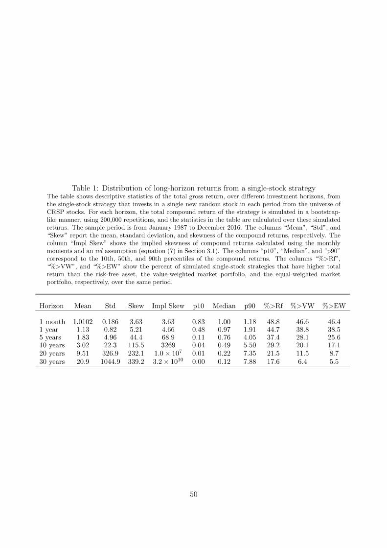
Table 1: Distribution of long-horizon returns from a single-stock strategyThe table shows descriptive statistics of the total gross return, over different investment horizons, fromthe single-stock strategy that invests in a single new random stock in each period from the universe ofCRSP stocks. For each horizon, the total compound return of the strategy is simulated in a bootstrap-like manner, using 200,000 repetitions, and the statistics in the table are calculated over these simulatedreturns. The sample period is from January 1987 to December 2016. The columns “Mean”, “Std”, and“Skew” report the mean, standard deviation, and skewness of the compound returns, respectively. Thecolumn “Impl Skew” shows the implied skewness of compound returns calculated using the monthlymoments and an iid assumption (equation (7) in Section 3.1). The columns “p10”, “Median”, and “p90”correspond to the 10th, 50th, and 90th percentiles of the compound returns. The columns “%>Rf”,“%>VW”, and “%>EW” show the percent of simulated single-stock strategies that have higher totalreturn than the risk-free asset, the value-weighted market portfolio, and the equal-weighted marketportfolio, respectively, over the same period.

Horizon Mean Std Skew Impl Skew p10 Median p90 %>Rf %>VW %>EW

1 month 1.0102 0.186 3.63 3.63 0.83 1.00 1.18 48.8 46.6 46.41 year 1.13 0.82 5.21 4.66 0.48 0.97 1.91 44.7 38.8 38.55 years 1.83 4.96 44.4 68.9 0.11 0.76 4.05 37.4 28.1 25.610 years 3.02 22.3 115.5 3269 0.04 0.49 5.50 29.2 20.1 17.120 years 9.51 326.9 232.1 1.0× 107 0.01 0.22 7.35 21.5 11.5 8.730 years 20.9 1044.9 339.2 3.2× 1010 0.00 0.12 7.88 17.6 6.4 5.5

50

Table 2: Skewness of compound returnsThe table shows the skewness of compound returns, Skew (XT ), for various compounding horizons T (indifferent rows), when single-period returns are iid. The values are calculated using equation (7). Theexpected value of the single-period gross return is µ = 1.01 in all cases, the volatility of the single-periodreturn, σ, is varied across the columns, while the skewness of the single-period return, γ, is varied acrossthe panels of the table.

T σ =0.02 σ =0.05 σ =0.08 σ =0.11 σ =0.14 σ =0.17 σ =0.20

A. γ = 01 0.00 0.00 0.00 0.00 0.00 0.00 0.0012 0.19 0.48 0.78 1.10 1.46 1.86 2.3160 0.46 1.23 2.26 3.89 6.89 13.2 28.0120 0.66 1.93 4.24 10.2 30.8 123 625240 0.97 3.36 11.7 68.5 745 1.4× 104 3.8× 105

360 1.22 5.19 32.1 513 2.0× 104 1.6× 106 2.3× 108

B. The log-normal case: γ = σµ

(σ2

µ2 + 3)

1 0.06 0.15 0.24 0.33 0.42 0.51 0.6012 0.21 0.52 0.86 1.23 1.65 2.14 2.7560 0.47 1.26 2.33 4.09 7.50 15.3 36.3120 0.67 1.95 4.35 10.8 35.1 161 1031240 0.97 3.40 12.1 75.7 960 2.3× 104 1.0× 106

360 1.23 5.25 33.54 595 2.9× 104 3.6× 106 1.0× 109

C. γ = 21 2.00 2.00 2.00 2.00 2.00 2.00 2.0012 0.77 1.09 1.46 1.88 2.39 3.03 3.8460 0.73 1.59 2.86 5.15 10.2 23.4 65.4120 0.87 2.28 5.23 14.4 57.1 351 3272240 1.13 3.85 15.3 125 2489 1.1× 105 1.0× 107

360 1.37 5.95 46.1 1260 1.2× 105 3.7× 107 3.4× 1010

D. γ = 41 4.00 4.00 4.00 4.00 4.00 4.00 4.0012 1.36 1.71 2.14 2.68 3.38 4.32 5.6160 1.00 1.95 3.50 6.61 14.5 40.4 149120 1.07 2.64 6.33 20.1 105 996 1.7× 104

240 1.29 4.36 19.8 230 8263 8.9× 105 2.7× 108

360 1.51 6.77 65.9 3083 7.3× 105 8.4× 108 4.5× 1012

51

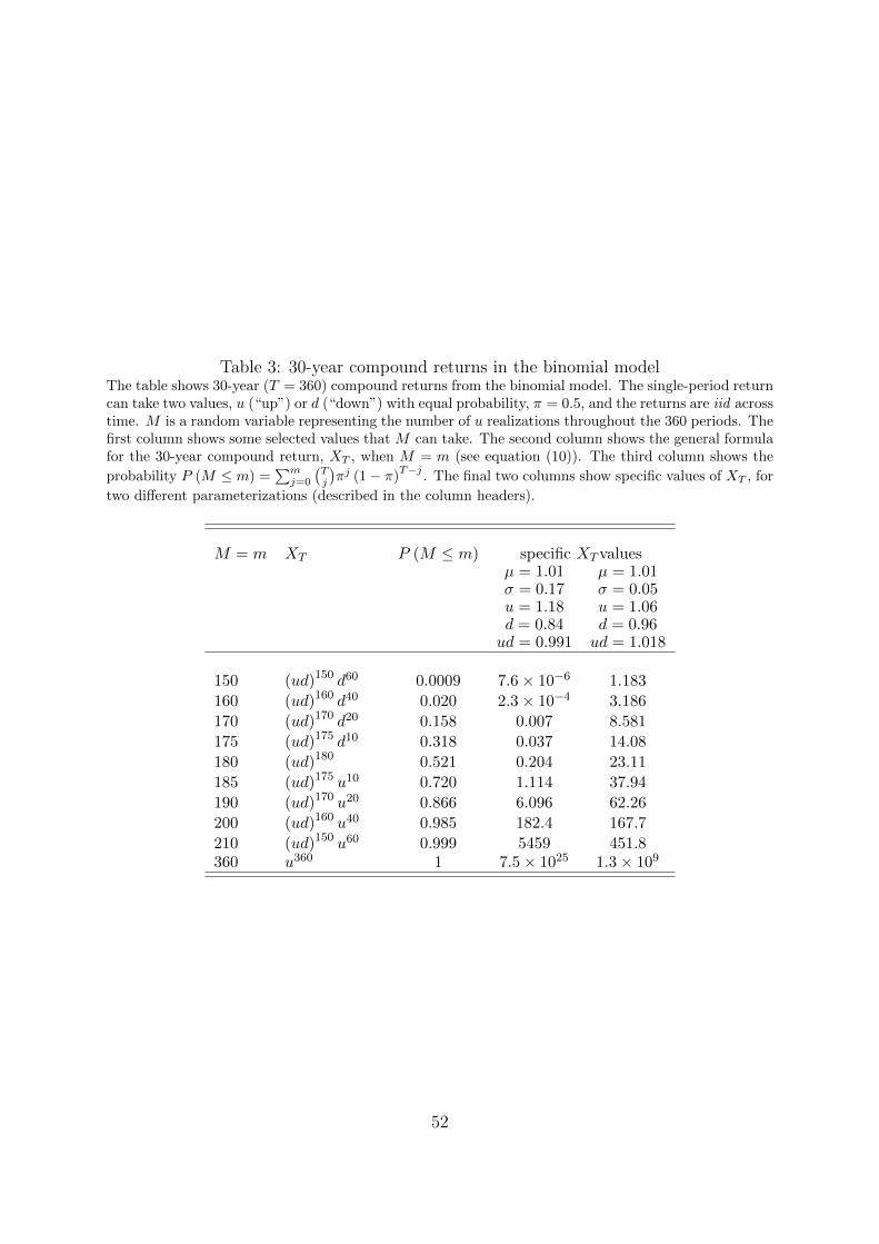
Table 3: 30-year compound returns in the binomial modelThe table shows 30-year (T = 360) compound returns from the binomial model. The single-period returncan take two values, u (“up”) or d (“down”) with equal probability, π = 0.5, and the returns are iid acrosstime. M is a random variable representing the number of u realizations throughout the 360 periods. Thefirst column shows some selected values that M can take. The second column shows the general formulafor the 30-year compound return, XT , when M = m (see equation (10)). The third column shows the

probability P (M ≤ m) =∑mj=0

(Tj

)πj (1− π)

T−j. The final two columns show specific values of XT , for

two different parameterizations (described in the column headers).

M = m XT P (M ≤ m) specific XTvaluesµ = 1.01 µ = 1.01σ = 0.17 σ = 0.05u = 1.18 u = 1.06d = 0.84 d = 0.96ud = 0.991 ud = 1.018

150 (ud)150 d60 0.0009 7.6× 10−6 1.183

160 (ud)160 d40 0.020 2.3× 10−4 3.186

170 (ud)170 d20 0.158 0.007 8.581

175 (ud)175 d10 0.318 0.037 14.08

180 (ud)180 0.521 0.204 23.11

185 (ud)175 u10 0.720 1.114 37.94

190 (ud)170 u20 0.866 6.096 62.26

200 (ud)160 u40 0.985 182.4 167.7

210 (ud)150 u60 0.999 5459 451.8360 u360 1 7.5× 1025 1.3× 109

52

Table 4: Properties of 30-year compound returns from various strategiesThe first four columns of the table show descriptives of the single-period returns of different bootstrappedstrategies: mean (µ), standard-deviation (σ), and ψ and η calculated via equation (14). The last fourcolumns show descriptives of the 30-year compound returns from the same strategies. The columnslabeled “actual” under “%>Rf”, “%>VW”, and “%>EW” show the percent of simulated strategiesthat have higher total return than the risk-free asset and the value- or equal-weighted market portfolio,respectively, over the 30-year period. The columns labeled “implied” show the corresponding probabilitiesimplied by the log-normal approximation and the single-period parameters in the first four columns. Thebootstrap procedure is described in Appendix A and the number of simulations is set to 200,000. Thesample is the CRSP stocks and the sample period is from January 1987 to December 2016.

single-period returns 30-year returnsµ σ ψ η %>Rf %>VW %>EW

actual implied actual implied actual implied

A. Unconditional single-stock strategy1.0102 0.186 -0.0065 0.183 17.6 17.0 6.4 5.9 5.5 4.8

B. Portfolio strategies (equal-weighted)N=2 1.0103 0.145 0.0001 0.143 42.1 36.6 14.7 13.0 12.2 10.5N=5 1.0103 0.101 0.0053 0.100 76.9 69.2 28.3 28.7 22.7 21.8N=10 1.0105 0.083 0.0071 0.082 93.7 85.1 38.3 39.1 29.5 28.4N=25 1.0105 0.068 0.0082 0.068 99.8 94.0 51.2 52.3 36.5 37.7N=50 1.0105 0.063 0.0085 0.062 100.0 96.2 61.0 60.0 40.1 39.6N=100 1.0104 0.060 0.0085 0.060 100.0 96.9 71.9 61.4 43.1 45.1

C. Portfolio strategies (value-weighted)N=2 1.0093 0.133 0.0006 0.132 39.9 38.5 13.3 13.2 10.9 10.7N=5 1.0096 0.097 0.0050 0.095 70.7 67.8 24.1 24.8 19.1 20.3N=10 1.0096 0.080 0.0064 0.079 86.7 81.5 31.2 31.3 24.1 24.4N=25 1.0095 0.066 0.0074 0.065 97.0 91.5 38.0 38.6 27.5 28.8N=50 1.0093 0.059 0.0075 0.059 99.4 94.2 41.7 41.0 28.0 30.9N=100 1.0092 0.054 0.0078 0.053 100.0 96.5 44.0 42.8 26.7 33.1

53

Table 5: Properties of 30-year compound returns from various strategies (earlier samples)The table shows the same descriptive statistics as Table 4 (see the caption of Table 4), but for differentsample periods. Panel A corresponds to the 30-year period from January 1957 to December 1986, whilePanel B corresponds to the 30-year period from January 1927 to December 1956.

single-period returns 30-year returnsµ σ ψ η %>Rf %>VW %>EW

actual implied actual implied actual implied

A. Jan 1957 - Dec 1986

Unconditional single-stock strategy1.0124 0.136 0.0034 0.134 42.9 42.1 24.3 24.4 13.4 13.1

Portfolio strategies (equal-weighted)N=2 1.0122 0.105 0.0068 0.103 69.9 64.2 41.4 40.5 21.0 20.6N=5 1.0124 0.080 0.0093 0.079 94.0 86.0 65.7 64.5 30.3 31.2N=10 1.0124 0.069 0.0101 0.068 99.5 92.9 82.2 78.7 35.6 38.0N=25 1.0123 0.062 0.0104 0.061 100.0 95.9 96.4 87.3 40.6 39.6N=50 1.0123 0.059 0.0105 0.058 100.0 96.8 99.7 91.5 43.3 42.3N=100 1.0124 0.058 0.0107 0.057 100.0 97.6 100.0 94.3 45.4 44.2

Portfolio strategies (value-weighted)N=2 1.0114 0.099 0.0066 0.097 64.2 63.9 34.8 36.1 16.1 16.8N=5 1.0104 0.075 0.0076 0.074 83.3 76.8 44.5 45.5 15.5 16.6N=10 1.0101 0.064 0.0080 0.064 91.4 83.3 48.2 50.0 12.0 15.8N=25 1.0096 0.055 0.0080 0.055 97.4 87.1 50.0 50.6 6.0 11.2N=50 1.0095 0.051 0.0082 0.050 99.4 90.2 50.8 53.0 2.5 8.9N=100 1.0092 0.048 0.0081 0.047 99.9 90.7 51.4 50.0 0.6 5.7

B. Jan 1927 - Dec 1956

Unconditional single-stock strategy1.0145 0.163 0.0017 0.160 65.1 53.7 25.4 20.7 13.7 11.5

Portfolio strategies (equal-weighted)N=2 1.0146 0.136 0.0056 0.133 91.1 75.1 42.9 37.3 21.4 20.4N=5 1.0147 0.115 0.0082 0.113 99.8 88.9 67.4 59.5 30.6 30.4N=10 1.0150 0.107 0.0093 0.106 100.0 93.4 83.7 71.0 35.7 34.9N=25 1.0148 0.103 0.0096 0.101 100.0 95.0 97.2 80.7 41.1 41.0N=50 1.0148 0.101 0.0098 0.099 100.0 95.6 99.8 83.4 43.7 43.8N=100 1.0149 0.100 0.0100 0.098 100.0 96.0 100.0 85.7 45.8 47.9

Portfolio strategies (value-weighted)N=2 1.0123 0.122 0.0050 0.120 86.9 74.1 32.1 29.8 13.3 13.9N=5 1.0113 0.097 0.0066 0.096 97.7 87.2 36.9 38.3 10.0 15.4N=10 1.0101 0.086 0.0064 0.085 99.7 88.9 38.6 36.2 6.2 13.8N=25 1.0101 0.079 0.0070 0.078 100.0 93.3 40.4 40.6 2.0 14.3N=50 1.0100 0.074 0.0073 0.074 100.0 95.0 42.4 39.3 0.4 12.6N=100 1.0099 0.073 0.0073 0.072 100.0 95.4 44.5 46.5 0.0 13.5

54

Table 6: Number of single-stock strategies corresponding to a portfolioThe compound return on a rebalanced portfolio can be interpreted as the average of compound returnsfrom single-stock strategies formed using the constituent stocks. The table shows the number of thesesingle-stock strategies for different portfolio sizes and rebalancing frequencies. The value can be calculatedas NT/R, where N is the number of stocks in the portfolio, T is the investment horizon (in months), andR is the rebalancing frequency. The values correspond to a 30-year investment horizon (T = 360).

monthly rebalancing 1-year rebalancing 5-year rebalancing buy-and-holdR = 1 R = 12 R = 60 R = 360

N = 2 2.3× 10108 1.1× 109 64 2N = 5 4.3× 10251 9.3× 1020 1.6× 104 5N = 10 1.0× 10360 1.0× 1030 1.0× 106 10N = 50 4.3× 10611 9.3× 1050 1.6× 1010 50

55

Internet Appendix to

“Compound Returns”

Adam Farago and Erik Hjalmarsson∗

June 3, 2019

∗Both authors are at the Department of Economics and the Centre for Finance, University of Gothen-burg. Contact information: P.O. Box 640, SE 405 30 Gothenburg, Sweden. Email: adam.farago@cff.gu.seand erik.hjalmarsson@economics.gu.se.

1 Skewness under serial correlation

In this section, we analyze the effect of serial dependence on the skewness of compound

returns. Since compounding involves multiplication rather than summation, the exact

effects of serial dependence on the compound returns is extremely difficult to derive.

Therefore, we rely on a heuristic approximation based on the log-normal case. Our

results can be summarized by the following proposition:

Proposition 1 Suppose x and xt, t = 1, ..., T are log-normally distributed random vari-

ables with mean µ and variance σ2, and let XT =∏T

t=1 xt be the corresponding compound

returns. Further, let V R denote the ratio between the long-run and short-run variance of

xt, such that

V R ≡ LR.V ar (x)

V ar (x)=

∑∞j=−∞Cov (xt, xt+j)

V ar (xt). (1)

The skewness of XT in the case when the xt-s are serially correlated can be approximated

as

Skew (XT ) =

((1 +

V R× σ2

µ2

)T+ 2

)((1 +

V R× σ2

µ2

)T− 1

) 12

. (2)

Proof. Let xt be log-normally distributed with parameters ψ and η. That is, the log-

returns yt ≡ log (xt) are normally distributed with mean ψ and volatility η. Assume

further that yt follows a linear (infinite moving average) process, such that

yt = ψ + ut, (3)

and

ut = C (L) εt =∞∑j=0

cjεt−j. (4)

The innovations εt are assumed to be iid standard normal, i.e., εt ∼ N (0, 1) .

The compound return over T periods is given by XT =∏T

t=1 xt and the log-compound

returns satisfy,

YT = log (XT ) =T∑t=1

yt = ψT +T∑t=1

ut. (5)

Using the BN decomposition (Beveridge and Nelson, 1981), we can write

ut = C (L) εt = C (1) εt + εt−1 − εt, (6)

where

εt = C (L) εt =∞∑j=0

cjεt−j and cj =∞∑

s=j+1

cs . (7)

1

C (1) =∑∞

j=0 cj denotes the so-called long-run moving average coefficient. The process

YT can therefore be written as,

YT = ψT + C (1)T∑t=1

εt +T∑t=1

(εt−1 − εt) = ψT + C (1)T∑t=1

εt − εT , (8)

using the fact that∑T

t=1 (εt−1 − εt) = ε0 − εT and imposing ε0 = 0.

The BN decomposition decomposes the process into a drift component (ψT ), a mar-

tingale component(C (1)

∑Tt=1 εt

), and a transitory component (εT ). For large T , the

permanent (martingale) component has a variation that is of an order of magnitude

greater than the transitory component, and will therefore dominate the stochastic prop-

erties of YT . We can therefore write the “long-run” part of YT as

Y LRT ≡ ψT + C (1)

T∑i=t

εt ≈ YT . (9)

Since εtiid∼ N (0, 1), it follows that

∑Tt=1 εt ∼ N (0, T ) and Y LR

T ∼ N(ψT,C (1)2 T

). Thus,

from the definition of the log-normal distribution, eYLRT ∼ LN

(ψT,C (1)2 T

). That is,

since log (XT ) = YT ≈ Y LRT , XT ≈ LN

(ψT,C (1)2 T

). The parameters ψT and C (1)2 T

pin down the distribution, and therefore also the skewness, of the compound returns as

discussed previously.

In order to assess the effects of serial dependence on compound returns vis-a-vis the

iid setting, consider the case where ut is iid. In this case, log (XT ) = Y LRT ∼ N (ψT, η2T ),

where the equality between log (XT ) and Y LRT is now exact. Compared to the serially

correlated case, the mean parameter of the distribution of Y LRT is the same, but the

variance is different. The effect of the serial dependence is therefore summarized by the

differences between the variance of Y LRT in the serially correlated case, and the variance

of Y LRT in the iid case.

Note that the (short-run) variance of yt is given by,

η2 = V ar (yt) = V ar (ut) =∞∑j=0

c2j , (10)

and the so-called long-run variance of yt is given by

LR.V ar (yt) ≡∞∑

j=−∞

Cov (yt, yt+j) = C (1)2 =

(∞∑j=0

cj

)2

. (11)

The variance of Y LRT in the iid case is thus equal to T × V ar (yt), whereas the variance

of Y LRT in the serially correlated case is equal to T × LR.V ar (yt). Define the variance

2

ratio, of the long-run variance of yt over its short-run variance,

V R ≡ LR.V ar (yt)

V ar (yt)=

(∑∞j=0 cj

)2∑∞j=0 c

2j

. (12)

A given serial correlation structure {cj}∞j=0 reduces or increases the long-run variance of

yt, relative to the iid case, by a factor given in the expression above. The impact of

serial correlation on skewness in compound returns is therefore evaluated by comparing

the skewness implied for compound returns when using the short-run variance and the

skewness implied when using the long-run variance.

The variances in equation (12) correspond to log-returns, yt, whereas the inputs

into the skewness formula in Corollary 1 of the main text correspond to variances of

simple returns, xt. Since xt ∼ LN (ψ, η2), the relationship between the parameter η2

and V ar (x) = σ2 is given by σ2 = µ2(eη

2 − 1)

, where µ = E [x]. Defining σ2V R ≡

µ2(eV Rη

2 − 1)

and using the first-order Taylor approximation eV Rη2 − 1 ≈ V Rη2 (which

is a good approximation, since the typical values of η2 in our context are close to zero),

it can be shown thatσ2V R

σ2=eV Rη

2 − 1

eη2 − 1≈ V Rη2

η2= V R .

That is, σ2V R ≈ V Rσ2. As the log-variance shifts by a factor V R, so does the variance of

simple returns, up to a first order approximation. In order to assess the effect of serial

correlation on skewness, one can therefore also equally well calculate the variance ratio

of the simple returns, rather than for the log-returns.

Finally, applying Corollary 1 of the main text to the log-normal case, it can be shown

that if xt ∼ LN (ψ, η2), then

Skew (XT ) =

((1 +

σ2

µ2

)T+ 2

)((1 +

σ2

µ2

)T− 1

) 12

. (13)

For a specific variance ratio, V R (calculated from either simple returns or log-returns),

skewness of the compound returns can be calculated as in equation (2).

There is a large literature suggesting that returns are mean-reverting over longer

horizons, which implies that V R < 1 (see, for instance, Fama and French (1988), Poterba

and Summers (1988), Cecchetti, Lam, and Mark (1990), Cutler, Poterba, and Summers,

(1991), Siegel (2008), and Spierdijk, Bikker, and van den Hoek (2012)).1

1The presence of mean reversion in stock returns is not universally accepted, however, and otherstudies argue against it; for instance, Richardson and Stock (1989), Kim, Nelson, and Startz (1991), andRichardson (1993).

3

Proposition 1 essentially implies that if single-period returns have mean µ, volatility σ,

and are non-iid, the skewness of the resulting compound returns behaves as if the single-

period returns were iid with mean µ and volatility√V R×σ. If, for example, the non-iid

single period returns have σ = 0.17 and V R = 0.8, the resulting Skew (Xt) can be well

approximated by the iid formula with volatility parameter equal to√

0.8×0.17 ≈ 0.152.2

Figure A1 illustrates the effects of serial dependence on the skewness of compound

returns. The effects of V R = 0.9 and V R = 0.8 are compared to the benchmark iid

case within each panel, and the volatility of the single-period returns is varied across

the panels. The conclusions are similar to those obtained when looking at the effect of

single-period skewness. When σ is low, the effect of serial dependence on long-horizon

skewness is small. When σ is high, the effect of serial dependence can be sizable, but only

in the range of extreme skewness levels, where interpretation of the different skewness

values is not straightforward any more. To that extent, the effect of serial dependence is

of second order importance compared to the effect of single-period return volatility.

2 Properties of skewness and quantile estimates

2.1 Skewness estimation

In this section, we explore the distribution of the skewness estimator

g ≡1n

∑ni=1 (zi − z)3(

1n

∑ni=1 (zi − z)2) 3

2

. (14)

As discussed in the main text, Wilkins (1944) shows that there is an upper limit to the

absolute value of g, which depends solely on the sample size n:

|g| ≤ n− 2√n− 1

. (15)

We focus on the estimation of skewness for long-horizon compound returns from indi-

vidual stocks, because in this case, as we will see, the estimator g becomes problematic.

We start with a Monte Carlo simulation to show the finite sample distribution of the

estimator. Later we also derive its asymptotic distribution.

For the simulation exercise, we assume that the monthly return, x, is log-normal and

2In practical applications, the long-run variance of xt can be estimated through various estimators.The long-run variance is equal to the sum of all autocovariances and can be estimated by essentiallycalculating a sample analogue of LR.V ar (xt) =

∑∞j=−∞ Cov (xt, xt+j), as in the Newey and West (1987)

estimator. The long-run variance is also equal to 2πfxt (0), where fxt (·) is the spectrum, or spectraldensity, of xt, and one can form an estimator as the average periodogram (sample spectrum) acrossfrequencies close to zero. Recent work by Muller and Watson (2017, 2018), and Lazarus, Lewis, Stock,and Watson (2016) suggest that long-run (or low-frequency) components of the data are most efficientlyextracted by considering a small set of frequencies or basis components around the zero frequency.

4

set the mean and volatility to µ = 1.01 and σ = 0.17, respectively.3 The horizon is set to

30 years, i.e., T = 360. For a given sample size n, we carry out the following simulation:

1. Simulate iid realizations of xt for t = 1, ..., T and calculate the 30-year compound

return using these monthly return realizations.

2. Repeat step (1) n times to get a sample of compound returns (with sample size n),

and estimate the skewness of the compound returns using the estimator g.

3. Repeat steps (1) and (2) 10,000 times to get a sample of the skewness estimates.

Panels A and B of Figure A2 show the distribution of the skewness estimates for two

sample sizes, n = 20, 000 and n = 200, 000. The vertical line on each graph represents the

upper limit of g from equation (15). With the distributional assumptions on the single-

period return used for the simulation, the skewness of the 30-year compound returns is

3.6 × 106 according to Proposition 1 of the main text. Therefore, the upper limit of

the estimator g, which is 141.4 for n = 20.000 (Panel A of Figure A2) and 447.2 for

n = 200, 000 (Panel B of Figure A2), is clearly binding and the estimator g is severely

downward biased.

In order for the upper limit on g not to be binding and to possibly estimate a skewness

of 3.6 × 106, a sample of n ≥ 1.13 × 1013 would be needed. Since it is not feasible to

provide simulation evidence for such a large sample size, we turn to asymptotic results.

Let the k-th central moment of the variable z be denoted by µk, and its sample analogue

by mk, i.e.,

µk ≡ E[(z − E [z])k

]and mk ≡

1

n

n∑i=1

(zi − z)k . (16)

Then the skewness of z, and its estimator from equation (14), g, are defined as

Skew (z) =µ3

µ3/22

and g =m3

m3/22

. (17)

Provided the third moment of z exists, m2 and m3 trivially converge to µ2 and µ3,

respectively, by a law of large numbers. Further, from Serfling (1980, page 72), as n→∞,

√n

[m2 − µ2

m3 − µ3

]d→ N

([0

0

],

µ4 − µ22 µ5 − 4µ2µ3

µ5 − 4µ2µ3 µ6 − µ23 − 6µ2µ4 + 9µ3

2

). (18)

3We could have used any distributional assumption for the single-period returns. We chose thelog-normal distribution so that the results are comparable with our discussion on quantiles in InternetAppendix 2.2. The conclusions are qualitatively the same if we use the normal distribution or a moreskewed distribution for the single-period returns.

5

By the delta method, and provided the sixth moment of z exists, g satisfies

√n (g − Skew(z))

d→ N

(0,

1

µ32

(µ6 − 6µ2µ4 + 9µ3

2 − µ23

)− 3

µ3

µ42

(µ5 − 4µ2µ3) +9

4

µ23

µ52

(µ4 − µ2

2

)).(19)

That is, the skewness estimator g is consistent and asymptotically normally distributed,

with an asymptotic variance that is a function of the central moments up to order 6.4

As is implied by Proposition 1 of the main text, the skewness (and other higher order

moments) in compound returns can be extremely large at long horizons. The higher-order

moments present in the variance formula for g in equation (19) is therefore a warning

sign that the variance of the skewness estimator (based on the asymptotic approximation)

might be very large for long-horizon compound returns.

Panel A of Figure A3 shows two-standard error bounds of the skewness estimator, as

a function of the horizon on which returns are compounded, for sample sizes n = 20, 000,

n = 200, 000, and n = 1016. The standard errors are calculated via the asymptotic

approximation in equation (19) using the assumption of iid log-normally distributed one-

period returns with µ = 1.01 and σ = 0.17.5 The two-standard error bounds on the

skewness estimator widen very quickly with the horizon. As shown in the previous simu-

lation exercise, the actual distribution of g is very far from the asymptotic approximation

for the sample sizes n = 20, 000 and n = 200, 000 (see Panels A and B of Figure A2), so

let us focus on the case when the sample size is much larger. For n = 1016, the upper limit

from equation (15) is not binding and the estimator g should be mostly unbiased if its

actual distribution is close to the asymptotic approximation in equation (19). However,

as seen in Panel A of Figure A3, the skewness estimator is still essentially uninformative

for horizons of 10 years or more due to the large standard errors of the estimator.

Overall, the results in this section show that in the case of individual stocks, direct

estimation of the skewness, in returns compounded over 10 or more years, is next to

meaningless. For practically relevant sample sizes, the estimator is severely downward

biased, while for considerably larger sample sizes (if they were practically feasible), the

enormous standard errors make the estimates highly unreliable.

4The asymptotic normality result in Serfling (1980) is derived for the iid case, although the resultshould extend to more general cases as long as sufficient conditions for a central limit theorem apply.

5The asymptotic approximation can be applied to any distribution for the single-period returns wherethe first 6 central moments are known. The log-normal distribution is used for illustration so that theresults are comparable with our discussion on quantiles in Internet Appendix 2.2. The conclusions arequalitatively the same if we use the normal distribution or a more skewed distribution for the single-period returns. When x ∼ LN

(ψ, η2

), the non-central moments are given by E

[xk]

= ekψ+12k

2η2 , andthe central moments can be calculated from the non-central moments. The central moments for theproduct process XT can then be obtained via the formula in Proposition 1. Finally, using the centralmoments of XT in the variance formula from (19) provides the standard error estimates used in Panel Aof Figure A3.

6

2.2 Quantile estimation

The general formula for the sample quantile is given by

qα ≡ inf

{w :

1

n

n∑i=1

I {zi ≤ w} ≥ α

}. (20)

The asymptotic distribution of qα, as n→∞, is given by

√n (qα − qα)

d→ N

(0,α (1− α)

f 2z (qα)

), (21)

where fz (·) is the density of the random variable z (Serfling, 1980). Using the iid log-

normal assumption on the single-period returns (with µ = 1.01 and σ = 0.17), Panels B to

D in Figure A3 show quantiles of the distribution of compound returns as a function of the

horizon, together with the two-standard error bounds of qα for sample sizes n = 20, 000

and n = 200, 000. The standard errors are calculated using the asymptotic approximation

in (21), and Panels B, C, and D correspond to α levels of 0.9, 0.99, and 0.999, respectively.

The results in Figure A3 reveal that the two-standard error bounds for the quantile

estimates are considerably narrower than in the case of the skewness estimator. In general,

the standard error of the quantile estimator increases with the horizon, and is larger

for quantiles far out into the tail. However, even for the 99.9-th percentile of the 30-

year compound returns (Panel D), qα is fairly precisely estimated with a sample size of

n = 200, 000, in large contrast to the skewness estimator in Panel A.

The results in Figure A3 show that based on the asymptotic approximation in equa-

tion (21), the quantiles of long-horizon compound returns can be fairly precisely esti-

mated. However, as seen in the case of the skewness estimator, the asymptotic approxi-

mation can be far away from the actual distribution of the estimator. To show that this

is not the case for the quantile estimates, we carry out the same simulation exercise as

in the beginning of Section 2.1 to get the finite sample distribution of qα. The results

are reported in Panels C to F of Figure A2 for the α = 0.99 and α = 0.999 quantiles

(we would expect more discrepancies for quantiles far out in the tail). The histograms

represent the distribution from the Monte Carlo simulation, while the solid lines show

the corresponding asymptotic approximation from equation (21). The simulated finite

sample distributions are close to their asymptotic counterparts, especially for the larger

sample size (n = 200, 000).

3 Quantile based skewness measures

Moment based measures of skewness are not the only way to describe the asymmetry of a

return distribution. Kim and White (2004) advocate the use of quantile based measures of

7

skewness because they are (much) more robust to the presence of outliers. In particular,

consider

ζα ≡qα + q1−α − 2q0.5

qα − q1−α. (22)

Bowley (1920) proposed the above coefficient as a measure of skewness with α = 0.75 (i.e.,

using quartiles), and Hinkley (1975) proposed the generalization to use any α between

0.5 and 1. It is easy to see that for any symmetric distribution, ζα = 0. Unlike γ,

the coefficient ζα is bounded with the maximum value of 1 representing extreme right

skewness and the minimum value -1 indicating extreme left skewness.

When x is a log-normal random variable, x ∼ LN(ψ, η2), then ζα can be calculated

as

ζα =eψ+ηΦ−1(α) + eψ−ηΦ−1(α) − 2eψ

eψ+ηΦ−1(α) − eψ−ηΦ−1(α), (23)

where Φ−1 denotes the inverse cdf of the standard normal distribution. However, we need

a more flexible distribution to be able to study the effects of the higher order moments

of the single-period returns on the distribution of compound returns.

The Normal Inverse Gaussian (NIG) distribution, introduced by Barndorff-Nielsen

(1997), is a four-parameter distribution allowing for non-zero skewness and fat tails. The

pdf of a random variable z ∼ NIG (ϕ, β, ν, δ) is

f (z) =ϕδ exp (δλ+ β(z − ν))

π√δ2 + (z − ν)2

K1

(ϕ

√δ2 + (z − ν)2

), (24)

where ϕ, β, ν, and δ are the parameters of the distribution, λ ≡√ϕ2 − β2 and K1 is

the modified Bessel function of the third kind. The parameters have to obey |β| < ϕ

(implying λ > 0). The moment-generating function of the distribution is

E [exp (kz)] = exp

(kν + δ

(λ−

√ϕ2 − (β + k)2

)). (25)

The first four moments are

E [z] = ν+δβ

λ, V ar (z) = δ

ϕ2

λ3 , Skew (z) = 3β

ϕ√δλ

, Kurt (z) = 3+3

δλ

(1 + 4

β2

ϕ2

).

(26)

As is seen above, the parameter β captures asymmetry: β = 0 implies zero skewness, while

β < 0 (β > 0) leads to negative (positive) skewness. Note that the normal distribution

(with mean µ and volatility σ) is nested in the NIG distribution with ν = µ, β = 0,

δ → ∞, ϕ → ∞, and δϕ

= σ2. Another convenient feature of the distribution is that it

is closed under convolution in the following sense: if z1, z2, ..., zT are iid NIG (ϕ, β, ν, δ)

8

variables with parameters, then

T∑t=1

zt ∼ NIG (ϕ, β, Tν, Tδ) . (27)

Let us assume that zt ∼ NIG (ϕ, β, ν, δ) are iid for t = 1, ..., T , and the single-

period (e.g., monthly) gross return on an asset or portfolio is xt ≡ exp (zt). That is,

single-period gross returns follow a log-NIG distribution. Note that since the normal

distribution is a special case of the NIG distribution, the log-normal distribution is a

special case of the log-NIG distribution. The first four non-central moments of xt are

given by equation (25), since E[xkt]

= E [exp (kzt)]. The compound return over T

periods is XT =∏T

t=1 xt = exp(∑T

t=1 zt

), which also follows a log-NIG distribution as

implied by equation (27). To study how the quantile based skewness measure ζα behaves

in the case of compound returns, we follow these steps:

1. Assume that the first four moments of the single-period gross return, xt, are given.

2. Translate E[xt], Std(xt), Skew(xt), and Kurt(xt) into the corresponding non-

central moments E[xkt ] for k = 1, 2, 3, 4.

3. Find the parameters of the corresponding random variable zt ∼ NIG (ϕ, β, ν, δ),

by numerically solving the set of four equations given by (25) for k = 1, 2, 3, 4.

4. The quantile qα

(∑Tt=1 zt

)can be found numerically by using the pdf given in

equation (24), where the distribution of∑T

t=1 zt is given in (27).

5. Quantiles of the compound return distribution (over horizon T ) are given by qα (XT ) =

exp(qα

(∑Tt=1 zt

)), and ζα can be calculated from the quantiles via equation (23).

Figure A4 shows how ζα of compound returns changes with the horizon for α =

0.75 (Panels A and C) and α = 0.9 (Panels B and D). Several single-period return

distributions, as described by the first four moments, are considered. The expected single-

period return is always kept at E[xt] = 1.01. The volatility of the single-period return

varies across the panels with Std(xt) = 0.05 (Panels A and B) or Std(xt) = 0.17 (Panels

C and D). Three scenarios regarding the asymmetry and fat-tails of the single-period

return distribution are considered within each graph, corresponding to (i) Skew (xt) = 0

and Kurt(xt) = 5, (ii) Skew (xt) = 1 and Kurt(xt) = 10, and (iii) Skew (xt) = 2 and

Kurt(xt) = 20.

There are two conclusions from Figure A4 that we would like to highlight. First, ζα

increases with the horizon in all graphs, which implies that compound returns become

more asymmetric as the horizon increases. Second, the dominant factor in determining

the asymmetry of long-run compound returns is the volatility of the single-period returns,

9

and higher order moments (skewness and kurtosis) of the single-period return distribution

have only a second order effect. For horizons over ten years (T ≥ 120), the value of ζα

varies much more across the graphs (corresponding to changes in Std(xt)) than within

the graphs (corresponding to changes in Skew(xt) and Kurt(xt)) for a fixed level of α.

These conclusions are the same as those in the main text.

4 Details for Appendix C.1 of the main text

The joint distribution of the random variables (Luu, Lud, Ldu, Ldd) is a multinomial dis-

tribution and has the pmf

P (Luu = luu, Lud = lud, Ldu = ldu, Ldd = T − luu − lud − ldu)

=T !

luu!lud!ldu! (T − luu − lud − ldu)!πluuuu (π − πuu)lud+ldu (1− 2π + πuu)

T−luu−lud−ldu(28)

Using (28),

P (Lud = lud, Ldu = ldu) =

T−lud−ldu∑luu=0

P (Luu = luu, Lud = lud, Ldu = ldu, Ldd = T − luu − lud − ldu)

=

T−lud−ldu∑luu=0

T !

luu!lud!ldu! (T − luu − lud − ldu)!πluuuu (π − πuu)lud+ldu (1− 2π + πuu)T−luu−lud−ldu

=T !

lud!ldu! (T − lud − ldu)!(π − πuu)lud+ldu

T−lud−ldu∑luu=0

(T − lud − ldu)!

luu! (T − luu − lud − ldu)!πluuuu (1− 2π + πuu)T−luu−lud−ldu

=T !

lud!ldu! (T − lud − ldu)!(π − πuu)lud+ldu (1− 2π + 2πuu)T−lud−ldu ,

(29)

where we used the binomial expansion to go from line 3 to 4. Using (29),

P (Lud + Ldu = l) =

l∑lud=0

P (Lud = lud, Ldu = l − lud)

=

l∑lud=0

T !

lud! (l − lud)! (T − l)!(π − πuu)l (1− 2π + 2πuu)T−l

=T !

l! (T − l)!(1− 2π + 2πuu)T−l

l∑lud=0

l!

lud! (l − lud)!(π − πuu)l−lud (π − πuu)lud

=T !

l! (T − l)!(1− (2π − 2πuu))T−l (2π − 2πuu)l

= b (l;T, 2 (π − πuu)) ,

(30)

10

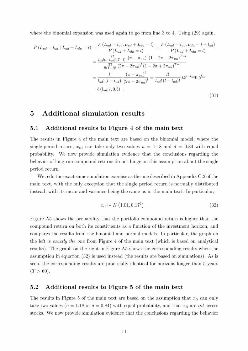
where the binomial expansion was used again to go from line 3 to 4. Using (29) again,

P (Lud = lud | Lud + Ldu = l) =P (Lud = lud, Lud + Ldu = l)

P (Lud + Ldu = l)=P (Lud = lud, Ldu = l − lud)

P (Lud + Ldu = l)

=

T !lud!(l−lud)!(T−l)! (π − πuu)l (1− 2π + 2πuu)T−l

T !l!(T−l)! (2π − 2πuu)l (1− 2π + 2πuu)T−l

=l!

lud! (l − lud)!(π − πuu)l

(2π − 2πuu)l=

l!

lud! (l − lud)!0.5l−lud0.5lud

= b (lud; l, 0.5) .

(31)

5 Additional simulation results

5.1 Additional results to Figure 4 of the main text

The results in Figure 4 of the main text are based on the binomial model, where the

single-period return, xti, can take only two values u = 1.18 and d = 0.84 with equal

probability. We now provide simulation evidence that the conclusions regarding the

behavior of long-run compound returns do not hinge on this assumption about the single

period return.

We redo the exact same simulation exercise as the one described in Appendix C.2 of the

main text, with the only exception that the single period return is normally distributed

instead, with its mean and variance being the same as in the main text. In particular,

xti ∼ N(1.01, 0.172

). (32)

Figure A5 shows the probability that the portfolio compound return is higher than the

compound return on both its constituents as a function of the investment horizon, and

compares the results from the binomial and normal models. In particular, the graph on

the left is exactly the one from Figure 4 of the main text (which is based on analytical

results). The graph on the right in Figure A5 shows the corresponding results when the

assumption in equation (32) is used instead (the results are based on simulations). As is

seen, the corresponding results are practically identical for horizons longer than 5 years

(T > 60).

5.2 Additional results to Figure 5 of the main text

The results in Figure 5 of the main text are based on the assumption that xti can only

take two values (u = 1.18 or d = 0.84) with equal probability, and that xti are iid across

stocks. We now provide simulation evidence that the conclusions regarding the behavior

11

of long-run compound returns do not hinge on the distributional assumption and that

the results are not sensitive to moderate correlation across stocks.

The graphs in the top row of Figure A6 (Panels A and B) are exactly the same as the

ones in Figure 5 of the main text. The graphs in the middle row of Figure A6 (Panels

C and D) show the corresponding results when the assumption in equation (32) is used

instead and xti are still iid across stocks. Finally, the graphs in the bottom row (Panels

E and F) show the corresponding results when the assumption in equation (32) is used

and individual stock returns are positively correlated with Corr(xti, xtj) = 0.1 for all

i 6= j. Comparing the graphs within each column (the graphs on the left correspond to

N = 10, while the graphs on the right represent N = 50), these changes in the underlying

assumptions for the single-period returns do not materially affect the results.

5.3 Additional results to Figure 6 of the main text

Figure 6 from the main text shows the probability that an equal-weighted and monthly

rebalanced portfolio of 50 stocks beats the k-th best from 1,000 stocks over a 30-year

investment horizon. The results in Figure 6 of the main text are based on the analytical

formula derived in Appendix C.3 of the main text. When deriving the analytical formula,

we assume that (i) xti can only take two values (u = 1.18 or d = 0.84) with equal

probability, (ii) xti are iid across all stocks on the market, and (iii) the portfolio is

rebalanced monthly. We additionally make the approximating assumptions that (iv) XTp

is log-normal, and (v) XTp and X∗T [k] are independent. We now provide simulation

evidence via Figure A7 to show the robustness of the results in relation to the above

assumptions. The solid (blue) line in all three graphs of Figure A7 is exactly the same as

the one in Figure 6 of the main text.

Panel A shows the effect of the approximating assumptions, (iv) and (v), on the

results. The dashed line corresponds to simulation results that do not use the approx-

imating assumptions but rely on the other three assumption, (i) to (iii). The results

remain almost identical.

Panel B shows the effect of different assumptions on the single-period return distribu-

tion. The dashed line corresponds to simulation results where xti ∼ N (1.01, 0.172) for all

i and xti are iid across stocks (i.e., (i) is changed and (iv) and (v) are relaxed compared

to the analytical results). The dash-dotted line corresponds to simulation results where

xti ∼ N (1.01, 0.172) for all i and Corr(xti, xtj) = 0.1 for all i 6= j (i.e., (i) and (ii) are

changed and (iv) and (v) are relaxed). Changing the single-period return distribution

has an almost negligible effect on the probabilities, while increasing the correlation across

stocks has a larger but still not major effect.

Panel C shows the effect of different rebalancing frequencies. The three additional

lines correspond to simulation results where xti ∼ N (1.01, 0.172) for all i, xti are iid

12

across stocks, and the portfolio is rebalanced once a year (dashed line), rebalanced once

every five years (dash-dotted line), or not rebalanced (dotted line), i.e., assumptions (i)

and (iii) are changed and (iv) and (v) are relaxed. Reducing the rebalancing frequency

from one month to five years has a relatively small effect on the probabilities. However,

as the results corresponding to the buy-and-hold portfolio show, completely getting rid

of rebalancing does have a considerable effect.

Overall, the results from Figure A7 suggest that (i) the approximating assumptions

used for the analytical formula are fairly accurate, (ii) the results do not hinge on the

particular choice of the single-period return distribution or moderate changes of the cor-

relation across stocks, and (iii) the results are fairly robust to the rebalancing frequency

of the portfolio as long as there is some rebalancing (at least once every 5 years in our

example).

5.4 Additional results to Figure 7 of the main text

Figure 7 of the main text shows the probability that an equal-weighted and monthly

rebalanced portfolio of 50 stocks beats the equal-weighted and monthly rebalanced market

portfolio (of 1,000 stocks) over the investment horizon T . The analytical results presented

in Figure 7 of the main text are based on the log-normal approximation, which works well

if both the market portfolio and the 50-stock portfolio are rebalanced frequently (e.g.,

every month). We now provide simulation evidence via Figure A8 to show how the results

change in case of less frequent rebalancing of the 50-stock portfolio, or if the benchmark

is the buy-and-hold market portfolio.

Panels A and B of Figure A8 correspond to the case when the benchmark is the

monthly rebalanced market portfolio. The solid (blue) line in Panels A and B are exactly

the same as the corresponding results from Figure 7 of the main text. The rest of the

lines present simulation results, where xti ∼ N (1.01, 0.172) for all stocks i on the market,

Corr(xti, xtj) = ρ for all i 6= j (with ρ = 0 in Panel A and ρ = 0.1 in Panel B), and the

portfolio is rebalanced once a year, once every 5 years, or not rebalanced at all. Reducing

the rebalancing frequency from monthly to yearly barely changes the probability that

the portfolio of 50 stocks beats the market portfolio over horizon T . If the portfolio

is only rebalanced once every five years, the probability that the portfolio beats the

market becomes somewhat lower, but the change is not substantial. For example, when

ρ = 0.1 (Panel B), there is a 41.7% chance that the monthly rebalanced portfolio beats

the (equal-weighted and monthly rebalanced) market portfolio on a 30-year horizon, while

the corresponding probability for the portfolio that is rebalanced every 5 years is 37.0%. If

the portfolio is not rebalanced at all, the probability that the portfolio beats the market

gets considerably lower over long horizons: e.g., the corresponding probability for the

buy-and-hold portfolio is 17.6%, which is less than half of what 5-yearly rebalancing can

13

achieve. A comparison of Panels A and B reveals that the results are not sensitive to

moderate changes in the correlation across stocks on the market.

Panels C and D of Figure A8 correspond to the case when the benchmark is the

buy-and-hold market portfolio. At the initial time period, the market portfolio is equal-

weighted, but for later periods the weights in the market portfolio depend on past returns

of the individual stocks (there is no rebalancing), and the market portfolio can be viewed

as the value-weighted portfolio. Since all stocks are ex ante identical, the lowest variance is

achieved by the equal-weighted market portfolio, and the variance of the value-weighted

portfolio will be higher. Consequently, the 50-stock portfolios (rebalanced at various

frequencies) will have a better chance of beating the buy-and-hold market portfolio in

the long-run than the monthly rebalanced market portfolio. For example, when ρ = 0.1

(Panel D), there is a 62.8% chance that the monthly rebalanced portfolio beats the (buy-

and-hold) market portfolio on a 30-year horizon. Reducing the rebalancing frequency all

the way to rebalancing only once every five years does not have a substantial effect on

the probability of beating the market. If the portfolio is only rebalanced once every five

years, the probability that the portfolio beats the (buy-and-hold) market on a 30-year

horizon is still 54.7%. A comparison of Panels C and D reveals that the results are not

sensitive to moderate changes in the correlation across stocks on the market.

14

References

Barndorff-Nielsen, O.E., 1997. Normal Inverse Gaussian Distributions and StochasticVolatility Modelling, Scandinavian Journal of Statistics 24, 1-13.

Bowley, A.L., 1920. Elements of Statistics, Scribner’s, New York, USA.

Cecchetti, S.G., P.S. Lam, and N.C. Mark, 1990. Mean Reversion in EquilibriumAsset Prices, American Economic Review 80, 398-418.

Cutler, D.M., J.M. Poterba, and L.H. Summers, 1991. Speculative Dynamics. Reviewof Economic Studies 58, 529-546.

Fama, E., and K. French, 1988. Permanent and Temporary Components of StockPrices. Journal of Political Economy 96, 246-273.

Hinkley, D.V., 1975. On Power Transformations to Symmetry. Biometrika 62, 101-111.

Kim, M.J., C.R. Nelson, and R. Startz, 1991. Mean Reversion in Stock Prices? AReappraisal of the Empirical Evidence, Review of Economic Studies 58, 515-528.

Kim, T.-H., H. White, 2004. On More Robust Estimation of Skewness and Kurtosis,Finance Research Letters 1, 56-73.

Lazarus, E., D.J., Lewis, J.H., Stock, and M.W. Watson, 2016. HAR Inference:Kernel Choice, Size Distortions, and Power Losses, Working Paper, Harvard University.

Muller, U.K., and M.W. Watson, 2017. Low-Frequency Econometrics. In Advancesin Economics and Econometrics: Eleventh World Congress of the Econometric Society,Volume II, editors B. Honore and L. Samuelson, Cambridge University Press, 53-94.

Muller, U.K., and M.W. Watson, 2018. Long-Run Covariability. Econometrica 86,775-804.

Newey, W., and K. West, 1987. A Simple, Positive Semi-Definite, Heteroskedasticityand Autocorrelation Consistent Covariance Matrix. Econometrica 55, 703-708.

Poterba, J., and L.H. Summers, 1988. Mean Reversion in Stock Prices: Evidence andImplications, Journal of Financial Economics 22, 27-59.

Richardson, M., 1993. Temporary Components of Stock Prices: A Skeptic’s View,Journal of Business and Economics Statistics 11, 199-207.

Richardson, M., and J. Stock, 1989. Drawing Inferences from Statistics Based onMultiyear Asset Returns, Journal of Financial Economics 25, 323-348.

Serfling, R.J., 1980. Approximation Theorems of Mathematical Statistics. John Wiley& Sons, New York, USA.

Siegel, J.J., 2008. Stocks for the Long Run. McGraw Hill, New York.

15

Spierdijk, L., J.A. Bikker, and P. van den Hoek, 2012. Mean Reversion in InternationalStock Markets: An Empirical Analysis of the 20th Century, Journal of InternationalMoney and Finance 31, 228-249.

Wilkins, J.E., 1944. A note on skewness and kurtosis. Annals of Mathematical Statis-tics 15, 333-335.

16

Figure A1: Skewness of compound returns - the effect of serial correlationThe graphs show the skewness of compound returns as a function of the compounding horizon, T , when

single-period returns might be serially correlated. The values are calculated using equation (2). The

single-period gross return is assumed to be log-normal with mean µ = 1.01 and standard deviation σ

that varies across the panels (see above each panel). The lines correspond to cases where single-period

returns are independent across time (iid), or are serially correlated (V R = 0.9 or 0.8). VR is the ratio

between the long-run and short-run variance of the single-period return, defined via equation (12).

A. σ = 0.05 B. σ = 0.08

12 60 120 180 240 300 360

0

5

10

15

20

12 60 120 180 240 300 360

0

5

10

15

20

C. σ = 0.11 D. σ = 0.17

12 60 120 180 240 300 360

0

5

10

15

20

12 60 120 180 240 300 360

0

5

10

15

20

17

Figure A2: Distribution of the skewness and quantile estimators in finite samplesThe histograms in these graphs represent the distribution of skewness estimates (Panels A and B) and

quantile estimates (Panels C to F) of 30-year (T = 360) compound returns from individual stocks. The

single-period (monthly) gross returns are assumed to be iid log-normal with mean µ = 1.01 and volatility

σ = 0.17. The histograms are the results of Monte Carlo simulations described in Internet Appendix 2.1.

The distribution of the skewness and quantile estimates correspond to two sample sizes, n = 20, 000

(panels on the left) and n = 200, 000 (panels on the right). The vertical lines in the two top graphs

correspond to the upper limit on the skewness estimator in equation (15). The curves in Panels C to F

are based on the asymptotic distribution of the quantile estimates in equation (21).

A. Skewness, n = 20, 000 B. Skewness, n = 200, 000

g

0 50 100 150 200

←

n − 2√

(n − 1)

g

0 100 200 300 400 500 600

←

n − 2√

(n − 1)

C. Quantile, α = 0.99 , n = 20, 000 D. Quantile, α = 0.99, n = 200, 000

qα

250 300 350 400 450 500

qα

340 360 380 400 420

E. Quantile, α = 0.999, n = 20, 000 F. Quantile, α = 0.999, n = 200, 000

qα

1000 2000 3000 4000 5000 6000 7000 8000

qα

3500 4000 4500 5000

18

Figure A3: Asymptotic two-standard error bounds for skewness and quantile estimatorsThe graphs show two-standard error bounds of the skewness estimator (in Panel A) and quantile estimator

(in Panels B to D for various α-quantiles), as a function of the horizon over which the underlying returns

are compounded, for different sample sizes (see legends). In all the graphs, the solid line shows the

skewness or quantile of the compound returns. The other lines show the two-standard error bounds, for

which the standard errors are calculated via the asymptotic approximation (equation (19) for skewness

and equation (21) for the quantiles). It is assumed that single period returns are iid log-normally

distributed with mean µ = 1.01 and volatility σ = 0.17.

A. Skewness B. Quantile, α = 0.9

12 60 120 180 240 300 360

0

1000

2000

3000

4000

5000

12 60 120 180 240 300 360

0

5

10

15

C. Quantile, α = 0.99 D. Quantile, α = 0.999

12 60 120 180 240 300 360

0

100

200

300

400

500

12 60 120 180 240 300 360

0

1000

2000

3000

4000

5000

6000

7000

19

Figure A4: Quantile based measures of skewnessThe graphs show the quantile-based skewness coefficient of compound returns, ζα (defined in equa-

tion (22)), as a function of the compounding horizon, T , when single-period returns are iid. The values

are calculated using the steps described on page 9. The expected value of the single-period gross return

is µ = 1.01 in all cases, the volatility of the single-period return, σ, is varied across the panels (see

above each panel), while different single-period skewness and kurtosis combinations are represented by

the different lines (see legends).

A. σ = 0.05 and α = 0.75 B. σ = 0.05 and α = 0.9

12 60 120 180 240 300 360

0

0.2

0.4

0.6

0.8

1

12 60 120 180 240 300 360

0

0.2

0.4

0.6

0.8

1

C. σ = 0.17 and α = 0.75 D. σ = 0.17 and α = 0.9

12 60 120 180 240 300 360

0

0.2

0.4

0.6

0.8

1

12 60 120 180 240 300 360

0

0.2

0.4

0.6

0.8

1

20

Figure A5: Probability that a portfolio of two stocks beats its constituentsThe figure shows the probability that the total compound return on the equal-weighted and monthly

rebalanced portfolio of N = 2 stocks is higher than the compound return on its best performing con-

stituent. The graph on the left is exactly the same as Figure 4 of the main text (see the caption there for

details), where the single-period (monthly) gross return on stock i in period t, xti, can take two values,

u = 1.18 or d = 0.84 with equal probability. The graph on the right shows corresponding results, based

on simulations, when xti ∼ N(1.01, 0.172

)instead.

A. Binomial B. Normal

12 60 120 180 240 300 360

0

0.2

0.4

0.6

0.8

12 60 120 180 240 300 360

0

0.2

0.4

0.6

0.8

21

Figure A6: Probability of the portfolio beating its constituents at a 30-year horizonThe graphs show the probability that the total compound return on the equal-weighted portfolio of N

stocks is higher than the compound return on its k-th best performing constituent. The graphs in Panels

A and B are exactly the same as the ones in Figure 5 of the main text (see the caption there for details),

where the single-period (monthly) gross return on stock i in period t, xti, can take two values, u = 1.18

or d = 0.84 with equal probability, and xti are independent across stocks. The graphs in the rest of the

panels (C to E) show corresponding results when xti ∼ N(1.01, 0.172

)instead. In Panels C and D xti

are independent across stocks. In Panels E and F Corr(xti, xtj) = 0.1 for all i 6= j. The results in all

graphs are based on simulations.

A. Binomial, N = 10 B. Binomial, N = 50

1 2 3 4 5 6 7 8 9 10

0

0.2

0.4

0.6

0.8

1

1 3 5 7 9 11 13 15 17 19

0

0.2

0.4

0.6

0.8

1

C. Normal, N = 10 D. Normal, N = 50

1 2 3 4 5 6 7 8 9 10

0

0.2

0.4

0.6

0.8

1

1 3 5 7 9 11 13 15 17 19

0

0.2

0.4

0.6

0.8

1

E. Correlated normal, N = 10 F. Correlated normal, N = 50

1 2 3 4 5 6 7 8 9 10

0

0.2

0.4

0.6

0.8

1

1 3 5 7 9 11 13 15 17 19

0

0.2

0.4

0.6

0.8

1

22

Figure A7: Probability of the portfolio beating the k-th best stock on the marketThe figure shows the probability that the total compound return on the equal-weighted and monthly

rebalanced portfolio of 50 stocks, Xr1Tp, is higher than the compound return on the k-th best performing

stock, X∗T (k), out of 1,000 identical stocks. The solid (blue) line in all three graphs is exactly the same

as the one in Figure 6 of the main text (based on our approximate analytical formula, see the caption

there for details). Panel A shows the effect of the approximating assumptions on the results. The

dashed line corresponds to simulation results that do not use the approximating assumptions but rely

on the same single-period return distribution (return on all stocks can take only two values u = 1.18 and

d = 0.84 with equal probability, and returns are iid across stocks). Panel B shows the effect of different

assumptions on the single-period return distribution. The dashed line corresponds to simulation results

where xti ∼ N(1.01, 0.172

)for all i and xti are iid across stocks. The dash-dotted line corresponds to

simulation results where xti ∼ N(1.01, 0.172

)for all i and Corr(xti, xtj) = 0.1 for all i 6= j. Panel C

shows the effect of different rebalancing frequencies. The non-solid lines correspond to simulation results

where xti ∼ N(1.01, 0.172

)for all i, xti are iid across stocks, and the portfolio is rebalanced once a year

(dashed line), rebalanced once every five years (dash-dotted line), or not rebalanced (dotted line).

A. Analytical vs. simulation (binomial) B. Effect of single-period distribution

20 40 60 80 100 120 140

0

0.2

0.4

0.6

0.8

1

20 40 60 80 100 120 140

0

0.2

0.4

0.6

0.8

1

C. Effect of rebalancing frequency

20 40 60 80 100 120 140

0

0.2

0.4

0.6

0.8

1

23

Figure A8: Probability of the portfolio beating the marketThe figure shows the probability that an equal weighted portfolio of 50 stocks beats the market portfolio,

consisting of 1,000 stocks, over the investment horizon T . The market portfolio is either the equal-

weighted and monthly rebalanced portfolio (Panels A and B) or the equal-weighted buy-and-hold portfolio

(Panels C and D). The solid (blue) line in Panels A and B shows the monthly rebalanced portfolio, and is

exactly the same as the corresponding lines (with the appropriate correlation across stocks) in Figure 7

of the main text. The rest of the lines correspond to simulation results where xti ∼ N(1.01, 0.172

)for

all i, Corr(xti, xtj) = ρ for all i 6= j, and the portfolio is rebalanced monthly (solid line in Panels C

and D), once a year (dashed line in all panels), rebalanced once every five years (dash-dotted line in all

panels), or not rebalanced (dotted line in all panels).

A. Rebalanced market, Corr(xti, xtj) = 0 B. Rebalanced market, Corr(xti, xtj) = 0.1

12 60 120 180 240 300 360

0

0.1

0.2

0.3

0.4

0.5

0.6

0.7

12 60 120 180 240 300 360

0

0.1

0.2

0.3

0.4

0.5

0.6

0.7

C. Buy-and-hold market, Corr(xti, xtj) = 0 D. Buy-and-hold market, Corr(xti, xtj) = 0.1

12 60 120 180 240 300 360

0

0.1

0.2

0.3

0.4

0.5

0.6

0.7

12 60 120 180 240 300 360

0

0.1

0.2

0.3

0.4

0.5

0.6

0.7

24