correctness of copy in calculi with letrec, case ... · pdf filecorrectness of copy in calculi...
TRANSCRIPT

Correctness of Copy in Calculi with Letrec,Case, Constructors and Por
Manfred Schmidt-Schauß
FB Informatik und Mathematik, Institut fur Informatik, J.W.Goethe-Universitat,Robert-Mayer-Str 11-15, Postfach 11 19 32,
D-60054 Frankfurt, Germany,[email protected]
Technical Report Frank-29
14. February 2007
Abstract. This paper extends the internal frank report 28 as follows:It is shown that for a call-by-need lambda calculus LRCCPλ extendingthe calculus LRCCλ by por, i.e in a lambda-calculus with letrec, case,constructors, seq and por, copying can be done without restrictions, andalso that call-by-need and call-by-name strategies are equivalent w.r.t.contextual equivalence.
1 Introduction
This paper has to be read together with the internal report 28 [10]. We repeatall the definitions, lemmas and theorems, and indicate the differences by hintsand explanations. The main motivation for adding a por to the calculus LRCCλwas its potential for application in hardware descriptions, in particular an exten-sion of Lava [3,4,13] to also correctly deal with constructive cycles in sequentialcircuits.
1.1 Structure and Result of this Paper
This paper extends the result in [9], where a tiny letrec-calculus LRλ is treated,and also the extended lambda-calculus in [10], to the calculus LRCCPλ thatalso permits por, i.e. a lambda-calculus with letrec, seq, case, constructors, andpor, which is equipped with a normal order reduction and a contextual seman-tics as definition of equality of expressions. First it defines the infinite treescorresponding to the unrolling of expressions as in the 111-calculus of [5] alsoadding constructors, case, seq and por. Then reduction on the infinite trees isdefined, where the basic rules are the corresponding rules for (beta), seq, caseand por, and the rule ∞−→ is a generalization of the (parallel) 1-reduction (see[2]); it can also be seen as an infinite development (see also [5]), however, the
2 M. Schmidt-Schauß
tree structure is a bit more general for LRCCPλ. It is shown that convergence ofexpressions in the call-by-need lambda-calculus, as well as for the call-by-namecalculus is equivalent to convergence of a normal-order-variant of (Tr)-reduction,i.e. (betaTr), (seqTr), (caseTr) and (porTr) on the corresponding infinite trees.An essential step is the standardization lemma for
∞,∗−−→-reductions, shown in theappendix Finally, as a corollary we obtain the correctness of a general copy-rulein LRCCPλ (see Theorem 4.10).It is also shown as a spin-off that (cp) and (lll)-rules of the calculus are correct(see Theorems 4.10, 4.11); the proof of correctness of the other normal-orderrules (in any context) is omitted, but can be done in an analogous way as in[11]. The correctness of the (por)-rules is proved in the internal report [12].Our results imply that our calculus LRCCPλ together with its contextual equiv-alence is equivalent to the theory of the extended lambda-calculi with case andconstructors seq and por, but without letrec, where also call-by-name may beused.As a summary, we have demonstrated that going via a calculus on infinite treesis a successful and extendible method to resolve questions concerning correctnessof copy-related transformations in call-by-need letrec-calculi. We are confidentthat our purely operational method can be adapted to extensions of the calculiby non-deterministic operators like choice and amb to prove correctness of copy-related transformations, i.e. copy of deterministic subterms for which currentlythere is no other proof method.
2 Syntax and Reductions of the Functional CoreLanguage LRCCPλ
2.1 The Language and the Reduction Rules
We define the calculus LRCCPλ consisting of a language L(LRCCPλ) and itsreduction rules, presented in this section, the normal order reduction strategyand contextual equivalence. There is a set K of constructors that have a built-inarity. We assume that True, False ∈ K are 0-ary constructors. The syntax forexpressions E is as follows:
E ::= V | (E1 E2) | (λ V.E) | (letrec V1 = E1, . . . , Vn = En in E)(c E1 . . . Ear(c)) | (case E of (c V1 . . . Var(c))→ E) . . .(seq E E) | (por E E)
where E,Ei are expressions and V, Vi are variables, and c means a construc-tor. The expressions (E1 E2), (λV.E), (letrec V1 = E1, . . . , Vn = En in E),(c s1 . . . , sar(c)), (case . . .), (seq s t), and (por E E) are called application,abstraction, letrec-expression, constructor application, case-expression, seq-expression, and por-expression, respectively.All letrec-expressions obey the following conditions: The variables Vi in thebindings are all distinct. We also assume that the bindings in letrec are commu-tative, i.e. letrecs with bindings interchanged are considered to be syntactically
Correctness of Copy in Calculi with Letrec and Por 3
equivalent. The bindings by a letrec may be recursive: I.e., the scope of xj in(letrec x1 = E1, . . . , xj = Ej , . . . , xn = tn in E) is E and all expressions Ei fori = 1, . . . , n. We also assume that the variables in a case-pattern are disjoint andthat their scope is within the continuation expression. This fixes the notions ofclosed, open expressions and α-renamings. Free and bound variables in expres-sions are defined using the usual conventions. Variable binding primitives are λand letrec. The set of free variables in an expression t is denoted as FV (t). Forsimplicity we use the distinct variable convention: I.e., all bound variables in ex-pressions are assumed to be distinct, and free variables are distinct from boundvariables. The reduction rules are assumed to implicitly rename bound variablesin the result by α-renaming if necessary to obey this convention. Note that thisis only necessary for the copy and the case-rules (cp) and (case) (see below). Weomit parentheses in nested applications: (s1 . . . sn) denotes (. . . (s1 s2) . . . sn).The set of closed LRCCPλ-expressions is denoted as LRCCPλ0.Sometimes we abbreviate the notation of letrec-expression (letrec x1 =E1, . . . , xn = En in E), as (letrec Env in E), where Env ≡ {x1 = E1, . . . , xn =En}. This will also be used freely for parts of the bindings. The set of variablesbound in an environment Env is denoted as LV (Env).In the following we define different context classes and contexts. To visuallydistinguish context classes from individual contexts, we use different text styles.The class C of all contexts is the set of all expressions C from LRCCPλ, wherethe symbol [·], the hole, is a predefined context that is syntactically treated as anatomic expression, such that [·] occurs exactly once in C. Given a term t and acontext C, we will write C[t] for the expression constructed from C by pluggingt into the hole, i.e, by replacing [·] in C by t, where this replacement is meantsyntactically, i.e., a variable capture is permitted.
Definition 2.1. A value is an abstraction or a constructor-application. We de-note values by the letters v, w. A weak head normal form (WHNF) is either avalue, or an expression (letrec Env in v), where v is a value.
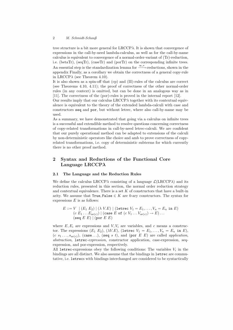
The reduction rules in figure 1 are defined more liberally than necessary for thenormal order reduction, in order to permit an easy use as transformations.
Definition 2.2 (Reduction Rules of the Calculus LRCCPλ). The (base)reduction rules for the calculus and language LRCCPλ are defined in figure 1.The union of (llet-in) and (llet-e) is called (llet), the union of (cp-in) and (cp-e)is called (cp), the union of (porlT), (porrT), (porlF), (porrF) is called (por),and the union of (llet), (lapp), (lseq), (lcase), (lporl) and (lporr) is called (lll).Reductions (and transformations) are denoted using an arrow with super and/orsubscripts: e.g. llet−−→. To explicitly state the context in which a particular reduc-tion is executed we annotate the reduction arrow with the context in which thereduction takes place. If no confusion arises, we omit the context at the arrow.The redex of a reduction is the term as given on the left side of a reduction rule.Transitive closure of reductions is denoted by a +, reflexive transitive closure bya ∗. E.g. ∗−→ is the reflexive, transitive closure of →.

4 M. Schmidt-Schauß
(lbeta) ((λx.s) r) → (letrec x = r in s)(cp-in) (letrec x = s,Env in C[x]) → (letrec x = s,Env in C[s])
where s is an abstraction or a variable or a cv-expression(cp-e) (letrec x = s,Env , y = C[x] in r) → (letrec x = s,Env , y = C[s] in r)
where s is an abstraction or a variable(case) (case (c s1 . . . sn) of . . . (c x1 . . . xn) → t . . .)
→ (letrec x1 = s1, . . . , xn = sn in t)(abs) (letrec x = (c s1 . . . sn),Env in t) →
(letrec x = (c x1 . . . xn), x1 = s1, . . . , xn = sn,Env in t)if (c s1 . . . sn) is not a cv-expression
(seq) (seq s t) → t if s is a value(porlT) (por True t) → True
(porrT) (por t True) → True
(porlF) (por False t) → t(porrF) (por t False) → t(llet-in) (letrec Env1 in (letrec Env2 in r))
→ (letrec Env1,Env2 in r)(llet-e) (letrec Env1, x = (letrec Env2 in sx) in r)
→ (letrec Env1,Env2, x = sx in r)(lapp) ((letrec Env in t) s) → (letrec Env in (t s))(lseq) (seq (letrec Env in s) t) → (letrec Env in (seq s t))(lporl) (por (letrec Env in s) t) → (letrec Env in (por s t))(lporr) (por s (letrec Env in t)) → (letrec Env in (por s t))(lcase) (case (letrec Env in s) of alts) → (letrec Env in (case s of alts))
Fig. 1. Reduction Rules for Call-By-Need
A cv-expression is a constructor-application of the form (c x1 . . . xn), where allxi are variables.
2.2 The Unwind Algorithm
The following labeling algorithm (unwind) will detect the position to which areduction rule will be applied according to normal order. It uses three labels:S, T, V , where T means reduction of the top term, S means reduction of a sub-term, and V labels already visited subexpressions, and S ∨ T matches T as wellas S. The algorithm does not look into S-labeled letrec-expressions. We alsodenote the fresh V only in the result of the unwind-steps, and do not indicatethe already existing V -labels. For a term s the labeling algorithm starts withsT , where no subexpression in s is labeled. The rules of the labeling algorithm
Correctness of Copy in Calculi with Letrec and Por 5
are:
(letrec Env in t)T → (letrec Env in tS)V
(s t)S∨T → (sS t)V
(seq s t)S∨T → (seq sS t)V
(por s t)S∨T → (por sS t)V (non-deterministically)(por s t)S∨T → (por s tS)V (non-deterministically)(case s of alts)S∨T → (case sS of alts)V
(letrec x = s,Env in C[xS ]) → (letrec x = sS ,Env in C[xV ])if s was not labeled
(letrec x = s, y = C[xS ],Env in t)→ (letrec x = sS , y = C[xV ],Env in t)if s was not labeled and if C[x] 6= x
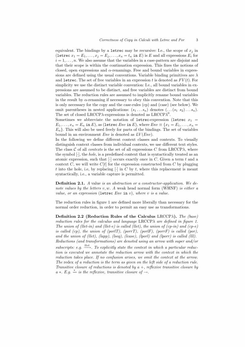
If unwind tries to label an already labelled subterm, then it fails. Otherwise,and if no more rule is applicable, it succeeds. In any case, unwind terminates.For example for (letrec x = x in x)T it will stop with (letrec x = xS in xV )V .Note that the final labelling in case of success is not unique due to the por-rules.
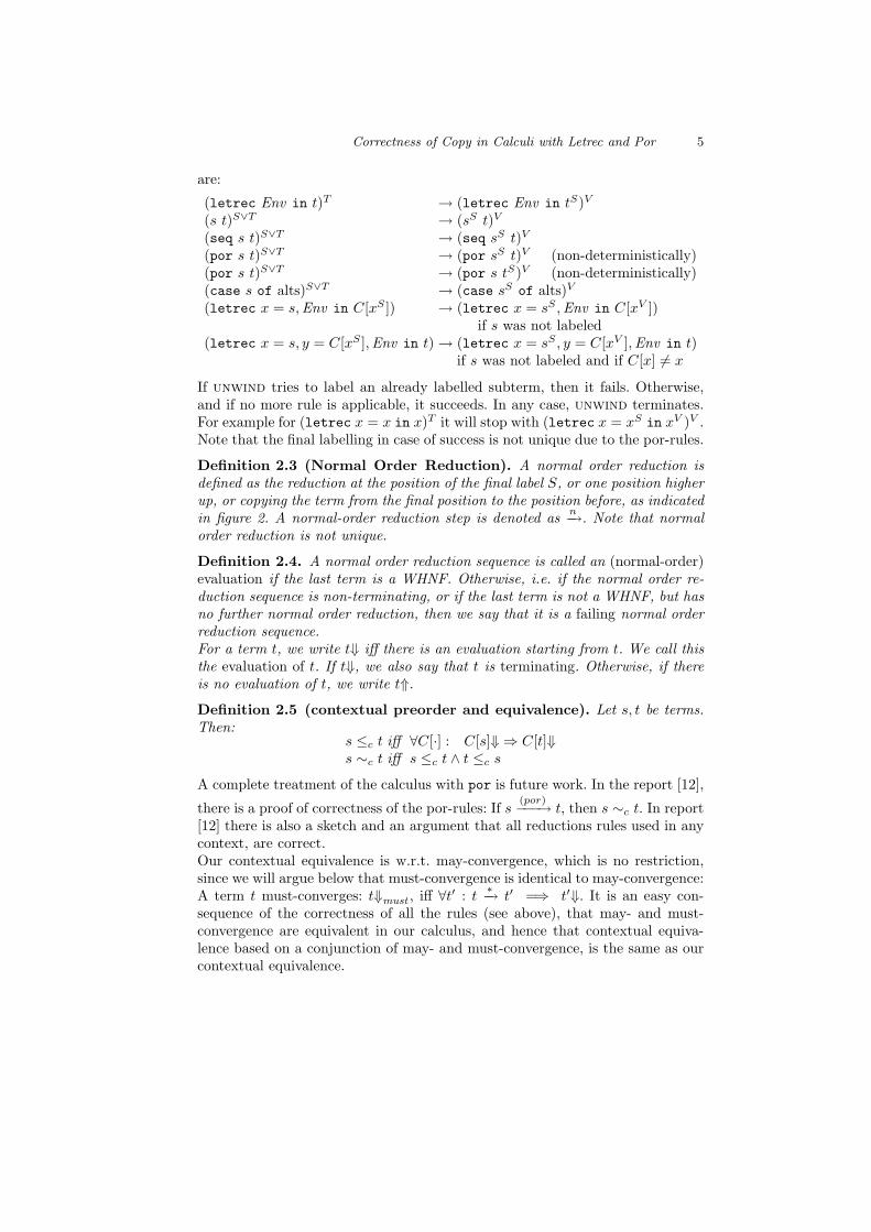
Definition 2.3 (Normal Order Reduction). A normal order reduction isdefined as the reduction at the position of the final label S, or one position higherup, or copying the term from the final position to the position before, as indicatedin figure 2. A normal-order reduction step is denoted as n−→. Note that normalorder reduction is not unique.
Definition 2.4. A normal order reduction sequence is called an (normal-order)evaluation if the last term is a WHNF. Otherwise, i.e. if the normal order re-duction sequence is non-terminating, or if the last term is not a WHNF, but hasno further normal order reduction, then we say that it is a failing normal orderreduction sequence.For a term t, we write t⇓ iff there is an evaluation starting from t. We call thisthe evaluation of t. If t⇓, we also say that t is terminating. Otherwise, if thereis no evaluation of t, we write t⇑.
Definition 2.5 (contextual preorder and equivalence). Let s, t be terms.Then:
s ≤c t iff ∀C[·] : C[s]⇓ ⇒ C[t]⇓s ∼c t iff s ≤c t ∧ t ≤c s
A complete treatment of the calculus with por is future work. In the report [12],
there is a proof of correctness of the por-rules: If s(por)−−−→ t, then s ∼c t. In report
[12] there is also a sketch and an argument that all reductions rules used in anycontext, are correct.Our contextual equivalence is w.r.t. may-convergence, which is no restriction,since we will argue below that must-convergence is identical to may-convergence:A term t must-converges: t⇓must , iff ∀t′ : t
∗−→ t′ =⇒ t′⇓. It is an easy con-sequence of the correctness of all the rules (see above), that may- and must-convergence are equivalent in our calculus, and hence that contextual equiva-lence based on a conjunction of may- and must-convergence, is the same as ourcontextual equivalence.
6 M. Schmidt-Schauß
(lbeta) C[((λx.s)S r)] → C[(letrec x = r in s)](cp-in) (letrec x = sS ,Env in C[xV ]) → (letrec x = s,Env in C[s])
where s is an abstraction or a variable or a cv-expression(cp-e) (letrec x = sS ,Env , y = C[xV ] in r) → (letrec x = s,Env , y = C[s] in r)
where s is an abstraction or a variable or a cv-expression(case) C[(case (c s1 . . . sn)S of . . . (c x1 . . . xn) → t) . . .]
→ C[(letrec x1 = s1, . . . , xn = sn in t)](abs) (letrec x = (c s1 . . . sn)S ,Env in t) →
(letrec x = (c x1 . . . xn), x1 = s1, . . . , xn = sn,Env in t)(seq) C[(seq sS t)] → C[t] if s is a value(porlT) (por TrueS t) → True
(porrT) (por t TrueS) → True
(porlF) (por FalseS t) → t(porrF) (por t FalseS) → t(llet-in) (letrec Env1 in (letrec Env2 in r)S)
→ (letrec Env1,Env2 in r)(llet-e) (letrec Env1, x = (letrec Env2 in sx)S in r)
→ (letrec Env1,Env2, x = sx in r)(lapp) C[((letrec Env in t)S s)] → C[(letrec Env in (t s))](lseq) C[(seq (letrec Env in s)S t)] → C[(letrec Env in (seq s t))](lporl) (por (letrec Env in s)S t) → (letrec Env in (por s t))(lporr) (por s (letrec Env in t)S) → (letrec Env in (por s t))(lcase) C[(case (letrec Env in s)S of alts)] → C[(letrec Env in (case s of alts))]
Fig. 2. Normal-Order Reduction Rules
3 Reductions on Trees
In the following we use “expression” for finite expressions including letrec, and“tree” for the finite or infinite trees, which can co-inductively be defined likeLRλ-expressions, but do not contain letrec-expressions.The infinite tree corresponding to an expression is intended to be the letrec-unfolding of the expression with the extra condition that cyclic variable chainslead to local nontermination, represented by the symbol ⊥. This corresponds tothe infinite trees in the 111-variant of the calculus in [5]. A rigorous definitionis as follows, where we use the explicit binary application operator @, since it iseasier to explain, but stick to the common notation in examples.
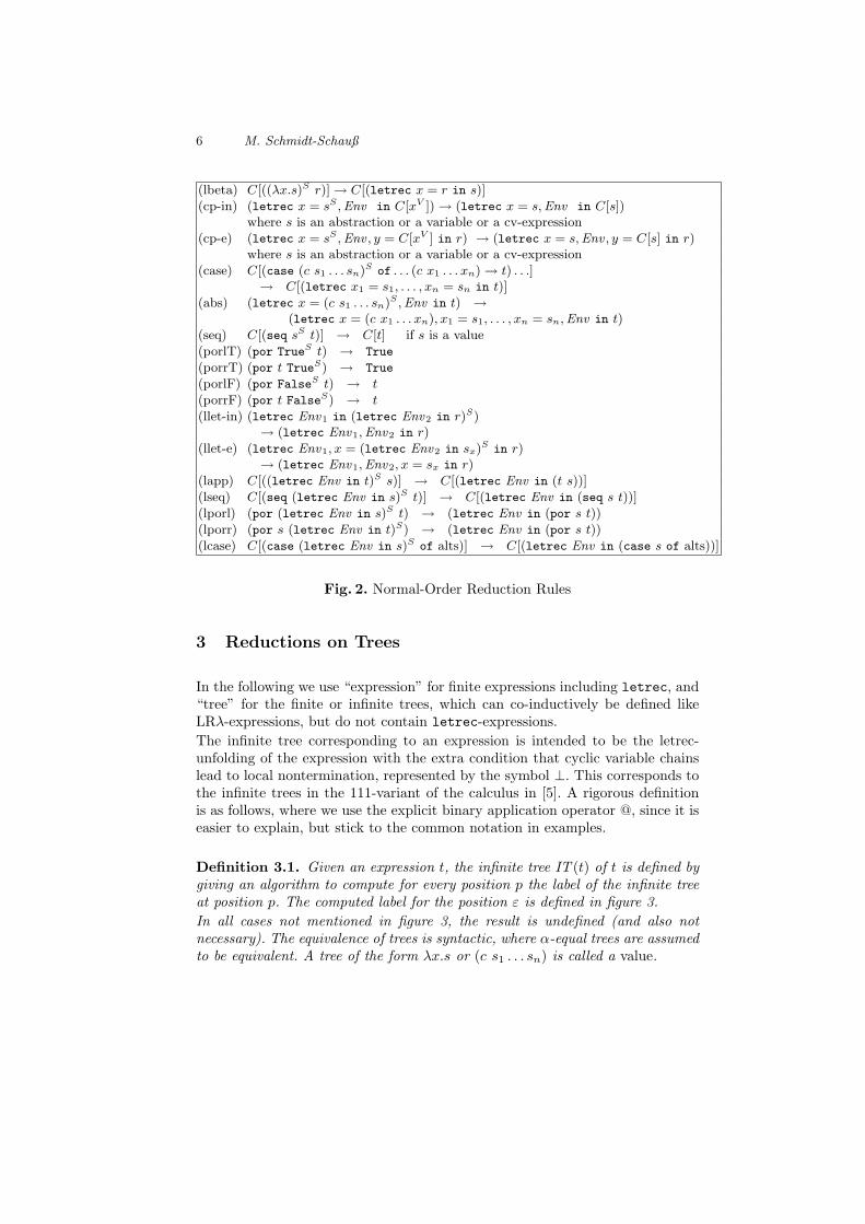
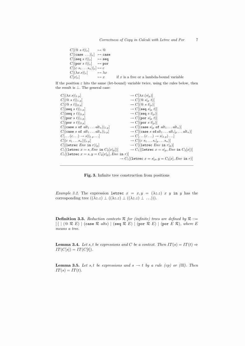
Definition 3.1. Given an expression t, the infinite tree IT (t) of t is defined bygiving an algorithm to compute for every position p the label of the infinite treeat position p. The computed label for the position ε is defined in figure 3.In all cases not mentioned in figure 3, the result is undefined (and also notnecessary). The equivalence of trees is syntactic, where α-equal trees are assumedto be equivalent. A tree of the form λx.s or (c s1 . . . sn) is called a value.
Correctness of Copy in Calculi with Letrec and Por 7
C[(@ s t)|ε] 7→ @C[(case . . .)|ε] 7→ case
C[(seq s t)|ε] 7→ seq
C[(por s t)|ε] 7→ por
C[(c s1 . . . sn)|ε] 7→ cC[(λx.s)|ε] 7→ λxC[x|ε] 7→ x if x is a free or a lambda-bound variable
If the position ε hits the same (let-bound) variable twice, using the rules below, thenthe result is ⊥. The general case:
C[(λx.s)|1.p] → C[λx.(s|p)]C[(@ s t)|1.p] → C[(@ s|p t)]C[(@ s t)|2.p] → C[(@ s t|p)]C[(seq s t)|1.p] → C[(seq s|p t)]C[(seq s t)|2.p] → C[(seq s t|p)]C[(por s t)|1.p] → C[(por s|p t)]C[(por s t)|2.p] → C[(por s t|p)]C[(case s of alt1 . . . altn)|1.p] → C[(case s|p of alt1 . . . altn)]C[(case s of alt1 . . . altn)|i.p] → C[(case s ofalt1 . . . alt i|p . . . altn)]C[. . . (c . . .) → s)|1.p . . .] → C[. . . (c . . .) → s|1.p) . . .]C[(c s1 . . . sn))|i.p] → C[(c s1 . . . si|p . . . sn)]C[(letrec Env in r)|p] → C[(letrec Env in r|p)]C1[(letrec x = s,Env in C2[x|p])] → C1[(letrec x = s|p,Env in C2[x])]C1[(letrec x = s, y = C2[x|p],Env in r)]
→ C1[(letrec x = s|p, y = C2[x],Env in r)]
Fig. 3. Infinite tree construction from positions
Example 3.2. The expression letrec x = x, y = (λz.z) x y in y has thecorresponding tree ((λz.z) ⊥ ((λz.z) ⊥ ((λz.z) ⊥ . . .))).
Definition 3.3. Reduction contexts R for (infinite) trees are defined by R ::=[·] | (@ R E) | (case R alts) | (seq R E) | (por R E) | (por E R), where Emeans a tree.
Lemma 3.4. Let s, t be expressions and C be a context. Then IT (s) = IT (t)⇒IT (C[s]) = IT (C[t]).
Lemma 3.5. Let s, t be expressions and s → t by a rule (cp) or (lll). ThenIT (s) = IT (t).
8 M. Schmidt-Schauß
Definition 3.6. The reduction rules on trees are allowed in any tree contextand are as follows:
(betaTr) ((λx.s) r)→ s[r/x](seqTr) (seq s t) → t if s is a value(caseTr) (case (c s1 . . . sn) of . . . (c x1 . . . xn)→ s . . .) → s[s1/x1, . . . , sn/xn](porlTr) (por True t) → True(porrTr) (por t True) → True(porlFTr) (por False t) → t(porrFTr) (por t False) → t
Let (porTr) be the union of the rules (porlTr), (porrTr), (porlFTr), (porrFTr).If a tree-reduction rule is applied within an R-context, we call it an R-reductionon trees. The redex is the corresponding expression that is reduced in one of therules above. A sequence of R-reductions of T that terminates with a value treeis called evaluation. If T has an evaluation, then we also say T converges anddenote this as T⇓. Note that the R-reduction is not unique.
The (betaTr) as a reduction may modify infinitely many positions, since theremay be infinitely many positions of the variable x. E.g. a top-level (betaTr) ofIT ((λx.(letrec z = (z x) in z)) r) = (λx.((. . . (. . . x) x) x)) r modifies theinfinite number of occurrences of x. Further note that (betaTr) does not overlapwith itself, where we ignore overlaps within the meta-variables s, r.
Lemma 3.7. Let C[(por s t)] be a tree. If different rules can be applied to thepor-expression, then the result is identical. This means that (porTr) is determin-istic as a reduction rule.
Proof. The different possibilities are the Boolean combinations of the arguments:(por True True) results in True; (por False False), (por True False) and(por False True) result in False.
The non-determinism inherent in the R-reduction is only due to reduction atindependent positions within different arguments of a por-expression.
Lemma 3.8. Let s be an expression and let IT (s) be a value tree. Then s⇓.
We will use a variant of infinite outside-in developments [2,5] as a reduction ontrees that may reduce infinitely many redexes in one step. For a more detaileddefinition, in particular concerning the labeling, see [9].
Definition 3.9. For trees S, T , we define the reduction S∞,a−−→ T as follows.
We mark a possibly infinite subset of all a-redexes in S for one reduction typea ∈ {(betaTr), (caseTr), (seqTr), (porTr)}, say with a †. The reduction constructsa new infinite tree top-down by iteratedly using labelled reduction, where the labelof the redex is removed before the reduction. If the reduction does not terminatefor a subtree at the top level of the subtree, then this subtree is the constant ⊥in the result. This recursively defines the result tree top-down.

Correctness of Copy in Calculi with Letrec and Por 9
Sometimes we omit the reduction rule type a, if it is not important, and writeonly ∞−→. We write T⇓(∞) if T
∞,∗−−→ T ′, where T ′ is a value tree.
The reduction S∀,∞,a−−−−→ T is defined as the specific S
∞−→ T -reduction, if alla-redexes in S are labeled.
Note that even for a tree with only two marked redexes, it is possible that afterthe first reduction, infinitely many redexes are labeled.
Example 3.10. We give two examples for a ∞−→-reduction:
– t = (λz.letrec y = λu.u, x = (z (y y) x) in x). The infinite tree IT (t) islike an infinite list, descending to the right, with elements ((λu.u) λu.u). The∞-reduction may label any subset of these redexes, even infinitely many, andthen reduce them by (betaTr).
– t = (letrec x = λy.x (λu.u) in x) has the infinite tree(λy.(λy.(λy. . . .) (λu.u) (λu.u)) (λu.u)) which, depending on the labeling,may reduce to itself, or, if all redexes are labeled, it will reduce to ⊥, i.e.,t∀,∞−−−→ ⊥.
Lemma 3.11. For all trees S, R, T and reduction types a: if S∞,a−−→ R where
the set of a-redex positions is MR, and S∞,a−−→ T , where the the set of a-redex
positions is MS, and MS ⊆ MR, then also T∞,a−−→ R. A special case is that
S∀,∞,a−−−−→ R, and S
∞,a−−→ T imply that T∞,a−−→ R.
S
MR,∞,a
��
MS ,∞,a // T
∞,axxp p p p p p p S
∀,∞,a
��
∞,a // T
∞,axxp p p p p p p
R R
Proof. The argument is that we can mark the a-redexes in S that are not reducedin S
MS ,∞,a−−−−−→ T . Reduce all MR-labeled redexes in the reduction T∞,a−−→ R.
In the appendix it is shown:
Theorem 3.12 (Standardization for tree-reduction). Let S be a tree.Then S⇓(∞) implies S⇓.
4 Properties of Call-by-Need Convergence
4.1 Call-by-Need Convergence Implies Infinite Tree Convergence
Lemma 4.1. If sa−→ t for two expressions s, t and a ∈
{(lbeta), (seq), (case), (por)} then IT (s)∞,a′
−−−→ IT (t) for the tree reductiontype a′ corresponding to a.
Proof. We label every redex of IT (t) that is derived from the redex of sa−→ t.
This is obvious for a por-redex.
Proposition 4.2. Let t be an expression. Then t⇓ ⇒ IT (t)⇓.

10 M. Schmidt-Schauß
4.2 Infinite Tree Convergence Implies Call-by-Need Convergence
Now we show the harder part of the desired equivalence in a series of lemmas.
Lemma 4.3. For every reduction possibility S1R←− T
∞−→ S2, either S1∞−→ S2
or there is some T ′ with S1∞−→ T ′ R←− S2. I.e. we have the following forking
diagrams for trees between an R-reduction and an ∞−→-reduction:
T∞ //
R��
S2
R����� T
∞ //
R��
S2
S1∞ //___ T ′ S1
∞
>>}}
}}
Proof. This follows by checking the overlaps of ∞−→ with R-reductions. Note thatif the type of the ∞−→ and R−→ reductions are different, then the first diagramapplies.
Lemma 4.4. Let T be a tree such that there is an R-evaluation of length n, andlet S be a tree with T
∞−→ S. Then S has an R-evaluation of length ≤ n.
Proof. Follows from Lemma 4.3 by induction.
Lemma 4.5. Let t be a term and let T := IT (t) a′
−→ T ′ be an R-reductionwith a′ ∈ {(betaTr), (seqTr), (caseTr), (porTr)} Then there is an expression t′, areduction t
n,∗−−→ t′ using (lll), (cp) and (abs)-reductions, an expression t′′ witht′
n,a−−→ t′′, where a is the expression reduction corresponding to a, such that there
is a reduction T ′ ∞,a′
−−−→ IT (t′′).
tIT(·) //
n,(cp)∨(lll)∨(abs),∗����� T
R,a′
��∞,a′
ww
Q O L G4�
wro
t′
IT(·)77nnnnnnnn
n,a
����� T ′
∞,a′
�����
t′′IT(·) //______ IT (t′′)
Proof. The expressions t′, t′′ are constructed as follows: t′ is the resulting termfrom a maximal normal-order reduction of t consisting only of (cp), (lll) and
(abs)-reductions. It is clear that such a sequence of(cp)∨(lll)∨(abs),n−−−−−−−−−−−→-reductions
is terminating. Then IT (t) = IT (t′) by Lemma 3.5. The unique normal-order
(a)-redex in t′ must correspond to TR,a′
−−−→ T ′ and is used for the reductiont′
n,a−−→ t′′. Note that the (a)-redex in t′ may correspond to infinitely many
redexes in T . Lemma 4.1 shows that there is a reduction T∞,a′
−−−→ IT (t′′), and
Lemma 3.11 shows that also T ′ ∞,a′
−−−→ IT (t′′).

Correctness of Copy in Calculi with Letrec and Por 11
Proposition 4.6. Let t be an expression such that IT (t)⇓. Then t⇓.
Proof. The precondition IT (t)⇓ and the Standardization Theorem 3.12 implythat there is an R-evaluation of T to a value tree. The base case, where no R-
reductions are necessary is treated in Lemma 3.8. In the general case, let Ta′
−→ T ′
be the unique first R-reduction of a single redex. Lemma 4.5 shows that there
are expressions t′, t′′ with tn,(cp)∨(lll)∨(abs),∗−−−−−−−−−−−−−→ t′
n,lbeta−−−−→ t′′, and T ′ ∞−→ IT (t′′).Lemma 4.4 shows that the number of R-reductions of IT (t′′) to a value treeis strictly smaller than the number of R-reductions of T to a value. Hence wecan use induction on this length and obtain a normal-order reduction of t to aWHNF.
Convergence is equivalent for a term and its corresponding infinite tree:
Theorem 4.7. Let t be an expression. Then t⇓ iff IT (t)⇓.
Proof. This follows from Propositions 4.2 and 4.6.
Definition 4.8. Let the generalized copy rule be:(gcp) C1[letrec x = r . . . C2[x] . . .]→ C1[letrec x = r . . . C2[r] . . .]
This is just like the rule (cp), but all kinds of terms r can be copied, not onlyabstractions. Obviously the following holds:
Lemma 4.9. If sgcp−−→ t, then IT (s) = IT (t)
Theorem 4.10. Let s, t be expressions with sgcp−−→ t Then s ∼c t.
Proof. Lemma 3.4 shows that it is sufficient to show equivalence of terminationof s, t. Lemma 4.9 implies IT (s) = IT (t). Hence equivalence of terminationfollows from Theorem 4.7.
Theorem 4.11. Let s, t be expressions with slll−→ t or s
abs−−→ t Then s ∼c t.
Proof. Follows in the same way as in the proof of Theorem 4.10 using Lemma3.5.
5 Relation Between Call-By-Name and Call-By-Need
For the same language we now treat a call-by-name variant of the reductionstrategy using beta-reduction instead of the rule (lbeta) that respects sharing,and also a substituting case as well as a different (cp) and omitting the (abs)-rule.
12 M. Schmidt-Schauß
Definition 5.1. The call-by-name normal-order reduction is defined by usingthe (lll)-rules and the (seq)-rule and the following modified rules in the call-by-need normal-order reduction as follows:
(beta) ((λx.s)S r)→ s[r/x](cpn-in) (letrec x = sS ,Env in C[xV ])→ (letrec x = s,Env in C[s])
where s is an abstraction or a variableor a constructor-application
(cpn-e) (letrec x = sS ,Env , y = C[xV ] in r)→ (letrec x = s,Env , y = C[s] in r)
where s is an abstraction or a variableor a constructor-application
(casen) (case (c s1 . . . sn)S of . . . (c x1 . . . xn)→ t) . . .→ s[s1/x1, . . . , sn/xn]
where the same labelling and redex is used. Let (cpn) be the union of (cpn-e)and (cpn-in). We denote the reduction as name−−−→, the corresponding call-by-nameconvergence of a term t as t⇓(name), and the corresponding contextual preorderand equivalence as ≤c,name and ∼c,name , respectively.
5.1 Call-by-Name Convergence Implies Infinite Tree Convergence
Lemma 5.2. Let a ∈ {(beta), (casen)}, and a′ ∈ {(betaTr), (caseTr)} be the
corresponding tree-reduction. If sa−→ t for two expressions s, t, then IT (s)
∞,a′
−−−→IT (t).
Proposition 5.3. Let t be an expression. Then t⇓(name)⇒ IT (t)⇓.
Proof. This follows from Lemma 5.2 by induction on the length of the call-by-name evaluation of t, from Lemma 3.5 using the standardization theorem 3.12and from the fact that a WHNF has a value tree as corresponding infinite tree.
5.2 Infinite Tree Convergence Implies Call-by-Name Convergence
Now we show the desired implication also for call-by-name.
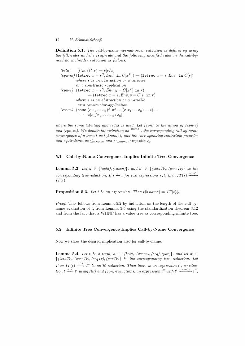
Lemma 5.4. Let t be a term, a ∈ {(beta), (casen), (seq), (por)}, and let a′ ∈{(betaTr), (caseTr), (seqTr), (porTr)} be the corresponding tree reduction. Let
T := IT (t)(a′)−−→ T ′ be an R-reduction. Then there is an expression t′, a reduc-
tion tn,∗−−→ t′ using (lll) and (cpn)-reductions, an expression t′′ with t′
name,a−−−−−→ t′′,
Correctness of Copy in Calculi with Letrec and Por 13
such that there is a reduction T ′ ∞,a′
−−−→ IT (t′′).
tIT(·) //
n,(cpn)∨(lll),∗����� T
R,a′
��∞,a′
ww
Q O L G4�
wro
t′
IT(·)77nnnnnnnn
name,a
����� T ′
∞,a′
�����
t′′IT(·) //______ IT (t′′)
Proof. The expressions t′, t′′ are constructed as follows: t′ is the resulting termfrom a maximal normal-order reduction consisting only of (cpn) and (lll)-
reductions. It is clear that such a sequence of(cpn)∨(lll),n−−−−−−−−→-reductions is termi-
nating. Then IT (t) = IT (t′) by Lemma 3.5. The unique normal-order (a)-redex
in t′ corresponding to Ta′
−→ T ′ is used for the reduction t′name,a−−−−−→ t′′. Note that
the normal-order a-redex in t′ may correspond to infinitely many a′-redexes in
T . Lemma 5.2 shows that there is a reduction T∞,a′
−−−→ IT (t′′), and Lemma 3.11
shows that also T ′ ∞,a′
−−−→ IT (t′′).
Proposition 5.5. Let t be an expression such that IT (t)⇓. Then t⇓(name).
Proof. The precondition IT (t)⇓ means that there is an R-evaluation of T :=IT (t) to a value tree. The base case, where no R-reductions are necessary
is treated in Lemma 3.8. In the general case, let Ta′
−→ T ′ with a′ ∈{(betaTr), (caseTr), (seqTr), (porTr)} be the unique first R-reduction of a sin-
gle redex. Lemma 5.4 shows that there are expressions t′, t′′ with tn,(cpn)∨(lll),∗−−−−−−−−−→
t′name,a−−−−−→ t′′, and T ′ ∞,a′
−−−→ IT (t′′). Lemma 4.4 shows that the number of R-reductions of IT (t′′) to a value tree is strictly smaller than the number of R-reductions of T to a value. Hence we can use induction on this length and obtaina call-by-name normal-order reduction of t to a WHNF.
Now we can show that call-by-name convergence for a term is equivalent toconvergence of its corresponding infinite tree.
Theorem 5.6. Let t be an expression. Then t⇓(name) iff IT (t)⇓.
Proof. Follows from Propositions 5.3 and 5.5.
The strategies call-by-need and call-by-name are equivalent:
Theorem 5.7. The contextual preorders for call-by-need and call-by-name areequivalent.
Proof. This follows from Theorems 4.7 and 5.6.
14 M. Schmidt-Schauß
6 Conclusion
We demonstrated the proof method via infinite trees by showing correctness ofunrestricted copy-reductions and the equivalence of call-by-name and call-by-need for a deterministic letrec-calculus LRCCPλ with case, constructors, seqand parallel or.For non-deterministic calculi like [6,7,8] we plan to extend the method to showcorrectness of the copy-reduction for deterministic subexpressions, which appearsto be a hard obstacle for other methods.
Acknowledgements
I thank David Sabel for reading and correcting drafts of this paper.
References
1. F. Baader and T. Nipkow. Term Rewriting and All That. Cambridge UniversityPress, 1998.
2. H.P. Barendregt. The Lambda Calculus. Its Syntax and Semantics. North-Holland,Amsterdam, New York, 1984.
3. P. Bjesse, K. Claessen, M. Sheeran, and S. Singh. Lava: Hardware Design inHaskell. In International Conference on Functional Programming, ICFP, pages174–184. ACM, 1998.
4. Koen Claessen, Mary Sheeran, and Satnam Singh. Functional hardware descriptionin Lava, volume Fun of Programming of Cornerstones of Computing, chapter 8.Palgrave, March 2003.
5. R. Kennaway, J. W. Klop, M. R. Sleep, and F.-J. de Vries. Infinitary lambdacalculus. Theor. Comput. Sci, 175(1):93–125, 1997.
6. A. K.D. Moran, D. Sands, and M. Carlsson. Erratic fudgets: A semantic theory foran embedded coordination language. In Coordination ’99, volume 1594 of LNCS,pages 85–102. Springer-Verlag, 1999.
7. A.K.D. Moran. Call-by-name, call-by-need, and McCarthys Amb. PhD thesis,Dept. of Comp. Science, Chalmers University, Sweden, 1998.
8. D. Sabel and M. Schmidt-Schauß. A call-by-need lambda-calculus with locallybottom-avoiding choice: Context lemma and correctness of transformations. Frankreport 24, Inst. Informatik. J.W.G.-university Frankfurt, 2006.
9. M. Schmidt-Schauß. Equivalence of call-by-name and call-by-need for lambda-calculi with letrec. Frank report 25, Inst. Informatik. J.W.G.-university Frankfurt,2006.
10. M. Schmidt-Schauß. Correctness of copy in calculi with letrec, case and construc-tors. Frank report 28, Inst. Informatik. J.W.G.-University Frankfurt, 2007.
11. M. Schmidt-Schauß, M. Schutz, and D. Sabel. A complete proof of the safety ofNocker’s strictness analysis. Frank report 20, Inst. Informatik. J.W.G.-UniversityFrankfurt, 2005.
12. Manfred Schmidt-Schauß and David Sabel. Program transformation for functionalcircuit descriptions. Frank report 30, Institut fur Informatik. Fachbereich Infor-matik und Mathematik. J. W. Goethe-Universitat Frankfurt am Main, 2007.
13. M. Sheeran. Hardware design and functional programming: a perfect match.J.UCS, 11(7):1135–1158, 2005.

Correctness of Copy in Calculi with Letrec and Por 15
A Labeled Reduction
We define two variants of the notion of labeled reduction for trees. Labelledreduction is used to identify correspondences of positions during a reductionstep. It will be used in two variants, the joining variant for the inheritance ofpositions during reductions and the consuming one for a reduction that is similarto a development: Some redexes are marked at the start of the reduction process,and all the labeled redexes have to be reduced.
Definition A.1 (labeled reduction of trees). First we define joining labeledreduction for sets of labels.Let S be a tree and assume there are sets of labels at certain (subexpression-)positions of S. We can assume that every position is labeled, perhaps with an
empty set. Let T be a tree with S(betaTr)−−−−−→ T , and assume that the reduction is
S = C[(λx.r) s]→ C[r[s/x]]. Then the labels in the result are as follows:
– label sets within C are unchanged.– label sets properly within s are copied to all occurrences of s in the result.– If r = x, then ((λx.xA)B sC)D → r[s/x]A∪B∪C∪D.– If r 6= x, label sets of positions properly within r and not at x remain un-
changed.– If r 6= x, the label sets of the new occurrences of sB in C[r[s/x]] are as fol-
lows: For every occurrence of xA in r the new label set of the new occurrenceof s is A ∪B.
– If r 6= x, the new label set of r[s/x] is computed as follows: ((λx.rA)B s)C →r[s/x]A∪B∪C .
In an analogous way the inheritance for the case and seq-rule are defined; wemake only the redex-case explicit:(case (c s1 . . . sn)A of . . . ((c x1 . . . xn) → tB) . . .)C
→ t[s1/x1, . . . , sn/xn]A∪B∪C , where in the case that t is a variablexi, the label of respective si is also joined.(seq sA tB)C → tB∪C if s is a value. Here the label of s is not inherited,since s is discarded after evaluation.
The consuming labeled reduction is like the joining variant, and can be derivedby removing the label of the redex before the reduction and then using the joiningvariant.We will use the consuming labeled reduction below for one label † in the devel-opments. In the case of only one label-value it is usually assumed that emptysets mean no label, and a non-empty set, which must be a singleton in this case,means that the position is labeled.
The labelled reduction in the True-case of por-reductions must be specified, sincethese are the only rules, where on the right hand side a symbol is used where the

16 M. Schmidt-Schauß
predecessor is ambiguous: We assume that the following labelling inheritance isused:
(por TrueA TrueB)C → TrueA∪B∪C
(por TrueA t)C → TrueA∪C if t 6= True(por t TrueB)C → TrueB∪C if t 6= True(por FalseA FalseB)C → FalseC
(por FalseA tB)C → tB∪C
(por tA FalseB)C → tA∪C
B Standardization of Tree Reduction
Definition B.1. We call a set M of positions prefix-closed, iff for every p ∈M ,and prefix q of p, also q ∈M . If M is a finite prefix-closed set of positions of thetree T , and for every p ∈ M , we have T|p 6= ⊥, then we say M is admissible,and call this set an FAPC-set (finite admissible prefixed-closed) of positions ofT .
In the following we use sets of positions in terms.
Lemma B.2. Let S, T be trees with S∞−→ T , and let MT be an FAPC-set of
positions of T . Then the set of positions MS which are mapped by joining labeledreduction to positions in MT is also an FAPC-set of positions of S.
Proof. First we analyze the transport of positions by the reduction S∞−→ T
using joining labeled reduction. For the reduction S∞−→ T , there are some †-
labeled positions in S, which are exactly the redexes that are to be reduced.We determine the new position(s) in T of every position from S. This has to bedone by looking at the construction of the results of the reduction as explainedin Definition 3.9. We will use joining labeled reduction to trace the positions.At the start of the construction, we assume that all S-positions are labeledwith a singleton set, containing their position. The definition implies that aftera single (betaTr), (seqTr), (caseTr) or (porTr)-reduction, the set of labels atevery position remains a finite set. If for a subtree A the top-reduction sequencedoes not terminate, then this subtree will be ⊥ in the resulting tree, hence onlyfinitely many reductions for A have to be considered. The construction will thenproceed with the direct subtrees of A, which guarantees that every position inT either has finitely many ancestors in S, or is ⊥. It is obvious that there areno positions in MS pointing to ⊥.Now we can simply reverse the mapping. For the set MT , we define the set MS asthe set of all positions of S that are in the label set of any position in MT . Thisset is finite, since there are no positions of ⊥ in MT , there is also no position of⊥ in MS . The set MS is prefix-closed, since the mapping behaves monotone, i.e.if p is a position in S, q is a prefix of p, then for every position p′ in T that isderived from p, there is a position q′ in T derived from q such that q′ is a prefixof p′.
Correctness of Copy in Calculi with Letrec and Por 17
Lemma B.3. Let S be a tree, and let red be the reduction sequence S = S0∞−→
S1∞−→ S2
∞−→ . . .∞−→ Sn = S′, where S′ is a value. Then the set M0 of all
positions of S that are mapped by red to the top position of S′ is an FAPC-setof S.
Proof. We perform induction on the number of ∞−→-reductions in the sequenceS = S0
∞−→ S1∞−→ S2
∞−→ . . .∞−→ Sn = S′. If the sequence has no reductions,
then the lemma holds, since M = {ε} consists only of the top position of S′. Inthe induction step, we can assume that the lemma holds already for the reductionsequence S1
∞−→ S2∞−→ . . .
∞−→ Sn = S′, and then we can apply Lemma B.2 tothe reduction step S0
∞−→ S1, which shows the Lemma.
Corollary B.4. Let S be a tree, and let red be the reduction sequence S =S0
∞−→ S1∞−→ S2
∞−→ . . .∞−→ Sn = S′, where S′ is a value. If a position p from
S is not mapped by red to the top position of S′, then all positions q of S suchthat p is a prefix of q, are also not mapped to the top position of S′.
We distinguish relevant and irrelevant positions for a reduction sequence to avalue:
Definition B.5. Let red ≡ S∞,∗−−→ S′ be a reduction sequence, where S′ is a
value. Let M0 be the set of positions of S that are mapped using joining labeledreduction to the top position of S′. Then the positions p ∈ M0 in S are calledrelevant for red, and the positions of S that are not in M0 are called irrelevantfor red. We omit red in the notation if it is clear from the context,
Note that the set of relevant positions for some reduction sequence red ≡ S∞,∗−−→
S′ is always an FAPC-set in S.
Let(Tr),∗−−−−→ be the reduction
(betaTr),∗−−−−−−−−→ ∪
(seqTr),∗−−−−−−−→ ∪
(caseTr),∗−−−−−−−→
∪(porTr),∗−−−−−−−→.
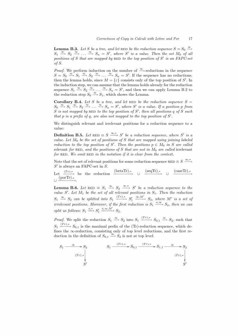
Lemma B.6. Let red ≡ S1∞−→ S2
∞,∗−−→ S′ be a reduction sequence to thevalue S′. Let M1 be the set of all relevant positions in S1. Then the reduction
S1∞−→ S2 can be splitted into S1
(Tr),∗−−−−→ S′1∞,M ′
−−−−→ S2, where M ′ is a set ofirrelevant positions. Moreover, if the first reduction is S1
a,∞−−→ S2, then we can
split as follows: S1a,∗−−→ S′1
a,∞,M ′
−−−−−→ S2.
Proof. We split the reduction S1∞−→ S2 into S1
(Tr),∗−−−−→ S0,1∞−→ S2, such that
S1(Tr),∗−−−−→ S0,1 is the maximal prefix of the (Tr)-reduction sequence, which de-
fines the ∞-reduction, consisting only of top level reductions, and the first re-duction in the definition of S0,1
∞−→ S2 is not at top level.
S1∞ // S2
(Tr),∗
��
S1
(Tr),∗ // S0,1(Tr),∗ // S1,1
∞ // S2
(Tr),∗
��S′ S′

18 M. Schmidt-Schauß
Let M0,1 be the FAPC-set of all positions in S0,1 that are mapped by S0,1∞−→ S2
to M2, the set of relevant positions in S2. By induction on the depth of positionsin M0,1, and since we can split into reduction sequences at independent positions,
it is easy to see that there is a reduction sequence S0,1(Tr),∗−−−−→ S1,1
∞−→ S1, suchthat the reduction S1,1
∞−→ S2 is w.r.t. a set M1,1 of irrelevant positions.
Lemma B.7. Let red = S0M0,∞−−−−→ S1 be a reduction of trees to a value S1,
such that M0 is the set of irrelevant positions in S0. Then S0 is a value
Proof. This is obvious.
Lemma B.8. Let red = S0M0,∞−−−−→ S1
a−→ S2 · red′ for a ∈{(betaTr), (seqTr), (caseTr), (porTr)} be a reduction sequence of trees to a value,such that M0 is the set of irrelevant positions in S0 and let S1
a−→ S2 be a reduc-tion at the relevant position p1.
Then there is some S′0, a set M ′0 of positions of S′0 with S0
a−→ S′0M ′
0,∞−−−−→ S2, such
w.r.t the reduction sequence red′′ ≡ S′0M ′
0,∞−−−−→ S2 ·red′, the set of positions M ′0
is irrelevant. Moreover, the reduction S0a−→ S′0 is also at the relevant position
p1, and the constructed reduction sequence has the same length and reduces atthe same positions.
S0M0,∞ //
a
����� S1
a
��S′0
M ′0,∞ //___ S2
red′
��·
Proof. Let C be a multicontext that has holes at p1, the position of the redexof the S1
a−→ S2-reduction, and additionally finitely many holes, such that allpositions of M0 are below a hole of C. Then the following diagrams shows thegiven and the derived reductions for every type of reduction:
C[s1, . . . , sn, ((λx.s) r)]M0,∞//
(betaTr)
�����
C[s′1, . . . , s′n, ((λx.s′) r′)]
(betaTr)
��C[s1, . . . , sn, s[r/x]]
M ′0,∞ //_____ C[s′1, . . . , s
′n, s′[r′/x]]
For case a similar diagram can be drawn. For seqthe diagram is as follows:
C[s1, . . . , sn, (seq v t)]M0,∞//
(seqTr)
�����
C[s′1, . . . , s′n, (seq v′ t′)]
(seqTr)
��C[s1, . . . , sn, t]
M ′0,∞ //_______ C[s′1, . . . , s
′n, t′]
Correctness of Copy in Calculi with Letrec and Por 19
The diagram shows how to construct the required reduction.
Lemma B.9. Let S be a tree with S⇓(∞). Then there is a finite (perhaps non-
R-) reduction sequence S(Tr),∗−−−−→ T , such that T is a value tree.
Proof. Let red be the ∞-reduction sequence from S to a value tree S′. LemmaB.3 shows that the set of all positions in S that are mapped by red to thetop position of S′ is an FAPC-set. Using Lemma B.6, the reduction sequence
can be splitted into S(Tr),∗−−−−→ S0,1
(Tr),∗−−−−→ S1,1∞−→ S1, such that the reduction
S1,1∞−→ S1 is w.r.t. a set M1,1 of irrelevant positions.
Now induction on the length of the reduction sequence S1(Tr),∗−−−−→ S′ and using
Lemma B.8 shows that the reduction S1,1∞−→ S1 can be shifted to the end of the
reduction sequence until we obtain a reduction sequence S(betaTr),∗−−−−−−−→ S′′, where
S′′ is a value. ut
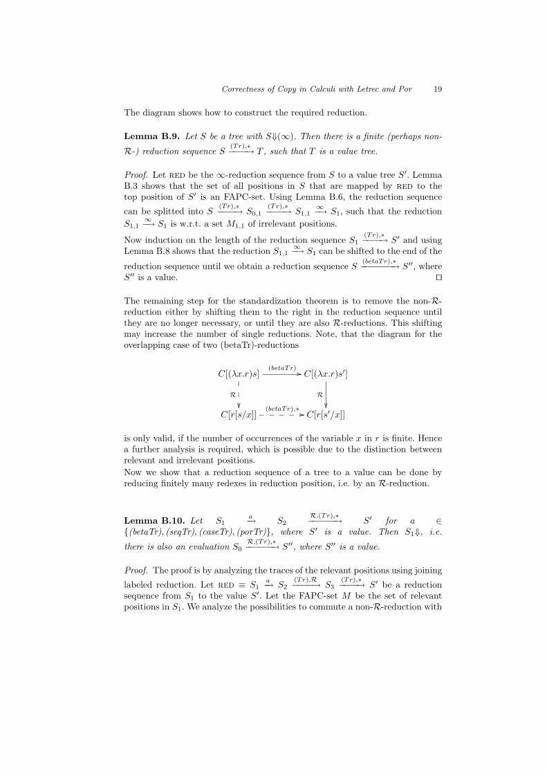
The remaining step for the standardization theorem is to remove the non-R-reduction either by shifting them to the right in the reduction sequence untilthey are no longer necessary, or until they are also R-reductions. This shiftingmay increase the number of single reductions. Note, that the diagram for theoverlapping case of two (betaTr)-reductions
C[(λx.r)s](betaTr) //
R�����
C[(λx.r)s′]
R��
C[r[s/x]](betaTr),∗ //_____ C[r[s′/x]]
is only valid, if the number of occurrences of the variable x in r is finite. Hencea further analysis is required, which is possible due to the distinction betweenrelevant and irrelevant positions.Now we show that a reduction sequence of a tree to a value can be done byreducing finitely many redexes in reduction position, i.e. by an R-reduction.
Lemma B.10. Let S1a−→ S2
R,(Tr),∗−−−−−−→ S′ for a ∈{(betaTr), (seqTr), (caseTr), (porTr)}, where S′ is a value. Then S1⇓, i.e.
there is also an evaluation S0R,(Tr),∗−−−−−−→ S′′, where S′′ is a value.
Proof. The proof is by analyzing the traces of the relevant positions using joining
labeled reduction. Let red ≡ S1a−→ S2
(Tr),R−−−−→ S3(Tr),∗−−−−→ S′ be a reduction
sequence from S1 to the value S′. Let the FAPC-set M be the set of relevantpositions in S1. We analyze the possibilities to commute a non-R-reduction with
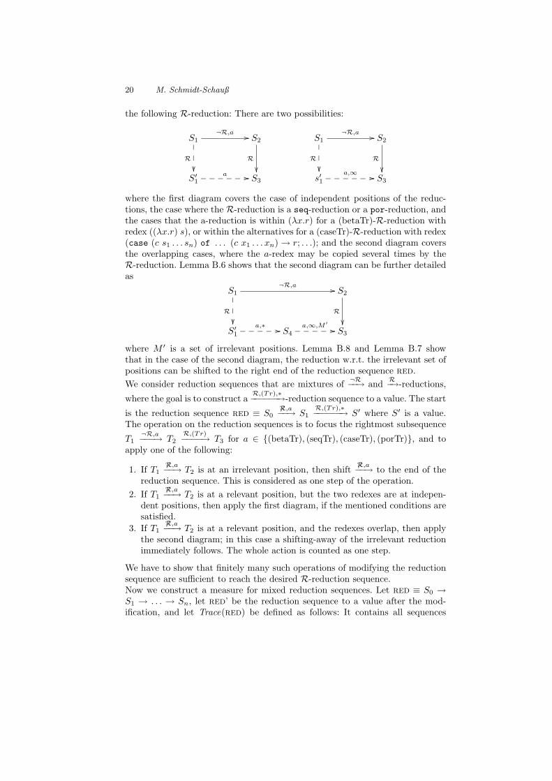
20 M. Schmidt-Schauß
the following R-reduction: There are two possibilities:
S1¬R,a //
R����� S2
R
��
S1¬R,a //
R����� S2
R
��S′1
a //______ S3 s′1a,∞ //______ S3
where the first diagram covers the case of independent positions of the reduc-tions, the case where the R-reduction is a seq-reduction or a por-reduction, andthe cases that the a-reduction is within (λx.r) for a (betaTr)-R-reduction withredex ((λx.r) s), or within the alternatives for a (caseTr)-R-reduction with redex(case (c s1 . . . sn) of . . . (c x1 . . . xn)→ r; . . .); and the second diagram coversthe overlapping cases, where the a-redex may be copied several times by theR-reduction. Lemma B.6 shows that the second diagram can be further detailedas
S1¬R,a //
R����� S2
R
��S′1
a,∗ //_____ S4a,∞,M ′
//_____ S3
where M ′ is a set of irrelevant positions. Lemma B.8 and Lemma B.7 showthat in the case of the second diagram, the reduction w.r.t. the irrelevant set ofpositions can be shifted to the right end of the reduction sequence red.We consider reduction sequences that are mixtures of ¬R−−→ and R−→-reductions,
where the goal is to construct aR,(Tr),∗−−−−−−→-reduction sequence to a value. The start
is the reduction sequence red ≡ S06R,a−−→ S1
R,(Tr),∗−−−−−−→ S′ where S′ is a value.The operation on the reduction sequences is to focus the rightmost subsequence
T1¬R,a−−−→ T2
R,(Tr)−−−−→ T3 for a ∈ {(betaTr), (seqTr), (caseTr), (porTr)}, and toapply one of the following:
1. If T16R,a−−→ T2 is at an irrelevant position, then shift
6R,a−−→ to the end of thereduction sequence. This is considered as one step of the operation.
2. If T16R,a−−→ T2 is at a relevant position, but the two redexes are at indepen-
dent positions, then apply the first diagram, if the mentioned conditions aresatisfied.
3. If T16R,a−−→ T2 is at a relevant position, and the redexes overlap, then apply
the second diagram; in this case a shifting-away of the irrelevant reductionimmediately follows. The whole action is counted as one step.
We have to show that finitely many such operations of modifying the reductionsequence are sufficient to reach the desired R-reduction sequence.Now we construct a measure for mixed reduction sequences. Let red ≡ S0 →S1 → . . . → Sn, let red’ be the reduction sequence to a value after the mod-ification, and let Trace(red) be defined as follows: It contains all sequences
Correctness of Copy in Calculi with Letrec and Por 21
p0, p1, . . . , pn, called traces, where p0 is a red-relevant position of S0, and for alli: pi is a relevant position in Si, and pi+1 is a successor of pi. The trace stops ei-ther at the last term, or at pi, if pi is the position of the R-redex that is reducedin this step, or the position of the term (c s1 . . . sn) in the R-(caseTr)-redex(case (c s1 . . . sn) . . .). An annotated trace is a trace, where the form of inher-itance is also annotated: p
a1−→ p1a2−→ . . . ,
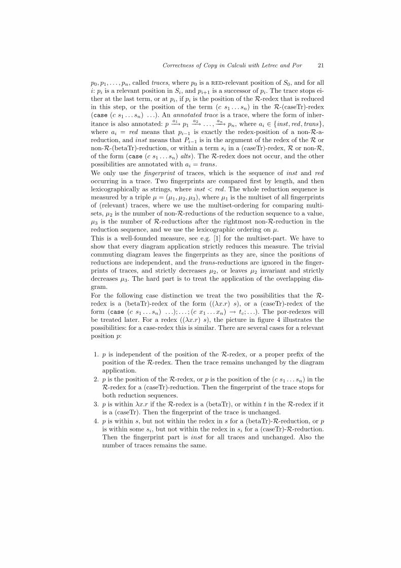
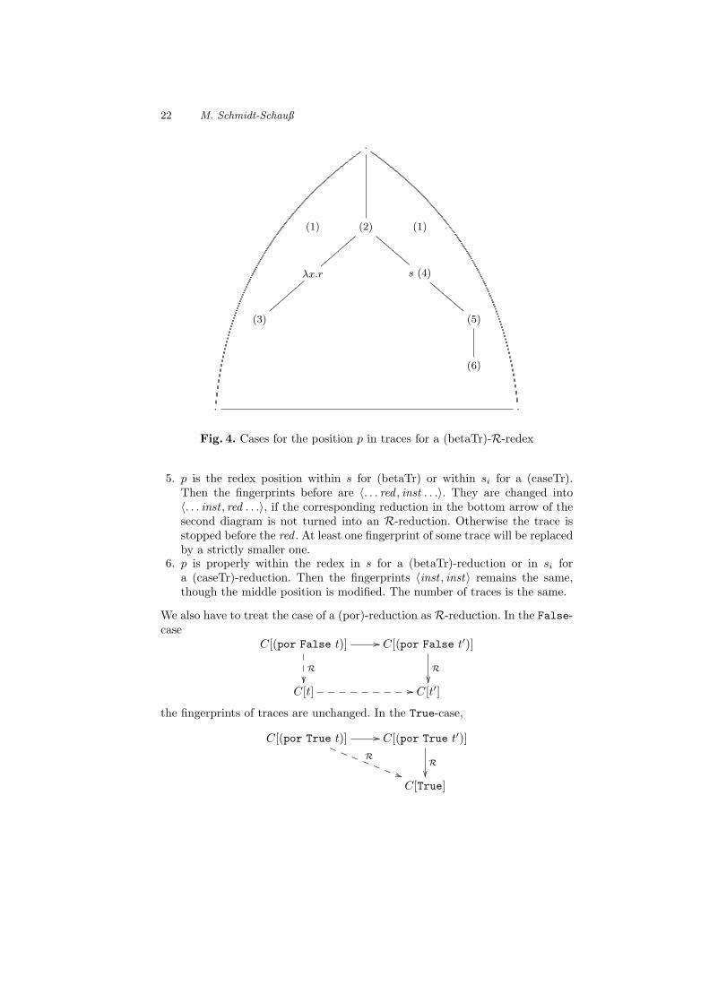
an−−→ pn, where ai ∈ {inst , red , trans},where ai = red means that pi−1 is exactly the redex-position of a non-R-a-reduction, and inst means that Pi−1 is in the argument of the redex of the R ornon-R-(betaTr)-reduction, or within a term si in a (caseTr)-redex, R or non-R,of the form (case (c s1 . . . sn) alts). The R-redex does not occur, and the otherpossibilities are annotated with ai = trans.We only use the fingerprint of traces, which is the sequence of inst and redoccurring in a trace. Two fingerprints are compared first by length, and thenlexicographically as strings, where inst < red . The whole reduction sequence ismeasured by a triple µ = (µ1, µ2, µ3), where µ1 is the multiset of all fingerprintsof (relevant) traces, where we use the multiset-ordering for comparing multi-sets, µ2 is the number of non-R-reductions of the reduction sequence to a value,µ3 is the number of R-reductions after the rightmost non-R-reduction in thereduction sequence, and we use the lexicographic ordering on µ.This is a well-founded measure, see e.g. [1] for the multiset-part. We have toshow that every diagram application strictly reduces this measure. The trivialcommuting diagram leaves the fingerprints as they are, since the positions ofreductions are independent, and the trans-reductions are ignored in the finger-prints of traces, and strictly decreases µ2, or leaves µ2 invariant and strictlydecreases µ3. The hard part is to treat the application of the overlapping dia-gram.For the following case distinction we treat the two possibilities that the R-redex is a (betaTr)-redex of the form ((λx.r) s), or a (caseTr)-redex of theform (case (c s1 . . . sn) . . .); . . . ; (c x1 . . . xn) → tc; . . .). The por-redexes willbe treated later. For a redex ((λx.r) s), the picture in figure 4 illustrates thepossibilities: for a case-redex this is similar. There are several cases for a relevantposition p:
1. p is independent of the position of the R-redex, or a proper prefix of theposition of the R-redex. Then the trace remains unchanged by the diagramapplication.
2. p is the position of the R-redex, or p is the position of the (c s1 . . . sn) in theR-redex for a (caseTr)-reduction. Then the fingerprint of the trace stops forboth reduction sequences.
3. p is within λx.r if the R-redex is a (betaTr), or within t in the R-redex if itis a (caseTr). Then the fingerprint of the trace is unchanged.
4. p is within s, but not within the redex in s for a (betaTr)-R-reduction, or pis within some si, but not within the redex in si for a (caseTr)-R-reduction.Then the fingerprint part is inst for all traces and unchanged. Also thenumber of traces remains the same.
22 M. Schmidt-Schauß
·
(1) (2)
{{{{
{{{{
DDDD
DDDD
(1)
λx.r
{{{{
{{{{
s (4)
DDDD
DDDD
(3) (5)
(6)
· ·
Fig. 4. Cases for the position p in traces for a (betaTr)-R-redex
5. p is the redex position within s for (betaTr) or within si for a (caseTr).Then the fingerprints before are 〈. . . red , inst . . .〉. They are changed into〈. . . inst , red . . .〉, if the corresponding reduction in the bottom arrow of thesecond diagram is not turned into an R-reduction. Otherwise the trace isstopped before the red . At least one fingerprint of some trace will be replacedby a strictly smaller one.
6. p is properly within the redex in s for a (betaTr)-reduction or in si fora (caseTr)-reduction. Then the fingerprints 〈inst , inst〉 remains the same,though the middle position is modified. The number of traces is the same.
We also have to treat the case of a (por)-reduction as R-reduction. In the False-case
C[(por False t)] //
R�����
C[(por False t′)]
R��
C[t] //_________ C[t′]
the fingerprints of traces are unchanged. In the True-case,
C[(por True t)] //
R
))RRRRRRRC[(por True t′)]
R��
C[True]
Correctness of Copy in Calculi with Letrec and Por 23
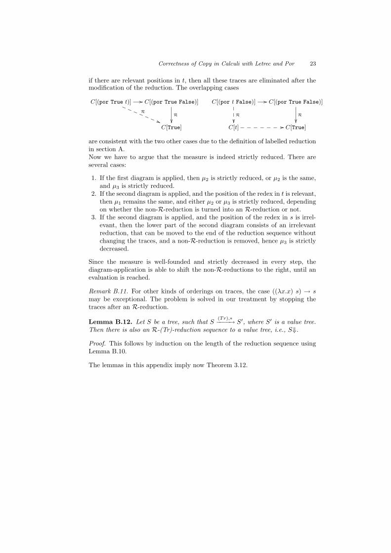
if there are relevant positions in t, then all these traces are eliminated after themodification of the reduction. The overlapping cases
C[(por True t)] //
R
((RRRRRRRC[(por True False)]
R��
C[(por t False)] //
R�����
C[(por True False)]
R��
C[True] C[t] //_______ C[True]
are consistent with the two other cases due to the definition of labelled reductionin section A.Now we have to argue that the measure is indeed strictly reduced. There areseveral cases:
1. If the first diagram is applied, then µ2 is strictly reduced, or µ2 is the same,and µ3 is strictly reduced.
2. If the second diagram is applied, and the position of the redex in t is relevant,then µ1 remains the same, and either µ2 or µ3 is strictly reduced, dependingon whether the non-R-reduction is turned into an R-reduction or not.
3. If the second diagram is applied, and the position of the redex in s is irrel-evant, then the lower part of the second diagram consists of an irrelevantreduction, that can be moved to the end of the reduction sequence withoutchanging the traces, and a non-R-reduction is removed, hence µ3 is strictlydecreased.
Since the measure is well-founded and strictly decreased in every step, thediagram-application is able to shift the non-R-reductions to the right, until anevaluation is reached.
Remark B.11. For other kinds of orderings on traces, the case ((λx.x) s) → smay be exceptional. The problem is solved in our treatment by stopping thetraces after an R-reduction.
Lemma B.12. Let S be a tree, such that S(Tr),∗−−−−→ S′, where S′ is a value tree.
Then there is also an R-(Tr)-reduction sequence to a value tree, i.e., S⇓.
Proof. This follows by induction on the length of the reduction sequence usingLemma B.10.
The lemmas in this appendix imply now Theorem 3.12.