data-augmented modeling of intracranial pressure
TRANSCRIPT

Data-augmented modeling of intracranial pressure
Jian-Xun Wang∗1,2, Xiao Hu†3, and Shawn C. Shadden‡1
1Mechanical Engineering, University of California, Berkeley, CA
2Aerospace and Mechanical Engineering, Center of Informatics and Computational Science,
University of Notre Dame, Notre Dame, IN
3Department of Physiological Nursing, Department of Neurological surgery, Institute of
Computational Health Sciences, UCSF Joint Bio-Engineering Graduate Program, University of
California, San Francisco, CA
abbreviated title: Data-augmented modeling of ICP
correspondence: Jian-Xun Wang, Aerospace and Mechanical Engineering, Center of
Informatics and Computational Science, University of Notre Dame, Notre Dame, IN,
USA. e-mail: [email protected]
Abstract
Precise management of patients with cerebral diseases often requires intracra-
nial pressure (ICP) monitoring, which is highly invasive and requires a specialized
ICU setting. The ability to noninvasively estimate ICP is highly compelling as an al-
ternative to, or screening for, invasive ICP measurement. Most existing approaches
for noninvasive ICP estimation aim to build a regression function that maps noninva-
sive measurements to an ICP estimate using statistical learning techniques. These
∗Email address: [email protected]†Email address: [email protected]‡Email address: [email protected]
1
arX
iv:1
807.
1034
5v2
[ph
ysic
s.m
ed-p
h] 1
8 D
ec 2
018

data-based approaches have met limited success, likely because the amount of train-
ing data needed is onerous for this complex applications. In this work, we discuss
an alternative strategy that aims to better utilize noninvasive measurement data by
leveraging mechanistic understanding of physiology. Specifically, we developed a
Bayesian framework that combines a multiscale model of intracranial physiology with
noninvasive measurements of cerebral blood flow using transcranial Doppler. Virtual
experiments with synthetic data are conducted to verify and analyze the proposed
framework. A preliminary clinical application study on two patients is also performed
in which we demonstrate the ability of this method to improve ICP prediction.
keywords: cerebrovascular dynamics; data assimilation; patient-specific modeling;
transcranial Doppler.
2

1 Introduction
Determination of intracranial pressure (ICP) is essential for precise management of pa-
tients with brain injury, hemorrhage, tumor, hydrocephalus and other neurologic condi-
tions1. Elevated ICP reduces cerebral blood flow, which can lead to brain damage or
death10. The clinical standard for ICP monitoring, which entails penetrations of the skull
and brain, carries the risks of hemorrhage, infection and tissue damage12. Moreover,
such invasive techniques require neurosurgical expertise and a specialized ICU setting44.
Even in such a setting, a significant concern is to identify when ICP monitoring should
be initiated for a given patient. A noninvasive method to estimate ICP can reduce the
risks of invasive ICP monitoring, better identify patients needing invasive monitoring, and
potentially broaden ICP evaluation beyond the ICU setting.
The majority of noninvasive ICP (nICP) research has been to identify noninvasive sig-
nals that are correlated to ICP. These have included pupil size, intraocular pressure, optic
nerve sheath diameter, tympanic membrane displacement, cerebral blood flow velocity
(CBFV), visual evoked potentials and skull movements, among others4. However, iden-
tifying noninvasive signals that are correlated to ICP often only enables inference of ICP
trending or its detrimental effects. There remains a need to quantitatively estimate ICP
from noninvasive signals for proper clinical response44,4. To address this challenge, nICP
research has recently sought to develop algorithmic solutions that can bridge the gap
between noninvasive measurements (measurable states) and ICP (the hidden state)7.
To connect measurable states with a hidden state requires a model, which can be
data-based or theory-based. Most prior works on nICP estimation have been data-based,
and have tried to construct mapping functions between noninvasive signals and ICP us-
ing supervised learning techniques, including linear/nonlinear regression6, support vector
machines (SVM)43, kernel spectral regression24, and artificial neural networks15. Despite
the varied attempts, these methods have struggled to achieve accurate nICP assessment
for a de novo patient. The limitation of a data-based approach is the requirement of suffi-
3

cient training data. Data is inherently limited for this problem because gold-standard ICP
measurement is highly invasive, data can vary in quality or consistency, and complications
with sharing patient data. Moreover, a large amount of data is likely necessary due to the
complexity of the underlying physiology and inter-patient variability.
Utilization of theory-based models may help to alleviate the need for inordinate training
data, and maximize the utility of each individual’s data, when compared to a data-based
approach. Theory-based intracranial modeling has advanced in recent years to increase
our understanding of the mechanisms that drive intracranial pressure42,26. In contrast to
black-box models that depend on training data, theory-based models rely on physiologi-
cal knowledge and physical principles. It is broadly accepted that ICP dynamics is driven
by the interactions between cerebral blood flow (CBF), cerebrospinal fluid (CSF), and
brain soft tissue under the constraints of a rigid skull. Lumped-parameter (LP) models are
widely employed for modeling the dynamics of these intracranial components, and among
the several publications in this area, Ursino et al.41,40, Stevens et al.38, and Linninger et
al.27 have contributed significantly to establishing theoretical models of the component
dynamics. However, the clinical impact of existing theory-based models remains negligi-
ble.
The challenges of using theory-based model for ICP estimation include the coupling
of sufficiently comprehensive component models needed to capture the important phys-
iology, and calibration of these model parameters for a de novo patient. A promising
approach is to combine useful information from both theory-based modeling and nonin-
vasive measurement. Kashif et al.22 demonstrated the merits of this idea. Namely, they
showed that the accuracy of a model-based nICP approach was significantly improved
compared to a purely data-driven approach. Hu et al.14 also exploited using a basic
physiologic model with measured data and filtering to estimate ICP. A recent review7
comprehensively comparing existing nICP algorithms also confirmed the advantage of
introducing physical models/constraints. While these works substantiate the potential of
this approach, theory-based nICP methods still require significant development both in
4

terms of modeling the physiology and effective assimilation of data. Data assimilation
(DA) is emerging in other areas of biomechanics modeling28, and has recently included
the use of variational-based methods39,21, unscented Kalman filtering5,29,31, and most re-
cently ensemble Kalman filtering (EnKF)2,25.
The framework developed herein advances both intracranial modeling capabilities and
data assimilation methodology in comparison to prior works in nICP estimation. Namely,
we employ a Bayesian data assimilation (DA) framework that uses a regularizing iterative
ensemble Kalman filtering to combine noninvasive transcranial Doppler (TCD) measure-
ments with a recent multiscale intracranial dynamics model. The novelty of this work
is in the state-of-the-art Bayesian DA and intracranial dynamics modeling, as well as
an alternative from existing data-based, black-box nICP methods. Moreover, this work
is significant in that the performance of the proposed approach in both synthetic and
patient-specific cases demonstrates that TCD CBF measurements are informative of ICP
dynamics, and that ICP can be potentially estimated noninvasively from CBF waveforms.
The rest of this paper is organized as follows. Section 2 introduces the key components
of the proposed model-based nICP framework, including the multiscale intracranial model
and regularizing iterative ensemble Kalman method. Section 3 presents numerical results
for both synthetic cases and patient-specific cases to demonstrate merits of the proposed
method. Finally, the success and limitations of the method are discussed in Section 4.
2 Materials and Methods
2.1 Overview of data-augmented, theory-based modeling framework
The main idea of the proposed framework is to combine a physiological model of ICP
dynamics and noninvasive ICP-related measurements (e.g., CBFV or arterial blood pres-
sure, ABP) to achieve an nICP estimation. A Bayesian data assimilation scheme is
adopted to incorporate the noninvasive data for calibrating the model and estimating un-
5

observed states (i.e., ICP) for a de novo patient. A schematic of this framework is shown
Figure 1: Schematic of the proposed data-augmented, theory-based framework for ICPdynamics. By assimilating noninvasively measurable data (e.g., CBFV and/or ABP at cer-tain vessels) into the theory-based physiological model, predictions of the unobservablestates (e.g., ICP) can be significantly improved.
in Fig. 1. Conceptually, it consists of three modules, including (1) a forward model of
intracranial dynamics, (2) noninvasive measurement data, and (3) a data assimilation
scheme, which are marked by the red, blue and green boxes, respectively, in Fig. 1. The
theory-based forward model within the red box is used to compute measurable states
(e.g., CBFV and ABP) and hidden states (e.g., ICP) based on physical principles. Without
calibration, the model can be expected to produce an inaccurate prediction (red curve)
due in large part to inaccurate model parameters for a de novo patient. To address this is-
sue, noninvasive measurement data specific to each patient are integrated into the model
within a Bayesian framework, and thus primary model parameters can be more accurately
established, leading to improvement in the calibrated ICP prediction (green curve).
Specifically, a multiscale cerebrovascular model34 is employed as the forward model in
this work to simulate intracranial states z (e.g., ICP, CBFV, and ABP) based on prescribed
initial states z0, boundary conditions ∂D, and model parameters θ. The forward problem
can be generally represented as a mapping z = F(z0, ∂D,θ). The predicted state z can
be expected to be biased from the truth z due to model-form errors in F and uncertainties
6

in boundary conditions ∂D and parameters θ. This can be expressed as
z = F(z0, ∂D,θ) = z + σm, (1)
where σm represents the model discrepancy. Similarly, noninvasive measurement data
y, e.g., CBFV or systemic ABP, to be assimilated are imprecise and indirect in relation to
ICP. This can be expressed as
y = H(z) + σd, (2)
whereH(·) represents a projection operator mapping the full state to the observed space,
and σd represents measurement noise. Typically, the measurements are sparse in time
and/or space. In the proposed framework, the model discrepancy σm is modeled as a
random process representing an epistemic uncertainty, while the data noises are mod-
eled as independent Gaussian random variables. The fusion of the model and data are
formulated in a Bayesian manner. Namely, the prior estimation is obtained from the base-
line model by assuming prior distributions for the initial conditions zo, boundary conditions
∂D, and parameters θ. The likelihood is obtained from the probabilistic distribution of the
data uncertainty, and the data-assimilated prediction is the posterior estimation obtained
after the Bayesian updating.
The forward model and data assimilation scheme are described further below, as
well as the assimilation of noninvasive data from both synthetic experiments and actual
patient-specific scenarios.
2.2 Forward model of intracranial dynamics
The multiscale cerebrovascular model described in Ryu et al.34 was adopted as the for-
ward model. This model was developed to simulate regulatory cerebrovascular flow by
coupling a distributed one-dimensional (1D) propagation network model of the major sys-
temic arteries to a sophisticated lumped parameter (LP) network of the intracranial dy-
7

namics. The intracranial LP portion of the model includes mechanisms such as cerebral
autoregulation, collateral rerouting, and CSF and ICP coupling. A schematic of the multi-
scale forward model is shown in Fig. 2.
2.2 Forward model of intracranial dynamics147
The multiscale cerebrovascular model described in Ryu et al.34 was adopted as the for-148
ward model. This model was developed to simulate regulatory cerebrovascular flow by149
coupling a distributed one-dimensional (1D) propagation network model of the major sys-150
temic arteries to a sophisticated lumped parameter (LP) network of the intracranial dy-151
namics. The intracranial LP portion of the model includes mechanisms such as cerebral152
autoregulation, collateral rerouting, and CSF and ICP coupling. A schematic of the multi-153
scale forward model is shown in Fig. 2.
(a) 1D distributed net-work
(b) LP intracranial model
Figure 2: Schematic of the multiscale cerebrovascular model coupling (a) a distributed 1Dpropagation network model for major systemic arteries and (b) a lumped parameter (LP)network for intracranial dynamics. Outflow in the 1D portion marked with open circlesare coupled with the LP network in (right), and boundaries marked with closed circlesare coupled to 3-element Windkessel models. The bounding box represents intracranialspace. Adapted from34.
154
Update Fig. 2 to remove “or constant” and not sure if we can use inset figure. Re-
quest permission to use figure.155
The 1D distributed network (Fig. 2a) models arterial blood flow and pressure through-
out the major systemic and cerebral arteries. While the number of the arteries is ad-
justable, we included the major arteries supplying the head, arms, and torso as shown in
9
Figure 2: Schematic of the multiscale cerebrovascular model coupling (a) a distributed 1Dpropagation network model for major systemic arteries and (b) a lumped parameter (LP)network for intracranial dynamics. Outflow in the 1D portion marked with open circlesare coupled with the LP network in (right), and boundaries marked with closed circlesare coupled to 3-element Windkessel models. The bounding box represents intracranialspace. Adapted from34.
The 1D distributed network (Fig. 2a) models arterial blood flow and pressure through-
out the major systemic and cerebral arteries. While the number of the arteries is ad-
justable, we included the major arteries supplying the head, arms, and torso as shown in
Fig. 2a. Each arterial segment is modeled as a deformable tube with blood flow and wall
deformation governed by the 1D Navier-Stokes and Laplace equations,
∂A
∂t+∂AU
∂x= 0, (3a)
∂U
∂t+ (2α− 1)U
∂U
∂x+ (α− 1)
U2
A
∂A
∂x= −1
ρ
∂p
∂x+
2µ
ρR
[∂u
∂r
]R
, (3b)
p− p0 =√πhE
1− σ2
(1√A0
− 1√A
), (3c)
8
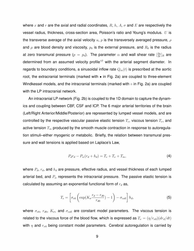
where x and r are the axial and radial coordinates, R, h, A, σ and E are respectively the
vessel radius, thickness, cross-section area, Poisson’s ratio and Young’s modulus. U is
the transverse average of the axial velocity u, p is the transversely averaged pressure, ρ
and µ are blood density and viscosity, p0 is the external pressure, and R0 is the radius
at zero transmural pressure (p = p0). The parameter α and wall shear rate [∂u∂r]R are
determined from an assumed velocity profile17 with the arterial segment diameter. In
regards to boundary conditions, a sinusoidal inflow rate Qin(t) is prescribed at the aortic
root, the extracranial terminals (marked with • in Fig. 2a) are coupled to three-element
Windkessel models, and the intracranial terminals (marked with ◦ in Fig. 2a) are coupled
with the LP intracranial network.
An intracranial LP network (Fig. 2b) is coupled to the 1D domain to capture the dynam-
ics and coupling between CBF, CSF and ICP. The 6 major arterial territories of the brain
(Left/Right Anterior/Middle/Posterior) are represented by lumped vessel models, and are
controlled by the respective vascular passive elastic tension Te, viscous tension Tν , and
active tension Tm produced by the smooth muscle contraction in response to autoregula-
tion stimuli–either myogenic or metabolic. Briefly, the relation between transmural pres-
sure and wall tensions is applied based on Laplace’s Law,
Pdrd − Pic(rd + hd) = Te + Tν + Tm, (4)
where Pd, rd, and hd are pressure, effective radius, and vessel thickness of each lumped
arterial bed, and Pic represents the intracranial pressure. The passive elastic tension is
calculated by assuming an exponential functional form of rd as,
Te =
[σe0
(exp(Kσ
rd − rd0rd0
)− 1
)− σcoll
]hd, (5)
where σe0, rd0, Kσ, and σcoll are constant model parameters. The viscous tension is
related to the viscous force of the blood flow, which is expressed as Tν = (η/rν0)(drd/dt)
with η and rν0 being constant model parameters. Cerebral autoregulation is carried by
9

smooth muscle producing an elastic tension as,
Tm = T0(1 +M) exp
(−∣∣∣∣rd − rmrt − rm
∣∣∣∣nm)
(6)
where T0, rt, rm, and nm are constant model parameters, and M is the autoregulation
activation factor responding to maintain CBF, which varies between [-1, 1] and can be
calculated by,
M =e2x − 1
e2x + 1. (7)
The extreme values of M , 1 and -1, represent maximal vasoconstriction and vasodila-
tion. To maintain CBF, the control function is modeled with a first-order low pass system
expressed as,
tCAdx
dt= −x+GCA
qd − qnqn
, (8)
where qd is the CBF at each cerebral territory, and qn is the respect target flow rate. tCA
and GCA are constant parameters representing the time scale and gain of the low pass
filter, respectively.
ICP Pic is spatially uniform within the intracranial compartment and shared by the
six distal vascular beds. The ICP and its coupling with the cerebral vascular system
are determined by the Monro-Kellie principle, assuming that the total volume inside the
cranium remains constant, which can be represented as follows,
CicPicdt
=6∑
k=1
(dVkdt
+ Ifk
)− I0 (9)
where k represents the indices of six distal vascular beds, Vk is the blood volume of
vascular bed k, Ifk and I0 are CSF inflow and outflow, respectively. The intracranial
compliance Cic is modeled as a nonlinear function of ICP. The volume changes of Vk is
represented by a differential equation of effective vessel radius rd of each vascular terri-
tory, which varies due to blood pressure and myogenic or metabolic autoregulation. This
cerebrovascular model has been validated against clinical measurements of a transient
10

hyperemic response test11, which quantifies the dynamics change of CBFV in the right
MCA due to transient compression of the carotid artery. Additionally, qualitative validation
of the model with regards to CO2 inhalation and hyperventilation tests have also been
performed35. Further implementation details and nominal parameter assignment for this
model can be found in34.
This multi-scale model is potentially advantageous for several reasons. A distributed
1D network for modeling the major systemic and cerebral arteries facilitates data assimila-
tion. Namely, measurements of blood flow or pressure from specific arteries can be more
directly assimilated to corresponding locations in the model. Moreover, the 1D distributed
network enables more realistic pressure and flow temporal waveforms37, and therefore,
measurements of (e.g., CBFV or ABP) temporal waveform dynamics can be better assim-
ilated, potentially better informing model calibration and ICP estimation. These pressure
and flow waveforms are also the main “forcing functions” to intracranial dynamics. The
multi-scale model also enables more avenues to make the model patient-specific from,
e.g., angiography, or other clinically-available data.
2.3 Regularizing iterative ensemble Kalman method
Data-assisted predictions of unobserved states and parameters can be considered pos-
terior estimations calculated from the prior (Eq. 1) and data (Eq. 2) using Bayes’ theorem
p(x|y) ∼ p(x)p(y|x), (10)
where p(x|y), p(x), and p(y|x) are the probability density functions of the posterior state,
prior state, and data uncertainty, respectively. To obtain the exact posterior estimation,
Markov chain Monte Carlo (MCMC) sampling is typically required to sample the poste-
rior distribution. This process involves an onerous number of forward model evaluations
sequentially, which is prohibitively expensive for nontrivial systems. As such, we adopt
an approximate Bayesian approach, the iterative ensemble Kalman method (IEnKM)19,
11
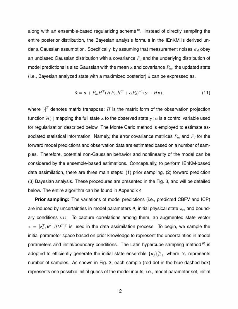
along with an ensemble-based regularizing scheme18. Instead of directly sampling the
entire posterior distribution, the Bayesian analysis formula in the IEnKM is derived un-
der a Gaussian assumption. Specifically, by assuming that measurement noises σd obey
an unbiased Gaussian distribution with a covariance Pd and the underlying distribution of
model predictions is also Gaussian with the mean x and covariance Pm, the updated state
(i.e., Bayesian analyzed state with a maximized posterior) x can be expressed as,
x = x + PmHT (HPmH
T + αPd)−1(y −Hx), (11)
where [·]T denotes matrix transpose; H is the matrix form of the observation projection
function H(·) mapping the full state x to the observed state y; α is a control variable used
for regularization described below. The Monte Carlo method is employed to estimate as-
sociated statistical information. Namely, the error covariance matrices Pm and Pd for the
forward model predictions and observation data are estimated based on a number of sam-
ples. Therefore, potential non-Gaussian behavior and nonlinearity of the model can be
considered by the ensemble-based estimations. Conceptually, to perform IEnKM-based
data assimilation, there are three main steps: (1) prior sampling, (2) forward prediction
(3) Bayesian analysis. These procedures are presented in the Fig. 3, and will be detailed
below. The entire algorithm can be found in Appendix 4
Prior sampling: The variations of model predictions (i.e., predicted CBFV and ICP)
are induced by uncertainties in model parameters θ, initial physical state zo, and bound-
ary conditions ∂D. To capture correlations among them, an augmented state vector
x = [zTo ,θT , ∂DT ]T is used in the data assimilation process. To begin, we sample the
initial parameter space based on prior knowledge to represent the uncertainties in model
parameters and initial/boundary conditions. The Latin hypercube sampling method20 is
adopted to efficiently generate the initial state ensemble {xj}Nsj=1, where Ns represents
number of samples. As shown in Fig. 3, each sample (red dot in the blue dashed box)
represents one possible initial guess of the model inputs, i.e., model parameter set, initial
12
Parameter space
Samples from prior distribution (initial guess)
:
Forward model of intracranial dynamics
Foward propagation
Updated state ensemble
Predicted state ensemble
State space
Observation space
CBFV at all arteries
ICP
model parameters
:CBFV at MCA
y =
H(x
)
y
x
State spaceTCD data
Kalm
an
form
ula
Iterations
Prior Sampling Step Forward Prediction Step Bayesian Analysis Step
1
2
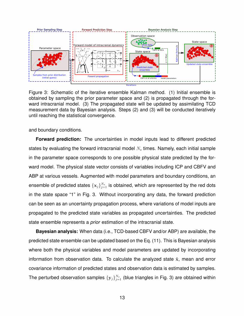
Figure 3: Schematic of the iterative ensemble Kalman method. (1) Initial ensemble isobtained by sampling the prior parameter space and (2) is propagated through the for-ward intracranial model. (3) The propagated state will be updated by assimilating TCDmeasurement data by Bayesian analysis. Steps (2) and (3) will be conducted iterativelyuntil reaching the statistical convergence.
and boundary conditions.
Forward prediction: The uncertainties in model inputs lead to different predicted
states by evaluating the forward intracranial model Ns times. Namely, each initial sample
in the parameter space corresponds to one possible physical state predicted by the for-
ward model. The physical state vector consists of variables including ICP and CBFV and
ABP at various vessels. Augmented with model parameters and boundary conditions, an
ensemble of predicted states {xj}Nsj=1 is obtained, which are represented by the red dots
in the state space “1” in Fig. 3. Without incorporating any data, the forward prediction
can be seen as an uncertainty propagation process, where variations of model inputs are
propagated to the predicted state variables as propagated uncertainties. The predicted
state ensemble represents a prior estimation of the intracranial state.
Bayesian analysis: When data (i.e., TCD-based CBFV and/or ABP) are available, the
predicted state ensemble can be updated based on the Eq. (11). This is Bayesian analysis
where both the physical variables and model parameters are updated by incorporating
information from observation data. To calculate the analyzed state x, mean and error
covariance information of predicted states and observation data is estimated by samples.
The perturbed observation samples {yj}Nsj=1 (blue triangles in Fig. 3) are obtained within
13

the observation space spanned by measurement uncertainties and process errors. Note
that only a very limited portion of the state is observed (e.g., CBFV at MCA), and thus the
dimension of observation vector y is much smaller than that of the full state vector x, as
shown in Fig. 3. Finally, the updated state ensemble is in turn used as the initial ensemble
in next iteration of the IEnKM.
Iterative regularization scheme: The forward prediction and Bayesian analysis steps
are conducted iteratively until a prescribed stopping criterion. To stabilize the Bayesian
update and control the iterative process, a regularization scheme proposed in18 was
adopted. Specifically, the control variable α in Eq. 11 is calculated by the following se-
quence,
αi+1 = 2iα0, (12)
where α0 is an initial guess. Then, we chose α = αN , where N is the first integer such
that,
αN ||P−1/2d (HPmH
T + αNPd)−1(y −Hx)||2 ≥ ρ||P−1/2
d (y −Hx)||2, (13)
where || · ||2 represents L2 norm, and ρ is a constant parameter within an interval of (0, 1).
Larger ρ indicates slowly decaying α and thus more regularization on the Bayesian anal-
ysis. The iteration is terminated whenever the normalized misfit between prediction and
data is smaller than the noise level of the data, as shown by Eq. 22. This regularization
scheme can be derived as an approximation of the regularizing Levenberg-Marquardt
scheme30, where the derivative of the forward operator and its adjoint are approximated
using ensemble-based covariances. The details of associated derivations and proofs can
be found in18.
3 Results
We first consider synthetic data to systematically explore the proposed framework. Our
goal is to test if the assimilation of middle cerebral artery (MCA) blood flow velocity, which
14

is readily accessible clinically, is sufficient to improve prediction of ICP in the model. Note,
it is not obvious that assimilation of MCA CBFV data alone (and even if the data is noise-
free) can lead to significant improvement in ICP prediction since the intracranial model is
highly nonlinear, and MCA flow velocity has no direct relation to ICP. We then proceed
to a more realistic application, using patient-specific TCD data measured clinically in pa-
tients suspected of having intracranial hypertension. These patients also had invasive
ICP measurements performed that the model prediction can be compared against.
Based on a parameter sensitivity analysis (see Table. 1) for the intracranial model by
the one-factor-at-a-time (OFAT) method, we identified that the target perfusion flow rate
parameters qn (see Eq. 8) of the six arterial territories are important for both CBFV and
ICP prediction. (Note, this does not necessarily imply CBFV is dominant in ICP predic-
tion.) To improve identifiability of the problem, only the six primary parameters qn are
inferred simultaneously along with the hidden ICP state. Other parameters, which were
deemed less important by the sensitivity analysis were determined offline from population-
based calibrations conducted in previous studies14,40. The full set of primary parameters
for both the forward intracranial model and the data assimilation process are given by
Table 2.
Table 1: Sensitivity of primary model parameters to CBFV and ICP. Specifically, each pa-rameter is uniformly perturbed by 20 percent of its baseline value, and the correspondingperturbations of CBFV and ICP are presented.
Parameters rd0 σe0 Kσ σcoll η T0 tCA GCA qn
CBFV 1.25% 0.02% 0.05% 0.60% 0.28% 3.58% 0.01% 0.16% 35.57%ICP 0.90% 0.03% 0.04% 0.52% 0.03% 2.89% 0.02% 0.05% 30.83%
3.1 Verification with synthetic data
The intracranial model was run using an arbitrary but physiologic set of model parameters
as the “ground truth”. That is, instead of data coming from a patient, data comes from the
model run with a hidden parameter set. The six unknown “true” target flow rate parame-
15

Table 2: Primary parameters of forward model and data assimilation
Baseline values of forward intracranial model
rd0 = 0.015 cm σe0 = 0.1425 cm Kσ = 10.0σcoll = 62.79 mm Hg η = 232 mm Hg T0 = 2.16 mm Hg cmrt = 0.018 cm rm = 0.027 cm tCA = 10 sGCA = 10 mm Hg−1 qn = 2.2 (MCAs), 1.48 (ACAs), 1.14 (PCAs) ml s−1
Parameters of data assimilation (IEnKM)
prior uncertaintiy 20% uniformly random perturbationnumber of samples Ns 20regularization parameters ρ = 0.6, α0 = 1
ters are shown as black lines in Fig. 4. Synthetic TCD data was obtained by “measuring”
CBFV at the left and right MCAs, with and without artificial random noises added. Then
all simulated information is discarded, except the measured MCA CBFV data, and the
ICP which was blinded and reserved as the “ground truth” to later compare against. To
determine the sample size sufficient for an accurate mean estimation, data assimilation
using Ns = 20, 50, and 100 samples was conducted and the expectations of posterior ICP
estimations are compared. The results showed that the difference among these cases
was less 2%. Therefore, twenty samples (Ns = 20) were adopted in the following numeri-
cal cases. Note that the term “sample” represents one of the randomly perturbed forward
simulations in IEnKM, while the term “data” refers to the noninvasive measurements within
this paper.
3.1.1 Noise-free CBFV data
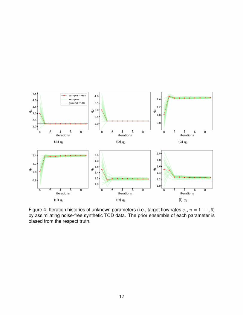
We first consider the case in which the MCA CBFV measurements are noise-free. Fig-
ure 4 shows DA iteration histories of the target flow rate parameters qn, n = 1, · · · , 6,
which are added to the extended state vector and inferred during the DA process. All
the samples (light green lines) are scattered initially (iteration step 0), representing the
prior distributions of the parameters. Each ensemble mean at iteration step 0 (first red
dot) can be seen as a best prior guess for the respective parameter; it is observed that
16
(a) q1 (b) q2 (c) q3
(d) q4 (e) q5 (f) q6
Figure 4: Iteration histories of unknown parameters (i.e., target flow rates qn, n = 1 · · · , 6)by assimilating noise-free synthetic TCD data. The prior ensemble of each parameter isbiased from the respect truth.
37
Figure 4: Iteration histories of unknown parameters (i.e., target flow rates qn, n = 1 · · · , 6)by assimilating noise-free synthetic TCD data. The prior ensemble of each parameter isbiased from the respect truth.
17

these prior guesses deviate significantly from the respective ground truths (black lines),
representing a typical biased prior estimation. The bias is highly relevant in real-world ap-
plications, since it is almost impossible to guarantee an unbiased prior (initial guess for a
de novo patient). However, after assimilating the synthetic TCD velocity “measurements”
at the MCAs, the unknown parameters are well recovered within a few iterations and un-
certainty is largely reduced. As expected, CBFV data in the MCAs is most informative to
MCA-related target flow rates (q1 and q2), which converge exactly to the truth, whereas
slight discrepancies remain for ACA and PCA territory perfusion flow rates (q3 – q6).
(a) prior (b) posterior (noise-free, MCAs) (c) posterior (noisy, MCAs)
(d) posterior (noise-free, one MCA) (e) posterior (noisy, one MCA)
Figure 5: Comparison of (a) prior ICP prediction and posterior ICP predictions following(b) noise-free, two MCAs, (c) noisy, two MCAs, (d) noise-free, right MCA and (e) noisy,right MCA CBFV data assimilations.R2
38
Figure 5: Comparison of (a) prior ICP prediction and posterior ICP predictions following(b) noise-free, two MCAs, (c) noisy, two MCAs, (d) noise-free, right MCA and (e) noisy,right MCA CBFV data assimilations.
We next consider the hidden state of most interest, ICP, which is less directly related to
CBFV than the hidden parameters qn. The comparison of prior and posterior estimations
for ICP are presented in Fig. 5. In Fig. 5a, it can be observed that the prior samples of ICP
prediction are scattered from around 8.5 mmHg to 12.0 mmHg due to physiologic pertur-
bations of the initial state and parameters due to prior epistemic uncertainty. Similarly, the
18
mean (red dashed) of the prior ICP ensemble is biased from the truth (black solid). Fig. 5b
displays the convergence of each sample following assimilation of the MCA CBFV data,
demonstrating that all the posterior samples converge to the truth after the regularizing
iterative ensemble Kalman DA method is applied with very low uncertainty and expected
value very close to the true value. We note that the other hidden physical states, including
flow velocity and pressure at unobserved arteries, were also similarly recovered via this
framework; since the prediction performance is similar to that shown here for ICP, those
results are omitted.
Assimilating data from both MCAs was considered in the synthetic tests since such
simultaneous measurements can, in theory, be obtained clinically. Alternatively, we also
consider data from only one MCA, which is more consistent with the clinical cases consid-
ered below in Section 3.2. Results from the synthetic tests with only the right MCA CBFV
data assimilated are presented in Fig. 5, with the results from noise-free data in panel (d)
and from noisy data in panel (e). As shown, the posterior mean of ICP maintains close
consistency with the true ICP. However, the posterior sample scattering is slightly higher
compared to the case with data from both MCAs assimilated (Fig. 5, panels b and c).
This demonstrates that the epistemic uncertainties resulting from the lack of data can be
reasonably considered in the current Bayesian framework.
3.1.2 Noisy CBFV data
We next consider corrupting the synthetic MCA CBFV data with 10% Gaussian random
noise to represent measurement error, and in addition a 10% process error is considered
to account for potential model-form uncertainties. The combination of the measurement
error and process error are reflected by the data error covariance matrix Pd 9. We focus
here on our ultimate target of ICP. Figure 5c displays the ICP posterior estimation following
assimilation of the noisy MCA CBFV data. It is clear that all ICP samples, which as
above demonstrate high scatter in the prior estimation, converge toward the true signal by
incorporating the (now noisy) CBFV data, and that the associated posterior uncertainties
19
are largely reduced. However, compared to the results of the noise-free case as shown in
Fig. 5b, where all posterior ICP samples converge to the truth, the posterior ICP samples
in Fig. 5c display some scatter, or posterior uncertainty. Nonetheless, all samples and the
expectation are close to the truth. Moreover, if only the data from one MCA is assimilated,
a higher posterior uncertainty (i.e., higher sample scatter) is observed in Fig. 5e, which is
expected due to the reduction of data.
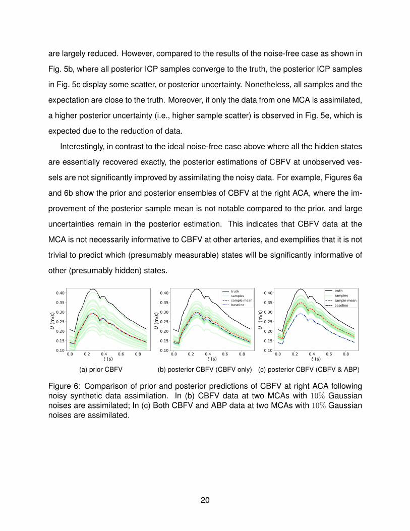
Interestingly, in contrast to the ideal noise-free case above where all the hidden states
are essentially recovered exactly, the posterior estimations of CBFV at unobserved ves-
sels are not significantly improved by assimilating the noisy data. For example, Figures 6a
and 6b show the prior and posterior ensembles of CBFV at the right ACA, where the im-
provement of the posterior sample mean is not notable compared to the prior, and large
uncertainties remain in the posterior estimation. This indicates that CBFV data at the
MCA is not necessarily informative to CBFV at other arteries, and exemplifies that it is not
trivial to predict which (presumably measurable) states will be significantly informative of
other (presumably hidden) states.
0.0 0.2 0.4 0.6 0.8t (s)
0.10
0.15
0.20
0.25
0.30
0.35
0.40
U(m
/s)
(a) prior CBFV
0.0 0.2 0.4 0.6 0.8t (s)
0.10
0.15
0.20
0.25
0.30
0.35
0.40
U(m
/s)
truth
samples
sample mean
baseline
(b) posterior CBFV (CBFV only)
0.0 0.2 0.4 0.6 0.8t (s)
0.10
0.15
0.20
0.25
0.30
0.35
0.40
U(m
/s)
truth
samples
sample mean
baseline
(c) posterior CBFV (CBFV & ABP)
Figure 6: Comparison of prior and posterior predictions of CBFV at right ACA followingnoisy synthetic data assimilation. In (b) CBFV data at two MCAs with 10% Gaussiannoises are assimilated; In (c) Both CBFV and ABP data at two MCAs with 10% Gaussiannoises are assimilated.
39
Figure 6: Comparison of prior and posterior predictions of CBFV at right ACA followingnoisy synthetic data assimilation. In (b) CBFV data at two MCAs with 10% Gaussiannoises are assimilated; In (c) Both CBFV and ABP data at two MCAs with 10% Gaussiannoises are assimilated.
20

3.1.3 Assimilating additional ABP data
The cases showed above only utilize CBFV data in the MCAs, which is commonly mea-
surable by TCD ultrasonography. Other than the TCD-based CBFV data, systemic ABP
measurements are also among the data available bedside in routine clinical practice.
Therefore, it is also interesting to investigate whether the posterior predictions can be
further improved by assimilating both ABP and CBFV measurements simultaneously. We
conducted another experiment with the same set up as above, except using both CBFV
and ABP data sampled from two MCAs. By additionally incorporating the ABP data, per-
formance of the ICP prediction remained excellent, and additionally posterior estimations
of CBFV at unobserved arteries were notably improved. For example, Figure 6c shows
the posterior ensemble of CBFV at the right ACA by assimilating both CBFV and ABP
data at the MCAs. All the samples are corrected toward the ground truth and the poste-
rior mean is significantly improved compared to the results displayed in Fig. 6b. Moreover,
sample scattering is also relatively smaller. Note that the ABP assimilated in our model
was arterial pressure at the MCA whereas systemic ABP data are typically measured at
the radial artery, which differ in time and waveform. A correction algorithm proposed by
Kashif et al.22 needs to be employed to obtain an approximation of ABP at MCAs when
systemic ABP data measured from the radial artery are used.
3.2 Validation against clinical data
Preliminary clinical application of the proposed framework was also investigated. TCD
measurements were obtained in patients that had invasive ICP measured. Note, only
right MCA CBFV was assimilated in these validation studies, compared to both left and
right MCA data being assimilated in the synthetic cases above. Generally, the prior model
parameters and overall framework were the same as in the synthetic test cases, except
the observation data to be assimilated. However, the main difference here from synthetic
cases is not just that real versus synthetic TCD data was used, but that the ICP we
21

compare against was measured from actual patients, and not the computational model.
The TCD and ICP data were acquired by the protocol approved by the UCLA Internal
Review Board and the full dataset was reported in23. In this study, we focus on patients
with a homeostatic intracranial system, where the ICP/CBFV waveform is assumed to
have reproducible features at similar mean levels13. We investigate two patients with ap-
proximate homeostatic TCD and ICP signals. The two patients are referred to as P1 and
P2. Patient P1 was a 55 years-old female and treated for aneurysmal subarachnoid hem-
orrhage (aSAH), while patient P2 was a 47 years-old male and treated for traumatic brain
injury (TBI). The ICP signals for both patients were obtained through external ventricle
drainage (EVD). Figure 7a displays the raw TCD-measured CBFV signal at right MCA
zoomed-in view
(a) raw TCD CBFV of Patient P1
(b) aggregated CBFV of patient P1 (c) aggregated CBFV of patient P2
Figure 7: TCD CBFV data. (a) Raw TCD-based CBFV signals at right MCA of the patientP1 over 260 cardiac cycles. (b-c) Aggregated CBFV pulses at the right MCA and itsensemble averaged for (b) patient P1 and (c) patient P2.
40
Figure 7: TCD CBFV data. (a) Raw TCD-based CBFV signals at right MCA of the patientP1 over 260 cardiac cycles. (b-c) Aggregated CBFV pulses at the right MCA and itsensemble averaged for (b) patient P1 and (c) patient P2.
for patient P1 over 260 cardiac cycles. The mean CBFV level approximately remains the
22
same, and waveform features are also similar cycle to cycle, as shown in the zoomed-in
view of Fig. 7a. Similar steady features are also observed in the corresponding ICP signal
and for the MCA CBFV and ICP data for patient P2.
Based on the quasi-steady nature of the signals, pulses over the 260 cardiac cycles
of raw CBFV signal data were aggregated and the ensemble average was computed.
Figures 7b and 7c show the CBFV data of patients P1 and P2 where all pulses from
the raw signal are plotted within one cardiac cycle, and the ensemble-averaged pulse is
plotted by a bold red line. The shape of the mean pulse is triphasic (i.e., having three
peaks) for both patients, which is a commonly observed feature for both CBFV and ICP
waveforms16,33,32. Although the waveforms of the MCA CBFV between the two patients
are similar, the mean CBFV level of patient P1 is slightly larger than that of patient P2.
The scattering of the pulse data represents uncertainties introduced by TCD mea-
surement errors, respiratory effects, and physiological deviations from the steady-state
assumption. These uncertainties are treated as data uncertainties in the assimilation pro-
cess and are estimated based on the pulse history. That is, instead of assimilating the
ensemble average, which would effectively ignore this uncertainty, the statistical distribu-
tion of the measured CBFV data was used to sample data for assimilation. For example,
Fig. 8a for patient P1 (and in Fig. 8c for patient P2) displays the uncertainty interval of TCD
data (light blue region) and sampled data for assimilation (green dots). As for the synthetic
cases above, the CBFV data is assimilated to calibrate target flow rate parameters, which
were deemed to be informative of ICP via the OFAT sensitivity analysis. We first compare
the ability of the model to match the measured TCD by simulating the model with the
inferred target flow rates for each patient. Without data assimilation, the prior predictions
of RMCA CBFV are highly scattered and biased, and the mean CBFVs are largely un-
derestimated for both patients, as shown in Figs. 8a and 8c. Following data assimilation,
the model parameters (i.e., target flow rates to each territory) appear well inferred as the
corresponding RMCA CBFV posterior prediction is significantly improved when compared
with the TCD data and has less uncertainty, as shown in Figs. 8b and 8d. Note that all
23

0.0 0.2 0.4 0.6 0.8t (s)
0.4
0.6
0.8
1.0
1.2
U(m
/s)
(a) Prior CBFV (P1)
0.0 0.2 0.4 0.6 0.8t (s)
0.4
0.6
0.8
1.0
1.2
U(m
/s)
samples
sample mean
baseline
TCD data
(b) Posterior CBFV (P1)
0.0 0.2 0.4 0.6 0.8t (s)
0.4
0.6
0.8
1.0
U(m
/s)
(c) Prior CBFV (P2)
0.0 0.2 0.4 0.6 0.8t (s)
0.4
0.6
0.8
1.0
U(m
/s)
samples
sample mean
baseline
observation
(d) Posterior CBFV (P2)
(e) ICP data (P1) (f) posterior ICP (P1)
(g) ICP data (P2) (h) posterior ICP (P2)
Figure 8: CBFV predictions (a-d) and ICP predictions (e-h) following assimilation of TCDCBFV measurements.
41
Figure 8: CBFV predictions (a-d) and ICP predictions (e-h) following assimilation of TCDCBFV measurements.
24
the posterior samples are mostly converged to the sample mean curve (red dashed line)
quickly. The reason for this is that the data uncertainty level is relatively large compared
to the perturbation of simulations and thus the stopping criteria can be satisfied within
only a few DA iterations. Although the posterior CBFV pulse agrees well with TCD data
and mostly falls inside the data uncertainty region, some discrepancy can be observed at
the beginning of the CBFV pulse (“early systole") in both patients. This is likely due to the
model-form error as discussed below.
Finally, we investigate the prediction of ICP for the two patients in comparison to the
invasive ICP data measured from the lateral ventricles in each patient. Similar to the TCD
data, the raw ICP pulses are aggregated to compute an ensemble average and statistical
distribution for uncertainty. Figures 8e and 8g show the ensemble-averaged pulse for the
invasive ICP measurements for patients P1 and P2, while Figs. 8f and 8h display the non-
invasive ICP predictions obtained from our data assimilation framework. For both patients,
the baseline (prior mean) ICP prediction substantially under-predicts the measured mean
ICP. However, after assimilating the TCD measurements, the posterior ICP predictions
of both patients (red curve) increase significantly, with a mean value reasonably close to
the mean invasive ICP measurements for each respective patient. Specifically, for patient
P1 (Figs. 8e and 8f), the mean ICP measurement is 12.8 mmHg and the mean of TCD-
augmented ICP prediction is 11.2 mmHg. And for patient P2 (Figs. 8g and 8h), the mean
ICP measurement is 16.2 mmHg and the mean of TCD-augmented ICP prediction is 15.9
mmHg. For both patients, the prediction error in mean ICP is within 2 mmHg, which is the
clinically-accepted ICP error standard44. Moreover, it is interesting to note that the pos-
terior ICP samples exhibit relative scatter although the corresponding CBFV samples are
mostly converged. This is because no direct ICP measurements are used in the assimi-
lation and thus relatively larger epistemic uncertainties are expected. Although mean ICP
appears well predicted and significantly improved using the framework proposed herein,
the predicted ICP waveform shape significantly differs from the measured triphasic shape.
This discrepancy is discussed below.
25

4 Discussion
We have presented a data-augmented, theory-based modeling approach for noninvasive
intracranial pressure estimation, based on a multiscale intracranial model and assimilation
of clinically-available TCD CBFV data. A regularizing iterative ensemble Kalman method
is employed for fusing the computational model with measurement data. The proposed
framework has been examined through both synthetic tests and tests with actual patient
data, both of which demonstrated that the presented assimilation procedure was able to
significantly improve mean ICP prediction.
The tests using synthetic data were conducted to verify implementations of the frame-
work and analyze the identifiability of the unknown parameters and hidden variables.
When both the forward intracranial model and measurement data are precise (i.e., no
error in the model or synthetic data), all the unknown parameters and hidden states in-
cluding unobserved CBFV and ICP can be precisely recovered by only assimilating CBFV
data at the MCAs and associated uncertainties due to prior perturbations in model pa-
rameters can be nearly eliminated. For a more realistic condition, where both the forward
model and measurement data were made imprecise through the introduction of a 10%
error, strong performance of ICP prediction was maintained. Namely, the posterior mean
of the ICP agreed well with the ground truth, however uncertainty in the posterior ICP
prediction increased due to the uncertainties introduced by the model inadequacy and
measurement noise. Nonetheless, the results demonstrate that overall the ICP prediction
can be significantly improved by incorporating noninvasive CBFV data, and uncertain-
ties associated with the data and model can be naturally considered within the Bayesian
framework presented.
Based on the results of the synthetic tests, CBFV data at MCAs were demonstrated
to be informative to ICP predictions. However, they appeared less informative to CBFV
at other unobserved arterials, e.g., ACAs, when data were corrupted by random noise.
Although ICP can be accurately predicted, the improvement of posterior predictions of
26

CBFV at unobserved arterials was not remarkable and uncertainties remained consider-
able after data assimilation. However, by additionally incorporating ABP data along with
CBFV data at MCAs, predictions of CBFV at ACAs were significantly improved. These
results indicate that assimilating more independent information can further enhance hid-
den state estimation and reduce associated epistemic uncertainties. The assimilations
of multiple noninvasive signals is something to be further explored to broaden or further
improve the utility of this framework.
Actual TCD and invasive ICP measurements from two patients with approximate home-
ostatic intracranial dynamics were used to examine the feasibility of the proposed ap-
proach toward clinical application. The performance of the proposed approach in these
patient-based cases was promising. The data assimilation procedure led to significant
improvement in mean ICP prediction, with a posterior estimate of mean ICP close to the
invasively measured mean value and within the current clinical standard for ICP error.
These results indicate that noninvasive ICP prediction can be informed by CBFV data,
and implies that the perfusion blood flow distribution among the six major vascular terri-
tories appears to be a significant factor in steady-state ICP dynamics. While the focus
of this paper is the theoretic basis and methodology of the data-augmented nICP frame-
work, these clinical comparisons, although limited, demonstrate feasibility of the proposed
approach. Nonetheless, additional validations are needed to properly establish clinical vi-
ability of this approach.
It should be noted that although mean ICP prediction matched reasonably with that
from invasive measurement, the shape of the measured ICP waveform was not well repli-
cated. This may be expected for several reasons. First, the shape of the posterior pre-
diction for the MCA CBFV waveform differed (albeit to less degree) from the measured
waveform (Figs. 8b and 8d). This is potentially due to the simplified sinusoidal waveform
used at the aortic root, which essentially drives waveform dynamics to the rest of the
model. While it is possible to impose a more physiologic waveform at the aortic root, ide-
ally these dynamics should arise naturally from the model assuming that an appropriate
27

“unadulterated" waveform can be imposed, since the measured aortic waveform already
contains reflected waves, which would be confounded by reflections generated from the
1D network model. Second, ICP modeling herein was highly simplified, which likely con-
tributes to the damped dynamics of the ICP waveform. In our model, intracranial pressure
and CSF was modeled as spatially uniform and shared by the six distal vascular beds.
CFS (and hence ICP) dynamics were governed by simple conductances at the capillary
outlets and venous return. This is a significant simplification and in reality ICP dynamics
is likely influenced by the multi-ventricular flow of CSF and dynamic coupling with brain
tissue and different arterial territories. Hence, it is expected that the forward model should
be geared toward improved ICP dynamics modeling by considering expanded modeling
of the CFS circulation and dynamic coupling with the brain and other tissues. (Indeed, the
computed and measured CBFV waveforms agreed much more closely, even without cal-
ibration, as the intracranial model employed was more hemodynamics-oriented.) This is
a significant undertaking and will be pursued in a separate work, however, it is important
to note that mean ICP is generally used clinically for diagnosis of intracranial hyperten-
sion. Nonetheless, it is expected that improved modeling of CSF and ICP dynamics will
improve the predictive capabilities of even mean ICP, and moreover emerging research8,3
is recognizing the importance of ICP waveform analysis for diagnosis and differentiation
of cerebral pathologies and treatment management.
In regards to numerical implementation, the majority of the forward intracranial model
dynamics is implemented in C++, where the 1D distributed network is solved using an
in-house finite volume solver and the LP intracranial portion is solved using an open-
source ODE solver of a C++ library SUNDIALS36. The in-house data assimilation solver,
i.e., IEnKM, was implemented in Python. The computational cost of this implementation
mainly depends on the number of samples used for Kalman updates, since each sample
involves a forward simulation. As mentioned above, Ns = 20 samples are used in this
work and approximately three to five iterations are needed to achieve statistical conver-
gence. Therefore, each data assimilation case may involve approximately 100 forward
28

model evaluations, which entails running the model until it reaches homeostatic intracra-
nial state. If starting from the steady state of the baseline case, each perturbed case
typically converges in less than five cardiac cycles. On a single CPU core, it takes about
40 seconds to simulate one cardiac cycle. However, the propagation of case ensemble
can be done in parallel. In this work, a dual-processor with 20 CPU cores was used and
thus each data assimilation case took approximately 15 minutes. However, computational
efficiency has not yet been a focus, since the objective of this work has been to explore
feasibility.
A Algorithm: regularizing iterative ensemble Kalman method
Prior sampling: Use Latin hypercube sampling method to generate the prior state en-
semble {x(0)j }Ns
j=1, where xj is jth sample of the augmented state, including major arterials’
CBFV and ABP, ICP, and unknown parameters. Let ρ ∈ (0, 1) and τ = 1/ρ.
For n = 1 : nmax
1. Forward prediction:
(a) Evaluate the forward intracranial model with the initial physical state, boundary
conditions, and model parameters, which are updated in the last iteration. Namely,
the analyzed state x(n)j at iteration step n is propagated through the forward model
F at (n+ 1)th iteration,
x(n+1)j = F(xnj ). (14)
(b) Obtain the perturbed ensemble of observation data {y(0)j }Ns
j=1 based on the data
uncertainty level σd.
(c) Calculate statistical information of predicted state and observation data. We first
29

calculate the sample means of state and data as,
x(n+1) =1
Ns
Ns∑j=1
x(n+1)j (15)
y(n+1) =1
Ns
Ns∑j=1
y(n+1)j . (16)
The error covariances of the predicted state and observation data can then be ob-
tained,
P (n+1)m =
1
Ns − 1
N∑j=1
(x(n+1)j − x)(x
(n+1)j − x(n+1))T (17)
P(n+1)d =
1
Ns − 1
N∑j=1
(y(n+1)j − y)(y
(n+1)j − y(n+1))T (18)
2. Regularizing Bayesian analysis:
(a) Calculate the control variable α(n+1)i by following sequence,
α(n+1)i = 2i+1α0, (19)
where an initial guess of α0 = 1 is used in this work. The αn+1 is obtained as
α(n+1) ≡ α(n+1)N , where N is the first integer when the inequality defined by Eq. 13 is
satisfied. (b) Compute regularized Kalman gain matrix as,
K(n+1) = P (n+1)m HT (HP (n+1)
m HT + α(n+1)P(n+1)d )−1, (20)
(c) Update each state sample as follows,
x(n+1)j = x
(n+1)j +K(n+1)(y(n+1) −Hx
(n+1)j ), (21)
3. Stopping criteria:
30

If
||P (n+1)d
−1/2(y(n+1) −Hx(n+1))|| ≤ τσd, (22)
then, stop the iteration. σd represents noise level of observation data.
Acknowledgments
JXW would like to thank J. Pyne and J. Wu for helpful discussions. The authors also thank
the anonymous reviewers for their comments and suggestions, which helped improve the
quality and clarity of the manuscript.
References
1. Andrews, P. J., G. Citerio, L. Longhi, K. Polderman, J. Sahuquillo, P. Vajkoczy, N.-I.
Care, E. M. N. S. of the European Society of Intensive Care Medicine et al. NICEM
consensus on neurological monitoring in acute neurological disease. Intensive care
medicine 34:1362–1370, 2008.
2. Arnold, A., C. Battista, D. Bia, Y. Z. German, R. L. Armentano, H. Tran, and M. S.
Olufsen. Uncertainty quantification in a patient-specific one-dimensional arterial net-
work model: EnKF-based inflow estimator. Journal of Verification, Validation and
Uncertainty Quantification 2:011002, 2017.
3. Arroyo-Palacios, J., M. Rudz, R. Fidler, W. Smith, N. Ko, S. Park, Y. Bai, and X. Hu.
Characterization of shape differences among ICP pulses predicts outcome of external
ventricular drainage weaning trial. Neurocritical care 25:424–433, 2016.
4. Asiedu, D. P., K.-J. Lee, G. Mills, and E. E. Kaufmann. A review of non-invasive
methods of monitoring intracranial pressure. Journal of Neurology Research 4:1–6,
2014.
31
5. Bertoglio, C., P. Moireau, and J.-F. Gerbeau. Sequential parameter estimation for
fluid–structure problems: Application to hemodynamics. International Journal for Nu-
merical Methods in Biomedical Engineering 28:434–455, 2012.
6. Brandi, G., M. Béchir, S. Sailer, C. Haberthür, R. Stocker, and J. F. Stover. Tran-
scranial color-coded duplex sonography allows to assess cerebral perfusion pressure
noninvasively following severe traumatic brain injury. Acta neurochirurgica 152:965–
972, 2010.
7. Cardim, D., C. Robba, M. Bohdanowicz, J. Donnelly, B. Cabella, X. Liu, M. Cabeleira,
P. Smielewski, B. Schmidt, and M. Czosnyka. Non-invasive monitoring of intracranial
pressure using transcranial Doppler ultrasonography: is it possible? Neurocritical
care 25:473–491, 2016.
8. Connolly, M., P. Vespa, N. Pouratian, N. R. Gonzalez, and X. Hu. Characterization of
the relationship between intracranial pressure and electroencephalographic monitor-
ing in burst-suppressed patients. Neurocritical care 22:212–220, 2015.
9. Dennis, B., J. M. Ponciano, S. R. Lele, M. L. Taper, and D. F. Staples. Estimating
density dependence, process noise, and observation error. Ecological Monographs
76:323–341, 2006.
10. Ghajar, J. Traumatic brain injury. The Lancet 356:923–929, 2000.
11. Giller, C. A. A bedside test for cerebral autoregulation using transcranial doppler
ultrasound. Acta neurochirurgica 108:7–14, 1991.
12. Hickman, K., B. Mayer, and M. Muwaswes. Intracranial pressure monitoring: review
of risk factors associated with infection. Heart & lung: the journal of critical care
19:84–90, 1990.
13. Hu, X., N. Gonzalez, and M. Bergsneider. Steady-state indicators of the intracra-
32

nial pressure dynamic system using geodesic distance of the icp pulse waveform.
Physiological measurement 33:2017, 2012.
14. Hu, X., V. Nenov, M. Bergsneider, T. C. Glenn, P. Vespa, and N. Martin. Estimation of
hidden state variables of the intracranial system using constrained nonlinear Kalman
filters. IEEE transactions on biomedical engineering 54:597–610, 2007.
15. Hu, X., V. Nenov, M. Bergsneider, and N. Martin. A data mining framework of nonin-
vasive intracranial pressure assessment. Biomedical Signal Processing and Control
1:64–77, 2006.
16. Hu, X., P. Xu, F. Scalzo, P. Vespa, and M. Bergsneider. Morphological clustering
and analysis of continuous intracranial pressure. IEEE Transactions on Biomedical
Engineering 56:696–705, 2009.
17. Hughes, T. J. and J. Lubliner. On the one-dimensional theory of blood flow in the
larger vessels. Mathematical Biosciences 18:161–170, 1973.
18. Iglesias, M. A. A regularizing iterative ensemble Kalman method for PDE-constrained
inverse problems. Inverse Problems 32:025002, 2016.
19. Iglesias, M. A., K. J. Law, and A. M. Stuart. Ensemble Kalman methods for inverse
problems. Inverse Problems 29:045001, 2013.
20. Iman, R. L. Latin hypercube sampling. Encyclopedia of quantitative risk analysis and
assessment , 2008.
21. Itu, L., P. Sharma, C. Suciu, F. Moldoveanu, and D. Comaniciu. Personalized blood
flow computations: A hierarchical parameter estimation framework for tuning bound-
ary conditions. International journal for numerical methods in biomedical engineering
33, 2017.
33

22. Kashif, F. M., G. C. Verghese, V. Novak, M. Czosnyka, and T. Heldt. Model-based
noninvasive estimation of intracranial pressure from cerebral blood flow velocity and
arterial pressure. Science translational medicine 4:129ra44–129ra44, 2012.
23. Kim, S., R. Hamilton, S. Pineles, M. Bergsneider, and X. Hu. Noninvasive intracra-
nial hypertension detection utilizing semisupervised learning. IEEE Transactions on
Biomedical Engineering 60:1126–1133, 2013.
24. Kim, S., F. Scalzo, M. Bergsneider, P. Vespa, N. Martin, and X. Hu. Noninvasive
intracranial pressure assessment based on a data-mining approach using a nonlinear
mapping function. IEEE Transactions on Biomedical Engineering 59:619–626, 2012.
25. Lal, R., F. Nicoud, E. Le Bars, J. Deverdun, F. Molino, V. Costalat, and B. Moham-
madi. Non invasive blood flow features estimation in cerebral arteries from uncertain
medical data. Annals of biomedical engineering 45:2574–2591, 2017.
26. Linninger, A. A., K. Tangen, C.-Y. Hsu, and D. Frim. Cerebrospinal fluid mechanics
and its coupling to cerebrovascular dynamics. Annual Review of Fluid Mechanics
48:219–257, 2016.
27. Linninger, A. A., M. Xenos, B. Sweetman, S. Ponkshe, X. Guo, and R. Penn. A
mathematical model of blood, cerebrospinal fluid and brain dynamics. Journal of
mathematical biology 59:729–759, 2009.
28. Marsden, A. L. Optimization in cardiovascular modeling. Annual Review of Fluid
Mechanics 46:519–546, 2014.
29. Moireau, P., C. Bertoglio, N. Xiao, C. A. Figueroa, C. Taylor, D. Chapelle, and J.-F.
Gerbeau. Sequential identification of boundary support parameters in a fluid-structure
vascular model using patient image data. Biomechanics and modeling in mechanobi-
ology 12:475–496, 2013.
34
30. Moré, J. J. The Levenberg-Marquardt algorithm: implementation and theory. In:
Numerical analysis, pp. 105–116, Springer1978.
31. Pant, S., C. Corsini, C. Baker, T.-Y. Hsia, G. Pennati, and I. E. Vignon-Clementel.
Data assimilation and modelling of patient-specific single-ventricle physiology with
and without valve regurgitation. Journal of biomechanics 49:2162–2173, 2016.
32. Piper, I. R., K. Chan, I. R. Whittle, and J. D. Miller. An experimental study of cere-
brovascular resistance, pressure transmission, and craniospinal compliance. Neuro-
surgery 32:805–816, 1993.
33. Piper, I. R., J. D. Miller, N. M. Dearden, J. R. Leggate, and I. Robertson. Systems
analysis of cerebrovascular pressure transmission: an observational study in head-
injured patients. Journal of neurosurgery 73:871–880, 1990.
34. Ryu, J., X. Hu, and S. C. Shadden. A coupled lumped-parameter and distributed
network model for cerebral pulse-wave hemodynamics. Journal of biomechanical
engineering 137:101009, 2015.
35. Ryu, J., N. Ko, X. Hu, and S. C. Shadden. Numerical investigation of vasospasm
detection by extracranial blood velocity ratios. Cerebrovascular Diseases 43:214–
222, 2017.
36. Serban, R. and A. C. Hindmarsh. CVODES: the sensitivity-enabled ODE solver in
SUNDIALS. In: ASME 2005 international design engineering technical conferences
and computers and information in engineering conference, pp. 257–269, American
Society of Mechanical Engineers2005.
37. Shi, Y., P. Lawford, and R. Hose. Review of zero-D and 1-D models of blood flow in
the cardiovascular system. Biomedical engineering online 10:33, 2011.
38. Stevens, S. A., W. D. Lakin, and P. L. Penar. Modeling steady-state intracranial pres-
35

sures in supine, head-down tilt and microgravity conditions. Aviation, space, and
environmental medicine 76:329–338, 2005.
39. Tiago, J., T. Guerra, and A. Sequeira. A velocity tracking approach for the data assim-
ilation problem in blood flow simulations. International Journal for Numerical Methods
in Biomedical Engineering 33:e2856–n/a, 2017.
40. Ursino, M. and M. Giannessi. A model of cerebrovascular reactivity including the
circle of Willis and cortical anastomoses. Annals of biomedical engineering 38:955–
974, 2010.
41. Ursino, M. and C. A. Lodi. Interaction among autoregulation, CO2 reactivity, and
intracranial pressure: a mathematical model. American Journal of Physiology-Heart
and Circulatory Physiology 274:H1715–H1728, 1998.
42. Wakeland, W. and B. Goldstein. A review of physiological simulation models of in-
tracranial pressure dynamics. Computers in biology and medicine 38:1024–1041,
2008.
43. Xu, P., M. Kasprowicz, M. Bergsneider, and X. Hu. Improved noninvasive intracra-
nial pressure assessment with nonlinear kernel regression. IEEE transactions on
information technology in biomedicine 14:971–978, 2010.
44. Zhang, X., J. E. Medow, B. J. Iskandar, F. Wang, M. Shokoueinejad, J. Koueik, and
J. G. Webster. Invasive and noninvasive means of measuring intracranial pressure:
a review. Physiological measurement 38:R143, 2017.
36