designing a multi-echelon multi-period supply chain under...

Online Access: www.absronline.org/journals

*Corresponding author: H. Madani School of Industrial Engineering, College of Engineering, University of Tehran, Iran.

43

International Journal of Operations and Logistics

Management Volume 4, Issue 1

Pages: 43-71

March, 2015

e-ISSN: 2309-8023

p-ISSN: 2310-4945

Designing a Multi-Echelon Multi-Period Supply Chain under Uncertainty: A Simulation-Optimization Approach

H. Madani

School of Industrial Engineering, College of Engineering, University of Tehran, Iran

Presence of many constraints and existing uncertainties in the real world is always a barrier against properly using the potentials of supply chain to attain its main purpose such as timely responding to customers’ demands and meeting their satisfactions. This study investigates the effects of different scenarios and decisions (policies) made on supply chain performance. A Simulation-optimization approach has been used for making optimal decisions under uncertainty. According to the uncertainties in the discrete stochastic simulation and also system complexity, meta-innovative genetic algorithm was used to find the preferred parameters of supply chain. Moreover, Taguchi method is used for setting up the optimal simulation-optimization algorithm parameters. Finally, results indicate the efficiency of the proposed algorithm. The proposed algorithm of this study help policy makers to minimize demand lost under different circumstances and data uncertainty.

Keywords: Supply Chain; Simulation Optimization; Uncertainty

INTRODUCTION

There are general definitions of supply chain management. These definitions are occasionally such general that include wide range of inter and extra-organizational activities. Supply chain is a dynamic entity embedding the information flows, product and money. Word “Supply Chain” indicates a flow of materials, products, information and money from customers to retailers followed by towards distributors and wholesalers and then

towards manufacturers and suppliers and vice versa (Chaparral & Mindel, 2007).

A supply chain is a complicated network comprising from several organizations with different goals for producing and distributing the products based on customers’ demand (Simchi- Loui et al., 2003). Components of each supply chain generally include customers, retailers, distributors, manufacturers and suppliers and they

http://www.absronline.org/journals

Designing a multi-echelon multi-period supply chain under uncertainty H. Madani

44

are different based on the type of supply chain (Chaperal & Mindle, 2007).

In a supply chain, the people engaged in production and suppliers of demands mostly think about how to demand the customers’ needs, from raw materials required to production, assembly, packaging, distribution and finally sales. As a supply chain is extended, it is impossible to have an accurate prediction of exogenous dynamics and intra-chain events (Min & Zhou, 2002). This indicates the necessity of making decisions under uncertainty conditions for providing proper policies in order for meeting the needs under different limitations(Noorul Haq & Kannan, 2006). Some of such uncertainties in supply chain include uncertainty in the supply, transportation, production (downtime and interruption of production resources) and demand. Some of limitations can be usually observed in the supply chains including storage, supply and production capacity, balance and demand constraints.

Since there are many studies conducted to maximize the benefits of distributors, manufacturers and suppliers. In order for finding the best strategies in the complicated networks, it is necessary to have incentive communication and coordination among partners in the chain to attain an optimal flow of information and materials in the chain (Sari, 2008).

There are different issues in multi-echelon supply chain that different objectives could be followed according to the type and need of chain. More, there are investigated some studies conducted by different objectives in multi-echelon supply chain.

Sherbrook (1968) conducted one of the first and most important works in multi-echelon supply chain. He developed a mathematical model for determining the inventory echelons in a multi-echelon supply chain aiming to minimize the expected backorders.

Cagler et al. (2003) investigated a multi-echelon and multi-item supply chain related to a limitation of an average response time in each point of demand. Wang et al. (2007) also investigated a dual-echelon chain similar to a chain provided by Cagler et al. (2003) with average response time limitation in any demand point.

Chen and Lee (2004) provided multi-objective optimization model in multi-echelon supply chain considering the uncertainty of price and demand of the product. In a paper, You and Grossmann (2010) provided an optimal design of a multi-echelon supply chain using a mixed- integer programming model in chemical industries and related companies to the existing systems in the presence of uncertainty of customer’s demand. Providing a multi-objective model, Bejareski et al. (2009) made decision for site and capacity of factories and how goods flow I the multi-echelon and multi-period supply chain. In their paper, Tsi and jang (2013) provided a simulation-optimization model to solve a dual-echelon inventory system aiming to minimize total inventory costs. Hi and Jao (2012) decided to optimally coordinate the multi-echelon supply chain under uncertainty of demand and supply.

To solve the problems about uncertainty, researchers provided many methods as indicated in Table (1).

TABLE 1 HERE

In many previous studies such as (Petrovic, 2001; Jung et al., 2004; Van Der Zee & Van Der Vorst, 2005; Sahay & Ierapetritou, 2013; Meisel & Bierwirth, 2014), simulation and optimization techniques have been used in supply chains with uncertainties. In this study, there has been considered a tri-echelon supply chain including supply, production and sales echelons of uncertainty in each three echelons. Using discrete simulation techniques, the final objective is finding the best policies in the presence of different scenarios. Main objective is to minimize the total weight of lost demands of customers under limitations of supply, production and storage capacity and budget using hybrid algorithm, Imperialist Competitive Algorithm (ICA) and Genetic Algorithm (GA). In order for considering the monetary temporal value, there has been used of engineering economic techniques in financial and cost calculations.

Motivation and significance

Reviewing the literature, one can find out the researching gap and innovations of this study detailed as below:

Int. j. oper. logist. manag. p-ISSN: 2310-4945; e-ISSN: 2309-8023 Volume: 4, Issue: 1, Pages: 43-71

45

- Optimizing a multi-period, multi-echelon and multi-product supply chain

- Modeling a wide range of constraints including supply, production and storage capacity and budget constraints;

- Simulation optimization under uncertainty in three echelons, supply, production and sales;

- Benefiting from engineering economy techniques and involving the temporal- monetary value for increasing the accuracy of financial and expenditure calculations in budget limitation;

he statement of problem has brought in the section two. Section three of this study introduces simulation-optimization system and the obtained results are presented in section four and finally section five presented conclusion.

Problem Statement

Main objective of this study is finding optimal parameters of a tri-echelon supply chain- including supply, production and sales echelons- to minimize the lost demand of customers under uncertainty in the supply capacity of suppliers, accessing time for production (taking machine failures into account) and customers’ demand. By such explanations, the simulation system of this study comprises from three main sub-systems including supply, production and sales. Along with, it is necessary to model the theories, constraints and variables of existing decisions in each sub-system in addition to investigating and simulating the internal mechanisms of any sub-system ad their interactions. In order for accurately simulating what happens in real world, there have been considered some uncertainties which have been mentioned previously.

Following assumption have been considered during simulation and optimization of the supply chain:

- Multi-period supply chain planning and optimization;

- Possibility of storing the raw materials;

- Possibility of storing the final products;

- Supply capacities and customers’ demands seemed to be stochastic;

- Failures in the production stage and planning for repair and maintenance activities;

- Available budget in any period has been considered limited. It must be mentioned that engineering economy techniques are used for involving the temporal value of money and increasing the accuracy of financial and expenditure calculations.

Constraints of supply chain optimization process are as follows:

- Supply capacity of raw materials by suppliers;

- Storage capacity in the production centers;

- Time limits of accessing to machineries as production inputs;

- Limitation of flow balance in production centers.

SIMULATION- OPTIMIZATION APPROACH

This study aims to find the best policies in the presence of various scenarios and mentioned uncertainties in order for minimizing the total weight of lost demands of various customers. Parameters which are determining the dimensions and properties of system are listed below:


46

Indices:

r Raw

materials P

Final

products s suppliers m manufacturers c customers t

Time

periods

Parameters:

raw material

micap Storage capacity of raw materials in the manufacturing centers

final product

micap Storage capacity of end products in manufacturing centers

raw material

r Usage rate of storage capacity by raw materials

final product

p Usage rate of storage capacity by final products

rpa

Raw materials required for producing end products

pmb Usage rate of manufacturing capacity for producing final products

pcw Weight of lost demand for products and various customers

cost stom

smv Cost of conducting the raw materials from suppliers to production sites

cost mtoc

mcv

Cost of conducting end products from manufacturing sites to end user (sales)

cost

pmman Cost of manufacturing the end products in the factory

cos t

rsp Cost of purchasing raw materials

cos t

rmrh Cost of storage of raw materials in the store room in any period

cost

pmph Cost of storage of end products in the warehouse in any period

tg Available budget for any period

Ir Money devaluation coefficient in any period manufaturer

mtcap Production capacity of end product in any factory

sup 2( ,( ) )plier cap cap

rst rs rscap Normal miu Supply capacity of raw materials from suppliers

cap

rsmiu indicates the mean supply capacity of supplier s and cap

rs indicate the standard

deviation

2( , ( ) )d d

pct pc pcd Normal miu Customers’ demand for end products in any

period d

pcmiu indicates mean customer’s demand c and d

pc indicates the standard deviation

exp ( )tbf

m mtbf onential miu

Intervals of downtime in production line

interval of downtime in the factory, m, has an exponential distribution with mean oftbf

mmiu

2( ,( ) )rt rt

m m mrt Normal miu

Customers’ demand for end products in any period

rt

mmiu indicates the mean period for repairing the production line, m, and rt

m indicates its

standard deviation


47

Simulation system

Inputs

stm

rsmtx

rate of raw material conducted from any supplier

in any period to different manufacturers

pmty Rate of producing final products in factories

pmctu

The amount of products sold to customers by

manufacturers in any given time period

raw material

rmtinv

the amount of raw materials stored

in production sites in each period

final product

pmtinv

the amount of final products stored

in production sites in each period

Output

Weighted sum of lost demands is considered as the main output of the simulation system.

In order for evaluating the performance of different policies in the presence of different scenarios, the influence of values of decision variables on performance benchmarks and logical relations between components of supply chain has been simulated in MATLAB software.

Simulation Algorithm

Following algorithm is used for simulating the supply chain under uncertainty and mentioned constraints:

1. Ask the user for simulation inputs 2. Simulating the supply capacity of raw

materials in successive period using related probability distribution

3. Simulating the customers’ demand in successive periods using related probability distribution

4. Observing supply capacity of raw materials constraint

5. Update the value of raw materials conducted from suppliers to manufacturers by following equations:

supsup min(1, )

plier

rstrst stm

rsmt

m

cap

x

, ,r s t

sup( )stm stm

rsmt rsmt rstx floor x , ,r s t

6. Observing the balance in the flow of materials in production centers

- Based on rate of producing any product from any manufacturing center and usage of raw materials in end products, calculate the rate required for each raw material.

- Should the rate required of a raw materials is higher than total raw material conducted and exist in the raw materials store room in related factory, calculate the correlation factor by using following formula:

( 1)

min(1, )( )

raw material stm

rm t rsmt

srmt

pmt rp

p

inv x

y a

, ,r m t

- Reduce the manufactured rate by above mentioned correlation factor to balance the materials flow in the production nodes:

( )man

pmt pmt pmty floor y

, , | 0rpm t r a

7. Simulation of Repair and Maintenance Process in Production Lines

- Simulate the values of stochastic variables of times between failures and time of repair for each production line and obtain the actual value of production capacities by reducing the repairing time from total production capacity, and represent it by

symbol manufaturer

mtcap .

8. Applying the Production Capacity constraint


48

- Calculate the production capacity required for each production line based on values produced for final products in related production line.

- Obtain related modification coefficient by using following formula:

min(1, )( )

manufaturerman mtmt

pmt pm

p

cap

y b

,m t

- Calculate the modified values of production size in any factory using following formula:

( )man

pmt pmt mty floor y

9. Calculate and update the raw materials inventory in the warehouse of factories:

- According to the production rate of each final product and combination of products, calculate the rate required of each raw material in any factory and any period (

( )pmt rp

p

y a ).

- By following formula, obtain the raw materials inventory rate in any period:

1 1 1( )raw material stm

rm rsm pm rp

s p

inv x y a

( 1) ( )raw material raw material stm

rmt rm t rsmt pmt rp

s p

inv inv x y a

, , 1r m t

- Among the values of above mentioned inventory, upon seeing negative values, be reducing the production rate of final products consuming related raw materials, zero the inventory level of related material, then update the values consumed and raw materials inventory in any period.

- Calculate total storage capacity required for storing the raw materials in any period and any factory

( ( )raw material raw material

rmt r

r

inv ).

- According to storage capacity required

and available ( raw material

micap ), calculate the

correction coefficient and reduce the values of raw materials purchased such that rate of capacity required for storing raw materials in each production site don’t exceed from its limit.

10. Calculate the inventory of end products in the warehouse of factory and update it:

- Calculate the rate of end products conducted from any factory to whole

customers in any period ( mtc

pmct

c

x ).

- By using following formula, obtain the area of inventory of raw materials in the warehouse in any period:

1 1 1

final product mtc

pm pm pmc

c

inv y x

( 1)

final product final product mtc

pmt pm t pmt pmct

c

inv inv y x

, , 1p m t

- Among values of above mentioned inventory, when seeing a negative value, by reducing the rate of final products conducted for sales, zero the inventory level of that product.

- Calculate the total storage capacity required for storing the final products in any period and any factory

( ( )final product final product

pmt p

p

inv ).

- According to storage capacity required and

available ( raw material

micap ), calculate the

correction coefficient and reduce the values of raw materials purchased such that rate of capacity required for storing raw materials in each production site don’t exceed from its limit.

Optimization Algorithm

Evolutionary algorithms are considered as the most applicable optimization methods. In comparison, methods and software for resolving the operation research models have


49

very high sensitivities to non-linear expressions in objective function and limitation of the problem. According to many complicated relations and non-linear expressions in the simulation model of this study, however, it is clear that software for resolving the operation research models have no efficiency in optimization of this model. Consequently, based on their very low sensitivity to complexity and non-linearity of relations, evolutionary methods were selected in this system to find optimal policies.

In this study, due to the complicated nature of the problem and related objective function, there have been selected the genetic optimization algorithm. In addition, because we encounter with a discrete solution space in this study comprising the rate of purchase of raw materials, production and sales rate of final products and storage rate of raw materials and final products, exploiting from genetic algorithm (GA) instruments like crossover and mutation operators in the structure of algorithm, it is necessary to optimize the particles for intelligent search in the space of discrete solution for the problem.

Chromosomes Structure

In order for minimizing the lost demands of customers under uncertainty in the supply capacity of suppliers, available time for production- considering the possibility of failures, and customers’ demands. Presence of complicated non-linear expression in the objective function of optimization problem, random nature of the problem and necessity of stochastic simulation of system for fitting its solution to decisions (policies) and different scenarios requires using suitable meta-innovative methods to deal with such complications. Based on high efficiency of genetic algorithm in solving such problems with complicated objective functions, as indicated in the literature of this study, this meta-innovative algorithm has been chosen to

resolve the problem as introduced in this study. On the other hand, it must be noted that due to the presence of various discrete variables, it is necessary to use suitable instruments for intelligent search in the space of discrete solution. Along with, this study has used of crossover and mutation instrument of genetic algorithm.

TABLE 2 HERE

For example consider a supply Chain with the following characteristics: r=14 p=5 s=4 m=3 c=20 t=6

Total number of elements for each chromosome is reported in Table (3).

TABLE 3 HERE

It must be mentioned that sales and purchase chromosomes among five above mentioned chromosomes are considered as main chromosomes and remaining will be initialized during the simulation process according to the values given by main chromosomes to justify the reasonableness of final solution.

Randomly Generated Chromosomes

- Initializing the purchase chromosome:

Use a random figure with following discrete uniform distribution to make initial values of purchase chromosome:

[ 3 , 3 ]stm cap cap cap cap

rsmt rs rs rs rs

m

x discrete unifrom miu miu

To divide above mentioned values, make random numbers among producers as below:

0| 1

(0,1)rsmt rsmt

munifrom

Please note that parameter ( 0)rsmtP

is taken

from user as one of the algorithm parameters.

Finally, final values of purchase chromosome are given by following formula:

( )stm stm

rsmt rsmt rsmt

m

x x , ,r s t


50

- Initializing to production chromosome:

Use following formula for initializing to production chromosome:

[ 3 , 3 ] ( )d d d d

pmt pc pc pc pc

cy discrete unifrom miu miu

m

, ,p m t

Calculation of Objective Function

Use following algorithm for calculating the objective function:

1- Based on the cost of purchasing the raw materials from any supplier and size of purchase in any period, obtain total purchase of raw materials in any period.

2- Using the size of raw materials conducted from the supply sites to production and sizes of end products conducted from production to sales sites and by multiplying them in related transportation costs, calculate total cost of transportation for any period.

3- Use the multiplication of size of products produced in any factors and production costs for that factory to calculate total production cost for any period.

4- Multiply the inventory echelon of raw materials and end products in any period by corresponding cost of storing the inventory and thus obtain total cost of maintaining the inventory.

5- Use the summation of above mentioned costs to calculate total costs in any period.

6- According to the available budget in any period and considering the time value of money, obtain the deviation from budget limitation.

7- Using sold size of any product to any customer in any period and customers’ demand; calculate the size of lost demand.

8- Use the weight sum of above values to evaluate the performance of decision variables and initial policies.

Crossover Operator

When 1 and 2 are the coefficients of crossover

operator obtained from user, we have:

1 2

1

1( , ( ) )

7rt normal ,r t

2 2

2

1( , ( ) )

7t normal t

Finally, using following equation, we can make the values of purchase and production offspring chromosomes:

1 1 1 2( ) (1 )stm child stm parent stm parent

rsmt rt rsmt rt rsmtx x x , , ,r s m t

2 2( ) (1 )child child child

pmt t pmt t pmty y y , ,p m t

Mutation Operator

- Mutate purchase chromosome by using following algorithm:

1- Make a Stochastic Purchase Chromosome.

2- Mutate the mutated purchase chromosome using parameters obtained from user with stochastic purchase chromosome like crossover operator algorithm.

- Mutate Production Chromosome using following algorithm:

3- Make a stochastic production chromosome.

4- Mutate the mutated production chromosome using parameters obtained from user

( 1 ) with stochastic production chromosome like

crossover operator algorithm.

Stop Condition

Above mentioned meta-innovative algorithm continues to such extent that convergency of chromosomes during two successive decades is lower than limit defined by user or running time is higher than limit defined by user. Convergence provision in descriptive algorithm is given by:

1 1

1 2

1 1

min min

min

t t t t

t t

mean mean

mean

In above equation, tmean and mint indicate mean

and minimum value for objective function in repeat t, respectively. Coefficients α1 and α2 and convergence limit, also determine by user.


51

Meta-Innovative Combined Algorithm

Here, the code-like algorithm designed for solving above mentioned optimization solution is given:

TABLE 3B HERE

Preparing the Parameters in Genetic Algorithm

Access of an algorithm to acceptable and suitable solutions follows from different factors. Some of such factors include logic used in algorithm development and values allocated to the algorithm parameters. Quality of solutions obtained depends on the effectiveness of existing parameters in running the algorithm. Methods of designing the tests are widely used in most systems. The less is the data required in a test plan, the less is the cost and time spent for running it. Data required in a test plan is a function of number of situations of test as well as number of data required in any situation. Another measure that must be always considered when designing the tests is the rate of data collected from running the tests. This needs more data. As mentioned above, it can be concluded that a suitable test plan is a plan that provides data required for analysis and accessing to optimal conditions with minimum number of tests. Taguchi introduced main applied plans in the field of designing the tests.

Taguchi Method for Designing the Tests

Taguchi defines a test for making changes in a process for studying its effects. He thinks the most effective method for conducting the tests is multi-factor method in any time.

Different stages of conducting the test detailed as below:

• Preparing the problem and objective of doting the test;

• Planning the test;

• Designing the tests;

• Conducting the tests and data collection;

• Data analysis and determining the optimal point (optimal combination of factors)

• Running the feedback for controlling and adapting the predictions practically.

Taguchi recommends analysis of mean response for any run in external arrays as well as recommending the analysis of changes using signal to noise ratio (S/N) that properly selected and in considered as a solution variable for implementing this method. These S/N ratios originated from second order function of damage and three most applicable and standard ones include:

Best nominal: 2

210log

T

S y

N s

Bigger, better:

21

1 110log

n

iL i

S

N n y

Smaller, better: 2

1

110log

n

i

iS

Sy

N n

T

S

N is used when reduced changeability is based

on the specific value of target. L

S

N is used when

system can be optimized when solution is large as

possible and finally, S

S

N is used when system is

optimized when solution is small as possible.

Generally, Taguchi test is designed by following steps:

• Determine quality factors reviewed.

• Determine number of echelons of any factor.

• Select proper offer.

• Allocate factors and their interactions to any offer column.

• Run tests based on arrays.

• Turn the test results to….ratio and find optimal echelon of any factor.

• Run the test based on optimal factors.

Setting up the Parameters using Taguchi Method

For designing the tests, Taguchi introduced main applied designs. Taguchi’s orthogonal array


52

design standards with relatively low data and relative accuracy in estimating the optimal point and estimating the effects of factors have practically maximum application. Such advantages attracted the attention of many researchers for preparing their recommended parameters required. In this study, using Taguchi’ efficient method we could find the best parameters and operators to run the algorithms.

For this reason, it is necessary to find the parameters having main effect on algorithm’s behavior. Main parameters in the algorithm provided include: population size parameter, crossover%, mutation%, keep% and stochastic production% (stochastic production percentage depends on the crossover, mutation and keep percentages), break points 1&2, mutation points 1&2, chance of selecting elite chromosome as a parent and chance of selecting the elite chromosome for mutation. There has been considered three echelons for any parameter effective in this problem. Table 4 indicated related echelons and it is necessary to select optimal combination of these echelons for recommended algorithm.

TABLE 5 HERE

Because total possible states for determining the echelons of related parameters are 310, this may not be practically time and cost saving. Using Taguchi method therefore, total number of states required for this test, there has been considered 27 states and decision will be made by such states. Table 5 indicates 27 states proposed by Taguchi method that produced by MINITAB software. There have been defined 5 times for running any test in each echelon.

TABLE 6 HERE

And lastly, there has been drawn a Figure based on S/N ratio and any echelon by MINITAB software for each controllable factors in the designed algorithm and optimal combination of selected echelons will have 1,3,1,1,3,1,3,3,2,2, order.

FIGURE 1 HERE

Numerical results and sensitivity analysis

In previous parts, the problem has been explained. We are seeking for optimal decisions in a multi-

echelon supply chain to determine a designed network including levels of raw materials supply, products production, selling products to end customers, minimum weight of lost demands for various customers(Melo, Nickel, & Saldanha-Da-Gama, 2009). Uncertainty conditions in mentioned supply chain include uncertainty in supply, manufacturing (downtime and stop condition) and demand. Limitation of supply capacity, storage, available time of machineries as production input, balance of materials flow and available budget determines the space of solution for this problem.

In order for evaluating the simulation model and meta-innovation algorithm used, it is necessary to produce the example problems with various sizes, small to big by an intelligent and stochastic method and resolve with simulation algorithms and simulation-optimization algorithm. For this reason, there was designed an algorithm and developed in MATLAB software. Table 6 indicates the ranges of parameters in mentioned algorithm for their random production. It must be mentioned that algorithms, software and codes used in this study has been run on a system with specifications detailed as below:

Intel® Core(TM)2 Dou CPU T9300 @ 2.5 GHz 2.5 GHz and RAM 3.00 GB

TABLE 7 HERE

In above equations, continuous uniform ([a b],{m,n}) indicates a matrix with equal number of rows, number of index states, m, and number of columns equal with number of index states, n, and elements of those stochastic numbers with continuous uniform distribution and values in the intervals of [a b]. For example, , weight of lost demand of product, p for customer, c, is defined as a rounded value multiplication of following stochastic numbers:

- A linear matrix with equal number of lines and number of products that are the elements of those stochastic numbers with continuous uniform distribution in the interval of [0 1].

- A column matrix with number of lines equal with number of customers that elements of those stochastic numbers with continuous uniform distribution in the interval of [0 1].


53

- A 2D matrix with number of lines and columns equal with number of products and costumers that elements of those stochastic numbers with continuous uniform distribution in the interval of [0 1].

Separating the values of above mentioned parameter to multiplication of both stochastic number causes to simulate the influence of properties of each product (such as necessity of usage)(Towill, 1996) and each customer (importance to meeting the demands of any customer) on the weight of lost demand of a unit of product for related customer by an intelligent but stochastic. This has also been used for producing the values of other parameters(Tsay, Nahmias, & Agrawal, 1999).

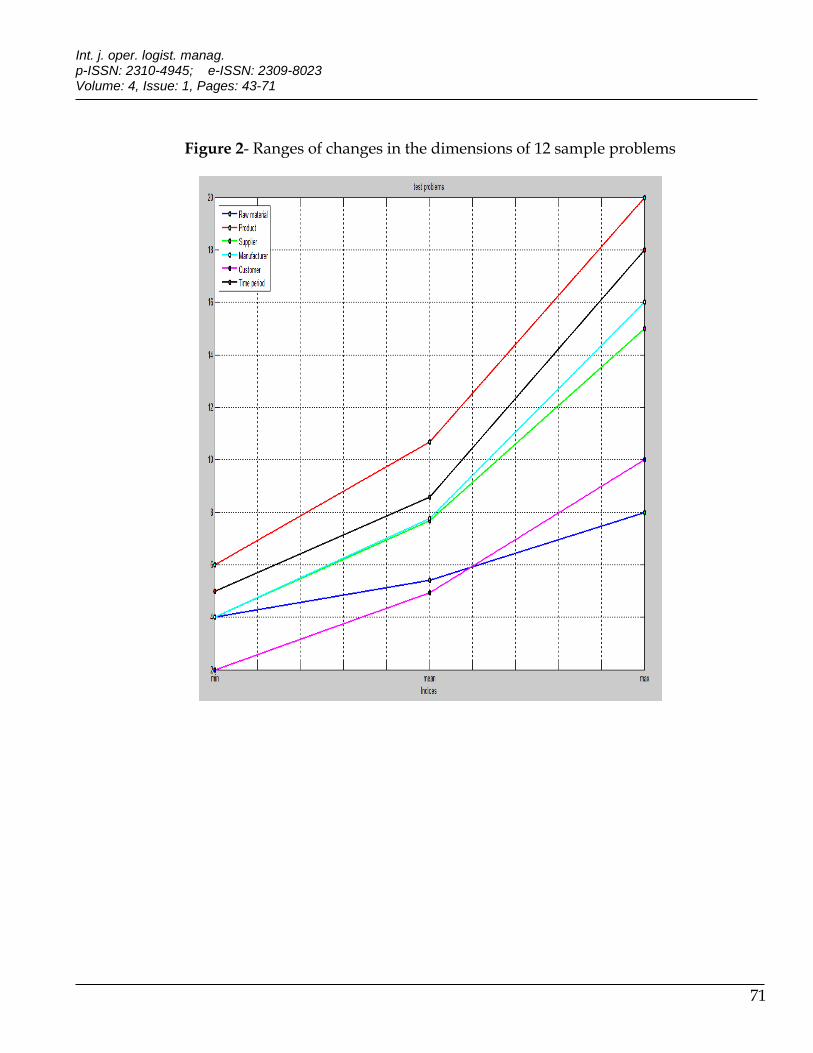
Now, to investigate the performance of simulation algorithm designed in this study, there have been made 12 sample problems with different dimensions by above mentioned algorithm. Table 7 indicates the dimensions of these sample problems.

TABLE 8 HERE

FIGURE 2 HERE

In order for evaluating the performance of simulation algorithm and code prepared in MATLAB software, above mentioned problems were prepared by different dimensions such that they include a wide range of sample problems with different complexities for solution and simulation. For example, by comparing P01 and P12, we can see that the dimensions of sample problem 12 have increased about 2 to 5 times than sample problem 1.

Table 8 indicates the summary of results for simulation of above mentioned supply chain systems. The output of simulation has been reported in the framework of costs, budget shortage rate, total weight of lost demand and running time.

TABLE 9 HERE

FIGURE 3&4 HERE

As expected, by increased dimensions of problems, total cost of chain, total weigh of lost demand and running time has been also increased. Table 8 indicates the correlation between cost of

purchasing raw materials and keeping the inventory. The main reason for such correlation in the values obtained for both cost components can be sought from close relation between concepts of such components. On the other hand, increased purchase of raw materials requires keeping the materials and additional products in the warehouses, therefore, it results in increased cost of storage. There can be also see correlations of this type between other cost components. The main reason for such correlations is the homogeneity of components drawn in Figure 4. On the other hand, increase in the dimensions of the problem results in increase in the costs of supply chain(Snyder & Shen, 2006). It must be mentioned that the time value of money has been considered in the calculations of four components of costs and budget fine.

As mentioned before, in the supply chain studied here, the values of supply capacity, available machineries’ time (downtime) and demand come with uncertainty. For this reason, by defining different echelons for mean supply capacity, downtime intervals and demand, there have been defined some scenarios detailed below to analyze the sensitivity of simulation- optimization algorithm. After defining above scenarios using simulation and optimization code prepared in MATLAB software, the optimal outputs of algorithm were determined before each scenario. Table 10 indicates such values.

TABLE 10 & 11 HERE

It can be indicated that maximum value of total weight of lost demands, despites making optimal decisions, occurs by scenarios 2, 4, 6, and 8. The common aspect in such scenarios is higher rate of customers’ demand. High rate of demand in these scenarios, indeed, as expected, caused supply chain, despites using its maximum capacities, couldn’t meet all demands and resulted in large part of demands not met. Among such scenarios, second scenario, with low supply capacity and high downtime rate lost maximum demands. On the other hand, demand lost in scenario 8, with higher demand capacity and lower downtime rate, had lower lost than other high demanding scenarios.


54

By a little attention, there can be seen the close relation between supply capacity and budget fine and cost components, particularly cost of purchasing raw materials. It is clear that for first four scenarios, with lower supply capacity, supply chain had lowest costs for purchasing the raw materials and not encountered with budget shortage at all. It must be noted that lower costs and budget fines weren’t always a promise for a proper supply chain and in some cases it indicates the inability of supply chain to meet the demands. For example, in scenarios 2 and 4, due to higher rate of demand and lower supply capacity, there was obtained maximum lost demands among 8 above mentioned scenarios; while in such optimal solution for both scenarios, there were no budget shortage in any period.

It can be generally seen an increased in the supply capacity for costs of purchasing raw materials, production and inventory control. This indicates the considerable effect of limitation in supply capacity when using potentials of mentioned chain. Comparing to other costs, by changing in the scenarios, transportation cost indicated a high fluctuation and almost a sinus form. Interestingly, there can be seen a phase difference by the size of almost one scenario between Figure of transportation cost and total weight of lost demands. On the other hand, in the scenarios with high cost of transportation incurred on supply chain, the lost demand was relatively low. This is because of a need to transporting the raw materials and final products along the chain to providing the end user with end product and preventing the lost demand.

Comparing the results obtained from simulation- optimization for scenarios 1, 2, 3, 4, 5, 6, 7 and 8 in pairwise indicates the influence of downtime rate development on lost demand. In scenarios with the same conditions, on the other hand, when the downtime rate increases, the total weight of lost demands will be increased as well.

DISCUSSION AND CONCLUSION

This study designs optimal parameters of a multi-echelon, multi-period supply chain before various limitations and uncertainty conditions. In order for dealing with uncertainty and probabilities in the

system, there was used discrete stochastic simulation instrument. To find optimal policies and decisions under different circumstances, there was used of simulation-optimization approach. In this study, we considered a tri-echelon supply chain including supply, production and sales echelons of uncertainty in each three echelons. We used discrete simulation techniques, the final objective is finding the best policies in the presence of different scenarios and such uncertainties are for minimizing the total weight of lost demands of customers under limitations of supply, production and storage capacity and budget. Meta-Innovative Genetic Algorithm was used for optimization.

Finally, it was determined that the most important factor for not meeting the demands was higher rate of its input or on the other hand, lower potentials of supply chain such as supply capacity, production and storage comparing to needed demands of customers. In this case, occurrence of many downtimes increased the gap between nominal and actual capacity of production and this made the conditions harder for meeting the demands. Instrument prepared in this study however let us use best the potentials of chain under hard circumstances to decrease the rate of lost demands. Resolving different sample problems numerically and collecting, classifying and analyzing their results reflects this fact that making optimal policies under different scenarios may have better results than making non-optimal policies under common conditions.

In order for developing this study, following theories and instruments may be used in further studies:

- Considering the distribution echelon in supply chain and related theories.

- Possibility of making strategic decisions in the supply chain such as launching production and distribution centers.

- Extending the ranges of model such that it could include the transportation Mode in the supply chain.

- Considering the uncertainties such as time required for launching the production and distribution centers and possibility of downtime of vehicles.


55

- Using other meta-innovative algorithms for making optimal decisions under different scenarios.

REFERENCES

Bertsimas, D., & Thiele, A. (2006). A robust optimization approach to inventory theory. Operations Research, 54(1), 150-168.

Bojarski, A. D., Laínez, J. M., Espuña, A., & Puigjaner, L. (2009). Incorporating environmental impacts and regulations in a holistic supply chains modeling: An LCA approach. Computers & Chemical Engineering, 33(10), 1747-1759.

Caglar, D., Li, C. L., & Simchi-Levi, D. (2004). Two-echelon spare parts inventory system subject to a service constraint. IIE Transactions, 36(7), 655-666.

Chang, M. S., Tseng, Y. L., & Chen, J. W. (2007). A scenario planning approach for the flood emergency logistics preparation problem under uncertainty. Transportation Research Part E: Logistics and Transportation Review, 43(6), 737-754.

Chen, C. L., & Lee, W. C. (2004). Multi-objective optimization of multi-echelon supply chain networks with uncertain product demands and prices. Computers & Chemical Engineering, 28(6), 1131-1144.

Chopra, S., Meindel, P. (2007). Supply chain management: Strategy, planning and operation, Pearson Prentice Hall.

Coello, C. A. C. (2005). An introduction to evolutionary algorithms and their applications. In Advanced Distributed Systems (pp. 425-442). Springer Berlin Heidelberg.

Deb, K. (2001). Multi-objective optimization. Multi-objective optimization using evolutionary algorithms, 13-46.

He, Y., & Zhao, X. (2012). Coordination in multi-echelon supply chain under supply and demand uncertainty. International Journal of Production Economics, 139(1), 106-115.

Jung, J. Y., Blau, G., Pekny, J. F., Reklaitis, G. V., Eversdyk, D. (2004). A simulation based optimization approach to supply chain management under demand uncertainty, Computer and Chemical Engineering, 28(10), 2087-2106.

Leung, S. C., Tsang, S. O., Ng, W. L., & Wu, Y. (2007). A robust optimization model for multi-site production planning problem in an uncertain environment. European Journal of Operational Research, 181(1), 224-238.

Meisel, F., Bierwirth, C. (2014). The design of Make-to-Order supply networks under uncertainties using simulation and optimization. International Journal of Production Research, (ahead-of-print), 1-18.

Mulvey, J. M., Vanderbei, R. J., & Zenios, S. A. (1995). Robust optimization of large-scale systems. Operations research, 43(2), 264-281.

Petrovic, D. (2001). Simulation of supply chain behavior and performance in an uncertain environment, International Journal of Production Economics, 71(7), 429-438.

Petrovic, D., Roy, R., & Petrovic, R. (1999). Supply chain modelling using fuzzy sets. International journal of production economics, 59(1), 443-453.

Popescu, I. (2007). Robust mean-covariance solutions for stochastic optimization. Operations Research, 55(1), 98-112.

Sahay, N., Ierapetritou, M. (2013). Supply chain management using an optimization deriven simulation


56

approach, AIChE Journal, 59(12), 4612-4626.

Santoso, T., Ahmed, S., Goetschalckx, M., & Shapiro, A. (2005). A stochastic programming approach for supply chain network design under uncertainty. European Journal of Operational Research, 167(1), 96-115.

Sari, K. (2008). On the benefits of CPFR and VMI: A comparative simulation study. International Journal of Production Economics, 113(2), 575-586.

Schultmann, F., Fröhling, M., & Rentz, O. (2006). Fuzzy approach for production planning and detailed scheduling in paints manufacturing. International journal of production research, 44(8), 1589-1612.

Sherbrooke, C. C. (1968). METRIC: A multi-echelon technique for recoverable item control. Operations Research, 16(1), 122-141.

Simschi-Levi, D., Kaminsky, P., & Simschi-Levi, E. (2003). Designing and managing the supply chain: Concepts, strategies and case studies. McGraw Hill.

T. F. (2008). Integrating production-transportation planning decision with fuzzy multiple goals in supply chains. International Journal of Production Research, 46(6), 1477-1494.

Tsai, S. C., & Zheng, Y. X. (2013). A simulation optimization approach for a two-echelon inventory system with service level constraints. European Journal of Operational Research, 229(2), 364-374.

Van Der Zee, D. J., Van Der Vorst, J. G. (2005). A modeling framework for supply chain simulation: opportunities for improved decision making, Decision Sciences, 36(1), 65-95.

Wong, H., Kranenburg, B., van Houtum, G. J., & Cattrysse, D. (2007). Efficient heuristics for two-echelon spare parts inventory systems with an aggregate mean waiting time constraint per local warehouse. OR Spectrum, 29(4), 699-722.

Wullink, G., Gademann, A. J. R. M., Hans, E. W., & Van Harten, A. (2004). Scenario-based approach for flexible resource loading under uncertainty. International Journal of Production Research, 42(24), 5079

You, F., & Grossmann, I. E. (2010). Integrated multi‐echelon supply chain design with inventories under uncertainty: MINLP models, computational strategies. AIChE Journal, 56(2), 419-440.


57

APPENDIX

Table 1: Methods of solving uncertainty

Method Authors

(scenario programming) Wullink et al., 2004; Chang et al., 2007

(robust optimization ) Bertsimas and Thiele, 2006; Leung et al., 2007;

Mulvey et al,. 1999

(stochastic programming) Popescu, 2007; Santoso et al.,2005

(fuzzy approach) Petrovic et al., 1999; Schultmann et al.,

2006; Liang, 2008

& (computer simulation)

(intelligent algorithm) Deb, 2001; Coello, 2005

Table 2: Attributes of chromosomes

The Chromosomes designed in this algorithm are described briefly in Table (2)

Chromoso

me name Variable

Dimension

Chromosome type Raw

material

Final

produ

ct

supplier manufacture

r customer

Time

perio

d

Total

numbe

r Purchase stm

rsmtx + + + + 4D Non-negative

integer Production pmty + + + 3D Non-negative

integer Sales pmctu + + + + 4D Non-negative

integer Raw

material

inventory

level

raw material

rmtinv

+ + + 3D

Non-negative

integer

Final

product

inventory

level

final product

pmtinv

+ + + 3D

Non-negative

integer


58

Table 3- An example for chromosomes

Table 3B

1- Read the simulation model parameters (problem).

2- Initialize algorithm parameters, such as size of population, penalty coefficient, limit and convergence

coefficients, time stop provision, crossover and mutation percentage as well as break points in the crossover

operator, mutation, chance of selecting an elite chromosome as a parent as well as chance of selecting an elite

chromosome for mutation.

3- Randomly make initial population.

4- To fit the existing population, simulate the response of mentioned supply chain system to each

chromosome.

5- Using simulation results obtained, calculate the objective function value including weight sum of

lost demands and fine for violating the budget limitation.

6- Arrange existing population based on increased objective function on the ascending.

7- Continue the main circle such that the running time has exceeded from determined limit or

convergence rate of chromosomes in both consecutive repeats is lower than permissible limit.

Chromosome name

Variable

Dimension

Chromosome type Raw material

Final produ

ct

supplier manufacture

r Custome

r

Time perio

d

Total numbe

r

Purchase

stm

rsmtx 14 4 3 6 1008 Non-negative

integer

Production pmty 5 3 6 90

Non-negative integer

Sales pmctu 5 3 20 6 1800 Non-negative

integer

Raw materi

al invent

ory level

raw material

rmtinv

14 3 6 252


Final produc

t invent

ory level

final product

pmtinv

5 3 6 90



59

7-1- Keep the elite chromosomes from existing population on intact form to new population by the

percentage predefined by user.

7-2- Select two parent chromosomes from current population based on following algorithm by the

percentage predefined by user:

7-2-1- Make a stochastic number with unique continuous distribution between zero and one. Should these

figures are slower than chance for selecting an elite chromosome as a parent (as defined by user), select one of

the elite chromosomes randomly, otherwise select randomly from remaining chromosome population. Repeat

above mentioned process for selecting both parents.

7-2-2- Using a crossover algorithm as described before, make offspring chromosome (crossover).

7-3- Select a chromosome from current population based on following algorithm by the percentage

predefined by user:

7-3-1- Make a random number with continuous unique distribution between zero and one. Should this

figure is slower than chance for selecting an elite chromosome as a parent (as defined by user), select one of

the elite chromosomes randomly, otherwise select randomly from remaining chromosome population.

7-3-2- Using mutation algorithm as described before, make a new chromosome (mutation).

7-4- Randomly make remaining number of new population (random).

7-5- In order for fitting existing population, simulate the response of mentioned supply chain system to

each chromosome.

7-6- Using results of simulation obtained, calculate the value of objective function including weight

summation of lost demands and fine for violation from budget limitation.

7-7- Arrange existing population based on increased objective function on ascending.

7-8- Update running time and convergence rate.

8- Save the results and display it.

Table 4- Echelons selected for algorithm’s parameters

Item Factor Echelon Value

1 Population size

1 100

2 150

3 200

2 Crossover % 1 40

2 50


60

3 60

3 Keep %

1 10

2 15

3 20

4 Mutation %

1 20

2 25

3 30

5 Break Point 1

1 0.4

2 0.6

3 0.8

6 Mutation rate 1

1 0.2

2 0.4

3 0.6

7 Break Point 2

1 0.4

2 0.6

3 0.8

8 Mutation rate 2

1 /2

2 /4

3 /6

9 Chance for selecting

elite chromosome as a parent

1 30

2 40

3 50

10

Chance for selecting the elite

chromosome for mutation

1 30

2 40

3 50


61

Table 5- The states proposed by Taguchi method

Item

F

acto

r 1

Fac

tor

2

Fac

tor

3

Fac

tor

4

Fac

tor

5

Fac

tor

6

Fac

tor

7

Fac

tor

8

Fac

tor

9 F

acto

r10

Test

1

Test

2 Test 3 Test 4 Test 5 S/N

1 1 1 1 1 1 1 1 1 1 1 297

2.9

2924

.4 3034

2939.

4

3017.

2

69.47

8156

3

2 1 1 1 1 2 2 2 2 2 2 295

7.7

2957

.5

2995.

7

3016.

3

2955.

8 69.47

4713

3 1 1 1 1 3 3 3 3 3 3 292

4.8

2894

.9

2924.

2 4276

2918.

5

70.19

4292

4

4 1 2 2 2 1 1 1 2 2 2 289

3.2 2896

2864.

8 2877

2928.

7

69.22

4027

5

5 1 2 2 2 2 2 2 3 3 3 291

9.6 2890

2877.

6

2892.

8

2936.

3

69.25

7955

9

6 1 2 2 2 3 3 3 1 1 1

1.90

246

E+1

3

2.69

549E

+13

2.501

44E+

13

1.241

7E+1

3

1.874

16E+

13

266.4

7315

1


62

7 1 3 3 3 1 1 1 3 3 3 284

5.9

2829

.5 28641 28556

2855.

5

85.21

1409

9

8 1 3 3 3 2 2 2 1 1 1

2.46

535

E+1

2

1.70

049E

+12

5.147

04E+

12

4.863

62E+

12

1.006

85E+

13

255.0

6481

5

9 1 3 3 3 3 3 3 2 2 2 295

1

2973

.4 3876

2965.

4 3214

70.14

4892

7

10 2 1 2 3 1 2 3 1 2 3 306

7.1

1.64

311E

+12

3059.

3

5.702

26E+

12

1.050

05E+

12

248.6

1154

5

11 2 1 2 3 2 3 1 2 3 1

9.51

787

E+1

2

8.96

198E

+12

4.437

12E+

12

1.141

72E+

13

1.658

45E+

13

260.7

6270

8

12 2 1 2 3 3 1 2 3 1 2 293

0.7 2873

2898.

5

2897.

8

2909.

3

69.25

3709

4

13 2 2 3 1 1 2 3 2 3 1

1.48

771

E+1

2

2963

.7

2963.

3

2939.

7

3004.

1 236.4

6069

14 2 2 3 1 2 3 1 3 1 2

1.44

738

E+1

3

7.15

751E

+12

4.160

62E+

12

3.358

48E+

12

5.068

36E+

11

257.6

2778

8


63

15 2 2 3 1 3 1 2 1 2 3 295

3.1

2986

.2

2959.

1

2958.

4

2936.

7

69.42

2144

8

16 2 3 1 2 1 2 3 3 1 2 286

4.1

2899

.9

2874.

3

2939.

7

3001.

3

69.29

6613

2

17 2 3 1 2 2 3 1 1 2 3

1.25

809

E+1

3

1.58

68E+

13

7.189

25E+

12

7.189

67E+

12

2.933

95E+

13

264.3

9098

2

18 2 3 1 2 3 1 2 2 3 1 300

6.6

2906

.4

2961.

8 2951

3058.

3

69.47

6362

5

19 3 1 3 2 1 3 2 1 3 2

1.55

137

E+1

3

1.74

871E

+13

2.713

33E+

13

1.889

04E+

13

2.229

03E+

13

266.3

0711

3

20 3 1 3 2 2 1 3 2 1 3 297

5.1

2896

.5

2885.

4

2980.

2

2916.

2

69.34

0162

2

21 3 1 3 2 3 2 1 3 2 1 292

7.4 2934

2946.

5

2987.

9

2957.

4

69.39

8550

8

22 3 2 1 3 1 3 2 2 1 3

1.63

758

E+1

3

1.88

064E

+13

1.091

29E+

13

1.287

71E+

13

1.505

42E+

13

263.5

5408


64

Table 6- Ranges of parameters in the process of stochastic production for sample problems

Distribution Function Parameter

name

Item

round(continuous uniform([15000 20000],{m}) ( raw material

micap 1

round(continuous uniform([18000 22000],{m}) ( final product

micap 2

ceil(continuous uniform([2 10],{r}) ( raw material

r 3

ceil(continuous uniform([5 18],{p}) ( final product

p 4

23 3 2 1 3 2 1 3 3 2 1 287

8.6

2852

.9

2890.

8

2859.

8

2825.

5

69.13

2203

4

24 3 2 1 3 3 2 1 1 3 2

4.13

647

E+1

2

1.51

439E

+13

3067.

94742

6

2.373

39E+

12

3080.

3 257.0

257

25 3 3 2 1 1 3 2 3 2 1

5.31

586

E+1

2

1.00

191E

+13

4.778

38E+

12

7.334

72E+

12

6.587

79E+

12

256.9

6653

9

26 3 3 2 1 2 1 3 1 3 2 301

2.6

2990

.4 2919 2921

2934.

1

69.41

3125

8

27 3 3 2 1 3 2 1 2 1 3 304

1.3

3080

.9

3060.

8

2987.

5

3087.

7

69.69

1268

6


65

Bernoulli ( ([2 8],{ })min(0.8, )

continuous uniform p

R

,{r,p}) rpa 5

continuous uniform ([2 5],{p}) × continuous uniform ([1 2],{m}) ×

continuous uniform ([1 2],{p,m})

pmb 6

continuous uniform ([0 1],{p}) × continuous uniform ([0 1],{c}) × continuous

uniform ([0 1],{p,c})

pcw 7

continuous uniform ([0 100],{s}+{m}+{c}) ( )position x 8

continuous uniform ([0 100],{s}+{m}+{c}) ( )position y 9

Euclidean distance jkdis 10

Euclidean distance kldis 11

round(0.5× jkdis ) cost stom

smv 12

round(0.5× kldis ) cost mtoc

mcv 13

ceil(continuous uniform ([0.8 1.2],{p,m})×pmb ) cost

pmman 14

ceil(continuous uniform ([5 20],{r,s})×

cos t

pm

p

ph

P

)

cos t

rsp 15

ceil(continuous uniform ([0.2 0.8],{r,m})×cos t

pm

p

ph

P

)

cos t

rmrh 16

ceil(continuous uniform ([0.2 0.8],{p,m})× cost

pmman ) cost

pmph 17

ceil(continuous uniform ([0.7 1.1],{m})× ,( )

pct

c t

pm

p

d

bM T

)

manufaturer

mtcap 18

ceil(25000×continuous uniform ([0 1],{t})) tg 19

0.2 ir 20

2( , ( ) )cap cap

rs rsNormal miu sup plier

rstcap 21


66

2( , ( ) )d d

pc pcNormal miu pctd 22

exp ( )tbf

monential miu mtbf 23

2( ,( ) )rt rt

m mNormal miu mrt 24

Table 7- Dimensions and Properties of 12 sample problems

Indices Problem

name Time

period

(t)

Customer

(c)

Manufacturer

(m)

Supplier

(s)

Product

(p)

Raw

material

(r)

4 6 4 4 2 5 P01

4 8 5 5 3 8 P02

5 8 5 5 3 8 P03

4 6 4 4 6 5 P04

4 6 4 7 2 5 P05

4 6 8 4 2 5 P06

5 9 7 6 4 7 P07

6 10 8 7 5 8 P08

6 15 9 10 6 10 P09

7 15 9 10 7 10 P10

8 19 14 15 9 14 P11

8 20 15 16 10 18 P12

4 6 4 4 2 5 Min

5.42 10.67 7.67 7.75 4.9167 8.58 Mean

8 20 15 16 10 18 Max


67

Table 8- Summary of Simulation Results for 12 Sample Problems

Result Proble

m name Runtim

e

Lost

sale

Budget

penalty

Holding

cost (hc)

Manufacturin

g cost (mc)

Part

purchasin

g cost (pc)

Transportatio

n cost (tc)

29.4997 243.969

9

-221624 292772.7 22124.26 775052.6 632694.4 P01

630.401 2520.26

2

-297592 605166 9860.887 1281940 905647.2 P02

1134.7 1326.20

1

-945604 1443096 19321.37 1651960 2020533 P03

486.325 1900.43

7

0 302218.4 18885.74 836070.6 723703.8 P04

1564.5 287.040

3

0 354270.2 14884.94 771735.7 892239.3 P05

918.5389 1100.54

8

-866741 238516.6 6375.635 491706 719864.3 P06

1411.8 3631.96

9

-

902901

2

2126352 79097.11 2952026 2652362 P07

914.4575 2134.64

7

-2E+07 2922337 98659.92 4167253 5030329 P08

944.5623 5341.46

8

-4E+07 6723958 268656 8300984 7000335 P09

1495.6 7548.92

2

-

7.7E+0

7

1270435

8

405714.6 11291121 9706720 P10

1564 12451.3

5

-

3.2E+0

8

3766013

1

1551365 36951005 24257816 P11

2239.8 12656.3

5

-

3.9E+0

8

4354530

1

1248260 45944210 35893342 P12

29.4997 243.969

9

-

3.9E+0

8

238516.6 6375.635 491706 632694.4 Min

1111.182 4261.93

1

-

7.2E+0

7

9076540 311933.8 9617922 7536299 Mean

2239.8 12656.3

5

0 4354530

1

1551365 45944210 35893342 Max


68

Table 9- Determining the Situation of Uncertainty Parameters in each scenario

Scenario Supply

capacity

Downtime

rate

Demand

rate

1 Low High Low

2 Low High High

3 Low Low Low

4 Low Low High

5 High High Low

6 High High High

7 High Low Low

8 High Low High

Table 10- Results of Simulation Optimization before 8 scenarios

Result

Sce

nari

o

Runtim

e

Lost

sale

Budget

penalty

Holdin

g cost

(hc)

Manufacturin

g cost (mc)

Part

purchasing

cost (pc)

Transportatio

n cost (tc)

912.1158 992.363

5

0 153978

3

54739.79 2218374 2679729 Sc0

1

729.263 6367.54

3

0 151645

8

54795.85 2217488 269783.7 Sc0

2

829.1 382.700

1

0 155092

4

55190.57 2216483 2869622 Sc0

3


69

961.1287 5059.24

1

0 156427

0

53068.77 2215073 270352.5 Sc0

4

1006.8 486.874

8

-

15783584.44

407385

3

135326 6047463 7310496 Sc0

5

1004.9 5154.82

2

-

16393672.81

418246

1

140045.5 6085579 728445.1 Sc0

6

1030.4 272.375

8

-

15477695.75

457627

3

122319.9 5977493 6890198 Sc0

7

1006.9 997.620

4

-16012000 440740

0

129120 6107100 7175300 Sc0

8

729.263 272.375

8

-

16393672.81

151645

8

53068.77 2215073 269783.7 Mi

n

935.0759 2464.19

3

-

7958369.124

292642

8

93075.79 4135632 3524241 Me

an

1030.4 6367.54

3

0 457627

3

140045.5 6107100 7310496 Ma

x

Tables 9 and 10 schematically indicate above mentioned values.


70

Figure 1- Controllable factors based on S/N ratio

321

-36

-40

-44

321 321 321

321

-36

-40

-44

321 321 321

321

-36

-40

-44

321

A

Me

an

of

SN

ra

tio

s

B C D

E F G H

J K

Main Effects Plot for SN ratiosData Means

Signal-to-noise: Smaller is better


71

Figure 2- Ranges of changes in the dimensions of 12 sample problems

designing a multi-echelon multi-period supply chain under...

Documents