Dielectric Materials for Advanced Applications

Progress Report (Oct. 2010 – Feb. 2011)

Xuewei Zhang and Prof. Markus ZahnMassachusetts Institute of Technology

Department of Electrical Engineering and Computer Science

Research Laboratory of Electronics

Laboratory for Electromagnetic and Electronic Systems

High Voltage Research Laboratory

Mar. 2, 2011 1

I. Introduction• Problem Setting

Electric Field

Bulk Dissociation(heterocharge distribution)

Applied Voltage,Gap Geometry

Electrode Injection

Space Charge

2

Liquid Ionization

3 Complex injection & conduction phenomena

1

1: Integration Law 2: Gauss’ Law3: Drift and diffusion of charges, various

electrode processes and impurity effects

UEdxD

0

dx

dE

2

I. Introduction• Possible Space Charge Configurations

(a) uniform field with no net charge; (b) unipolar (+/-) space charge configuration; (c) bipolar homocharge distribution with field depressed at both electrodes; (d) bipolar hetereocharge distribution with field enhanced at both electrodes. 3

y x

z

Polarizer Analyzer

Kerr Medium

xe0

ye0 ye1xe1

Laser Output: angle of polarization w.r.t. y-coordinatePolarizer: angle of transmission axis Quarter-Wave Plate: e-wave polarized at and retarded by in phaseKerr Medium: e-wave polarized at with phase retardationAnalyzer: angle of transmission axis

4/ p

4/2/ pa

4/)/arctan( 00 yx ee

0q 2/0m

22 BLE

I. Introduction• Kerr Electro-Optic Measurement (Pre-Semi Polariscope)

2

)2sin(1

),(

),()( 2

0

000

1

111

0

1 BLE

e

eee

e

eee

I

EI

y

xyx

y

xyx

4

I. Introduction

• From Light Intensity to Electric Field (Simple Case 1)

22)( BLEE

)](sin[ E

2 3

1)(2

0

1 I

EI

0D

1

-1

D

UEav

x

1

)(2arcsin)1'2(2

0

12

I

EIkBLE 1'k 5

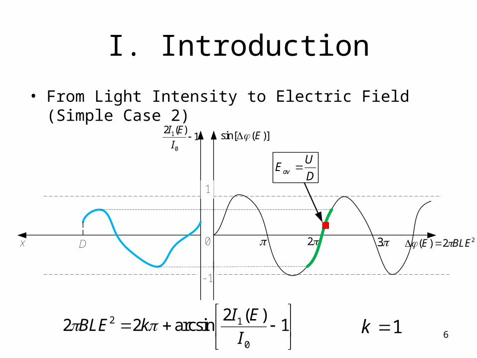
I. Introduction

• From Light Intensity to Electric Field (Simple Case 2)

22)( BLEE

)](sin[ E

2 3

1)(2

0

1 I

EI

0D

1

-1

D

UEav

x

1

)(2arcsin22

0

12

I

EIkBLE 1k 6

I. Introduction

• From Light Intensity to Electric Field (Complex Example)

22)( BLEE

)](sin[ E

2 3

1)(2

0

1 I

EI

0D

1

-1

D

UEav

Gap Spacing

1x2x

Possibility 1 Possibility 2

Possibility 1 Possibility 2

There are 4 possibilities for E in total

7

I. Introduction

• From Light Intensity to Electric Field (General Method):• Suppose there are N sections in the light intensity profile

and M monotonic sections of the sine function, the total number of possibilities is ;

• Then, enumerate all these possibilities, and find solution to the following optimization problem:

NM

1

0

1

0

)(&

1)(2

)](sin[..

min

CxE

I

EIEts

EdxUD

8

I. Introduction• Detect Light Intensity by CCD Camera

Light PropagatingWindow of the Test Cell

Top Electrode (HV)

Bottom Electrode (Ground)

x

0

D=5 mm

Imaging Area288 mm

620 pixels

CCD Exposure Time: 10 μs

Propylene Carbonate212 /102~ VmB 65~r

9

I. Introduction

• Synchronization of waveforms

Delay 1 Delay 2

ManualTrigger

15V pulse to HV impulse generator

TTL high level to CCD camera

Channel 1: 15 V pulse to trigger Marx generator (at t=0); Channel 2: TTL high level signal to trigger CCD camera; Channel 3: HV pulse measured by the 5068:1 capacitive divider (its

duration is ~10 ms and the peak voltage ~18 kV appears at t=0.1 ms)

10

I. Introduction• Experimental Procedures:

• Before the application of the high voltage, the CCD camera is set to be in the internal-triggering kinetic mode. Take 50 subsequent images, in which each pixel corresponds to an electron count indicating the brightness. Compute the average of them as background.

• Then switch the CCD camera to external-triggering image mode and press the manual trigger button of the delay generator. High voltage pulse is generated; the waveform measured by the divider is recorded by the oscilloscope. After being triggered the CCD camera takes the signal.

• Cut off the high voltage supply, use the real-time mode of the CCD to monitor the liquid stabilization, wait about 10 minutes and start the next measurement.

11

0 0.2 0.4 0.6 0.8 10.7

0.8

0.9

1

1.1

1.2

1.3

1.4

1.5

1.6

x/D

ED

/U

0 0.2 0.4 0.6 0.8 10

0.5

1

x/D

I 1(E)/

I 0

10 20 30 40 50 60 70 80 90 100

10

20

30

Cu(#2) electrodes in propylene carbonate; Image taken at t=0.1 ms; CCD exposure time 10 μs;

U~25 kV; D=5 mm; L=0.127 m.

• An example:• Narrow lines and

small fluctuations may not be seen by naked eyes.

• The old “counting fringes” method is inaccurate:

a) Spatial resolution

b) Number of fringes

c) Contrast of light intensity

d) Diffusivity of pixels

e) Time synchronization

2. Results

12

0 0.2 0.4 0.6 0.8 10.8

0.9

1

1.1

1.2

1.3

1.4

1.5

1.6

x/D

ED

/U

p11n11p13n11p02n11p01n11p21n11+ -

01 – Ti; 02 – Cu (alloy 110); 04 – Brass (alloy 360); 11 – Al (alloy 6061, anodized); 13 – Al (alloy 7075); 21 – Stainless steel (alloy 304, brushed)

0 0.2 0.4 0.6 0.8 10.7

0.8

0.9

1

1.1

1.2

1.3

1.4

1.5

1.6

1.7

x/D

ED

/Up02n02p04n02p01n02p11n02p21n02

+ -

2. Results• More electrode combinations (heterocharge distribution)

13

0 0.2 0.4 0.6 0.8 10.7

0.75

0.8

0.85

0.9

0.95

1

1.05

1.1

1.15

1.2

x/D

ED

/U

p21n22p21n18p21n21p21n15

+ -

0 0.2 0.4 0.6 0.8 1

0.7

0.8

0.9

1

1.1

1.2

x/D

ED

/U

p22n22p24n22p27n22p25n22

+ -

15 – Steel (alloy 1018, nickel-coated); 18 – Steel (alloy 1018);21 – Stainless steel (alloy 304, brushed); 22 – Stainless steel (alloy 304); 24 – Stainless steel (alloy 316); 25 – Stainless steel (alloy 440C); 27 – Stainless steel (alloy 321);

2. Results• More electrode combinations (homocharge distribution)

14

2. Results

0 0.2 0.4 0.6 0.8 10.75

0.8

0.85

0.9

0.95

1

1.05

1.1

1.15

x/D

ED

/U

6.0 kV11.1 kV14.4 kV18.0 kV24.9 kV

0 0.2 0.4 0.6 0.8 10.75

0.8

0.85

0.9

0.95

1

1.05

1.1

1.15

x/D

ED

/U

6.0 kV11.1 kV14.4 kV18.0 kV24.9 kV

0 0.2 0.4 0.6 0.8 1-1.4

-1.3

-1.2

-1.1

-1

-0.9

-0.8

-0.7

-0.6

-0.5

x/D

ED

/U

5.9 kV10.8 kV13.9 kV17.3 kV23.5 kV

0 0.2 0.4 0.6 0.8 1-1.4

-1.3

-1.2

-1.1

-1

-0.9

-0.8

-0.7

-0.6

-0.5

x/D

ED

/U5.9 kV10.8 kV13.9 kV17.3 kV23.5 kV

Stainless Steel (#21) Electrodes; Various Peak VoltagesPositive Polarity Negative Polarity

15

3. ResultsStainless Steel (#21) Electrodes; Various Peak Voltage

Positive Polarity Negative Polarity

0 0.2 0.4 0.6 0.8 1-0.6

-0.4

-0.2

0

0.2

0.4

0.6

0.8

x/D

(C

/m3

)6.0 kV11.1 kV14.4 kV18.0 kV24.9 kV

0 0.2 0.4 0.6 0.8 1-0.7

-0.6

-0.5

-0.4

-0.3

-0.2

-0.1

0

x/D

(C

/m3

)

5.9 kV10.8 kV13.9 kV17.3 kV23.5 kV

5 10 15 20 25-0.6

-0.4

-0.2

0

0.2

0.4

0.6

0.8

U (kV)

(C

/m3

)

Top Electrode

Grounded Electrode

0 5 10 15 20 25-0.7

-0.6

-0.5

-0.4

-0.3

-0.2

-0.1

0

U (kV)

(C

/m3

)

Top ElectrodeGrounded Electrode

16

2. Results• Up to now, we have shown the results of: • 1). For various pairs of electrodes and the same peak HV value (25 kV),

measuring the distributions of electric field and space charge density in the gap at the same instant (peak HV);

• 2). For the same pair of electrodes (S-S #21) and various peak HV values (both polarities), measuring the distributions of electric field and space charge density in the gap at the same instant (peak HV);

• Stainless steel electrodes can realize homocharge distribution in propylene carbonate. It seems that only when a stainless steel electrode is stressed by a positive polarity high voltage, the “injection” at the anode supersedes the heterocharge distribution due to bulk dissociation, which, however, is not exactly an injection, since propylene carbonate is reactive with stainless steel generating particle layers on the anode.

• We also did the following work:• For the same pair of electrodes and the same peak HV value, we video

recorded the dynamics of the charge injection and transport.17

2. Results• Practical difficulties and solutions:• The shortest exposure time of the CCD camera is 10 μs. Due to its high spatial

resolution and sensitivity, the transfer of an image to memory is relatively slow, resulting in a frame rate of < 100 fps.

• The high voltage pulse duration is ~ 10 ms, requiring the frame rate >> 100 fps.

• Directly recording the dynamics seems impossible at the current stage. The solution is to repetitively apply the high-voltage pulses and take images with different delays at different times.

• In principle we can take images every 10 μs; however, the jitter of the Marx generator brings about uncertainties in the starting time of the HV pulse, causing variations in the waveform. At t=0, the 15 V trigger pulse is applied to the Marx generator, but the time it takes to initiate a HV pulse may vary from 1 to 50 μs. There are fluctuations in the HV pulse starting time during the first 0.1 ms after trigger, which makes the measurement on the rising-edge of the HV pulse inaccurate and inconclusive.

• In all cases, the peak appears at about t=0.1 ms, and images were taken every 0.5 ms from t=0.1 ms to t=10.1 ms.

18

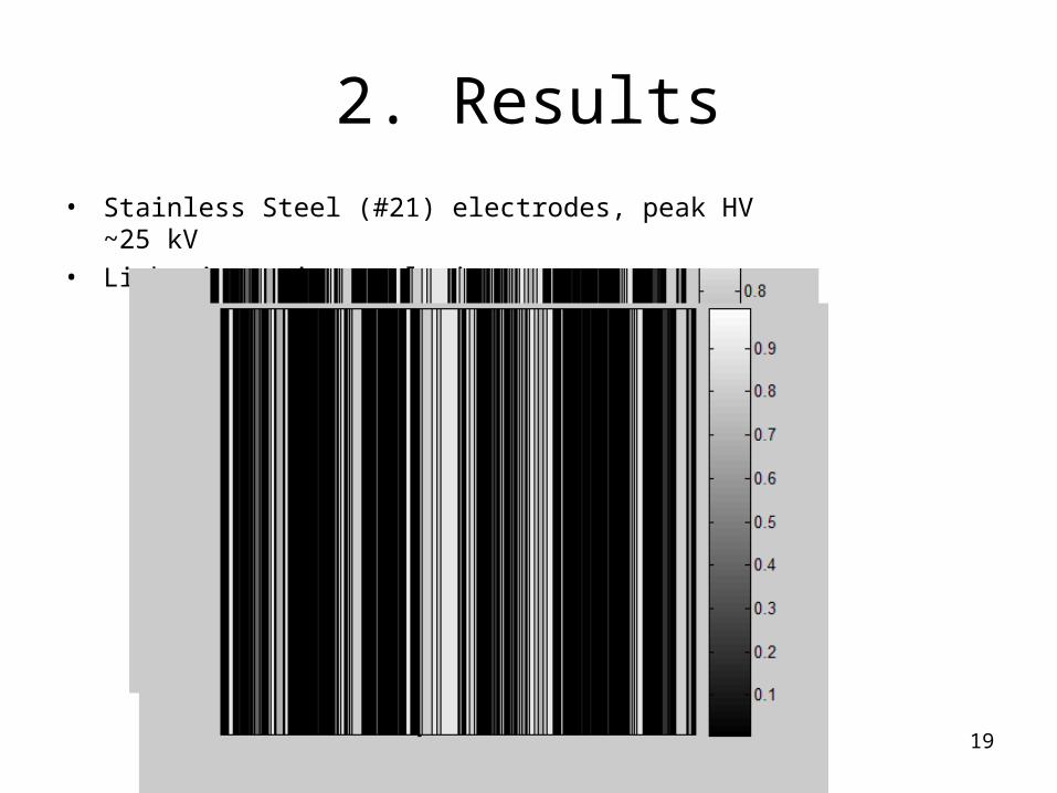
2. Results

• Stainless Steel (#21) electrodes, peak HV ~25 kV

• Light intensity evolution:

19

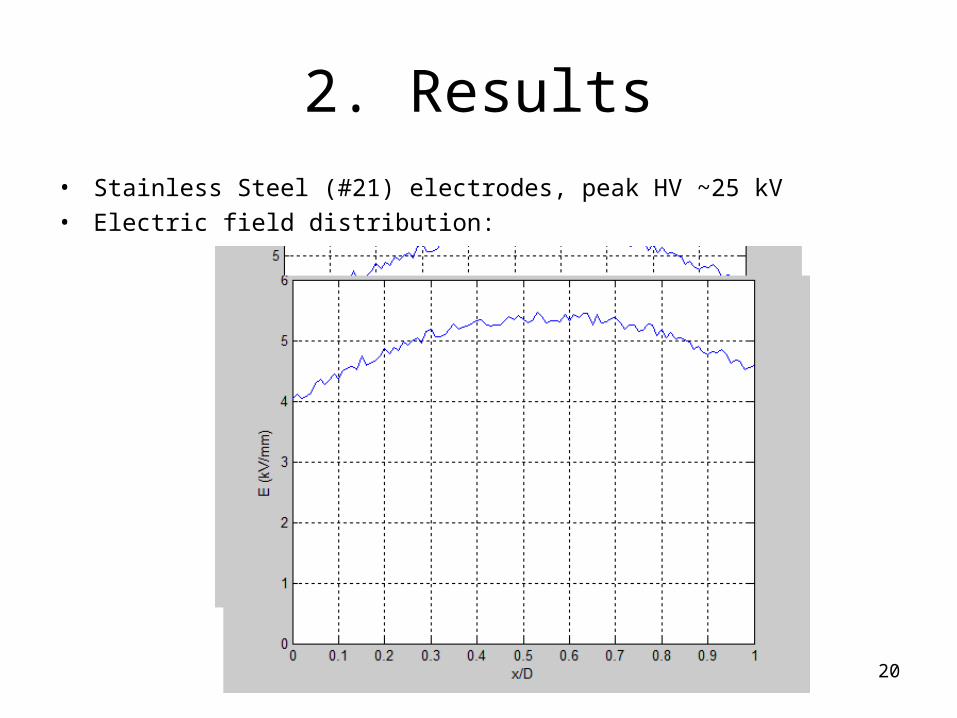
2. Results

• Stainless Steel (#21) electrodes, peak HV ~25 kV

• Electric field distribution:

20

2. Results

• Stainless Steel (#21) electrodes, peak HV ~25 kV

• Space charge dynamics:

21

Plan for Continuing Work

• Transformer oil electric field and charge density measurements for various electrode combinations and high voltages (March-May)

• Breakdown experiments to determine if there is a correlation between charge density magnitude and polarity near the electrodes and the breakdown voltage (June-August)

22

23