
MPRAMunich Personal RePEc Archive
Public and Private Investment in SaudiEconomy: Evidence from WeakExogeneity and Bound CointegrationTests
Hassan B. Ghassan
Umm Al-Qura University
4. February 2011
Online at http://mpra.ub.uni-muenchen.de/56537/MPRA Paper No. 56537, posted 18. June 2014 00:02 UTC

0
Public and Private Investment in Saudi Economy: Evidence
from Weak Exogeneity and Bound Cointegration Tests
Hassan Belkacem Ghassan1
Abstract
This paper investigates the long-run equilibrium relationship between the real private and
total public investment disaggregated into government and public enterprises investment in
Saudi Arabia by using the weak exogeneity and ARDL cointegration tests after using Engle-
Granger and Perron-Rodriguez cointegration tests. The results show the stable long-run
relation between private and total public investment. The public investment crowds out the
private investment, while this latter is crowding in by infrastructure government investment.
The absence of financial accelerator mechanism indicates that the private enterprises could be
in vicious loan-credit cycle. The finding indicate that long-run exceeds short-run crowding-
out, since the public sector still dominates the economic activities and attracts more capital
resources. But the disequilibrium of private investment is widely corrected and converges
back, with a high speed of adjustment, to its long-run equilibrium.
JEL classification: E22, C22
Keywords: Private Investment, Public Investment, Weak Exogeneity, Bound Cointegration,
Saudi Arabia.
1 Umm Al-Qura University, College of Economics and Islamic Finance, Department of Economics
Address: P.O. Box 175 Makkah 21955 Saudi Arabia. Phone: +00966-0125270000 Fax: +00966-0125531806
Email: [email protected] and [email protected]

1
1. Introduction
This article analyses the long and short run effects of total public investment on private
investment based on empirical data of KSA. Many papers examine the crowding effects using
an aggregated measure of public investment. The idea is to test these effects considering that
total public investment is decomposed into infrastructure government investment and
investment in public enterprises. The demand approach permits to evaluate the effect of
demand expectation (accelerator’s principle) and considers the user cost of capital (Jorgenson
1971) via the irreversible investment theory. The assumption of adjustment costs in the
investment process would appear to be more appropriate for modeling private investment
(Dixit & Pindyck 1994). We postulate that an adjustment process to the equilibrium
relationship exists between public and private investment. The reduction in private investment
is not only due to the uncertainty increasing but also to the public enterprises investment
crowding out effect. Nevertheless the infrastructure government investment would motivate
the private investment decisions.
Aschauer’s model, based on supply theory, concludes that infrastructure public investment
crowds in the private investment through the productivity effects of public capital (Aschauer
1989; Argimon et al. 1997). The public investment may crowd out private investment if the
additional government investment is financed locally by public bonds, which leads to an
increase in the interest rate, credit rationing and a tax burden for future generations (Rossiter
2002). This crowding effect could occur in the short run when the economy operates below
full employment level.
Based on the demand theory of investment, the hypothesis considered is that the effects of
public investment variations occur in short and long run (Aschauer 1989; Erenberg 1993;
Pereria 2001). To test these effects, the reduced-form private investment function is specified
assuming a logarithmic linear function. The ARDL cointegration leads to investigate the short
and long run relationship without imposing that the variables have the same order of
integration. This methodology seems to be more reliable in our empirical study. Many articles
do not verify hitherto a required condition of weak exogeneity test. The contribution of this
paper is to implement this test as a prerequisite in the bounds cointegration testing framework.

2
Many empirical evidence shows that there are mixed evidence of crowding out and
crowding in effects of public investment in developing countries (Atukeren 2005; Erden &
Holcombe 2006). The findings of Mitra (2006) for India using SVAR model suggest that
government investment crowds out private investment, though the government investment
had a positive impact on the economy in the long run. Chakraborty (2007) analyzes for India
the economic and financial crowding out through infrastructure and non-infrastructure
investments using VAR model. He exhibits that there is no evidence for economic crowding
out effect on private capital. The study of Looney (1992), based on the period 1960-1992,
indicates that there is no crowding effect between government and private investment. But
since1990s, the Saudi government measures enhance the investment environment and
promote the initiatives in private sector. It is expected in Saudi Arabia that the public
enterprises investment could crowd out the private investment, while the infrastructure
government investment would have a positive effect even if the government has a huge
budget for expenditures. Although the net effect of total public investment remains
ambiguous, so the result depends on which one of the two effects dominates.
This article is organized as follows; the second section describes theoretical backgrounds.
The economic reform process in Saudi Arabia is briefly presented in the third section. The
ARDL cointegration approach is treated in fourth section. The empirical results are exhibited
in the fifth section. The sixth section shows conclusions and policy recommendations.
2. The model of investment
There are two theoretical concepts of crowding out effect: economic and financial. The
economic effect occurs when the increase in public investment crowds out the private
investment through fiscal and economic policies, irrespective of the mode of financing the
fiscal deficit (Blinder & Solow 1973). The financial effect arises when the interest rate is
increased, because the public enterprises and government are borrowing heavily while the
private business and individuals encounter some restrictions loans. Using an augmented
accelerator model of investment (Wang 2005), the behavior of private investment can be
explained by the implicit reduced-form function f as follows:

3
rirCREYIBGIPUIPRfIPR ,,,,, *
1 with 01
IPR
IPR
IPU
IPR
≶0 0
IBG
IPR (1)
where the variables IPR, IPU, IBG, Y* and CRE design private investment, investment of
public enterprises, infrastructure government investment, expected demand (approximated by
real GDP) and credits to private sector, respectively. The variable rir shows a real interest rate
as a proxy of user cost of capital defined by ttt rLnrir 1/1 where tr and t denote
nominal interest rate and inflation rate, respectively (Neely & Rapach 2008). The positive
coefficient of lagged private investment reflects the irreversibility of investment. The total
public investment can have either a negative effect (substitution) or a positive effect
(complementarity) (Khan & Kumar 1997; Cruz & Teixeira 1999). So the infrastructure
government investment could reduce investment uncertainty in the private sector by tumbling
costs, raising productivity and increasing returns.
The flexible accelerator model suggests that the private investment is affected positively by
the expected demand. The effect of credits on private investment is expected to be positive.
Generally credit policies affect private investment via the stock of credits available to firms
that have access to preferential interest rates. If the real interest rate has a negative effect, this
endows with Jorgenson’s theory (1971). But a very small value of this effect would endow
with the theory of irreversible investment in conditions of macroeconomic uncertainty.
Bearing the above arguments in mind, the long run equation of private investment is
assumed to be given by the following natural logarithmic form:
(2)
where tu represents the error term which is an indicator for macroeconomic instability. The
elasticity parameters 2 and 3 are related to real crowding effect, while the parameter 6 is
more attached to financial crowding effect. The variables defined in Eq.2 with small letters
are the natural logarithmic of the variables defined with capital letters in Eq.1 except for the
variable rir which remains the same. If the relationship in Eq.2 is stable, that is, cointegrated
with appropriate adjustment, the crowding-out effect is checked (Shafik 1992; Ramirez 2000;
Ahmed & Miller 2000; Naqvi 2002). The assumption considered is that the adjustment would
be hold in short and long run following different processes of accelerator and cost of capital
ttttttt urircregdpibgipuipr 654321

4
effects. The adjustment mechanisms can be operated through the public investment and the
central bank. The former could be more or less rigid vis-à-vis the discrepancies and the latter
has different preferences regarding deviations from the long run equilibrium.
3. Economic reform process in Saudi Arabia
The government has established many public companies such Arab and American Company
of Oil (ARAMCO), Saudi Arabian Mining Company (MAADEN), Saudi Basic Industries
Corporation (SABIC) in petrochemical sectors, Saudi Electricity Company (SECO), Saline
Water Conversion Corporation (SWCC) and Saudi Telephone Company (STC). But to absorb
the burgeoning unemployed manpower, the government would stimulate the private sector
using a very moderate tax policy. The economic strategy is focused on the diversification of
income sources by developing non-oil sectors. It is expected that such sectors would generate
more job opportunities in the society improving incomes and enhancing the quality of life.
The private sector would expand progressively the role of national and foreign investors.
Also the banking sector has a substantial role to play by financing various economic activities
and providing more capital to investors. The financial private sector could attract Saudi
capital to flow back to the domestic and regional securities markets. The private sector role
could reduce the government debt burden on the public budget, and generate non-oil revenues
for the government budget (Table 1A). The development of a rather opened business
environment would rationalize the economic development and lead to increase the efficiency.
The Supreme Economic Council in 1999 (SEC) and the Saudi Arabian General Investment
Authority in 2000 (SAGIA) have been established to observe the performance of private
sector and eliminate at least the institutional barriers to investment such the abolition of local
sponsorship of foreign investors and the free capital flows.
During the 1990s, the Saudi government has planned to boost the private non oil sector. So
since 1990, the Saudi Arabia’s basic infrastructure was viewed as largely completed and
could support further private economic activities. Thus, the private investment expanded his
capacity of production and supported long run economic growth. The ratio of private
investment to GDP tended to increase, while the ratio of public investment decreased. Since
1998 the gap between private and public investment was persistently being reduced, but the
5
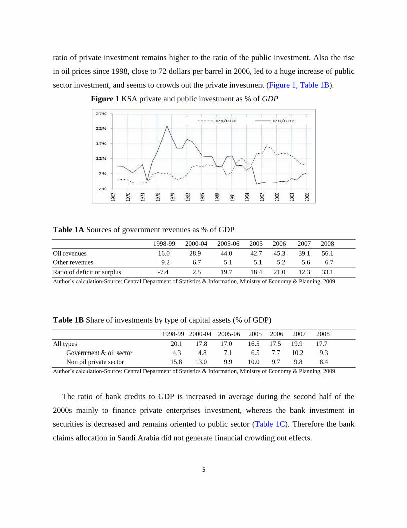
ratio of private investment remains higher to the ratio of the public investment. Also the rise
in oil prices since 1998, close to 72 dollars per barrel in 2006, led to a huge increase of public
sector investment, and seems to crowds out the private investment (Figure 1, Table 1B).
Figure 1 KSA private and public investment as % of GDP
Table 1A Sources of government revenues as % of GDP
1998-99 2000-04 2005-06 2005 2006 2007 2008
Oil revenues 16.0 28.9 44.0 42.7 45.3 39.1 56.1
Other revenues 9.2 6.7 5.1 5.1 5.2 5.6 6.7
Ratio of deficit or surplus -7.4 2.5 19.7 18.4 21.0 12.3 33.1
Author’s calculation-Source: Central Department of Statistics & Information, Ministry of Economy & Planning, 2009
Table 1B Share of investments by type of capital assets (% of GDP)
1998-99 2000-04 2005-06 2005 2006 2007 2008
All types 20.1 17.8 17.0 16.5 17.5 19.9 17.7
Government & oil sector 4.3 4.8 7.1 6.5 7.7 10.2 9.3
Non oil private sector 15.8 13.0 9.9 10.0 9.7 9.8 8.4
Author’s calculation-Source: Central Department of Statistics & Information, Ministry of Economy & Planning, 2009
The ratio of bank credits to GDP is increased in average during the second half of the
2000s mainly to finance private enterprises investment, whereas the bank investment in
securities is decreased and remains oriented to public sector (Table 1C). Therefore the bank
claims allocation in Saudi Arabia did not generate financial crowding out effects.

6
Table 1C Bank claims in Saudi Arabia (% of GDP)
1997-99 2000-04 2005-06 2005 2006 2007 2008
Bank investments in securities 16.8 18.8 11.2 12.1 10.3 11.5 13.2
Public sector 15.6 17.6 10.0 10.8 9.2 10.0 12.0
Private sector 1.2 1.2 1.2 1.3 1.0 1.4 1.2
Bank credits 28.1 29.6 37.7 38.3 37.2 41.4 42.5
Public sector 3.4 2.3 2.6 2.7 2.6 2.6 1.8
Private sector 24.8 27.3 35.1 35.6 34.6 38.8 40.6
Author’s calculation-Source: SAMA Annual Economic Reports and Bulletins 44, 2009
4. ARDL cointegration test
The most commonly used methods for conducting cointegration test include the residual
based on Engle-Granger test with single equation (1987), the maximum likelihood based on
Johansen-Juselius (1990) and Johansen test with multivariate VAR model (1992, 1995). The
existence of any long-run relation among a vector tttt xxyz 21 ,, of variables can be tested
by the ARDL or bound testing cointegration procedure. The main advantage of ARDL
modeling lies in its flexibility. Firstly, the variables can have different order of integration.
Secondly, the model takes sufficient lags to capture the Data Generating Process (DGP) in
General-To-Specific (GETS) modeling approach. Thirdly, the ECM, which integrates short-
run dynamics and long-run equilibrium, can be derived from ARDL through a simple linear
transformation (Banerjee et al. 1993). The ARDL approach uses the following unrestricted
Vector Error Correction Model (VECM) (Pesaran-Shin 1999; Pesaran-Shin-Smith 2001):
t
p
iititt zzcz
1
110 (3)
called equilibrium correction model, where 0c is the drift, and contain the long-run
multipliers and short-run dynamic coefficients, respectively. The matrix has a reduced
rank and can be decomposed as where and are matrices containing speed of
adjustments towards equilibrium and cointegration vectors, respectively. The vector of errors
is assumed to be identically distributed: ;0~ IDt where is positive definite. By
assuming conformable partitionings of relevant variables, vectors and matrices as:

7
t
t
tx
yz ,
xxxy
yxyy
x
yπ
,
x
y
,
i
i
x
y
i
,
t
t
x
y
t
,
xxxy
yxyy
if 0x (or 0xy and 0xx ), then tx is weakly exogenous for the parameters yxyy ,
and valid inference can be implemented in the conditional model of ty given tx and the past
of appropriate variables (Case III, unrestricted intercept and no trend in Pesaran et al. 2001):
tt
p
i
itityxtyyt uxzxycy
1
1
110 (4a)
tt
p
i
itityt uxzzcy
1
1
10 (4b)
called conditional or partial model, where xyxx 1 , ii xyi ,
tt xxxyxytu 1: (Johansen 1995, Pesaran et al. 2001 and Jacobs & Wallis 2010).
Assuming that a unique long-run relationship exists between the variables and tx is weakly
exogenous, the conditional VEC Model from (3) can be written as an ARDL model:
t
q
iiti
q
iiti
p
iititttt uxxyxxycy
21
0,23
0,12
111,231,121101 (4c)
with 11 . The disturbances tu are supposed uncorrelated. By construction tx are no
correlated to tu , and due to the unrestricted nature of the lag distribution of Eq.(4c), this
equation is identified and will be estimated consistently by least square method. Pesaran and
Shin (1999) suggest using a more parsimonious specification with ARDL approach.
Three main steps are required to implement the Bounds Testing Procedure. For
convenience, these steps are stated with selecting the order of the VAR (using AIC and BIC
criteria) and testing for weak exogeneity. The first step consists to estimate the Eq.(4c) in
order to test for the existence of long-run relationship among specified variables. This test is
realized by calculating a standard F-test for the joint significance of the lagged levels of the
variables: 0: 3210 H against 0: 3211 H . When a long-run relationship
exists between the variables in Eq.(4c), the F-test indicates which variable should be
normalized. The normalization gives the statistic xyFy / where y is the dependant
variable. Following Pesaran et al. (2001), the F test has a non-standard distribution; they

8
provide two asymptotic critical values bounds to testing for cointegration when the
explanatory variables are different order of integration I(1) and I(0).2 When the cointegration
is confirmed involving the stationary of estimated error te , the second step consists to
estimate the following level relationship defined by long-run ARDL 21 ,, qqp sub-model:
ty
q
i
iti
q
i
iti
p
i
itit xxycy
21
0
,23
0
,12
1
101 (5)
where ji represents the conditional long-run multiplier. This conditional ARDL equation
involves selecting the optimal orders of p and q by using AIC or SIC criterion. With the
annual data, the maximum number of lags is expected to be inferior or equal to 2. With the
lagged error-correction term tytect :1 , deduced from Eq.(5), the final step consists to
obtain the short-run dynamic coefficients from ECM as following:
tyt
q
i
iti
q
i
iti
p
i
itit ectxxyy
1
0
,23
0
,12
1
1
21
(6)
where iii 321 ,, are the short-run dynamic coefficients and is the speed of adjustment to
the long-run equilibrium.
5. Data and results
5.1 Data and unit root tests
The annual data are from 1968 to 2006 and extracted from the annual reports of Saudi Arabia
Monetary Agency (SAMA, report 43, 2007). The national accounts statistics break down the
Gross Fixed Capital Formation (GFCF) into private (IPR) and public investment (IPU)
realized by state-owned enterprises, each one includes local and foreign investment. The
infrastructure investment (IBG) is from government budget. The Data on real GDP are
calculated straightforwardly by implicit GDP deflator (base 1999). All data are taken in real
terms (1999 prices) with the appropriate deflators and they are not seasonally adjusted. A plot
of the variables over time indicates the presence of trend in the variables.
2 A lower value of F-statistic assumes that the variable is I(0) and its upper value supposes that the variable is
I(1). If F-statistic is above the upper critical value, then the null hypothesis of no cointegration could be rejected.
This null hypothesis could be accepted if the F-statistic is below the lower critical value.

9
The Dickey-Fuller Generalized Least Square (DF-GLS) de-trending test proposed by
Elliott et al. (1996) and the Ng-Perron test (MZ-GLS) following Ng & Perron (2001) have
been implemented for their reliability in small samples and less sensitivity to the lag choice.
They use a modified information criteria (MIC) which takes into account the fact that the bias
in the sum of the autoregressive coefficients is highly dependent on lags number. The results
(Table 2) of ADF-GLS and MZ-GLS unit root tests for the null hypothesis I(1) indicate mixed
order of integration, so the first difference of the variables ipr, cre, rir reject the unit root
hypothesis at 1%, while this latter is accepted for ipu, ibg and gdp. To check for possible size
distortions for ADF-type tests, we chose the lag order employing the data dependent method
(top-down testing) proposed by Ng & Perron (1995). The two unit root tests show mix I(1)
and I(0) variables, these results have significant implications for the cointegration analysis
frame. Then the ARDL’s approach is more appropriate in our empirical work, and the long
run private investment Eq.(2) can be justified by using the bounds test approach.
Table 2 Unit root tests with only constant 3
ipr ipu ibg gdp cre rir GLSADF -4.249
** -1.780
* -2.211
* -2.065
* -4.209
** -3.113
**
GLS
MZ -16.301**
-4.906 -6.476† -6.874
† -16.212
** -37.658
**
5.2 Weak exogeneity test
The weak exogeneity assumptions influence the dynamic properties of the conditional VECM
i.e. Eq.(4) and must be tested in the full system framework (Johansen 1992). The government
investment ( tibg ) can be treated as an exogenous I(1) variable, so the infrastructure
investment is considered one of the economic policy instruments. Considering
ttttt rircregdpipux ,,, weakly exogenous, the parameters of the conditional Eq.(4) of
3
In all Tables of results **, *, † indicate significance at the 1%, 5% and 10%, respectively. The Akaike
Information Criterion (AIC) has better theoretical and empirical properties. In the ADF-GLS test: one-sided
(lower-tail) test of the null hypothesis that the variable is non-stationary; at 1%, 5% and 10% asymptotic critical
values equal -3.46, -2.91 and -2.59, respectively when the model includes a constant and trend ; and equal -2.58,
-1.98 and -1.62, respectively when the model includes only a constant (Rapach & Weber, 2004). For the
Modified Phillips-Perron test: one-sided (lower-tail) test of the null hypothesis that the variable is non-stationary;
at 1%, 5% and 10% asymptotic critical values equal -19.95, -17.30 and -11.16, respectively when the model
includes a constant and trend ; and equal -13.80, -8.10 and -5.70, respectively when the model includes only a
constant (Ng & Perron 2001).

10
tt ipry : can be meaningfully estimated independently to the marginal distribution of tx
(Johansen 1995; Pesaran & Shin & Smith 2001). Under the concept of Granger causality, the
block exogeneity Wald test is used to test whether all endogenous variables could be
considered as exogenous. From the underlying VAR model, the result 458.28)4(ˆ 2 with
P-value 05011 E-. indicates that all level variables are globally exogenous.
When 0 yx and 0xx , then tx is weakly exogenous for 1: yy and
32, ,: yxxyx in Eq.(4). Given that can be written as . Then, the test of
weak exogeneity consists to test restrictions of nullity on the matrix i.e. coefficients
associated to error correction terms (Johansen 1992, 1995; Brüggemann 2002).4 From an
unrestricted VAR, the matrix can be estimated using the Johansen’s method; the use of
standard likelihood ratio consists to test whether the restrictions implied by the reduced rank
of could be rejected. Assuming there is only one cointegrating relation in VEC model, to
test whether the endogenous variables are weakly exogenous with respect to the parameters of
VEC framework, the constraint 0x , with no other restrictions on the parameters, would be
tested by solving a modified eigenvalue problem as described in Johansen (1995). This
implies that efficient inference can be constructed on yy and xyx, in the conditional model
(4). The corresponding LR statistic is computed as follows:
r
i i
iLnTLR1 ˆ1
~1
where i~ and i are the calculated eigenvalues with and without restrictions, respectively.
The statistic LR is asymptotically distributed with df2 where df is the degree of
overidentification. The results in Table 3 show that public investment can be considered as
strong exogenous in Eq.(4), and the weak exogeneity to the system is rejected only for the real
interest rate.5 By using the Granger causality test in the VAR framework, the variables ipu
4 The exogeneity test gives more convenience and allows efficient inference on the cointegration coefficients in
partial model (Jacob & Wallis 2010). So, this latter gives some arguments for the interpretation of economic
implications in the short and long run. 5 Also, if tx is weakly exogenous and 1ty does not Granger-cause tx , then tx will be strongly exogenous.
11
and gdp seem to be strong exogenous for the parameters yy and yx in the conditional model
(4a), but the variable cre remains weak exogenous. These outcomes provide evidence for the
underlying economic theory that crowding-out effect could be tested in the ARDL
cointegration framework.
Table 3 Weak exogeneity tests via Likelihood Ratio
ipu gdp cre rir 2
1 2.0983 0.2341 0.6338 5.1816
P-value 0.1475 0.6285 0.4259 0.0228
5.3 Cointegration tests
The existence of the long-run relationship, between private and public investment, is tested
using different tests of cointegration Engle-Granger (1987), Perron-Rodriguez (2001) and
Pesaran-Shin-Smith (1999, 2001). We don’t apply the maximum likelihood approach of
Johansen-Juselius (1990), because the same order of integration is required. If this
equilibrium relationship holds, it would imply that fiscal and monetary policies could
influence fluctuations in private investment and flows of credit to private sector.
Each cointegration test includes constant and trend as deterministic components, so the
visualizing data do support this basic specification. For the estimation of tu (from Eq.4c), the
lag order is chosen by AIC and t-sig. This lag is selected appropriately to reduce residual
serial correlation and avoid over-parameterization of Eq.(4c), the lag structure test gives
2p . From two first columns of Table 4, the null hypothesis of no cointegration using the
ADF cointegration test cannot be rejected. Thus, there is no evidence of cointegration at the
5% significance level using conventional Engle & Granger ADF test (1987). Furthermore, we
employ the Perron & Rodriguez (2001) cointegration tests with good size and power. The null
hypothesis of no cointegration is rejected at 5%. The contrast between the results in Table 4
suggests that the rejection using EG test entails a Type II error.

12
Table 4 Cointegration tests (dependent variable: ipr) 6
EG PR=EG
GLS
AIC t-sig AIC t-sig
-0.0758
(-1.513)
-0.0708
(-1.515)
-0.5043*
(-3.015)
-0.6769*
(-3.123)
Considering in the underlying VAR model the lag values from 1 to 2 of p and q for each
Eq.(4c), so 729612 regressions can be running using Microfit 5.0 (Pesaran & Pesaran
2009), the specification that minimize the AIC value is chosen. The bound cointegration test
is based on F-statistic which distribution under the null hypothesis depends on the integration
order of variables in Eq.(4c) and lag choice of order p . The critical value bounds are
computed by stochastic simulations using 2000 replications implemented in Microfit. If all
variables are I(0), the bootstrapping critical value at 5% is 2.98, and if they are I(1), the
critical value is 4.39. For cases in which some series are I(0) and others are I(1), the
bootstrapping critical value falls in the interval [2.98; 4.39].
Table 5A Bounds cointegration tests from Eq.(4c) ipr ipu ibg gdp cre rir
F (./X) 8.906**
1.131 1.555 3.731 0.849 2.421
The Eq.(4c) postulates that the crowding effects exist in short and long run. The bounds
cointegration test clearly rejects at 5% the null hypothesis of no cointegration for the private
investment equation (Table 5A). This result implies long-run cointegration relationship
amongst the variables when the regression is normalized on private investment. For gdp
equation, the test is inconclusive because the F-value falls within the bounds.
The bound cointegration test needs to be checked by usual diagnostic tests.7 The results
show that the models haven’t serial correlation and heteroskedasticity except for rir model
6 In EG’s test: one-sided (lower-tail) test of the null hypothesis that the variables are not cointegrated; at the 1%,
5% and 10% asymptotic critical values equal -4.02, -3.40 and -3.09, respectively (Rapach & Weber 2004). In the
PR’s test: one-sided (lower-tail) test of the null hypothesis that the variables are not cointegrated; at the 1%, 5%
and 10% asymptotic critical values equal -3.33, -2.76 and -2.47, respectively (Perron & Rodriguez 2001). 7 The diagnostic tests for ARDL model concern Lagrange Multiplier (LM) for the null hypothesis H0 of no
residual serial correlation, White Heteroscedasticity (WH) for H0 of no residual heteroskedasticity, Jarque-Bera
(JB) for H0 of residual normality and Ramsey’s RESET for H0 of no stable specification or no Functional Form
(FF) misspecification. In LM test, the lag length is 2 according to AIC for all variables except for ipu (lag=3).

13
(Table 5B). The ARDL model is robust against specification form except for rir model. All
models accept the null hypothesis of a normality distribution except the main model ipr which
has light leptokurtic distribution (Kurtosis=4.3). This can be attributed to a relative jump
component in the error term, which reflects news, events or information released by policy
government or private firms’ strategies.
Table 5B Diagnostic for Bounds cointegration tests (Eq.4c)
ipr ipu ibg gdp cre rir
LM
P-value
1.453
(0.26)
2.005
(0.15)
0.382
(0.69)
0.954
(0.40)
0.658
(0.53)
3.803
(0.04)
WH
P-value
0.400
(0.97)
2.166
(0.10)
0.606
(0.85)
1.256
(0.37)
1.896
(0.13)
3.890
(0.02)
JB
P-value
10.441
(0.01)
1.435
(0.49)
2.907
(0.23)
1.131
(0.57)
4.215
(0.12)
0.158
(0.92)
FF2
P-value
2.003
(0.16)
1.078
(0.36)
1.290
(0.30)
0.859
(0.44)
1.166
(0.33)
9.586
(0.001)
The existence of a long-run cointegration relationship allows to estimate Eq.(5) using the
ARDL(1,0,0,1,2,1) specification. Due to the difference in integration orders, the long-run
ARDL relation exhibits complicated dynamics between the private investment and their main
determinants.8 To derive the long-run coefficients (Table 6), Eq.(5) is then re-parameterized
by normalization on ipr.
Table 6 ARDL long-run estimation of ipr (Eq.5)
1 ipu ibg gdp cre rir
Coefficient -17.385 -0.913 0.421 2.773 -0.241 -1.999
Std. Error 1.83 0.09 0.06 0.23 0.06 0.30
Prob. 0.0004 0.0005 0.01 0.0000 0.13 0.009
The finding indicate that public investment affects negatively and significantly the private
investment with a crowding-out coefficient -0.913, whereas the infrastructure government
investment improves its investment efforts with a crowding-in coefficient 0.421. Thus, the net
result indicates that a net crowding effect is estimated close to -0.492, and shows that total
8 This estimated conditional ECM equation has one of complex roots with modulus 0.4091; the complex root is
i 2777.03004.0 where 1i , which suggests the presence of cyclical real private investment process
that quickly converges towards the equilibrium target i.e. Eq.5.

14
public investment crowds out private investment. The crowding out effect is then moderated
because the government spending expands, through the multiplier-accelerator mechanism, the
private sector activities, and hence stimulates the private investment. Also the private
investment is affected significantly and positively by the real GDP as it is predicted, but the
normalization leads to an unusual high coefficient.
The crowding out effect is verified in Saudi Arabia economy, but it does not signify the
unavailability of capital. The Saudi financial sector does not suffer from shortage of funds,
but in the long run there is some mismatching between fund needs of private enterprises and
loanable funds of banks. The no fixed maturity and no fixed financing cost could reduce these
mismatch problems. Also, this dilemma in crowding out effect could be explained by the fact
that local international banks encourage abroad investments and securities in international
markets. The international market affects domestic banking markets by attracting the Saudi
liquidity and reduces the loanable funds available for local investors (Claessens et al. 2001).
However, the credits to private sector have an insignificant negative coefficient at 5% level
in short and long run. In such case the private enterprises could be in vicious loan-credit cycle
named a financial accelerator, and the credit flows do not exhibit a positive role in private
investment process (Bernanke et al. 1999). The real interest rate still is a strong constraint to
the private investments in short and long run. Two arguments could explain this result,
inversely to public sector the private sector prefers largely external to internal finance (Table
1C), and the policy rate reacts to the real loan-credit cycle by increasing nominal interest rate.
These findings exhibit the absence of financial accelerator mechanism, but it remains that the
increase of external finance premium reduces the private investment.
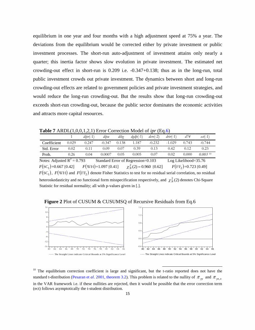
The results of Eq.6 indicate the absence of any instability of the coefficients.9 Figure 2
exhibits that both the associated cumulative sum and the cumulative sum of squares of
recursive residuals plots lie within the 5% critical bounds. The significant coefficient of error
correction term indicates that the disequilibrium is widely corrected and converges back to the
9 The regression of Eq.6 fits reasonably well and passes the diagnostic tests against misspecification,
heteroskedasticity, serial correlation and non normal errors. These tests could have lower power mainly against
important breaks. Overall, the conditional ECM of private investment growth equation has a number of desirable
features. The shift in the trend occurring at 1974 accounts a structural break due to unexpected growth of oil
revenues.
15
equilibrium in one year and four months with a high adjustment speed at 75% a year. The
deviations from the equilibrium would be corrected either by private investment or public
investment processes. The short-run auto-adjustment of investment attains only nearly a
quarter; this inertia factor shows slow evolution in private investment. The estimated net
crowding-out effect in short-run is 0.209 i.e. -0.347+0.138; thus as in the long-run, total
public investment crowds out private investment. The dynamics between short and long-run
crowding-out effects are related to government policies and private investment strategies, and
would reduce the long-run crowding-out. But the results show that long-run crowding-out
exceeds short-run crowding-out, because the public sector dominates the economic activities
and attracts more capital resources.
Table 7 ARDL(1,0,0,1,2,1) Error Correction Model of ipr (Eq.6)
1 dipr(-1) dipu dibg dgdp(-1) dcre(-2) drir(-1) d74 ect(-1)
Coefficient 0.029 0.247 -0.347 0.138 1.187 -0.232 -1.029 0.743 -0.744
Std. Error 0.02 0.11 0.09 0.07 0.39 0.13 0.42 0.12 0.23
Prob. 0.26 0.04 0.0007 0.05 0.005 0.07 0.02 0.000 0.003 10
Notes: Adjusted R2 = 0.793 Standard Error of Regression=0.103 Log Likelihood=35.76
1SCF =0.667 [0.42] WHF =1.097 [0.41] 960.0)2(2 N [0.62] 2FFF =0.723 [0.49]
1SCF , WHF and 2FFF denote Fisher Statistics to test for no residual serial correlation, no residual
heteroskedasticity and no functional form misspecification respectively, and )2(2N denotes Chi-Square
Statistic for residual normality; all with p-values given in [.].
Figure 2 Plot of CUSUM & CUSUMSQ of Recursive Residuals from Eq.6
-16
-12
-8
-4
0
4
8
12
16
80 82 84 86 88 90 92 94 96 98 00 02 04 06
The Straight Lines indicate Critical Bounds at 5% Significance Level
-0.4
0.0
0.4
0.8
1.2
1.6
80 82 84 86 88 90 92 94 96 98 00 02 04 06
The Straight Lines indicate Critical Bounds at 5% Significance Level
10
The equilibrium correction coefficient is large and significant, but the t-ratio reported does not have the
standard t-distribution (Pesaran et al. 2001, theorem 3.2). This problem is related to the nullity of yy and xyx,
in the VAR framework i.e. if these nullities are rejected, then it would be possible that the error correction term
(ect) follows asymptotically the t-student distribution.

16
6. Conclusions
This paper founds some evidence that private investment, public investment, GDP, credits to
private sector and real interest rate are bound together in the long-run. The finding shows that
public enterprises investment crowds out private investment in short and long-run. This
crowding out effect does not signify the unavailability of capital, because the Saudi financial
sector does not suffer from shortage of funds. But there is some mismatching between fund
needs of private enterprises and loanable funds of banks. The private enterprises could be in
vicious loan-credit cycle indicating the absence of financial accelerator mechanism. The
results show that long-run crowding-out exceeds short-run crowding-out, because the public
sector dominates the economic activities and attracts more capital resources. The
disequilibrium due to a shock is widely corrected and converges back with a high speed of
adjustment to the equilibrium. The main policy recommendations are that the infrastructure
government investment would be a useful channel to boost private sector in Saudi Arabia. The
real interest rate, discouraging private investment efforts in short and long term, would be at
lower level by reducing nominal interest and inflation rates. Also, given negative effects of
internal or external shocks, the private sector should be assisted to sustain its contribution to
the economic growth. The government measures should break down the vicious loan-credit
cycle and expand the joint private local and foreign investment projects.
References
1. Ahmed, H., and SM. Miller. (2000). Crowding out and crowding in effects of the
components of Government expenditure. Contemporary Economic Policy 18(1), 124-133.
2. Argimon, I., Gonzalez-Paramo JM., and JM. Roldan. (1997). Evidence of public crowding
out from a panel of OECD countries. Applied Economics 29, 1001-1010.
3. Aschauer, DA. (1989). Does public capital crowd out private capital? Journal of Monetary
Economics 24, 171-188.
4. Atukeren, E. (2005). Interaction between public and private investment: evidences from
developing countries. Kyklos 58(3), 307-330.

17
5. Banerjee, A., Dolado J., Galbraith J., and D. Hendry. (1993). Co-integration, Error
correction, and the Econometric analysis of non-stationary Data. Oxford, Oxford
University Press.
6. Bernanke, BS., Gertler M., and S. Gilchcrist. (1999). The Financial accelerator in a
quantitative business cycle framework. In Handbook of Macroeconomics, 1342-1393.
Volume I. Taylor, J.B. and M. Woodford (Eds.) Amsterdam: Elsevier.
7. Brüggemann, R. (2002). On the Small Sample Properties of Weak Exogeneity Tests in
Cointegrated VAR Models. Humboldt Universitaet Berlin, Sonderforschungsbereich, 373.
8. Chakraborty, LS. (2007). Fiscal Deficit, Capital Formation, and Crowding out in India:
Evidence from an Asymmetric VAR Model. The Levy Economics Institute and National
Institute of Public Finance and Policy, Bard College, Working Paper, 518. India.
9. Claessens S., Demirguc-Kunt, A. and H. Huizinga (2001). How does foreign entry affect
domestic banking markets? Journal of Banking & Finance 25, 891-911.
10. Cruz, De Oliveira B., and JR. Teixeira. (1999). The Impact of Public Investment on
Private Investment in Brazil: 1947-1990. CEPAL Review 0(67), 75-84.
11. Dixit, AK., RS. Pindyck. (1994). Investment under Uncertainty. Princeton: Princeton
University Press, New Jersey.
12. Elliott, G., Rothenberg T., and J. Stock. (1996). Efficient tests for an autoregressive unit
root. Econometrica 64, 813-836.
13. Engle, RF., and CWJ. Granger. (1987). Cointegration and Error-correction:
Representation, Estimation and Testing. Econometrica 49, 251-276.
14. Erenberg, SJ. (1993). The Real Effects of Public Investment on Private Investment.
Applied Economics 23, 831-837.
15. Erden, L., and RG. Holcombe. (2005). The linkage between public and private
investment: A cointegration analysis of a panel of developing countries. Eastern
Economic Journal 32(3), 479-492.
16. Jacobs, JP., and KF. Wallis. (2010). Cointegration, long-run structural modeling and weak
exogeneity: two models of the UK economy. Journal of Econometrics 158, 108-116.

18
17. Johansen, S. (1995). Likelihood-based inference in cointegrated vector autoregressive
models. Oxford, Oxford University Press.
18. Johansen, S. (1992). Testing weak exogeneity and the order of cointegration in UK money
demand data. Journal of Policy Modeling 14(3), 313-334.
19. Johansen, S., and K. Juselius. (1990). Maximum Likelihood Estimation and Inference on
Cointegration-with Application to the Demand for Money. Oxford Bulletin of Economics
and Statistics 52, 169-210.
20. Jorgenson, DW. (1971). Econometric studies of investment behavior: A survey. Journal of
Economic Literature 9, 1111-1147.
21. Khan, M and MS. Kumar. (1997). Public and private investment and the growth process
in developing countries. Oxford Bulletin of Economics and Statistics 59(1), 69-88.
22. Looney, RE. (1992). Real or illusory growth in an oil-based economy: Government
expenditures and private sector investment in Saudi Arabia. World Development 20(9),
1367-1375.
23. Mitra, P. (2006). Has Government Investment Crowded out Private Investment in India?
American Economic Review, Papers and Proceedings 96(2), 337-341.
24. Naqvi, NH. (2002). Crowding-in or Crowding-out? Modeling the Relationship Between
Public and Private Fixed Capital Formation Using Cointegration Analysis: the Case of
Pakistan: 1964-2000. Pakistan Development Review 41(3), 255-276.
25. Neely, CJ., and DE. Rapach. (2008). Real Interest Rate Persistence: Evidence and
Implications. Federal Reserve Bank of St-Louis Review 90(6), 609-641.
26. Ng, S., and P. Perron. (2001). Lag Length selection and the construction of unit root tests
with good size and power. Econometrica 69(6), 1519-1554.
27. Ng, S., and P. Perron. (1995). Unit Root Tests in ARMA Models with Data-Dependent
Methods for the Selection of the Truncation Lag. Journal of the American Statistical
Association 90, 268-281.

19
28. Pereria, AM. (2001). On the Effects of Public Investment on Private Investment: What
Crowds in What? Public Finance Review 29, 3-25.
29. Perron, P., and G. Rodriguez. (2001). Residual based tests for cointegration with GLS
detrended data. Manuscript Boston University.
30. Pesaran, B. and MH. Pesaran. (2009). Times Series Econometrics: using Microfit 5.0.
Oxford University Press.
31. Pesaran, MH., Shin Y., and RJ. Smith. (2001). Bounds testing approaches to the analysis
of level relationships. Journal of Applied Econometrics 16(3), 289–326.
32. Pesaran, MH, and Y. Shin. (1999). An autoregressive distributed lag modeling approach
to cointegration analysis. In S. Strom, (ed.) Econometrics and Economic Theory in the
20th Century: The Ragnar Frisch Centennial Symposium, Cambridge University Press.
33. Ramirez, MD. (2000). The Impact of Public Investment on Private Investment Spending
in Latin America: 1980-1995. Atlantic Economic Journal 28(2), 210-225.
34. Rossiter, R. (2002). Structural Cointegration Analysis of Private and Public Investment.
International Journal of Business and Economic 1(1), 59–67.
35. Shafik, N. (1992). Modeling Private Investment in Egypt. Journal of Development
Economics 39(2), 263-277.
36. Wang, B. (2005). Effects of government expenditure on Private Investment: Canadian
empirical evidence. Empirical Economics 30, 493-504.


