MPRAMunich Personal RePEc Archive

Monetary Policy Evaluation in RealTime: Forward-Looking Taylor RulesWithout Forward-Looking Data

Alex Nikolsko-Rzhevskyy

19. October 2008

Online at http://mpra.ub.uni-muenchen.de/11352/MPRA Paper No. 11352, posted 3. November 2008 11:00 UTC

Monetary Policy Evaluation in Real Time: Forward-Looking

Taylor Rules without Forward-Looking Data∗

Alex Nikolsko–Rzhevskyy†

October 19, 2008

Abstract

There is widespread agreement that monetary policy should be evaluated by using forward-looking Taylor rules estimated with real-time data. For the case of the U.S., this analysis canbe performed using Greenbook data, but only through 2002. In countries outside the U.S.,central banks do not regularly release their forecasts to the public. I propose a methodologyfor conducting monetary policy evaluation in real-time when forward-looking real-time datais unavailable. I then implement this methodology and estimate the resultant Taylor rulesfor the U.S., Canada, the U.K., and Germany. The methodology consists of calibratingmodels to closely replicate Greenbook forecasts, and then applying them to internationalreal-time datasets. The results show that the U.S. output gap series is well described byquadratic detrending, while Greenbook inflation forecasts can be closely replicated usingBayesian model averaging over Autoregressive Distributed Lag models in inflation and theGDP growth rate. German and U.S. Taylor rules are characterized by inflation coefficientsincreasing with the forecast horizon and a positive output gap response. The U.K. andCanada interest rate reaction functions achieve maximum inflation response at middle-termhorizons of about 1/2 year and the output gap coefficient enters the reaction functionsinsignificantly. Estimating the U.K. and Canadian Taylor rules as forward-looking is crucial,as backward-looking specifications produce nonsensical estimates. This is not the case forthe U.S. and Germany.

JEL Classification: E58, E52, C53Keywords: real-time data, Taylor rule, monetary rules, inflation forecasts, output gap.

∗ I thank Dean Croushore, Adriana Fernandez, Chris Murray, Tanya Molodtsova, Simon van Norden, DavidPapell, Elena Pesavento, Jeremy Piger, Tara Sinclair, and participants at presentations at the 17th MidwestEconometrics Group Meeting, Fordham University, and Emory University for helpful comments and discussions.I am thankful to Athanasios Orphanides for providing his data.† Correspondence: Department of Economics, University of Memphis, Memphis, TN 38152. Tel.: (832) 858-

2187. Email: alex.rzhevskyy@ gmail.com. Web: www.nikolsko-rzhevskyy.com

1 Introduction

During the last decade, simple policy rules have gained increasing popularity as a standard

way to monitor and evaluate behavior of central banks. This research was originated by Taylor

(1993) who showed that actual monetary policy in the U.S. could be well described by a simple

linear function of the inflation rate and a measure of economic activity.

Two important modifications of the original Taylor rule have received wide acceptance.

First, Clarida, Gali, and Gertler (1998) departed from the original backward-looking Taylor rule

to a forward-looking specification, which arguably better represents the objectives of central

banks. In order to control for inflation, the policy instrument would respond to the deviation

of the inflation forecast from its assumed target.1 Second, Orphanides (1999, 2000, 2003)

stressed the importance of policy rules being operational by showing that there are significant

differences between monetary policy evaluated over revised data and over real-time data – the

data available to policymakers at the time they were making their decisions. This research was

further expanded by the work of Croushore and Stark (2001), who collected and made publicly

available a real-time dataset for the U.S. It has by now become common practice to evaluate

monetary policy for the U.S. based only on real-time data.

For the case of the U.S., real-time forward-looking policy analysis can be performed using

the data available in the Greenbook, which contains inflation and output gap forecasts known to

the FOMC in real time. The Greenbook, however, is made publicly available with a five year lag,

which makes policy analysis after 2002 problematic. In countries outside the U.S., central banks

do not regularly release their forecasts to the public and real-time estimates of the output gap

are not typically available. The lack of appropriate data is one of the main reasons why research

on forward-looking central banks’ Taylor rules with real-time data has not been extended past

the U.S. to include other countries.

In this paper, I propose a methodology for conducting monetary policy evaluation in real-

time when forward-looking real-time data is unavailable. I then implement this methodology

and estimate the resultant Taylor rules for the U.S. (including the 2002–2007 period) and three

1Approximate and sometimes exact forms of this rule are optimal under the assumption that a central bankhas a quadratic loss function over inflation and output deviations from the long run trend (see Svensson (1999)among others).

1

other countries: Canada, the U.K., and Germany. The methodology consists of four steps. First,

I search for a model or a set of models which most closely reconstructs the Greenbook forecasts

for the U.S. I evaluate the models based on their ability to replicate the Fed’s out-of-sample

inflation forecasts and output gap estimates. Second, I apply the best model to construct what

U.S. Greenbook projections would have been for the last five years, for which the Greenbook is

not yet publicly available, if the Fed had used these models to produce their forecasts. Third,

I construct forecasts for the Bank of Canada, Bundesbank, and Bank of England using the

same models that produced the best forecasts of inflation and output gap for the U.S.2 While

using existing real-time datasets for the U.S. and Germany, I extend the existing U.K. dataset

beyond 2001 and assemble a new real-time dataset for Canada. Finally, after constructing

inflation forecasts and output gap estimates, I estimate forward-looking monetary policy reaction

functions for all four central banks.

Monetary policy evaluation results show that the U.S. post-2002 monetary policy closely

resembles pre-2002 one, where actual Greenbook data is available for estimation. The Taylor

rule estimated over the entire sample appears to be forward-looking, characterized with a high

inflation response coefficient that increases with the forecast horizon. The output gap coefficient

is marginally significant in each specification, and its value is close to Taylor’s (1993) postu-

lated value. As we increase the forecast horizon, interest rate smoothing significantly decreases,

which indicates that its typical estimate from a “backward-looking” regression might be biased

upwards.

German monetary policy reveals strong parallels with U.S. policy. It is characterized by

forward-looking behavior, with the inflation coefficient increasing with the forecast horizon, and

a positive and significant output gap response. The German output gap coefficient, however,

appears to be significantly higher than that of the U.S. Furthermore, evidence shows that the

Bundesbank also targeted the USD/DM real exchange rate. Unlike the U.S. and Germany,

the U.K. and Canada interest rate reaction functions achieve a maximum inflation response

at middle-term forecast horizons of about 1/2 year. Both monetary rules are characterized

by small and insignificant output gap coefficients. Estimating Taylor rules for the U.K. and

2I do not restrict the coefficients to be the same across countries and, therefore, reestimate the model forCanada, Germany, and the U.K.

2

Canada as forward-looking is crucial, since backward-looking specifications produce nonsensical

estimates. This is not the case for the U.S. and Germany. The forward looking specifications

are characterized by a higher than point-for-point inflation response coefficient for each out of

four countries, showing that the Fed, the Bank of Canada, the Bundesbank, and the Bank of

England obeyed the Taylor principle.

The plan of the remainder of the paper is as follows. In Section 2, I describe the model

to be estimated and provide an exposition of a non-linear Taylor rule. In Section 3, I outline

the empirical methodology used in my prediction experiment, and describe competing models

of inflation and output gap. Section 4 contains a description of the data used, and empirical

results are gathered in Section 5. Section 6 concludes.

2 The Model

The original Taylor (1993) monetary policy rule states that a central bank adjusts its short-

term nominal interest rate in response to changes in the inflation rate and the output gap.

Subsequently, forward-looking policy rules relating the interest rate to expected inflation and

the output gap have been found to be more successful than Taylor’s original backward-looking

specification (Orphanides (2003)). A specification of the Taylor rule that encompasses either

contemporaneous or forward-looking policy making would be:

i∗t = Eπt+h + δ(Eπt+h − π∗) + γyt +R∗ (1)

Here, i∗ is the short-term nominal interest rate target, π is the year-over-year inflation rate,

π∗ is the target level of inflation (usually treated as a constant 2 percent), y is the percentage

deviation of output from its long run trend (the output gap), and R∗ is the equilibrium level

of the real interest rate (also usually 2 percent). Following Clarida, Gali, and Gertler (1998), I

assume that the central bank adjusts actual interest rate, i, gradually towards its target level,

i∗, as it = (1− ρ)i∗t + ρit−1, where ρ is the smoothing parameter.

Even for the case of a contemporaneous Taylor rule with h = 0, neither right hand side

variable of Eq. 1 is observable in real time due to data collecting lags, and therefore expectations

of them need to be formed. If we treat π∗ and R∗ as being constant over time, we can combine

3

them into a single term c and, after allowing for additional policy determinants xt to affect

monetary decisions, the policy rule takes the following form:

it = ρit−1 + (1− ρ)c+ βE(πt+h|Ωt) + γE(yt|Ωt) + λE(xt|Ωt)+ et (2)

where Ωt = it, πt−1, yt−1, xt−1,Ωt−1 is the information set available to policymakers at time

t, and xt might include nominal and real exchange rates, the output gap growth rate, and the

foreign interest rate among other possibilities. To obtain an estimatable equation, Clarida,

Gali, and Gertler (1998), Gerberding, Worms, and Seitz (2005), and Davradakis and Taylor

(2006) eliminate unobserved forecasts from the expression by rewriting Eq. 2 in terms of realized

variables, implicitly treating the expectation sign E as being a rational expectation of the

future. There are three possible problems with this approach. First, realized values of inflation

are not available to policymakers in real-time and, therefore, are not part of the information

set. Second, using actual future values of inflation creates endogeneity, raising a problem of

finding good instruments. Finally, the realized values of inflation is the “effect” of the Fed’s

policy, not its “cause,” and therefore they should not enter the interest rate reaction function in

the first place. Indeed, suppose that both output and inflation are close to their target levels,

but the Greenbook forecast indicates that, conditional on current policy, we should expect an

increase in inflation up to 4% next year, while the policy objective is to keep it close to 2%.

Ceteris paribus, this increase in inflation expectations will induce the central bank to intervene

and raise interest rates now, which will result in actual inflation next year being close to the

targeted 2%. If we look at Fig. 1a, we see that after the Fed started targeting inflation in

the early 1980s, the Greenbook inflation forecast is typically above realized inflation when the

inflation rate is above its target level. This example illustrates a potential source of bias from

using realized values of inflation (2%) in the Taylor rule estimation versus the (never actually

realized) conditional forecast of 4%, which was in this example the actual driving force for the

Fed’s actions. Moreover, in the extreme case of perfect monetary control with forward-looking

objectives, realized values of inflation would always stay at their target level, and there would

be no relationship at all between them and the Central bank interest rate. Therefore, we need

to develop a way to construct real-time forecasts.

4

3 Methods

3.1 Output gap estimation.

In this section I define an appropriate measure of the output gap and develop a way to estimate

its value in each period E(yt|Ωt) given the real-time data available to policymakers in various

countries. Various measures are judged based on their ability to replicate Greenbook estimates

of the output gap.

One way to define the output gap is the difference between actual output and an unobserved

trend toward which output tends to revert. Given the limited availability of real-time data for

countries outside the United States, I adopt a univariate aggregate approach to estimate the

output gap, which requires only real GDP data; this approach is arguably the most common way

of measuring potential output (Taylor (1993), Clarida, Gali, and Gertler (1998), Taylor (1999),

Molodtsova, Nikolsko-Rzhevskyy, and Papell (2007) and many others use this method).3

There seems to be a consensus to use the latest available real-time data vintage to estimate

the output gap. Therefore, each output gap series uses exactly one vintage of GDP data, ensuring

that all values in the series are defined in the same way. Following the discussion above, I apply

six different detrending methods to the U.S. real GDP data:

1. Linear time trend. The (log of) real GDP yt is regressed on a constant term and a linear

time trend: X = 1 t, with coefficients estimated by OLS. The residuals from this

regression, scaled by 100, define the output gap, yt.

2. Quadratic time trend. The output gap is defined as deviations from a quadratic time

trend, similarly to the previous case, except X =1 t t2

. This detrending method is

often considered superior to linear detrending because it accounts for the U.S. productivity

slowdown in the 1970s. To add further flexibility to the trend and to improve its ability to

capture possible structural breaks, I use OLS and two other estimation methods. First, I

3The application of an alternative univariate NAIRU approach is limited due to its imprecise estimation.Staiger, Stock and Watson (1997) estimate the 95% confidence interval for the NAIRU to be 3 percentage pointswide. Mishkin (2007) describes in detail this and two other approaches: the production function approach andthe dynamic stochastic general equilibrium approach (DSGE). While use of the former is limited by the relativelysmall number of real-time variables available for countries outside the United States, the latter method requiresprecise knowledge of the structure of the U.S., U.K., German and Canadian economies. These problems makethe aggregate approach the only plausible choice.

5

use the rolling window estimation, where only last n values of GDP (instead of the entire

sample) are used for estimation. Second, I use the constant gain version of weighted least

squares, where past observations are discounted geometrically.

3. Band-pass filter. The filter isolates fluctuations in the data that persist for 1.5–8 years

(6–32 quarters). The filter and its properties are described in detail in Baxter and King

(1999). The symmetric nature of the filter creates an end-of-sample problem, which is

very relevant with real-time datasets. To cope with this issue I follow Watson (2007) by

using the AR(8) growth rate model to extend the log of real GDP series by 100 datapoints

in both directions before applying the filter.4 The gain is twosome: first, it allows me to

obtain a numeric value for the output gap at the end of the (initial) sample; second, it

allows me to increase substantially the moving average lag length K.5

4. Hodrick-Prescott (HP) detrending. The output gap series is derived by minimizing the

loss-function L =∑Tt=1 y

2t +λ

∑T−1t=2 [(τt+1 − τt)− (τt − τt−1)], where yt = yt−τt. Following

convention, I use λ = 1600. To account for end-of-sample distortions created by the filter,

I use a technique similar to the one described for the band-pass filter, making a backcast

and forecast of 12 observations before applying the filter. The same method is used in

Clausen and Meier (2005).

5. Unobserved Component (UC) model. The detrending mechanism is based on Clark (1987).

The model assumes that yt can be decomposed into unobserved non-stationary τt and

stationary ct, where τt is assumed to follow a random walk with drift, and ct is an invertible

ARMA(p, q) process. Additionally, Clark (1987) imposes a restriction of zero correlation

between trend and cycle innovations. This setup does not a priori impose any smoothness

in trend.

6. Beveridge-Nelson decomposition (B-N). This model is identical in the setup to UC model,

but it relaxes the assumption of zero correlation between trend and cycle innovations.

Instead, the correlation is estimated from the data; it appears to be close to −1, making

4Watson uses an AR(6) model to construct 300 forecasts of monthly data.5Before applying the filter, I modify the optimal filter weights, ah, as functions of the weights of the ideal

band-pass filter, bh, as ah = bh + θ, where θ = (1 −∑K

h=−K bh)/(2K + 1). I do this to impose a unity weightconstraint at the zero frequency.

6

the B-N decomposition more theoretically appealing than the UC model. See Morley,

Nelson, and Zivot (2003) for details.

I then compare estimates of the output gap series (yt−1|yt−1) from these different models

based on their ability to replicate the original real-time “Greenbook” estimates of the output

gap (yt−1|Ωt) used in Orphanides (2003); the series is available for 1969:1–1997:4.

3.2 Inflation forecasting.

My next step is to find a model that produces U.S. inflation forecasts as close as possible to

the Greenbook. I utilize modern inflation-forecasting models and techniques, expanding them

to estimate not only over the traditional “current-vintage” data, but also over “diagonals” and

“first-release” data6

The models I consider can be divided into three groups: simple univariate models, bivariate

models (usually in inflation and output growth), and atheoretical multivariate models. Whenever

possible, I enhance the original estimation techniques by allowing forecast aggregation for two

reasons. First, it is becoming recognized that aggregating forecasts over a set of models produces

RMSPE smaller then any single model in the set (Garratt, Koop, Mise, and Vahey (2007),

Marcellino, Stock, and Watson (2006), Rapach and Strauss (2007), and many others). Second,

anecdotal evidence shows that all central banks construct variety of models, each of which

produces a unique forecast.7 The forecasts are then combined (at least implicitly) into one

single number, based on subjective probabilities assigned to each model by banks’ officials.

Generally, I consider both the setup where the weights depend on the in-sample fit of the model

and on its out-of-sample performance.8

6If we define a value of a variable Xt at time k as it is though of in vintage v as xvk, then the ith lag of the variableXt is defined as this sequence of values: xt1−i, . . . , xtt−1−i, x

tt−i for “current vintage,” x1−i

1−i, . . . , xt−1−it−1−i, x

t−it−i

for “first releases,” and x11−i, . . . , x

t−1t−1−i, x

tt−i for “diagonals.” See Koenig, Dolmas, and Piger (2003) for details.

Table A-1 in Appendix provides an example. Corradi, Fernandez and Swanson (2007) postulate that “currentvintage” is arguably the data used by the Federal Reserve and other forecasters.

7The famous “Rivers of Blood” chart built by the Bank of England is a good example. See, for example, Wallis(1999).

8It is also worth noting is that the U.S. real-time dataset is much larger than the real-time datasets for othercountries – typically, U.S. data is available for a longer period and includes more real-time variables. Keeping inmind the ultimate goal of applying the best model to datasets for the United Kingdom, Canada, and Germany(which contain fewer variables), I utilize only a small subset of available real-time variables for the United States.This choice means that the forecasting results I obtain could possibly be improved by expanding the number ofvariables included, but if I did so the results would not be transferable to other countries.

7

The models I use are as follows:

1. A random walk (RW) model. This is a standard benchmark model used in most forecasting

exercises. If we define πt−1 to be the last available observation of inflation at time t,

then the RW model makes a no-change forecast of inflation for any horizon h as πt+h =

πt−1 + εt. Atkeson and Ohanian (2001) compare the RMSPE of Greenbook and random

walk forecasts of inflation, and find them very similar. However, Faust and Wright (2007)

replicate their study using an extended dataset, and show the superiority of the Greenbook

forecast.

2. Iterated autoregression (IAR). Another standard benchmark model is the AR(p) au-

toregressive model, where inflation πt is assumed to depend only on its past values:

πt = ρ0 +∑pj=1 ρjπt−j + εt. An h-period forecast is constructed by simply iterating

the 1-step ahead forecast. For “diagonals” and “first release” models I set p = 4, and for

the “current vintage” specification, I fix p = 8 since it appears to perform better.9 The

IAR model is also used as a benchmark model in Koenig, Dolmas, and Piger (2003).

3. Direct forecast from autoregression (DAR). This model is closely related to the IAR model

above, but in this model, each h-step ahead forecast is a simple 1-step ahead forecast from

an appropriate model: πt+h = ρ0 +∑pj=1 ρjπt−j + εt. Asymptotically, the IAR model

outperforms the direct AR if the IAR is correctly specified, but the direct forecast may

be more robust to possible misspecification (Marcellino, Stock and Watson (2006)). Or-

phanides and van Norden (2005) find that on average, autoregressive forecasts outperform

more complicated output-gap-based forecasts.

4. ARMA(1, 1). This framework models inflation as the sum of expected inflation and noise,

which fits the rational expectation framework: πt = ρ0 + ρ1πt−1 + ψ1εt−1 + εt. The

empirical motivation for this model comes from Ang, Bekaert, and Wei (2007) who show

that ARMA(1, 1) is often the best performing time series model for various measures of

inflation. Moreover, for the case of CPI inflation, it outperforms all Phillips curve and

9The same set up is used for other autoregressive models described below, unless otherwise noted. Estimationresults for uniform p = 4 and p = 8 are presented in Appendix in Tables A-4 and A-5, respectively. The appendixis available in pdf format for viewing or downloading at www.nikolsko-rzhevskyy.com.

8

term-structure models. The model is estimated by maximum likelihood, conditioning on

the assumption ε1 = 0. Inflation forecasts for various horizons h are computed recursively.

5. Constant gain CG-VAR(p). This model is similar to the best performing model in Branch

and Evans (2006), who use a low order constant gain VAR model in output growth gyt and

inflation πt to forecast inflation out of sample. If we define Yt = πt, gyt ′, εt = ε1t, ε2t′,

µ = µ1, µ2, and Φ as a 2 × 2 matrix of coefficients, then: Yt = µ +∑pi=1 ΦiYt−i +

εt. The model is recursively estimated under various assumptions about the influence of

additional observations on parameter estimates. The specification with common constant

gain significantly outperforms more complicated alternatives and also provides the best fit

with the Survey of Professional Forecasters data.10 To maximize performance of the model,

I consider CG-VAR with 4 different values of gain γ, where γ ∈ 0.025, 0.050, 0.075, 0.100.

6. Bayesian Phillips curve. This is the most successful bivariate model used in Orphanides

and van Norden (2005) and it enhances the DAR models (above) by adding lags of the

real output growth gyt not subject to any filtering. Using output growth in this way

can be interpreted as implicitly defining an estimated output gap as a one-sided filter of

output growth with weights based on the TOFU estimates (van Norden (1995), Orphanides

and van Norden (2005)): πit+h = ρ0 +∑pπij=1 ρjπt−j +

∑pgij=1 δjg

yt−j + εit. In contrast to

Orphanides and van Norden, I do not choose the optimal ADL lag lengths pπi and pgi

based on the Bayesian Information Criterion (BIC). Instead, I estimate m models for

every combination of pπi , pgi ∈ 1..p, and then average the forecasts using the Bayesian

model averaging (BMA) approach.11 Specifically, letting πit+h be a forecast of πt+h from

the ith model, the BMA forecast is πt+h =∑ni=1 ω

ti πit+h, with ωti being the posterior

model probabilities. Asymptotically, it can be shown that the logarithm of the marginal

likelihood of a model Mi is proportional to the Schwartz or BIC as logP (Data|Mi) ∼

logL − k log(T )2 . Under standard noninformative priors about model probabilities, the

10Constant gain is a version of weighted least squares, where past observations are discounted geometrically,meaning that each new observation has the same effect on parameter estimates as do past observations. Incontrast, traditional OLS employs a “decreasing gain” of t−1, and each new observation has an ever decreasingeffect on the parameter estimates.

11Garratt, Koop, Mise, and Vahey (2007) show that the best single BIC model never performs as well as acombined forecast. Nocetti and Smith (2006) show that BMA is the ex ante optimal way of forecasting in thepresence of model uncertainty.

9

exponent of BIC provides weights proportional to the posterior model probabilities used in

BMA, and maximum likelihood estimates (MLEs) can be used as point estimates. Garratt,

Koop, Mise, and Vahey (2007) provide additional details. A simplified equal averaging

version of this method with ωi = n−1 is successfully used in Bates and Granger (1969) and

Stock and Watson (2003).

7. Model clustering. This technique was first introduced by Aiolfi and Timmermann (2006).

The authors split the population of models into K clusters based on models’ performance

out of sample: Models with the lowest MSPE are assigned to the first cluster, those with

slightly worse performance fall in the second cluster, etc. The resulting forecast is the

weighted average of individual forecasts of the models from the first cluster. This method

works quite well in Rapach and Strauss (2007), who apply it to forecast housing prices.

Following them, I also use the C(K,PB) algorithm to average individual forecasts, but I

set the number of clusters K equal 5.12 The battery of models I consider is described as:

πit+h = ρ0 +∑pπij=1 ρjπt−j +

∑pgij=1 δjg

yt−j +

∑Jij=1 βjixjt+ εit. Here, xitni=1 is a collection of

potential predictors, including the unemployment rate ut, real output growth gyt , and the

output gap yt among others. Lag lengths pπi , pgi are allowed to vary between 1..4, and

Ji takes values from Jj = 0 (neither xj variable is included in the model), to Jj = n (all

xj variables are present).13 Individual forecasts are then combined into one aggregated

forecast. The crucial difference between this way of averaging, and the traditional BMA

is that with clustering, model weights are assigned based on out-of-sample performance of

the model, versus the in-sample fit with BMA.

8. Data-rich Bayesian model averaging. This model is the large dataset specification that

appears to be the only strong competitor to the Greenbook forecast of inflation considered

in Faust and Wright (2007): πit+h = ρ0 +∑pj=1 ρjπt−j +βixit + εit, where h = 0..5 is the

forecasting horizon, and xitni=1 is a collection of potential predictors. Faust and Wright

demonstrate that Bayesian averaging among all n models does a considerably better than

12I chose cluster size based on the following procedure. First, I split the sample into 2 parts, and for differentvalues of K = 2, 3, 4, 5, 6, I calibrated the model based on its performance over the first part of the sample.Then I tested it using the second part of the sample, and K = 5 performed the best.

13Thus, this specification embeds a univariate AR(p) model, the bivariate Phillips curve and VAR(p) models,and a number of atheoretical multivariate models.

10

any of the univariate inflation forecasts, and generally gives the smallest RMSPE among

all atheoretical inflation forecasts considered.

4 Real-time Datasets

4.1 U.S. dataset 1965:4–2007:1.

I use two different real-time datasets for the Untied States. The first comes from the Federal

Reserve Bank of Philadelphia, and it is described in detail in Croushore and Stark (2001).14

From the Core Variables/Quarterly Observations/Quarterly Vintages section, I extracted real

and nominal GNP/GDP and the unemployment rate, with vintages going back to 1965:Q4. (The

last vintage I use is 2007:Q1.) For every variable, the data in each vintage goes back to 1947:1,

and new values become available with a one-quarter lag. This means, for example, that for the

2000:Q1 vintage, the last available observation of the real GDP series is for 1999:4. The effective

Federal Funds Rate is never revised, and this data comes from the Federal Reserve Board of

Governors.15

I also use the Greenbook dataset, which is currently available up to 2001:4 (as of October,

2007).16 From this dataset, I use the annualized quarter-over-quarter growth rate forecast of

the GNP/GDP price level, which I transform into year-over-year growth rates by averaging 4

consequent inflation forecasts (some of which are actual realized values).17 This series and other

Taylor Rule variables are plotted at Fig. 1b and Fig. 1c.

4.2 Canadian dataset 1977:3–2007:1.

I assembled the real-time quarterly Canadian dataset using January, April, July, and October

issues of the Bank of Canada Review,18 because new updated GDP data is typically released for

the first time in these months. The first vintage in the dataset comes from the July 1977 issue

14http://www.phil.frb.org/econ/forecast/readow.html15http://www.federalreserve.gov/releases/H15/data/Monthly/H15 FF O.txt16http://www.philadelphiafed.org/econ/forecast/greenbook-data/index.cfm17For example, inflation at time t + 2 is the average of these quarter-over-quarter Greenbook entries: a t + 2

inflation forecast, a t+1 inflation forecast, a nowcast of inflation at time t, and the realized inflation at time t−1.18Since Winter 1996, the Bank of Canada Review has been published quarterly, and four issues are called

Winter, Spring, Summer and Autumn.

11

of the Review, and the last one is from Spring 2007. The variables included in the dataset are

(seasonally adjusted) nominal and real GNP/GDP, money M1/M1Gross (annualized quarter-

over-quarter growth rate), the unemployment rate, CPI all items, and Core CPI (over time, the

measure changes from CPI All Items minus Food to CPI All Items minus Food and Energy to

Core CPI). For real and nominal GDP, data in each vintage goes back to 1960:1. CPI All Items

data goes back to 1971:1, while the Core CPI, M1, and unemployment series start in 1972:2.

The data is typically updated with a four-month lag, meaning that, for example, in January

1988 the latest real GDP value was for 1987:3. (See Appendix for additional details.)

4.3 German dataset 1979:1–1999:1.

The real-time dataset for Germany was collected by Gerberding, Worms, and Seitz (2005). It

consists of real and nominal GDP/GNP, year-over-year CPI inflation, M1/M3 growth rates, the

Bundesbank money growth target and internal estimates of the potential output, which makes

calculation of the output gap trivial. For real and nominal GDP/GNP, the first available vintage

is 1974:Q1, with data going back to 1962:1. CPI vintages start in 1973:4, but typically only

5–8 observations are recorded (the earliest is 1972:4). Finally, money growth vintages begin in

1974:Q1, and the earliest observation is 1970:1. The official money growth targets series was

kindly shared by Gerberding, Worms, and Seitz. All variables are typically updated with a

one-quarter lag.

4.4 U.K. dataset 1983:3–2007:1

This dataset consists of (seasonally adjusted) real-time real GDP data, downloaded from the

Bank of England’s online real-time database, described in Egginton, Pick, and Vahey (2002),

and GDP deflator data, used in Garratt and Vahey (2006) and Garratt, Koop, Mise, and Vahey

(2007), which was kindly shared by the authors. The dataset contains a mixed frequency of

vintages for quarterly data; for consistency, I use only those vintages corresponding to the last

month in each quarter. The data is consistently available after September 1983, which I use as a

starting point in the dataset.19 The last recorded vintage in this dataset is March 2002, and for

19Due to data availability, I had to use July 1992, October 1992 and January 1993 vintages instead of June 1992,September 1992 and December 1992 vintages, respectively, which are missing from the dataset. GDP deflatordata contains vintages beginning in November, 1981. There are several reasons why I do not use earlier data.

12

most major revisions, long time series going back to 1955:1 are recorded. I extended the original

dataset to 2007:Q1 using the same source of data (the Office for National Statistics’ Economic

Trends.)

5 Empirics

5.1 Output gap estimation results.

Table 1 compares the in-sample performance of the detrending methods described in Sec-

tion 3.1. The primary measure of the goodness-of-fit is the Root Mean Square Prediction Error,

RMSPE =√

1T

∑Tt=1(yt − yt)2. Two other measures include the Sign statistics, which shows

how often a model matches the Greenbook’s booms and recessions, and a simple correlation be-

tween the two output gap series. The best performing model in terms of RMSPE is the rolling

window detrending, with a window size of 120 quarters (30 years). The strongest correlation

among all models is achieved using the constant gain estimation method with γ = 0.005. In that

case, 77% of variation in the Greenbook series is explained by the model. Quadratic detrending

is a clear winner among “traditional” detrending mechanisms, with a correlation of 0.87 and a

RMSPE of 3.651. Surprisingly, despite its popularity, the Hodrick-Prescott detrending method

is one of the worst at predicting the Greenbook estimates: besides having high MRSPE of 5.438,

it produces a gap of the same sign as the Greenbook only in slightly more than 50% of cases,

and it is virtually uncorrelated with the Greenbook series. The worst performing model is the

B-N decomposition, although this result is expected: B-N detrending is known to produce a

small and noisy cycle component. The rolling window detrending model with a window size of

80 quarters is among the best models, with a balanced performance in all three categories. In

light of these findings, I use the 20 year rolling window as the main method to construct the

output gap series for the United States, United Kingdom, and Canada.

First, neither of the monthly real GDP vintages I am interested in is available before September, 1983. Second,the data from the October 1981–July 1982 vintages is missing.

13

5.2 Inflation forecasting results.

This section details forecasting results of the inflation models, described in Section 3.2. Specifi-

cally, I concentrate on the extent to which different models and types of real-time data reproduce

conditional (Greenbook) and rational (actual data) forecasts of inflations. The best “Greenbook”

model is then used to reconstruct the forecasts for the United States and other countries.

The results, which summarize the relative ability of the forecasting models to replicate

Greenbook forecasts, are presented in Table 2. We see that averaging typically gives us the

smallest RMSPE (models (6) and (7)), and that the “current vintage” setup produces results

superior to both the “diagonals” and “first release” specifications. This result is consistent with

the hypothesis that the Fed uses the last available (in real-time) vintage of data to construct its

forecasts. Another interesting result is that a simple ARMA(1, 1) model performs exceptionally

well for long-term horizons. The “BMA Phillips curve” model (6) with “current vintage” data

has the most stable performance among all the models I consider.20 For the rest of the paper,

I use it as my main specification to construct inflation forecasts, as it appears to be the best

model to replicate the Greenbook conditional forecasts of U.S. inflation.21

For the United States, I combine the original Greenbook inflation forecast (before 2001:4)

and my conditional forecast (2002:1–2007:1) into a single series for each forecast horizon h and

use it for further estimation.

5.3 U.S. Monetary policy.

5.3.1 History of monetary policy

The inflation stabilization period in the United States started in August 1979 with the appoint-

ment of a new Federal Reserve Board Chairman Paul Volcker, who reduced inflation rates in

20Anecdotal evidence suggests that the Greenbook contains conditional forecasts of the economy at someperiods, and unconditional at the others, which raises a question of stability of the forecasting model. However,data shows that even if this is indeed the case, the different between the forecasts is minimal. To test this Isplit the whole sample into two parts, and reestimate all forecasting models for the second part of the Greenbooksample: 1987:2–2000:4. The results are very similar (Appendix, Table A-3), and RMSPE picks the same “currentvintage” BMA Phillips curve model as the best model to replicate Greenbook forecasts.

21I also investigate whether the model that best predicts the Greenbook forecasts will also be the model thatbest predicts actual inflation, and I find that the answer is no (Appendix, Table A-12). In fact, using “diagonals”and “first-release” typically produces smaller RMSPE than using “current vintage” data – a finding, similar toKoenig, Dolmas, and Piger (2003)

14

the U.S. from two-digit numbers in the 1970s to 7% in 1982:1, which I use as a starting point

in my estimation sample that runs through 2007:1.

Alan Greenspan replaced Paul Volcker in August 1987, and successfully kept inflation at

low levels throughout his chairmanship. Ability to control inflation is typically attributed by

researchers to adherence of the Taylor principle, which says that to maintain price stability,

a central bank should respond more than one-to-one to deviations of inflation from its target

level. Indeed, the Taylor’s (1993) original study analyzes Greenspan’s 1987:1–1992:3 period and

shows that the backward-looking Taylor Rule with an inflation response of 1.5 and an output

gap response of 0.5 fits the data remarkably well. Clarida, Gali, and Gertler (1998) estimate a

forward-looking Taylor rule over an extended 1979–1994 sample of monthly data, and find the

inflation coefficient in a baseline specification to be 1.79. The authors, however, use revised data

and realized future values of inflation in place of forecasts, which is subject to my critique.

Orphanides (2004) uses Greenbook forecasts to estimate forward-looking versions of the Tay-

lor rule over a similar time span (1979:3–1995:4) and finds the Fed to be forward-looking: its

inflation response appears to be always higher than one, and it increases as the forecast horizon

goes from 1 to 4 quarters hence. In his 2003 paper, Orphanides shows that the Taylor rule’s

fit can be improved if we add a growth targeting term to the baseline Eq. 2 specification. The

expected output gap growth E4yt+3 = Eyt+3 − yt−1 variable appears to be highly econometri-

cally significant in his 1982:3–1997:4 sample. The value of the expected inflation and expected

output gap growth coefficients are 2.73 and 2.68, respectively. Currently, no results are available

for 2002:1 and later periods due to the 5-year publication lag for the Greenbook.

I will start by verifying some of the results presented above. Then, I will estimate the forward

looking Taylor rule for several subsamples, including one with the last 5 years of data. I fix the

sample at 1982:1–2007:1.

5.3.2 Taylor rule estimation (U.S.)

I start with estimating the full sample (1982:1–2007:1) Taylor rule for different forecast horizons

h = 0..6, where h = 0 corresponds to observed (t−1|t) data. The policy variable is the Federal

Funds rate at the end of the quarter, giving the Fed time to respond to intra-quarter news. The

results are presented in Table 3.22

15

We see that the Fed shows strong pro-active behavior: when the forecast horizon increases,

the value of the inflation response coefficient, β, goes up, reaching a maximum of 2.84 (with a

standard error of 0.59) at h = 5. The goodness of fit measure, R2, also increases, indicating that

the forward-looking version of the Taylor rule fits data better than the backward-looking one.

Orphanides (2004) comes to the same conclusion using a 1979:3–1995:4 sample. The output

gap coefficient is marginally significant and its value is close to Taylor’s (1993) 0.5. Another

interesting observation is that the value of the smoothing coefficient ρ = 0.91 (with a standard

error of 0.05) for h = 0 is significantly overestimated compared to ρ = 0.82 (with a standard

error of 0.05) for h = 5. This shows that smoothing does occur, but at a smaller extent than we

would conclude in estimating the backward-looking version of the Taylor rule.23

My next step is to estimate the forward-looking version of the Taylor rule for two subsamples,

one falling on Paul Volcker’s chairmanship (1982:1–1987:1) and another on Alan Greenspan

and Ben Bernanke’s chairmanships (1987:2–2007:1).24 Besides standard Taylor rule variables

(inflation and output gap) I also include the output gap growth variable.25

The estimates, which reveal some differences and similarities between the two periods, are

presented in Table 4. First, the one-year-ahead inflation forecast response coefficient, β, is

statistically identical in both periods, and its size accords to full sample estimates; this result

is robust to inclusion of the output gap growth variable. Point estimates, though, are higher

in the earlier subperiod. Second, we see that interest rate smoothing increased considerably

from 1982–1987 to 1987–2007. Indeed, while ρ ≈ 0.26 for the former period, it reached 0.86

in the latter one. The difference is also evident in Fig. 1d. Third, the Fed seems to have paid

more attention to the output gap after 1987 than it did beforehand: the output gap coefficient

is positive and significant for 1987–2007, and insignificant for 1982–1987. Finally, the output

gap growth variable is significant in 1987–2007 subsample, but is not significant during Volcker’s

22To test the validity of inflation forecasts, I compare Taylor rule estimates with both artificial and originalGreenbook projections over the Greenbook sample (Table A-6 in Appendix). The difference between them isnever econometrically significant. The results also show that using realized values of inflation in place of real-timeforecasts might result in biased estimates.

23For discussion of other reasons why ρ might be overestimated, refer to Rudebusch (2006) and Lansing (2002).24Note that original Greenbook data is available for the entire 1982:1–1987:1 subsample.25That variable comes from two sources: The Greenbook series before 1997:4 is available in Orphanides (2003). I

combine it with the OECD estimates, which could be calculated using the semi-annual issues of OECD EconomicOutlook. Each issue contains past estimates and future forecasts of annual output gap values for all OECDcountries including the US. I obtain quarterly values from annual estimates using quadratic interpolation.

16

chairmanship. Nevertheless, the Taylor rule specification in each subperiod shows that monetary

policy was stabilizing, and the Taylor principle was obeyed.

5.4 Canadian Monetary policy.

5.4.1 History of monetary policy

The estimation sample starts in 1988:1, when the Bank of Canada governor, John Crow, deliv-

ered his Hanson Memorial Lecture at the University of Alberta, explicitly setting price stability

as the Bank’s primary objective, and runs through 2007:1. As Gordon Thiessen, another former

Bank of Canada governor, noted in 2000, “The Hanson lecture contained probably the strongest

commitment to price stability that had ever come from the Bank of Canada.” Following the

speech, in February 1991 the Bank of Canada officially announced the introduction of an in-

flation target. The acceptable range was set at 2–4 percent, with inflation measured by Core

CPI (inflation excluding food and energy).26 Thiessen (2000) defines the current stand of the

Canadian monetary policy as “directed towards a single long-run objective: the attainment

and maintenance of price stability.” During this relatively long history of inflation targeting,

inflation rates have declined rapidly, and have stayed roughly within the target range.

Despite significant achievements in controlling inflation, Canada did not experience the sta-

ble economic growth and high level of employment that took place in the U.S. In contrast with

the “Long Boom” in the United States, Fortin (1996) dubbed the prolonged Canadian recession

the “Great Canadian Slump.” Curtis (2005) attributes that stagnation to small, statistically

insignificant, and sometimes negative policy response to the production gap, compared to similar

estimates for the U.S. The author estimates a simple Taylor rule, enhanced with an exchange

rate term (the growth rate of the nominal Canadian dollar/U.S. dollar exchange rate) for the

period 1987:1–2000:4. He finds the inflation coefficient to be high and comparable to the U.S.

coefficient, while the unemployment gap coefficient is significantly lower. The exchange rate co-

efficient appears to be positive and significant, although all these results are completely reversed

for 1995:1–2000:4 sub-sample. The author, however, uses revised data and considers a backward-

looking version of the Taylor Rule, while most models used at the Bank of Canada in conducting

26Estimation results over 1991:1–2007:1 sample using various measures of the output gap are qualitativelysimilar to 1998:1–2007:1 results (below), and can be found in Appendix in Table A-7.

17

monetary policy are forward-looking rules. The Quarterly Projection Model (QPM) – the Bank

of Canada’s main model for economic projections – typically utilizes inflation-forecast-based

(IFB) feedback rules, which include forecasted values of inflation that follow directly from the

model. The forecast horizon is typically considered to be 6-7 quarters, with a core inflation rate

target of 2% (Cote, Lam, Liu, and St-Amant (2002)). One simple rule developed by Armour,

Fung, and Maclean (2002), which is now regularly used in projections, employs high (3.0) re-

sponse to deviations of inflation from the target and a more standard output gap coefficient

(0.5). The parameters of the rules, however, are not estimated but rather calibrated to perform

well in the QPM. Therefore, the actual form of the monetary rule used by the Bank of Canada

remains an open question.

5.4.2 Taylor rule estimation (Canada)

As with many other central banks, the Bank of Canada uses the Bank Rate to achieve its policy

objectives and the target band for the overnight interest rate. Therefore, I use the overnight

rate in the middle month of the quarter as a policy variable.27 The output gap is defined as

deviation from a quadratic time trend over the last 20 years, and inflation is measured with the

year-over-year growth in the Core CPI. Because the first release of data usually lags by 4 month,

the one-quarter-ahead forecast is approximately the “nowcast” of inflation.

I start by estimating the Taylor rule (2) for various forecast horizons h. The results can

be seen in Table 3. The first striking result is that when we try to estimate a backward-

looking Taylor rule with real-time data, we obtain nonsensical results. Indeed, for h = 0, the

inflation response, β, is -0.03 and the output gap coefficient, γ, is 1.00 and insignificant. Using

contemporaneous data (h = 1) does not help: both coefficients stay insignificant, and the Taylor

principle appears to be violated. The results change dramatically if we increase the forecast

horizon further to h = 4 (which corresponds to a 3-quarter-ahead forecast). The inflation

coefficient rises to 1.60 and becomes significant, while the output gap coefficient drops to 0.24

but stays insignificant. With an inflation coefficient exceeding 1, my results indicate that the

Taylor principle is obeyed. As was the case with the U.S., the smoothing coefficient, ρ, for high

values of h is smaller than that for h = 0.

27As this is the first month after the month to which the real-time dataset refers.

18

The next step is to check how much, if at all, the inclusion of additional variables affects the

estimates (Table 5). As a baseline specification, I choose the forward-looking Taylor rule with

h = 4. If we omit the interest rate smoothing term, the output gap coefficient becomes negative

and significant. This result is the same one obtained by Curtis (2005), which led him to conclude

that the negative output gap response might be the main reason of the “Great Canadian slump.”

However, it we introduce interest rate smoothing, the output gap coefficient becomes positive and

statistically insignificant, and this result is stable over several different specifications. In contrast

to Curtis’ results, the exchange rate coefficient is never econometrically significant, regardless

of the presence of interest rate smoothing. The results also show that the Bank of Canada

mimicked the behavior of the Fed during this sample period: in specification (3), β = 0.72,

while φ = 0.82. This can be interpreted to mean that 82% of the Bank’s monetary policy

was following the Fed, while 18% was runing independently with inflation response coefficient

β = 0.721−0.82 = 4.

Finally, I seek to determine whether the Canadian central bank indeed acted to keep inflation

inside the target bounds. Econometrically, we cannot separately identify the equilibrium interest

rate R∗ and the inflation target π∗, but we can get an estimate of π∗, setting R∗ equal to the

ex-post average real interest rate as R∗ = 1T

∑Tt=1(it − Eπt+4). For our period, R∗ = 2.61%,

resulting in π∗ = 2.88%, which is very close to the midpoint of the 2–4 percent target range.

5.5 German Monetary policy.

5.5.1 History of monetary policy

Researchers are generally consistent in identifying a time period for evaluating monetary rules

for Germany. As a starting point, researchers typically pick the first quarter of 1979, when the

Bundesbank entered the European Monetary System (Clarida, Gali, and Gertler (1998)). The

end of the sample falls at the last quarter of 1998, as the Euro was introduced on January 1,

1999. Following a convention, I fix the estimation sample at 1979:1–1998:4.

Using revised data, Clarida, Gali, and Gertler (1998) show that the Bundesbank’s monetary

policy was proactive and stabilizing, with an inflation coefficient of 1.31 in their baseline spec-

ification. The output gap coefficient was also positive and significant, meaning that the Bank

responded to real economic fluctuations independently of its concerns about stabilizing inflation.

19

When the authors allowed U.S. monetary policy to affect the Bundesbank’s reaction function

through the Federal Funds Rate and the U.S. dollar/Deutche Mark real exchange rate, they

found both coefficients to be small but significant. Finally, they tested the conventional view

that the Bundesbank simply targeted money growth by including deviations of money growth

rates from the target into their regressions. However, they found this variable to be insignif-

icant. Gerberding, Worms, and Seitz (2005) challenge this result by re-estimating the Taylor

rule using real-time data, finding money supply to be an important determinant of the Bundes-

bank’s monetary policy. The authors, however, use realized future values of inflation in place

of inflation forecasts, which obviously were not available to the central bank’s officials at the

time they were making decisions. Molodtsova, Nikolsko-Rzhevskyy, and Papell (2007) estimate

a completely real-time Taylor Rule for Germany, and they find the money supply coefficient to

be small and insignificant. The Taylor Rule specification they consider, though, is backward-

looking, so we still lack a reliable real-time, forward-looking estimates of the the Bundesbank’s

reaction function.

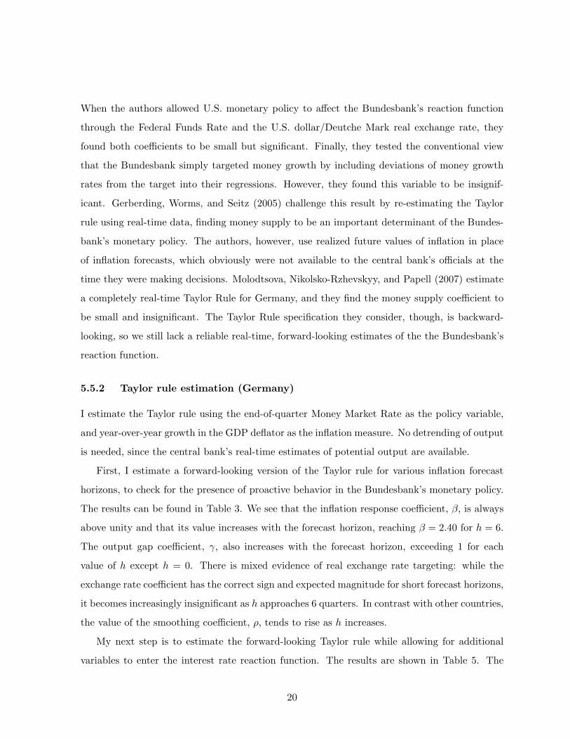
5.5.2 Taylor rule estimation (Germany)

I estimate the Taylor rule using the end-of-quarter Money Market Rate as the policy variable,

and year-over-year growth in the GDP deflator as the inflation measure. No detrending of output

is needed, since the central bank’s real-time estimates of potential output are available.

First, I estimate a forward-looking version of the Taylor rule for various inflation forecast

horizons, to check for the presence of proactive behavior in the Bundesbank’s monetary policy.

The results can be found in Table 3. We see that the inflation response coefficient, β, is always

above unity and that its value increases with the forecast horizon, reaching β = 2.40 for h = 6.

The output gap coefficient, γ, also increases with the forecast horizon, exceeding 1 for each

value of h except h = 0. There is mixed evidence of real exchange rate targeting: while the

exchange rate coefficient has the correct sign and expected magnitude for short forecast horizons,

it becomes increasingly insignificant as h approaches 6 quarters. In contrast with other countries,

the value of the smoothing coefficient, ρ, tends to rise as h increases.

My next step is to estimate the forward-looking Taylor rule while allowing for additional

variables to enter the interest rate reaction function. The results are shown in Table 5. The

20

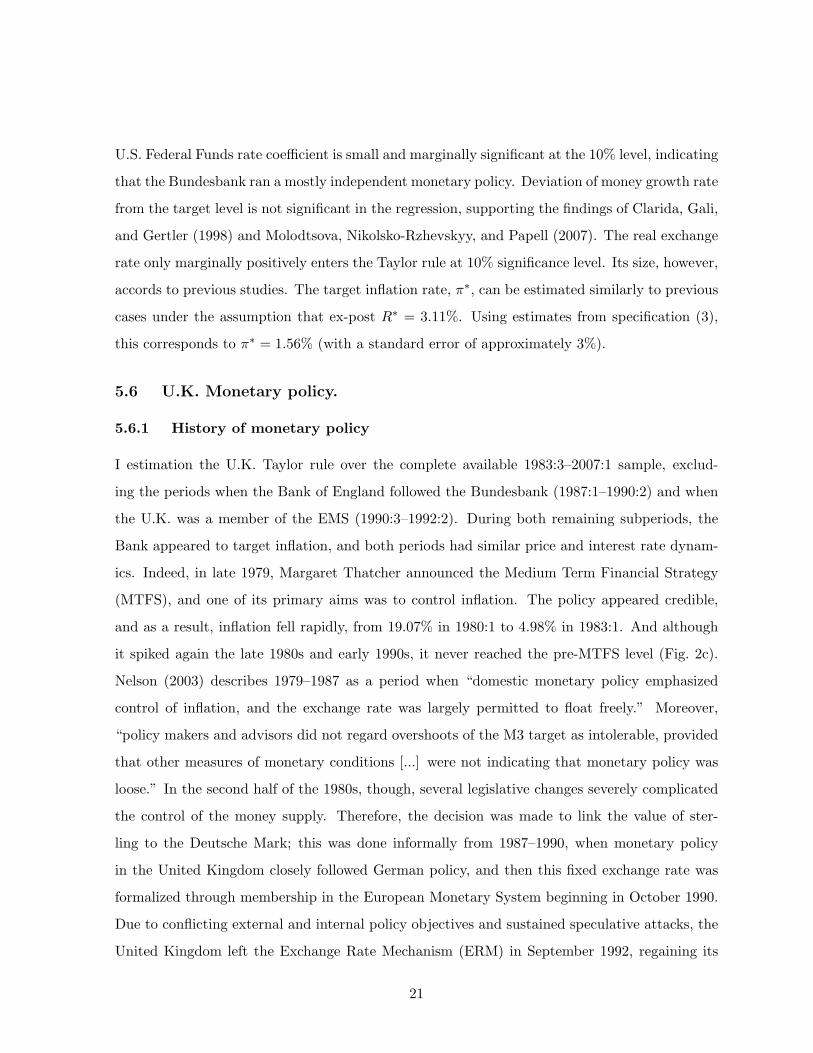
U.S. Federal Funds rate coefficient is small and marginally significant at the 10% level, indicating

that the Bundesbank ran a mostly independent monetary policy. Deviation of money growth rate

from the target level is not significant in the regression, supporting the findings of Clarida, Gali,

and Gertler (1998) and Molodtsova, Nikolsko-Rzhevskyy, and Papell (2007). The real exchange

rate only marginally positively enters the Taylor rule at 10% significance level. Its size, however,

accords to previous studies. The target inflation rate, π∗, can be estimated similarly to previous

cases under the assumption that ex-post R∗ = 3.11%. Using estimates from specification (3),

this corresponds to π∗ = 1.56% (with a standard error of approximately 3%).

5.6 U.K. Monetary policy.

5.6.1 History of monetary policy

I estimation the U.K. Taylor rule over the complete available 1983:3–2007:1 sample, exclud-

ing the periods when the Bank of England followed the Bundesbank (1987:1–1990:2) and when

the U.K. was a member of the EMS (1990:3–1992:2). During both remaining subperiods, the

Bank appeared to target inflation, and both periods had similar price and interest rate dynam-

ics. Indeed, in late 1979, Margaret Thatcher announced the Medium Term Financial Strategy

(MTFS), and one of its primary aims was to control inflation. The policy appeared credible,

and as a result, inflation fell rapidly, from 19.07% in 1980:1 to 4.98% in 1983:1. And although

it spiked again the late 1980s and early 1990s, it never reached the pre-MTFS level (Fig. 2c).

Nelson (2003) describes 1979–1987 as a period when “domestic monetary policy emphasized

control of inflation, and the exchange rate was largely permitted to float freely.” Moreover,

“policy makers and advisors did not regard overshoots of the M3 target as intolerable, provided

that other measures of monetary conditions [...] were not indicating that monetary policy was

loose.” In the second half of the 1980s, though, several legislative changes severely complicated

the control of the money supply. Therefore, the decision was made to link the value of ster-

ling to the Deutsche Mark; this was done informally from 1987–1990, when monetary policy

in the United Kingdom closely followed German policy, and then this fixed exchange rate was

formalized through membership in the European Monetary System beginning in October 1990.

Due to conflicting external and internal policy objectives and sustained speculative attacks, the

United Kingdom left the Exchange Rate Mechanism (ERM) in September 1992, regaining its

21

monetary independence. Clarida, Gali, and Gertler (1998) estimate a simple Taylor Rule regres-

sion over a 1979–1990 sample and find that the Bank of England’s inflation response coefficient

was below unity. When they enhance the Taylor Rule with the Bundesbank’s interest rate,

they find a statistically significant coefficient of 0.60. The authors interpret this result to mean

that the Bank of England followed German monetary policy during this time period, but Nelson

(2003) argues that combining the 1979–1987 and 1987–1990 periods into one sample is imprecise

due to significant differences between U.K. monetary policies during these regimes: While the

Bank of England followed the Bundesbank almost one-for-one during the latter period, it acting

independently during the former period.

The post-1992 period is uniformly agreed to be a period of inflation targeting, with a forward-

looking Taylor-type rule playing an important role in U.K. monetary policy. According to the

1998 Bank of England Act, the bank’s current objectives are to support the government’s eco-

nomic policy with respect to economic growth and unemployment, subject to a price stability

commitment (Davradakis and Taylor (2006)). This policy closely resembles the objectives and

behavior of monetary authorities during 1979–1987. Indeed, both regimes promoted price sta-

bility and successfully restrained inflation, although empirical results for the post-1992 sample

are controversial. Davradakis and Taylor (2006) estimate a non-linear Taylor Rule over the

1992–2003 period, finding that the Bank of England’s monetary policy can be described as con-

sisting of two regimes: a standard stabilizing Taylor Rule model when inflation exceeds 3.1%,

and essentially a RW when inflation is less than or equal to 3.1%. Applying this model to a

quarterly real-time dataset would result in just 15 effective observations, which is not enough

to obtain credible results. Nelson (2003) estimates the backward-looking Taylor rule for 1992–

1997, finding an insignificant coefficient for inflation. The forward-looking specification, though,

results in a stabilizing Taylor Rule with coefficients close to the classical 1.5 and 0.5 for inflation

and the output gap, respectively.

5.6.2 Taylor rule estimation (U.K.)

Following standard practice, I use the tree month Treasury Bill rate as a proxy for the central

bank policy variable, year-over-year growth in the GDP deflator as the inflation measure, and

I define the output gap as deviation from a quadratic time trend over the last 20 years. The

22

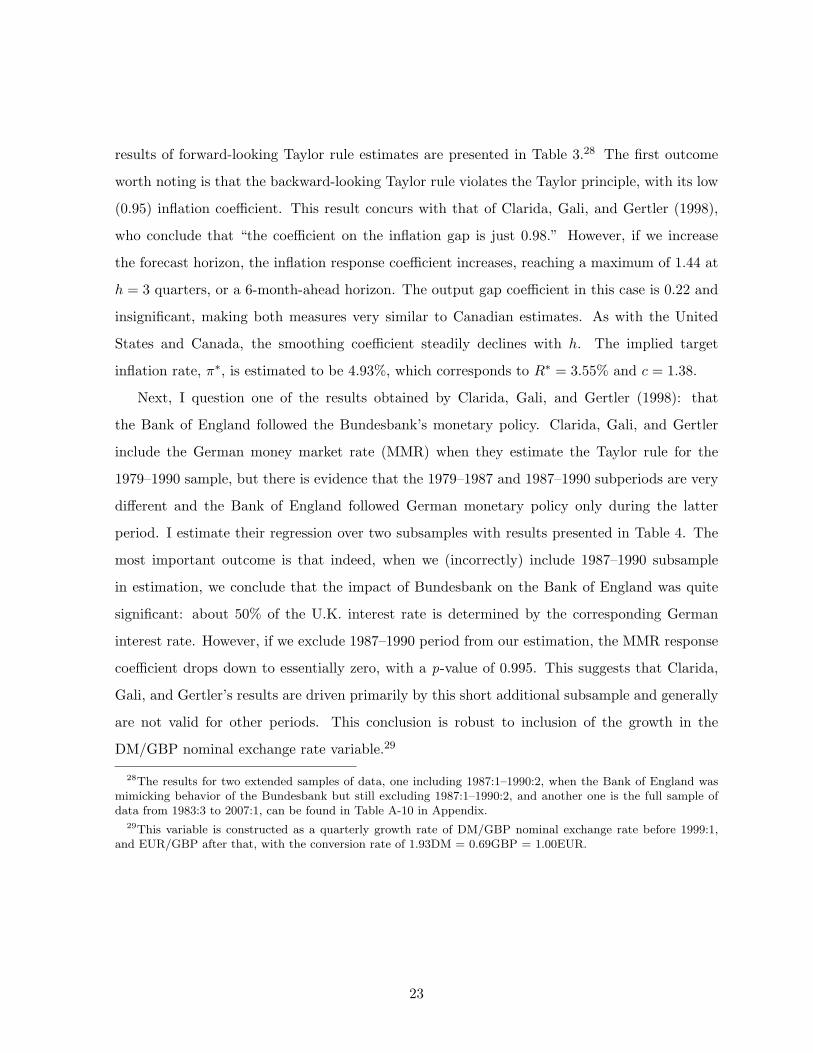
results of forward-looking Taylor rule estimates are presented in Table 3.28 The first outcome

worth noting is that the backward-looking Taylor rule violates the Taylor principle, with its low

(0.95) inflation coefficient. This result concurs with that of Clarida, Gali, and Gertler (1998),

who conclude that “the coefficient on the inflation gap is just 0.98.” However, if we increase

the forecast horizon, the inflation response coefficient increases, reaching a maximum of 1.44 at

h = 3 quarters, or a 6-month-ahead horizon. The output gap coefficient in this case is 0.22 and

insignificant, making both measures very similar to Canadian estimates. As with the United

States and Canada, the smoothing coefficient steadily declines with h. The implied target

inflation rate, π∗, is estimated to be 4.93%, which corresponds to R∗ = 3.55% and c = 1.38.

Next, I question one of the results obtained by Clarida, Gali, and Gertler (1998): that

the Bank of England followed the Bundesbank’s monetary policy. Clarida, Gali, and Gertler

include the German money market rate (MMR) when they estimate the Taylor rule for the

1979–1990 sample, but there is evidence that the 1979–1987 and 1987–1990 subperiods are very

different and the Bank of England followed German monetary policy only during the latter

period. I estimate their regression over two subsamples with results presented in Table 4. The

most important outcome is that indeed, when we (incorrectly) include 1987–1990 subsample

in estimation, we conclude that the impact of Bundesbank on the Bank of England was quite

significant: about 50% of the U.K. interest rate is determined by the corresponding German

interest rate. However, if we exclude 1987–1990 period from our estimation, the MMR response

coefficient drops down to essentially zero, with a p-value of 0.995. This suggests that Clarida,

Gali, and Gertler’s results are driven primarily by this short additional subsample and generally

are not valid for other periods. This conclusion is robust to inclusion of the growth in the

DM/GBP nominal exchange rate variable.29

28The results for two extended samples of data, one including 1987:1–1990:2, when the Bank of England wasmimicking behavior of the Bundesbank but still excluding 1987:1–1990:2, and another one is the full sample ofdata from 1983:3 to 2007:1, can be found in Table A-10 in Appendix.

29This variable is constructed as a quarterly growth rate of DM/GBP nominal exchange rate before 1999:1,and EUR/GBP after that, with the conversion rate of 1.93DM = 0.69GBP = 1.00EUR.

23

6 Conclusions

This paper provides an overview of monetary policies in the United States, Canada, Germany,

and the United Kingdom over the last 25 years through estimation of forward-looking monetary

policy reaction functions when real-time forward-looking data is not available. This issue is

extremely important for countries outside the United States, where central banks do not regularly

release their forecasts to the public; and for the U.S., because forecasts are released with a five-

year lag.

In order to estimate a central bank’s real-time interest rate reaction function, it is crucial

to develop real-time forecasts of the inflation rate and the output gap when this data is not

available. The Greenbook U.S. output gap forecast can be well described by a simple quadratic

detrending, while many other popular detrending methods produce results significantly different

from the Fed’s internal estimates. Greenbook inflation forecasts can be closely replicated using

Bayesian model averaging over various lag lengths of the ADL model in inflation and the GDP

growth rate. Other aggregate methods also typically produce forecasts superior to single model

projections. The paper proceeds to use these forecasts in order to estimate forward-looking

Taylor rules in the absence of forward-looking data. The results show that since the 1980s, the

Fed, the Bank of Canada, the Bundesbank, and the Bank of England have pursued inflation-

targeting monetary policy. However, while the United States and Germany targeted inflation

one-year-ahead, the United Kingdom and Canada focused on the middle-term of roughly two

quarters hence. Despite these differences, all four central banks obeyed the Taylor principle of

having an inflation response coefficient greater than one.

At the present time, the proposed methodology can be applied only to a limited number of

countries, for which relatively long real-time datasets are available. Moreover, the methodology

considers only a limited amount of information, especially at the inflation forecasting stage,

due to a small number of variables recorded. With further development of real-time data, this

research can be expanded beyond the U.S., Canada, the U.K., and Germany as real-time datasets

for other countries get longer, and the methodology can be significantly improved as the existing

datasets become wider.

24

Aiolfi, M. and Timmermann, A. 2006. Persistence in forecasting performance and conditional

combination strategies. Journal of Econometrics, Elsevier, vol. 127(1-2), pages 31-53

Ang, A., Bekaert, G., and Wei M., 2007. Do macro variables, asset markets, or surveys

forecast inflation better? Journal of Monetary Economics, Elsevier, vol. 54(4), pages 1163-

1212, May

Atkeson A. and Ohanian, L., 2001. Are Phillips curves useful for forecasting inflation?

Quarterly Review, Federal Reserve Bank of Minneapolis, issue Win, pages 2-11

Armour J., Fung B., and Maclean, D., 2002. Taylor Rules in the Quarterly Projection Model.

Working Papers 02-1, Bank of Canada

Aruoba B., 2007. Data revisions are not well-behaved. Journal of Money, Credit and Bank-

ing, forthcoming

Bates, J.M. and Granger, C.W.J., 1969. The combination of forecasts. Operations Research

Quarterly, 20, pp. 451-468

Baxter M. and King R., 1999. Measuring Business Cycles: Approximate Band-Pass Filters

For Economic Time Series. The Review of Economics and Statistics, MIT Press, vol. 81(4),

pages 575-593, November

Beffy, P.-O., Ollivaud, P., Richardson, R. and Sedillot, F., 2006. New OECD Methods for

Supply-Side and Medium-Term Assessments: A Capital Services Approach. OECD Economics

Department Working Paper no. 482, July 2006.

Bernanke, B. and Boivin , J., 2003. Monetary policy in a data-rich environment. Journal of

Monetary Economics, 50, pp. 525-546

Beveridge, S. and Nelson, C., 1981. A new approach to decomposition of economic time

series into permanent and transitory components with particular attention to measurement of

the “business cycle”, Journal of Monetary Economics, Elsevier, vol. 7(2), pages 151-174

Branch W. and Evans, G., 2005. A simple recursive forecasting model. Economics Letters,

Elsevier, vol. 91(2), pages 158-166, May

Cayen, J.-P. and van Norden, S., 2005. The reliability of Canadian output-gap estimates.

The North American Journal of Economics and Finance, Elsevier, vol. 16(3), pages 373-393,

December

Clark, P., 1987. The cyclical component of U.S. economic activity. Quarterly journal of

25

Economics 102(4), 1987, pp. 797-814

Clarida, R., Gali, J. and Gertler, M., 1998. Monetary policy rules in practice. Some inter-

national evidence. European Economic Review 42, pp. 1033-1067

Clausen J. and Meier C.-P., 2005. Did the Bundesbank Follow a Taylor Rule? An Analysis

Based on Real-Time Data. Swiss Journal of Economics and Statistics (SJES), Swiss Society of

Economics and Statistics (SSES), vol. 127(II), pages 213-246, June

Cochrane, J., 1994. Permanent and transitory components of GNP and stock prices. Quar-

terly Journal of Economics, vol. 109 (February) pp. 241-265

Corradi, Valentina, Andres Fernandez and Norman R. Swanson, 2007. Information in the

Revision Process of Real-Time Data. Working paper

Cote, D., Lam J-P., Liu Y. and St-Amant, P. 2002. The Role of Simple Rules in the Conduct

of Canadian Monetary Policy. Bank of Canada Review, Bank of Canada, vol. 127(Spring), pages

27-35

Croushore, D., 2007. An evaluation of inflation forecasts from surveys using real-time data.

Working Papers 06-19, Federal Reserve Bank of Philadelphia

Croushore, D. and Stark, T., 2001. A Real-Time Data Set for Macroeconomists. Journal of

Econometrics, 2001, 105, 111-130

Curtis, D., 2005. Monetary Policy and Economic Activity in Canada in the 1990s. Canadian

Public Policy, University of Toronto Press, vol. 31(1), pages 59-78, March

Davradakis, E. and Taylor, M., 2006. Interest rate setting and inflation targeting: evi-

dence of a nonlinear Taylor rule for the United Kingdom. Studies in Nonlinear Dynamics and

Econometrics, Volume 10, issue 4

Edge, R., Kiley, M. and Laforte, J.-P., 2007. Natural rate measures in an estimated ESGE

model of the U.S. economy. Finance and Economics Discussion Series 2007-8, Washington:

Board of Governors of the Federal Reserve System, March

Egginton, D., Pick, A., and Vahey, S., 2002. ’Keep it real!’: a real-time UK macro data set.

Economics Letters, Elsevier, vol. 77(1), pages 15-20, September

Faust, J., Rogers, J., and Wright, J., 2003. Exchange rate forecasting: the errors we’ve really

made. Journal of International Economics, Elsevier, vol. 60(1), pages 35-59, May

Faust, J., Rogers, J., and Wright, J., 2005. News and noise in G7 GDP announcements.

26

Journal of Money, Credit and Banking, Blackwell Publishing, vol. 37(3), pages 403-19, June

Faust, J. and Wright, J., 2007. Comparing Greenbook and reduced form forecasts using

large realtime dataset. NBER Working Papers 13397, National Bureau of Economic Research,

Inc.

Fernandez, A. and Nikolsko-Rzhevskyy, A., 2007. Measuring the Taylor Rule’s Performance.

Economic Letter–Insights from the Federal Reserve Bank of Dallas, Vol. 2, No. 6 June 2007

Fortin, P., 1996. The Great Canadian Slump. Canadian Journal of Economics, Canadian

Economics Association, vol. 29(4), pages 761-87, November

Garratt, A., Koop, G., and Vahey, S., 2006. Forecasting Substantial Data Revisions in

the Presence of Model Uncertainty. Birkbeck Working Papers in Economics and Finance 0617,

Birkbeck, School of Economics, Mathematics and Statistics.

Garratt, A., Koop, G., Mise, E. and Vahey, S., 2007. Real-time prediction with UK monetary

aggregates in the presence of model uncertainty. Birkbeck Working Papers in Economics and

Finance 0714, Birkbeck, School of Economics, Mathematics and Statistics

Gerberding, C., Worms, A. and Seitz, F., 2005. How the Bundesbank really conducted

monetary policy. The North American Journal of Economics and Finance Volume 16, Issue 3,

December 2005, Pages 277-292

Hodrick, R. J., and Prescott, E. C., 1997. Postwar U.S. Business Cycles: An Empirical

Investigation. Journal of Money, Credit and Banking 29 (1), Feb. 1997, 1-16

Koenig, E., 2004. Monetary policy prospects. Economic and Financial Policy Review,

Federal Reserve Bank of Dallas, pages 1-16

Koenig, E., Dolmas, S., and Piger, J., 2003. The Use and Abuse of Real-Time Data in

Economic Forecasting. The Review of Economics and Statistics, MIT Press, vol. 85(3), pages

618-628, 07.

Kuttner, K.. 1994. Estimating potential output as a latent variable. Journal of Business

and Economic Statistics, vol. 12 (July) pp. 361-368

Kydland, F. and Prescott, E. 1992. Time to build and aggregate fluctuations. Econometrica,

vol. 50 (November) pp. 361-368

Lansing, K., 2002. Real-time estimation of trend output and the illusion of interest rate

smoothing. Economic Review, Federal Reserve Bank of San Francisco, pages 17-34

27

Mankiw, G. and Shapiro, M., 1986. News or Noise? Analysis of GNP Revisions. Survey of

Current Business, Vol. 66, pp. 20-25, May 1986

Marcellino, M., Stock, J. and Watson, M., 2006. A comparison of direct and iterated multi-

step AR methods for forecasting macroeconomic time series. Journal of Econometrics, Elsevier,

vol. 127(1-2), pages 499-526

Mishkin, F., 2007. Estimating potential output. Remarks by Governor Federic S. Mishkin

at the Conference on Price Measurement for Monetary Policy, Federal Reserve Bank of Dallas,

Dallas, TX, May 24

Molodtsova, T., Nikolsko-Rzhevskyy, A. and Papell, D., 2007. Taylor Rules and Real-Time

Data: A Tale of Two Countries and One Exchange Rate. Working paper

Morley, J., Nelson C. and Zivot, E. 2003. Why are Beveridge-Nelson and Unobserved-

component decompositions of GDP so Different? Review of Economics and Statistics, vol. 85

(May 2003), 235-243

Murray, C., Nikolsko-Rzhevskyy, A. and Papell, D., 2007. Inflation Persistence and the

Taylor Principle. Working paper

Neiss K. and Nelson, E. 2005. Inflation dynamics, marginal cost, and the output gap:

evidence from three countries. Journal of Money, Credit and Banking, vol. 37 (December) pp.

1019-1045

Nelson, E. 2003. UK monetary policy 1972–97: a guide using Taylor rules. Central Banking,

Monetary Theory and Practice: Essays in Honour of Charles Goodhart, Volume One. Chel-

tenham, UK: Edward Elgar, 2003, pp. 195-216

Nocetti, D., and Smith, W., 2006. Why do pooled forecasts do better than individual

forecasts ex post? Economics Bulletin, Vol. 4, No. 36 pp. 1-7

Okun, A., 1962, Potential GNP: Its Measurement and Significance. Proceedings of the Busi-

ness and Economic Statistics Section, American Statistical Association, Washington, D.C., pp.

98-103

Orphanides, A., 2001. Monetary Policy Rules Based on Real-Time Data. American Eco-

nomic Review, American Economic Association, vol. 91(4), pages 964-985, September

Orphanides, A., 2003. Historical monetary policy analysis and the Taylor rule. Journal of

Monetary Economics, Elsevier, vol. 50(5), pages 983-1022, July

28

Orphanides, A., 2004. Monetary Policy Rules, Macroeconomic Stability, and Inflation: A

View from the Trenches. Journal of Money, Credit and Banking, Blackwell Publishing, vol.

36(2), pages 151-75, April

Orphanides, A. and van Norden, S., 2005. The reliability of inflation forecasts based on

output gap estimates in real time. Journal of Money, Credit, and Banking - Volume 37, Number

3, June 2005, pp. 583-601

Rapach D. and Strauss, J. 2007. Forecasting real housing price growth in eight district states.

Federal Reserve Bank of St. Louis Regional Economic Development, forthcoming

Romer C. and Romer, D. 2000. Federal Reserve Information and the Behavior of Interest

Rates. American Economic Review, American Economic Association, vol. 90(3), pages 429-457,

June

Rudebusch, G., 2006. Monetary Policy Inertia: Fact or Fiction? International Journal of

Central Banking, International Journal of Central Banking, vol. 2(4), December

Staiger, D., Stock, J. and Watson, M., 1997. The NAIRU, unemployment, and monetary

policy. Journal of Economic Perspectives, vol. 11 (Winter) pp. 33-49

Svensson, L., 1999. Inflation targeting: some extensions. Scandinavian Journal of Eco-

nomics, Blackwell Publishing, vol. 101(3), pages 337-61, September

Taylor, J., 1993. Discretion versus policy rules in practice. Carnegie-Rochester Conference

on Public Policy 39, pp. 195-214

Thiessen, G., 2000. Can a bank change? The evolution of monetary policy at the Bank

of Canada 1935-2000. Lecture by Gordon Thiessen, Governor of the Bank of Canada, to the

Faculty of Social Science University of Western Ontario, London, Ontario, 17 October 2000

van Norden, S., 1995. Why is it so hard to measure the current output gap? Macroeconomics

9506001, EconWPA

Wallis, K., 1999. Asymmetric density forecasts of inflation and the Bank of Englands fan

chart. National Institute Economic Review, 106112

Watson M., 2007. How accurate are real-time estimates of output trends and gaps? Economic

Quarterly, Federal Reserve Bank of Richmond, issue Spr, pages 143-161

Wynne M. and Solomon, G., 2007. Obstacles to measuring global output gaps. Federal

Reserve Bank of Dallas, Economic Letter, Vol. 2, No. 3, March 2007

29

Table 1: The relative performance of various detrending methods in reproducing Greenbook1-quarter-back output gap estimates during 1969:1–1997:4

Model RMSPE Sign Test Correlation

1. Quadratic 3.651 4.45 0.872. Linear 4.473 5.19 0.303. Rolling window (Quadratic)

Window = 40 4.645 2.23 0.56Window = 80 3.320 4.64 0.85Window = 120 2.837 5.57 0.77Window = 160 3.759 5.20 0.48

4. Constant gain (Quadratic)Gain = 0.005 3.564 5.20 0.88Gain = 0.010 3.557 5.01 0.87Gain = 0.015 3.672 5.01 0.84Gain = 0.020 3.947 4.46 0.80

5. Hodrick-Prescott λ=1600Original 5.438 0.19 0.29Extended by K=12 4.789 2.97 0.56

6. Band pass filterExtended by K=12 4.841 2.78 0.54Extended by K=100 5.084 0.00 0.45

7. Unobserved Component 3.668 5.75 0.608. Beveridge-Nelson 5.811 -1.11 -0.06

Notes: All models are estimated over the latest real-time vintage of data (“current vintage”). The window size isexpressed in quarters. “Constant gain” discounts past observations geometrically. “Hodrick-Prescott extended”forecasts the (log of) real GDP by K periods into both directions before applying the filter; refer to Baxter andKing (1999) for details. “Band pass” filters frequencies between 6 and 32 quarters. The number of MA termsin the filter equals the number of forecasted periods K. The choice of K and the forecasting model accordsto Watson (2007). The “Unobserved Component” model corresponds to Clark (1987). The “Beveridge-Nelson”decomposition follows Beveridge and Nelson (1981). The Greenbook output gap data comes from Orphanides(2003). RMSPE stands for “Root Mean Square Prediction Error.” The Sign Test is the direction of change testwith the null of no predictability.

30

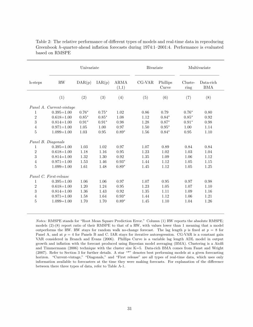
Table 2: The relative performance of different types of models and real-time data in reproducingGreenbook h-quarter-ahead inflation forecasts during 1974:1–2001:4. Performance is evaluatedbased on RMSPE

Univariate Bivariate Multivariate

h-steps RW DAR(p) IAR(p) ARMA CG-VAR Phillips Cluste- Data-rich(1,1) Curve ring BMA

(1) (2) (3) (4) (5) (6) (7) (8)

Panel A. Current-vintage1 0.395=1.00 0.76∗ 0.75∗ 1.02 0.86 0.79 0.76∗ 0.802 0.618=1.00 0.85∗ 0.85∗ 1.08 1.12 0.84∗ 0.85∗ 0.923 0.814=1.00 0.91∗ 0.91∗ 0.98 1.28 0.87∗ 0.91∗ 0.984 0.971=1.00 1.05 1.00 0.97 1.50 0.95∗ 1.00 1.145 1.099=1.00 1.03 0.95 0.89∗ 1.56 0.84∗ 0.95 1.10

Panel B. Diagonals1 0.395=1.00 1.03 1.02 0.97 1.07 0.89 0.84 0.842 0.618=1.00 1.18 1.16 0.95 1.23 1.02 1.03 1.043 0.814=1.00 1.32 1.30 0.92 1.35 1.09 1.06 1.124 0.971=1.00 1.53 1.46 0.93∗ 1.44 1.12 1.05 1.155 1.099=1.00 1.61 1.48 0.89∗ 1.45 1.12 1.05 1.25

Panel C. First-release1 0.395=1.00 1.06 1.06 0.97 1.07 0.95 0.97 0.982 0.618=1.00 1.20 1.24 0.95 1.23 1.05 1.07 1.103 0.814=1.00 1.36 1.43 0.92 1.35 1.11 1.09 1.164 0.971=1.00 1.58 1.64 0.93∗ 1.44 1.12 1.06 1.215 1.099=1.00 1.70 1.70 0.89∗ 1.45 1.10 1.04 1.26

Notes: RMSPE stands for “Root Mean Square Prediction Error.” Column (1) RW reports the absolute RMSPE;models (2)-(8) report ratio of their RMSPE to that of a RW, with values lower than 1 meaning that a modeloutperforms the RW. RW stays for random walk no-change forecast. The lag length p is fixed at p = 8 forPanel A, and at p = 4 for Panels B and C. IAR stays for iterative autoregression. CG-VAR is a constant gainVAR considered in Branch and Evans (2006). Phillips Curve is a variable lag length ADL model in outputgrowth and inflation with the forecast produced using Bayesian model averaging (BMA). Clustering is a Aiolfiand Timmermann (2006) technique with the cluster size K=5. Data-rich BMA comes from Faust and Wright(2007). Refer to Section 3 for further details. A star “*” denotes best performing models at a given forecastinghorizon. “Current-vintage,” “Diagonals,” and “First release” are all types of real-time data, which uses onlyinformation available to forecasters at the time they were making forecasts. For explanation of the differencebetween there three types of data, refer to Table A-1.

31

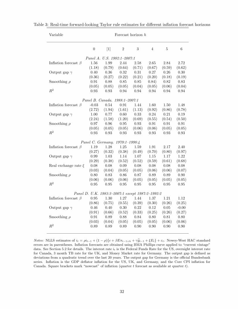
Table 3: Real-time forward-looking Taylor rule estimates for different inflation forecast horizons

Variable Forecast horizon h

0 [1] 2 3 4 5 6

Panel A. U.S. 1982:1–2007:1Inflation forecast β 1.56 1.99 2.44 2.58 2.65 2.84 2.72

(1.18) (0.79) (0.64) (0.71) (0.67) (0.59) (0.62)Output gap γ 0.40 0.36 0.32 0.31 0.27 0.26 0.30

(0.36) (0.27) (0.22) (0.21) (0.20) (0.18) (0.19)Smoothing ρ 0.91 0.88 0.85 0.85 0.84) 0.82 0.83

(0.05) (0.05) (0.05) (0.04) (0.05) (0.06) (0.04)R2 0.93 0.93 0.94 0.94 0.94 0.94 0.94

Panel B. Canada. 1988:1–2007:1Inflation forecast β -0.03 0.54 0.91 1.44 1.60 1.50 1.48

(2.72) (1.94) (1.61) (1.13) (0.92) (0.86) (0.78)Output gap γ 1.00 0.77 0.60 0.33 0.24 0.21 0.19

(2.24) (1.58) (1.20) (0.69) (0.55) (0.54) (0.50)Smoothing ρ 0.97 0.96 0.95 0.93 0.91 0.91 0.91

(0.05) (0.05) (0.05) (0.06) (0.06) (0.05) (0.05)R2 0.93 0.93 0.93 0.93 0.93 0.93 0.93

Panel C. Germany. 1979:1–1998:4Inflation forecast β 1.19 1.28 1.25 1.59 1.91 2.17 2.40

(0.27) (0.32) (0.38) (0.49) (0.70) (0.80) (0.97)Output gap γ 0.99 1.03 1.14 1.07 1.15 1.17 1.22

(0.29) (0.38) (0.52) (0.52) (0.59) (0.61) (0.68)Real exchange rate ξ 0.08 0.08 0.09 0.08 0.08 0.08 0.08

(0.03) (0.04) (0.05) (0.05) (0.06) (0.06) (0.07)Smoothing ρ 0.80 0.83 0.86 0.87 0.89 0.89 0.90

(0.06) (0.06) (0.06) (0.05) (0.05) (0.05) (0.05)R2 0.95 0.95 0.95 0.95 0.95 0.95 0.95

Panel D. U.K. 1983:3–2007:1 except 1987:2–1992:2Inflation forecast β 0.95 1.30 1.27 1.44 1.37 1.21 1.12

(0.86) (0.75) (0.55) (0.39) (0.30) (0.26) (0.25)Output gap γ 0.46 0.40 0.30 0.22 0.12 0.05 -0.00

(0.91) (0.66) (0.52) (0.33) (0.25) (0.26) (0.27)Smoothing ρ 0.91 0.89 0.88 0.84 0.80 0.81 0.80

(0.03) (0.04) (0.05) (0.05) (0.05) (0.06) (0.06)R2 0.89 0.89 0.89 0.90 0.90 0.90 0.90

Notes: NLLS estimates of it = ρit−1 + (1 − ρ)c + βEπt−1+h + γyt−1 + ξEt + εt. Newey-West HAC standarderrors are in parentheses. Inflation forecasts are obtained using BMA Phillips curve applied to “current vintage”data. See Section 5.2 for details. The interest rate it is the Federal Funds Rate for the US, overnight interest ratefor Canada, 3 month TB rate for the UK, and Money Market rate for Germany. The output gap is defined asdeviations from a quadratic trend over the last 20 years. The output gap for Germany is the official Bundesbankseries. Inflation is the GDP deflator inflation for the US, UK, and Germany, and the Core CPI inflation forCanada. Square brackets mark “nowcast” of inflation (quarter t forecast as available at quarter t).

32

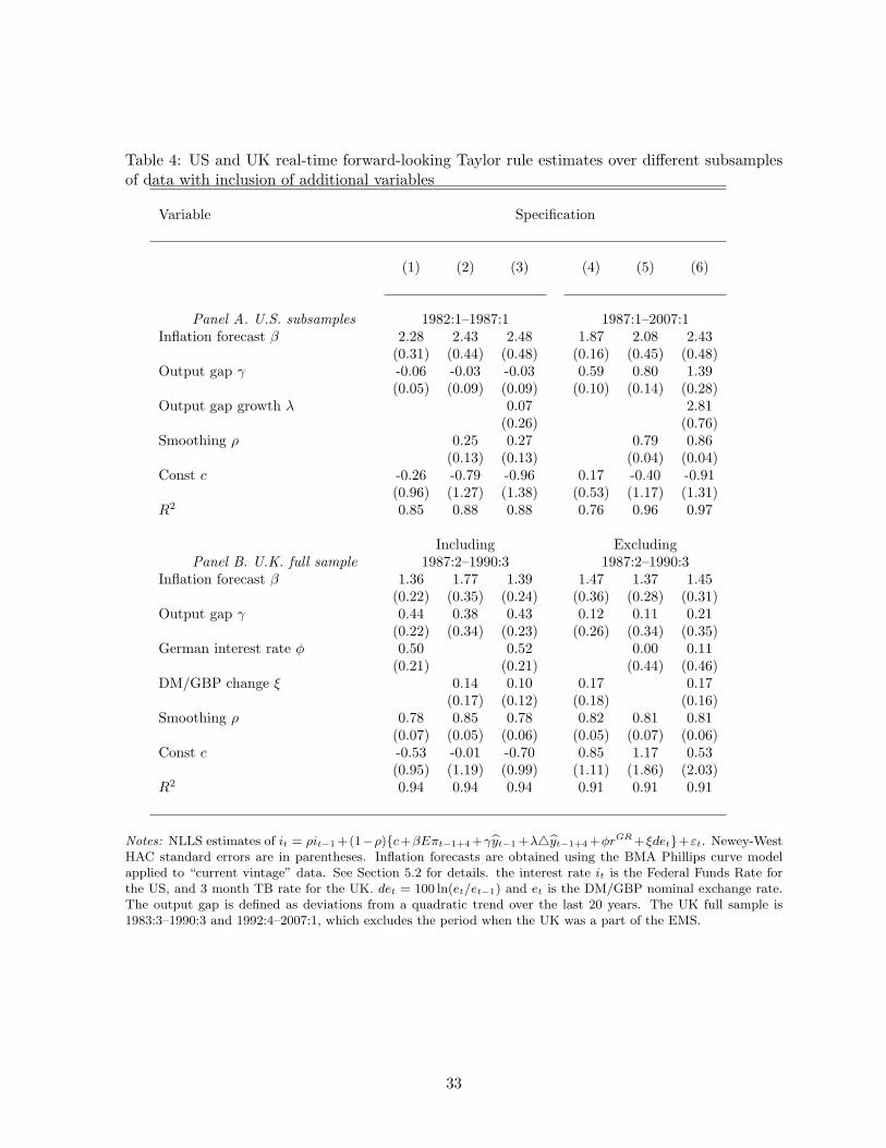
Table 4: US and UK real-time forward-looking Taylor rule estimates over different subsamplesof data with inclusion of additional variables

Variable Specification

(1) (2) (3) (4) (5) (6)

Panel A. U.S. subsamples 1982:1–1987:1 1987:1–2007:1Inflation forecast β 2.28 2.43 2.48 1.87 2.08 2.43

(0.31) (0.44) (0.48) (0.16) (0.45) (0.48)Output gap γ -0.06 -0.03 -0.03 0.59 0.80 1.39

(0.05) (0.09) (0.09) (0.10) (0.14) (0.28)Output gap growth λ 0.07 2.81

(0.26) (0.76)Smoothing ρ 0.25 0.27 0.79 0.86

(0.13) (0.13) (0.04) (0.04)Const c -0.26 -0.79 -0.96 0.17 -0.40 -0.91

(0.96) (1.27) (1.38) (0.53) (1.17) (1.31)R2 0.85 0.88 0.88 0.76 0.96 0.97

Including ExcludingPanel B. U.K. full sample 1987:2–1990:3 1987:2–1990:3

Inflation forecast β 1.36 1.77 1.39 1.47 1.37 1.45(0.22) (0.35) (0.24) (0.36) (0.28) (0.31)

Output gap γ 0.44 0.38 0.43 0.12 0.11 0.21(0.22) (0.34) (0.23) (0.26) (0.34) (0.35)

German interest rate φ 0.50 0.52 0.00 0.11(0.21) (0.21) (0.44) (0.46)

DM/GBP change ξ 0.14 0.10 0.17 0.17(0.17) (0.12) (0.18) (0.16)

Smoothing ρ 0.78 0.85 0.78 0.82 0.81 0.81(0.07) (0.05) (0.06) (0.05) (0.07) (0.06)

Const c -0.53 -0.01 -0.70 0.85 1.17 0.53(0.95) (1.19) (0.99) (1.11) (1.86) (2.03)

R2 0.94 0.94 0.94 0.91 0.91 0.91

Notes: NLLS estimates of it = ρit−1 +(1−ρ)c+βEπt−1+4 +γyt−1 +λ4yt−1+4 +φrGR+ξdet+εt. Newey-WestHAC standard errors are in parentheses. Inflation forecasts are obtained using the BMA Phillips curve modelapplied to “current vintage” data. See Section 5.2 for details. the interest rate it is the Federal Funds Rate forthe US, and 3 month TB rate for the UK. det = 100 ln(et/et−1) and et is the DM/GBP nominal exchange rate.The output gap is defined as deviations from a quadratic trend over the last 20 years. The UK full sample is1983:3–1990:3 and 1992:4–2007:1, which excludes the period when the UK was a part of the EMS.

33

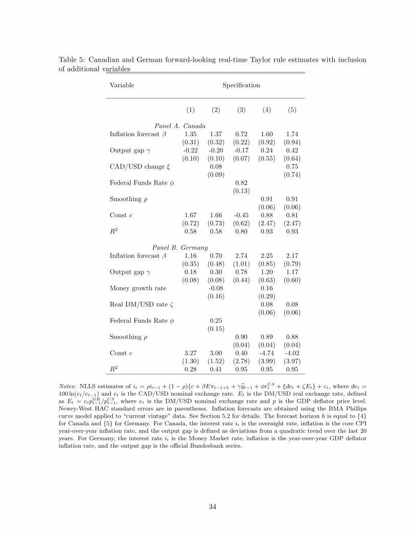
Table 5: Canadian and German forward-looking real-time Taylor rule estimates with inclusionof additional variables

Variable Specification

(1) (2) (3) (4) (5)

Panel A. CanadaInflation forecast β 1.35 1.37 0.72 1.60 1.74

(0.31) (0.32) (0.22) (0.92) (0.94)Output gap γ -0.22 -0.20 -0.17 0.24 0.42

(0.10) (0.10) (0.07) (0.55) (0.64)CAD/USD change ξ 0.08 0.75

(0.09) (0.74)Federal Funds Rate φ 0.82

(0.13)Smoothing ρ 0.91 0.91

(0.06) (0.06)Const c 1.67 1.66 -0.45 0.88 0.81

(0.72) (0.73) (0.62) (2.47) (2.47)R2 0.58 0.58 0.80 0.93 0.93

Panel B. GermanyInflation forecast β 1.16 0.70 2.74 2.25 2.17

(0.35) (0.48) (1.01) (0.85) (0.79)Output gap γ 0.18 0.30 0.78 1.20 1.17

(0.08) (0.08) (0.44) (0.63) (0.60)Money growth rate -0.08 0.16

(0.16) (0.29)Real DM/USD rate ζ 0.08 0.08

(0.06) (0.06)Federal Funds Rate φ 0.25

(0.15)Smoothing ρ 0.90 0.89 0.88

(0.04) (0.04) (0.04)Const c 3.27 3.00 0.40 -4.74 -4.02

(1.30) (1.52) (2.78) (3.99) (3.97)R2 0.28 0.41 0.95 0.95 0.95

Notes: NLLS estimates of it = ρit−1 + (1 − ρ)c + βEπt−1+h + γyt−1 + φrUSt + ξdet + ζEt + εt, where det =100 ln(et/et−1) and et is the CAD/USD nominal exchange rate. Et is the DM/USD real exchange rate, definedas Et = etp

GRt−1/p

USt−1, where et is the DM/USD nominal exchange rate and p is the GDP deflator price level.

Newey-West HAC standard errors are in parentheses. Inflation forecasts are obtained using the BMA Phillipscurve model applied to “current vintage” data. See Section 5.2 for details. The forecast horizon h is equal to 4for Canada and 5 for Germany. For Canada, the interest rate it is the overnight rate, inflation is the core CPIyear-over-year inflation rate, and the output gap is defined as deviations from a quadratic trend over the last 20years. For Germany, the interest rate it is the Money Market rate, inflation is the year-over-year GDP deflatorinflation rate, and the output gap is the official Bundesbank series.

34

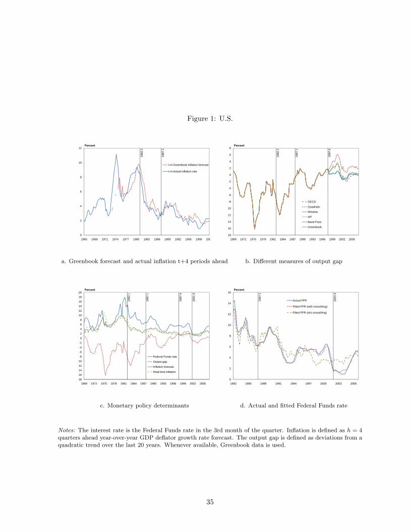
Figure 1: U.S.

8

10

123HUFHQW

t+4 Greenbook inflation forecast

t+4 Actual inflation rate

1982

:1

1987

:1

0

2

4

6

1965 1968 1971 1974 1977 1980 1983 1986 1989 1992 1995 1998 2001

-4

-2

0

2

4

6

83HUFHQW

1982

:1

1987

:1

1997

:4

-18

-16

-14

-12

-10

-8

-6

-4

1969 1972 1975 1978 1981 1984 1987 1990 1993 1996 1999 2002 2005

OECD

Quadratic

Window

HP

Band Pass

Greenbook

a. Greenbook forecast and actual inflation t+4 periods ahead b. Different measures of output gap

2

4

6

8

10

12

14

16

18

203HUFHQW

1982

:1

1987

:1

1997

:4

2001

:4

-18

-16

-14

-12

-10

-8

-6

-4

-2

0

2

1969 1972 1975 1978 1981 1984 1987 1990 1993 1996 1999 2002 2005

Federal Funds rate

Output gap

Inflation forecast

Real-time inflation

3HUFHQW

14

163HUFHQW

Actual FFR1987

:1

2001

:4

12

14Fitted FFR (with smoothing)

Fitted FFR (w/o smoothing)

10

6

8

4

6

2

0

1982 1985 1988 1991 1994 1997 2000 2003 2006

c. Monetary policy determinants d. Actual and fitted Federal Funds rate

Notes: The interest rate is the Federal Funds rate in the 3rd month of the quarter. Inflation is defined as h = 4quarters ahead year-over-year GDP deflator growth rate forecast. The output gap is defined as deviations from aquadratic trend over the last 20 years. Whenever available, Greenbook data is used.

35

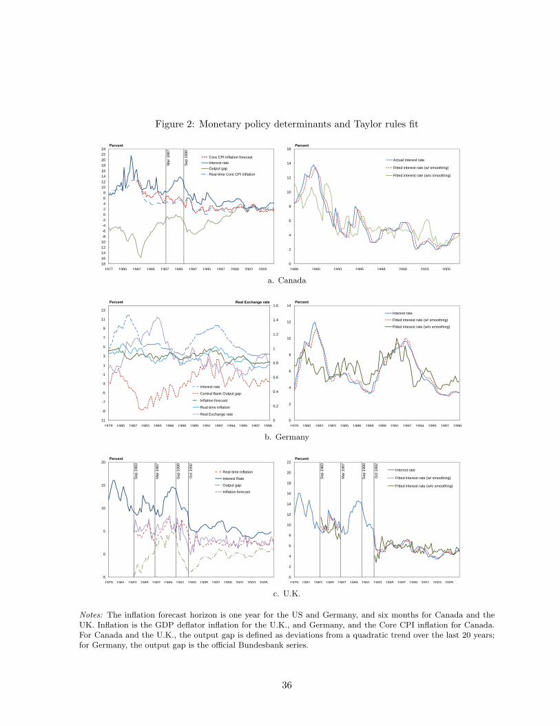
Figure 2: Monetary policy determinants and Taylor rules fit

6

8

10

12

14

16

18

20

22

243HUFHQW

Core CPI inflation forecast

Interest rate

Output gap

Real-time Core CPI inflation

Mar

198

7

Sep

199

0

-18

-16

-14

-12

-10

-8

-6

-4

-2

0

2

4

1977 1980 1982 1985 1987 1990 1992 1995 1997 2000 2002 2005

10

12

14

163HUFHQW

Actual Interest rate

Fitted interest rate (w/ smoothing)

Fitted interest rate (w/o smoothing)

0

2

4

6

8

1988 1990 1993 1995 1998 2000 2003 2005

a. Canada

1

1.2

1.4

1.6

3

5

7

9

11

13

5HDO([FKDQJHUDWH3HUFHQW

0

0.2

0.4

0.6

0.8

-11

-9

-7

-5

-3

-1

1

1979 1980 1982 1983 1985 1986 1988 1989 1991 1992 1994 1995 1997 1998

Interest rate

Central Bank Output gap

Inflation forecast

Real-time inflation

Real Exchange rate

3HUFHQW

12

143HUFHQW

Interest rate

Fitted interest rate (w/ smoothing)

10

12 Fitted interest rate (w/ smoothing)

Fitted interest rate (w/o smoothing)

8

6

4

2

0

1979 1980 1982 1983 1985 1986 1988 1989 1991 1992 1994 1995 1997 1998

b. Germany

10

15

203HUFHQW

Real-time Inflation

Interest Rate

Output gap

Inflation forecast

Sep

198

3

Oct

199

2

Mar

198

7

Sep

199

0

-5

0

5

1979 1981 1983 1985 1987 1989 1991 1993 1995 1997 1999 2001 2003 2005

12

14

16

18

20

223HUFHQW

Interest rate

Fitted interest rate (w/ smoothing)

Fitted interest rate (w/o smoothing)

Sep

198

3

Oct

199

2

Mar

198

7

Sep

199

0

0

2

4

6

8

10

12

1979 1981 1983 1985 1987 1989 1991 1993 1995 1997 1999 2001 2003 2005

c. U.K.

Notes: The inflation forecast horizon is one year for the US and Germany, and six months for Canada and theUK. Inflation is the GDP deflator inflation for the U.K., and Germany, and the Core CPI inflation for Canada.For Canada and the U.K., the output gap is defined as deviations from a quadratic trend over the last 20 years;for Germany, the output gap is the official Bundesbank series.

36

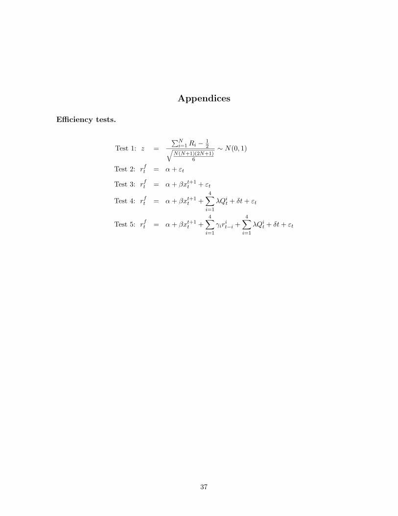
Appendices

Efficiency tests.

Test 1: z =∑Ni=1Ri − 1

2√N(N+1)(2N+1)

6

∼ N(0, 1)

Test 2: rft = α+ εt

Test 3: rft = α+ βxt+1t + εt

Test 4: rft = α+ βxt+1t +

4∑i=1

λQit + δt+ εt

Test 5: rft = α+ βxt+1t +

4∑i=1

γirit−i +

4∑i=1

λQit + δt+ εt

37

Table A-1: “Current vintage,” “Diagonals,” and “First release” specifications of real-time databy the example of the U.S. annualized quarterly GDP deflator inflation rate as of the fourthquarter of 1999 (1999:Q4).

Calendar Date Vintage (release) dates

. . . . . . 1998:Q3 1998:Q4 1999:Q1 1999:Q2 1999:Q3 1999:Q4 2000:Q1...

......

......

......

... –1994:03 . . . 2.56 2.56 2.56 2.56 2.56 2.334 –1994:04 . . . 2.65 2.65 2.65 2.65 2.65 1.844 –1995:01 . . . 2.49 2.49 2.49 2.49 2.49 2.894 –1995:02 . . . 1.83 1.83 1.83 1.83 1.83 1.634 –1995:03 . . . 1.90 1.90 1.90 1.90 1.90 1.754 –1995:04 . . . 2.02 2.02 2.02 2.02 2.02 1.904 –1996:01 . . . 2.28 2.28 2.28 2.28 2.28 2.444 –1996:02 . . . 1.20 1.20 1.20 1.20 1.20 1.274 –1996:03 . . . 1.81 1.81 1.81 1.81 1.81 1.714 –1996:04 . . . 1.78 1.78 1.78 1.78 1.78 1.414 –1997:01 . . . 2.80 2.80 2.80 2.80 2.80 2.374 –1997:02 . . . 1.54 1.54 1.54 1.54 1.54 1.514 –1997:03 . . . 1.18♦ 1.18 1.18 1.18 1.18 1.144 –1997:04 . . . 1.17♦ 1.17♦ 1.17 1.17 1.17 1.184 –1998:01 . . . 0.84♦ 0.84♦ 0.84♦ 0.84 0.84 0.904 –1998:02 – 0.85♦? 0.87♦ 0.87♦ 0.87♦ 0.87 1.274 –1998:03 – – 0.82♦? 0.98♦ 0.98♦ 0.98♦ 1.524 –1998:04 – – – 0.83♦? 0.82♦ 0.82♦ 1.024♦ –1999:01 – – – – 1.40♦? 1.59♦ 1.934♦ –1999:02 – – – – – 1.56♦? 1.374♦ –1999:03 – – – – – – 0.944♦? –1999:04 – – – – – – – –

Notes: 4s mark “current vintage” data, ♦s mark “diagonals” data, and ?s mark “first releases” data. “Diagonals”data is shown for the case when 4 lags of unemployment rate are used. Three dots represent data which is(generally) available in 1999:Q4, but is not displayed in this table. “–” means that the data is not available in1999:Q4.

38

Table A-2: Efficiency test results with actuals defined as 2007:Q2 vintage

Wilcoxon Ranking Zero mean Mincer– Quarterly dummies PastTest t-test Zarnowitz and Time trend revisions

(1) (2) (3) (4) (5)

Panel A. Country: USGDP Growth 4.55 2.93 51.07 62.78 64.92GDP Inflation 1.56 1.11 13.25 24.95 30.62CPI Inflation 0.63 0.24 0.07 7.44 9.24Unemployment 2.53 1.63 4.00 7.58 17.01

Panel D. Country: CanadaGDP Growth 4.35 2.88 29.66 28.64 31.47GDP Inflation 2.22 0.7 14.02 23.17 23.88CPI Inflation -0.15 -0.27 0.13 0.31 1.82Unemployment 0.55 -1.21 3.32 8.86 12.72Core CPI Inflation 6.28 1.14 2.22 7.43 7.68

Panel B. Country: GermanyGDP Growth 2.57 1.88 21.85 19.48 24.05GDP Inflation 0.42 -0.15 17.92 17.81 19.62CPI Inflation -0.84 -2.08 4.87 9.64 20.86Money Growth -1.62 -2.76 13.88 34.51 45.09

Panel C. Country: UKGDP Growth 4.69 4.96 53.52 53.86 59.63GDP Inflation 2.69 1.74 69.01 92.84 93.36

Notes: The series being tested is “Revisions” defined as “Actuals–Real-time.” Regression-based tests (2)–(5)employ robust Newey-West standard errors. Test statistics for (3)–(5) come from LR-tests for joint insignificanceof coefficients (including the constant term). (3) assumes the base specification (2) and adds the series of first-releases. (4) assumes (3) plus quarterly dummies and a linear time trend. (5) assumes (4) and adds 4 lags of pastrevisions (Eq. ??). 5% critical values for (1)-(5) are 1.96, 1.96, 5.99, 12.6 and 18.3, respectively.

39

Table A-3: The relative performance of different types of models and real-time data in repro-ducing Greenbook h-quarter-ahead inflation forecasts during 1987:2–2001:4 (second half of the1974:1–2001:4 sample). Performance is evaluated based on RMSPE

Univariate Bivariate Multivariate

h-steps RW DAR(p) IAR(p) ARMA CG-VAR Phillips Cluste- Data-rich(1,1) Curve ring BMA

(1) (2) (3) (4) (5) (6) (7) (8)

Panel A. Current-vintage1 0.395=1.00 0.77 0.77 0.97 0.86 0.76 0.77 0.762 0.618=1.00 0.81 0.80 0.91 1.00 0.77 0.81 0.823 0.814=1.00 0.86 0.87 0.84 1.10 0.78 0.83 0.844 0.971=1.00 0.84 0.86 0.78 1.16 0.74 0.76 0.825 1.099=1.00 0.84 0.93 0.85 1.16 0.73 0.77 0.80

Panel B. Diagonals1 0.395=1.00 1.02 0.95 1.14 1.15 0.97 1.51 0.932 0.618=1.00 1.07 1.02 0.97 1.18 1.12 1.03 1.053 0.814=1.00 1.22 1.11 0.90 1.26 1.22 1.05 1.124 0.971=1.00 1.25 1.07 0.83 1.23 1.20 1.05 1.075 1.099=1.00 1.52 1.26 0.83 1.24 1.22 1.11 1.12

Panel C. Diagonals1 0.395=1.00 1.09 1.10 1.14 1.15 1.00 0.95 1.132 0.618=1.00 1.20 1.24 0.97 1.18 1.10 1.06 1.153 0.814=1.00 1.39 1.43 0.90 1.26 1.17 1.06 1.214 0.971=1.00 1.36 1.42 0.83 1.23 1.11 1.03 1.095 1.099=1.00 1.68 1.71 0.84 1.24 1.14 1.10 1.17

Notes: RMSPE stands for “Root Mean Square Prediction Error.” Column (1) RW reports the absolute RMSPE;models (2)-(8) report ratio of their RMSPE to that of a RW, with values lower than 1 meaning that a modeloutperforms the RW. RW stays for random walk no-change forecast. The lag length p is fixed at p = 8 forPanel A, and at p = 4 for Panels B and C. IAR stays for iterative autoregression. CG-VAR is a constant gainVAR considered in Branch and Evans (2006). Phillips Curve is a variable lag length ADL model in outputgrowth and inflation with the forecast produced using Bayesian model averaging (BMA). Clustering is a Aiolfiand Timmermann (2006) technique with the cluster size K=5. Data-rich BMA comes from Faust and Wright(2007). Refer to Section 3 for further details. A star “*” denotes best performing models at a given forecastinghorizon. “Current-vintage,” “Diagonals,” and “First release” are all types of real-time data, which uses onlyinformation available to forecasters at the time they were making forecasts. For explanation of the differencebetween there three types of data, refer to Table A-1.

40

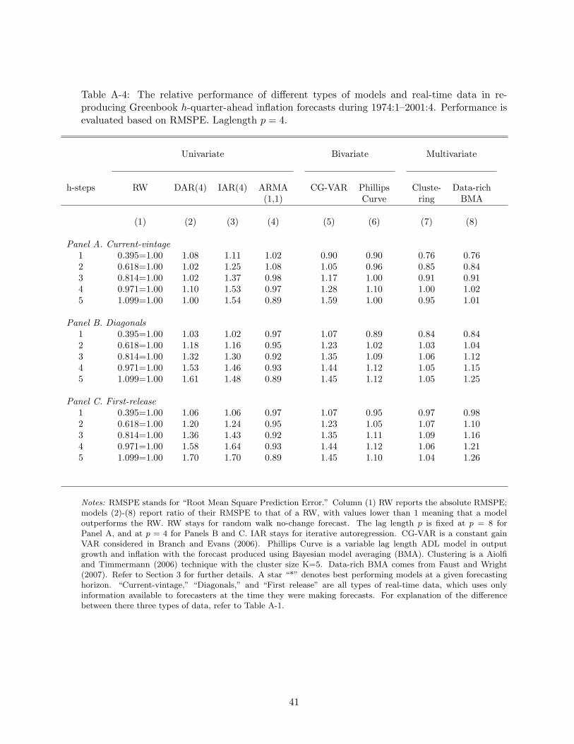
Table A-4: The relative performance of different types of models and real-time data in re-producing Greenbook h-quarter-ahead inflation forecasts during 1974:1–2001:4. Performance isevaluated based on RMSPE. Laglength p = 4.

Univariate Bivariate Multivariate

h-steps RW DAR(4) IAR(4) ARMA CG-VAR Phillips Cluste- Data-rich(1,1) Curve ring BMA

(1) (2) (3) (4) (5) (6) (7) (8)

Panel A. Current-vintage1 0.395=1.00 1.08 1.11 1.02 0.90 0.90 0.76 0.762 0.618=1.00 1.02 1.25 1.08 1.05 0.96 0.85 0.843 0.814=1.00 1.02 1.37 0.98 1.17 1.00 0.91 0.914 0.971=1.00 1.10 1.53 0.97 1.28 1.10 1.00 1.025 1.099=1.00 1.00 1.54 0.89 1.59 1.00 0.95 1.01

Panel B. Diagonals1 0.395=1.00 1.03 1.02 0.97 1.07 0.89 0.84 0.842 0.618=1.00 1.18 1.16 0.95 1.23 1.02 1.03 1.043 0.814=1.00 1.32 1.30 0.92 1.35 1.09 1.06 1.124 0.971=1.00 1.53 1.46 0.93 1.44 1.12 1.05 1.155 1.099=1.00 1.61 1.48 0.89 1.45 1.12 1.05 1.25

Panel C. First-release1 0.395=1.00 1.06 1.06 0.97 1.07 0.95 0.97 0.982 0.618=1.00 1.20 1.24 0.95 1.23 1.05 1.07 1.103 0.814=1.00 1.36 1.43 0.92 1.35 1.11 1.09 1.164 0.971=1.00 1.58 1.64 0.93 1.44 1.12 1.06 1.215 1.099=1.00 1.70 1.70 0.89 1.45 1.10 1.04 1.26

Notes: RMSPE stands for “Root Mean Square Prediction Error.” Column (1) RW reports the absolute RMSPE;models (2)-(8) report ratio of their RMSPE to that of a RW, with values lower than 1 meaning that a modeloutperforms the RW. RW stays for random walk no-change forecast. The lag length p is fixed at p = 8 forPanel A, and at p = 4 for Panels B and C. IAR stays for iterative autoregression. CG-VAR is a constant gainVAR considered in Branch and Evans (2006). Phillips Curve is a variable lag length ADL model in outputgrowth and inflation with the forecast produced using Bayesian model averaging (BMA). Clustering is a Aiolfiand Timmermann (2006) technique with the cluster size K=5. Data-rich BMA comes from Faust and Wright(2007). Refer to Section 3 for further details. A star “*” denotes best performing models at a given forecastinghorizon. “Current-vintage,” “Diagonals,” and “First release” are all types of real-time data, which uses onlyinformation available to forecasters at the time they were making forecasts. For explanation of the differencebetween there three types of data, refer to Table A-1.

41

Table A-5: Relative performance of different types of models and real-time data in reproducingGreenbook h-quarter-ahead inflation forecast during 1974:1-2001:4. Performance is evaluatedbased on RMSPE. Laglength p = 8.

Univariate Bivariate Multivariate

h-steps RW DAR(8) IAR(8) ARMA CG-VAR Phillips Cluste- Data-rich(1,1) Curve ring BMA

(1) (2) (3) (4) (5) (6) (7) (8)

Panel A. Current-vintage1 0.395=1.00 0.76 0.75 1.02 0.86 0.79 0.76 0.802 0.618=1.00 0.85 0.85 1.08 1.12 0.84 0.87 0.923 0.814=1.00 0.91 0.91 0.98 1.28 0.87 0.91 0.984 0.971=1.00 1.05 1.00 0.97 1.50 0.95 1.00 1.145 1.099=1.00 1.03 0.95 0.89 1.56 0.84 0.95 1.10

Panel B. Diagonals1 0.395=1.00 1.01 1.00 0.97 1.35 0.93 0.84 0.982 0.618=1.00 1.39 1.25 0.95 1.49 1.20 1.03 1.393 0.814=1.00 1.74 1.45 0.92 1.65 1.40 1.06 1.774 0.971=1.00 2.23 1.72 0.93 1.76 1.51 1.05 2.195 1.099=1.00 2.57 1.78 0.89 1.88 1.57 1.05 2.43

Panel C. First-release1 0.395=1.00 1.13 1.13 0.97 1.35 1.04 0.97 1.122 0.618=1.00 1.33 1.31 0.95 1.49 1.23 1.07 1.373 0.814=1.00 1.70 1.56 0.92 1.65 1.40 1.09 1.844 0.971=1.00 2.17 1.86 0.93 1.76 1.47 1.06 2.225 1.099=1.00 2.51 2.01 0.89 1.88 1.53 1.04 2.47

Notes: RMSPE stays for “Root Mean Square Prediction Error.” First column (1) RW reports absolute RMSPE;models (2)-(8) report ratio of their RMSPE to that of a RW, with values lower than 1 meaning that a modeloutperforms the RW RW stays for random walk no-change forecast. IAR stays for iterative autoregression. CG-VAR is a constant gain VAR considered in Branch and Evans (2006). Phillips Curve is a variable lag lengthPhillips curve model in output growth and inflation with a forecast produced using Bayesian model averaging(BMA). Clustering is a Aiolfi and Timmermann (2006) technique with cluster size K=5. Data-rich BMA comesfrom Faust and Wright (2007). Refer to Section 3 for further details. Star “*” denotes the best performing modelat a given forecasting horizon. “Current-vintage,” “Diagonals,” and “First release” are all types of real-time data,which uses only information available to forecasters at the time they were making forecasts. For explanation ofdifferences between there three types of data, refer to Table A-1.

42

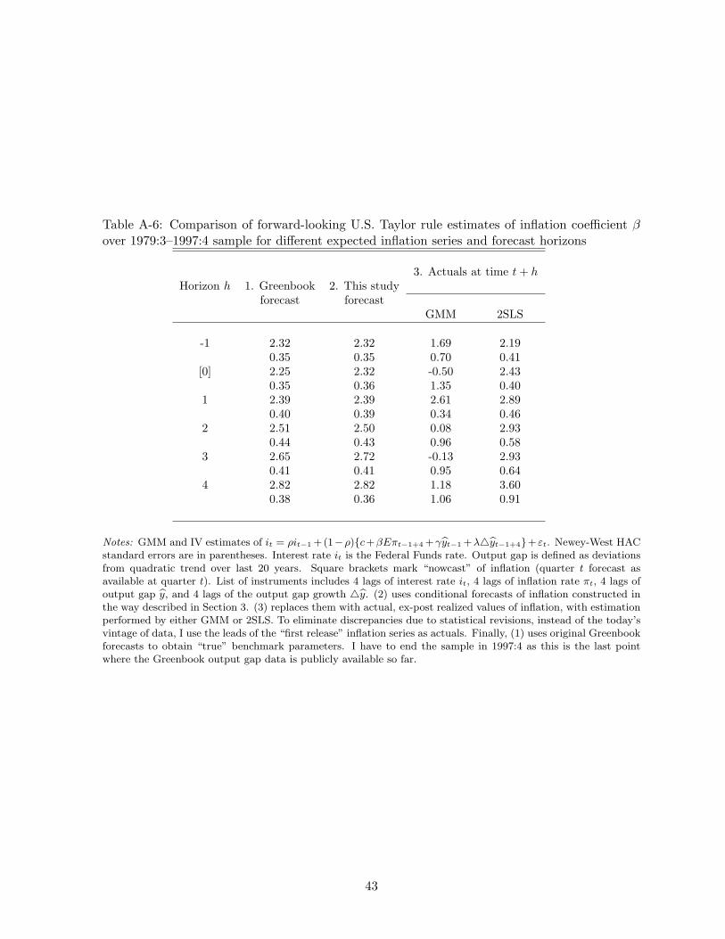
Table A-6: Comparison of forward-looking U.S. Taylor rule estimates of inflation coefficient βover 1979:3–1997:4 sample for different expected inflation series and forecast horizons

3. Actuals at time t+ hHorizon h 1. Greenbook 2. This study

forecast forecastGMM 2SLS

-1 2.32 2.32 1.69 2.190.35 0.35 0.70 0.41

[0] 2.25 2.32 -0.50 2.430.35 0.36 1.35 0.40

1 2.39 2.39 2.61 2.890.40 0.39 0.34 0.46

2 2.51 2.50 0.08 2.930.44 0.43 0.96 0.58

3 2.65 2.72 -0.13 2.930.41 0.41 0.95 0.64

4 2.82 2.82 1.18 3.600.38 0.36 1.06 0.91

Notes: GMM and IV estimates of it = ρit−1 +(1−ρ)c+βEπt−1+4 +γyt−1 +λ4yt−1+4+εt. Newey-West HACstandard errors are in parentheses. Interest rate it is the Federal Funds rate. Output gap is defined as deviationsfrom quadratic trend over last 20 years. Square brackets mark “nowcast” of inflation (quarter t forecast asavailable at quarter t). List of instruments includes 4 lags of interest rate it, 4 lags of inflation rate πt, 4 lags ofoutput gap y, and 4 lags of the output gap growth 4y. (2) uses conditional forecasts of inflation constructed inthe way described in Section 3. (3) replaces them with actual, ex-post realized values of inflation, with estimationperformed by either GMM or 2SLS. To eliminate discrepancies due to statistical revisions, instead of the today’svintage of data, I use the leads of the “first release” inflation series as actuals. Finally, (1) uses original Greenbookforecasts to obtain “true” benchmark parameters. I have to end the sample in 1997:4 as this is the last pointwhere the Greenbook output gap data is publicly available so far.

43

Table A-7: Canadian real-time Taylor rule estimates over 1991:1–2007:1

Gap: Window Quadratic HP Band-pass

(1) (2) (3) (4)

Panel A. Backward-looking Taylor rule (h = 0)Inflation β 0.28 0.27 0.36 0.36

0.29 0.28 0.38 0.39Output gap γ -0.26 -0.24 -0.29 -0.37

0.10 0.09 0.41 0.44Const c 3.75 4.83 3.67 3.62

0.65 0.82 0.80 0.79R2 0.31 0.32 0.12 0.13

Panel B. Forward-looking Taylor rule (h = 10)Inflation forecast β 1.14 1.13 1.27 1.26

0.20 0.20 0.21 0.23Output gap γ -0.26 -0.24 -0.75 -0.87

0.06 0.06 0.25 0.29Const c 1.34 2.44 0.82 0.77

0.57 0.69 0.65 0.68R2 0.63 0.64 0.52 0.52

Notes: Least squares estimates of it = c + βEπt−2+h + γyt−2 + εt. Newey-West HAC standard errors are inparentheses. Expectations are formed using “current vintage” data. See Table A-1 for details. Interest rate itis the middle month overnight rate. Inflation is the core CPI year-over-year inflation rate. “Window” assumesquadratic detrending over last 20 years.

44

Table A-8: German real-time backward-looking Taylor rule estimates over 1979:1–1998:4

Variable Specification

(1) (2) (3) (4) (5) (6)

Inflation β 0.78 1.19 1.17 1.23 1.34 1.380.23 0.27 0.49 0.10 0.10 0.14

Output gap γ 0.95 0.99 0.79 0.51 0.51 0.220.16 0.29 0.37 0.05 0.06 0.07

Real exchange rate ξ 0.05 0.08 0.05 0.050.02 0.03 0.01 0.01

Federal Funds Rate λ 0.41 0.100.12 0.07

Smoothing ρ 0.79 0.80 0.870.04 0.06 0.06

Const c -0.98 -1.50 5.14 -0.73 -0.84 2.891.34 2.12 1.86 0.72 0.84 0.42

R2 0.96 0.95 0.94 0.79 0.78 0.68

Notes: NLLS estimates of it = ρit−1+(1−ρ)c+βEπt−1+γyt−1+ξ4Et+λrUSt +εt. Newey-West HAC standarderrors are in parentheses. Interest rate it is the Money Market Rate. Output gap is real-time Bundesbank’sestimates of the output gap.

45

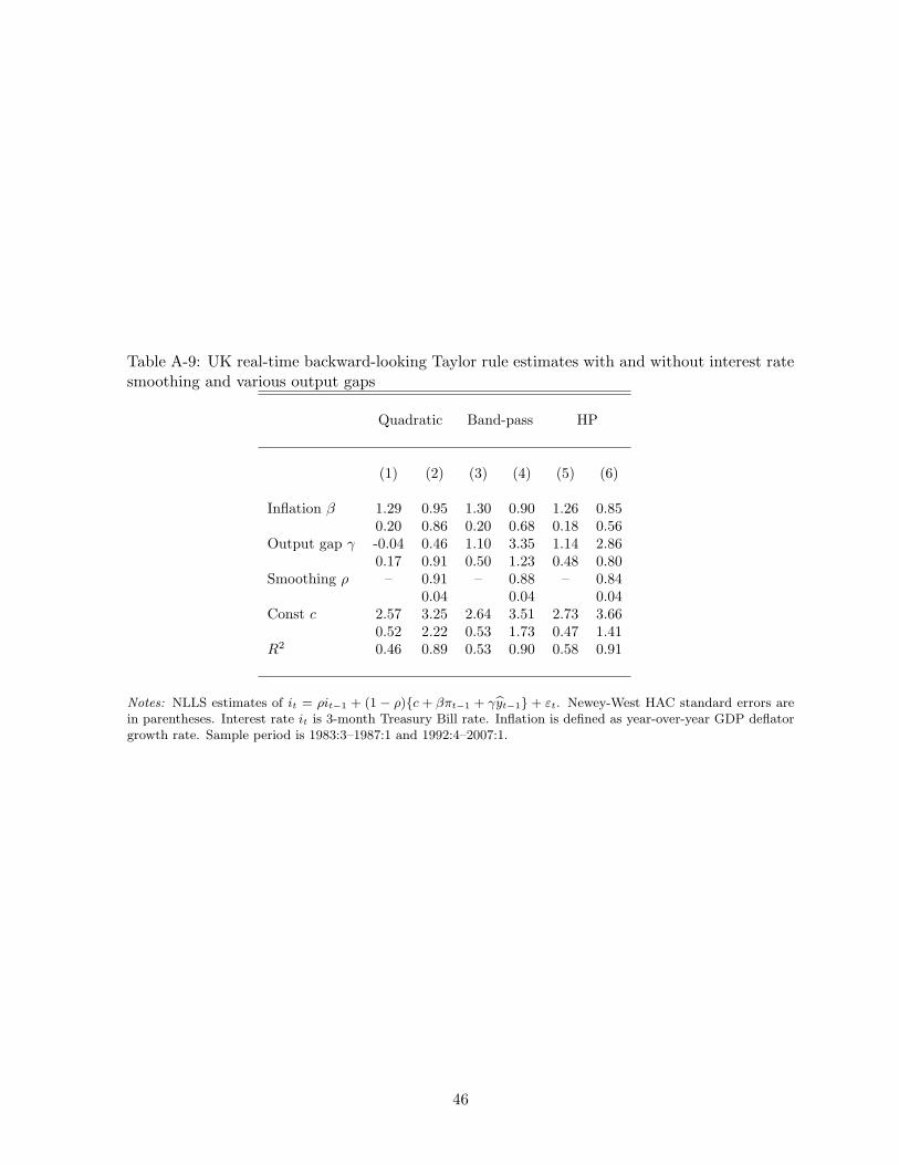
Table A-9: UK real-time backward-looking Taylor rule estimates with and without interest ratesmoothing and various output gaps

Quadratic Band-pass HP

(1) (2) (3) (4) (5) (6)

Inflation β 1.29 0.95 1.30 0.90 1.26 0.850.20 0.86 0.20 0.68 0.18 0.56

Output gap γ -0.04 0.46 1.10 3.35 1.14 2.860.17 0.91 0.50 1.23 0.48 0.80

Smoothing ρ – 0.91 – 0.88 – 0.840.04 0.04 0.04

Const c 2.57 3.25 2.64 3.51 2.73 3.660.52 2.22 0.53 1.73 0.47 1.41

R2 0.46 0.89 0.53 0.90 0.58 0.91

Notes: NLLS estimates of it = ρit−1 + (1 − ρ)c + βπt−1 + γyt−1 + εt. Newey-West HAC standard errors arein parentheses. Interest rate it is 3-month Treasury Bill rate. Inflation is defined as year-over-year GDP deflatorgrowth rate. Sample period is 1983:3–1987:1 and 1992:4–2007:1.

46

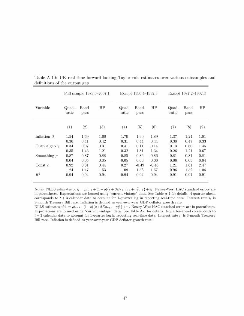
Table A-10: UK real-time forward-looking Taylor rule estimates over various subsamples anddefinitions of the output gap

Full sample 1983:3–2007:1 Except 1990:4–1992:3 Except 1987:2–1992:3

Variable Quad- Band- HP Quad- Band- HP Quad- Band- HPratic pass ratic pass ratic pass

(1) (2) (3) (4) (5) (6) (7) (8) (9)

Inflation β 1.54 1.69 1.66 1.70 1.90 1.89 1.37 1.24 1.010.36 0.41 0.42 0.31 0.44 0.44 0.30 0.47 0.33

Output gap γ 0.34 0.07 0.31 0.41 0.11 0.14 0.13 0.60 1.450.35 1.43 1.21 0.32 1.81 1.34 0.26 1.21 0.67

Smoothing ρ 0.87 0.87 0.88 0.85 0.86 0.86 0.81 0.81 0.810.04 0.05 0.05 0.05 0.06 0.06 0.06 0.05 0.04

Const c 0.92 0.31 0.44 0.27 -0.49 -0.46 1.21 1.61 2.471.24 1.47 1.53 1.09 1.53 1.57 0.96 1.52 1.06

R2 0.94 0.94 0.94 0.94 0.94 0.94 0.91 0.91 0.91

Notes: NLLS estimates of it = ρit−1 + (1−ρ)c+βEπt−1+4 +γyt−1+ εt. Newey-West HAC standard errors arein parentheses. Expectations are formed using “current vintage” data. See Table A-1 for details. 4-quarter-aheadcorresponds to t + 3 calendar date to account for 1-quarter lag in reporting real-time data. Interest rate it is3-month Treasury Bill rate. Inflation is defined as year-over-year GDP deflator growth rate.NLLS estimates of it = ρit−1+(1−ρ)c+βEπt+h+γyt+εt. Newey-West HAC standard errors are in parentheses.Expectations are formed using “current vintage” data. See Table A-1 for details. 4-quarter-ahead corresponds tot+ 3 calendar date to account for 1-quarter lag in reporting real-time data. Interest rate it is 3-month TreasuryBill rate. Inflation is defined as year-over-year GDP deflator growth rate.

47

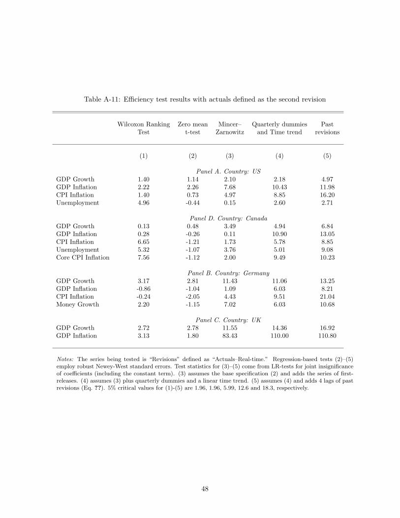
Table A-11: Efficiency test results with actuals defined as the second revision

Wilcoxon Ranking Zero mean Mincer– Quarterly dummies PastTest t-test Zarnowitz and Time trend revisions

(1) (2) (3) (4) (5)

Panel A. Country: USGDP Growth 1.40 1.14 2.10 2.18 4.97GDP Inflation 2.22 2.26 7.68 10.43 11.98CPI Inflation 1.40 0.73 4.97 8.85 16.20Unemployment 4.96 -0.44 0.15 2.60 2.71

Panel D. Country: CanadaGDP Growth 0.13 0.48 3.49 4.94 6.84GDP Inflation 0.28 -0.26 0.11 10.90 13.05CPI Inflation 6.65 -1.21 1.73 5.78 8.85Unemployment 5.32 -1.07 3.76 5.01 9.08Core CPI Inflation 7.56 -1.12 2.00 9.49 10.23

Panel B. Country: GermanyGDP Growth 3.17 2.81 11.43 11.06 13.25GDP Inflation -0.86 -1.04 1.09 6.03 8.21CPI Inflation -0.24 -2.05 4.43 9.51 21.04Money Growth 2.20 -1.15 7.02 6.03 10.68

Panel C. Country: UKGDP Growth 2.72 2.78 11.55 14.36 16.92GDP Inflation 3.13 1.80 83.43 110.00 110.80

Notes: The series being tested is “Revisions” defined as “Actuals–Real-time.” Regression-based tests (2)–(5)employ robust Newey-West standard errors. Test statistics for (3)–(5) come from LR-tests for joint insignificanceof coefficients (including the constant term). (3) assumes the base specification (2) and adds the series of first-releases. (4) assumes (3) plus quarterly dummies and a linear time trend. (5) assumes (4) and adds 4 lags of pastrevisions (Eq. ??). 5% critical values for (1)-(5) are 1.96, 1.96, 5.99, 12.6 and 18.3, respectively.

48

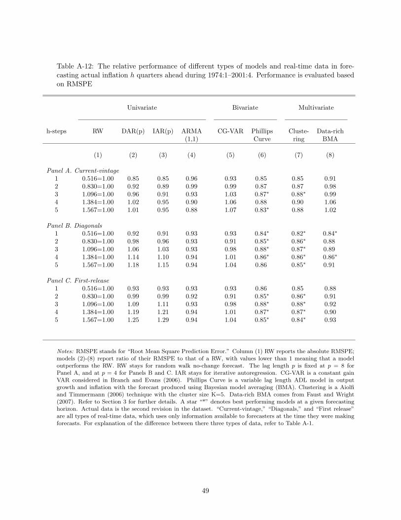
Table A-12: The relative performance of different types of models and real-time data in fore-casting actual inflation h quarters ahead during 1974:1–2001:4. Performance is evaluated basedon RMSPE

Univariate Bivariate Multivariate

h-steps RW DAR(p) IAR(p) ARMA CG-VAR Phillips Cluste- Data-rich(1,1) Curve ring BMA

(1) (2) (3) (4) (5) (6) (7) (8)

Panel A. Current-vintage1 0.516=1.00 0.85 0.85 0.96 0.93 0.85 0.85 0.912 0.830=1.00 0.92 0.89 0.99 0.99 0.87 0.87 0.983 1.096=1.00 0.96 0.91 0.93 1.03 0.87∗ 0.88∗ 0.994 1.384=1.00 1.02 0.95 0.90 1.06 0.88 0.90 1.065 1.567=1.00 1.01 0.95 0.88 1.07 0.83∗ 0.88 1.02

Panel B. Diagonals1 0.516=1.00 0.92 0.91 0.93 0.93 0.84∗ 0.82∗ 0.84∗

2 0.830=1.00 0.98 0.96 0.93 0.91 0.85∗ 0.86∗ 0.883 1.096=1.00 1.06 1.03 0.93 0.98 0.88∗ 0.87∗ 0.894 1.384=1.00 1.14 1.10 0.94 1.01 0.86∗ 0.86∗ 0.86∗

5 1.567=1.00 1.18 1.15 0.94 1.04 0.86 0.85∗ 0.91

Panel C. First-release1 0.516=1.00 0.93 0.93 0.93 0.93 0.86 0.85 0.882 0.830=1.00 0.99 0.99 0.92 0.91 0.85∗ 0.86∗ 0.913 1.096=1.00 1.09 1.11 0.93 0.98 0.88∗ 0.88∗ 0.924 1.384=1.00 1.19 1.21 0.94 1.01 0.87∗ 0.87∗ 0.905 1.567=1.00 1.25 1.29 0.94 1.04 0.85∗ 0.84∗ 0.93

Notes: RMSPE stands for “Root Mean Square Prediction Error.” Column (1) RW reports the absolute RMSPE;models (2)-(8) report ratio of their RMSPE to that of a RW, with values lower than 1 meaning that a modeloutperforms the RW. RW stays for random walk no-change forecast. The lag length p is fixed at p = 8 forPanel A, and at p = 4 for Panels B and C. IAR stays for iterative autoregression. CG-VAR is a constant gainVAR considered in Branch and Evans (2006). Phillips Curve is a variable lag length ADL model in outputgrowth and inflation with the forecast produced using Bayesian model averaging (BMA). Clustering is a Aiolfiand Timmermann (2006) technique with the cluster size K=5. Data-rich BMA comes from Faust and Wright(2007). Refer to Section 3 for further details. A star “*” denotes best performing models at a given forecastinghorizon. Actual data is the second revision in the dataset. “Current-vintage,” “Diagonals,” and “First release”are all types of real-time data, which uses only information available to forecasters at the time they were makingforecasts. For explanation of the difference between there three types of data, refer to Table A-1.

49