Estimated Effects of Speculation & Interest Rates in a “Carry Trade”

Model of Commodity Prices

Jeffrey FrankelHarpel Professor, Harvard University

SESSION VI. FORECASTING COMMODITY PRICES

in Understanding International Commodity Price Fluctuations

International Conference organized by the IMF's Research Department and the Oxford Centre

for the Analysis of Resource Rich Economies at Oxford University.

March 20-21, 2013Washington, D.C

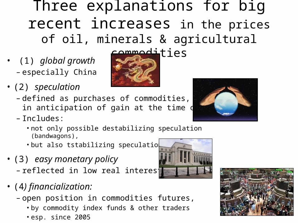
Three explanations for big recent increases in the prices of oil, minerals & agricultural commodities

• (1) global growth– especially China

• (2) speculation– defined as purchases of commodities,

in anticipation of gain at the time of resale. – Includes:

• not only possible destabilizing speculation (bandwagons), • but also tstabilizing speculation.

• (3) easy monetary policy– reflected in low real interest rates.

• (4) financialization:– open position in commodities futures,

• by commodity index funds & other traders• esp. since 2005

High real interest rates reduce the price of storable commodities through 4 channels:

• ¤ by increasing the incentive for extraction today – rather than tomorrow; – think of rates at which oil is pumped, copper mined, or forests logged.

• ¤ by decreasing firms' desire to carry inventories; – think of oil inventories held in tanks.

• ¤ by encouraging speculators to shift out of spot commodity contracts, and into treasury bills, – the famous “financialization" of commodities.

• ¤ by appreciating the domestic currency – and so reducing the price of internationally traded commodities

in domestic terms, – even if the price hasn't fallen in terms of foreign currency.

Figure 1a: Real commodity price index (Moody’s) and real interest rates

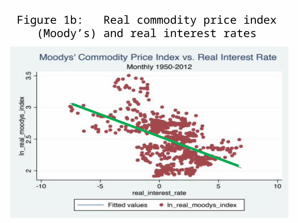
Figure 1b: Real commodity price index (Moody’s) and real interest rates

The 2008 spike in commodity prices

• Explanation (1) didn’t fit:– Growth had already begun to slow by 2008 1st half– while the commodity price rise accelerated.

• Explanation (4) couldn’t explain a sudden rise in 2008.

• That leaves explanations (2) & (3):– Speculation & low interest rates.

• But many argued that inventory data belied them:– if speculators were betting on future price increases,

inventory demand should be high.– The same if the cause were low interest rates.– But, it was claimed, inventory levels were not high.– E.g.. Kohn (2008), Krugman (2008a, b) & Wolf (2008).

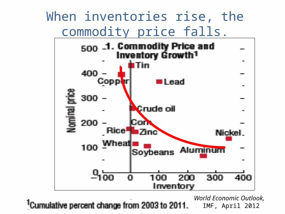
When inventories rise, the commodity price falls.

World Economic Outlook, IMF, April 2012

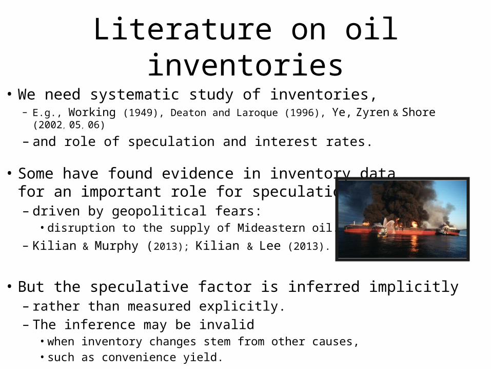
Literature on oil inventories• We need systematic study of inventories,

– E.g., Working (1949), Deaton and Laroque (1996), Ye, Zyren & Shore (2002, 05, 06)

– and role of speculation and interest rates.

• Some have found evidence in inventory data for an important role for speculation, – driven by geopolitical fears:

• disruption to the supply of Mideastern oil.

– Kilian & Murphy (2013); Kilian & Lee (2013).

• But the speculative factor is inferred implicitly – rather than measured explicitly.– The inference may be invalid

• when inventory changes stem from other causes, • such as convenience yield.

Empirical innovations of this paper

• Relative to past attempts to capture the roles of speculation or interest rates via inventories:

– How to measure speculation, market expectations of future commodity price changes?

• Survey data collected by Consensus Forecasts• from “over 30 of the world's most

prominent commodity forecasters.”

– How to measure perceived risk to commodity availability?• Volatility implicit in options prices.

1st assumption: regressive expectationsThis specification of expectations can be shown to be rational, in a model of sticky prices and the right value of ϑ. (Frankel, 1986.)

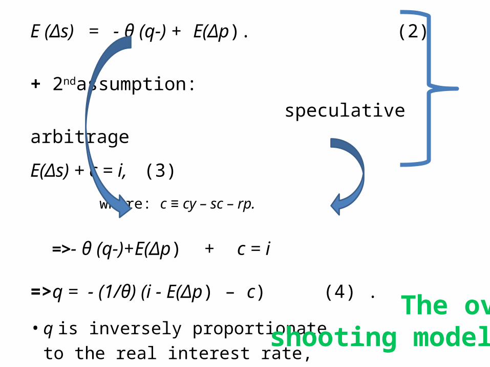
E (Δs) = - θ (q-) + E(Δp). (2)

+ 2ndassumption:

speculative arbitrage

E(Δs) + c = i, (3)

where: c ≡ cy – sc – rp.

=>- θ (q-)+E(Δp) + c = i

=>q = - (1/θ) (i - E(Δp) – c) (4) .

• q is inversely proportionate

to the real interest rate,

– ifand c are constant.

The over-shooting model

Regression of real commodity price indices against real interest rate

(1950-2012)Table 1 Dependent variable:

log of commodity price index, deflated by US CPI

VARIABLESCRB

indexDow Jones

IndexMoody’s

index

Goldman Sachs Index

Real interest rate -0.041*** -0.034*** -0.071** -0.075*** (0.007) (0.006) (0.005) (0.007)Constant 0.900*** 0.066*** 2.533*** 0.732***

(0.017) (0.016) (0.011) (0.018) Observations 739 739 739 513 R2 0.04 0.04 0.25 0.18

*** p<0.01 (Standard errors in parentheses.)

q is inversely proportionate to the real interest rate

The overshooting model

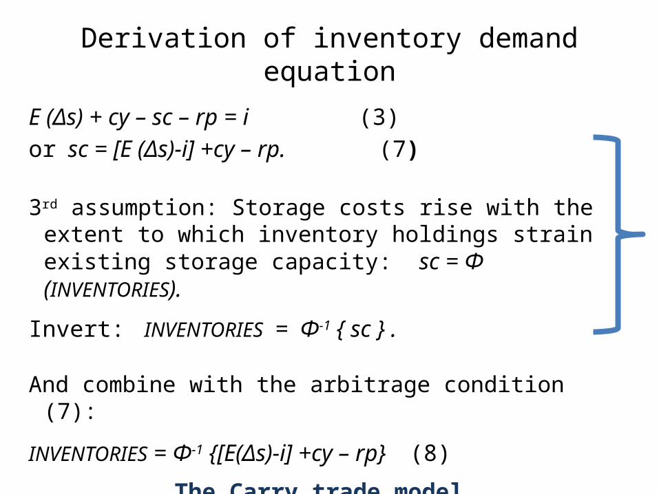
Derivation of inventory demand equation

E (Δs) + cy – sc – rp = i (3)

or sc = [E (Δs)-i] +cy – rp. (7)

3rd assumption: Storage costs rise with the extent to which inventory holdings strain existing storage capacity: sc = Φ (INVENTORIES).

Invert: INVENTORIES = Φ-1 { sc } .

And combine with the arbitrage condition (7):

INVENTORIES = Φ-1 {[E(Δs)-i] +cy – rp} (8)

The Carry trade model

Petroleum stocks Millions of barrels (3) (4) (1) (2)

Carry trade: EΔs - i 0.12*** 0.12*** 0.02* 0.02*(0.03) (0.03) (0.01) (0.01)

Actual US IP growth 0.56*** 0.56*** 0.02 0.01(0.15) (0.15) (0.08) (0.08)

US Industrial Prod. log -0.01 0.01

(0.07) (0.04)

Forecast 2-yr IP growth -0.674** -0.671** 0.003 0.000(0.318) (0.318) (0.146) (0.146)

Oil Stocks lagged log 0.91*** 0.91***(0.05) (0.05)

Trend 0.004*** 0.004*** 0.000 0.000

(0.000) (0.000) (0.000) (0.000)

Constant 7.313*** 7.356*** 0.653 0.600

(0.008) (0.316) (0.392) (0.481)

R2 0.84 0.84 0.97 0.97

Table 4 -- Oil Inventory Equation (1995-2011) 58 observations, quarterly

Complete equation for determination of price There is no reason for the net convenience yield, c, to be constant.

c ≡ cy – sc – rp (3) q- = - (1/θ) (i - E(Δp) – c) (4)

Substituting from (3) into (4),

q = - (1/θ) [i-E(Δp)] + (1/θ) cy - (1/θ) sc - (1/θ) rp (5)

Hypothesized effects:– Real interest rate: negative– Convenience yield: positive

• Economic activity• Risk of disruption

– Storage costs: negative• sc = Φ (INVENTORIES).

– Risk premium• Measured directly: [E(Δs)-(f-s)] • Or as determined by volatility σ: ambiguous

– Measured by actual volatility– Or option-implied subjective volatility

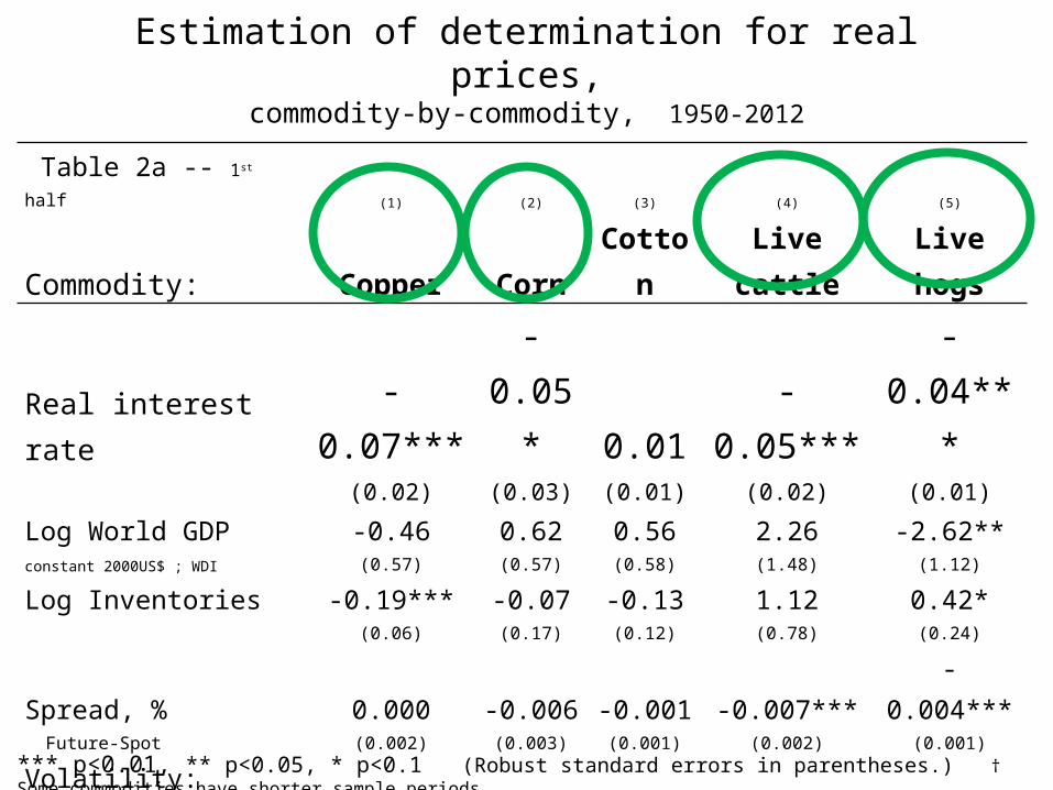
Estimation of determination for real prices,commodity-by-commodity, 1950-2012

 Table 2a -- 1st half (1) (2) (3) (4) (5)

Commodity: Copper Corn Cotton Live cattle Live hogs

Real interest rate -0.07*** -0.05* 0.01 -0.05*** -0.04***(0.02) (0.03) (0.01) (0.02) (0.01)

Log World GDP -0.46 0.62 0.56 2.26 -2.62**constant 2000US$ ; WDI (0.57) (0.57) (0.58) (1.48) (1.12)

Log Inventories -0.19*** -0.07 -0.13 1.12 0.42*(0.06) (0.17) (0.12) (0.78) (0.24)

Spread, % 0.000 -0.006 -0.001 -0.007*** -0.004*** Future-Spot (0.002) (0.003) (0.001) (0.002) (0.001)

Volatility: Std.dev. 3.04*** 0.94 0.20 -0.27 -1.02of log price over past year (0.72) (0.91) (0.53) (0.78) (0.61)

Linear trend -0.00 -0.04** -0.04* -0.08* 0.05(0.02) (0.02) (0.02) (0.04) (0.03)

Constant 16.94 -20.26 -14.94 -81.65 74.87**(17.29) (16.54) (17.29) (51.77) (33.00)

Observations (annual) † 50 51 51 32 39R2 0.55 0.66 0.76 0.51 0.80

*** p<0.01, ** p<0.05, * p<0.1 (Robust standard errors in parentheses.) † Some commodities have shorter sample periods.

Estimation of determination for real prices,commodity-by-commodity, 1950-2012, continued

*** p<0.01, ** p<0.05, * p<0.1 (Robust standard errors in parentheses.) † Some commodities have shorter sample periods.

 Table 2a -- 2nd half (6) (7) (8) (9) (10) (11)

Commodity: Oats Petroleum Platinum Silver Soybeans Wheat

Real interest rate -0.04** -0.02 0.08*** -0.02 -0.04** -0.003(0.016) (0.071) (0.015) (0.025) (0.016) (0.021)

Log World GDP 1.56** -4.42 3.38*** 3.63* 0.38 0.33(constant 2000 US$);WDI (0.593) (4.984) (0.753) (2.012) (0.837) (0.702)

Log Inventories -0.31** -2.82 -0.24*** 0.01 0.04 -0.45*(0.13) (4.43) (0.03) (0.11) (0.09) (0.24)

Spread, % -0.015* -0.002 -0.000 -0.010** -0.007** -0.001 Future-Spot (0.003) (0.003) (0.001) (0.004) (0.003) (0.003)

Volatility: Std.dev. 0.91 -0.08 1.10*** 5.15*** 1.86** 1.81***of log price over past year (0.66) (0.69) (0.36) (0.67) (0.87) (0.65)

Linear trend -0.09*** 0.17 -0.12*** -0.12* -0.04 -0.03(0.03) (0.14) (0.03) (0.06) (0.03) (0.02)

Constant -45.54*** 156.65 -98.36*** -111.77* -13.65 -7.09(16.33) (142.65) (22.41) (60.57) (24.71) (20.18)

Observations (annual) 50 29 47 44 48 51R2 0.63 0.34 0.73 0.62 0.71 0.74

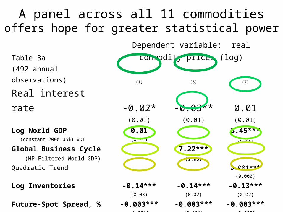
A panel across all 11 commoditiesoffers hope for greater statistical power

Table 3a Dependent variable: real commodity prices (log)(492 annual observations) (1) (6) (7)

Real interest rate -0.02* -0.03** 0.01(0.01) (0.01) (0.01)

Log World GDP 0.01 3.45*** (constant 2000 US$) WDI (0.24) (0.77)

Global Business Cycle 7.22*** (HP-Filtered World GDP) (1.08)

Quadratic Trend 0.001***(0.000)

Log Inventories -0.14*** -0.14*** -0.13***(0.03) (0.02) (0.02)

Future-Spot Spread, % -0.003*** -0.003*** -0.003***(0.001) (0.001) (0.000)

Volatility: Standard deviation 1.81*** 1.92*** 1.77*** of log spot price of past year (0.52) (0.51) (0.47)

Linear Trend -0.02* -0.02*** -0.19***(0.01) (0.00) (0.04)

Constant 0.01 0.32 -101.90***(7.01) (0.23) (22.93)

R2 0.46 0.49 0.51

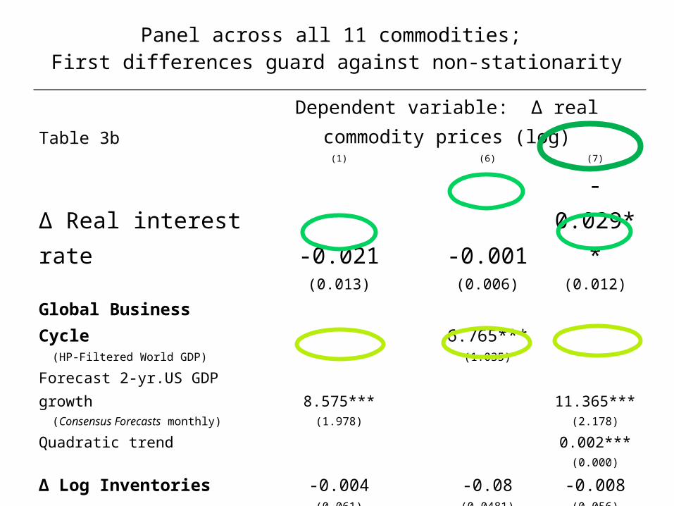
Panel across all 11 commodities; First differences guard against non-stationarity

Table 3b Dependent variable: Δ real commodity prices (log)(1) (6) (7)

Δ Real interest rate -0.021 -0.001 -0.029**(0.013) (0.006) (0.012)

Global Business Cycle 6.765*** (HP-Filtered World GDP) (1.035)

Forecast 2-yr.US GDP growth 8.575*** 11.365*** (Consensus Forecasts monthly) (1.978) (2.178)

Quadratic trend 0.002***(0.000)

Δ Log Inventories -0.004 -0.08 -0.008(0.061) (0.0481) (0.056)

Δ Future-Spot Spread, % -0.001*** -0.002*** -0.002***(0.000) (0.0005) (0.000)

Δ Volatility: Std.dev. of -0.067 0.192 0.068 log spot price of past year (0.184) (0.213) (0.208)

Linear Trend 0.010*** 0.002*** -0.024***

(0.002) (0.000) (0.005)

Constant -0.314*** -0.043*** -0.271***

(0.068) (0.009) (0.071)

Observations 216 486 216

R2 0.22 0.17 0.27

In conclusion…

• The model can accommodate each of the explanations for recent increases in commodity prices: economic activity, speculation, and easy monetary policy. – Based on “carry trade”: arbitrage relationship between expected price

change and costs of carry: interest rate, storage costs, and convenience yield.

– And on “overshooting”: prices are expected to regress gradually back to long-run equilibrium

• Specialized data sources:– Inventory holdings, as a determinant of storage costs;– Survey data on forecasts,

as a measure of market expectations of future prices;– Option-implied volatility, as a measure of risk perceptions,

• to supplement actual volatility

Empirical findings

• Support for Carry Trade approach:– Negative effect of inventory levels on commodity price;– Negative effect of interest rate

• on inventory demand and so on commodity price;

– Positive effect of expected price increase • on inventory demand and so on commodity price.

• More specifically, the overshooting model:– negative effect of real interest rate on real commodity prices.

• Also some (limited) support for other relevant variables:– economic activity– forward-spot spread– volatility.

22

Appendix: Data graphsReal Moody’s commodity price index

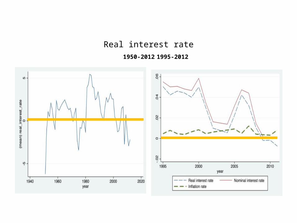
Real interest rate 1950-2012 1995-2012

Petroleum inventories

Risk premium & 2 measures of volatility (f-s) - E(Δs) option-implied and actual volatilities

The disappearance of the positive risk premium after 2005 (EΔs measured by survey data) and with no obvious trend in volatility

is consistent with Hamilton &Wu’s (2013) interpretation of the financialization hypothesis:Investors in commodity indices took the long side of the futures market after 2005.

Spot prices of individual commoditieswith forward-spot spread

Minerals

Spot prices of individual commoditieswith forward-spot spread

Food crops

Spot prices of individual commoditieswith forward-spot spread

Other agricultural