fluid/structure coupled aeroelastic ...aero-comlab.stanford.edu/papers/doi.thesis.pdffluid/structure...
TRANSCRIPT

FLUID/STRUCTURE COUPLED AEROELASTIC
COMPUTATIONS FOR TRANSONIC FLOWS IN
TURBOMACHINERY
a dissertation
submitted to the department of aeronautics and astronautics
and the committee on graduate studies
of stanford university
in partial fulfillment of the requirements
for the degree of
doctor of philosophy
Hirofumi Doi
August 2002

c© Copyright by Hirofumi Doi 2002
All Rights Reserved
ii

I certify that I have read this dissertation and that in
my opinion it is fully adequate, in scope and quality, as
a dissertation for the degree of Doctor of Philosophy.
Juan J. Alonso(Principal Adviser)
I certify that I have read this dissertation and that in
my opinion it is fully adequate, in scope and quality, as
a dissertation for the degree of Doctor of Philosophy.
Antony Jameson
I certify that I have read this dissertation and that in
my opinion it is fully adequate, in scope and quality, as
a dissertation for the degree of Doctor of Philosophy.
Holt Ashley
I certify that I have read this dissertation and that in
my opinion it is fully adequate, in scope and quality, as
a dissertation for the degree of Doctor of Philosophy.
Roger L. Davis(University of California, Davis)
Approved for the University Committee on Graduate
Studies:
iii
Abstract
The unstable, self-excited or forced vibrations of rotor blades must be avoided in
designing high performance turbomachinery components because they may induce
catastrophic structural failures. In evaluating the stability of such vibrations, com-
putational approaches have been bearing an increasing role due to the surprising
progress of both computer technologies and advanced algorithms. They are now at a
stage where time domain fluid/structure coupled simulations of aeroelastic phenom-
ena in turbomachinery with realistic geometries can be used in practice. The present
study demonstrates the capabilities of a fluid/structure coupled computational ap-
proach which consists of an unsteady three-dimensional Navier-Stokes flow solver,
TFLO, a finite element structural analysis package, MSC/NASTRAN, and the cou-
pling interface between the two disciplines. The flow solver relies on a multiblock,
cell-centered finite volume discretization and the dual time stepping time integration
scheme with multigrid for convergence acceleration. Parallelization for multiple pro-
cessors is also performed to achieve faster computations making use of the Message
Passing Interface (MPI). As far as the interface is concerned, high accuracy is pursued
with respect to load transfer, deformation tracking and synchronization. As a result,
the program successfully predicts the aeroelastic responses of a high performance fan,
NASA Rotor 67, over a range of operational conditions. The major contribution to
the aerodynamic damping for turbomachinery blade motions is observed to be the
unsteady pressure generated at the location of the shock. The results show that the
iv

unsteady pressure may act to damp or excite the blade motion mainly depending on
the inter-blade phase angle. It is concluded that the level of fidelity in the individ-
ual disciplines, together with an accurate coupling interface will allow for accurate
prediction of flutter boundaries of turbomachinery components.
v

Acknowledgments
I would like to express my deepest gratitude to my advisor, Professor Juan Jose
Alonso for suggesting this project and providing guidance throughout the course of
this thesis. He has given me considerable freedom and shown patience as I pursued
the idea development in this project. I would also like to thank Professor Roger L.
Davis for many fruitful suggestions and for providing me with the computational grid
for Rotor 67. I would further like to thank the readers, Professor Antony Jameson and
Professor Holt Ashley, for taking the time to read this thesis, and making valuable
suggestions.
I thank my fellow students for useful discussions with them and various help
including computer support and my priority in using computer resources. I thank
the people involved in the TFLO development program for providing me with the up-
to-date sophisticated solver. I thank my friends for their encouragement which has
been a vital contribution to this work. I would also like to acknowledge the financial
support provided by the Japan Defense Agency.
vi

Contents
Abstract iv
Acknowledgments vi
1 Introduction 1
1.1 Description of the Problem . . . . . . . . . . . . . . . . . . . . . . . . 1
1.2 Past Efforts . . . . . . . . . . . . . . . . . . . . . . . . . . . . . . . . 7
1.2.1 Linearized Unsteady Aerodynamic Theory . . . . . . . . . . . 7
1.2.2 Time-Linearized Computations for Unsteady Aerodynamics . 11
1.2.3 Time-Marching Computations for Unsteady Aerodynamics . . 12
1.2.4 Fluid/Structure Coupled Computations . . . . . . . . . . . . . 15
1.3 Motivations of the Research . . . . . . . . . . . . . . . . . . . . . . . 17
2 Governing Equations 20
2.1 Unsteady Aerodynamics . . . . . . . . . . . . . . . . . . . . . . . . . 21
2.1.1 Reynolds’ Transport Theorem . . . . . . . . . . . . . . . . . . 22
2.1.2 Conservation of Mass . . . . . . . . . . . . . . . . . . . . . . . 22
2.1.3 Conservation of Momentum . . . . . . . . . . . . . . . . . . . 23
2.1.4 Conservation of Energy . . . . . . . . . . . . . . . . . . . . . . 25
2.1.5 The Reynolds-Averaged Navier Stokes Equations . . . . . . . 27
2.1.6 Conservation Law Form . . . . . . . . . . . . . . . . . . . . . 29
2.2 Structural Mechanics . . . . . . . . . . . . . . . . . . . . . . . . . . . 31
2.2.1 Differential Equations of Elasticity . . . . . . . . . . . . . . . 32
2.2.2 The Principle of Virtual Work . . . . . . . . . . . . . . . . . . 34
vii

2.3 Fluid/Structure Interaction . . . . . . . . . . . . . . . . . . . . . . . 35
2.3.1 Conservation of Loads and Energy . . . . . . . . . . . . . . . 35
2.3.2 Geometric Conservation Law . . . . . . . . . . . . . . . . . . . 36
3 Description of the Method 39
3.1 Unsteady Aerodynamics . . . . . . . . . . . . . . . . . . . . . . . . . 40
3.1.1 Cell-Centered Finite Volume Scheme . . . . . . . . . . . . . . 43
3.1.2 Artificial Dissipation . . . . . . . . . . . . . . . . . . . . . . . 45
3.1.3 Dual Time Stepping . . . . . . . . . . . . . . . . . . . . . . . 47
3.1.4 Time Marching Scheme . . . . . . . . . . . . . . . . . . . . . . 50
3.1.5 Multigrid . . . . . . . . . . . . . . . . . . . . . . . . . . . . . 52
3.1.6 Boundary Conditions . . . . . . . . . . . . . . . . . . . . . . . 54
3.1.7 Turbulence Model . . . . . . . . . . . . . . . . . . . . . . . . . 61
3.1.8 Moving Mesh System . . . . . . . . . . . . . . . . . . . . . . . 64
3.2 Structural Mechanics . . . . . . . . . . . . . . . . . . . . . . . . . . . 71
3.2.1 Finite Element Analysis . . . . . . . . . . . . . . . . . . . . . 72
3.2.2 Finite Element Model . . . . . . . . . . . . . . . . . . . . . . 75
3.2.3 Damping Characteristics . . . . . . . . . . . . . . . . . . . . . 76
3.2.4 Centrifugal and Coriolis Forces . . . . . . . . . . . . . . . . . 78
3.2.5 Time Integration . . . . . . . . . . . . . . . . . . . . . . . . . 81
3.3 Fluid-Structure Interface . . . . . . . . . . . . . . . . . . . . . . . . . 83
3.3.1 Deformation Tracking System . . . . . . . . . . . . . . . . . . 84
3.3.2 Load Transfer System . . . . . . . . . . . . . . . . . . . . . . 88
3.3.3 Synchronization . . . . . . . . . . . . . . . . . . . . . . . . . . 90
3.4 Parallelization . . . . . . . . . . . . . . . . . . . . . . . . . . . . . . . 93
3.4.1 Flow Solver . . . . . . . . . . . . . . . . . . . . . . . . . . . . 94
3.4.2 Structural Solver . . . . . . . . . . . . . . . . . . . . . . . . . 96
4 Results 97
4.1 Code Evaluation - Cantilever Double Circular Arc Airfoil Wing . . . 97
4.2 Flutter Analysis Demonstration - NASA Rotor 67 . . . . . . . . . . . 105
4.2.1 NASA Rotor 67 . . . . . . . . . . . . . . . . . . . . . . . . . . 105
viii

4.2.2 Computational Grid . . . . . . . . . . . . . . . . . . . . . . . 108
4.2.3 Blade Structural Model . . . . . . . . . . . . . . . . . . . . . . 112
4.2.4 Steady Flow . . . . . . . . . . . . . . . . . . . . . . . . . . . . 115
4.2.5 Structure-Coupled Unsteady Flow . . . . . . . . . . . . . . . . 121
5 Conclusions and Future Work 140
Bibliography 143
ix

List of Tables
4.1 Material Properties . . . . . . . . . . . . . . . . . . . . . . . . . . . . 113
4.2 Case Matrix for Rotor 67 Aeroelastic Calculations . . . . . . . . . . . 125
x

List of Figures
1.1 Flutter Boundaries on a Compressor Map . . . . . . . . . . . . . . . 2
1.2 Cascade . . . . . . . . . . . . . . . . . . . . . . . . . . . . . . . . . . 6
3.1 Fluid/Structure Coupling . . . . . . . . . . . . . . . . . . . . . . . . 41
3.2 Control Volume . . . . . . . . . . . . . . . . . . . . . . . . . . . . . . 44
3.3 Multigrid Cycle . . . . . . . . . . . . . . . . . . . . . . . . . . . . . . 55
3.4 Halo Cells and Boundary Condition on Solid Body Surfaces . . . . . 56
3.5 Computational Domain and Boundary Conditions for Turbomachinery 56
3.6 Moving Mesh Procedure . . . . . . . . . . . . . . . . . . . . . . . . . 66
3.7 Moving Mesh Procedure in the Tip Clearance Region . . . . . . . . . 69
3.8 Perturbed Mesh for the Tip Clearance Using the Usual Procedure . . 70
3.9 Perturbed Mesh for the Tip Clearance Using the Improved Procedure 70
3.10 Deformation Tracking System . . . . . . . . . . . . . . . . . . . . . . 86
3.11 Load Transfer System . . . . . . . . . . . . . . . . . . . . . . . . . . 90
3.12 Simple Partitioned Stagger Procedures . . . . . . . . . . . . . . . . . 92
4.1 Cantilever Double Circular Airfoil Wing . . . . . . . . . . . . . . . . 98
4.2 Mode Shapes of the Cantilever Double Circular Arc Airfoil Wing . . . 99
4.3 Computational Grid for the Cantilever Double Circular Arc Airfoil Wing101
4.4 Time History of the Displacements at the Mid-Chord of the Tip . . . 102
4.5 Dynamic Pressure at the Flutter Onset for Various Mach Number . . 104
4.6 NASA Rotor 67 . . . . . . . . . . . . . . . . . . . . . . . . . . . . . . 107
4.7 Meridional View of Computational Grid for NASA Rotor 67 . . . . . 109
4.8 Blade-to-Blade View of Computational Grid for NASA Rotor 67 . . . 110
xi

4.9 Grid Near the Tip Clearance . . . . . . . . . . . . . . . . . . . . . . . 111
4.10 Finite Element Model of the NASA Rotor 67 . . . . . . . . . . . . . . 112
4.11 Mode Shape of the Rotor 67 . . . . . . . . . . . . . . . . . . . . . . . 114
4.12 Comparison of Rotor Performance at Design Speed . . . . . . . . . . 117
4.13 Experimental and Numerical Relative Mach Number Contour for Near
Peak Efficiency . . . . . . . . . . . . . . . . . . . . . . . . . . . . . . 119
4.14 Flow Variable Distributions in the Span-Wise Direction at the Down-
stream of the Blade for Near Peak Efficiency . . . . . . . . . . . . . . 120
4.15 Experimental and Numerical Relative Mach Number Contour for Near
Stall . . . . . . . . . . . . . . . . . . . . . . . . . . . . . . . . . . . . 122
4.16 Flow Variable Distributions in the Span-Wise Direction at the Down-
stream of the Blade for Near Stall . . . . . . . . . . . . . . . . . . . . 123
4.17 Deflection at the Mid-Chord of the Tip Section for Near Peak Effi-
ciency, σ = 0, 180 deg . . . . . . . . . . . . . . . . . . . . . . . . . . . 126
4.18 Deflection at the Mid-Chord of the Tip Section for Near Peak Effi-
ciency, σ = 90, 270 deg . . . . . . . . . . . . . . . . . . . . . . . . . . 127
4.19 Unsteady Pressure Distribution on the Blade Surfaces for Near Peak
Efficiency, σ = 0 deg . . . . . . . . . . . . . . . . . . . . . . . . . . . 128
4.20 Unsteady Pressure Distribution on the Pressure Side for Near Peak
Efficiency, σ = 180 deg . . . . . . . . . . . . . . . . . . . . . . . . . . 130
4.21 Work per Cycle Distribution on the Blade Surface for Near Peak Effi-
ciency, σ = 0 deg . . . . . . . . . . . . . . . . . . . . . . . . . . . . . 132
4.22 Work per Cycle Distribution on the Blade Surface for Near Peak Effi-
ciency, σ = 180 deg . . . . . . . . . . . . . . . . . . . . . . . . . . . . 133
4.23 Deflection at the Mid-Chord of the Tip Section for Near Stall, σ =
0, 180 deg . . . . . . . . . . . . . . . . . . . . . . . . . . . . . . . . . 134
4.24 Work per Cycle Distribution on the Blade Surface for Near Stall, σ =
0, 180 deg . . . . . . . . . . . . . . . . . . . . . . . . . . . . . . . . . 136
4.25 Experimental and Numerical Relative Mach Number Contour for Near
Choke . . . . . . . . . . . . . . . . . . . . . . . . . . . . . . . . . . . 137
xii

4.26 Deflection at the Mid-chord of the Tip Section for Near Choke, σ =
0, 180 deg . . . . . . . . . . . . . . . . . . . . . . . . . . . . . . . . . 138
4.27 Work per Cycle Distribution on the Blade Surface for Near Choke,
σ = 0, 180 deg . . . . . . . . . . . . . . . . . . . . . . . . . . . . . . . 139
xiii

Chapter 1
Introduction
1.1 Description of the Problem
In the operation of jet engines, the aeroelastic behavior of blades in fans and com-
pressors related to phenomena such as inlet flow distortion, blade row interactions,
flutter and limit cycle oscillations, could induce not only high cycle fatigue but also
structural failure of the blades and, possibly, extensive damage to the engine with
catastrophic consequences to the aircraft for which these engines provide the necessary
thrust. The vibrations leading to such failures can be stable, as in the case of forced
vibrations from inlet distortions or blade row interactions, or they can be unstable,
as is the case of self-excited vibrations or flutter. Because of the close interaction be-
tween performance and structural integrity, designers of jet engines must place great
importance on aeroelastic effects to optimize a given design. However, they must
also pursue higher engine performance by reducing the blade thickness and weight,
which has a negative impact on the aeroelastic behavior of the blades. As a result of
the pursuit of high performance, the dynamic operating line during transients such
as accelerations and decelerations, may intersect the flutter boundaries in the char-
acteristic map shown in Figure1.1. This figure represents the overall characteristics
1

CHAPTER 1. INTRODUCTION 2
design speed100%
Surgeline
Subsonicstalled flutter Supersonic
unstalled flutter
Supersonicstalled flutter
Pre
ssur
e ra
tio
Corrected mass flow
75%
50%
Operating lineChoke flutter
Figure 1.1: Flutter Boundaries on a Compressor Map
of a complete multi-stage compressor made up of a number of sequential stages. An
important property of the compressor map is the fact that each point corresponds
theoretically to a unique value for angle of attack and Mach number at any reference
airfoil section in the compressor.
The aeroelastic behavior known as flutter depends on the point of operation on
the characteristic compressor map [1]. Common types of flutter have been designated
as unstalled supersonic flutter, subsonic/transonic stalled flutter, supersonic stalled
flutter, and choke flutter. Supersonic flutter can occur on the operating line in Figure
1.1 on which the engine is designed to operate; the other types of flutter occur at
off-design conditions despite being inside the surge line.
Very early in the history of turbomachinery development, rotor blades were found
to experience severe vibrations at part-speed operation. Diagnosis revealed that they
were in fact subsonic stalled flutter oscillations. Fortunately, the region of subsonic
stalled flutter is above the operating line on the compressor map in Figure 1.1 and
CHAPTER 1. INTRODUCTION 3
extends up to the surge line. The seriousness of the problem is, however, stressed
by the fact that the conditions for this type of flutter could be achieved at ground
conditions and re-entered during high speed flight at low altitude. Typically subsonic
stalled flutter occurs at part-speed operation and is confined to usually the first two or
three rotor stages operating at higher than average incidence [2]. Naturally, the stalled
tip of a rotor blade must extract energy from the fluid flow resulting in a pitching
vibration of airfoil sections near the tip. On the other hand, when considering three-
dimensional effects, the energy of the vibration is put back into the fluid flow by
airfoil sections at smaller radii and that is dissipated from the system by damping.
The stalled flutter occurs when the extracted energy is larger than the energy put
back into the fluid. These effects usually make the mode shape of this kind of flutter
the first torsional mode of the blade.
In the middle stages of a multi-stage compressor it may be possible to enter
another region on the compressor map in Figure 1.1, where so-called choke flutter
appears. This type of flutter normally occurs at part-speed operation and is confined
to those rotor stages operating at lower than average incidence, where possibly neg-
ative values of incidence are encountered. This region of flutter normally lies below
the usual operating line on a compressor map. This type of instability is related to
the compressibility of the fluid and separation of the flow is typically involved. Pre-
sumably, separation at the leading edge of each blade on the pressure surface, and
the relative motion between adjacent blades as they vibrate, conspire to change the
effective throat location of the flow passage in a time dependent manner [2]. Those
oscillatory changes affect the pressure distribution on each blade in such a way as to
pump energy from the fluid into the blade vibration and thus sustain or amplify the
motion. However the exact nature of the choke flutter mechanism is still controversial.
Similarly to subsonic stalled flutter, supersonic stalled flutter occurs at higher

CHAPTER 1. INTRODUCTION 4
compressor pressure ratios, above the operating line, but near the 100 percent de-
sign speed. In this region, stalling of the flow is involved since the region is in the
neighborhood of the surge limit line. Since the blades are operating at relatively
high positive incidences in a supersonic inflow, there is a detached bow shock at the
entrance of each blade passage as a consequence of maintaining a high pressure ratio.
The motion of the impinging shock wave originating from the leading edge of the
adjacent blade may cause flutter in the first bending mode associated with a certain
inter-blade phase angle [3]. However the mechanism is still uncertain because little
research has been done on this type of flutter.
Supersonic unstalled flutter, in either the torsion or bending mode, is usually en-
countered along the operating line, and then only at corrected over-speed conditions,
in which large fan rotors tips are operating at supersonic Mach numbers. The bound-
ary of this type of flutter is typically so close to the operating line at or near take-off
power that it is taken as practically the most serious kind of flutter. It is said that
there are two noticeable characteristics of supersonic unstalled flutter [4] that do not
strongly appear in subsonic flutter. The first feature is a strong blade loading effect,
which makes the boundary, i.e., the flutter onset rotation speed, change according to
the pressure ratio, as shown in Figure 1.1. The second feature is the rapid increase of
oscillatory motion observed when the boundary is crossed. Within the blade passage,
shock waves are formed in various ways determined by the blade geometry, the Mach
number and the pressure ratio. The unsteady aerodynamic forces resulting from
these shock movements have a pronounced effect on flutter boundaries. Bendiksen [5]
showed that both stabilizing and destabilizing effects are observed, depending on the
shock structure and the vibrational inter-blade phase angle, which will be discussed
later. In his work, it is implied that the flutter boundaries lie on the point on the
compressor map corresponding to the change of shock structures, which are driven by
the change of back pressure arising from the change of pressure ratio or rotor speed.

CHAPTER 1. INTRODUCTION 5
He also suggests that the increase of back pressure, in other words, the decrease of
Mach number, should stabilize torsional oscillations and destabilize bending oscilla-
tions in general. On the other hand, the increase of Mach number strengthens the
shock wave and pushes the shock reflection point on the adjacent blade aft, which
would help torsional oscillations with a certain inter-blade phase angle.
In addition to the Mach number and the dynamic pressure, which govern the
stability of isolated wing flutter, the inter-blade phase angle is another extremely
important factor affecting the stability of flow-induced vibrations in turbomachin-
ery. The inter-blade phase angle is the phase difference between adjacent blades,
with which each blade in a rotor executes the same motion. This angle is usually
determined by periodicity in turbomachinery flow caused by, for example, blade row
interactions. If rotors were perfectly fabricated and tuned, flutter mode shapes would
be remarkably simple; all blades would vibrate with an identical modal amplitude,
but with a constant phase angle σ between adjacent blades as shown in Figure 1.2.
For a rotor with N blades, the possible inter-blade phase angles are given by,
σn = 2πn/N ; n = 0, 1, ...., N − 1. (1.1)
Unsteady aerodynamic forces acting on the blades change with these inter-blade
phase angles. They can sometimes function so as to stabilize the vibrations of the
blades but sometimes the effect is the opposite, even if the other conditions are the
same. In analyzing the stability of the blade vibration, the inter-blade phase angle
must be taken into account as well as the operating condition on the compressor map,
i.e., a combination of the corrected mass flow and the pressure ratio in Figure 1.1.
From a computational standpoint, this circumferential periodicity is extremely useful,
because it allows a reduction in the aeroelastic degrees of freedom by a factor of N ,
from pN to p for an equivalent blade modeled with the same p degrees of freedom.

CHAPTER 1. INTRODUCTION 6
Ae i (ωt− σ)
Ae ωi t
Ae i (ωt− 2σ)
Bending Mode
Torsion Mode
Rotation
Figure 1.2: Cascade
Furthermore, turbomachinery flutter is considered to be essentially a single degree-
of-freedom phenomenon. This is based on the argument that the mass ratio of a
typical turbomachinery blade is so high that the effect of the aerodynamic forces on
the critical modes and frequencies is negligible. The critical frequencies in air may,
therefore, be identical to those in a vacuum and the frequencies of bending and torsion
modes cannot coalesce, as is observed in classical bending-torsion flutter of isolated
wings. Through an adjustment of modal amplitudes and inter-blade phase angles so as
to extract energy from the air, flutter can occur with a pure single-degree-of-freedom
mode. As discussed, adjacent blades are not necessarily in phase with each other, i.e.,
this strong cascade effect could bring about certain conditions where an out-of-phase
aerodynamic force excites one of the blade vibration modes. These trends are, in
fact, supported by some experimental evidence [6]. On the other hand, in the case of
forced periodic aerodynamic excitations arising from, for example, inlet distortions
or blade row interactions, the excitations are usually generated at multiples of the
CHAPTER 1. INTRODUCTION 7
engine rotation frequency and their frequencies can coincide with a natural frequency
of the blade.
1.2 Past Efforts
Many researchers have tried to simulate aeroelastic phenomena in turbomachinery.
Their progress, in fact, is strongly associated with that of computers. In the follow-
ing sections, past efforts in this field, which provided motivation for this thesis, are
reviewed [2, 7, 8, 9].
1.2.1 Linearized Unsteady Aerodynamic Theory
It is well known that, compared to the aeroelasticity of isolated wings, the coupling
between aerodynamics and structural dynamics in turbomachinery flutter problems
is relatively weak. Unsteady aerodynamic analysis on turbomachinery has, therefore,
generally been regarded as requiring more research attention than structural analysis.
One of the methods to analyze flutter stability using only unsteady aerodynamics
which has been widely used is the Energy Method [10]. It calculates the aerodynamic
response of a blade row to prescribed blade motions, usually in its natural mode
of vibration. Under circumstances where the coupling between the prescribed blade
motion and the unsteady aerodynamic response permits the transfer of energy from
the air flow to the blade, a self-excited instability occurs. In the following three
sections, setting aside structural mechanics, prior work on unsteady aerodynamics
around oscillating cascades is reviewed.
Because of the complexity of the flow through turbomachinery due to factors
such as strong three-dimensional effects, complex shock structures, inherent unsteadi-
ness, viscous effects especially in stall flutter, etc., a simplified analytical model has
some difficulties in representing these phenomena. At the beginning of the computer
CHAPTER 1. INTRODUCTION 8
era, researchers needed to construct simplified two-dimensional analytical models
using small disturbance assumptions to linearize the governing equations. A two-
dimensional cascade representation of a three-dimensional multi-bladed structure is
obtained by unwrapping the geometry obtained by a constant radius cut of a blade
row. This means that the bending vibration of a blade may be represented by a
translational motion in two-dimensions and that the torsional blade vibration be-
comes simply the rotation about an axis. A small disturbance formulation can be
obtained with the assumption that the amplitude of vibration is small relative to
the mean value. In addition, simplifications of the geometry, such as assuming small
incidences and neglecting the blade thickness and camber, were necessary for the
linearization. In other words, researchers were forced to analyze a flat-plate cascade
operating at zero incidence to satisfy these simplifying assumptions. In order to ex-
amine the effect of the inter-blade phase angle, all blades must be assumed to vibrate
with the same amplitude and with a constant phase angle between adjacent blades.
These assumptions cause the blades and their wakes to be regarded as vortex
sheets. The goal of this kind of theories is to find the vorticity distribution that gives
the correct velocity to satisfy the boundary conditions at the blade surfaces and in the
wake. A popular model for evaluating the vorticity in subsonic incompressible flow
was introduced by Whitehead [11] and extended to flat plate cascades for which the
mean flow was not uniform but was actually deflected by the cascade [12]. This new
model showed the importance of steady loading on the unsteady pressure distributions
of vibrating cascades. Atassi and Akai [13, 14] also developed a two-dimensional model
fully accounting for the geometry of the airfoil, though it was limited to incompressible
flow. These theories suggested that unstalled pure torsional flutter is possible for low
reduced frequencies, but pure bending flutter, on the other hand, should not occur in
subsonic flow.
As in the case of an isolated wing, compressibility plays an important role on
CHAPTER 1. INTRODUCTION 9
the stability of the vibration of a cascade. For turbomachinery, the first linearized
potential flow analysis was performed by Lane and Friedman [15] for an oscillating
flat plate staggered cascade with various inter-blade phase angles in a compressible
subsonic flow. They also discovered acoustic resonance, in which a structural fre-
quency and an acoustic frequency match for certain combinations of flow parameters,
geometries and oscillation parameters. As a result, the aerodynamic damping van-
ishes leading to a flutter condition. Smith [16] also formulated linearized unsteady
equations for compressible subsonic flat plate cascades. He conducted an experiment,
and the agreement between his theory and experiment was reasonable for unloaded
blade cases. Namba [17] extended the linear theory to remove the assumption of zero
or very small lift and allowed cascades to have mean flow deflections. To be more
realistic, mean flow analysis has been gradually replaced since then by nonuniform
flow analysis.
Two-dimensional supersonic cascades also need to be studied because the rela-
tive flow becomes supersonic near the tips of low pressure compressor blades, even
though the axial flow is still subsonic. For supersonic cascades, a linearized approach
similar to that of the subsonic case can be used, but there are a couple of features
which make the solution more difficult. One of them arises when the axial velocity
is subsonic, which is of practical importance because a supersonic axial velocity very
seldom occurs in real turbomachinery. Another difficulty arises with treating an in-
finite (countless number of blades) supersonic cascade. These difficulties were first
overcome by Verdon and McCune [18] allowing them to solve the problem of infi-
nite supersonic cascades in subsonic axial flows neglecting blade thickness, camber,
and flow deflection. They examined a couple of shock reflection patterns that are
determined by the Mach number and the spacing between adjacent airfoils. Their
results indicated that pitching motions are unstable over a broad range of cascade

CHAPTER 1. INTRODUCTION 10
parameter values. In their work, the solution was obtained in terms of velocity po-
tentials, but Nagashima and Whitehead [19] formulated the unsteady equations in
terms of pressure instead of velocity potentials in order to simplify the mathematical
expressions and obtained almost identical results to Verdon and McCune’s. Since
aerodynamic loadings determine shock structures in supersonic cascades, the effects
of shock structures and motions on flutter stability are more relevant than those of
mean flow deflections. Bendiksen [5] examined the effects of various types of steady
shock structures on flutter stability and provided an extensive explanation for the
mechanism of supersonic unstalled flutter described in the previous section. Gold-
stein et al. [20] took quite a different approach formulating the problem in terms of
velocity potentials but splitting the flow field into subsonic and supersonic regions for
solving a cascade with bow shock waves detached from the leading edges of the blades.
They provided for the possibility of shock induced bending flutter for relatively low
reduced frequencies. They justified these results by experimentally observing bending
flutter in compressors operating at high back pressures.
Following these studies, linear theories were extended to more practical methods
for unsteady three-dimensional flows. Namba and Ishikawa [21] developed a lifting
surface theory for three-dimensional flow in rotating subsonic, transonic and super-
sonic annular flat-plate cascades with fluctuating blade loadings. They showed the
importance of three-dimensional effects in transonic flow, even though their theory
was based on the strip hypothesis; the aerodynamics at one radial station are not
coupled with the aerodynamics at any other station.
Finally, transonic flow equations are quite difficult to linearize because the govern-
ing equations are inherently nonlinear and would require linearization of the subsonic
regions and supersonic flow regions independently. No relevant publications have
been found in the literature regarding linearized theories for transonic flow in turbo-
machinery.

CHAPTER 1. INTRODUCTION 11
1.2.2 Time-Linearized Computations for Unsteady Aerody-
namics
One of the lessons learned from the application of linearized theories is that effects
due to the steady blade loading have to be included to model the flow in a cascade
accurately. The presence of strong shocks in the flow as well as the camber and thick-
ness of the blade need to be accounted for, especially for transonic flows. Because
of these modeling difficulties, a more realistic approach called time-linearization, in
which the unsteady flow is regarded as a small perturbation of the fully nonuniform,
possibly nonlinear, compressible steady flow, has been proposed. Using the time-
linearized approach, the governing equations are linearized about a nonlinear steady
or mean operating condition. The unsteady small disturbance quantities are assumed
to be harmonic in time with frequency ω, i.e., unsteady quantities are proportional
to ejωt, so that the time derivative ∂/∂t is represented by jω, where j =√−1. The
resulting equations in terms of linear variable coefficients are discretized on a com-
putational grid using conventional finite difference, finite volume, or finite element
approaches and solved numerically. Verdon and Casper [22] solved for the unsteady
flow about a steady mean flow determined by the full potential equations with em-
bedded supersonic regions and shocks on a subsonic flow field. They solved the
linearized unsteady equations using a finite difference approximation and an implicit
time integration. Whitehead [23] used a finite element approximation to solve the full
potential flow equation on triangular elements generated around a cascade. Although
he captured shocks rather than fitted them in his method, he still did not account for
the production of steady and unsteady entropy and vorticity across shocks because
of the assumption of potential flow. To avoid these errors, Hall and Crawley [24] in-
troduced a time-linearized Euler analysis, in which the Euler equations are linearized

CHAPTER 1. INTRODUCTION 12
about their steady solution. The resulting linearized unsteady equations are formu-
lated in terms of the perturbation amplitudes. They used finite volume schemes for
both steady and unsteady calculations. Hall and Lorence [25] afterwards extended
their analysis to three-dimensions using a multigrid acceleration technique in their
implementation.
All of the previous time-linearized methods assume that the time-averaged flow
over a perturbation period must be the same as the steady flow, and consequently
the nonlinear interaction between the unsteady flow and the time-averaged flow is
completely neglected. Recent results, however, suggest that there are cases where the
steady flow does not represent the actual mean flow. To eliminate this assumption,
Ning and He [26] developed a method in which a time-averaged flow is used as the basis
for harmonic perturbations. Their quasi-three-dimensional results for an oscillating
cascade showed that their method can considerably improve the results compared to
methods with a steady mean flow when the nonlinearity is strong, such as in transonic
flows.
1.2.3 Time-Marching Computations for Unsteady Aerody-
namics
Because their computation is too expensive, nonlinear unsteady aerodynamic theo-
ries are still not available for practical use. There are, however, situations where even
small amplitude blade motions can lead to very large amplitude shock motions. In or-
der to represent such shock motions, it is necessary to use at least the Euler equations,
which can obtain the correct shock jump conditions, shock locations and velocities,
and shock motion amplitudes and phase lags. Furthermore, the Reynolds-averaged
Navier-Stokes (RANS) equations can account for potentially important unsteady flow

CHAPTER 1. INTRODUCTION 13
phenomena, e.g., phenomena associated with boundary layer displacement, separa-
tion, etc. In order to capture such detailed unsteady behavior, these equations must
be integrated in time to provide the solution at each period with deforming grids used
to simulate the prescribed blade motions. In this section, the development of non-
linear unsteady aerodynamic theories are reviewed starting with the Euler equations,
and then moving to the RANS equations.
The first time-marching method to solve the unsteady perturbation equations
on vibrating two-dimensional flat plate cascades in compressible flow was developed
by Ni and Sisto [27]. Their method can actually be considered as a hybrid of the
time-marching and time-linearized methods since the equations are solved in a time-
marching manner after being developed based on the time-linearized Euler equations.
After their work, a method for solving the fully time-marching two-dimensional Euler
equations was not reported until Fransson [28] applied these equations to vibrating
cascades with thin blades. He reduced the computational region to one blade passage
with the implementation of periodic boundary conditions. Taking advantage of the
nonlinearity of the Euler equations, Gerolymos [29] focused on the shock motions
in transonic flow for a cascade with supersonic inflow and a subsonic axial veloc-
ity component. He developed an algorithm to integrate the Euler equations using
the MacCormack scheme with a finite difference formulation. L. He [30] took a dif-
ferent approach in solving the quasi-three-dimensional Euler equations, based on a
cell-vertex finite volume discretization in space and the Runge-Kutta integration in
time. He used a zonal moving mesh technique, in which only subregions near oscil-
lating blades were moved, and the Direct Store method [31] for phase-shifted periodic
boundary conditions.
It is not surprising that these methods are gradually being extended to three-
dimensions. Gerolymos [32] presented an algorithm for the three-dimensional un-
steady Euler equations. The equations were discretized in finite volume formulations
CHAPTER 1. INTRODUCTION 14
and integrated in time using the Runge-Kutta scheme. Similarly, Peitsch et al. [33]
developed a three-dimensional Euler code adding a convergence acceleration method
called the Foothold technique in which values on the periodic boundaries can be ap-
proximated over a period using interpolation.
In order to understand and predict the importance of viscous effects on the un-
steady flows associated with blade vibrations, time-accurate Navier-Stokes analysis is
necessary. Since the direct simulation of turbulence still lies far beyond the computer
capabilities, either the thin-layer Navier-Stokes (TLNS) equations or the RANS equa-
tions need to be solved to obtain a viscous solution. The TLNS equations are solved
by neglecting the viscous terms in the direction along the body. Both the TLNS
and RANS equations are solved together with an appropriate turbulence model [34].
Since Huff [35] accomplished the first unsteady RANS simulation of two-dimensional
vibrating cascaded airfoils, many researchers have been working on the development
of unsteady Navier-Stokes codes. Siden [36] developed such a code for simulating
quasi-three-dimensional unsteady viscous compressible flows. He accounted for vis-
cosity by including a two-layer algebraic turbulence model. L. He and Denton [37, 38]
developed a unique approach in which solutions of the Euler equations and integral
boundary layer equations were coupled to provide unsteady viscous flow solutions.
They showed that the inclusion of viscous effects changed the pattern of unsteady
shock wave motions because the viscous blockages in the flow passage significantly
affected both steady and unsteady flow fields. Faster convergence has been pursued
since both TLNS and RANS computations still require high computational cost. Ji
and Liu [39] took advantage of the message passing interface (MPI) to reduce com-
putational wall clock time using multiple CPUs. They compared the Direct Store
method on a single passage domain and MPI on multiple passage domains using a
quasi-three-dimensional RANS solver, and showed that MPI reached the final pe-
riodic solution significantly faster than the single passage computation. They also

CHAPTER 1. INTRODUCTION 15
implemented the multigrid method and the dual time stepping scheme discussed in
Chapter. 3.
Finally, in order to analyze the aeroelastic stability of a real engine, three-
dimensional Navier-Stokes analysis is the most practical of aerodynamic tools for sim-
ulating the viscous flow around vibrating cascades with complete geometries. There
are currently several three-dimensional Navier-Stokes codes available for such simu-
lations. L. He and Denton [40] extended their previous work to a three-dimensional
time-marching method for solving the TLNS equations. They used the cell-vertex
finite volume scheme in space and the four-stage Runge-Kutta scheme in time and
provided viscous flow solutions around the oscillating NASA Rotor 67 [41] transonic
fan rotor. Bakhle et al. [42] developed an aeroelastic code called TURBO-AE, in
which a finite volume discretization in space, the Gauss-Seidel iteration for the inte-
gration in time, and the Baldwin-Lomax turbulence model [43] were applied.
1.2.4 Fluid/Structure Coupled Computations
As discussed in Section 1.2.1, Carta’s Energy Method [10] assumes that flutter occurs
in one of the natural modes of the structure, which leads to the prescription of blade
motions in computations and the simplification of the expression for the work per
cycle. An experimental measurement of a fluttering fan [44], however, demonstrates
instead that this assumption does not hold for the tip region of a low aspect ratio
wide chord fan. Experiments show that the phase angle between bending and torsion
may be changing and the blade motion may not be consistent as flutter is approached.
This trend implies the necessity of a full fluid/structure coupled computation.
As long as both the structural model and the fluid equations are linear, the
aeroelastic equations of motion can be solved with linearized unsteady aerodynamic
coefficients to obtain amplitudes of displacements for an arbitrary frequency. For
single-degree of freedom problems, Whitehead [45] solved the equations of motion

CHAPTER 1. INTRODUCTION 16
in terms of the angular displacement of the blade with aerodynamic moment coeffi-
cients which were calculated by his own linear aerodynamic theory [11] for unsteady
two-dimensional incompressible flows. Bendiksen and Friedmann [46] examined the
possibility of bending/torsion coupled flutter by developing a method for determin-
ing the aeroelastic stability of a cascade. They coupled Whitehead’s linear solution
for incompressible unsteady flow [12] and the Typical Section structural model [47]
with bending and torsional degrees of freedom. Their results illustrate that the bend-
ing/torsion interaction has a pronounced effect on the flutter boundary. To be more
realistic regarding the structural model, Kaza and Kielb [48] used a straight, slender,
twisted and nonuniform elastic beam with symmetric cross sections to represent a
blade and Smith’s linear theory [16] as a flow solver, and presented flutter boundaries
for a mistuned blade row.
It is generally reasonable to assume that the structural problem remains fairly
linear but that the aerodynamic problem generally does not, and the combined prob-
lem is to some extent nonlinear, especially in transonic flow. The coupling of a linear
structural model and a fully nonlinear aerodynamic model requires a time-marching
method and determines the frequency of the problem rather than specifying it as an
input parameter. Gerolymos’s method [49] is in a sense a time-marching method but
the coupling relations are still formulated in the frequency domain, even though he
uses his own three-dimensional Euler code [32]. He computed the initial vibratory
modes using a finite element analysis, then updated the frequencies and the mode
shapes with unsteady Euler solutions of the previous period to satisfy the structural
equation at the end of the period, and repeated this procedure using the updated
vibratory modes for the next period until the solution converged.
While Gerolymos’s method might not be computationally expensive, it cannot
demonstrate how the vibration decays or diverges in a time history. A full time-
marching method is useful in that sense, because the aerodynamic and structural

CHAPTER 1. INTRODUCTION 17
equations are integrated simultaneously or alternately in time to calculate the aeroe-
lastic response which can be expressed in a time history. Reddy et al. [50] presented
a full time-marching method with a two-dimensional unsteady aerodynamic Euler
solver and the Typical Section structural model for each blade of the cascade. L. He
[51] focused on the mechanism of rotating stall and stall flutter in turbomachinery
and developed a two-dimensional coupled method. He solved the aeroelastic system
for multiple blade passages in multiple blade rows by integrating the unsteady Navier-
Stokes equations and the Typical Section structural equations simultaneously in time
using the Runge-Kutta scheme. The most noticeable work on the fluid/structure
coupled computations is done by Vahdati, Imregun and their colleagues. They per-
formed dynamic aeroelastic computations of NASA’s Rotor 67 [52] and those of a
wide chord fan blade to predict flutter boundaries at 75 to 85 percent rotation speed
[53] using unstructured meshes, a finite element RANS solver and a finite element
linear structural model. In their work, identical structure and fluid surface meshes
are used to avoid interpolations between the fluid and the structure. This particu-
lar type of flutter with these rotation speeds corresponds to supersonic stall flutter,
but the results indicate that it can occur without stall. Their approach does not
model the tip clearance, and the relative rotation of the annulus casing wall is not
accounted for. Gottfried and Fleeter [54] followed their work by also making use
of a finite element model which can handle both the structural equations and the
three-dimensional Euler equations.
1.3 Motivations of the Research
The literature reviewed in the previous three sections is only a brief synopsis of the
overall research in the area of turbomachinery aeroelasticity. Many computational
CHAPTER 1. INTRODUCTION 18
studies have been carried out to predict aeroelastic stability in turbomachinery. How-
ever, the efforts mostly concentrate on recreating the phenomena and understanding
their physical mechanisms; thus they often assume two-dimensional prescribed blade
motions and therefore are not practical tools for designing high performance turboma-
chinery components. The same trend can be seen in experiments due to the difficulty
of performing experiments on such phenomena and carrying out measurements. Simi-
larly to the computational studies, in fact, all recent experimental studies on cascades
have been directed at studying the unsteady flow through two-dimensional oscillating
cascades, and not at predicting actual flutter boundaries. There have only been a
few efforts to carry out flutter tests on rotating fans [6, 44], but they unfortunately
have not provided enough information, especially for the geometry and the structural
properties of the blades, to compare properly with computational results. It can be
said from these trends that, since past computational and experimental studies have
revealed the mechanisms of the aeroelastic instability, studies should be more directed
towards developing a practical computational tool for predicting the aeroelastic sta-
bility in actual turbomachinery geometries that can be validated concurrently by
experiment.
As a matter of fact, recent progress in computer processing speeds and compu-
tational methods are revolutionizing the design of aircraft and turbomachinery. For
some kinds of structural and aerodynamic designs, experiments have been mostly re-
placed by computational simulations. As far as aeroelastic predictions are concerned,
they are, for the most part, still based on the classical linearized unsteady aerody-
namic analysis. Since the experimental validation of the aeroelastic performance of
aircraft and turbomachinery is greatly concerned with operational safety, designers
want to predict the aeroelastic stability as accurately as possible before they fabricate
the aircraft or turbomachinery component. Therefore, computational aeroelastic sim-
ulations would be the most logical alternative to the experimental validation of the

CHAPTER 1. INTRODUCTION 19
design. To achieve this, it is necessary to integrate a nonlinear unsteady Navier-Stokes
flow solver and a practical structural solver for turbomachinery. One possibility for
this integration is to share the grid points on the interface and solve both equations
with the same numerical method to carry out solutions simultaneously as Vahdati and
Imregun [52, 53] did. On the other hand, since the methodologies of each individual
discipline have matured independently, each solver has evolved to use a different type
of grid generation, a different discretization method and a different time integration
scheme so that high accuracy and efficiency can be individually achieved. In order to
take advantage of the maturity of both types of solver, a more reasonable alternative
would be to construct an interface procedure between a flow solver and a structural
solver, in which the two solvers exchange the interface information and update the
fluid and structural variables alternatively.
The present study [55] explores this possibility by integrating an unsteady Navier-
Stokes flow solver and a finite element structural solver for aeroelastic problems in
turbomachinery, using advanced fluid/structure coupling techniques: load transfer,
deformation tracking, and synchronization. The flow solver used here is an unsteady
three-dimensional Navier-Stokes solver called TFLO [56, 57, 58, 59], originally de-
veloped to simulate unsteady flows due to blade row interactions in turbomachin-
ery. The structural solver used here is one of the accepted industrial standards,
MSC/NASTRAN. The integrated aeroelastic solver in this study is validated by com-
paring solutions of some standard configurations with other computational and ex-
perimental works, and it is then extended to predict the flutter boundary of the fan
stage of the NASA Rotor 67 geometry.
Chapter 2
Governing Equations
An aeroelastic problem can be divided into two different components: aerodynam-
ics and structural mechanics. They are individually governed by their own basic
principles, and they usually have different frames of reference when their governing
equations are formulated: while the fluid equations are typically written using spatial
coordinates as independent variables (Eulerian frame), the structural equations are
usually formulated using material coordinates (Lagrangian frame). Regardless of the
frame used, as long as a structure exists within a fluid, the two components interact
through structural deformations, aerodynamic pressure and viscous forces, and heat
transfer effects. In this study, aeroelastically small effects such as viscous forces and
heat conduction are neglected. However, there still are some basic principles that
represent the physics for transforming deformations and pressures between the fluid
and the structure which use different frames of reference. This chapter explains the
individual governing equations for both unsteady aerodynamics and structural me-
chanics, and the principles that must be conserved for fluid/structure interactions
through structural deformations and aerodynamic pressures.
20

CHAPTER 2. GOVERNING EQUATIONS 21
2.1 Unsteady Aerodynamics
For a fluid in motion, the velocity vector may be different at each location within the
fluid. In order to describe the physical properties of a moving fluid, it is convenient
to use an Eulerian frame of reference, in which the observer focuses attention on a
particular volume in space and studies the fluid as it passes through the volume. This
particular volume is called a control volume. A spatial coordinate system, which
is fixed in space, is used to describe control volumes and flow variables, such as
density, velocity, pressure, temperature, etc. Every flow variable is regarded as a
function of the spatial coordinates and time for an unsteady flow. Thus, an arbitrary
scalar quantity χ can be expressed as χ(x1, x2, x3, t). This expression can hold for
any kind of unsteady flow, but there is a difference between the formulation for an
unsteady flow with a fixed control volume in space and that for a moving control
volume which is necessary in the computation of a dynamic fluid/structure system
which has moving boundaries that displace the computational mesh. In the following
sections, fundamental physical principles including conservation of mass, momentum
and energy, are applied to a finite moving control volume. The equations so obtained
are expressed in integral form and are called the conservation form of the governing
equations. In integral form these equations can be conveniently discretized using a
finite volume scheme discussed in Chapter 3. In addition, because the derivation
of the governing equations can be most easily carried out in a Cartesian system of
coordinates, it is employed hereafter.
As far as the behavior of a fluid is concerned, the material medium of the fluid is
modeled in an approximate sense, by using a set of equations describing its mechanical
and thermodynamic properties. These properties are called constitutive relations. In
this study, the behavior of a fluid follows some constitutive relations including the
concept of a Newtonian fluid the viscous stress-strain relationship, the Fourier law of
CHAPTER 2. GOVERNING EQUATIONS 22
heat conduction, and the perfect gas law.
2.1.1 Reynolds’ Transport Theorem
In order to derive the governing equations of fluid mechanics, it is convenient to make
use of the Reynolds’ transport theorem. Consider the time-rate of change of a scalar
quantity χ within a control volume V (t), with outward unit normal vector n and
local boundary velocity b varying over the surface S(t) of the control volume. Then
the theorem can be expressed as,
d
dt
∫
V (t)
χdV =
∫
V (t)
∂χ
∂tdV +
∫
S(t)
χ(b · n)dS. (2.1)
Equation 2.1 states that the time-rate of change of the total amount of a scalar
quantity χ in a varying volume V (t), enclosed by the surface S(t) is composed of two
terms: the time-rate of change of the scalar integrated over the entire volume and the
effect of the changing size of the volume on the total amount of scalar in the volume.
The theorem is often applied in a Lagrangian frame, in which case the boundary
velocity b is just the fluid velocity u = (u1, u2, u3) and the statement becomes,
d
dt
∫
V (t)
χdV =
∫
V (t)
∂χ
∂tdV +
∫
S(t)
χ(u · n)dS. (2.2)
2.1.2 Conservation of Mass
In developing the governing equations, it is sometimes useful to associate them with
the Lagrangian frame where a finite control volume V is moving with the fluid in
question. In addition, if the closed surface S is attached to an individual fluid particle
and consequently both S and V have the same velocity as the particle, the total mass
of the control volume must be constant. In other words, its time rate of change must
be zero. Therefore,

CHAPTER 2. GOVERNING EQUATIONS 23
d
dt
∫
V
ρdV = 0. (2.3)
Since the control volume has the same velocity u as the fluid particle, applying the
Reynolds’ transport theorem,
∫
V
dρ
dtdV +
∫
S
ρ(u · n)dS = 0. (2.4)
On the other hand, when the Eulerian frame is applied to the same flow field,
the Reynolds’ transport theorem still can be valid for a control volume with moving
boundary whose velocity is b. Then,
d
dt
∫
V (t)
ρdV =
∫
V (t)
dρ
dtdV +
∫
S(t)
ρ(b · n)dS. (2.5)
Notice that the most important contribution to b in turbomachinery is due to the
rotation of the wheel. For a rigid grid fixed to the casing or a stator, b = 0. For a
rigid grid fixed to a rotor without elastic deformations, b = ~Ω × r, where Ω is the
angular velocity of rotation defined in the x1-direction, and r is the displacement
vector from the rotor axis. In aeroelastic calculations, surface velocities due to the
aeroelastic deformations are added to b.
Equating the first right-hand term in 2.5 to the equivalent term in 2.4 gives,
d
dt
∫
V (t)
ρdV +
∫
S(t)
ρ(u− b) · ndS = 0. (2.6)
This resulting equation states the conservation of mass for an unsteady flow with
moving boundaries.
2.1.3 Conservation of Momentum
Conservation of momentum, sometimes referred to as Newton’s second law, says that
the net force on the fluid element equals its mass times the acceleration of the element.

CHAPTER 2. GOVERNING EQUATIONS 24
The net forces on the fluid particles in the volume V (t) along the three axes can be
expressed as the collection of the surface stress vector T acting on S(t) and the
body force vector G acting throughout V (t). The expression for this principle can
be written in a similar form, using Reynolds’ transport theorem as in the case of
conservation of mass,
d
dt
∫
V (t)
ρudV +
∫
S(t)
ρu(u− b) · ndS =
∫
S(t)
T dS +
∫
V (t)
ρGdV. (2.7)
Here the body force vector G, defined as an overall force proportional to the
amount of mass, may represent gravity or an electro-magnetic effect. The surface
stress vector T can be expressed in terms of the stress tensor σij as follows;
T = σijei, (2.8)
where ei is the unit vector in i-direction of the Cartesian coordinate. The surface
stress tensor can be decomposed into the viscous stress tensor τij and the hydrostatic
pressure p. The first constitutive relation is introduced here. A Newtonian fluid is
defined to be one for which the viscous stress contributes only to the deformation of
the fluid, but not to the translation or rigid body rotation. On making use of this
definition, the number of constants in the constitutive relation remarkably reduces to
just one, when use of the Stokes hypothesis is made. The Stokes hypothesis postulates
that the hydrostatic pressure can be chosen to be equal to the mean of the normal
stresses, σii = −3p, that the bulk viscosity is assumed to be negligible, τkk = 0, and
the viscous stress tensor is symmetric, τij = τji. Finally the expression for the surface
stress tensor for a Newtonian fluid is given as follows;
σij = −pδij + τij = −pδij + µ
[∂ui
∂xj
+∂uj
∂xi
]− 2
3µ
[∂uk
∂xk
]δij, (2.9)
where µ is the coefficient of viscosity and δij is the Kronecker’s delta.
CHAPTER 2. GOVERNING EQUATIONS 25
2.1.4 Conservation of Energy
The physical principle of conservation of energy is nothing more than the first law
of thermodynamics. The effects that can change the energy stored in V (t), i.e., the
internal energy e and the kinetic energy u2
2= 1
2(u2
1 + u22 + u2
3) of the fluid, can be
divided into two categories. One is the rate of work done on the fluid by external
forces, and the other is the net flux of heat into the fluid. The rate of work done
consists of that done by the surface stress vector T on the boundary S(t) and that
done by the body force G throughout the volume. The net flux of heat consists of the
rate of conductive heat loss −q through the surface and the rate of volumetric energy
addition Q, which can represent radiation, chemical heat release, or resistive losses
produced by an electric current, to name a few. Based on the Reynolds transport
theorem, the conservation of energy statement can be written by collecting all of the
above terms as follows,
d
dt
∫
V (t)
ρ
(e +
u2
2
)dV +
∫
S(t)
ρ
(e +
u2
2
)(u− b) · ndS
=
∫
S(t)
T · (u− b)dS +
∫
V (t)
ρG · udV −∫
S(t)
q · ndS +
∫
V (t)
QdV.
(2.10)
The heat conducting behavior of an isentropic fluid under ordinary conditions
of pressure and temperature is represented quite well by a linear relation between
the temperature gradient and the heat flux vector q. This is one of the constitutive
relations called the Fourier law of heat conduction which is described by
q = −k∇T, (2.11)
where T is the temperature of the fluid, and k is the coefficient of thermal conductivity,
which is assumed to depend on temperature alone and does not depend on density in
CHAPTER 2. GOVERNING EQUATIONS 26
this study. First, the temperature dependence of the viscosity coefficient is modeled
by Sutherland’s law
µ
µ0
=
(T
T0
)T + 110K
T + T0
, (2.12)
where the subscript 0 denotes the condition at a reference state, which is usually taken
to be a freestream condition. The heat conduction coefficient is then determined by
assuming a constant Prandtl number, Pr,
Pr =cpµ
k, (2.13)
where cp is the specific heat at constant pressure.
In order to study the compressible flow of gas in equilibrium, thermodynamic equi-
librium conditions must be paid attention to in order to obtain another constitutive
relation for describing the physical properties of the fluid. In this study, the fluid of
interest is defined to be a thermally perfect gas defined by
p = ρRT, (2.14)
where R is the specific gas constant. This equation is sometimes labeled the thermal
equation of state. The other property used here is the fact that the gas is assumed to
be calorically perfect as defined by
e = cvT, (2.15)
where cv is the specific heat at constant volume. This equation is sometimes labeled
the caloric equation of state.

CHAPTER 2. GOVERNING EQUATIONS 27
2.1.5 The Reynolds-Averaged Navier Stokes Equations
The collection of these three conservation laws, Equations 2.6, 2.7 and 2.10, and the
constitutive relations, Equations 2.9, 2.11, 2.14 and 2.15, are called the Navier-Stokes
equations, which are in general considered to be capable of describing Newtonian tur-
bulent viscous flows. However, solving high Reynolds-number flows directly with the
Navier-Stokes equations requires such small temporal and spatial scales associated
with turbulent fluctuations that, for complex geometries, a tremendous amount of
mesh points far beyond the limits of the current computer technology would be re-
quired to carry out such a computation. Usually in engineering, the mean values of the
flow variables are the quantities of interest especially in predicting the performance of
machinery in design. It is possible to reconstruct the Navier-Stokes equations for the
mean values of the flow variables by taking a time average of the flow variables over
a sufficiently long period, τ , compared with the frequencies of turbulent fluctuations,
and arrive at the Reynolds-averaged Navier-Stokes equations.
An unsteady turbulent flow can often be idealized as consisting of two parts: a
slowly varying mean flow plus a rapidly fluctuating component related to turbulence.
The more disparate these two time scale are the more realistic this description be-
comes. Each variable χ in the Navier-Stokes equations can be written as the sum of
the mean value χ over a time interval τ and a time-dependent fluctuation χ′,
χ = χ + χ′ =1
τ
∫ t+τ
t
χdt + χ′. (2.16)
This averaging is used for density, pressure, and both the stress tensor and the heat
flux.
ρ = ρ + ρ′, p = p + p′,
τij = τij + τ ′ij, q = q + q′.(2.17)
For compressible flow, Rubesin and Rose [60] proposed the concept of Farve averaging

CHAPTER 2. GOVERNING EQUATIONS 28
in which a conservative variable χ is averaged in terms of its mass-weighted value to
form an alternative form of the sum of the mean value χ and the time-dependent
fluctuation χ′′,
χ = χ + χ′′
=
∫ t+τ
tρχdt
τ ρ+ χ
′′. (2.18)
This averaging is used for velocity, specific energy, viscosity and heat conductivity to
result in a remarkable simplification of the equations hereafter. τ is assumed to be
sufficiently large to ensure that the mean of the fluctuations χ′ and χ′′
are zero.
u = u + u′′, e = e + e
′′,
E = e + u2
2= E + E
′′ (2.19)
Consider a flow in which body forces and volumetric heat addition are not present,
i.e., G = 0 and Q = 0, for a domain Ω with boundary ∂Ω. Substituting the appro-
priate decomposition of the flow variables in the Navier-Stokes equations and taking
a time average of the equations yields the following equations after some algebra and
simplifications,
d
dt
∫
V (t)
ρdV +
∫
S(t)
ρ(u− b) · ndS = 0,
d
dt
∫
V (t)
ρudV +
∫
S(t)
ρu · (u− x) + pδijndS =
∫
S(t)
(τij − ρu′′i u
′′j )ndS,
d
dt
∫
V (t)
ρEdV +
∫
S(t)
(ρE + p)(u− b) · ndS =
∫
S(t)
(τij − ρu
′′i u
′′j )(u− b)− (q − ρe′′u′′) + (τij − 1
2ρu
′′i u
′′j )u
′′· ndS.
(2.20)
CHAPTER 2. GOVERNING EQUATIONS 29
The mean energy dissipation (τij − 12ρu
′′i u
′′j )u
′′ is neglected following an order of mag-
nitude estimate. The above equations are equivalent to their laminar counterparts
except for two terms: the Reynolds stress −ρu′′i u
′′j and the Reynolds heat flux −ρe′′u′′ .
They can be written in exactly the same form as the Navier-Stokes equations with
the following redefinition of the viscous stresses and heat fluxes,
τij,total = τij − ρu′′i u
′′j , (2.21)
qj,total = qj − ρe′′u′′j . (2.22)
While the mean value of the viscous stress and heat conduction are related to the
mean flow variable with constitutive relations represented by the Stokes hypothesis,
the Fourier law and Sutherland’s law, there is not a known constitutive relation to
associate the Reynolds stress and the Reynolds heat flux with the mean flow variables.
This requires the introduction of turbulence closure models.
2.1.6 Conservation Law Form
The conservation form of the governing equations is convenient for use with numerical
approaches because the conservations of mass, momentum, and energy in the con-
servation form can all be expressed by the same generic equation. After elimination
of the bars and tildes in the Equations 2.1.2 and proper nondimensionalization, the
conservation laws for the appropriate averaged variables can be written in an integral
form of the same generic equation as
d
dt
∫
Ω
W dV +
∫
∂Ω
F · dS =1
Re
∫
∂Ω
f · dS, (2.23)
where S = (S1, S2, S3) are the components of the projected areas in the three Carte-
sian coordinate directions, W represents the conserved quantity, F = (F 1,F 2, F 3)

CHAPTER 2. GOVERNING EQUATIONS 30
are the corresponding flux vectors
W =
ρ
ρu1
ρu2
ρu3
ρE
, F i =
ρ(ui − bi)
ρu1(ui − bi) + pδ1i
ρu2(ui − bi) + pδ2i
ρu3(ui − bi) + pδ3i
ρH(ui − bi)
, (2.24)
and f = (f 1,f 2,f 3) is the vector of viscous source terms
f i =
0
τ1i
τ2i
τ3i
τijuj + qi
. (2.25)
The thermodynamic static pressure p can be related to the total energy E as follows
p = (γ − 1)ρ
(E − u2
2
), (2.26)
where γ is the ratio of specific heats. In addition,
H = E +p
ρ=
c2
γ − 1+
u2
2, (2.27)
the total enthalpy, is important in fluid dynamics because it is found to be a constant
in many important flows. c is the isentropic speed of sound defined by
c2 =γp
ρ. (2.28)
In order to maintain the equations in the same form independently of the use of
units, all the variables in Equations 2.23 are all properly nondimensionalized with the
major reference values. They are listed below,

CHAPTER 2. GOVERNING EQUATIONS 31
length: lref = Chord of airfoil or blade
pressure: pref = p∞
density: ρref = ρ∞
velocity: Vref =√
pref/ρref
energy: Eref = V 2ref
viscosity: µref = µ∞
heat conductivity: kref = µ∞/cp
Re is the Reynolds number based on the above reference values,
Re =ρrefVref lref
µref
. (2.29)
Notice that when Re is large, the right hand side of Equations 2.23 becomes relatively
small enough to ignore it in most of the flow field except near solid walls. In other
words, most of the flow field can be properly represented by the Euler equations and
only the regions near the wall experience a strong effect of viscosity. Since the viscous
terms in Equations 2.23 cause rapid variations in the solution, the regions with strong
effect of viscosity requires fine mesh sizes for stability.
2.2 Structural Mechanics
In order to determine the distribution of static or dynamic displacements in a struc-
ture evolving under a set of prescribed external force and temperature loadings, the
basic equations of the theory of elasticity must be formulated and solved. For a general
three-dimensional structure these governing laws are composed of fifteen equations for
fifteen unknown variables, which are three displacements, six strains, and six stresses.
The governing equations are then three equations of motion, six strain-displacement
equations, and six stress-strain relations. In this section, all the basic equations of

CHAPTER 2. GOVERNING EQUATIONS 32
the elasticity are summarized, and the principle of virtual work, on which the fi-
nite element method is based, is presented to provide numerical solutions for these
equations.
2.2.1 Differential Equations of Elasticity
Consider a material point of an elastic structure at a position x(x1, x2, x3) without
deformation. The deformed shape under a given system of loads and temperature
distributions can be expressed in terms of the displacement vector u(u1, u2, u3). In
general, the deformed configuration is uniquely defined if the displacement compo-
nents are given as a function of x everywhere within the structure of interest. Thus,
three normal strain components εii and six shear strain components εij can be de-
fined to describe the general deformation in a three-dimensional structure. For small
deformations, the strain-displacement relations are linear, and the strain components
are expressed as partial derivatives of the displacement u,
εii =∂ui
∂xi
, εij = εji =∂uj
∂xi
+∂ui
∂xj
. (2.30)
Next, although the determination of the thermal stress plays an important part
in the design of structures operating at high temperatures, the stress-strain equations
do not include the effect of temperature in this study, because it is negligible com-
pared to the effect of the pressure distribution imposed by the fluid. Stress is defined
as a force per unit area and has three components of normal stress σii and six com-
ponents of shear stress σij. The normal stress and the normal strain are in general
linearly proportional to each other and the constant of proportionality is called the
Young’s moduli Ei. In the case of uniaxial stress, lateral strains are also related by
the Poisson ratio νi. If the material is isotropic, i.e., its mechanical properties are
not direction dependent, all the Young’s moduli and the Poisson ratios are identical.

CHAPTER 2. GOVERNING EQUATIONS 33
Furthermore, in the linear stress-strain relations, all stress components are given by
linear superposition. Thus the stress-strain relations are,
σii =E
(1 + ν)(1− 2ν)[(1− ν)εii + ν(εjj + εkk)] , σij =
E
2(1 + ν)εij. (2.31)
It can be shown that the shear stresses are symmetric, i.e., σij = σji in Equation 2.31,
and this can also be verified by considering the equilibrium of moments about the x1,
x2, and x3 axes.
Finally, equations of motion relating the nine stress components are derived by
considering equilibrium of internal and external forces acting on a small moving par-
ticle with unit volume. Under dynamic loading conditions, measured by the natural
frequencies of the system, inertia forces −ρu need to be considered. In addition,
in actually measured dynamic responses of structures, it is observed that energy is
dissipated during vibration, which is usually taken into account in vibration analysis
by introducing velocity dependent damping forces −κu, where κ is the coefficient of
viscous damping per unit volume. Resolving inertia forces in the i-direction, three
partial differential equations are obtained,
∂σij
∂xj
+ ρui + κui = Gi. (2.32)
where Gi represents the body force in the i-direction. Equation 2.32 must be satisfied
at all points of the structure. The stresses σij vary throughout the structure, and at
its boundary surface they must be in the equilibrium with the external forces applied
to the surface.

CHAPTER 2. GOVERNING EQUATIONS 34
2.2.2 The Principle of Virtual Work
The exact solution of the partial differential equations of elasticity for complex struc-
tures can be obtained in closed form only in special cases. It is, however, possible to
solve these equations in an approximate way by introducing energy methods, which
are restricted to small strains and displacements so that the strain-displacement re-
lationships can be remain linear. The most popular of the many existing energy
methods assumes that the forces remain constant while the displacements are varied
from u to u + δu, where δu is the virtual displacement. This assumption leads to
the principle of virtual work, which states that an elastic structure is in equilibrium
under a given set of load distributions if the virtual work is equal to the virtual strain
energy for any virtual displacement δu from a compatible state of deformation u.
Since the inertia and damping forces are proportional to the volume of the element,
they contribute to the virtual work done by the body forces. As a result, the princi-
ple is given by integrating Equation 2.32 times the virtual displacement δu over the
structure of interest,
∫
V
(∂σij
∂xj
+ ρui + κui
)δudV =
∫
S
pδudS, (2.33)
where the right hand side corresponds to the external work done by the aerodynamic
pressure on the boundary surface of the structure. Introducing the strain vector ε
and the stress vector σ as
ε = (ε11, ε22, ε33, ε12, ε23, ε31), σ = (σ11, σ22, σ33, σ12, σ23, σ31), (2.34)
Equation 2.33 can be rewritten as follows:
∫
V
σδεdV =
∫
S
pδudS −∫
V
δu [ρu + κu] dV. (2.35)
CHAPTER 2. GOVERNING EQUATIONS 35
The internal energy derived from the virtual displacement δu in the left hand side of
the equation is called thevirtual strain energy and the work derived from δu in the
right hand side of the equation is called the virtual work.
2.3 Fluid/Structure Interaction
Although the fluid and the structure do not mix, there exists a fluid/structure inter-
face as a two-dimensional manifold in three-dimensional space. The two disciplines
can interact only on the interface itself due to the displacement field determined by
the structural system and the pressure field determined by the fluid system. In con-
structing the governing equations for the continuous system as developed in Sections
2.1.6 and 2.2.2, it is obvious that the displacement and pressure fields must be identi-
cal in the representations of the two disciplines. Similarly, in the computation of the
aeroelastic system with discrete formulations, these identities must be maintained by
some mathematical principles. As examples of such principles, conservation of loads
and energy with respect to load transfers from the fluid to the structure, and the ge-
ometric conservation law with respect to the deformation tracking from the structure
to the fluid are introduced in this section.
2.3.1 Conservation of Loads and Energy
In general, while the fluid system addresses the pressure field on the cell surfaces on the
interface, the structural system is solved based on a set of concentrated forces at the
nodes on the interface. A distributed pressure load, therefore, must be first transfered
into equivalent nodal forces. Such a transformation must satisfy two requirements.
The first one is that the nodal forces must yield the same net forces as the original
distributed pressure loads. Thus,

CHAPTER 2. GOVERNING EQUATIONS 36
∑m
f (m) =
∫
∂Ω
pdS, (2.36)
where f (m) is the nodal force vector at the node m in the structural system.
However, an infinite number of possible nodal force sets can easily satisfy this
requirement. To determine which of these nodal force sets is the correct one, a
second requirement must be introduced, which states the conservation of energy. For
the evaluation of the energy, the definition of virtual work is conveniently used so
that the term corresponding to the work done by the pressure loads in Equation
2.35 can be replaced by the proper term in formulating the finite element method.
Equating the virtual work performed by the nodal forces f (m) acting on a virtual
nodal displacement δq(m) with that done by the original distributed surface pressure
p moving through the equivalent distributed virtual displacement δu, the second
requirement is given as follows;
∑m
f (m)δq(m) =
∫
∂Ω
pδudS. (2.37)
Equations 2.36 and 2.37 are what we call conservation of loads and energy.
2.3.2 Geometric Conservation Law
In computational aeroelastic applications, the computational domain may be enclosed
by moving boundaries. When the boundaries experience motions, there must be at
least some part of the computational mesh which moves along the boundary motion.
This requires the computation of some geometric quantities that include the grid
positions and velocities. These quantities must be evaluated under the enforcement
of the so-called geometric conservation law first discussed by Thomas and Lombard
[61]. This law states that the computation of the geometric parameters must be
performed such that the resulting numerical scheme preserves the state of a uniform
CHAPTER 2. GOVERNING EQUATIONS 37
flow, independently of the mesh motions.
Consider the integral form, Equation 2.23, for an inviscid flow, and let ∆t and tn =
n∆t denote respectively the chosen time step and the nth time interval. Integration
of Equation 2.23 between tn and tn+1 leads to
∫ tn+1
tn
d
dt
∫
Ω
W dV dt +
∫ tn+1
tn
∫
∂Ω
F · dSdt = 0,
∫
Ω
W n+1dV (tn+1)−∫
Ω
W ndV (tn) +
∫ tn+1
tn
∫
∂Ω
F · dSdt = 0. (2.38)
When W ∗ is assumed to be a given uniform state of the flow, a proposed scheme
obviously cannot be acceptable unless it conserves it. Substituting W ∗ = W n+1 =
W n and F ∗ = F (W ∗) in Equation 2.38, it becomes
W ∗[∫
Ω
dV (tn+1)−∫
Ω
dV (tn)
]+
∫ tn+1
tn
∫
∂Ω
F ∗ · dSdt = 0. (2.39)
Here the diffusive terms in the flux F ∗ are zero due to the uniformity of the flow. In
addition, the convective terms in the flux carried by the fluid velocities are canceled in
the spatial integration on the cell boundaries. These two facts can be used to rewrite
the integral of the flux as
∫
∂Ω
F ∗ · dS = −∫
∂Ω
W ∗b · dS. (2.40)
Substituting Equation 2.40 into Equation 2.39 yields
W ∗[∫
Ω
dV (tn+1)−∫
Ω
dV (tn)
]=
∫ tn+1
tn
∫
∂Ω
W ∗b · dSdt,
∫
Ω
dV (tn+1)−∫
Ω
dV (tn) =
∫ tn+1
tn
∫
∂Ω
b · dSdt. (2.41)

CHAPTER 2. GOVERNING EQUATIONS 38
In more general terms,
d
dt
∫
V
dV (t) =
∫
S
b · dS(t). (2.42)
The resulting equation is called the integral form of the geometric conservation law
[62]. This states that the change in volume of each control volume in a certain period
must be equal to the volume swept by the cell boundary during that period. Therefore
the updating of the boundary coordinates and b cannot be based on mesh distortion
issues alone.
Chapter 3
Description of the Method
In order to predict the dynamic response of a flexible structure in a fluid flow, the
equations of motion of the structure and the fluid equations must be solved simul-
taneously. One difficulty in handling the fluid/structure coupling numerically comes
from the fact that the structural equations are usually formulated with material (La-
grangian) coordinates while the fluid equations are typically written using spatial
(Eulerian) coordinates, in other words, the fluid mesh is fixed in space but the struc-
ture mesh is not. If the interface between the two disciplines share a common mesh
and the same numerical method is used, combining equations for two displines into
a system of equations to provide updated solutions in a single step is still possible
with finite element methods, but this approach sometimes suffers ill-conditioning of
the matrix for solving the two systems due to the extreme difference in stiffness of
the fluid and the structure.
Although the numerical approaches are different from each other, flow solvers and
structural solvers have independently matured to the point where they are being used
as design tools in industries. Taking advantage of the maturity of both, an alternate
approach for a fluid/structure coupled calculation is to combine a flow solver and
a structural solver that have been developed in isolation. In such an approach, the
39

CHAPTER 3. DESCRIPTION OF THE METHOD 40
procedure is advanced in time by solving the flow field and the structural deformation
alternatively by independent flow and structural solvers which exchange information
on the structural body surface as illustrated in Figure 3.1. The flow solver provides
the aerodynamic loads to the structural solver in order for the structural solver to cal-
culate the displacement field of the structure. In return, the structural solver provides
the surface deflections to the flow solver which changes the flow fields through the
boundary conditions on the structural body surface. In this study, a three-dimensional
unsteady RANS flow solver for turbomachinery flows called TFLO [56, 57, 58] and
a finite element structural analysis package called MSC/NASTRAN are coupled to
perform aeroelastic computations. In the coupling, great attention must be paid to
the construction of an interaction procedure between the two disciplines in order not
to ruin the accuracy of the combined aeroelastic system. This chapter presents the
mathematical descriptions of the computational methods for the unsteady flow solver
and the structure solver adapted in this study, the interaction procedure, and finally
the parallelization strategy on computations.
3.1 Unsteady Aerodynamics
The four major considerations in developing a flow solver for unsteady aerodynamics
are the capability to treat flows over complex geometries, proper shock capturing,
treatment of viscous effects and computational efficiency. The principles underly-
ing such considerations are now quite well established. In spite of the established
principles and the growing computer capabilities, however, direct simulations of the
time dependent behavior of eddies are still too computationally costly to be prac-
tical. Since the primary purpose of this study is not to understand the details of
the flow physics in the boundary layer but to include viscous effects in aeroelastic
stability computations, the Reynolds-Averaged Navier-Stokes (RANS) equations are

CHAPTER 3. DESCRIPTION OF THE METHOD 41
Aeroelastic Response of the Blade
Flow Solver Structural Solver
0 0.005 0.01 0.015−0.07
−0.06
−0.05
−0.04
−0.03
−0.02
−0.01
0ω = 16043[rpm], P2/P1 = 1.63
Time [sec.]
Dis
plac
emet
[in.
]
PRESSURE
DISPLACEMENT
TFLO
FORCESNODAL
MESHPERTURBATION
MSC/NASTRAN
Figure 3.1: Fluid/Structure Coupling

CHAPTER 3. DESCRIPTION OF THE METHOD 42
solved with the introduction of a turbulence model which is discussed later in this
section to estimate the effect of turbulence by Reynolds-averaging of the fluctuating
components of the viscous flow.
In RANS simulations, the choice of mesh type is of critical importance. In this
study, the widely-used structured body-fitted curvilinear meshes are chosen rather
than unstructured tetrahedral meshes. Body-fitted structured meshes are well-suited
for viscous flow because they can be easily compressed near all solid surfaces. Using
a multiblock approach, they are also convenient for discretizing the flow passages
in turbomachinery flows with rather straightforward geometries which may, how-
ever, include blade tip clearances and relative motion. For computation of unsteady
flows around moving body surfaces using these multiblock structural meshes, the
cell-centered finite volume scheme is the best choice for reasons discussed later in this
section.
In addition to the spatial discretization, there are discussions on two other issues
in this section, which should be particularly addressed when using a time-marching
method to solve unsteady flows through cascades. The first one is the dual time
stepping method, which is one of the cost saving approaches for advancing a equation
in physical time with a large time step making use of fast convergence techniques such
as multigrid. The second is concerned with the conditions on the periodic boundaries
of the blade passage.
These features are all included in the unsteady three-dimensional RANS flow solver
for turbomachinery called TFLO, which was originally developed for simulating the
flow through multiple compressor or turbine stages. The biggest modification made in
TFLO for this study is the addition of the capability to treat a moving mesh system,
which is required to ensure that computational grids always fit the blade surfaces as
they deform. The modified version of TFLO is combined with a structural solver
MSC/NASTRAN to demonstrate the capability for aeroelastic calculations.
CHAPTER 3. DESCRIPTION OF THE METHOD 43
3.1.1 Cell-Centered Finite Volume Scheme
A computational domain can be discretized using any of three main methods: finite
difference, finite volume, or finite element. Among these, finite volume schemes are the
most advantageous for a moving grid because the discretization can be directly made
in the physical coordinate system. On the other hand, finite difference schemes can
be implemented by means of a transformation from the physical to the computational
domain, which requires the evaluation of the Jacobian at every time step when coupled
with a moving mesh. Furthermore, combined with a cell-centered discretization, finite
volume schemes can integrate the fluxes over each cell more easily to evaluate the time
rate of change of the variables at the center of the cell. As for the mesh generation,
since passages are rectangular in shape, it is easier to use a structured mesh with
hexahedral cells than an unstructured mesh with tetrahedral cells for turbomachinery
blade passages. In fact, for unstructured tetrahedral meshes, the finite volume scheme
is essentially equivalent to a finite element scheme when a linear shape function is
used to approximate the solution. In the present work, the discretization scheme is
based on the one proposed by Jameson, Schmidt and Turkel [63]. The procedure
is to start from a semi-discrete form of the conservation laws in which only spatial
derivatives are numerically approximated, and to proceed with the time integration
using a multi-stage time stepping scheme.
The semi-discrete form of the conservation laws for the hexahedral cell shown in
Figure 3.2 is obtained as
d
dt(VijkW ijk) + Rijk = 0, (3.1)
where Vijk is the cell volume, W ijk is the vector of flow variables evaluated at the
center at the cell, and Rijk is the net flux out of the cell. For the cell-centered scheme,
this flux can be given as,

CHAPTER 3. DESCRIPTION OF THE METHOD 44
z
µ6
ξ
ηζ
i, j, k
i + 1, j, k
i, j + 1, k
i + 1, j + 1, k
i, j, k + 1
i + 1, j, k + 1
i, j + 1, k + 1
i + 1, j + 1, k + 1
[i, j, k]
[i + 1, j, k]
Figure 3.2: Control Volume
Rijk = F i+1/2,j,k · Si+1/2,j,k − F i−1/2,j,k · Si−1/2,j,k
+ F i,j+1/2,k · Si,j+1/2,k − F i,j−1/2,k · Si,j−1/2,k
+ F i,j,k+1/2 · Si,j,k+1/2 − F i,j,k−1/2 · Si,j,k−1/2,
(3.2)
where F i+1/2,j,k denotes the values of the flux vector on the surface, and Si+1/2,j,k is
a vector normal to the face in question with magnitude equal to the area of the face.
The flux vector on each face is evaluated simply as the average of the values at the
center of the cells on either side of the surface as follows,
F i+1/2,j,k =1
2(F i,j,k + F i+1,j,k). (3.3)
Here, the use of the centered differences ensures that the scheme is second-order
accurate provided that the mesh is sufficiently smooth without any abrupt change in
the cell shape and the volume.
CHAPTER 3. DESCRIPTION OF THE METHOD 45
3.1.2 Artificial Dissipation
The finite volume scheme described above allows numerical oscillations with alternate
signs at neighboring cells. These oscillations can be initiated by discontinuities such
as shock waves. One of the methods to eliminate them is to add a sufficient amount
of artificial dissipation intentionally to control the generation of spurious oscillations.
One of the concepts on which the design of artificial dissipation schemes is based is
called Total Variation Diminishing (TVD) proposed by Harten [64]. A dissipation
scheme based on TVD ought to be designed so that the total variation of the nu-
merical solution over the whole computational domain cannot increase. Jameson [63]
proposed another concept called Local Extrema Diminishing (LED), in which local
maxima of the solution cannot increase and local minima cannot decrease. In fact, an
LED scheme is also TVD. In this study, a type of artificial dissipation developed by
Jameson [65, 66] is implemented based on the LED principle. It is called the Jameson-
Schmidt-Turkel (JST) scheme [63], whose basic idea is to combine monotonicity and
higher order accuracy by blending low and high order dissipative terms.
In general, adding artificial dissipation to Equation 3.1, the semi-discrete form
can be rewritten as,
d
dt(VijkW ijk) + Rijk −Dijk = 0, (3.4)
where, Dijk is the collection of all dissipative terms across all faces of a cell,
Dijk = di+1/2,j,k − di−1/2,j,k + di,j+1/2,k
− di,j−1/2,k + di,j,k+1/2 − di,j,k−1/2.(3.5)
The form of di+1/2,j,k varies depending on the scheme chosen.

CHAPTER 3. DESCRIPTION OF THE METHOD 46
JST scheme
The JST scheme is a higher order resolution scheme in which higher order diffusive
terms are added to the dissipation terms. Higher order terms are anti-diffusive, and
may lead to instability if not carefully controlled. For this purpose, pressure sensors
are introduced to limit the amount of anti-diffusion in areas of high gradients. Intro-
ducing the switch coefficients ε(2)i+1/2,j,k and ε
(4)i+1/2,j,k, the face flux for the JST scheme
takes the form,
di+1/2,j,k = λi+1/2,j,k
ε(2)i+1/2,j,k∆W i+1/2,j,k
− ε(4)i+1/2,j,k
(∆W i+3/2,j,k − 2∆W i+1/2,j,k + ∆W i−1/2,j,k
),
(3.6)
where λi+1/2,j,k is the spectral radius of the Jacobian matrix A = ∂F∂W corresponding
to the flux through the face Si+1/2,j,k defined as,
λi+1/2,j,k =1
2
∣∣(ui+1/2,j,k − xi+1/2,j,k
) · Si+1/2,j,k
∣∣ + ci+1/2,j,k|Si+1/2,j,k|, (3.7)
where ui+1/2,j,k, xi+1/2,j,k and ci+1/2,j,k are the velocity vector of the fluid, the ve-
locity vector of the mesh and the speed of sound at the center of the face Si+1/2,j,k
respectively. ε(2)i+1/2,j,k and ε
(4)i+1/2,j,k in Equation 3.6 control the order of accuracy of
the di+1/2,j,k term to produce a low level of diffusion in regions where the solution
is smooth, but prevent oscillations near discontinuities. It is necessary to capture
shocks sharply and to retain second order accuracy away from the immediate vicinity
of the shock wave. The presence of a shock wave is a key factor for determining the
proper scale of the dissipative term, and it is sensed by taking the second difference
of the pressure as follows,

CHAPTER 3. DESCRIPTION OF THE METHOD 47
νijk =
∣∣∣∣pi+1,j,k − 2pi,j,k + pi−1,j,k
pi+1,j,k + 2pi,j,k + pi−1,j,k
∣∣∣∣ . (3.8)
which is used for ε(2)i+1/2,j,k as,
ε(2)i+1/2,j,k = κ(2) max(νi+1,j,k, νijk). (3.9)
It has been found necessary to switch off fourth differences near shocks and this can
be done by defining a coefficient
ε(4)i+1/2,j,k = κ(4) − ε
(2)i+1/2,j,k, (3.10)
where κ(2) and κ(4) are constants. Typically,
κ(2) = 1, κ(4) =1
32. (3.11)
For inviscid flows, it should be noted that ρH should be used rather than ρE as
the fifth component of Dijk in the dissipative terms in order to admit solutions with
constant total enthalpy.
3.1.3 Dual Time Stepping
Time-marching computations for unsteady flows require the integration of Equation
3.4 to advance the system forward in physical time. The physical time-step used
to advance the system in all the cells in the computational domain must be unique,
independently of the size of each cell so that the solution at every time step represents
a transient solution of the unsteady flow at that point. An explicit time-stepping
method, in which the spatial derivatives are calculated from known values of the flow
variables at the beginning of the time-step, is certainly an option but it requires the
selection of the time-accurate time-step based on numerical stability requirements. A

CHAPTER 3. DESCRIPTION OF THE METHOD 48
restricted time-step results in very high computational cost. An implicit time-stepping
method, in which the formulae for the spatial derivatives include the unknown values
of the flow variables at the end of the time-step, is in general more costly, but sets
less restrictive limitations on the allowable time-step due to numerical considerations.
Therefore, it allows the selection of the time-step based on the characteristic frequency
of the physical phenomena to be resolved. In this study, the advantages of the large
physical time-step of an implicit method and the fast solution techniques developed
for an explicit steady-state calculation are included in a time-stepping technique called
dual time stepping proposed by Jameson [67].
Introducing a backward difference operator Dt, Equation 3.4 can be discretized
implicitly as follows,
Dt(W(n+1)V (n+1)) + R(W (n+1)) = 0,
a0
∆tW (n+1)V (n+1) +
E
∆t+ R(W (n+1)) = 0, (3.12)
where the time level n∆t is denoted by the superscript n. The operator E represents
the part of the time derivative operator that is a function of the values of the flow
variables and cell volumes at previous time steps, and is therefore a fixed source term
in the solution of each time step. For example, for the second order time backwards
discretization,
Dt(W(n+1)V (n+1)) =
3
2∆tW (n+1)V (n+1) − 2
∆tW (n)V (n) +
1
2∆tW (n−1)V (n−1), (3.13)
and
a0 =3
2, E = −2W (n)V (n) +
1
2W (n−1)V (n−1). (3.14)

CHAPTER 3. DESCRIPTION OF THE METHOD 49
The third order time backwards discretization can be shown to be,
Dt(W(n+1)V (n+1)) =
11
6∆tW (n+1)V (n+1) − 3
∆tW (n)V (n)
+3
2∆tW (n−1)V (n−1) − 1
3∆tW (n−2)V (n−2),
(3.15)
where
a0 =11
6, E = −3W (n)V (n) +
3
2W (n−1)V (n−1) − 1
3W (n−2)V (n−2). (3.16)
Equations 3.12 can now be regarded as a set of highly nonlinearly coupled ordinary
differential equations that can be re-cast into a modified steady-state calculation for
every physical time-step by introducing a pseudo time-step t∗ as follows,
∂W
∂t∗+ R∗(W ) = 0, (3.17)
where the modified residual, R∗(W ) contains the usual steady-state residual with the
addition of two source terms that arise from the discretization of the time derivative
operator,
R∗(W ) =a0
∆tW +
1
V (n+1)
[E
∆t+ R(W )
]. (3.18)
In Equation 3.17, the solution W can be marched in fictitious time through succes-
sive approximations with inner time step ∆t∗ to reach a pseudo steady-state which
advances the solution forward in time from t = n∆t to t = (n + 1)∆t. Once this is
accomplished the solution vector W which satisfies Equation 3.17 is actually the new
solution at time-step (n + 1), W (n+1). Repeating this procedure at every time step,
the time accurate behavior of the flow can be predicted as a sequence of pseudo-time
steady-state solutions.
CHAPTER 3. DESCRIPTION OF THE METHOD 50
Even if the pseudo time-step ∆t∗ is a small number restricted by the numerical
stability of the scheme, this method is quite efficient because the convergence to the
transient solution at the next physical time step usually does not require as many
iterations as a typical steady-state calculation. This is simply based on the fact that
the changes in flow variables between the beginning and the end of a physical period
is not as drastic as the change from a uniform flow to a steady flow solution.
3.1.4 Time Marching Scheme
In solving the ordinary differential equations in 3.17, a time-stepping scheme should
be designed solely to maximize the rate of convergence without regard to time ac-
curacy. As discussed in the previous section, the decision to use an explicit scheme
with convergence acceleration techniques was made since it is computationally less
expensive than using an implicit scheme. The cost of direct inversion of the ma-
trix required in an implicit scheme is so prohibitive that alternative methods such
as approximate factorization or iterative method are required. These are essentially
equivalent to multi-stage explicit schemes in terms of computational cost. Among
multi-stage schemes, a Runge-Kutta scheme is known to allow for the largest time-
step [68].
Consider the general semi-discrete equations in 3.17, the general form of an m-
stage Runge-Kutta scheme is as follows,
CHAPTER 3. DESCRIPTION OF THE METHOD 51
W (n+1,0) = W n,
...
W (n+1,k) = W (n+1,0) − αk∆t∗R∗(W (n+1,k−1)
),
...
W n+1 = W (n+1,m), (3.19)
where the superscript k denotes the k-th stage and αm = 1.
One of the techniques used for faster convergence is called local time stepping,
in which fictitious time steps of varying size in different parts of the grid are used
to increase the wave speed close to each cell’s stability limit, therefore propagating
disturbances in the flow faster. Furthermore, in order to optimize the smoothing
properties of the scheme, the convective and dissipative parts of the original residual
at the kth Runge-Kutta stage R∗ are treated in a distinct fashion. Thus the residual
is split as,
R∗(W (n+1,k−1)
)= Q(k−1) + D(k−1), (3.20)
where Q and D are the convective and dissipative fluxes in the modified residual,
respectively. Q(k) and D(k) are defined as,
Q(0) = Q(W n), D(0) = D(W n),
Q(k) = Q(W (n+1,k)
),
D(k) = βkD(W (n+1,k)
)+ (1− βk)D
(k−1). (3.21)
The coefficients αk are chosen to maximize the stability region along the imaginary

CHAPTER 3. DESCRIPTION OF THE METHOD 52
axis, and the coefficients βk are chosen to increase the stability interval along the
negative real axis. One of the schemes found to be particularly effective is a 5-stage
scheme with three evaluations of dissipation, whose coefficients are,
αk = 1
4,1
6,3
8,1
2, 1,
βk = 1.0, 0.0, 0.56, 0.0, 0.44. (3.22)
Since the term, a0
∆tWV(n+1) in the modified residual in Equation 3.18 is only a
diagonal term, it can be treated implicitly within the Runge-Kutta integration in
fictitious time. Therefore the Runge-Kutta scheme is reformulated as follows;
W (n+1,0) = W n,
...
W (n+1,k) =1(
1 + αkλ)
W (n+1,0) + αkλW (n+1,k−1) − αk∆t∗R∗(W (n+1,k−1)
),
...
W n+1 = W (n+1,m), (3.23)
where λ = a0∆t∗∆t
.
3.1.5 Multigrid
The multigrid method, first proposed by Fedorenko [69], is a scheme used to accelerate
convergence to the steady-state solution on a fine grid by using corrections resulting
from a sequence of solutions obtained on successively coarser grids. The strategy is to
accelerate convergence by using large time steps on coarser grids and also to reduce
the low frequency error modes by transferring the solution to a coarser grid where the
CHAPTER 3. DESCRIPTION OF THE METHOD 53
error is of higher frequency and can therefore be damped by the relaxation scheme.
In the case of an explicit time stepping scheme, a significant amount of computational
time can be saved through the possibility of using successively larger time steps on
coarser grids without violating the stability conditions [70].
Each coarser mesh is produced by eliminating alternate points of the finer mesh,
so that there exists a set of points which are common to all meshes. The cells of
the fine mesh can be then combined into larger cells which form a coarser mesh.
For unsteady calculations, at every physical time-step, a pseudo-time steady-state
problem (Equations 3.17) is solved. The approximation of the state vector, W h, is
first calculated on the fine mesh, the initial guess of the state vector for the doubled
space coarser mesh, W(0)2h , must be made by taking a simple average according to the
cell volumes Vh over the constituent cells on the finer mesh (h) as follows,
W(0)2h =
∑VhW h
V2h
. (3.24)
Next, the difference between the aggregated residuals from neighboring points on the
fine grid and the residual recalculated on the coarser grid can be defined as a forcing
function P2h. In this process, it is necessary to transfer a residual forcing function by
simply using the sum of the residuals of the eight cells which make up the new coarse
cell.
P 2h =∑
R∗h(W h)−R∗
2h(W(0)2h ). (3.25)
Then, following the procedure described in the Runge-Kutta integration (Equation
3.23), R∗2h is replaced by R∗
2h +P 2h. Thus, the multi-stage scheme is reformulated as
W(k)2h =
1
(1 + αkλ2h)
[W
(0)2h + αkλ2hW
(k−1)2h − αk∆t∗2h
R∗
2h
(W
(k−1)2h
)+ P 2h
].
(3.26)

CHAPTER 3. DESCRIPTION OF THE METHOD 54
The result W(k)2h then provides the initial data for the production of a state vector
on a coarser grid (4h) based on Equation 3.24, W 2h or the interpolation to the fine
mesh (h) W +2h. Finally, the accumulated correction at each coarser level is transfered
to the finer level as follows,
W +h = W h + Ih
2h
(W +
2h −W(0)2h
), (3.27)
where Ih2h is an interpolation operator that transfers the corrections from a coarser
to a finer mesh. The interpolation operator used in this work amounts to trilinear
interpolation.
It has been found that a W cycle illustrated in Figure 3.3 is a particularly effective
multigrid strategy. In the figure, E denotes the evaluation of the change in the flow
for one step, and T denotes the transfer of the data without updating the solution.
In a W cycle, one time step is advanced on each grid on the way down to the coarser
grid, and no residual calculation is performed between the interpolation steps on the
way up.
3.1.6 Boundary Conditions
In order to maintain the order of accuracy described in Section 3.1.2 in the whole
computational domain, the evaluation of the flux through a face requires at least the
two adjacent cells in the coordinate direction in which the flux is being evaluated. For
purposes of artificial dissipation, it is necessary to add two layers of cells covering the
boundary surface of the computational domain as shown in Figure 3.4, so that the
calculation of the flux through the boundary face can be treated in exactly the same
fashion as any interior cells. These layers of cells are called “halo cells” and the flow
variables in these cells must be properly set according to certain boundary conditions.
For the calculation of the flow through a cascade in turbomachinery, there are four

CHAPTER 3. DESCRIPTION OF THE METHOD 55
ÁE E
E E T
E E
3 Levels
¸E E
E E T
E E E ET T
E E E E
4 Levels
Figure 3.3: Multigrid Cycle
types of boundary conditions that will be discussed in this section and are shown in
Figure 3.5. They are the solid wall boundary condition applied on the surface of the
blade, the hub and casing surfaces, the inlet boundary condition, the exit boundary
condition, and the periodic boundary condition used to take care of the periodicity
of turbomachinery flows in the circumferential direction.
Solid Wall
At a solid wall, the analytic boundary condition that the wall is adiabatic and there
is zero normal component of the relative velocity is used. In addition, the tangent
component of the relative velocity is zero for a viscous flow. Computationally, this is
implemented by simply allowing no mass flux through the solid wall faces and setting
the velocity in the halo cells such that flow tangency is enforced on the solid wall
for inviscid cases or zero tangent velocity for viscous cases. For a fluid/structure
computation in which the surface grid deflects, this simply means that

CHAPTER 3. DESCRIPTION OF THE METHOD 56
Computational Domain
u
Solid Wall Boundaries
u2
u1
u2
u1
Viscous Wall
Inviscid Wall
Halo Cells
Figure 3.4: Halo Cells and Boundary Condition on Solid Body Surfaces
Periodic Boundary
Solid Wall Boundary
Inlet Boundary
Hub
Blade
Exit Boundary
Figure 3.5: Computational Domain and Boundary Conditions for Turbomachinery

CHAPTER 3. DESCRIPTION OF THE METHOD 57
(u− b) · n = 0 for an inviscid flow, (3.28)
u− b = 0 for a viscous flow, (3.29)
where b represents the calculated surface velocity, u represents the fluid velocity in
Cartesian coordinates, and n represents the inward unit normal to the boundary
surface in question. In a cell-centered finite volume scheme, the value of the velocity
at the center of a face is approximated as the average of the cell center values on
either side of the face. Therefore, once the value of the flow velocity on the first row
of the physical domain on Figure 3.4 is known, the corresponding value in the halo
cell 1 can be calculated as follows,
u1 = u2 − 2 [(u− b) · n] n for an inviscid flow, (3.30)
u1 = −u2 for a viscous flow. (3.31)
This condition fixes the value of three of the five independent flow variables
(ρ, p, u, v, w) inside the halo cells. It is common to fix the value of the density, ρ1,
within the halo cell equal to the density ρ2 in the cell adjacent across the boundary.
Thus the remaining dependent flow variable at an solid wall boundary now becomes
pressure and it provides the only contribution to the flux balance in practice. Using
the four known values, three Cartesian components of the momentum equation can
be rewritten at the solid wall boundary to yield the pressure gradient in the direction
normal to the wall. Using the known pressure at the interior cell directly above the
solid wall, the pressure in the halo cell can then be estimated by extrapolation from
the adjacent cell center with the known normal pressure gradient at the wall. In the
actual computation, a simple zeroth order linear extrapolation of the pressure from

CHAPTER 3. DESCRIPTION OF THE METHOD 58
the cell directly above of the halo cell is used to avoid any error that may arise from
higher order extrapolation. Thus, the values of five independent variables for ghost
cells at the solid wall boundary are now computed.
In addition to pressure, boundary conditions are also needed for temperature for
the Navier-Stokes equations. For a high Reynolds number flow, the pressure gradi-
ent normal to the wall is approximately zero. Together with the essential adiabatic
wall condition in which the temperature gradient normal the wall is also zero, these
conditions can be described as,
δp
δn= 0, k
δT
δn= 0. (3.32)
As noticed, the temperature gradient in the wall normal direction at an adiabatic
wall is automatically kept zero as long as the simple extrapolation of density and
pressure is applied.
Inlet and Exit
Five independent variables must be given at each inlet and exit boundary to solve the
flow governing equations in three-dimensions. The number and type of conditions that
need to be specified from information extended to the flow, as well as that which must
be calculated from information from the interior flow itself, can be determined from
an examination of the characteristic paths bringing information to each boundary
cell.
At the inlet boundary, four of the five independent flow variables must be specified
for axially subsonic inlet flows. Similarly to actual experimental setups, total pressure,
total temperature and two independent flow angles of the incoming flow are fixed.
The other flow variable must be extrapolated from the interior flow field according to
a characteristic analysis. The one-dimensional Riemann invariant normal to the inlet
boundary is used to determine the other variable in the corresponding halo cell. The

CHAPTER 3. DESCRIPTION OF THE METHOD 59
outgoing one-dimensional characteristic equation can be written as,
Vn +2
γ − 1c = Vn,∞ +
2
γ − 1c∞, (3.33)
where the subscript ∞ denotes free upstream values and Vn denotes the velocity
component in the direction normal to the inlet boundary, and c is speed of sound.
Solving this equation for c, all the flow variables on the halo cells adjacent to the inlet
boundary can be calculated. For supersonic inlets, the values of all five flow variables
are specified.
On the other hand, only the pressure is specified at the exit boundary for sub-
sonic flows. The other variables on the halo cells adjacent to the exit boundary
are determined by simple extrapolation of density and three components of velocity
from the interior cells adjacent to the boundary for the Navier-Stokes equations. For
supersonic outlet flows, all variables are extrapolated from the interior flow.
Periodic Boundary
For steady and unsteady flow cases with equal wake and rotor pitches, the periodic
boundary condition states that the flow on one circumferential boundary is exactly
the same as the flow at the corresponding point on the other circumferential boundary
at the same time. Thus, in the cylindrical coordinate system,
W (x, r, θ, t) = W (x, r, θ + θP , t), (3.34)
where x, r, θ are the components of cylindrical coordinates and θP denotes the cascade
angular pitch. Computationally, it is implemented by imposing the updated flow
variables that one interior cell on the circumferential boundary obtains at the halo
cell center of the corresponding periodic circumferential boundary. As a result, the
flow variables at both cells can be updated using the regular differentiation so that

CHAPTER 3. DESCRIPTION OF THE METHOD 60
the solution is identical at the two circumferential boundaries.
Although no inter-blade phase angle can be ideally assumed for a single blade row
without any upstream disturbance, for most unsteady flows, adjacent blades usually
can be assumed to vibrate with an approximately constant phase difference. When
the inter-blade phase angle is not zero, the computational domain has to be extended
to multi-passage or a phase-shifted periodic boundary condition has to be applied if
the computation is performed in a single blade passage. Some methods have been
proposed below for phase-shifted periodic boundary conditions.
The direct store method [31, 30], originally developed for blade row interaction
problems, is the first method to handle these kinds of boundaries. In this method,
variables of state vectors at the periodic boundaries are stored at every time step for
a period of oscillation. The time-marching process continues to a periodic solution,
in which the stored values for a vibration period at one circumferential boundary are
essentially the same at the other circumferential boundary but phase-shifted in time.
As a result, large computer storage is required for this technique.
L. He [71] proposed a method called “shape correction.” Flow variables at the
periodic boundaries are Fourier transformed. Instead of storing flow variables over
the appropriate temporal period as in the direct store method, only a subset of the
Fourier components of the series function fitted to the temporal profile are stored, so
that computer storage is greatly reduced. The stored temporal “shape” of the flow
variables is then used to correct the current solution at the periodic boundaries. At
periodic boundaries, all the perturbations are identified by their own phase-shifted
periodicities and approximated by Fourier series.
In this study, structural computations are coupled which may not necessarily
produce exactly the same structural motions of adjacent blades. This possibility
forces multi-passage computations to be performed. The number of passages needed
depends on the inter-blade phase angle of the initial excitation that is enforced by

CHAPTER 3. DESCRIPTION OF THE METHOD 61
the initial deflection of the blade before the aeroelastic coupling starts.
3.1.7 Turbulence Model
Most turbulence models used for engineering flows follow the Boussinesq hypothesis,
that is, they assume that the Reynolds shear stress is directly proportional to the
mean strain rate in a way similar to the laminar shear stress but using µt instead of
µ,
−ρu′′i u
′′j = µt
[∂ui
∂xj
+∂uj
∂xi
]− 2
3µt
[∂uk
∂xk
]δij, (3.35)
where µt is the apparent eddy viscosity caused by the turbulent momentum transfer.
The Reynolds heat flux is also assumed to be modeled by the Fourier law similarly
to the laminar viscosity as follows,
−ρe′′u′′j = −kt
∂T
∂xj
, kt =cpµt
Pr. (3.36)
The turbulent eddy viscosity µt has units of density times length times velocity,
µt ∝ ρLU. (3.37)
In the actual calculations, the local fluid density can be used for the density factor
in this equation. The remaining scales of the local turbulent motion, a turbulence
length scale L and a turbulence velocity U , need to be modeled.
There are several main categories of turbulence models: algebraic (zero-equation)
models, one-equation models, two-equation models, etc. By definition, an n-equation
model represents a model that requires the solution of n additional differential trans-
port equations. The Baldwin-Lomax model [43] is the most widely used algebraic
turbulence model. Algebraic models are simple because they calculate turbulent vis-
cosity directly from mean flow quantities. However, that causes a weakness associated

CHAPTER 3. DESCRIPTION OF THE METHOD 62
with algebraic turbulence models, which is that they require extensive fine tuning on
grid smoothness and orthogonality to the surface to predict turbulent viscosities accu-
rately especially in regions of separation and wakes. In addition, the Baldwin-Lomax
model encounters a difficulty in determining the location of the boundary layer edge
when it is used for flows surrounded by two intersecting walls. Calculation of the
convection, production, and dissipation of turbulence quantities associated with the
flow using one- or two-equation turbulence models provides more physically realistic
determinations of turbulent viscosities to overcome these weaknesses. One-equation
models are incomplete, however, in the sense that they relate the turbulence length
scale to some typical flow dimension. Of one-equation models, the Spalart-Allmaras
model [72] is the most popular. The model has been applied to industrial turboma-
chinery applications because of its significant improvement over algebraic models and
other one-equation models which comes from the calibrations with several kinds of
empirical data. It however still requires the calculation of the distance to the nearest
wall, which causes the similar difficulty to the Baldwin-Lomax model when it is ap-
plied to flows surrounded by two intersecting walls. On the other hand, two-equation
models construct equations for the turbulence length scale or its equivalent, and thus
they are complete. One of the most popular two-equation model is the k-ω model
developed by Wilcox [73], in which two equations are solved for turbulent kinetic en-
ergy k and specific dissipation rate ω. Two-equation models are superior for massively
separated flows. TFLO includes these three options: the Baldwin-Lomax model, the
Spalart-Allmaras model and the k-ω model.
In this study, the k-ω model is found to be the most suitable choice for following
reasons. One of the the focus of this study is directed at transonic flows with a high
rotation speed in which massive separations due to shock/boundary layer interactions
or vortex sheddings due to the tip leakage flows are expected. Although two-equation
models are computationally more expensive and require finer grids near the wall, the

CHAPTER 3. DESCRIPTION OF THE METHOD 63
k-ω model is considered to be the most accurate among the implemented models for
such complicated viscous transonic flows with timely changing grids in this particular
study. The following section provides the description for the model in specific details.
Wilcox k-ω Model
In the Wilcox k-ω model, the variables which are related to the turbulence scale
length and the turbulence velocity in Equation 3.37 are the turbulent kinetic energy
per unit mass k and the specific dissipation rate ω as mentioned. They are defined
and related to the turbulent eddy viscosity µt as,
µt = α∗ρk
ω, k ≡ 1
2ρu
′′i u
′′i . (3.38)
k and ω are determined to satisfy the following two transport equations.
∂
∂t
[ρk
ρω
]+
∂
∂xj
[ρk
ρω
](uj − bj)
=
τ tij
∂ui
∂xj
αω
kτ tij
∂ui
∂xj
−
[β∗ρωk
βρω2
]+
∂
∂xj
(µ + σ∗µt)∂k
∂xj
(µ + σµt)∂ω
∂xj
,
(3.39)
where the first, second and third terms in the right hand side of the equations are the
production, dissipation and diffusion terms, respectively. The viscous stress tensor
τ tij in the production term is based on the turbulent eddy viscosity which replaces the
laminar viscosity in Equation 2.9. Closure coefficients for the model are calibrated as
follows,

CHAPTER 3. DESCRIPTION OF THE METHOD 64
α =β − σκ2
√β∗
β∗, α∗ = 1,
β = 3/40, β∗ = 9/100,
σ = 1/2, σ∗ = 1/2,
(3.40)
where the coefficient κ is known as the Karman constant which is approximately equal
to 0.41. Thus Equations 3.39 are closed at each field point to yield the values for k
and ω with a proper numerical solution procedure.
It should be also noted that the k-ω model requires the total energy and the
enthalpy in Equations 2.24 used in RANS equations to be redefined as follows,
E = e + k +uiui
2, H = h + k +
uiui
2, (3.41)
where h = e + p/ρ.
In the numerical solution procedure of the RANS solver, the two equations for
the k-ω model are solved segregated from the mean flow. They are discretized using
a cell-centered finite difference scheme and advanced in time using an implicit time
integration scheme. For three-dimensional flow, the implicit operators are approxi-
mately factored into three tridiagonal matrices and inverted independently using an
Alternation Direction Implicit (ADI) scheme. In constructing the matrices, the pro-
duction and dissipation terms are treated explicitly while the convection and diffusion
terms are linearized for the implicit operators. The turbulence model is updated after
each complete Runge-Kutta time update on the finest mesh of the multigrid cycle,
but the turbulence variables is frozen on the coarser meshes.
3.1.8 Moving Mesh System
For an aeroelastic analysis with computational fluid dynamics in a time-marching
fashion, it is necessary to deform the fluid mesh at each physical time step so that
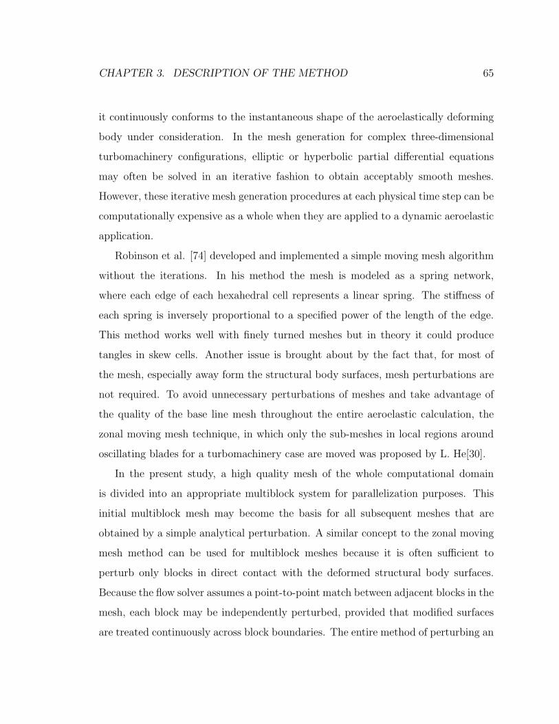
CHAPTER 3. DESCRIPTION OF THE METHOD 65
it continuously conforms to the instantaneous shape of the aeroelastically deforming
body under consideration. In the mesh generation for complex three-dimensional
turbomachinery configurations, elliptic or hyperbolic partial differential equations
may often be solved in an iterative fashion to obtain acceptably smooth meshes.
However, these iterative mesh generation procedures at each physical time step can be
computationally expensive as a whole when they are applied to a dynamic aeroelastic
application.
Robinson et al. [74] developed and implemented a simple moving mesh algorithm
without the iterations. In his method the mesh is modeled as a spring network,
where each edge of each hexahedral cell represents a linear spring. The stiffness of
each spring is inversely proportional to a specified power of the length of the edge.
This method works well with finely turned meshes but in theory it could produce
tangles in skew cells. Another issue is brought about by the fact that, for most of
the mesh, especially away form the structural body surfaces, mesh perturbations are
not required. To avoid unnecessary perturbations of meshes and take advantage of
the quality of the base line mesh throughout the entire aeroelastic calculation, the
zonal moving mesh technique, in which only the sub-meshes in local regions around
oscillating blades for a turbomachinery case are moved was proposed by L. He[30].
In the present study, a high quality mesh of the whole computational domain
is divided into an appropriate multiblock system for parallelization purposes. This
initial multiblock mesh may become the basis for all subsequent meshes that are
obtained by a simple analytical perturbation. A similar concept to the zonal moving
mesh method can be used for multiblock meshes because it is often sufficient to
perturb only blocks in direct contact with the deformed structural body surfaces.
Because the flow solver assumes a point-to-point match between adjacent blocks in the
mesh, each block may be independently perturbed, provided that modified surfaces
are treated continuously across block boundaries. The entire method of perturbing an
CHAPTER 3. DESCRIPTION OF THE METHOD 66
SURFACEPERTURBATION
ELASTIC
FACE ANDINTERIOR MESHPERTURBATION
EDGE AND SURFACEPERTURBATION
Figure 3.6: Moving Mesh Procedure
existing multiblock mesh to create a new one for the next time step takes a four-stage
procedure as shown in Figure 3.6. First, all block faces that are directly affected
by the structural motion of the body are explicitly perturbed by the deformation
tracking algorithm described in Section 3.3.1. Secondly, all edges that are in contact
with a face of the structural body, either in the same or in an adjacent block, are
implicitly perturbed with the algebraic method described below. Next, all faces that
either include an implicitly perturbed edge or adjacent to a structural body face are
implicitly perturbed with an algebraic method for each index line. Finally, the interior
points belong to all blocks that have one or more explicitly or implicitly perturbed
faces are perturbed in the same way as the edge and face perturbations.
For edge, face and block perturbation in these procedures, the arc-length attenua-
tion algorithm developed by Reuther et. al. [75] is used because it is mathematically
very simple but can avoid tangles of the meshes and maintain high mesh quality. In
this algorithm, all the original mesh points are first transfered to another coordinate

CHAPTER 3. DESCRIPTION OF THE METHOD 67
system where each component is related to its arc length along the index line that
the mesh point lies, and then normalized with the total arc length of that index line.
Once both ends of the index line are perturbed, then all the mesh points in between
are moved by an amount which is attenuated by the arc length, thus always main-
taining their transfered normalized coordinates. According to the entire procedure
described above, the second stage shifts the eight corner points of the block in ques-
tion and corrects the perturbations of the twelve edges of the block resulting from the
corner shifts to attain the final desired edge locations. The third stage corrects the
perturbations of the six faces surrounded by these edges. Finally, the fourth stage
corrects the interior points to produce the desired new mesh with face point motions
accounted for.
As far as the geometric conservation law is concerned, this moving mesh procedure
combined with the dual time stepping keeps the same order of accuracy in time as
the time derivative operator described in Section 3.1.3. The geometric conservation
law given in Equation 2.42 can be applied to each cell of the computational domain.
Although the boundary velocity of a cell on the structural surface can be transfered
from the node velocities of the structural model by the deformation tracking system
in Section 3.3.1, the determination of the boundary velocity of an interior cell needs
to rely on the discretization of the grid positions in time using the time derivative
operator. Thus, the left hand side of Equation 2.42 results in an approximation with
the same order of accuracy in time as the time derivative operator. In fact, this
approach, however, does not affect the accuracy of the unsteady computation. As
discussed later, the accuracy in time of the coupled system is as high as first order
which would be less than the accuracy of the geometric conservation law if the second
or third order derivative was used.
Although this mesh perturbation algorithm for multiblock meshes is quite sophis-
ticated for most external flow applications, it is not inevitable that the method might

CHAPTER 3. DESCRIPTION OF THE METHOD 68
produce poor mesh qualities when large perturbations happen within a small block.
In turbomachinery, any mesh topology for a multiblock system is forced to have at
least one block which represents the tip clearance region. This block usually has the
stationary casing surface on one face and the tip section of the blade or an implicitly
perturbed face by the motion of the tip on the opposite face. Furthermore the length
of this kind of block in the radial direction is very short but the deflections at the tip
of the perturbed faces in the circumferential direction is fairly large. As a result, the
short edges in the radial direction will become oblique as illustrated in Figure 3.7.
This poor quality of the mesh in the tip clearance region may fatally affect accuracy
and stability of the computation because the flow complexity around this region is
severe due to the transonic flow and vortex shedding at the tip.
To overcome this difficulty, another mesh perturbation procedure for this partic-
ular region must be introduced. Instead of keeping the mesh points on the casing
stationary, they are allowed to slide along the casing surface such that the blocks
representing the tip clearance maintain their mesh quality as much as possible. The
arc-length attenuation method is also used in this process. The procedure taken in
this study is as follows. First, the faces on the blade or the implicitly perturbed faces
are perturbed according to the aeroelastic motion of the blade. Second, the leading
edge and the trailing edge of the tip section are extended along each edge line in the
span-wise direction to the casing in order to detect the crossing point on the casing
using some interpolations. Once the corner points of the block on the casing are
determined, the next step is to move the edges, faces, and interior points of the block
for the tip clearance region according to the arc-length attenuation method. Note
that when the edges and faces on the casing are perturbed, the points on the casing
are forced to lie along the original casing surfaces using interpolations.
Figures 3.8 and 3.9 show how a block surface is perturbed using the usual block
perturbation and the improved procedure for the tip clearance, respectively. The

CHAPTER 3. DESCRIPTION OF THE METHOD 69
Casing
Hub
Blade
Tip Clearance
Before Perturbation
Improved ProcedureUsual Procedure
After Perturbation
Figure 3.7: Moving Mesh Procedure in the Tip Clearance Region
figures show the view of the trailing edge at the tip of the blade looking inward
radially from the casing. The meshed and solid surfaces in the figures represent the
original and new location of the blade, respectively. Without the improved procedure,
the block for the tip clearance is sheared by the tip motion of the blade and the
stationary casing resulting in the poor quality of the interior cells. On the other hand,
the improved procedure creates the new mesh as if the blade were extended through
the casing such that the original mesh quality of the block for the tip clearance can
be maintained.

CHAPTER 3. DESCRIPTION OF THE METHOD 70
Figure 3.8: Perturbed Mesh for the Tip Clearance Using the Usual Procedure
Figure 3.9: Perturbed Mesh for the Tip Clearance Using the Improved Procedure

CHAPTER 3. DESCRIPTION OF THE METHOD 71
3.2 Structural Mechanics
In the classical linear theory for aeroelastic problems, the structural model can be
reduced to a small degree of freedom eigenvalue problem to solve for the amplitude
of each degree of freedom. The earliest structural model was probably the Typical
Section [47] with two degrees of freedom, plunging and pitching motions of each blade.
However, if a nonlinear aerodynamic model is used, it is generally more efficient to
perform aeroelastic analysis in the time domain, by integrating the fluid/structure
coupled equations providing more accurate structural responses.
For an independent structural analysis of turbomachinery blades, researchers tra-
ditionally have modeled blades as one-dimensional straight, slender, twisted, elastic
beams, with symmetric varying cross sections, based on a continuum beam method
such as the Rayleigh-Ritz method. However, when the blade span is small and suf-
ficiently wide along its chord, it behaves more like a plate or shell rather than a
beam. The classical beam theory is not valid anymore as it cannot predict plate
modes. Modern fan and compressor blades are thin and have a considerable amount
of built-in pre-twist especially for fan blades. In addition, rotor blades are inertially
coupled by operation in a strong rotational body force field. The flat-plate theory
[76] and the thin shell theory with camber, twist and rotation [77] have proven useful
with the Rayleigh-Ritz method in determining the mode characteristics of blades.
While energy methods such as the Rayleigh-Ritz method require a lot of analytical
background work, a finite element model is relatively simple but able to represent
more complex blade structure accurately. As far as the interaction between the fluid
system and the structural system is concerned, a finite element model is more con-
venient because the local displacements and loads can be represented at adequately
distributed nodes which can simply communicate variables with the close mesh points

CHAPTER 3. DESCRIPTION OF THE METHOD 72
in the fluid system. In this study, an industry standard finite element analysis pack-
age, MCS/NASTRAN, is used for its reputation in capability and accuracy and its
large library of elements.
Some researchers also addressed the importance of modeling the rotor structure
as a bladed-disk assembly [78]. The bladed-disk assembly exhibits the same vibration
properties as a simple disk, but the relative disk and blade flexibilities determine
the overall characteristics of the vibration. For long-span wide-chord fans, the disk
is usually much stiffer than the blade, hence assembly modes are dominated by the
blade characteristics [79]. Since such fans are the main interest in this study because
they are the most critical in terms of flutter boundaries, rotor disks are not included
in the structural modeling. Modeling a bladed-disk assembly would be more realistic
but it would require flow calculations with the whole wheel of the rotor, which would
be computational quite expensive and not expected to give more accuracy.
In this section, fundamentals of the finite element analysis are discussed followed
by discussions on the modeling of turbomachinery blades especially about the choice
of the finite element, damping characteristics and the inclusion of centrifugal and
Coriolis forces. Finally a numerical method for integrating the structural equation in
time to calculate nodal displacements at each period is discussed.
3.2.1 Finite Element Analysis
In structural finite element analysis [80, 81], a body is approximated as an assembly
of discrete finite elements interconnected at nodal points on the element boundaries.
The material displacement measured in a local coordinate system (x, y, z), within
each element is assumed to be a function of the displacements at nodes of the finite
element. For element m, the displacements u(m) at a point in space (x, y, z) is written
as,
CHAPTER 3. DESCRIPTION OF THE METHOD 73
u(m)(x, y, z) = H (m)(x, y, z)q, (3.42)
where H(m) is the displacement interpolation matrix, the superscript m denotes ele-
ment number m, and q is the vector of the six global displacements at all the nodal
points of element m. The six components basically include translational components
in the three Cartesian directions and rotation components about the same axes if
elements with rotational degrees of freedom are considered. The entries in H(m)
depend on the element geometry, the number of element nodes and degrees of free-
dom, and the element parameterization chosen. This relation is appropriate for small
displacements of the structure but may lead to severe grid distortions when the struc-
ture undergoes large deflections. With the assumption that the displacements can be
represented by Equation 3.42, the corresponding strain can be evaluated using the
strain-displacement relations in Equations 2.30.
ε(m)(x, y, z) = B(m)(x, y, z)q, (3.43)
where B(m) is the strain-displacement matrix which is obtained by differentiating
H(m). Furthermore, the stresses in the finite element are related to the element
strain by the strain-stress relations in Equations 2.31.
σ(m) = C(m)ε(m), (3.44)
where C(m) is the elasticity matrix of element m and its components are given in
Equations 2.31. The material property specified in C(m) for each element can be
assumed to be that for an isotropic material and to depend on the type of the element.
Using these assumptions, the principle of virtual work in Equations 2.35 for the
assembly of finite elements is now considered and rewritten as a sum of integrations
over the volume and area occupied by all finite elements,

CHAPTER 3. DESCRIPTION OF THE METHOD 74
∑m
∫
V (m)
δε(m)T σ(m)dV (m) =∑m
∫
V (m)
δu(m)T[−ρ(m)u(m) − κ(m)u(m)
]dV (m)
+ δqT · f ,
(3.45)
where f is a global vector of concentrated loads applied to the finite element assembly.
Notice that the ith component in f is the concentrated nodal force that corresponds
to the ith displacement component in q. The last term in this equation, the work
done by the aerodynamic force, is computed using the conservation of energy principle
discussed in Section 2.3.1. These loads must also be equivalently transfered from the
external aerodynamic forces applied to the structure according to the conservation of
loads. The method of transformation is discussed in Section 3.3.2. Substitution of
3.42, 3.43 and 3.44 into Equation 3.45 yields,
[M ]q+ [C]q+ [K]q = f, (3.46)
where
[M ] =∑m
∫
V (m)
ρ(m)H(m)T H(m)dV (m),
[C] =∑m
∫
V (m)
κ(m)H(m)T H(m)dV (m),
[K] =∑m
∫
V (m)
B(m)T C(m)B(m)dV (m). (3.47)
[M ], [C] and [K] are the mass, damping and stiffness matrices, respectively. In
practice it is difficult, if not impossible, to determine the element damping parameters
in [C] for general finite element assemblies . The damping characteristics of the
structure are discussed in Section 3.2.3 in more detail.
In a time-marching aeroelastic analysis, once the matrices [M ], [C], [K] and the

CHAPTER 3. DESCRIPTION OF THE METHOD 75
load vector f are calculated, the equations of motion 3.46 can be integrated in
time starting from initial conditions for the vectors q and q. Thus the structural
response given by the time history of the displacement vector q can be obtained.
MSC/NASTRAN offers two types of solution sequences for transient response
analysis with time-dependent loads; the direct linear transient solution sequence
(SOL109), and the direct nonlinear transient response solution sequence (SOL129).
Since the aerodynamic loads acting on the blade are updated during the aeroelas-
tic computation sequence and cannot be formulated as an explicit function of time,
MSC/NASTRAN solves the structural response at each physical time step assuming
constant loads during the period that starts with the initial conditions given by the
solutions for the previous time step. SOL109 is typically used for models built with
linear elements, but it cannot specify both initial displacements and velocities. Al-
though the structural models used in this study are all built with linear elements,
SOL109 is not properly suited for this particular application. Therefore SOL129 is
used, because it can handle any initial condition as well as linear elements [82].
3.2.2 Finite Element Model
The finite element method offers many options for the structural dynamic analysis
of swept and twisted blades. From these available options, plate or shell elements of
rectangular or triangular shapes are commonly used since fan blades are quite thin
[83]. In MSC/NASTRAN, several elements are available for shell structures. They can
be both flat triangles (TRIA3, TRIA6), or flat rectangles (QUAD4, QUAD8). TRIA6
and QUAD8 are higher order elements that have quadratic interpolation functions;
the displacements at any point in an element are assumed to be specified as quadratic
functions of the nodal displacements. Meshes with higher order elements can, in
theory, provide the same quality of results as meshes with with larger number of
lower elements. However, any inherent error found in calculated results on a mesh

CHAPTER 3. DESCRIPTION OF THE METHOD 76
consisting of lower order finite elements vanishes as the mesh is refined. From a
practical standpoint, the blade, even if modeled with a relatively coarse lower order
mesh should not result in large deviations from the exact solution. In this study, a
simplified blade model that consists of varying-thickness linear shell elements is used.
TRIA3 and QUAD4 are the three-node and four-node triangular and quadrilateral
linear finite elements provided by MCS/NASTRAN. These elements have six degrees
of freedom per node, i.e., two membrane displacements, one membrane rotation, one
bending displacement and two bending rotations. These six degrees of freedom can
be easily converted into three translations and three rotations along and about the
axes of a Cartesian coordinate system fixed in space. The element thickness is al-
lowed to vary over the element surface. Lumped and consistent mass formulations
are considered. As discussed later in Section 3.3, each fluid mesh point on the blade
surface is associated with a projected point on the closest structural element surface
for purpose of information exchange between the fluid and structural systems. Ob-
viously, the search for projected points on a flat surface is much simpler than if the
surface were curved. While the four nodes of a quadrilateral element do not always lie
on a plane, the nodes of a triangular element always do independently of the element
interpolation function. In this study, TRIA3 has been used because of its sufficient
accuracy for the this type of fluid-structure interface.
3.2.3 Damping Characteristics
For turbomachinery blades, damping may be arising from aerodynamic forces, vis-
cous damping, and material hysteresis [84]. For most blades the primary source of
damping is aerodynamic damping due to the time-dependent aerodynamic loading
generated by the blade motion. In an aeroelastic computation, the aerodynamic
damping is calculated by the flow solver and is not included in the structural model.
It depends on the rotation speed, pressure ratio, inter-blade phase angle, or any other

CHAPTER 3. DESCRIPTION OF THE METHOD 77
factor that can affect the flow field. Unlike aerodynamic damping, the viscous and
material damping characteristics are essentially determined by how the structure is
built. Viscous damping gives rise to a force which opposes the motion proportionally
to its velocity. It is mainly due to mechanical friction observed at the blade attach-
ment to the disk or to the collision of the blade shrouds. It is considered to be very
difficult to model viscous damping in structural models, in particular because the
damping properties are usually frequency dependent. On the other hand, material
damping is related to the total energy loss of the motion by material hysteresis which
result in heat radiation. Although material damping is proportional to the square of
frequency, this internal material damping is negligible even for the higher frequency
modes, especially when the blade is made of a stiff material such as titanium. In this
study, only viscous damping is included in the structural model for these reasons.
The viscous damping force is usually modeled as a function of a damping coefficient
and the velocity of the structural body motion. It is represented in the equation of
motion 3.46 using the damping matrix [C] and the velocity vector. Unlike mass and
stiffness properties, damping properties are not easy to model in a general fashion.
For this reason, damping models tend to be application specific. For instance, when
the structural equations are reduced to the superposition of several dominant modes,
the viscous damping coefficient is independently specified in the equation of motion
for each mode. In usual aeroelastic analysis using finite element methods, the viscous
damping is set to zero as its effects can be added later in a linear fashion. For
example, the damping matrix [C] is explicitly constructed by assuming that it is a
linear function of the mass matrix [M ] and the stiffness matrix [K] of the complete
element assembly, together with experimental results. For turbomachinery blades, it
is more realistic to include the viscous damping by means of a stiffness proportional
damping rather than a mass proportional damping.

CHAPTER 3. DESCRIPTION OF THE METHOD 78
Incidentally, the material damping force depends on the displacements. It is ex-
pressed as a function of a damping coefficient and a complex component of the struc-
tural stiffness matrix. In practice, if the viscous damping force is assumed to be
proportional to the stiffness force, it can be expressed by the same function. Let G
denote the viscous damping coefficient, then Equation 3.46 can be rewritten as
[M ]q+ 1 + iG[K]q = f. (3.48)
Consider the oscillatory response for a single degree of freedom system, mq+cq+kq =
f , where m, c, k, q and f are the mass, the viscous damping coefficient, the stiffness
coefficient, the displacement and the applied force, respectively. The solution of
the equation of motion yields terms of type q = q0e−ζωt which ensure that the time
histories will decay for positive damping coefficients. The damping forces in Equation
3.48 and in the single degree of freedom system are identical if
kG = cω. (3.49)
Therefore, if G is to be modeled using an equivalent viscous damping c, then Equation
3.49 holds at only one frequency ω. Two parameters c and ω need to be specified
to convert the viscous damping to an equivalent stiffness proportional damping. In
this study, damping characteristics are modeled in this way choosing the first natural
frequency of the structural model for ω and assuming c.
3.2.4 Centrifugal and Coriolis Forces
In predicting the natural modes and frequencies of rotor blades, it is essential to take
into account the effect of the rotor rotational speed. The inertial forces due to the
rotation of a blade tend to stiffen the transverse bending elastic springs. In vibration
analysis, these forces approximately increase the square of the natural frequency ω2n

CHAPTER 3. DESCRIPTION OF THE METHOD 79
in proportion to the square of the rotation speed Ω2. This effect can be described
by stating ω2n = ω2
0n + κnΩ2 where ω0n is the non-rotating natural frequency of the
rotor blade and κn is a proportionality constant for the nth mode. The effect is most
notable in the natural modes which exhibit predominantly bending displacements,
usually the lowest frequency mode. Thus, for high-speed rotors, the inertial forces
may be of importance in the aeroelastic problem.
These forces appear in the equations of motion as three additional terms. Assume
that the rotating system spins about the x-axis with a constant frequency Ω relative
to the stationary system, then the equations of motion for a particle in the rotating
elastic structure with externally applied forces f can be written as,
[M ]q+ ([C]− Ω[Cc]) q+([K]− Ω2[Kc]
) q = f+ Ω2[Kc]q0, (3.50)
where q0 is the position vector of the particle in the stationary system and qis the displacement of the particle. The term Ω[Cc]q is commonly refered to as
the Coriolis force and the term Ω2[Kc](q0 + q) is refered to as the centrifugal
force. Notice that the centrifugal force term in the right hand side of the equation
behaves as a body force during the solution procedure. The matrices [Cc] and [Kc]
for a system rotating about the x-axis can be written as,
[Cc] =
0 0 0
0 0 −2m
0 2m 0
, [Kc] =
0 0 0
0 m 0
0 0 m
, (3.51)
where m is the mass of the particle. Notice that the centrifugal force is dependent
on the current position vector of the particle, and divided into two terms: the term
proportional to the stationary position vector and that proportional to the displace-
ment vector. While the stiffness and damping terms in Equation 3.50 for a rotating
CHAPTER 3. DESCRIPTION OF THE METHOD 80
system are the same as those in a stationary system, the part of the centrifugal term
proportional to the displacement behaves as an additional stiffness term because it
is proportional to the displacement. Similarly, the Coriolis term acts as additional
damping in the equation of motion. These two terms are refered to as gyroscopic
terms hereafter.
For the computation of frequencies and mode shapes using MSC/NASTRAN, it
is possible to include the gyroscopic terms described above by using two solution se-
quences [85]. First, the gyroscopic terms are calculated in a steady-state displacement
analysis run using solution sequence (SOL101) and the Direct Matrix Abstraction
Program (DMAP) [86] included with the SSSAlter Library “segyroa.v705” [82]. The
centrifugal force field in the right hand side of Equation 3.50 is computed by using
the blade’s stational geometry, mass properties and the rotational speed specified in
the “RFORCE” card in the input file. This solution sequence computes steady-state
displacements and then stores the blade modified stiffness and mass matrices in a
database. Then, the gyroscopic terms are added to the global stiffness and damping
matrices for the translational degree of freedoms in the direction of two axes perpen-
dicular to the axis of rotation. Following SOL101, an eigenanalysis solution sequence
(SOL103) is run to yield natural frequencies and mode shapes. Unfortunately, the
current version of MCS/NASTRAN does not have the capability to include the gy-
roscopic terms in the direct transient response solution sequences which are required
for solving the structural response of the blade with time-dependent nonlinear aero-
dynamic loads with initial conditions provided by the displacements and velocities of
the last transient solution sequence.
Alternate approach taken in this study is to adjust the material properties of the
rotating structure to create a stiffness model which accounts for gyroscopic effects.
The gyroscopic effects are known to be significant on the first mode but are hardly
recognizable on higher frequency modes for typical turbomachinery rotor blades [83].

CHAPTER 3. DESCRIPTION OF THE METHOD 81
An increase of the stiffness by changing material parameters such as Young’s modulus,
density and the thickness of the linear elements usually shifts all natural frequencies
higher resulting in too high frequencies for higher frequency modes. However, the
frequencies of higher frequency modes are not considered to influence the stability
of the blade motions because flutter in turbomachinery is single degree of freedom
instability as discussed in Chapter 1. Thus it is considered to be sufficient to model
the structure with a realistic lowest frequency for observing the aeroelastic behavior
of the blade in a flutter condition.
3.2.5 Time Integration
Efficient and accurate numerical integration schemes for a second order system, such
as Equation 3.46, have been proposed by many researchers [80]. Houbolt presented
an implicit, three-step recurrence scheme. The most popular Newmark method pro-
vides a single-step family of methods employing two integration parameters (βN , γN)
to give a variety average approximation of the acceleration term. Wilson introduced
a family of implicit methods employing a single integration parameter. Katona and
Zienkiewicz [87] introduced a generalization of Newmark’s time marching integra-
tion scheme, called beta-m method, in which the most well-known methods (e.g.
Newmark, Wilson, Houbolt, etc.) are shown to be special cases within the beta-m
family. In the present work, the equations of structural motion are advanced in time
by using a modified Newmark method, which is unconditionally stable, included in
MSC/NASTRAN [88].
When the displacements are solved for at discrete times, typically a fixed integra-
tion time step ∆t is used. A central finite difference representation of the velocity
q and acceleration q vectors at discrete times becomes,

CHAPTER 3. DESCRIPTION OF THE METHOD 82
qn =1
2∆t
(qn+1 − qn−1),
qn =1
∆t2(qn+1 − 2qn+ qn−1
). (3.52)
Averaging the displacement and the applied force over three adjacent time steps, the
structural equations of motion 3.46 can be rewritten as,
[M
∆t2
] (qn+1 − 2qn+ qn−1)
+
[C
2∆t
] (qn+1 − qn−1)
+
[K
3
] (qn+1+ qn+ qn−1)
=1
3
(fn+1+ fn+ fn−1).
(3.53)
Rearranging the equation, it becomes
[A1]qn+1 = f 1+ [A2]qn+ [A3]qn−1, (3.54)
where,
[A1] =
[M
∆t2+
1
2∆tC +
K
3
],
[A2] =
[2M
∆t2− K
3
],
[A3] =
[− M
∆t2+
C
2∆t− K
3
],
f 1 =1
3
(fn+1+ fn+ fn−1). (3.55)
This approach is similar to the classical Newmark direct integration method except
that f is averaged over three time points. The transient solution is obtained as a series
of static solutions at each time step by factoring [A1] and applying it to the right-
hand side of the above equation which consists of all the known variables. Assuming

CHAPTER 3. DESCRIPTION OF THE METHOD 83
that, the [M ], [C], and [K] matrices are constant throughout the analysis and do
not change with time, the factorization of [A1] can be stored and does not need to
be recomputed if the time step, ∆t, is constant. Under similar considerations, [A2]
and [A3] also remain constant throughout the analysis. The transient nature of the
solution is carried through by modifying the applied force vector, f 1.
3.3 Fluid-Structure Interface
As discussed at the beginning of this chapter, the flow and structural solvers used in
this study have been independently developed and an appropriate interface needs to
be developed to couple the two solvers. In early fluid/structure coupled aeroelastic
calculations for external flows, the same surface discretization for the fluid and struc-
tural domains with the same size of the surface elements was used to transfer loads
and deformations between the two disciplines without the need for any interpolations
[89]. The same assumption was made for turbomachinery flow by Imregun and his
collaborators [52, 53]. The fluid system and the structural systems, however, essen-
tially use different surface discretizations because of differing accuracy requirements
in the resolution of the features of each solution. The fluid system usually requires
a finer mesh to capture nonlinear features such as shock waves and boundary layers.
Moreover, the type of element that each solver uses might also cause mismatches of
the mesh points on the interface. In this study, while the flow solver employs rel-
atively finer multiblock structured meshes, the structural solver employs triangular
elements. This mismatch of mesh points on the interface gives rise to the necessity of
a numerical approximation to transfer the pressure distribution on the fluid surface
mesh to a corresponding nodal load distribution on the structure and also for the
transfer of the displacements of the structural nodes to corresponding perturbations
of the fluid mesh.

CHAPTER 3. DESCRIPTION OF THE METHOD 84
The level of the accuracy in the coupling process must be carefully considered so
as not to forego solution quality sought by the high accuracy in the discretization
of the individual disciplines. One of the principles that is needed to support the
maintenance of coupling accuracy is the conservation of loads and energy given in
Section 2.3.1 which states that the sum of the nodal forces in the structural system
transfered from the pressure field in the fluid system must be equal to the integral of
the pressure fields on the body surface boundary in the fluid system. In this study,
the approach formulated from the conservation of loads and energy by Brown [90],
and later followed by Reuther et al [91] in aero-structural optimization, is chosen to
ensure that the transfer of the pressure fields to the nodal forces is both consistent
and conservative. Brown’s approach can also be used in the extrapolation of the
nodal displacement in the structural system to the mesh deformation on the surface
of the fluid system.
In addition, the fluid system usually requires a finer temporal resolution than
the structural vibration for most aeroelastic problems. In computations, while the
flow solver employs the Runge-Kutta time integration which has a stability limit, the
structural solver uses the Newmark time integration which is unconditionally stable.
This difference in the stability limits need to be taken care of by a synchronization
approach between the two solvers alternatively advancing in time with different time
steps.
In the following sections, the detail descriptions are given for the individual inter-
face algorithm starting from the deformation tracking system, followed by the load
transfer system and the synchronization.
3.3.1 Deformation Tracking System
In most cases of aeroelastic analysis of turbomachinery, the blade may be simply
modeled with shell elements which usually have fewer nodal points than the outer
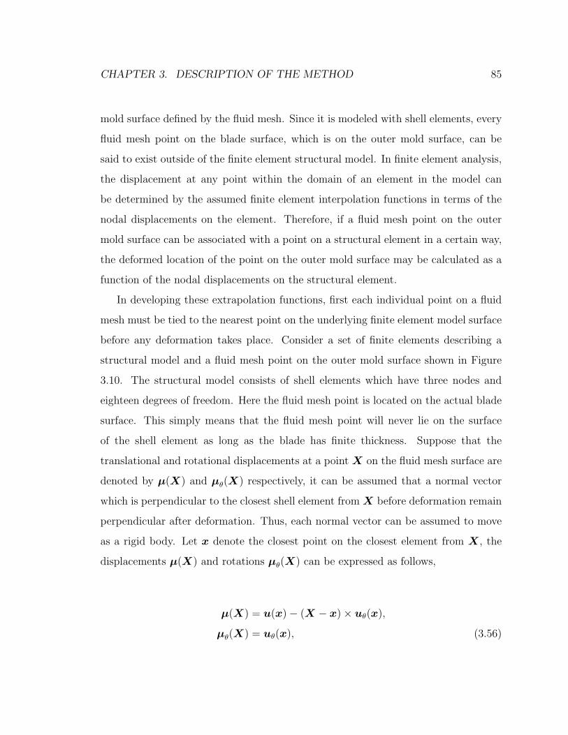
CHAPTER 3. DESCRIPTION OF THE METHOD 85
mold surface defined by the fluid mesh. Since it is modeled with shell elements, every
fluid mesh point on the blade surface, which is on the outer mold surface, can be
said to exist outside of the finite element structural model. In finite element analysis,
the displacement at any point within the domain of an element in the model can
be determined by the assumed finite element interpolation functions in terms of the
nodal displacements on the element. Therefore, if a fluid mesh point on the outer
mold surface can be associated with a point on a structural element in a certain way,
the deformed location of the point on the outer mold surface may be calculated as a
function of the nodal displacements on the structural element.
In developing these extrapolation functions, first each individual point on a fluid
mesh must be tied to the nearest point on the underlying finite element model surface
before any deformation takes place. Consider a set of finite elements describing a
structural model and a fluid mesh point on the outer mold surface shown in Figure
3.10. The structural model consists of shell elements which have three nodes and
eighteen degrees of freedom. Here the fluid mesh point is located on the actual blade
surface. This simply means that the fluid mesh point will never lie on the surface
of the shell element as long as the blade has finite thickness. Suppose that the
translational and rotational displacements at a point X on the fluid mesh surface are
denoted by µ(X) and µθ(X) respectively, it can be assumed that a normal vector
which is perpendicular to the closest shell element from X before deformation remain
perpendicular after deformation. Thus, each normal vector can be assumed to move
as a rigid body. Let x denote the closest point on the closest element from X, the
displacements µ(X) and rotations µθ(X) can be expressed as follows,
µ(X) = u(x)− (X − x)× uθ(x),
µθ(X) = uθ(x), (3.56)

CHAPTER 3. DESCRIPTION OF THE METHOD 86
µ (X)CFD Mesh Point DEFORM
u(x)
q , q , q1 2 3
q , q , q
q , q , q
1 2 3
7 8 9
13 14 15
Finite Elemet
A
A
A
1
2
3
Figure 3.10: Deformation Tracking System
where u(x) and uθ(x) are the displacement and rotation at x. Given a set of values
for the eighteen nodal displacements, displacements and rotations at any point on a
triangle shell element can be evaluated using the original finite element interpolation
functions. However, since MSC/NASTRAN is used as a structural solver and the
finite element interpolation function used in it is unknown, all of the finite elements
were assumed to use the simple standard iso-parametric interpolation function based
on the area coordinate as the weighting. When the fluid mesh point X is associated
with x on the mth element whose displacements are denoted as q(m), this interpolation
function can be expressed as,
u(x) =[η(m)(x)
] · q(m) =[[A
(m)1 ][0][A
(m)2 ][0][A
(m)3 ][0]
]· q(m),
uθ(x) =[η
(m)θ (x)
]· q(m) =
[[0][A
(m)1 ][0][A
(m)2 ][0][A
(m)3 ]
]· q(m), (3.57)
where [0] is the 3×3 zero matrix and [A(m)1 ], [A
(m)2 ] and [A
(m)3 ] are defined by the area
CHAPTER 3. DESCRIPTION OF THE METHOD 87
coordinates [80]. For example, [A(m)1 ] is expressed using the area coordinate shown in
Figure 3.10 as follows,
[A(m)1 ] =
A1 0 0
0 A1 0
0 0 A1
. (3.58)
The displacements and rotations at any point on the fluid mesh surface can thus be
written in terms of the associated nodal displacements q(m) using Equation 3.57.
µ(X) =[η(m)(x)
] · q(m) − [X − x] ·[η
(m)θ (xn)
]· q(m),
µθ(X) =[η
(m)θ (x)
]· q(m), (3.59)
where, the matrix [X − x] in cross product form can be given by,
[X − x] =
0 (z − Z) (Y − y)
(Z − z) 0 (x−X)
(y − Y ) (X − x) 0
. (3.60)
Since the rotations of the fluid mesh points are not used in the actual computations
for the flow filed, only µ(X) needs to be calculated. Introducing the displacement
extrapolation functions N(X) based on the global nodal displacements q of the struc-
tural model, Equation 3.59 can be rewritten using q because q(m) is a part of q.
µ(X) = [N(X)] · q, (3.61)
where,
[N(X)] = [η(x)]− [X − x] · [ηθ(x)] . (3.62)
As the interpolation functions η(x) and ηθ(x) linearly evaluate the displacements

CHAPTER 3. DESCRIPTION OF THE METHOD 88
within the element, N(X) can be used to extrapolate the displacements linearly to
the point outside of the element. As long as the displacements are small enough
for the structure to be modeled with linear elements, these extrapolation functions
are accurate, and the simplest method satisfying a condition that the displacements
µ(X) must be continuous in the region of fluid mesh. The procedure to obtain these
interpolation functions N(X) is implemented in a preprocessing program followed
by the main solver. N(X) is thus precomputed and stored for later use during the
aeroelastic procedure and plays an important role in the load transfer algorithm as
discussed in the next section.
The computational approach for mesh perturbation described in Section 3.1.8 will
then move the mesh point in the whole fluid computational domain according to the
explicit perturbation of the fluid mesh points on the fluid/structure interface. In
the dual time stepping scheme, mesh velocities are necessary as well as the mesh
position. To obtain the mesh velocities, a backward difference is used with the old
mesh positions which are stored in the memory. No extrapolation from the nodal
velocity of the structural model is used even on the interface.
3.3.2 Load Transfer System
In this section, a method that transfers aerodynamic loads obtained through a stress
integration over the structural surface area in the fluid system to applied nodal forces
with which the structural equations of motion must be solved is described. In general,
aerodynamic forces that act on a structural surface are divided into two categories
except for the body forces already ignored in the fluid equations. One is pressure
forces pushing the surface perpendicularly to the surface, the other is viscous shear
forces which appear when viscous calculations are performed in the fluid system.
Since the magnitude of shear forces is trivial compared to that of pressure forces,
viscous shear forces are not transfered from the fluid system to the structural system

CHAPTER 3. DESCRIPTION OF THE METHOD 89
in this study.
For a load transfer algorithm, it is required to satisfy the conservation of load
and energy expressed in Equations 2.36 and 2.37, respectively. In Equation 2.37,
δµ(X) can be related with δq introducing a set of assumed displacement interpolation
functions N(X) given in Equation 3.61. Substituting Equation 3.61 into Equation
2.37 yields,
f · δq =
∫
∂Ω
p · [N(X)] δqdS, (3.63)
where f is the global nodal force vector for the structural model. In practice, the
fluid pressure is taken as constant over a face around a fluid mesh point. Consider
the complementary projected surface area vector Si around the fluid mesh point
X i surrounded by the corner points which are given by simply averaging the corner
points of each face of the fluid mesh as shown in Figure 3.11, the right hand side of
the Equation 3.63 can be discretized as follows,
f · δq =∑
i
piSi · [N(X i)] δq. (3.64)
This allows the fluid pressure within each face to be taken out of the summation,
f i = piSi [N(X i)] , (3.65)
where f i is the nodal force vector given by the contribution of the pressure at the
fluid mesh point X i, which components are shown in Figure 3.11. The nodal force
vector for the m-th element denoted by f (m) is now obtained by simply summing the
all f i whose fluid mesh point is associated with the m-th element.
At this point, the algorithm ensures that it satisfies the conservation of energy on
which the algorithm is based. The next question is whether it satisfies the conservation
of loads given in Equation 2.36. Since the interpolation function [N(X i)] consists of
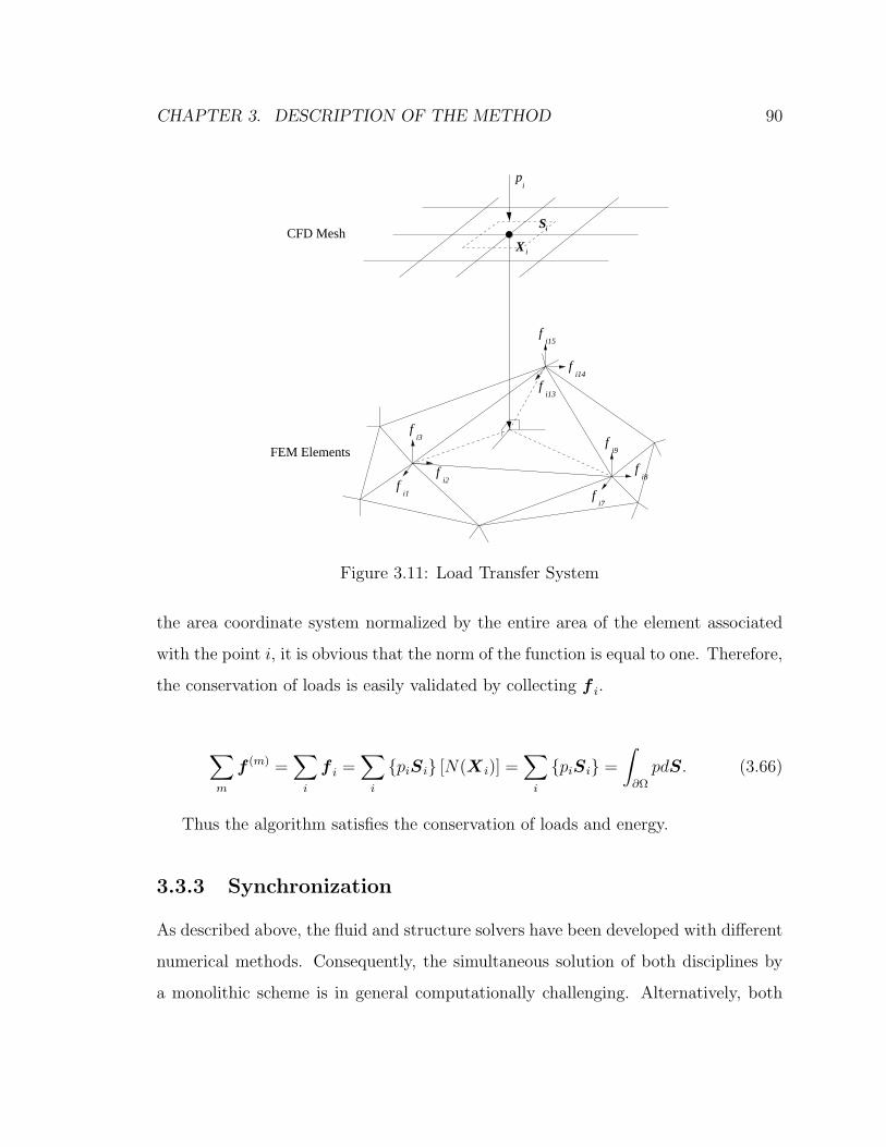
CHAPTER 3. DESCRIPTION OF THE METHOD 90
fi1
fi2
fi3
fi7
fi8
fi9
fi13
fi14
fi15
i
i
X i
CFD Mesh
FEM Elements
p
S
Figure 3.11: Load Transfer System
the area coordinate system normalized by the entire area of the element associated
with the point i, it is obvious that the norm of the function is equal to one. Therefore,
the conservation of loads is easily validated by collecting f i.
∑m
f (m) =∑
i
f i =∑
i
piSi [N(X i)] =∑
i
piSi =
∫
∂Ω
pdS. (3.66)
Thus the algorithm satisfies the conservation of loads and energy.
3.3.3 Synchronization
As described above, the fluid and structure solvers have been developed with different
numerical methods. Consequently, the simultaneous solution of both disciplines by
a monolithic scheme is in general computationally challenging. Alternatively, both

CHAPTER 3. DESCRIPTION OF THE METHOD 91
calculations are performed separately and synchronized. In many aeroelastic calcula-
tions, a steady flow is first computed around a structure in equilibrium or in a given
stationary condition with a set of initial displacements. Next the structure is allowed
to respond to the aerodynamic forces determined by the steady flow field. This should
be followed by a simple and popular staggered procedure as described below.
(1) Transfer the motion of the boundary of the structure to the fluid system using
the Deformation Tracking System and update the fluid mesh accordingly. At this
time, the updated cell volumes, projected areas and surface normals of all the cell
faces are calculated.
(2) Advance the fluid system W n+1 to a steady-state in pseudo-time and obtain
new pressure fields using the solutions at the time levels n, n− 1, and n− 2 stored in
memory for the third order accurate backward time discretization. An initial guess
for the solution at time level n + 1 is made equal to the solution at the previous time
level.
(3) Convert the new pressure fields into a set of nodal forces for the structural
model using the Load Transfer System.
(4) Advance the structural system under the given set of nodal forces.
The procedure repeats from step (1) through (4) until the desired time-marching
solutions are obtained. The basic staggered algorithm outlined above is graphically
illustrated in the left diagram of Figure 3.12 where W denotes the flow variables, q de-
notes the structural displacements, and p denotes the fluid pressure. The superscript
n designates the n-th time-station. The simplicity of this procedure is attractive and
apparently has earned the highest popularity among synchronization procedures for
aeroelastic computations in the time domain.
In most of the aeroelastic problems, different time scales are chosen for the fluid
and structure systems. The fluid system usually requires a finer time resolution than
the structural system. For the flow solver, an explicit scheme such as Runge-Kutta

CHAPTER 3. DESCRIPTION OF THE METHOD 92
1
2
4
3
W W
q
q
p
Fluid
Structure
n n+1
nn+1
n+11
2
4
3
W W
q
q
p
Fluid
Structure
Dual Time Steppingn n+1
nn+1
n+1
Newmark Scheme
Figure 3.12: Simple Partitioned Stagger Procedures
scheme must be selected to integrate the semi-discrete equations in order to obtain
the time accurate solutions for each period. On the other hand, the implicit Newmark
trapezoidal rule, which is unconditionally stable, is usually selected to integrate the
equation of motion of the structure. If the procedure mentioned above is used to solve
the aeroelastic equations, the time step must be governed only by the critical time
step of the explicit fluid solver. It is also noted that since the fluid system must be
advanced in the physical time scale, the fast convergence methods such as the local
time stepping, or multigrid can not be available. Thus, using the same time step in
both fluid and structure system is not efficient in advancing the structural system.
This difference in allowable time step size is, however, overcome by the dual time
stepping scheme in which the fluid system is updated implicitly in physical time,
and the pseudo time step is introduced to integrate the fluid equations within the
physical time period as discussed in Section 3.1.3. In this way, the same physical
time step is used for both solvers [53], because the physical time step of the dual
time stepping in fluid calculation can be chosen arbitrary and the structural time
step has no limitation. Thus, the overall computational cost can be saved because
fewer computations are necessary for the structural solver and communication in
exchanging boundary information. The basic assumption for this method is that
during one time-step of the fluid, structural deflections are small, and that during

CHAPTER 3. DESCRIPTION OF THE METHOD 93
one time-step of the structure, the flow field (loads) remain approximately constant.
This procedure is also graphically illustrated in the right diagram of Figure 3.12.
As far as the accuracy in time is concerned, the dual time stepping scheme is
at least second-order accurate in time. The trapezoidal rule is also second-order
accurate. The resulting simple partitioned staggered procedure becomes first-order
accurate in time according to a simple Taylor expansion [62]. This particular choice of
the mixed time integration is motivated by the fact that the aeroelastic response of a
structure is often dominated by low frequency modes and therefore is most efficiently
predicted by an implicit time integration scheme.
3.4 Parallelization
A fluid/structure coupled time-marching computation is computationally very expen-
sive especially applied to a viscous flow. The cost may became particularly extrava-
gant when it is used to detect flutter boundaries for turbomachinery because many
cases may need to be performed changing conditions such as rotation speeds, pressure
ratios, and inter-blade phase angles. Parallel computing is one possibility to reduce
the computational cost for multidisciplinary computations so that these computations
could be of more practical use for the preliminary design process of turbomachinery.
As discussed in Section 3.3.3, the basic procedure for the coupling of the two disci-
plines is to advance both systems alternatively in time. Farhat [62, 92] also addressed
a possibility of advancing the fluid and structure equations in parallel. In this method,
the fluid and structure systems can run in parallel during the time interval indepen-
dently in different processors and exchange information on the interface at the end of
each period. However, the fluid solver usually requires much more computational cost
than the structure solver. As a result, the processors in charge of the structure part

CHAPTER 3. DESCRIPTION OF THE METHOD 94
may need to wait for a long time until the flow calculations are finished to be ready
to exchange information for the next time step. Given a number of processors, the
parallelization between the fluid and structure solvers might not help reduce the total
aeroelastic simulation time. Therefore, the parallelization strategies for this study
are considered independently on the fluid and structure solvers and more effort must
be made for the fluid solver than the structural solver.
For the flow solver, the multiblock method is conveniently used in the finite vol-
ume discretization of the flow filed over complex geometries. This method is based
on domain decomposition technique, with the flow domain being partitioned into a
number of sub-domains. Within each sub-domain, the flow equations are solved in
an independent manner, with the global nature of the flow being accounted for by
the periodic exchange of boundary information between neighboring blocks. This do-
main decomposition is designed not only for representing the complex geometry but
also helping a parallelization strategy [93]. The parallelization strategy adapted in
TFLO is based on this multiblock decomposition discussed in detail in this section.
This section also discussed on the parallelization of the structural solver which is very
simple and more intended for memory reduction rather than fast computation.
3.4.1 Flow Solver
In the multiblock strategy, the space in the computational domain surrounding a
geometry of interest is filled with a series of structured blocks of varying sizes. As
mentioned in Section 3.1.6, each block is surrounded by halo cells in which proper
boundary conditions are applied. The multiblock strategy makes use of these halo
cells to communicate with the neighboring blocks. By updating the flow variables in
the halo cells with those of the corresponding interior cells in the neighboring blocks,
the multiblock flow solver is allowed to proceed independently within each block
during each stage of the Runge-Kutta time integration procedure. This inter-block

CHAPTER 3. DESCRIPTION OF THE METHOD 95
communication for updating the variables in the halo cells is performed at the end of
each stage of the Runge-Kutta scheme at each level of the multigrid when the solver
calls the boundary conditions.
When the flow filed is partitioned into blocks and the number of processors used
for the computation is specified, the computational load for each processor can be
evenly distributed. According to the multiblock decomposition, the even distribution
of the computational loads is attempted by dividing the blocks into the same number
of groups as the number of processors used in the computation such that the differ-
ences among processors in terms of the amount of computation and communication
that they must perform is a minimum [93]. The number of blocks assigned to each
processor is not necessarily identical because the size of the block is usually not equal.
Typically, each processor is assigned a set of blocks of varying sizes but approximately
an equal total number of cells. In addition, the communication cost is also taken care
of by attempting to place blocks that share a physical interface on the same proces-
sors such that as much inter-block communication is processed within each processor
as possible to minimize the inter-block communication between different processors.
The data communication between fluid blocks assigned to different processors
is accomplished by using the Message Passage Interface (MPI) standard (www-
unix.mcs.anl.gov/mpi/index.html), which is a set of libraries for message passing
within a multi-processor computer. For example, MPI subroutines are called when
the solver applies boundary conditions at every stage of the Runge-Kutta time inte-
gration, or perturbs corner points and edges implicitly affected by the blade motion,
etc. Each processor individually proceeds to the computation of the next time step
as soon as its inter-block communication phase is completed not holding until all the
inter-block communications are done.
In the implementation of the parallelization scheme using the multiblock strategy,
a pre-processing module identifies the halo cells adjacent to the block boundaries and
CHAPTER 3. DESCRIPTION OF THE METHOD 96
constructs a list for each processor which contains the pointers for the halo cells in the
neighboring blocks and the corresponding processor number. The pre-processor also
calculates the computational and communication load for each block and performs
the load balancing for the parallel computation at the same time. Based on the
information on the list for each processors, the excursion of different programs onto
different processor are enabled by using an MPI command.
3.4.2 Structural Solver
MSC/NASTRAN has the capability of parallel processing in its package. This par-
allelization is intended to decompose the global matrices into smaller ones and solve
partitioned nodal displacements for a group of degree of freedoms in parallel, espe-
cially when the structure is modeled with a massive number of elements. However,
since the size of each blade structural model is not so large as to have a serious
influence on the aeroelastic computational cost, the parallelization strategy for the
structural solver used in this study should rather be directed at the multi-passage
computations in which multiple structural models of the blades need to be analyzed
at the same time. From the numerical experiment, MSC/NASTRAN can be executed
from different processors in a parallel computer with different input files at the same
time, and it yields the different results.
In multi-passage calculations, each blade has its own unique structural model.
The structural models are allocated in the processors so that the number of structural
models per processor is minimized. The number of structural models is usually less
than the number of blocks for the fluid calculations, and also less than the number
of processors used in the parallel computations. It is simply considered that some of
the processors possess the structural models, run the structural solver and distribute
the resulting solutions to the corresponding processors using MPI.
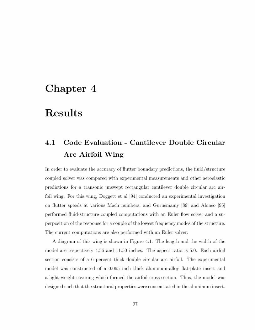
Chapter 4
Results
4.1 Code Evaluation - Cantilever Double Circular
Arc Airfoil Wing
In order to evaluate the accuracy of flutter boundary predictions, the fluid/structure
coupled solver was compared with experimental measurements and other aeroelastic
predictions for a transonic unswept rectangular cantilever double circular arc air-
foil wing. For this wing, Doggett et al [94] conducted an experimental investigation
on flutter speeds at various Mach numbers, and Gurusmamy [89] and Alonso [95]
performed fluid-structure coupled computations with an Euler flow solver and a su-
perposition of the response for a couple of the lowest frequency modes of the structure.
The current computations are also performed with an Euler solver.
A diagram of this wing is shown in Figure 4.1. The length and the width of the
model are respectively 4.56 and 11.50 inches. The aspect ratio is 5.0. Each airfoil
section consists of a 6 percent thick double circular arc airfoil. The experimental
model was constructed of a 0.065 inch thick aluminum-alloy flat-plate insert and
a light weight covering which formed the airfoil cross-section. Thus, the model was
designed such that the structural properties were concentrated in the aluminum insert.
97
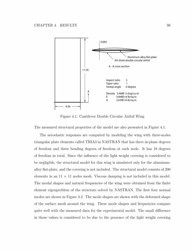
CHAPTER 4. RESULTS 98
11.50
A A
4.56
Aspect ratio 5 Taper ratio 1 Sweep angle 0 degree Density 3.468E-3 slug/cu-in E 9.848E+6 lb/sq-in G 3.639E+6 lb/sq-in
0.065
Aluminum alloy flat-plate6% think double circular airfoil
A - A cross section
Figure 4.1: Cantilever Double Circular Airfoil Wing
The measured structural properties of the model are also presented in Figure 4.1.
The aeroelastic responses are computed by modeling the wing with three-nodes
triangular plate elements called TRIA3 in NASTRAN that has three in-plane degrees
of freedom and three bending degrees of freedom at each node. It has 18 degrees
of freedom in total. Since the influence of the light weight covering is considered to
be negligible, the structural model for this wing is simulated only for the aluminum-
alloy flat-plate, and the covering is not included. The structural model consists of 200
elements in an 11 × 11 nodes mesh. Viscous damping is not included in this model.
The modal shapes and natural frequencies of the wing were obtained from the finite
element eigenproblem of the structure solved by NASTRAN. The first four normal
modes are shown in Figure 4.2. The mode shapes are shown with the deformed shape
of the surface mesh around the wing. These mode shapes and frequencies compare
quite well with the measured data for the experimental model. The small difference
in those values is considered to be due to the presence of the light weight covering

CHAPTER 4. RESULTS 99
Measurement − 89.80 Hz
Measurement − 81.41 HzMeasurement − 14.29 Hz
2nd Torsion ModeNASTRAN − 239.43 Hz
2nd Bending ModeNASTRAN − 91.62 Hz
1st Torsion ModeNASTRAN − 75.25 Hz
1st Bending ModeNASTRAN − 14.85 Hz
Figure 4.2: Mode Shapes of the Cantilever Double Circular Arc Airfoil Wing
which is not accounted for in the structural model.
In the aerodynamic part of the calculation, an H-type mesh shown in Figure
4.3 was used. There were 73 points in the stream-wise direction, 41 points in the
span-wise direction and 33 points in the normal direction. There are 25 points in the
chord-wise direction between the leading and trailing edges and 25 points in the span-
wise direction between the wing root and tip on both the upper and lower surfaces
of the wing. The aeroelastic computations were initiated with the converged steady-
state flow solutions for the wing with initial modal disturbances in the first mode. The
maximum displacement of the initial disturbances on the blade, absolutely appears at

CHAPTER 4. RESULTS 100
a point on the tip, was set to be 0.8 inch. Once the initial steady-state was obtained,
the wing was released from its forced deflection state and allowed to move. The
structural motion of the wing and the flow around the wing are periodically updated
to give a time history of any quantity that represents the flow field and the structural
motion. They fluid/structure coupled solutions computed over a range of freestream
Mach numbers from M∞ = 0.7 to M∞ = 1.0 for various freestream dynamic pressures.
In the current investigation, the calculation is repeated by holding Mach number
and all other parameters constant except for the freestream dynamic pressures and
increasing the freestream dynamic pressure gradually until a flow condition is found
for which a constant amplitude motion is obtained that determines the flutter point.
In general, the growth or decay of disturbances of an isolated wing has been found to
be dependent on the combination of Mach number and dynamic pressure. Needless
to say, a growing amplitude response indicates a flutter condition.
Figure 4.4 shows the stable, neutrally stable, and unstable responses of the dis-
placement at the center chord of the tip section for dynamic pressures of 1.32 psi, 1.34
psi, and 1.36 psi respectively at a freestream Mach number, M∞ = 0.795. Compu-
tations for obtaining the dynamic responses of the wing were performed with a time
step equal to 1/24 of the period of the first bending mode of the structure. Though
this time step is not small enough to resolve the responses of higher than the sec-
ond lowest frequency modes, it was reasonable to detect flutter boundaries because
the critical mode in the experiment was the first bending mode and there was no
frequency coalescence. A total of 50 multigrid cycles was determined to be enough
to converge the inner iteration of each time step by 4 orders of magnitude with the
Courant-Friedrichs-Lewy (CFL) number of 2.
As seen in the Figure 4.4, a freestream pressure of 1.32 psi gives a decaying
amplitude curve for the deflection which gradually goes to zero. This gradual decay
indicates that the corresponding dynamic pressure is below the flutter point. The
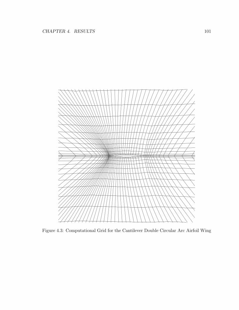
CHAPTER 4. RESULTS 101
Figure 4.3: Computational Grid for the Cantilever Double Circular Arc Airfoil Wing

CHAPTER 4. RESULTS 102
0 0.05 0.1 0.15 0.2 0.25 0.3
−1
−0.5
0
0.5
1
M = 0.795, q = 1.32 [psi]
Time [sec.]
Dis
plac
emet
[in.
]
0 0.05 0.1 0.15 0.2 0.25 0.3
−1
−0.5
0
0.5
1
M = 0.795, q = 1.34 [psi]
Time [sec.]
Dis
plac
emet
[in.
]
0 0.05 0.1 0.15 0.2 0.25 0.3
−1
−0.5
0
0.5
1
M = 0.795, q = 1.36 [psi]
Time [sec.]
Dis
plac
emet
[in.
]
Figure 4.4: Time History of the Displacements at the Mid-Chord of the Tip
CHAPTER 4. RESULTS 103
frequency of the vibration in the figure is faster than that of the first bending mode,
but it can be said that the vibration is dominated by the first bending mode and the
frequency change is a usual trend when a dynamic pressure approaches to the flutter
point. The second figure shows the structural response when the dynamic pressure
was changed from 1.32 psi to 1.34 psi. In this figure, the decay of the amplitude of the
tip deflection of the wing becomes quite a bit slower than the case of 1.32 psi and the
time history in the figure looks like an almost constant amplitude motion. This can be
recognized as the flutter point by the definition that flutter occurs when the damping
ratio of the response of the wing becomes less than zero. This time history can
be generated by an almost perfect balance between the unsteady aerodynamic loads
acting on the wing and the structural response of the wing in keeping a constant
amplitude of the vibration. The flutter frequency is higher than that of the first
bending mode, but the mode exhibiting the flutter is apparently the lowest frequency
mode, in this case the first bending mode, as is often the case. Finally, when the
dynamic pressure goes beyond the flutter point, the structural response consists of
a divergent vibration as seen in the case of 1.36 psi in Figure 4.4. Once flutter
occurs as seen in the figure, the structure would immediately fail due to the large
amplitude motion unless the flow condition around the wing changed significantly.
The experimental dynamic pressure measured at the flutter boundary for this Mach
number is 1.26 psi. In the same way, flutter boundaries for other Mach numbers are
detected by looking at time histories of the tip deflections of the wing.
Since the only parameter changed to detect the flutter boundaries is the dynamic
pressure, flutter boundaries can be shown on a figure where the corresponding dy-
namic pressures are plotted against Mach number. The results of the flutter bound-
aries determined by the computational responses are compared with the experiment
[94] in Figure 4.5. Each flutter point was determined as the dynamic pressure corre-
sponding to zero damping ratio based on a linear interpolation between one simulation
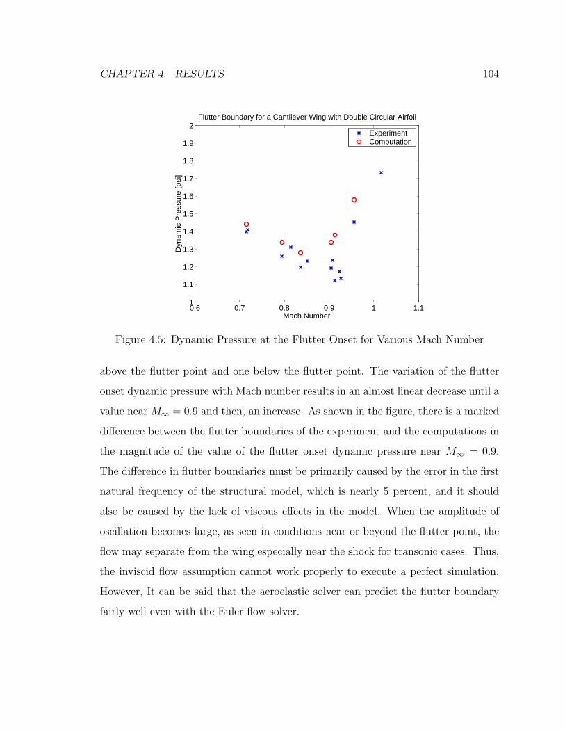
CHAPTER 4. RESULTS 104
0.6 0.7 0.8 0.9 1 1.11
1.1
1.2
1.3
1.4
1.5
1.6
1.7
1.8
1.9
2Flutter Boundary for a Cantilever Wing with Double Circular Airfoil
Mach Number
Dyn
amic
Pre
ssur
e [p
si]
ExperimentComputation
Figure 4.5: Dynamic Pressure at the Flutter Onset for Various Mach Number
above the flutter point and one below the flutter point. The variation of the flutter
onset dynamic pressure with Mach number results in an almost linear decrease until a
value near M∞ = 0.9 and then, an increase. As shown in the figure, there is a marked
difference between the flutter boundaries of the experiment and the computations in
the magnitude of the value of the flutter onset dynamic pressure near M∞ = 0.9.
The difference in flutter boundaries must be primarily caused by the error in the first
natural frequency of the structural model, which is nearly 5 percent, and it should
also be caused by the lack of viscous effects in the model. When the amplitude of
oscillation becomes large, as seen in conditions near or beyond the flutter point, the
flow may separate from the wing especially near the shock for transonic cases. Thus,
the inviscid flow assumption cannot work properly to execute a perfect simulation.
However, It can be said that the aeroelastic solver can predict the flutter boundary
fairly well even with the Euler flow solver.
CHAPTER 4. RESULTS 105
4.2 Flutter Analysis Demonstration - NASA Ro-
tor 67
4.2.1 NASA Rotor 67
The purpose of this study is to demonstrate the capability of the present analysis
program for predicting the flutter boundary of a realistic turbomachinery fan. As
pointed out in Chapter 1, supersonic flutter can occur even on the design speed line.
This type of flutter features strong shock oscillations and shock induced separations.
The potential interaction between these nonlinear flow features and the structural
response requires flutter explorations. Therefore, the goal of this study is to predict
the flutter boundaries in the compressor performance map, to examine the influence
of the inter-blade phase angle, and to observe how the flow field affects the instability
of the blade vibrations.
The selection of the configuration on which aeroelastic calculations are performed
is difficult due to the fact there is no turbomachinery rotor configuration whose geom-
etry, structural properties and experimental results for flutter boundaries are avail-
able in the open literature. Because of this the predictions presented here can not
demonstrate the accuracy of flutter boundary prediction. It is, however, hoped that
these calculations will be compared with other numerical predictions and become a
standard test case in this field.
NASA Rotor 67, the first stage rotor of the NASA Lewis (now NASA Glenn)
designed two-stage fan [96], has been recognized as a popular test case for three-
dimensional viscous flow prediction procedures because of the available detailed ex-
perimental data obtained using a laser anemometer [41]. In the early 1990’s, many re-
searchers reported steady flow predictions for this configuration [97, 98, 99, 100, 101].
Although the structural properties for this configuration are not available, the blade
is considered to be flexible enough for flutter to occur under some flow conditions.
CHAPTER 4. RESULTS 106
Rotor 67 has been used to validate aeroelastic applications by a few researchers.
Chuang and Verdon [102] applied their aeroelastic analysis code, called TURBO, to
this configuration. They examined the stability of the rotor blade in an inviscid flow
with the work per cycle responses to a prescribed blade vibration corresponding to a
reduced frequency of 0.54 based on the mid-span section. The reduced frequency, k,
is one of the most important parameters for flutter analysis defined by the following
expression.
k =cω
2Vref
. (4.1)
Here, ω is the frequency of the vibratory motion of the blade. For fans or compres-
sors, the relative inlet velocity at a certain blade section is chosen for Vref . The
variable c is the chord length of the corresponding blade section. Chuang and Verdon
showed the blade to be more stable when operating at the near stall point than at the
near peak efficiency point for a torsional mode. They also discussed the role of the
unsteady forces around the passage shock in determining the stability of the blade
motion. The location of the shock on the blade surface and the inter-blade phase
angle are especially thought to have a significant effect on whether the unsteady flow
extracts energy from the blade motion. L. He [40] has examined Rotor 67 vibrating
with a prescribed torsional mode with a Thin-layer Navier-Stokes aeroelastic solver.
The oscillation frequency had a reduced frequency of 1.5 based on the tip section.
He showed a significant effect of the viscous and tip clearance flow on the unsteady
torsional moments. As mentioned in Chapter 1, Vahdati, Imregun and their col-
leagues [52] performed a fluid/structure coupled aeroelastic computation for Rotor
67 with a Galerkin discretization of the fluid equations and ANSYS as the structural
solver. The reduced frequency of their calculations was 0.324 based on the tip section.
Their results show a rapid decay of the blade vibration at the near peak efficiency
operation point. Thus, Rotor 67 has been gaining in popularity as a test case among

CHAPTER 4. RESULTS 107
r = 9 cm
r = 26 cm
Tip Clearance = 0.1016 cm
Hub
Aero Station 1
x = −2.473 cm
x = 11.011 cm
x = 9.03 cm
Casing
Aero Station 2
x = 0
Figure 4.6: NASA Rotor 67
researchers interested in turbomachinery aeroelasticity in spite of the lack of available
data regarding its flutter characteristics. For these reasons, Rotor 67 was chosen for
the current investigation to demonstrate the capability of the previously described
nonlinear aeroelastic prediction procedure.
NASA Rotor 67 consists of 22 blades. The blade aspect ratio is 1.56. At the
design point, the rotational speed of the rotor is 16,043 RPM, with an inlet axial Mach
number of approximately 0.49, a tip inlet relative Mach number of 1.38, a tip speed
of 428.9 m/s, a total pressure ratio of 1.63 and a mass flow of 33.25 Kg/s. Figure
4.6 shows an overall view of Rotor 67 with a schematic detailing some important
dimensions. The rotor has a large amount of twist from hub to tip and the flow field
is extremely complex featuring a three-dimensional shock structure, shock-boundary
layer interaction, three-dimensional flow separation, and tip leakage flow.

CHAPTER 4. RESULTS 108
4.2.2 Computational Grid
Unsteady solutions are computed over single or multiple blade passages, depending on
the inter-blade phase angles. These computational domains are discretized to create
a multiblock structured computational grid. The grid used for the present study is
shown in Figure 4.7 with the meridional view and Figure 4.8 with the blade-to-blade
view. The grid for the single passage of Rotor 67 consists of 137 mesh points in the
stream-wise direction, 65 points in the blade-to-blade direction, and 81 points in the
span-wise direction. In the stream-wise direction, the grid extends one axial chord
upstream and downstream from the blade row at the hub, and has 33, 73 and 33
axial points along the upstream periodic boundary, in the blade passage and along
the downstream periodic boundary, respectively. A total of 17 points are used in the
span-wise direction to describe the tip-clearance between the rotor blades and the
casing.
The rotor has a 0.1016 cm tip clearance which makes the grid generation for a
structured multiblock code quite difficult. To take this into account, the grid in the
tip clearance region above the rotor tip is constructed by simply extending the blade
span to the casing, creating another block between the tip and the casing. The tip
clearance block is then discretized as shown in the Figure 4.9, making singular points
at the leading and trailing edges. The finite volume procedure can integrate the flux
going through the prismatic cells created at the leading and trailing edges simply
setting the projected face area at the singular points to zero. Boundary condition
treatment for these singular points is not required since the flux passing through these
points is zero.

CHAPTER 4. RESULTS 109
Figure 4.7: Meridional View of Computational Grid for NASA Rotor 67

CHAPTER 4. RESULTS 110
Figure 4.8: Blade-to-Blade View of Computational Grid for NASA Rotor 67
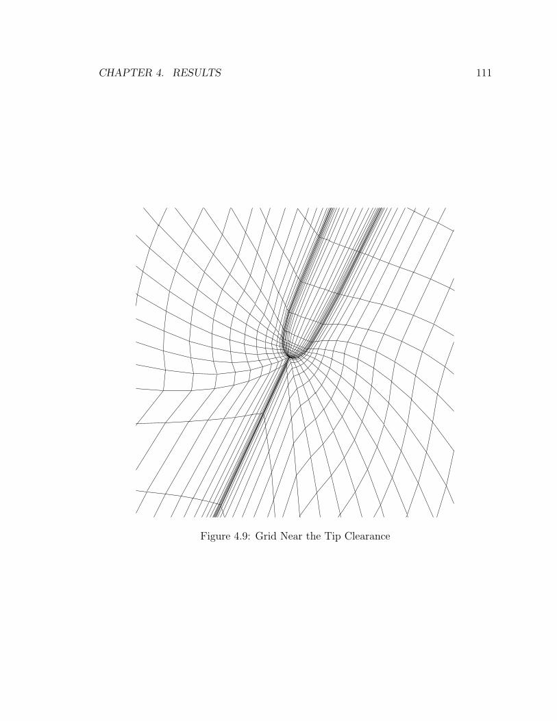
CHAPTER 4. RESULTS 111
Figure 4.9: Grid Near the Tip Clearance

CHAPTER 4. RESULTS 112
Figure 4.10: Finite Element Model of the NASA Rotor 67
4.2.3 Blade Structural Model
A NASTRAN finite element model was used to calculate direct transient structural
responses as well as to obtain the mode shapes and frequencies of the blade. The
model for the blade shown in Figure 4.10 consists of 11×11 nodes forming 200 trian-
gular plate elements with varying thickness. The thickness is distributed to match the
actual thickness of the blade. For structural boundary conditions, both translational
and rotational displacements are not allowed at the root of the blade.
Materials for blade construction are conventionally aluminum alloys, steel or stain-
less steel. However, in recent applications Titanium and later Beryllium have become
significant. In modeling NASA Rotor 67, an imaginary material is used, whose prop-
erties are shown in Table 4.1 with that of a titanium alloy. The Young’s modulus
and the density are chosen such that the first natural frequency becomes around 400
Hz. The reason why 400 Hz is chosen comes from the usual elastic design procedure
of rotor blades. The basic principle that needs to be satisfied in the design procedure

CHAPTER 4. RESULTS 113
Table 4.1: Material Properties
Young’s modules Poisson’s ratio Density
Titanium Alloy 1.172e+11 [Pa] 0.3 4539.5 [kg/m3]Current Material 1.422e+11 [Pa] 0.3 4539.5 [kg/m3]
is that resonant response between the blade mode and the rotation speed must be
avoided. The design rotation speed for Rotor 67 is 267.4 Hz and its double is 534.8
Hz. A typical first natural frequency of the blade is placed between these two numbers
to give adequate margin. However, as pointed out by Kielb [103], it is very difficult
to accomplish this for a solid titanium blade. In fact, if the blade of Rotor 67 was
modeled with a solid Titanium alloy with material properties described in the table,
the first frequency at the design speed would become 520 Hz which is very close to
the double of the rotation speed. Therefore, 400 Hz is picked as the first natural
frequency in order to keep a satisfactory margin with respect to the fundamental
frequency of revolution and its integer multiples.
The calculated mode shapes and modal frequencies for the Rotor 67 structural
model with the centrifugal stiffening included are shown in Figure 4.11 with their
frequencies. The blades are seen from the outer casing towards the axis of the rotor.
To obtain the mode shapes and frequencies, an eigenanalysis solution sequence 103 in
MSC/NASTRAN was used. In the figure, the blades drawn with thinner mesh lines
represent the original rigid shape of the blade, and the other solid pictures show the
corresponding mode shapes. The behavior of every mode is similar in terms of its
torsional motion near the root and bending motion near the tip. In addition, more
torsional components near the tip can be observed in the higher frequency modes
especially in the third and fourth mode.
For the design rotation speed of Rotor 67, the reduced frequency based on the

CHAPTER 4. RESULTS 114
(a) First Mode - 401.9 Hz (b) Second Mode - 1096.0 Hz
(c) Third Mode - 2093.7 Hz (d) Forth Mode - 2456.6 Hz
Figure 4.11: Mode Shape of the Rotor 67

CHAPTER 4. RESULTS 115
tip section becomes 0.27 according to the first mode frequency calculated with the
structural model by MSC/NASTRAN. Finally, for multi-passage simulations, the
cascade is assumed to be well tuned, which means that all the blades have identical
structural properties.
4.2.4 Steady Flow
Prior to performing the aeroelastic unsteady calculations, validation of the steady flow
solution needs to be performed such that the proper initial conditions for unsteady
calculations can be provided. In order to obtain an accurate representation of the
viscous flows around the rotor, the three-dimensional RANS equations are solved in
a relative non-Newtonian reference frame rotating with the blade. The k-ω model is
used to predict the turbulent eddy viscosity in the flow. Validation is conducted by
comparing the solutions with measurements taken with a laser anemometer [41] and
other RANS numerical simulations performed by numerous researchers. For example,
Chima [97] and Ha, et al. [98] gave detailed descriptions of the three-dimensional flow
structure around the blade. Jennions, et al. [99] and Adamczyk et al. [100] examined
the influence of the tip clearance by changing its size in the radial direction. Arnone
[101] described the complex nature of the transonic flow through Rotor 67 in detail.
Steady flow computations are performed with the measured total pressure, total
temperature and absolute flow angle profiles specified at the inlet and the measured
static pressure profile specified at the exit. Computations take approximately 2000
iterations with a CFL of 3 and three levels of a multigrid W-cycle to reach converged
solutions where the average density residual decreases by 3.5 orders of magnitude from
the initial conditions. The same CFL number is used for integrating the turbulence
model equations. The predicted solution at the near peak efficiency point is used
as initial conditions for all of the simulations which were run an additional 1000 to

CHAPTER 4. RESULTS 116
2000 iterations with different inlet and exit profiles depending on the operating point.
More iterations tend to be necessary for convergence for solutions closer to the stall
condition.
To show the ability of the flow solver to capture the correct performance, the
numerically calculated performance map of the rotor is shown in Figure 4.12 along
with the experimentally measured values. A total of 12 different operating conditions
were calculated to asses the overall accuracy in the numerical prediction of perfor-
mance. The adiabatic efficiency and total pressure ratio are calculated using the mass
averaged values of the total pressure and total temperature at the inlet and exit aero
survey stations shown in Figure 4.6. The adiabatic efficiency is defined as,
η =(Pt2/Pt1)
(γ−1)/γ − 1
(Tt2/Tt1)− 1, (4.2)
where Pt2 and Pt1 are the absolute total pressures at the inlet and exit respectively,
and Tt2 and Tt1 are the corresponding absolute total temperatures. The mass flow
in Figure 4.12 is nondimensionalized with respect to the choking mass flow. The
mass flow rate at the choke condition is found to be about 1.8 percent lower than
the experimentally observed value. An underprediction of the choked mass flow rate
is also reported in the other computational results [97, 99, 101]. As shown in Figure
4.12, the overall predicted performance of the compressor is in good agreement with
the experiment except for the following two areas. One area is that the computation
underpredicted the adiabatic efficiency for the peak efficiency point and also predicted
a lower mass flow rate. This trend was also predicted by Arnone [101]. The other area
is the obvious underpredicted absolute total pressure ratio. This underprediction is
likely due to an overprediction of shock and viscous flow losses and flow deviation.
However, the steady-state solution including the structural deformation mentioned
in the next section results in a higher mass flow and higher pressure ratio. Although
the structural model is not based on the real structure of Rotor 67, this suggests that

CHAPTER 4. RESULTS 117
0.92 0.94 0.96 0.98 10.82
0.84
0.86
0.88
0.9
0.92
0.94
Mass Flow Rate/Mass Flow Rate at Choke
Rot
or A
diab
atic
Effi
cien
cy
ExperimentComputation
0.92 0.94 0.96 0.98 11.3
1.4
1.5
1.6
1.7
1.8
Mass Flow Rate/Mass Flow Rate at Choke
Rot
or T
otal
Pre
ssur
e R
atio
ExperimentComputation
Figure 4.12: Comparison of Rotor Performance at Design Speed

CHAPTER 4. RESULTS 118
the underestimated pressure ratio and mass flow may be caused by the structural
deformation not included in the present calculations.
In particular, the experimental data reported in Strazisar’s document [41] con-
centrate on the near peak efficiency and near stall conditions. Detailed comparisons
between calculations and experiment are made at these two operating points. In Fig-
ure 4.13, the relative Mach number contours at three different span-wise locations,
i.e. 10, 30, and 70 percent span measured from the casing, are shown for the near
peak efficiency condition. Note that the contours are plotted on constant percent
radius surfaces, not on constant-radius surfaces. The relative Mach number at 10
percent of span is about 1.35. A bow shock at the leading edge and a normal in-
passage shock near the trailing edge on the suction surface can be observed. At 30
percent of the span, a lower Mach number, i.e., approximately 1.2, moves the in-
passage shock slightly forward but the shock structure is qualitatively similar. At 70
percent of the span, the inlet relative Mach number is subsonic, i.e., approximately
0.90, and a supersonic bubble appears near the leading edge on the suction surface.
The laser anemometer data is known to be uncertain in the center of the wake at
70 percent span, where computed data indicates a large region of separated flow. It
should be noted that the other computations also indicate flow separation on the
suction side near the hub. Figure 4.14 shows the radial survey of computed and mea-
sured mass-averaged thermodynamic parameter profiles downstream of the rotor for
peak efficiency operation. All the computed exit quantities agree very well with the
measurements.
Figures 4.15 and 4.16 show detailed results at an operating point near stall. Figure
4.15 shows a comparison of relative Mach number contours. The flow structure at the
near stall operating condition is similar to that for the near peak efficiency. While the
near peak condition generates two shocks, i.e. a bow shock at the leading edge and an
in-passage shock near the tip, a single detached bow shock is observed at the near stall

CHAPTER 4. RESULTS 119
0.9003
1.0804
0.76526
1.3593
1.40
31
1.00861.2062
1.3785
0.86159
From Casing10%Span
30% SpanFrom Casing
70%SpanFromCasing
Experiment Computation
Figure 4.13: Experimental and Numerical Relative Mach Number Contour for NearPeak Efficiency
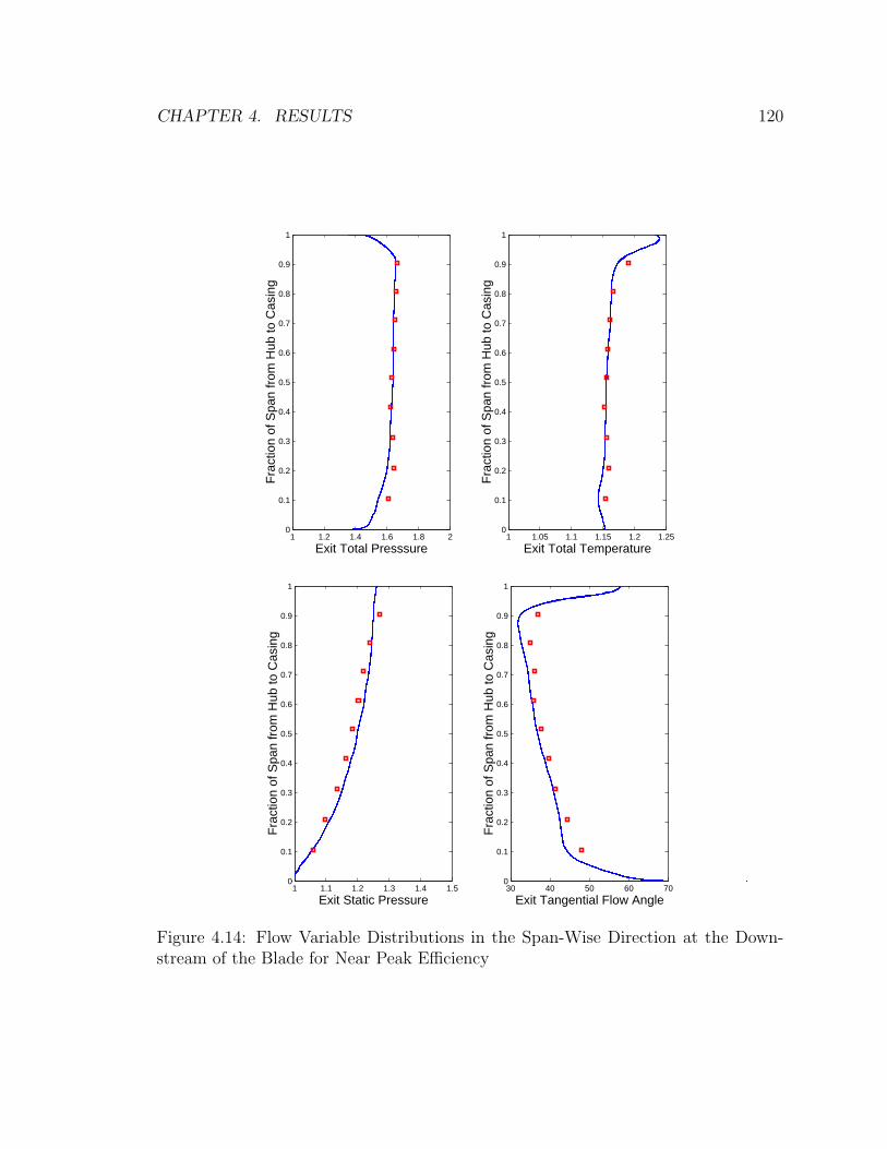
CHAPTER 4. RESULTS 120
1 1.2 1.4 1.6 1.8 20
0.1
0.2
0.3
0.4
0.5
0.6
0.7
0.8
0.9
1
Exit Total Presssure
Fra
ctio
n of
Spa
n fr
om H
ub to
Cas
ing
1 1.05 1.1 1.15 1.2 1.250
0.1
0.2
0.3
0.4
0.5
0.6
0.7
0.8
0.9
1
Exit Total Temperature
Fra
ctio
n of
Spa
n fr
om H
ub to
Cas
ing
1 1.1 1.2 1.3 1.4 1.50
0.1
0.2
0.3
0.4
0.5
0.6
0.7
0.8
0.9
1
Exit Static Pressure
Fra
ctio
n of
Spa
n fr
om H
ub to
Cas
ing
30 40 50 60 700
0.1
0.2
0.3
0.4
0.5
0.6
0.7
0.8
0.9
1
Exit Tangential Flow Angle
Fra
ctio
n of
Spa
n fr
om H
ub to
Cas
ing
Figure 4.14: Flow Variable Distributions in the Span-Wise Direction at the Down-stream of the Blade for Near Peak Efficiency
CHAPTER 4. RESULTS 121
condition. Thus, the pressure side is shock free. The computed shock is somewhat
more oblique than the measured shock especially at the 10 percent span location,
but the qualitative agreement is satisfactory. At 70 percent span, the supersonic
bubble is very similar, but again a large area of flow separation can be observed
in the computational results which does not appear in the experiment. Figure 4.16
compares radial surveys downstream of the rotor. All the computed parameters shown
in the figure agree well with the experimental results.
In general, the qualitative agreement between the experiments and computations
for both operating conditions is reasonably satisfactory, especially in the radial dis-
tribution of the thermodynamic quantities. As stated, the purpose of this study on
the steady-state solutions is to confirm the suitability of the flow solver and the com-
putational grid for an aeroelastic simulation. The results presented above indicate
that both are suitable for predicting the proper pressure loadings and shock positions.
Discrepancies between the computations and experiments are judged to be sufficiently
minor so as not to affect the conclusions obtained from the aeroelastic simulations
that follow.
4.2.5 Structure-Coupled Unsteady Flow
In this section, time dependent aeroelastic results are considered. The behavior of
the blade oscillation can be determined from forced response computations. In real-
ity, the blade-passing forced response is due to the excitation forces generated by the
rotation of the bladed system past a pressure field whose strength varies periodically
with the angular position of the rotor. Such flow variations are mainly caused by the
stator blades which act as upstream or downstream obstructions, and the fact that
the rotor blade experiences their wakes or potential field as time varying forces. In the
current computations, these periodic excitations can be simulated by impulsive initial

CHAPTER 4. RESULTS 122
1.4262
0.90337
1.1419
1.3175
0.79053
0.90194
0.6013
From Casing10%Span
30% SpanFrom Casing
70%SpanFromCasing
Experiment Computation
Figure 4.15: Experimental and Numerical Relative Mach Number Contour for NearStall

CHAPTER 4. RESULTS 123
1 1.2 1.4 1.6 1.8 20
0.1
0.2
0.3
0.4
0.5
0.6
0.7
0.8
0.9
1
Exit Total Presssure
Fra
ctio
n of
Spa
n fr
om H
ub to
Cas
ing
1.1 1.15 1.2 1.25 1.3 1.350
0.1
0.2
0.3
0.4
0.5
0.6
0.7
0.8
0.9
1
Exit Total Temperature
Fra
ctio
n of
Spa
n fr
om H
ub to
Cas
ing
1 1.1 1.2 1.3 1.4 1.50
0.1
0.2
0.3
0.4
0.5
0.6
0.7
0.8
0.9
1
Exit Static Pressure
Fra
ctio
n of
Spa
n fr
om H
ub to
Cas
ing
30 40 50 60 700
0.1
0.2
0.3
0.4
0.5
0.6
0.7
0.8
0.9
1
Exit Tangential Flow Angle
Fra
ctio
n of
Spa
n fr
om H
ub to
Cas
ing
Figure 4.16: Flow Variable Distributions in the Span-Wise Direction at the Down-stream of the Blade for Near Stall
CHAPTER 4. RESULTS 124
displacements given to the blade. As previously shown, the steady-state solutions can
be obtained for the rigid unloaded blade geometry. Prior to the aeroelastic response
calculations, the blade is allowed to move and dynamically relax to a steady-state
loaded condition. The influence of centrifugal forces and fluid pressure causes the
blade’s steady-state loaded geometry to be different from its original unloaded geom-
etry. Then, the blade is deformed an additional amount predominantly corresponding
to the first mode. The amplitude of the blade initial deflection is about 30 percent of
the deflection under steady load. Once the new steady solution for the blade with the
initial deformations obtained, the blade is released and allowed to move according to
the aeroelastic interaction.
The periodicity of the exciting forces is primarily determined by the ratio between
the number of upstream or downstream stator blades and that of rotor blades. This
periodicity results in blade vibrations propagating in the direction of rotation with a
constant inter-blade phase angle σ between adjacent blades. In the solution procedure,
a constant inter-blade phase angle is determined by the initial displacements and
velocities for multi-passage computations. In addition, the inter-blade phase angle
is forced by the periodicity boundary condition. For example, consider the case of
σ=180 degrees. The computation needs to be performed with two passages where
one blade is given an initial displacement and zero initial velocity and the other is
given the initial displacement in the opposite direction with the same amplitude and
zero initial velocity as well. The aerodynamic force arising from the blade vibration
introduces an aerodynamic damping that can be either positive or negative, depending
on the operating points and the phase angle of vibration. To investigate the effect of
inter-blade phase angle, calculations for four different inter-blade phase angles shown
in Table 4.2 were performed at the near peak efficiency point. In addition, two inter-
blade phase angles at a near stall operation point corresponding to the pressure ratio
of 1.69 and at a near choke point with a pressure ratio of 1.5 were selected to examine

CHAPTER 4. RESULTS 125
Table 4.2: Case Matrix for Rotor 67 Aeroelastic Calculations
Operating Point Pressure Ratio Inter-Blade Phase Angle σ
Near Peak Efficiency 1.63 0 deg90 deg180 deg270 deg
Near Stall 1.69 0 deg180 deg
Near Choke 1.50 0 deg180 deg
the effect on the flow field structure, especially the shock strength and its location.
Five cycles of oscillation, which result in about 0.02 seconds of real time, were
found to be sufficient to distinguish whether the oscillation decays or grows. A total
of 36 time steps per vibration period of the first oscillation mode was chosen in order
to ensure the accuracy of the coupled system with the dual time stepping scheme
and the Newmark scheme. Between 40 to 60 W-cycle multigrid cycles per physical
time step were necessary to provide a reasonable time-accurate pressure distribution
to the structural model. These numbers were carefully determined from numerical
experiments to avoid large deviations in the structural response due to the pressure
fields being still in transition [95].
Flutter stability is assessed from the time history of the displacements. Figure 4.17
shows the variation of the circumferential direction displacements of the blade with
time for σ = 0 and 180 degrees at the near peak efficiency point. The displacements
are defined as the deflections from the original rigid shape of the structure. The
displacements shown in the figure are measured at the mid-chord of the tip section.
Since there is no chance that a node of one of the dominant modes shown in Figure 4.11
lies at the mid-chord of the tip section, . These displacement measurements would
never miss the displacements due to the dominant modes. For σ = 180 degrees, only

CHAPTER 4. RESULTS 126
0 0.005 0.01 0.0150.11
0.12
0.13
0.14
0.15
0.16
0.17
0.18Blade1, ω = 16043[rpm], P2/P1 = 1.63
Time [sec.]
Dis
plac
emet
[in.
]
(a) σ = 0 deg.
0 0.005 0.01 0.0150.11
0.12
0.13
0.14
0.15
0.16
0.17
0.18Blade1, ω = 16043[rpm], P2/P1 = 1.63
Time [sec.]
Dis
plac
emet
[in.
](b) σ = 180 deg.
Figure 4.17: Deflection at the Mid-Chord of the Tip Section for Near Peak Efficiency,σ = 0, 180 deg
the motion of one blade is shown. The motion of the other blade is similar except
that the displacements are in the opposite direction. The response for σ = 0 degrees
shows almost a typical forced response with constant amplitude of oscillation. On the
other hand, the response for σ = 180 degree shows decreasing amplitude with each
oscillation cycle, indicating a decay in the oscillation and a flutter free condition.
Thus the aerodynamic damping for σ = 180 degree is much greater than that for σ
= 0 degree.
To investigate the stability for other inter-blade phase angles, calculations were
started from the initial displacements and velocities corresponding to σ = 90 and 270
using four passages. Figure 4.18 illustrates the responses for these inter-blade phase
angles. When the inter-blade phase angle is positive, the wave of blade vibrations of
a fan rotor travels in the direction of rotation as shown in Figure 1.2. In practice, a
greater than 180 degree inter-blade angle produces a wave traveling in the opposite
direction. All the results shown in the figure indicate decaying curves of the aeroelastic

CHAPTER 4. RESULTS 127
0 0.002 0.004 0.006 0.008 0.01 0.0120.11
0.12
0.13
0.14
0.15
0.16
0.17
0.18Blade1, ω = 16043[rpm], P2/P1 = 1.63
Time [sec.]
Dis
plac
emet
[in.
]
(a) σ = 90 deg.
0 0.002 0.004 0.006 0.008 0.01 0.0120.11
0.12
0.13
0.14
0.15
0.16
0.17
0.18Blade1, ω = 16043[rpm], P2/P1 = 1.63
Time [sec.]
Dis
plac
emet
[in.
](b) σ = 270 deg.
Figure 4.18: Deflection at the Mid-Chord of the Tip Section for Near Peak Efficiency,σ = 90, 270 deg
response. These results implies that the inter-blade phase angle which produces the
least stable response may exist near σ = 0 degrees.
To examine how the unsteady pressure influences the stability of the blade motion,
the unsteady pressure may be decomposed by a Fourier analysis into the components
contributing and not contributing to the damping. Figure 4.19 shows the calculated
distribution of the first harmonic imaginary unsteady pressure along with the distri-
bution of the mean value of the unsteady pressure on the suction and pressure sides,
respectively. The results are presented for σ = 0 degrees. The mean surface pressures
in Figure 4.19 are obtained by averaging the unsteady pressures over the last oscil-
lation cycle. The first harmonic imaginary components of the pressure perturbations
are supposed to act in accordance with damping terms.
As shown, significant unsteady pressure amplitudes exist in the region where the
shocks sit on the blade. On the suction side, the shock appears along the entire span as
a continuous line. However, the imaginary pressure distribution shows the peak along

CHAPTER 4. RESULTS 128
(b) 1st Harmonic Imaginary Value
(d) 1st Harmonic Imaginary Value
(a) Mean Value − Suction Side
(c) Mean Value − Pressure Side
supersonic bubbleShock in
−Sucsion Side
−Pressure Side
In−passage shockpropagates fromthe suction side
In−passage shock
In−passage shock
Figure 4.19: Unsteady Pressure Distribution on the Blade Surfaces for Near PeakEfficiency, σ = 0 deg

CHAPTER 4. RESULTS 129
the shock is split into two parts. Between the casing and 40 percent of the span, the
passage shock is very strong and indicates that an adverse pressure gradient follows
that may cause shock induced separation. On the other hand, below 40 percent of
span, the shock is formed inside the supersonic bubble and does not reach the pressure
side of the adjacent blade as seen in the Mach contour at the 70 percent span location
in Figure 4.13. These two kinds of shocks behave differently as damping forces. While
the in-passage shock generates a negative peak in the imaginary pressure distribution,
the shock in the supersonic bubble generates a positive peak. On the pressure side,
the imaginary pressure distribution also indicates peaks along the in-passage shock
near the leading edge. In addition, it is shown that the in-passage shock on the suction
side propagates over the tip clearance to the pressure side of the blade around the
middle chord near the tip. This small shock generates another peak in the unsteady
pressure as well.
Figure 4.20 shows the mean and first harmonic imaginary pressure distributions
for σ = 180 degrees. The results show that considerably larger unsteady forces arise
when the motion of adjacent blades is out of phase. For this case, the two kinds of
shocks on the suction side mentioned above do not form a continuous line, and the
oblique shock from the leading edge of the adjacent blade strikes more prominently
near the tip on the suction side. In particular, the in-passage shock on the suction
side shows a totally different peak of the unsteady pressure, although the other shocks
on the suction side do not generate peaks.
Now that it has been shown that the shock oscillations generate large pressure
fluctuations, the next question will be whether these fluctuations damp or excite the
blade motion. To examine this, the work per cycle is a parameter often used to
represent the contributions of unsteady pressure fields to the stability of the blade
motion. The work per cycle, WC , is the work done by the fluid on a given blade over
one cycle of its motion. It is obtained by computing the product of the pressure force

CHAPTER 4. RESULTS 130
(b) 1st Harmonic Imaginary Value
(d) 1st Harmonic Imaginary Value
(a) Mean Value − Suction Side
(c) Mean Value − Pressure Side
−Sucsion Side
−Pressure Side
supersonic bubbleShock in
In−passage shock
Oblique shock
Figure 4.20: Unsteady Pressure Distribution on the Pressure Side for Near PeakEfficiency, σ = 180 deg

CHAPTER 4. RESULTS 131
and the associated differential displacement.
WC =
∫ t+T
t
∫
∂Ω
p(x, y, z, t)q(x, y, z, t) · dSdt. (4.3)
In this equation, negative work implies positive damping in which aerodynamic forces
act in the opposite direction of the velocity of the displacements. Therefore, a blade
motion is stable, neutrally stable, or unstable according to whether the work per
cycle is less than, equal to, or greater than zero, respectively. Figures 4.21 and 4.22
show the aerodynamic work per cycle of the last period for σ = 0 and 180 degrees,
respectively. For σ = 0 degrees, a negative peaks appear at the locations where the
oblique shock and the lower part of the shock sit on the suction side. Therefore, the
oblique shock and the lower shock oscillations work to dampen the blade motion. On
the pressure side, there is a positive peak near the location of the in-passage shock.
Notice that the regions of exciting and damping forces on both sides are quite close.
That means that the exciting and damping forces generated by the shock oscillations
cancel each other resulting in an almost constant amplitude motion. On the other
hand, the distributions for σ = 180 degrees show that the forces generated by the
in-passage shock on the suction side works to dampen the oscillation, while the peaks
along the oblique shock and the lower part of the shock disappear. For this case
almost the entire suction side is associated with damping forces. Is is also obvious
that the in-passage shock on the pressure side produces a large damping force toward
the leading edge. Thus the physical mechanism for the decaying response of the σ
= 180 case is clearly explained. It is also implied in this discussion that the phase
change of the imaginary part of the unsteady pressure is associated with stabilization
or destabilization of the oscillation.
In order to validate the arguments developed so far, two other operation points
were chosen to examine the effect of a different kind of shock structure. One is a near

CHAPTER 4. RESULTS 132
(a) Suction Side (b) Pressure Side
Figure 4.21: Work per Cycle Distribution on the Blade Surface for Near Peak Effi-ciency, σ = 0 deg

CHAPTER 4. RESULTS 133
(a) Suction Side (b) Pressure Side
Figure 4.22: Work per Cycle Distribution on the Blade Surface for Near Peak Effi-ciency, σ = 180 deg

CHAPTER 4. RESULTS 134
0 0.005 0.010.11
0.12
0.13
0.14
0.15
0.16
0.17
0.18Blade1, ω = 16043[rpm], P2/P1 = 1.69
Time [sec.]
Dis
plac
emet
[in.
]
(a) σ = 0 deg.
0 0.005 0.010.11
0.12
0.13
0.14
0.15
0.16
0.17
0.18Blade1, ω = 16043[rpm], P2/P1 = 1.69
Time [sec.]
Dis
plac
emet
[in.
](b) σ = 180 deg.
Figure 4.23: Deflection at the Mid-Chord of the Tip Section for Near Stall, σ =0, 180 deg
stall operating point corresponding to a total pressure ratio of 1.69, and the other is
a near choke operating point corresponding to a total pressure ratio of 1.5.
As shown in Section 4.2.4, a detached bow shock is formed near the tip and the
pressure side is shock-free at the near stall operating point. Figure 4.23 shows the
aeroelastic responses for σ = 0 and 180 degrees at the near stall point. Similarly to the
near peak efficiency point, while the response for σ = 0 degrees shows an oscillation
with an almost constant amplitude, the response for σ = 180 degree shows a decaying
oscillation. Again, the aerodynamic damping for σ = 180 degrees is greater than that
for σ = 0 degrees.
In order to investigate the locations of strong damping effects, the work per cycle
was calculated for these cases too. Figure 4.24 shows the work per cycle distributions
for the near stall operating condition cases. A similar trend to the near peak efficiency
case can be seen on the suction surface. While the lower shock stabilizes the motion,
the bow shock sitting near the tip region excites the blade motion. Since the shock
CHAPTER 4. RESULTS 135
wave near the tip region doesn’t sit on the pressure side for the near stall case, no
major peak in the work per cycle can be seen on the pressure surface.
Figure 4.25 shows the Mach contours for the near choke case. The in-passage shock
is much stronger and extends from the middle of the pressure side to the trailing edge
on the suction side. The oblique shock generated at the leading edge near the tip
region reaches the suction side of the adjacent blade. Even at the 70 percent span
station, not only the supersonic bubble, but also the shock near the middle of the
chord can be observed.
Figure 4.27 shows the work per cycle distributions for the near choke case. From
the picture of the suction side for σ = 0 degrees, it is implied that the shock inside
the supersonic bubble near the hub has developed to form the oblique shock toward
the tip region. The oblique shock also reaches the pressure side of the adjacent
blade. Similarly to the near peak efficiency cases, the in-passage shock produces
an excitation force on the upper part of the suction surface for σ = 0 degree case.
On the other hand, the pressure surface experiences damping forces from the in-
passage shock which cancel the exciting force on the suction side. When the cascade
has an inter-blade phase angle of 180 degrees, the peak on the suction side due to
the in-passage shock disappears. Although exciting forces appear on the pressure
side instead, the damping forces due to the in-passage shock and the oblique shock
dominate the stability.
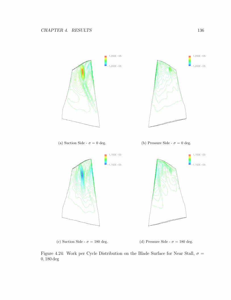
CHAPTER 4. RESULTS 136
(a) Suction Side - σ = 0 deg. (b) Pressure Side - σ = 0 deg.
(c) Suction Side - σ = 180 deg. (d) Pressure Side - σ = 180 deg.
Figure 4.24: Work per Cycle Distribution on the Blade Surface for Near Stall, σ =0, 180 deg
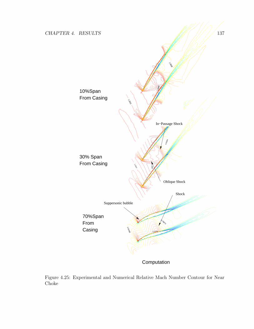
CHAPTER 4. RESULTS 137
0.92485 1.1771
0.79873
1.2247
1.3997
0.91
854
1.3501
1.49
48
1.0608
Suppersonic bubble
Oblique Shock
In−Passage Shock
Shock
From Casing10%Span
30% SpanFrom Casing
70%SpanFromCasing
Computation
Figure 4.25: Experimental and Numerical Relative Mach Number Contour for NearChoke

CHAPTER 4. RESULTS 138
0 0.005 0.01 0.0150.1
0.11
0.12
0.13
0.14
0.15
0.16Blade1, ω = 16043[rpm], P2/P1 = 1.5
Time [sec.]
Dis
plac
emet
[in.
]
(a) σ = 0 deg.
0 0.005 0.01 0.0150.1
0.11
0.12
0.13
0.14
0.15
0.16Blade1, ω = 16043[rpm], P2/P1 = 1.5
Time [sec.]
Dis
plac
emet
[in.
]
(b) σ = 180 deg.
Figure 4.26: Deflection at the Mid-chord of the Tip Section for Near Choke, σ =0, 180 deg

CHAPTER 4. RESULTS 139
(b) Pressure Side − 0 deg.
(d) Pressure Side − 180 deg.
(a) Suction Side − 0 deg.
(c) Suction Side − 180 deg.
Peak alongthe in−passage shock
Peak alongthe oblique shock
Peak alongthe in−passage shock
In−passage shock
Figure 4.27: Work per Cycle Distribution on the Blade Surface for Near Choke,σ = 0, 180 deg
Chapter 5
Conclusions and Future Work
A fluid/structure coupled aeroelastic solver for turbomachinery based on a three-
dimensional unsteady RANS solver, TFLO, and the finite element structural analysis
package, MSC/NASTRAN, was developed for use in turbomachinery flutter simula-
tions. The capabilities of the solver are demonstrated by applying it to investigate the
forced response characteristics of a transonic fan rotor, NASA Rotor 67. The aeroe-
lasitic solver successfully produces decaying or growing responses of the structural
motion for turbomacninery depending on the flow conditions, i.e. operating points
and inter-blade phase angles. Calculations were also carried out for an isolated wing
in transonic flow.
Results presented for Rotor 67 revealed that the main contribution to the stability
of a transonic fan is in the unsteady forces generated by the shock motions. In
determining these shock motions, inter-blade phase angles play the most important
role. The phase angle between the blade motion and the shock motion determines
whether the unsteady forces behave to damp or excite the oscillations. For detecting
the source of the exciting forces, work per cycle distributions on the blade surfaces
are very useful. One of the greatest benefits of a fluid/structure coupling solution
procedure is found to be the ability to visualize the phenomena, including the blade
140

CHAPTER 5. CONCLUSIONS AND FUTURE WORK 141
motion, which can aid in developing a methodology to avoid the instabilities by
modifying the blade shape or its structure.
It should be noted that difficulties in obtaining an unsteady aeroelastic response
are often associated with the calculation of the steady-state flow. The lessons learned
here are that if difficulties in convergence are encountered in the unsteady calcula-
tions, the initial steady-state solution would be suspicious. It might be a solution in
the middle of a steady-state calculation which would eventually diverge. A proper
level of convergence for the initial steady-state solution is one of the most important
factors for a successful unsteady computation in which a large amount of iterations
follow the computation for obtaining the initial condition. In order to obtain a con-
verged initial solution, a proper choice of turbulence model and an accurate treatment
of the geometry of the tip clearance region are important in turbomachinery compu-
tations. In the tip clearance region, the mixture of extremely nonlinear transonic flow
and heavy shear flow characteristics causes rapid variations in solutions which would
require the proper modelings of the tip clearance for stable computations. Further-
more, these modelings would affect the stability in unsteady computations because
the mesh in this region is the most sensitive in keeping its original quality during
mesh perturbations as mentioned in Section 3.1.8.
One of the biggest concerns for these fluid/structure computations is that the cou-
pled procedure is still computationally expensive. The prediction of flutter boundaries
with approaches such as time-linearized methods may be useful for single blade rows.
Advanced engines, however, will likely require aeroelastic analysis for multiple blade
rows, or a whole wheel system to admit all possible frequencies and inter-blade phase
angles. Fluid/structure couplings such as the one presented here would contribute to
these kinds of numerical predictions for aeroelastically severe conditions. In addition,
numerical analysis of aeroelastically related phenomena in turbomachinery such as
flutter, rotating stall, inlet distortion, mistunings, etc. will be less expensive than the

CHAPTER 5. CONCLUSIONS AND FUTURE WORK 142
experimental validations. Furthermore, one of the biggest benefits of the numerical
analysis is its richness in data that the experiment has been lacking due the difficulties
in installing the measurement instruments.
Whole system analyses will be required for making reliable blade and aeroelastic
response predictions. As far as the structural modeling is concerned, such analyses
must include multi-component coupling, such as blade-disk and disk-rotor interac-
tions and support system flexibilities. Mechanical damping in turbomachines occurs
during rubbing at mating interfaces: shroud, root, blade-to-blade or blade-to-disk
dampers. More accurate modeling of mechanical damping will be needed for making
better aeroelastic predictions. In addition, the modeling of gyroscopic terms will be
a problem that should be solved.

Bibliography
[1] E. H. Dowell, H. C. Curtiss, R. H. Scanlan, and F. Sisto. A Modern Course in
Aeroelasticity, chapter 8, pages 411–442. Kluwer Academic Publishers, 1989.
[2] F. Sisto. A Survey of Current Problems in Turbomachine Aeroelasticity. In
Recent Trends in Aeroelasticity, Structures, and Structural Dynamics, pages
48–62. University Press of Florida, 1986.
[3] E. Szechenyi. Understanding Fan Blade Flutter Through Linear Cascade.
In AGARD Manual on Aeroelasticity in Axial-Flow Turbomachines, number
AGARDograph No. 298, chapter 1-10. 1987.
[4] D. G. Halliwell. Effect of Intake Conditions on Supersonic Unstalled Flutter in
Turbofan Engines. Journal of Aircraft, 17(5):300–304, May 1980.
[5] O. O. Bendiksen. Role of Shocks in Transonic/Supersonic Compressor Rotor
Flutter. AIAA Journal, 24(7):1179–1186, July 1986.
[6] H. Stargardter. Fan Flutter Test. In AGARD Manual on Aeroelasticity in Axial-
Flow Turbomachines, number AGARDograph No. 298, chapter 2-10. 1987.
[7] D. S. Whitehead. Classical Two-Dimensional Methods. In AGARD Manual on
Aeroelasticity in Axial-Flow Turbomachines, number AGARDograph No. 298,
chapter 1-3. AGARD, 1987.
[8] O. O. Bendiksen. Aeroelastic Problems in Turbomachines. In Flight-Vehicle
Materials, Structures, and Dynamics, volume 5 of 2, chapter 5, pages 241–297.
ASME, 1993.
143

BIBLIOGRAPHY 144
[9] J. M. Verdon. Review of Unsteady Aerodynamic Method for Turbomachin-
ery Aeroelastic and Aeroacoustic Applications. AIAA Journal, 31(2):235–250,
February 1993.
[10] F. O. Carta. Coupled Blade-Disk-Shroud Flutter Instabilities in Turbojet En-
gine Rotors. Journal of Engineering for Power, 89(3):419–426, July 1967.
[11] D. S. Whitehead. Force and Moment Coefficients for Vibrating Aerofoils in Cas-
cade. Technical Report Reports and Memoranda 3254, Aeronautical Research
Council, February 1960.
[12] D. S. Whitehead. Bending Flutter of Unstalled Cascade Blades at Finite Deflec-
tion. Technical Report Reports and Memoranda 3386, Aeronautical Research
Council, October 1962.
[13] H. Atassi and T. J. Akai. Aerodynamic and Aeroelastic Characteristics of Os-
cillating Loaded Cascades at Low Mach Number Part 1: Pressure Distribution,
Forces, and Moments. Journal of Engineering for Power, 102(2):344–351, April
1980.
[14] T. J. Akai and H. Atassi. Aerodynamic and Aeroelastic Characteristics of
Oscillating Loaded Cascades at Low Mach Number Part 2: Stability and Flutter
Boundary. Journal of Engineering for Power, 102(2):352–356, April 1980.
[15] F. Lane and M. Friedman. Theoretical Investigation of Subsonic Oscillatory
Blade-Row Aerodynamics. Technical Report NACA-TN-4136, February 1958.
[16] S. N. Smith. Discrete Frequency Sound Generation in Axial Flow Turboma-
chines. Technical Report Reports and Memoranda 3709, Aeronautical Research
Council, March 1972.
[17] M. Namba. Subsonic Cascade Flutter with Finite Mean Lift. AIAA Journal,
13(5):586–593, May 1975.
[18] J. M. Verdon and J. E. McCune. Unsteady Supersonic Cascade in Subsonic
Axial Flow. AIAA Journal, 13(2):193–201, February 1975.

BIBLIOGRAPHY 145
[19] T. Nagashima and D. S. Whitehead. Linearized Supersonic Unsteady Flow
in Cascades. Technical Report Reports and Memoranda 3811, Aeronautical
Research Council, February 1977.
[20] M. E. Goldstein, W. Braun, and J. J. Adamczyk. Unsteady Flow in a Supersonic
Cascade with Strong In-Passage Shocks. Journal of Fluid Mechanics, 83(3):569–
604, December 1977.
[21] M. Namba and A. Ishikawa. Three-Dimensional Aerodynamic Characteristic of
Oscillating Supersonic and Transonic Annular Cascades. Journal of Engineering
for Power, 105(2):138–146, January 1983.
[22] J. M. Verdon and J. R. Casper. A Linearized Unsteady Aerodynamic Analysis
for Transonic Cascades. Journal of Fluid Mechanics, 149:403–429, 1984.
[23] D. S. Whitehead. A Finite Element Solution of Unsteady Two-Dimensional
Flow in Cascades. International Journal for Numerical Methods in Fluids,
10:13–34, 1990.
[24] K. C. Hall and E. F. Crawley. Calculation of Unsteady Flows in Turbomachinery
Using Linearized Euler Equations. AIAA Journal, 27(6):777–787, June 1989.
[25] K. C. Hall and C. B. Lorence. Calculation of Three-Dimensional Unsteady Flows
in Turbomachinery Using the Linearized Harmonic Euler Equations. Journal
of Turbomachinery, 115(4):800–809, October 1993. ASME-92-GT-136.
[26] W. Ning and L. He. Computation of Unsteady Flows Around Oscillating Blades
Using Linear and Nonlinear Harmonic Euler Methods. Journal of Turbomachin-
ery, 120(3):508–514, July 1998. ASME-97-GT-229.
[27] R. H. Ni and F. Sisto. Numerical Computation of Nonstationary Aerodynamics
of Flat Plate Cascades in Compressible Flow. Journal of Engineering for Power,
98(2):165–170, April 1976.
BIBLIOGRAPHY 146
[28] T. H. Fransson and M. Pandolfi. Numerical Investigation of Unsteady Subsonic
Compressible Flows through an Oscillating Cascade. In ASME 31st Interna-
tional Gas Turbine Conference and Exhibit, June 1986.
[29] G. A. Gerolymos. Numerical Integration of the Blade-to-Blade Surface Euler
Equations in Vibrating Cascades. AIAA Journal, 26(12):1483–1492, December
1988.
[30] L. He. An Euler Solution for Unsteady Flows Around Oscillating Blades. Jour-
nal of Turbomachinery, 115(4):714–722, October 1990. ASME-89-GT-279.
[31] J. I. Erdos, E. Alzer, and W. McNally. Numerical Solution of Periodic Transonic
Flow through a Fan Stage. AIAA Journal, 15(11):1559–1568, November 1975.
[32] G. A. Gerolymos. Advances in the Numerical Integration of the Three-
Dimensional Euler Equations in Vibrating Cascades. Journal of Turbomachin-
ery, 115(4):781–790, October 1993. ASME-92-GT-170.
[33] D. Peitsch, H. E. Gallus, and S. Weber. Computation of Unsteady Transonic 3D-
Flow in Turbomachine Bladings. In Unsteady Aerodynamics and Aeroelasticity
of Turbomachines, pages 161–176. Elsevier, 1995.
[34] R. W. MacCormack. Numerical computation of compressible viscous flow.
Course Reader of AA214 Stanford University, 1995.
[35] D. L. Huff. Numerical Simulations of Unsteady, Viscous, Transonic Flow Over
Isolated and Cascaded Airfoils Using a Deforming Grid. In AIAA 19th Fluid
Dynamics, Plasma Dynamics and Lasers Conference, number AIAA-87-1316,
June 1987.
[36] L. D. G. Siden. Numerical simulation of unsteady viscous compressible flows
applied to blade flutter analysis. In ASME 36th International Gas Turbine and
Aeroengine Congress and Exposition, number ASME-91-GT-203, June 1991.

BIBLIOGRAPHY 147
[37] L. He and J. D. Denton. Inviscid-Viscous Coupled Solution for Unsteady Flows
Through Vibrating Blades: Part 1 - Description of the Method. Journal of
Turbomachinery, 115(1):94–100, January 1993. ASME-91-GT-125.
[38] L. He and J. D. Denton. Inviscid-Viscous Coupled Solution for Unsteady Flows
Through Vibrating Blades: Part 2 - Computational Results. Journal of Turbo-
machinery, 115(1):101–109, January 1993. ASME-91-GT-126.
[39] S. Ji and F. Liu. Flutter Computation of Turbomachinery Cascades Using a
Parallel Unsteady Navier-Stokes Code. AIAA Journal, 37(3):320–327, March
1999.
[40] L. He and J. D. Denton. Three-Dimensional Time-Marching Inviscid and Vis-
cous Solutions for Unsteady Flows Around Vibrating Blades. Journal of Tur-
bomachinery, 116(3):469–476, July 1994. ASME-93-GT-92.
[41] A. J. Strazisar, J. R. Wood, M. D. Hathaway, and K. L. Suder. Laser Anemome-
ter Measurements in a Transonic Axial-Flow Fan Rotor. Technical Report
NACA-TP-2879, 1989.
[42] M. A. Bakhle, R. Srivastava, Jr. T. G. Keith, and G. L. Stefko. A 3D
Euler/Navier-Stokes Aeroelastic Code for Propulsion Applications. In AIAA
33rd AIAA/ASME/SAE/ASEE Joint Propulsion Conference and Exhibit, num-
ber AIAA-97-2749, July 1997.
[43] B. S. Baldwin and H. Lomax. Thin Layer Approximation and Algebraic Model
for Separated Turbulent Flows. In AIAA 16th Aerospace Sciences Meeting,
number AIAA-78-257, January 1978.
[44] P. A. Storey. Holographic Vibration Measurement of a Rotating Fluttering
Fan. In Proceedings of AIAA/SAE/ASME 18th Joint Propulsion Conference,
number AIAA-82-1271, June 1982.
[45] D. S. Whitehead. Torsional Flutter of Unstalled Cascade Blades at Zero Deflec-
tion. Technical Report Reports and Memoranda 3429, Aeronautical Research
Council, March 1964.
BIBLIOGRAPHY 148
[46] O. O. Bendiksen and P. Friedmann. Coupled Bending Torsion Flutter in Cas-
cades. AIAA Journal, 18(2):194–201, February 1980.
[47] R. L. Bispringhoff, H. Ashley, and R. L. Halfman. Aeroelasticity. Addison-
Wesley, 1955.
[48] K. Rao, V. Kaza, and R. E. Kielb. Flutter of Turbofan Rotor with Mistuned
Blades. AIAA Journal, 22(11):1618–1625, November 1984.
[49] G. A. Gerolymos. Coupled Three-Dimensional Aeroelastic Stability Analysis
of Bladed Disks. Journal of Turbomachinery, 115(4):791–799, October 1993.
ASME-92-GT-171.
[50] T. S. R. Reddy, M. A. Bakhle, D. L. Huff, and T. W. Swafford. Analysis of
Cascades Using a Two-Dimensional Euler Aeroelastic Solver. In Proceedings
of AIAA/ASME/ASCE/AHS/ASC 33rd Structures, Structural Dynamics and
Material Conference, number AIAA-92-2370, April 1992.
[51] L. He. Rotating-Stall/Stall-Flutter prediction Using A Fluid/Structure Coupled
Method. In Unsteady Aerodynamics and Aeroelasticity of Turbomachines, pages
597–607. Elsevier, 1995.
[52] M. Vahdati and M. Imregun. Nonlinear Aeroelasticity Analysis Using Unstruc-
tured Dynamics Meshes. In Unsteady Aerodynamics and Aeroelasticity of Tur-
bomachines, pages 177–196. Elsevier, 1995.
[53] J. W. Chew, J. G. Marshall, M. Vahdati, and M. Imregun. Part-Speed Flutter
Analysis of a Wide-Chord Fan Blade. In Unsteady Aerodynamics and Aeroelas-
ticity of Turbomachines, pages 707–724. Kluwer Academic Publisher, 1998.
[54] D. A. Gottfried and S. Fleeter. Aerodynamic Damping Predictions for Tur-
bomachine Blade Rows Using a Three-Dimensional Time Marching Simulation.
In AIAA/ASME/SAE/ASEE Joint Propulsion Conference and Exhibit, number
AIAA-99-2810, June 1999.
BIBLIOGRAPHY 149
[55] H. Doi and J. J. Alonso. Fluid/Structure Coupled Aeroelastic Computations
for Transonic Flows in Turbomachinery. In ASME Turbo Expo 2002, number
GT-2002-30313, June 2002.
[56] J. Yao, A. Jameson, J. J. Alonso, and F. Liu. Development and Validation of
a Massively Parallel Flow Solver for Turbomachinery Flows. In 38th Aerospace
Sciences Meeting and Exhibit, number AIAA-00-0882, June 2000.
[57] J. Yao, R. L. Davis, J. J. Alonso, and A. Jameson. Unsteady Flow Investigations
in an Axial Turbine Using the Massively Parallel Flow Solver TFLO. In 39th
Aerospace Sciences Meeting and Exhibit, number AIAA-2001-0529, June 2001.
[58] J. Yao, A. Jameson, J. J. Alonso, and F. Liu. Development and Validation
of a Massively Parallel Flow Solver for Turbomachinery Flows. Journal of
Propulsion and Power, 17(3):659–668, May 2001.
[59] R. L. Davis, J. Yao, J. P. Clark, G. Stetson J. J. Alonso, A. Jameson, C. W.
Haldeman, and M. G. Dunn. Unsteady Interaction Between a Transonic Turbine
Stage and Downstream Components. In ASME Turbo Expo 2002, number GT-
2002-30364, June 2002.
[60] M. W. Rubesin and W. C. Rose. The Turbulent Mean-Flow, Reynolds-Stress,
and Heat Flux Equations in Mass-Averaged Dependent Variables. Technical
Report NASA-TM-X-62248, March 1973.
[61] P. D. Thomas and C. K. Lombard. Geometric Conservation Law and Its Appli-
cation to Flow Computations on Moving Grids. AIAA Journal, 17(10):1030–
1037, October 1979.
[62] C. Farhat, M. Lesoinne, and N. Maman. Mixed Explicit/Implicit Time Inte-
gration of Coupled Aeroelastic Problems: Three-Field Formation, Geometric
Conservation and Distributed Solution. International Journal for Numerical
Methods in Engineering, 21:807–835, 1995.

BIBLIOGRAPHY 150
[63] A. Jameson, W. Schmidt, and E. Turkel. Numerical Solutions of Euler Equa-
tions by Finite Volume Method with Runge-Kutta Time Stepping Scheme. In
AIAA 14th Fluid and Plasma Dynamics Conference, Palo Alto, number AIAA-
81-1259, June 1981.
[64] A. Harten. High Resolution Schemes for Hyperbolic Conservation Laws. Journal
of Computational Physics, 49(3):357–393, March 1983.
[65] A. Jameson. Analysis and Design of Numerical Schemes for Gas Dynamics 1
- Artificial Diffusion, Upwind Biasing, Limiters and Their Effect on Accuracy
and Multigrid Convergence. International Journal of Computational Dynamics,
4:171–218, 1995.
[66] A. Jameson. Analysis and Design of Numerical Schemes for Gas Dynamics 2
- Artificial Diffusion and Discrete Shock Structure. International Journal of
Computational Dynamics, 5:1–38, 1995.
[67] A. Jameson. Time Dependant Calculations Using Multigrid, with Applications
to Unsteady Flows Past Airfoils and Wings. In Proceedings of AIAA 10th
Computational Fluid Dynamics Conference, number AIAA-91-1596, June 1991.
[68] H. Lomax, T. H. Pulliam, and D. W. Zingg. Fundamentals of computational
fluid dynamics. Course Reader of AA214A Stanford University, 1998.
[69] R. P. Federenko. The Speed of Convergence of One Iterative Process. USSR
Computational Mathematics and Mathematical Physics, 4:227–235, 1964.
[70] A. Jameson. Multigrid Algorithms for Compressible Flow Calculations. In
Proceedings of the Second European Conference on Multigrid Methods, volume
1228, pages 166–201. Spring-Verlag, 1986.
[71] L. He. Method of Simulating Unsteady Turbomachinery Flows with Multiple
Perturbations. AIAA Journal, 30(11):2730–2735, November 1992.

BIBLIOGRAPHY 151
[72] P. R. Spalart and S. R. Allmaras. A One -Equation Turbulence Model for
Aerodynamic Flows. In Proceedings of 30th Aerospace Sciences Meeting and
Exhibit, number AIAA-92-0439, January 1992.
[73] D. C. Wilcox. Turbulence Modeling for CFD. DCW Industries, 1993.
[74] B. A. Robinson, J. T. Batina, and H. T. Y. Yang. Aeroelastic Analysis of
Wing Using the Euler Equations with a Deforming Mesh. Journal of Aircraft,
28(11):781–788, November 1991.
[75] J. J. Reuther, A. Jameson, J. Farmer, L. Martinelli, and D. Saunders. Aerody-
namic Shape Optimization of Complex Aircraft Configurations via an Adjoint
Formulation. In 34th Aerospace Sciences Meeting and Exhibit, number AIAA-
96-0094, January 1996.
[76] J. F. White and O. O. Bendiksen. Aeroelastic Behavior of Low-Aspect-Ratio
Metal and Composite Blades. Journal of Engineering for Gas Turbines and
Power, 109(2):168–175, April 1987.
[77] A. W. Leissa, J. K. Lee, and A. J. Wang. Rotating Blade Vibration Analysis
Using Shells. Journal of Engineering for Power, 104(2):296–302, April 1982.
[78] J. S. Rao. Turbomachine Blade Vibration. John Wiley and Sons, 1991.
[79] M. Imregun. Structural Dynamics: Basics of Disk and Blade Vibration. In
Aeroelasticity in Axial Flow Turbomachines, 1999-05. von Karman Institute,
1999.
[80] K. J. Bathe. Finite Element Procedures. Prentice Hall, 1996.
[81] J. S. Przemieniecki. Theory of Matrix Structural Analysis. McGraw-Hill, 1968.
[82] D. N. Herting. MSC/NASTRAN Advanced Dynamic Analysis User’s Guide.
MacNeal-Schwendler Corporation, 1997.
[83] O. G. McGee. Finite Element Analysis of Flexible, Rotating Blades. Technical
Report NACA-TM-89906, July 1987.

BIBLIOGRAPHY 152
[84] R. E. Kielb and M. Imregun. Damping Characteristics. In Aeroelasticity in
Axial-Flow Turbomachines, 1999-05. von Karman Institute, 1999.
[85] C. Lawrence, R. A. Aiello, and M. A. Ernst. A NASTRAN Primer for the
Analysis of Rotating Flexible Blades. Technical Report NACA-TM-89861, May
1987.
[86] D. Bella and M. Reymond. MSC/NASTRAN DMAP Module Dictionary Ver-
sion 68. MacNeal-Schwendler Corporation, 1995.
[87] M. G. Katona and O. C. Zienkiewicz. A Unified Set of Single Step Algorithms
Part 3: The Beta-m Method, A Generalization of the Newmark Scheme. Inter-
national Journal for Numerical Methods in Engineering, 21:1345–1359, Febru-
ary 1985.
[88] G. Sitton. MSC/NASTRAN Basic Dynamic Analysis User’s Guide. MacNeal-
Schwendler Corporation, 1997.
[89] G. P. Guruswamy. Unsteady Aerodynamics and Aeroelastic Calculations for
Wing Using Euler Equations. AIAA Journal, 28(3):461–469, March 1990.
[90] S. A. Brown. Displacement extrapolations for CFD+CSM aeroelastic analysis.
In Proceedings of AIAA/ASME/ASCE/AHS/ASC Structures, Structural Dy-
namics, and Materials Conference and Exhibit, 38th, and AIAA/ASME/AHS
Adaptive Structures Forum, number AIAA-97-1090, 1997.
[91] J. J. Reuther, J. J. Alonso, J. R. R. A. Martins, and S. C. Smith. A Coupled
Aero-Structural Optimization Method For Complete Aircraft Configurations. In
37th Aerospace Sciences Meeting and Exhibit, number AIAA-99-0187, January
1999.
[92] C. Farhat and M. Lesoinne. Numerical Solutions of Euler Equation. In unknown,
number AIAA-98-1806, 1998.
[93] J. Reuther, J. J. Alonso, J. C. Vassberg, A. Jameson, and L. Martinelli. An Ef-
ficient Multiblock Method for Aerodynamic Analysis and Design on Distributed

BIBLIOGRAPHY 153
Memory Systems. In AIAA Computational Fluid Dynamics Conference, num-
ber AIAA-97-1893, June 1997.
[94] R. V. Doggett, A. G. Rainey, and H. G. Morgan. An Experimental Investigation
of Aerodynamic Effects of Airfoil Thickness on Transonic Flutter Characteris-
tics. Technical Report NASA-TM-X-79, November 1959.
[95] J. J. Alonso. Parallel Computations of Unsteady and Aeroelastic Flow Using an
Implicit Multigrid-Driven Algorithm. PhD thesis, Princeton University, 1997.
[96] D. C. Urasek, W. T. Gorrell, and W. S. Cunnan. Performance of Two Stage
Fan Having Low-Aspect-Ratio, First-Stage Rotor Blading. Technical Report
NACA-TP-1493, August 1979.
[97] R. V. Chima. Viscous Three-Dimensional Calculations of Transonic Fan Per-
formance. Technical Report NASA-TM-103800, 1991.
[98] C. Hah and L. Reid. A Viscous Flow Study of Shock-Boundary Layer Inter-
action, Radial Transport, and Wake Development in a Transonic Compressor.
Journal of Turbomachinery, 114(3):538–547, July 1992. ASME-91-GT-69.
[99] I. K. Jennions and M. G. Turner. Three-Dimensional Navier-Stokes Computa-
tions of Transonic Fan Flow Using an Explicit Flow Solver and an Implicit k-ω
Solver. Journal of Turbomachinery, 115(1):261–272, April 1993.
[100] J. J. Adamczyk, M. L. Chelestina, and E. M. Greitzer. The Role of Tip Clear-
ance in High-Speed Fan Stall. Journal of Turbomachinery, 115(1):28–39, Jan-
uary 1993.
[101] A. Arnone. Viscous Analysis of Three-Dimensional Rotor Flow Using a Multi-
grid Method. Journal of Turbomachinery, 116(3):435–445, July 1994.
[102] H. A. Chuang and J. M. Verdon. A Numerical Simulator for Three-Dimensional
Flows Through Vibrating Blade Rows. Technical Report NASA-CR-1998-
208511, 1998.

BIBLIOGRAPHY 154
[103] R. E. Kielb. Forced Response Design Analysis. In Aeroelasticity in Axial-Flow
Turbomachines, 1999-05. von Karman Institute, 1999.