geostatistics: kriging - mycourses.aalto.fi · •computing kriging weights for the unsampled point...
TRANSCRIPT

Geostatistics: Kriging
8.10.2015
Konetekniikka 1, Otakaari 4, 150
10-12
Rangsima Sunila, D.Sc.
• Background
• What is Geostatitics
• Concepts
• Variogram: experimental, theoretical
• Anisotropy, Isotropy
• Lag, Sill, Range, Nugget
• Types of Kriging
• Example of kriging interpolation
2
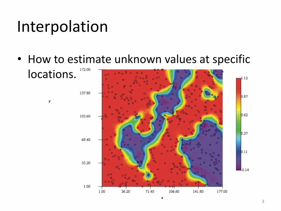
Interpolation
• How to estimate unknown values at specific locations.
3
Spatial Interpolation
• Examples
– Trend surfaces
– Nearest neighbours: Thiessen(voronoi)
– Inverse distance weighting (IDW)
– Splines
– Kriging
4

Example: Site x y z D to
(5,5)
1 2 2 3 4.2426
2 3 7 4 2.8284
3 9 9 2 5.6569
4 6 5 4 1.0000
5 5 3 6 2.0000
3
4
2
4
6
0
2
4
6
8
10
0 2 4 6 8 10
We would like to estimate the variable value at (5,5)
5

Example: IDW
• Value of z(x) is estimated from all known values of z at all n points. (Weighted Moving Average technique)
Weights usually add to 1,
n
i
iizwxz1
)(
6
n
i
iw1
1
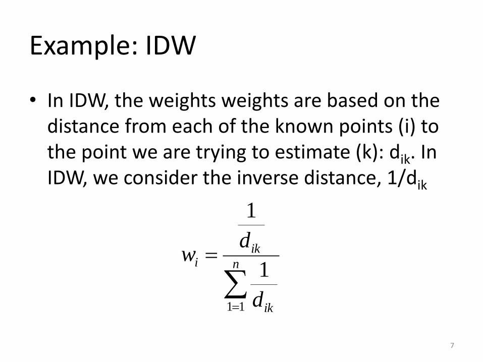
Example: IDW
• In IDW, the weights weights are based on the distance from each of the known points (i) to the point we are trying to estimate (k): dik. In IDW, we consider the inverse distance, 1/dik
7
n
ik
iki
d
dw
11
1
1
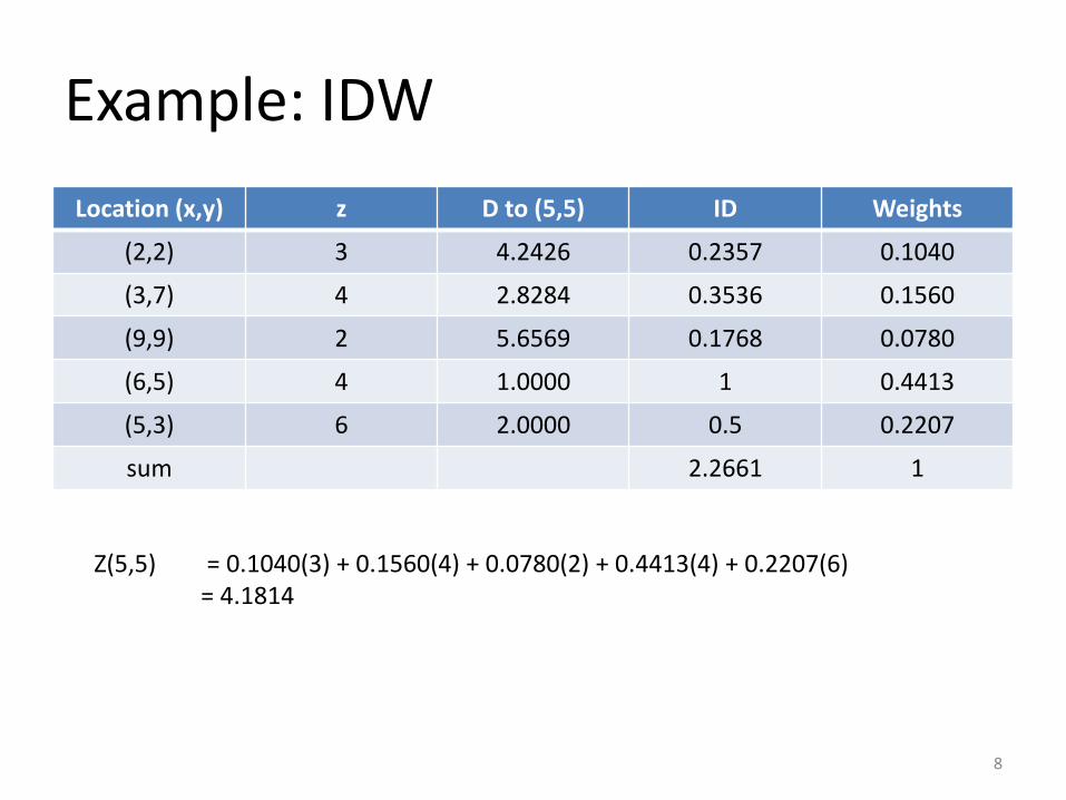
Example: IDW
Location (x,y) z D to (5,5) ID Weights
(2,2) 3 4.2426 0.2357 0.1040
(3,7) 4 2.8284 0.3536 0.1560
(9,9) 2 5.6569 0.1768 0.0780
(6,5) 4 1.0000 1 0.4413
(5,3) 6 2.0000 0.5 0.2207
sum 2.2661 1
8
Z(5,5) = 0.1040(3) + 0.1560(4) + 0.0780(2) + 0.4413(4) + 0.2207(6) = 4.1814

Historical background
• Geostatistics, first developed by Georges Matheron (1930-2000), the French geomathematician. The major concepts and theory were discovered during 1954-1963 while he was working with the French Geological Survey in Algeria and France.
• In 1963, he defined the linear geostatistics and concepts of variography, varaiances of estimation and kriging (named after Danie Krige) in the Traité de géostatistique appliquée. The principles of geostatistics was published in Economic Geology Vol. 58, 1246-1266.
• Kriging was named in honour of Danie Krige (1919-2013), the South African mining engineer who developed the methods of interpolation.
9

What is Geostatistics
• Techniques which are used for mapping of surfaces from limited sample data and the estimation of values at unsampled locations
• Geostatistics is used for: – spatial data modelling – characterizing the spatial variation – spatial interpolation – simulation – optimization of sampling – characterizing the uncertainty
• The idea of geostatistics is the points which are close to each other in the space should be likely close in values.
10

• Mining • Geography • Geology • Geophysics • Oceanography • Hydrography • Meterology • Biotechnology • Enviromental studies • Agriculture
11
Geostatistical methods provide
• How to deal with the limitations of deterministic interpolation
• The prediction of attribute values at unvisited points is optimal
• BLUE (Best Linear Unbiased Estimate)
12
Geostatistical method for interpolation
• Reconigtion that the spatial variation of any continuous attribute is often too irregular to be modelled by a simple mathematical function.
• The variation can be described better by a stochastic surface.
• The interpolation with geostatistics is known as kriging.
13
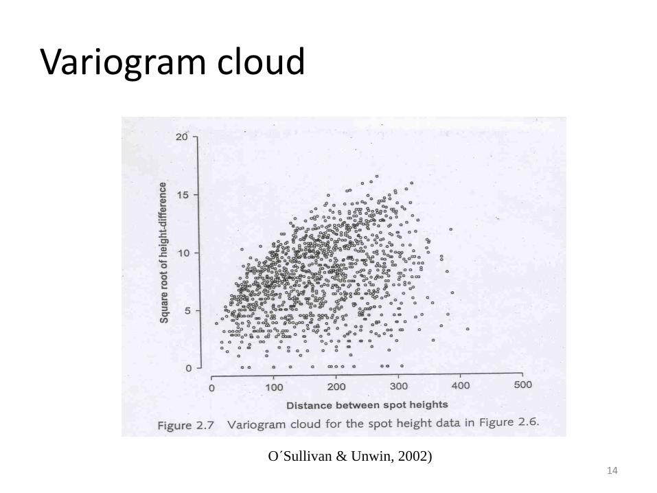
Variogram cloud
14 O´Sullivan & Unwin, 2002)
Variogram/Semivariogram
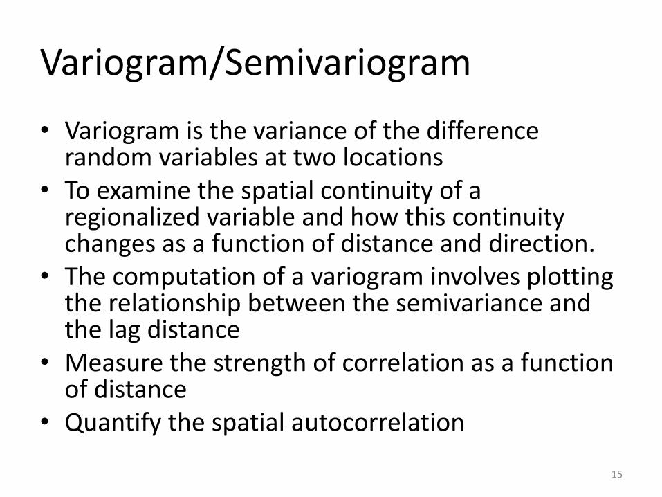
• Variogram is the variance of the difference random variables at two locations
• To examine the spatial continuity of a regionalized variable and how this continuity changes as a function of distance and direction.
• The computation of a variogram involves plotting the relationship between the semivariance and the lag distance
• Measure the strength of correlation as a function of distance
• Quantify the spatial autocorrelation
15
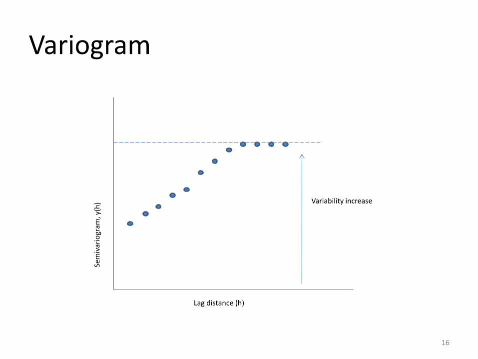
Variogram
16
Lag distance (h)
Sem
ivar
iogr
am, y
(h)
Variability increase

hhji
ji
ij
xxhN
h)|,(
2)()(2
1
Variograms
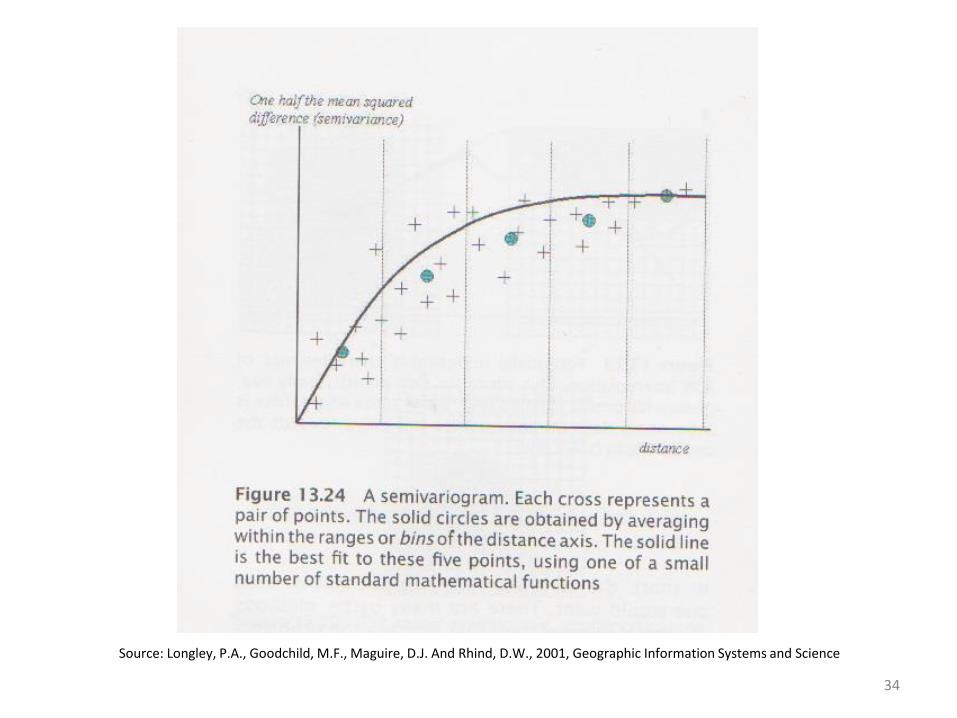
• Half of average squared difference between the paired data values.
• The variogram calculated by
17

Variogram
• Experimental variogram (sample or observed variogram) :
– when variogram is computed from sampled data.
– The first step towards a quantitative description of the regionalized variation.
• Theoretical variogram or variogram model:
– when it is modelled to fit the experimental variogram.
18
19
Omnidirectional variogram
• Omnidirectional variogram is a test for erratic directional variograms
• The omnidirectional variogram contains more sample pairs than any directional variogram so it is more likely to show a clearly interpretable structure.
• If the omnidirectional variogram is messy, then try to discover the reasons for the erraticness, e.g. Examine the h-scatterplots may reveal that a single sample value shows large influence on the calculations.
20

Isotropy
• The spatial correlation structure has no directional effects, the resulting variogram averages the variogram over all directions.
• The covariance function, correlogram, and semivariogram depend only on the magnitude of the lag vector h and not the direction
• The empirical semivariogram can be computed by pooling data pairs separated by the appropriate distances, regardless of direction.
• The semevariogram describes omnidirectional.
21

22
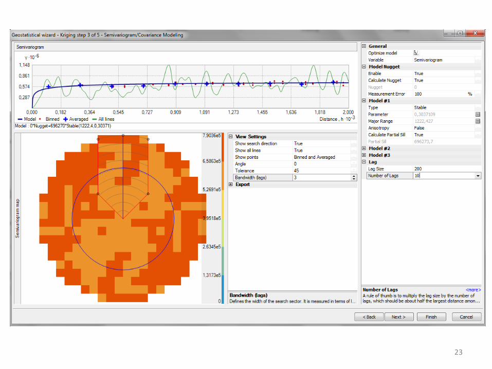
23
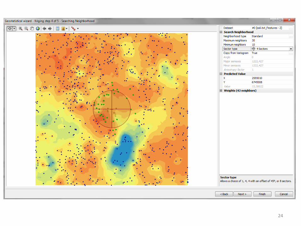
24

Anisotropy
• Spatial variation is not the same in all directions
• The variogram is computed for specific directions
• If the process is anisotropy, then so is the variogram
25
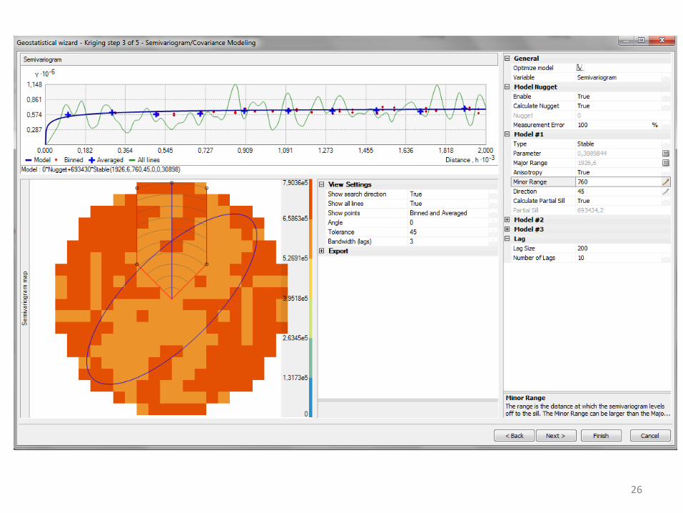
26

27
Fitting variogram models
• Why do we need a variogram model?
– We need a variogram value for some distance or direction for which we do not have a sample variogram value.
28

Fitting variogram models
• Fitting variogram models can be difficult – The accuracy of the observed semivariance is not
constant
– The variation may be anisotropic
– The experimental variogram may contain much point-to-point fluctuation
– Most models are non-linear in one or more parameters
• Both visual inspection and statistical fitting are recommended
29
Fitting variogram models
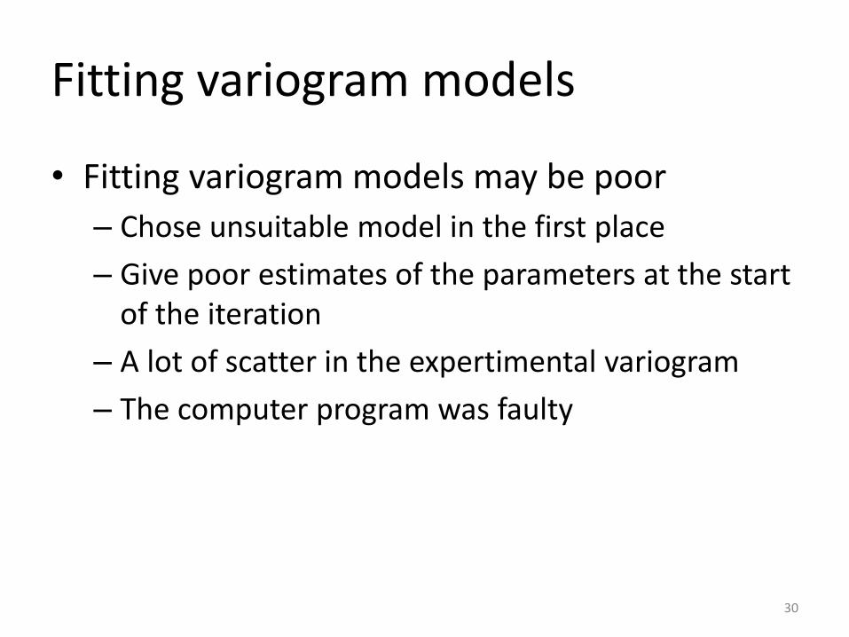
• Fitting variogram models may be poor
– Chose unsuitable model in the first place
– Give poor estimates of the parameters at the start of the iteration
– A lot of scatter in the expertimental variogram
– The computer program was faulty
30

Description
• Lag – The distance between sampling pairs. • Range – The point where the semivariogram
reaches the sill on the lag h axis. Sample points that are farther apart than range are not spatially autocorrelated.
• Nugget – The point where semivariance intercepts the ordinate.
• Sill – The value where the semivariogram first flattens off, the maximum level of semivariance. The points above the sill indicate negative spatial correlation and vice versa.
31

Fitting variogram models
32
Lag (h)
h h
h h
Lag (h)
Lag (h) Lag (h)
sill
sill
sill range range
range
nugget nugget
nugget nugget
Spherical
Gaussian Linear
Exponenial
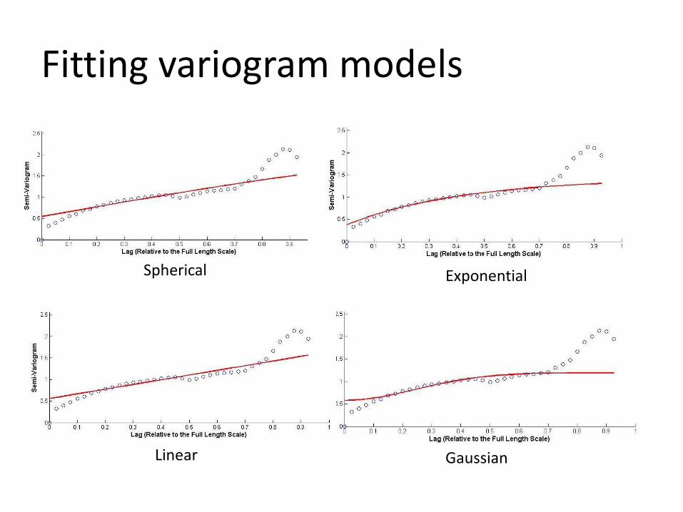
Fitting variogram models
Gaussian Linear
Spherical Exponential
34
Source: Longley, P.A., Goodchild, M.F., Maguire, D.J. And Rhind, D.W., 2001, Geographic Information Systems and Science
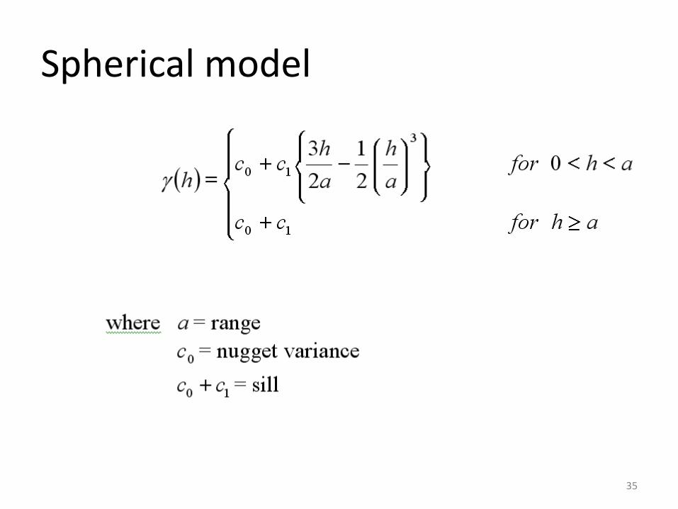
Spherical model
35
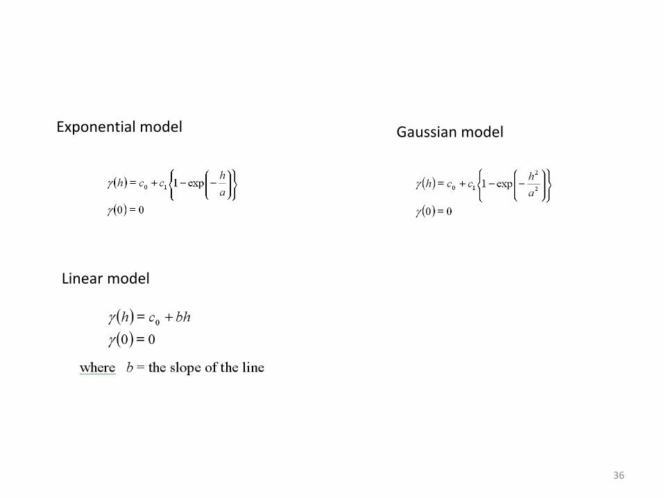
36
Exponential model
Linear model
Gaussian model

Nested structure
• One variogram model can be created by several variogram models
37
)()()(
)()(
21
1
hhh
and
hh
t
i
n
i
i
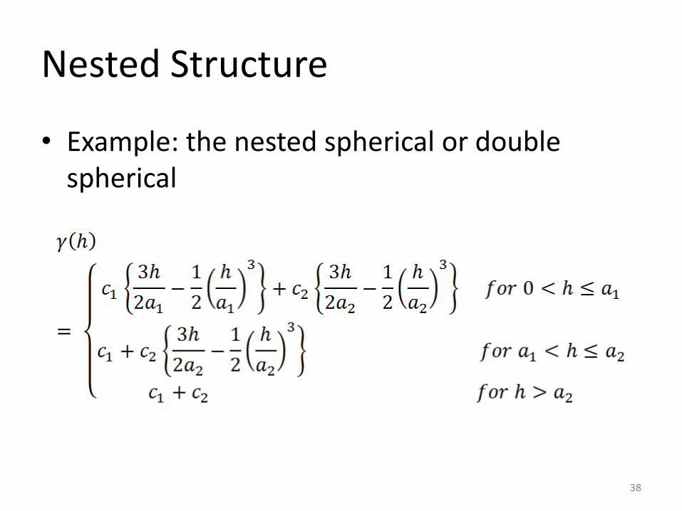
Nested Structure
• Example: the nested spherical or double spherical
38

Ordinary kriging
• In ordinary kriging, a probability model is used in which the bias and error variance can be computed and select weights for the neighbour sample locations that the everage error for the model is 0 and the error variance is minimized.
• The procedure of ordinary kriging is similar to weighted moving average except the weights are derived from geostatistical analysis.
39
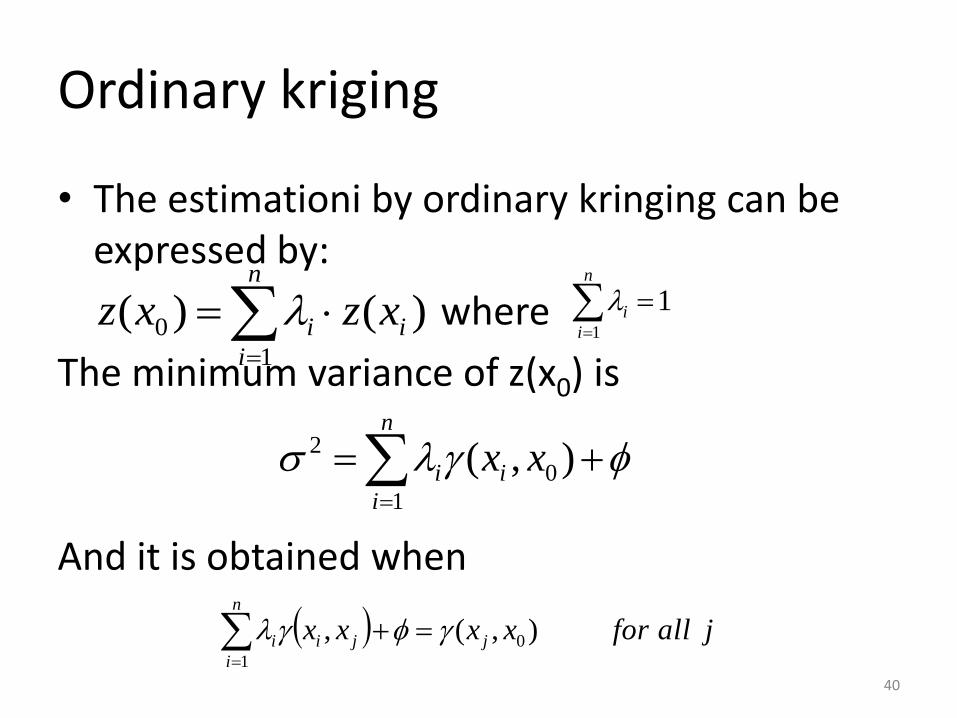
Ordinary kriging
40
• The estimationi by ordinary kringing can be expressed by:
where
The minimum variance of z(x0) is
And it is obtained when
n
i
ii xzxz1
0 )()(
n
i
i
1
1
n
i
ii xx1
0
2 ),(
n
i
jjii jallforxxxx1
0 ),(,
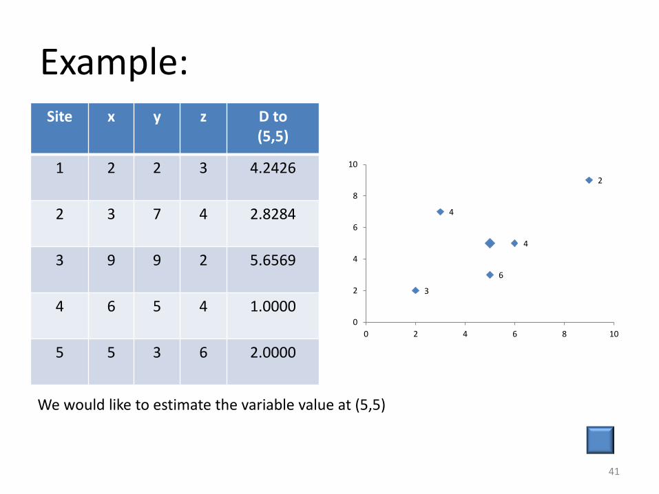
Example: Site x y z D to
(5,5)
1 2 2 3 4.2426
2 3 7 4 2.8284
3 9 9 2 5.6569
4 6 5 4 1.0000
5 5 3 6 2.0000
3
4
2
4
6
0
2
4
6
8
10
0 2 4 6 8 10
We would like to estimate the variable value at (5,5)
41
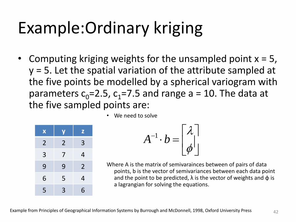
Example:Ordinary kriging
• Computing kriging weights for the unsampled point x = 5, y = 5. Let the spatial variation of the attribute sampled at the five points be modelled by a spherical variogram with parameters c0=2.5, c1=7.5 and range a = 10. The data at the five sampled points are:
• We need to solve
Where A is the matrix of semivarainces between of pairs of data points, b is the vector of semivariances between each data point and the point to be predicted, λ is the vector of weights and φ is a lagrangian for solving the equations.
x y z
2 2 3
3 7 4
9 9 2
6 5 4
5 3 6
Example from Principles of Geographical Information Systems by Burrough and McDonnell, 1998, Oxford University Press
bA 1
42
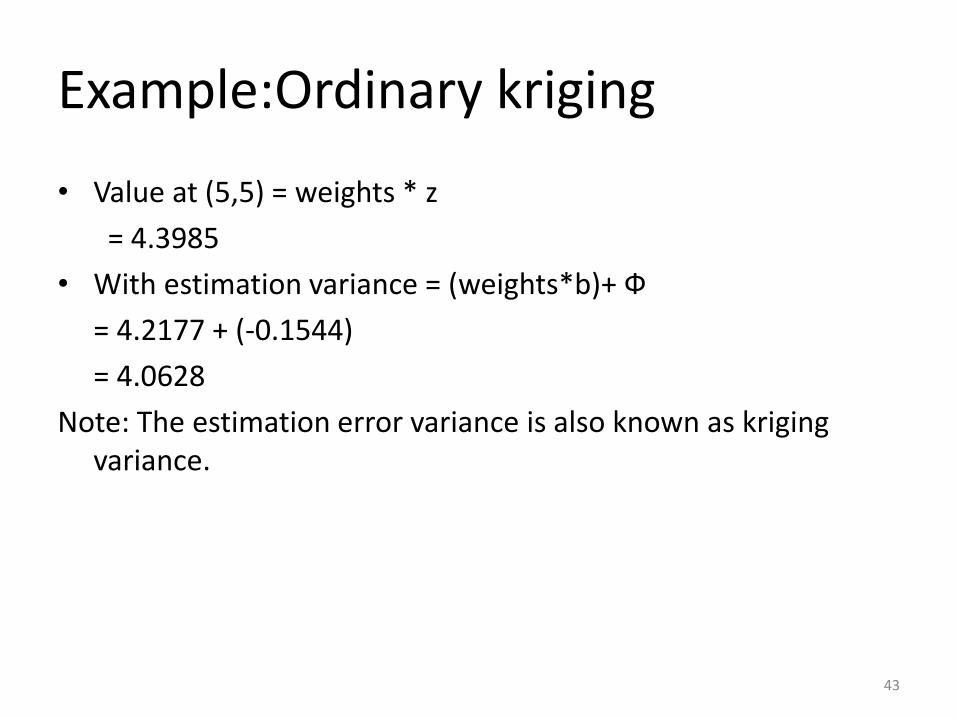
Example:Ordinary kriging
• Value at (5,5) = weights * z
= 4.3985
• With estimation variance = (weights*b)+ Ф
= 4.2177 + (-0.1544)
= 4.0628
Note: The estimation error variance is also known as kriging variance.
43

Comparison of the results
Method Estimate value z(5,5)
IDW 4.1814
Ordinary Kriging (Kriging variance)
4.3985 (4.0628)
44

Block kriging
• The modification of kriging equations to estimate an average value z(B) of the variable z over a block of area B.
z5
z4
z3
z2
z1
0
2
4
6
8
10
0 2 4 6 8 10
45

Block kriging
46
Example showing a regular 2x3 grid of point locations within a block. Each discretizing point accounts for the same area.
Example from An introduction to applied Geostatistics by Edward H. Isaaks and R.Mohan Srivastava
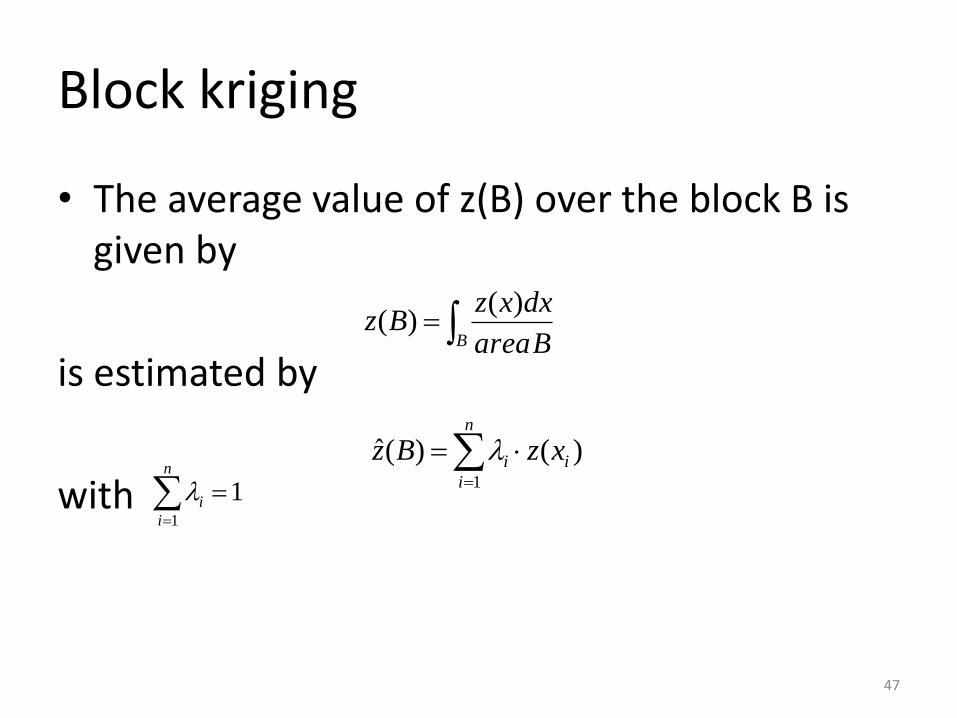
Block kriging
• The average value of z(B) over the block B is given by
is estimated by
with
B Barea
dxxzBz
)()(
n
i
ii xzBz1
)()(ˆ
n
i
i
1
1
47

Block kriging
• The minimum variance is
and is obtained with
),(),()(1
2 BBBxB i
n
i
i
n
i
jjii jallforBxxx1
),(),(
48
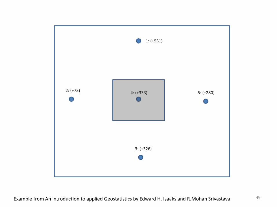
4: (+333)
1: (+531)
3: (+326)
5: (+280) 2: (+75)
Example from An introduction to applied Geostatistics by Edward H. Isaaks and R.Mohan Srivastava 49
4: (+333)
1: (+531)
3: (+326)
5: (+280) 2: (+75)
50
a
d c
b

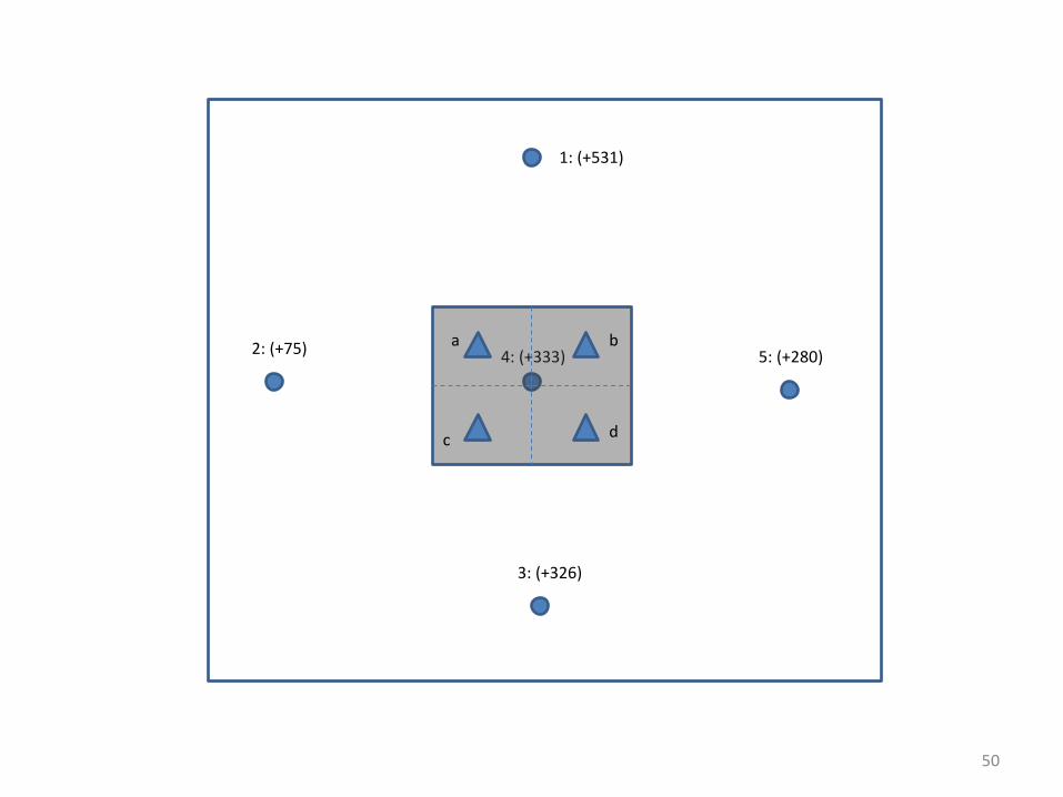
Example: Block kriging
Point Estimate Kriging weights for samples
1 2 3 4 5
a 336 0.17 0.11 0.09 0.60 0.03
b 361 0.22 0.03 0.05 0.56 0.14
c 313 0.07 0.12 0.17 0.61 0.03
d 339 0.11 0.03 0.12 0.62 0.12
Average 337 0.14 0.07 0.11 0.60 0.08
51
Simple kriging
• It is similar to ordinary kriging except that the weights sum equation (=1) is not added.
• The mean is a known constant.
• It uses the average of the entire data set. (ordinary kriging uses local average : the average of the points in the subset for a particular interpolation point)
52

Cokriging
• It is an extension of ordinary kriging where two or more variables are interdependent.
• How: • U and V are spatial correlated
• Variable U can be used to predict variable V that is information about spatial variation of U can help to map V.
– Why: • V data may be expensive to measure or collect or have some
limitations in data collection process so the data may be infrequent.
• U data, on the other hand, may be cheap to measure and possible to collect more observations.
53
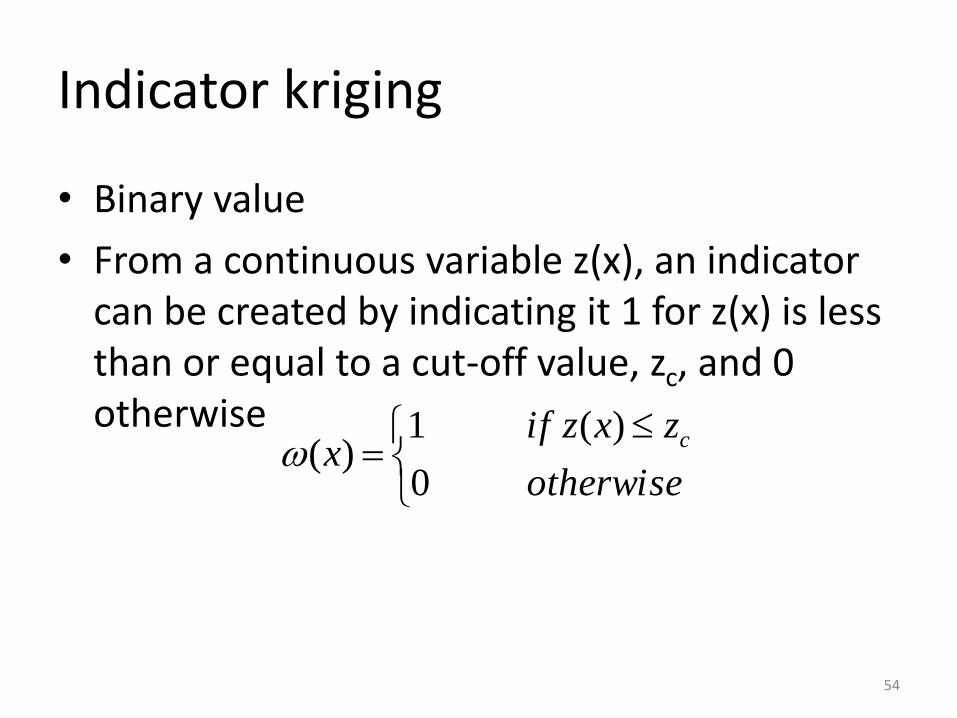
Indicator kriging
• Binary value
• From a continuous variable z(x), an indicator can be created by indicating it 1 for z(x) is less than or equal to a cut-off value, zc, and 0 otherwise
54
otherwise
zxzifx
c
0
)(1)(
Kriging: Step by step
• Studying the gathered data: data analysis
• Fitting variogram models: experimental variogram and theoretical variogram models
• Estimating values at those locations which have not been sampled (kriging) e.g. ordinary kriging, simple kriging, indicator kriging and so on
• Examining standard error which may be used to quantify confidence levels
• Kriging interpolation
55
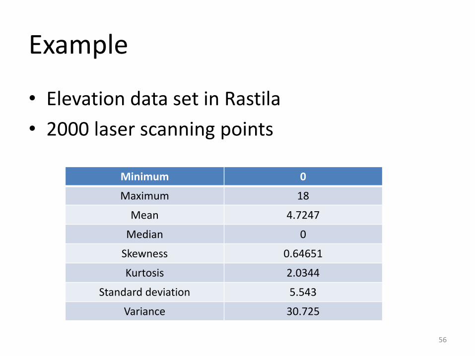
Example
• Elevation data set in Rastila
• 2000 laser scanning points
56
Minimum 0
Maximum 18
Mean 4.7247
Median 0
Skewness 0.64651
Kurtosis 2.0344
Standard deviation 5.543
Variance 30.725

Example
57

Example
58
Variogram model range nugget sill length
Exponential 0.5 0.10847 1.1232 0.18064
Linear 0.5 0.50754 1.806 -
Gaussian 0.5 0.4546 1.0447 0.22811
Spherical 0.75 0.35265 1.0666 0.48576
Exponential 0.75 0.13161 1.1388 0.19144
Linear 0.75 0.58671 1.5711 -
Gaussian 0.75 0.48089 1.0728 0.24717
Spherical 0.95 0.54285 1.9597 1.8513
Exponential 0.95 0.36872 1.4082 0.40794
Linear 0.95 0.55676 1.6424 -
Gaussian 0.95 0.57831 1.1922 0.34484

Example
59
Variogram model RMSE
Exponential (0.5) 3.281
Linear (0.5) 3.367
Gaussian (0.5) 3.431
Spherical (0.75) 3.307
Exponential (0.75) 3.272
Linear (0.75) 3.397
Gaussian (0.75) 3.439
Spherical (0.95) 3.381
Exponential (0.95) 3.302
Linear (0.95) 3.386
Gaussian (0.95) 3.466

Example
60
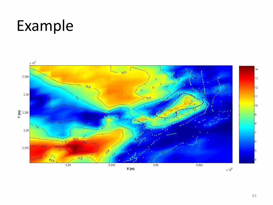
Example
61

References:
• Geographic information Analysis by Sullivan, D. And Unwin, D.
• Geostatistics for Environmental Scientists by Richard Webster and Margaret Oliver
• Principle of Geographical Information Systems, Chapter 5 and 6 by Peter Burrough and Rachael McDonnell
• An Introduction to Applied Geostatistics by Edward Isaaks and Mohan Srivastava
• Quality Aspects in Spatial Data Mining by Alfred Stein, Wenzhong Shi and Wietske Bijker
62