global agricultural reform: what is at...

decomposes the aggregate results by looking at theimpacts of partial reforms—both regionally andacross instruments—to identify what share of theglobal gains derives from reform in industrial coun-tries and what from reform in developing countriesand what share is driven by border protection andwhat by domestic support. The second set of simu-lations addresses issues raised by critics of tradereform—notably that the predicted gains for devel-oping countries are too optimistic and that the tran-sition costs for industrial-country farmers are highand too often ignored. Concerns have also beenraised about the ability of developing countries torespond to reforms and to achieve consistently highproductivity gains. To answer the questions aboutthe impacts on developing countries, three assump-tions are explored: the consequences of assumingdifferential and lower agricultural productivity insome developing countries, the impacts of con-straining output supply response in selectedlow-income countries, and estimates of trade elas-ticities. The chapter also assesses the impacts of

This chapter uses a global, dynamic applied generalequilibrium model (LINKAGE) to assess how themultifarious trade and support policies in agricul-ture affect income, trade, and output patterns at theglobal level.1 Such models have become a standardtool for assessing policy reforms because they cap-ture linkages across sectors and regions (throughtrade) and because, by their nature, they haveadding-up constraints so that supply and demandare in equilibrium in all markets. The analysis pro-vides order-of-magnitude estimates of the poten-tial consequences of policy changes, rather thana single point or “best” estimate. It also looks atthe induced structural changes, including cross-regional patterns of output and trade, which tendto be much larger than the more familiar gainsto real income. Whereas income gains typicallyamount to 1 percent of base income or less, struc-tural changes—for example, in sectoral output ortrade—can be greater than 50 percent.

Two sets of simulations are used to create adeeper picture of what drives the key results. One set

115

7

GLOBAL AGRICULTURalReform: WHAT IS

AT STAKE?

Dominique van der Mensbrugghe and John C. Beghin

With great appreciation from the authors, the underlying work in this chapter has benefited over severalyears from useful comments and suggestions from the following colleagues: Ataman Aksoy, JonathanBrooks, Bill Cline, Uri Dadush, Bernard Hoekman, Jeff Lewis, Will Martin, John Nash, Richard Newfarmer,David Roland-Holst, Josef Schmidhuber, and Hans Timmer as well as participants at seminars at the OECDand the University of California at Berkeley.

116 Global Agricultural Trade and Developing Countries

slower exit by industrial-country farmers and howthis would affect transition adjustments.

Some of the main findings:

• Reform of agricultural and food trade policyprovides 70 percent of the global gains frommerchandise trade reform—$265 billion of atotal of $385 billion.

• The global gains are shared roughly equallybetween industrial and developing countries,but developing countries gain significantly moreas a share of initial income. Significant incomegains occur in developing-country agriculture,where poverty tends to be concentrated.

• Developing countries gain more from reformingtheir own support policies than from improvedmarket access in industrial countries. Likewise,industrial countries also gain relatively morefrom their own reform.

• Notwithstanding the overall benefits fromgreater openness, structural changes are impor-tant and transition adjustments need to beaddressed.

• Productivity and supply assumptions affectimpact assessment, but their influence is small,and they do not alter the main aggregatefindings. Trade elasticities, however, are key indetermining the overall level of the incomegains. Higher elasticities dampen terms-of-tradeeffects and increase trade and real income gainsmore than proportionally, while the opposite istrue for lower elasticities. These effects can bevery large for individual countries.

The Modeling Framework

The LINKAGE model is based on a standard neo-classical general equilibrium model with firmsmaximizing profit in competitive markets and con-sumers maximizing well-being under a budget con-straint. The model has added features related to itsdynamic nature. It is global, with the world decom-posed into 23 regions, and multisectoral, witheconomic activity aggregated into 22 sectors (seeannex A in the report on the CD-ROM). Seven ofthe 23 regions are classified as high-income (orindustrial) including Canada, Western Europe(European Union-15 plus the European Free TradeAssociation countries), Japan, and the UnitedStates—the so-called Quad countries. The develop-

ing countries include some of the large countriesthat are important in agricultural markets as pro-ducers or as consumers (Argentina, Brazil, China,India, and Indonesia). The remaining developingcountries are grouped into regional aggregations.2

The sectoral decomposition is concentrated in theagricultural and food sectors (15 of the 22 sectors).

The LINKAGE model is dynamic, with scenariosspanning 1997 to 2015. The dynamics includeexogenously given labor and land growth rates,savings-driven investment and capital accumula-tion, and exogenous productivity growth. Struc-tural changes over time are driven by differentialgrowth rates and supply and demand parameters.Trade is modeled using the Armington assumption.Goods are differentiated by region of origin using atwo-nested structure (domestic absorption firstallocated across domestic and aggregate importgoods, then aggregate imports allocated acrossdifferent regions of origin).

Overview of Baseline Simulation

Assessing the impacts of policy reforms requirestwo steps in the dynamic framework of theLINKAGE model, a baseline (or reference) simula-tion and a reform simulation. The baseline involvesrunning the model forward from its 1997 base yearto 2015, with exogenous assumptions about laborand population growth rates, productivity, anddemand behavior parameters including savings,which determines the rate of capital accumulation(adjusted exogenously for depreciation).

The baseline simulation can also incorporatechanges in base year policies—to take into accountknown changes in policies (between 1997 and thepresent) or anticipated changes. The baselinedescribed below assumes no changes in base yearpolicies, however; they are held at their 1997 levels.Thus the reform simulations reflect changes fromtheir 1997 levels, not changes that would be antici-pated from 2004 levels.3 It is unclear in whichdirection some past and anticipated changes wouldaffect the global trade reform results. Some changesclearly reflect further opening—for example,China’s accession to the World Trade Organization(WTO) and some bilateral free trade agreements.Others would go in the opposite direction—forexample, the changes to the U.S. farm supportprograms.

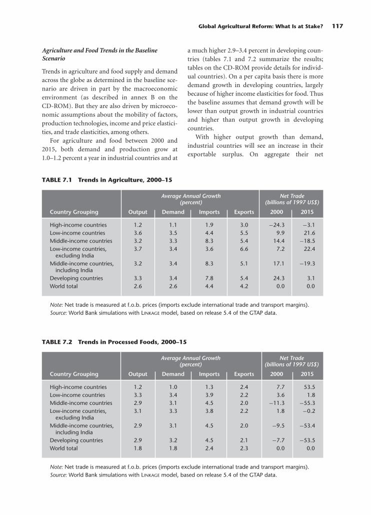
Agriculture and Food Trends in the BaselineScenario

Trends in agriculture and food supply and demandacross the globe as determined in the baseline sce-nario are driven in part by the macroeconomicenvironment (as described in annex B on theCD-ROM). But they are also driven by microeco-nomic assumptions about the mobility of factors,production technologies, income and price elastici-ties, and trade elasticities, among others.

For agriculture and food between 2000 and2015, both demand and production grow at1.0–1.2 percent a year in industrial countries and at

a much higher 2.9–3.4 percent in developing coun-tries (tables 7.1 and 7.2 summarize the results;tables on the CD-ROM provide details for individ-ual countries). On a per capita basis there is moredemand growth in developing countries, largelybecause of higher income elasticities for food. Thusthe baseline assumes that demand growth will belower than output growth in industrial countriesand higher than output growth in developingcountries.

With higher output growth than demand,industrial countries will see an increase in theirexportable surplus. On aggregate their net

Global Agricultural Reform: What Is at Stake? 117

TABLE 7.2 Trends in Processed Foods, 2000–15

Average Annual Growth Net Trade(percent) (billions of 1997 US$)

Country Grouping Output Demand Imports Exports 2000 2015

High-income countries 1.2 1.0 1.3 2.4 7.7 53.5Low-income countries 3.3 3.4 3.9 2.2 3.6 1.8Middle-income countries 2.9 3.1 4.5 2.0 −11.3 −55.3Low-income countries, 3.1 3.3 3.8 2.2 1.8 −0.2

excluding IndiaMiddle-income countries, 2.9 3.1 4.5 2.0 −9.5 −53.4

including IndiaDeveloping countries 2.9 3.2 4.5 2.1 −7.7 −53.5World total 1.8 1.8 2.4 2.3 0.0 0.0

Note: Net trade is measured at f.o.b. prices (imports exclude international trade and transport margins).Source: World Bank simulations with LINKAGE model, based on release 5.4 of the GTAP data.

TABLE 7.1 Trends in Agriculture, 2000–15

Average Annual Growth Net Trade(percent) (billions of 1997 US$)


High-income countries 1.2 1.1 1.9 3.0 −24.3 −3.1Low-income countries 3.6 3.5 4.4 5.5 9.9 21.6Middle-income countries 3.2 3.3 8.3 5.4 14.4 −18.5Low-income countries, 3.7 3.4 3.6 6.6 7.2 22.4

excluding IndiaMiddle-income countries, 3.2 3.4 8.3 5.1 17.1 −19.3

including IndiaDeveloping countries 3.3 3.4 7.8 5.4 24.3 3.1World total 2.6 2.6 4.4 4.2 0.0 0.0


agricultural and food trade will improve dramati-cally from a deficit of $17 billion in 2000 to a sur-plus of $50 billion in 2015 (at 1997 prices). Theopposite occurs in developing countries, where a netpositive balance in agriculture and food turns into alarge deficit of $50 billion, due mostly to a balloon-ing deficit in processed food. Agriculture and foodbalances are positive for low-income countries in2000 and 2015.

Developing a baseline of the future world econ-omy requires nuanced analysis. The country andregional growth rates used here are in line withconsensus views, given stronger demographictrends and income elasticities for agriculture andfood in developing economies. World and regionaltotals may be skewed by several factors. The weightsare biased toward industrial countries because ofthe use of base year (1997) value shares. Volumeshares would yield different figures. Demandgrowth in developing countries may be overstatedbecause income elasticities are held constant attheir base year levels. It is plausible to argue thatincome elasticities would converge toward those ofhigh-income countries as developing countriesgrow. The growth numbers are also broadly consis-tent with Food and Agriculture Organization(FAO) historical trends. The discrepancy betweenagricultural growth and food processing originatesin the growth in intermediate demand for agricul-tural products as food processing grows. A moremeat-intensive future world would also exhibit aslight acceleration in agricultural growth relative tofood because of the feed input in the livestocksector. So, while the baseline scenario is plausible,aggregate growth rates should be used with cautionfor all these reasons.

The biggest mover among developing countriesis China, where the food deficit of $8 billion in 1997would swell to somewhere around $120 billion by2015. Demand is expected to outpace output byabout 1 percentage point a year.4 In agriculture thisprovides new opportunities for Sub-Saharan Africaand Latin America, with both seeing a large rise inagricultural surplus (on an aggregate basis). Sub-Saharan Africa will nonetheless see a slight deterio-ration in its processed-food balance. The aggregatenet trade balances may mask more detailed sectoralshifts. For example, Sub-Saharan Africa will con-tinue to be a net importer of grains through thebaseline scenario time horizon, and therefore a rise

in world prices induced by trade reform could leadto a negative terms-of-trade shock since the agri-cultural commodities they tend to export—forexample, coffee and cocoa—already have relativelyfree access.

With relatively low demand growth in industrialcountries and relatively high output growth, theexportable agricultural surplus will increase sub-stantially, particularly from North America andOceania. Europe and Japan are the exceptions, withoutput growth expected to be anemic.

The Impacts of AgriculturalReform

The impacts of agricultural trade reform are exam-ined first in the context of global merchandise tradereform, and then the results are decomposed bytype of reform and region, to assess the relativeimportance for developing countries of reforms inindustrial countries and in developing countries.

Results of Global Merchandise Trade Reform

Global reform involves removing protection in all(nonservice) sectors, in all regions, and for allinstruments of protection (leaving other taxesunchanged, although lump-sum taxes (or trans-fers) on households adjust to maintain a fixed gov-ernment fiscal balance). The model contains sixinstruments of protection:

• Import tariffs, eliminated only if they arepositive

• Export subsidies, eliminated only if they arenegative5

• Capital subsidies, with direct payments con-verted into subsidies on capital

• Land subsidies, with some payments also con-verted to subsidies on land

• Input subsidies• Output subsidies

The overall measure of reform, referred to asreal income, measures the extent to which house-holds are better off in the post-reform scenariothan in the baseline scenario in the year 2015.6 Theworld gain (measured in 1997 U.S. dollars) is$385 billion, an increase from baseline income ofsome 0.9 percent (table 7.3). The gains are relatively


evenly divided between industrial countries($188 billion) and developing countries ($197 bil-lion), but developing countries are considerablybetter off as a share of reference income, with a gainof 1.7 percent compared with 0.6 percent for indus-trial countries.

Caveats. A few caveats about the basic globalreform scenario. First, there are known deficienciesin the base year policies, which are taken from release5.4 of the Global Trade Analysis Project (GTAP)database. Most preferential arrangements—including the Generalized System of Preferencesand some regional trading agreements—are notincorporated.7 Alternative scenarios could be under-taken to test their overall importance especiallyregarding the utilization rates of the preferences.Second, the reference scenario assumes no changesin the base year policies between the base and termi-nal years. Thus changes in trading regimes since1997, such as China’s accession to the WTO, or antic-

ipated changes, such as the elimination of the Multi-fiber Arrangement, are not taken into account.8

Third, changes to some key assumptions orspecifications could generate higher benefits. Forexample, raising the trade elasticities—as somehave argued—dampens the negative terms-of-trade effects. Increasing returns to scale can gener-ate greater efficiency improvements, dependingon the structure of product markets and scaleeconomies to be achieved. Reform of services couldhave economywide impacts to the extent thatcheaper and more efficient services can lower pro-duction costs as well as improve real incomes.Changes in investment flows—not modeled here—have proven to be as important (sometimes more)as lowering trade barriers in many regional agree-ments. In a global model, the net change would bezero. Therefore, any reallocation of capital wouldlead some countries to be better off, all else remain-ing the same, and others worse off (abstractingfrom the benefits of future repatriated profits).


TABLE 7.3 Real Income Gains and Losses from Global Merchandise Trade Reform:Change from 2015 Baseline

Export Capital Land Input OutputAll Tariffs Subsidies Subsidies Subsidies Subsidies Subsidies

Country Grouping Instruments Only Only Only Only Only Only

Change in value(billions of 1997 US$)

High-income countries 188.3 160.4 1.4 1.1 −4.8 −0.3 9.0Low-income countries 31.9 34.6 −1.1 −0.1 −0.7 −0.3 0.2Middle-income countries 164.7 187.7 −7.0 −1.2 −7.3 −3.8 −6.4Low-income countries, 19.9 21.5 −0.9 −0.1 −0.6 −0.2 0.9

excluding IndiaMiddle-income countries, 176.7 200.8 −7.3 −1.2 −7.4 −3.9 −7.0

including IndiaDeveloping countries 196.5 222.3 −8.2 −1.3 −8.1 −4.1 −6.2World total 384.8 382.7 −6.8 −0.2 −12.8 −4.4 2.8

Percentage changeHigh-income countries 0.6 0.5 0.0 0.0 0.0 0.0 0.0Low-income countries 1.6 1.7 −0.1 0.0 0.0 0.0 0.0Middle-income countries 1.8 2.0 −0.1 0.0 −0.1 0.0 −0.1Low-income countries 1.9 2.1 −0.1 0.0 −0.1 0.0 0.1

excluding IndiaMiddle-income countries 1.7 1.9 −0.1 0.0 −0.1 0.0 −0.1

including IndiaDeveloping countries 1.7 1.9 −0.1 0.0 −0.1 0.0 −0.1World total 0.9 0.9 0.0 0.0 0.0 0.0 0.0

Source: World Bank simulations with LINKAGE model, based on release 5.4 of the GTAP data.

Gross flows could have a greater impact than netcapital flows to the extent that they raise productiv-ity if they are associated with technology-ladencapital goods. Finally, dynamic effects can also leadto a boost in the overall gains from reform.

The global scenario captures some of the inher-ent dynamic gains, notably changes from savingsand investment behavior. These can sometimeshave a substantial impact, to the extent thatimported capital goods are taxed. Assuming thatsavings rates are unchanged, a sharp fall in the priceof capital goods can lead to a significant rise ininvestment (more bang per dollar invested). Thescenario does not incorporate changes to produc-tivity, however. The channels and magnitudes oftrade-related changes to productivity are as yetpoorly validated by solid empirical evidence, andattempts to incorporate these effects are by andlarge simply illustrative of potential magnitudes.Recent World Bank reports suggest that theseeffects could be large, but the reports are really anappeal for more empirical research.9

Decomposition by instrument. The key findingon instruments of protection is the predominantrole of tariffs. Removal of tariffs accounts for virtu-ally all of the gains. The other instruments havemuch smaller impacts on real income—slightlypositive on average for industrial countries andnegative in aggregate for developing countries. Forexample, elimination of export subsidies negativelyaffects Africa—both North and Sub-Saharan—andthe Middle East, although it provides a positivebenefit for Europe. Elimination of domestic protec-tion also tends to be negative for developingcountries, and at times for industrial countries aswell. The rest of Sub-Saharan Africa is a notableexception, with an income gain of 0.6 percent. Thiscould reflect the removal of significant output sub-sidies on cotton in some of the major producingcountries (China and the United States).

The ambiguity of the welfare impact is in partdriven by the nature of partial reforms. Removal ofone form of protection may exacerbate the negativeeffects of other forms of protection. For example,removal of output subsidies may worsen the impactof tariffs if removal of the subsidies leads to areduction in output and an increase in imports.There are no robust theoretical arguments to deter-mine which is more harmful. There are also other

general equilibrium effects inherent in multisec-toral global models.

While the aggregate measure of gain often gar-ners the most attention—at least from policy mak-ers and the media—more relevant for most playersare the detailed structural results. By and large, it isthe structural results that influence the politicaleconomy of reforms, particularly since the losersfrom reforms tend to be concentrated and a well-identified pressure group, whereas the gainers aretypically diffuse and harder to identify. For exam-ple, a 10 percent decline in the price of wheat couldhave a major impact on a farmer’s income, butan almost imperceptible effect on the averageconsumer.

With reform, aggregate agricultural output ofindustrial countries declines—by more than11 percent when all forms of protection are elimi-nated (table 7.4). Removal of tariff protection gen-erates the greatest change to production in indus-trial countries, but unlike the case with the welfareimpacts, the other forms of protection have meas-urable, if smaller, impacts on output. Removal ofoutput subsidies results in the next greatest changein agricultural output, driven largely by the nearly5 percent output decline in the United States—although land and export subsidies have nearly thesame aggregate impact. The detailed results for theQuad countries confirm several points of commonwisdom regarding the patterns of protection. First,the United States makes more use of output subsi-dies than do Europe and Japan. Europe makesgreater use of export subsidies and direct payments(capital and land subsidies). Japanese protection ismostly in the form of import barriers.

Results of Agricultural Reform

Full merchandise trade reform provides a bench-mark from which to judge the maximal effects fromreform. This section focuses on the agricultural andfood sectors.

Real income gains. If all regions remove all pro-tection in agriculture and food, the global gains in2015 amount to $265 billion—nearly 70 percent ofthe gains from full merchandise trade reform(table 7.5). This is remarkable considering thesmall size of agriculture and food in global output(figure 7.1).10 Agriculture represents less than



TABLE 7.4 Agricultural Output Gains and Losses from Global Merchandise Trade Reform:Change from 2015 Baseline

Export Capital Land Input OutputAll Tariffs Subsidies Subsidies Subsidies Subsidies Subsidies

Country Grouping Instruments Only Only Only Only Only Only


High-income countries −109.7 −56.2 −9.5 −1.6 −10.4 −7.4 −12.0Low-income countries 14.8 11.5 1.1 0.0 0.7 0.4 2.0Middle-income countries 41.8 18.1 8.2 −0.2 8.5 0.5 9.3Low-income countries, 13.7 10.5 0.9 0.0 0.5 0.3 2.8

excluding IndiaMiddle-income countries, 42.9 19.2 8.4 −0.2 8.7 0.6 8.6

including IndiaDeveloping countries 56.6 29.7 9.3 −0.1 9.2 0.9 11.3World total −53.1 −26.6 −0.2 −1.7 −1.2 −6.5 −0.7

Percentage changeHigh-income countries −11.1 −5.7 −1.0 −0.2 −1.1 −0.7 −1.2Low-income countries 2.4 1.8 0.2 0.0 0.1 0.1 0.3Middle-income countries 2.4 1.0 0.5 0.0 0.5 0.0 0.5Low-income countries, 4.1 3.1 0.3 0.0 0.2 0.1 0.8

excluding IndiaMiddle-income countries, 2.1 0.9 0.4 0.0 0.4 0.0 0.4

including IndiaDeveloping countries 2.4 1.2 0.4 0.0 0.4 0.0 0.5World total −1.6 −0.8 0.0 −0.1 0.0 −0.2 0.0


TABLE 7.5 Real Income Gains from Agricultural and Food Trade Reform: Changefrom 2015 Baseline(billions of 1997 US$)

Agricultural andGlobal Food Trade Agricultural

Merchandise Reform Trade ReformTrade Reform High-Income Only

Country Grouping Global Global Countries High-Income

High-income countries 188.3 136.6 92.0 29.3Low-income countries 31.9 10.3 3.0 1.1Middle-income countries 164.7 118.2 6.9 −4.9Low-income countries, 19.9 8.4 3.6 1.6

excluding IndiaMiddle-income countries, 176.7 120.1 6.4 −5.3

including IndiaDeveloping countries 196.5 128.6 10.0 −3.8World total 384.8 265.2 102.0 25.5


2 percent of output for industrial countries and10.5 percent for developing countries, whileprocessed foods represent 4.5 percent for industrialcountries and 7.5 percent for developing countries.Agriculture is still a relatively high 19 percent ofoutput in the low-income developing countries.Clearly, protection tends to be higher in agricultureand food than in other sectors, particularly inindustrial countries, but in middle-income coun-tries as well. Protection is more uniform in low-income countries.

For low-income countries the gains from globalfree trade in agriculture and food amount toaround one-third of the gains from global freetrade in all merchandise. This is a consequence oftheir dependence on imports of the most protectedfood items—such as grains—while they are netexporters of commodities with little or no protec-tion. The middle-income countries gain 71 percentfrom global free trade in agriculture and food,nearly as much as industrial countries, which gain72 percent as compared with full merchandisetrade reform.

If reforms are limited to high-incomecountries—a super-version of special and differen-tial treatment—with perhaps an agreement bymiddle-income countries to bind at existing levelsof protection, global gains drop to $102 billion,indicating that a significant portion of the globalgains is generated by removal of agricultural barri-ers in developing countries (see table 7.5).11 Thedrop in gains is particularly striking for middle-

income countries, where the gains from their ownagricultural and food reform would be quite sub-stantial. On a percentage basis, this is less so forlow-income countries. The industrial countriesreap gains of $92 billion, implying that agriculturalreform in developing countries could generategains of about $45 billion for the industrialcountries.

The final decomposition scenario is to assess theimpacts of reform in agriculture alone in industrialcountries—leaving protection unchanged forprocessed foods. This lowers the gains substantiallyfor industrial countries—from $92 billion to $29billion (see table 7.5). Protection is high in bothsectors, and the processed foods sector is more thantwice as large as the agricultural sector. Further-more, in a partial reform scenario, the efficiencygains in agriculture could be offset to some extentby further losses in processed foods. Output willexpand in the processed food sector as resourcesare moved around—and the lower costs of inputswill also provide incentives to increase output.Middle-income countries could lose from anagriculture-only reform in industrial countries.They would benefit little from improved marketaccess in agriculture, and in a partial reform sce-nario, expansion of their protected domestic agri-culture and food production leads to efficiencylosses that are not compensated elsewhere.

To conclude—global agricultural trade reformgenerates a huge share of the gains to be made frommerchandise trade reform. Market access into


FIGURE 7.1 Output Structure in Base Year, 1997

0

2010

30

50

70

90

40

60

80

100

Percent

Industrial Low-income Middle-income

Other goods and servicesProcessed foodsAgriculture

Manufacturing

Source: GTAP release 5.4.

industrial countries provides significant gains, buta greater share of the gains for developing countriescomes from agricultural trade reform amongdeveloping countries. Finally, reform in agriculturealone provides few benefits. It needs to be linked toreform in the processed food sectors.

Structural implications. Accelerating integrationis one of the key goals of trade reform. Beyond theefficiency gains that come from allocating resourcesto their best uses, integration is expected to bringproductivity increases—scale economies, greatercompetitiveness, ability to import technology-laden intermediate goods and capital, greater mar-ket awareness, and access to networks.

The potential changes in trade from globalreform of agriculture and food are large. Worldtrade in these two sectors could jump by more thanhalf a trillion dollars in 2015 (compared with thebaseline), an increase of 74 percent (table 7.6).

Exports in agriculture and food from developingcountries would jump $300 billion, an increase ofmore than 115 percent, with industrial-countryexports increasing $220 billion, or 50 percent. Onthe flip side, imports from both industrial anddeveloping countries would rise substantially. Thenet trade position of industrial countries woulddeteriorate marginally—from $50 billion in thebaseline in 2015 to $48 billion after global reformof agriculture and food. The marginal improve-ment for developing countries decomposes into aboost of nearly $12 billion for low-income coun-tries and deterioration for middle-income coun-tries of nearly $10 billion.

If the reform is limited to industrial countries,the picture is modified significantly. First, thechange in imports for industrial countries is almostidentical under the two scenarios—$223 billionwith full reform and $205 billion with industrial-country reform only (see table 7.6). Developing


TABLE 7.6 Impact of Global Agricultural and Food Reform on Agricultural andFood Trade: Change from 2015 Baseline

Exports Imports Net Trade

Country Grouping Global Industrial Global Industrial Global Industrial 2015 Baseline


High-income countries 221.2 63.4 223.3 205.3 −2.1 −141.9 50.4Low-income countries 41.0 20.9 29.2 −0.3 11.8 21.2 23.4Middle-income countries 260.1 120.5 269.8 −0.2 −9.7 120.7 −73.8Low-income countries, 33.8 17.5 21.9 0.1 11.8 17.5 22.2

excluding IndiaMiddle-income countries, 267.3 123.9 277.1 −0.5 −9.8 124.4 −72.7

including IndiaDeveloping countries 301.1 141.4 299.0 −0.4 2.1 141.9 −50.4World total 522.3 204.9 522.3 204.9 0.0 0.0 0

Percentage changeHigh-income countries 50 14 57 52Low-income countries 74 38 92 −1Middle-income countries 125 58 96 0Low-income countries, 70 36 84 0

excluding IndiaMiddle-income countries, 125 58 96 0

including IndiaDeveloping countries 115 54 95 0World total 74 29 74 29

Note: The columns labeled Global refer to the impacts from global agriculture and food reform.The columns labeled Industrial refer to industrial-country only reform of agriculture and food.Source: World Bank simulations with Linkage model, based on release 5.4 of the GTAP data.

countries see a significant rise in exports, but toindustrial countries only, with little or no change intheir own imports. Thus industrial countries wouldwitness a much sharper deterioration in their netfood bill, with net imports registering a change of$142 billion instead of $2 billion, as under theglobal reform scenario. The United States andEurope bear the brunt of the adjustment, withCanada, Australia, and New Zealand seeing littledifference between the global and partial reformscenarios. In other words, these three countriesreap much of the trade benefits from greater mar-ket access within industrial countries. Opening upof markets in developing countries significantlydampens the adjustment process for the UnitedStates and Europe, and the United States wouldreinforce its net exporting status significantlyunder a global reform scenario.

Most developing countries see a greater im-provement in their net food trade with industrial-country-only reform than with global reform—but not all countries. Argentina, Brazil, and the restof East Asia improve their net food trade morewith global reform than with partial reform. They

would gain additional market access from develop-ing countries and reinforce their comparativeadvantage over more highly protected countries inEast Asia. The biggest beneficiary in net termswould be China. While its (small) exports wouldnot change much, removal of its own protectioninduces a huge shift in imports. The lack of reformunder the partial reform scenario means thatinstead of its net food position deteriorating by$74 billion in the global reform, it sees a smallimprovement of $6 billion. On aggregate for devel-oping countries the partial reform would gener-ate an improvement in net trade of food of$142 billion.

The structural impacts described above are asso-ciated with global changes in the distribution offarm income. With global agriculture and foodreform, farm incomes barely change at the globallevel (a loss of perhaps $10 billion,12 or 0.6 percentof baseline 2015 farm income). Changes are muchmore significant at the regional level (figures 7.2and 7.3). The largest absolute gains in farm incomeare in the Americas, Australia and New Zealand,and developing East Asia excluding China. Latin


FIGURE 7.2 Change in Rural Value Added from Baseline in 2015(billions of 1997 $US)

�100 �80 �60 �40 �20 200 40

ChinaWestern Europe

JapanKorea, Rep. of, and Taiwan (China)

Rest of South AsiaIndia

Rest of Europe and Central AsiaRest of the world

VietnamSouthern African Customs Union

EU accession countriesIndonesia

TurkeyMexico

CanadaRest of Sub-Saharan Africa

Rest of East AsiaAustralia and New Zealand

BrazilArgentina

Rest of Latin AmericaUnited States

Source: World Bank simulations with Linkage model, based on release 5.4 of the GTAP data.

America would receive 40 percent of the total posi-tive gains; Australia, Canada, and New Zealand18 percent, and the United States 15 percent.

The relative position of regional gainers is some-what different, however (see figure 7.3). Farmers inAustralia, Canada, and New Zealand gain the mostfrom global free trade in agriculture and food, withincome gains of 50–65 percent. Farmers in a num-ber of developing regions have gains of more than25 percent—Vietnam, Argentina, countries of theSouthern Africa Customs Union (SACU), the restof East Asia (which includes Thailand, Malaysia,and the Philippines), and the rest of Latin America.

The farmers who lose most are in China, withpotential losses of $75 billion in 2015 comparedwith the baseline scenario.13 The next biggest losersare farmers in Western Europe and the developedEast Asian economies—Japan, the Republic ofKorea, and Taiwan (China). In percentage terms thebiggest losses occur in Japan (30 percent) and West-ern Europe (24 percent), with China’s losses downto about 15 percent because of its huge ruraleconomy.

Most of the impact on rural incomes is gener-ated by volume changes, not factor returns. Both

labor and capital returns are determined essentiallyon national markets.14 Thus wage changes aremodest overall, with generally greater impactsin developing countries, where more labor isemployed in agriculture (table 7.7). For example,wages for unskilled labor increase 8 percent inArgentina and Vietnam, and 5–6 percent in the restof Latin America and the rest of Sub-SaharanAfrica. Unskilled workers in Australia and NewZealand also benefit from these reforms. Unskilledworkers in developing countries generally do betterin relative terms than skilled workers, largely as aresult of their concentration in agricultural sectors.China is a significant exception. Removal of itsagricultural protection lowers demand forunskilled workers, and their wages decline. Theimpact on wages in the European Union and Japanis negligible, as agriculture employs a very smallshare of the national labor force.

As in the labor markets, the returns in capitalmarket are determined mainly at the national level(table 7.8). Thus changes to income will largely bereflected in volume changes, not price changes.Direct payments to farmers, however, are imple-mented as an ad valorem subsidy on capital (and


FIGURE 7.3 Percentage Change in Rural Value Added from Baseline in 2015

�40 �20 0 20 40 60 80

JapanWestern Europe

Korea, Rep. of, and Taiwan (China)China

Rest of South AsiaIndia

Rest of Europe and Central AsiaRest of the world

IndonesiaMexicoTurkey

EU accession countriesUnited States

BrazilRest of Sub-Saharan Africa

Rest of Latin AmericaRest of East Asia

Southern African Customs UnionArgentina

VietnamCanada

Australia and New Zealand


land), thus creating a wedge between the cost tofarmers and the returns to owners. Removal of thecapital subsidy has little effect on owners since thereturn is determined at the economywide level, butit raises the costs to farmers. For example, the costof capital net of subsidies increases by almost 1 per-cent in the European Union, but the average cost tofarmers increases by 22 percent—and even morefor livestock producers (43 percent). Note thatthese capital subsidies are used mainly in industrialcountries, so for most developing countries there isno difference between the owner return and thecost to farmers.

The changes in the contribution of land to agri-cultural incomes are driven largely by pricemovements—contrary to the case for labor andcapital income (table 7.9). Land is essentially a

fixed factor in agriculture, with some allowance formovements up and down the supply curve and forcross-sectoral shifts in land usage.15 In Europe theaverage return to land drops 66 percent, with thesupply of land falling 9 percent following globalreform. Farmers gain some benefit in lower unitcosts because of falling land prices. But removal ofthe direct subsidy does not allow farmers to reapthe full cost gains from falling land prices. Theaverage cost for farmers drops 57 percent, lowerthan the drop in the rental price of land (66 per-cent). And the change in the cost structure ishighly sector specific. Thus cereal and grain farm-ers see a small drop in their net cost of land (5 per-cent); however, the drop in the price of land doesnot compensate for removal of the subsidies sincethe returns to owners falls by 74 percent. This is


TABLE 7.7 Impact of Global Agriculture and Food Reform on Agricultural Employmentand Wages: Change from 2015 Baseline(percent)

Total Agriculture Cereals and Sugar Livestock and Dairy

Wages Wages WagesEmploy- Employ- Employ-

Country or Region ment Unskilled Skilled ment Unskilled Skilled ment Unskilled Skilled

Canada 8.5 1.0 0.8 30.4 1.0 0.8 −15.5 1.0 0.8United States 0.4 0.6 0.6 −12.4 0.6 0.6 3.3 0.6 0.6European Union −23.7 −0.6 0.4 −57.7 −0.6 0.4 −28.0 −0.6 0.4

with EFTA*Australia and 18.2 3.4 2.3 25.6 3.4 2.3 31.1 3.4 2.3

New ZealandJapan −26.8 −0.9 −0.1 −28.9 −0.9 −0.1 −46.2 −0.9 −0.1Korea, Rep. of and −13.8 −0.2 0.7 −3.9 −0.2 0.7 8.2 −0.2 0.7

Taiwan (China)Argentina 13.3 7.9 5.5 25.8 7.9 5.5 14.3 7.9 5.5Brazil 12.5 3.4 3.0 25.8 3.4 3.0 11.7 3.4 3.0China −6.6 −3.1 0.0 −26.6 −3.1 0.0 8.6 −3.1 0.0India −0.3 0.0 0.2 0.7 0.0 0.2 1.1 0.0 0.2Indonesia 4.3 1.4 −0.3 6.1 1.4 −0.3 −2.0 1.4 −0.3Mexico 5.0 1.3 −0.2 1.3 1.3 −0.2 −4.8 1.3 −0.2Southern African 13.8 1.3 1.1 31.7 1.3 1.1 8.8 1.3 1.1

Customs UnionTurkey 5.2 3.0 0.5 −15.3 3.0 0.5 −18.7 3.0 0.5Vietnam 17.0 7.8 3.0 63.1 7.8 3.0 −15.4 7.8 3.0Rest of East Asia 11.6 2.7 0.9 72.0 2.7 0.9 −9.1 2.7 0.9Rest of South Asia −1.3 −0.2 0.0 1.1 −0.2 0.0 0.7 −0.2 0.0EU accession countries 6.9 1.6 0.9 12.8 1.6 0.9 13.3 1.6 0.9Rest of Europe and −0.4 −1.0 −0.3 0.3 −1.0 −0.3 −2.4 −1.0 −0.3

Central AsiaRest of Sub-Saharan 6.2 6.0 1.9 17.9 6.0 1.9 1.2 6.0 1.9

AfricaRest of Latin America 6.2 5.4 3.4 17.9 5.4 3.4 42.6 5.4 3.4Rest of the World −0.1 −0.3 0.9 2.6 −0.3 0.9 −4.2 −0.3 0.9

including Middle East and North Africa

*European Free Trade Association, (Austria, Finland, Iceland, Norway, Sweden, and Switzerland).Source: World Bank simulations with LINKAGE model, based on release 5.4 of the GTAP data.

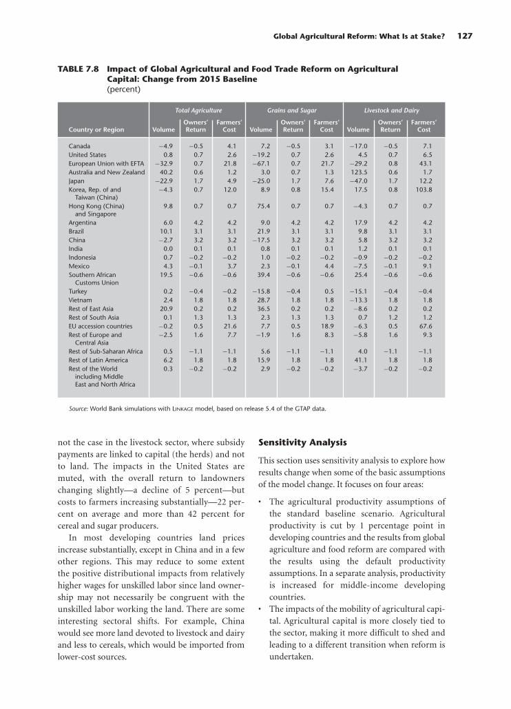
not the case in the livestock sector, where subsidypayments are linked to capital (the herds) and notto land. The impacts in the United States aremuted, with the overall return to landownerschanging slightly—a decline of 5 percent—butcosts to farmers increasing substantially—22 per-cent on average and more than 42 percent forcereal and sugar producers.

In most developing countries land pricesincrease substantially, except in China and in a fewother regions. This may reduce to some extentthe positive distributional impacts from relativelyhigher wages for unskilled labor since land owner-ship may not necessarily be congruent with theunskilled labor working the land. There are someinteresting sectoral shifts. For example, Chinawould see more land devoted to livestock and dairyand less to cereals, which would be imported fromlower-cost sources.

Sensitivity Analysis

This section uses sensitivity analysis to explore howresults change when some of the basic assumptionsof the model change. It focuses on four areas:

• The agricultural productivity assumptions ofthe standard baseline scenario. Agriculturalproductivity is cut by 1 percentage point indeveloping countries and the results from globalagriculture and food reform are compared withthe results using the default productivityassumptions. In a separate analysis, productivityis increased for middle-income developingcountries.

• The impacts of the mobility of agricultural capi-tal. Agricultural capital is more closely tied tothe sector, making it more difficult to shed andleading to a different transition when reform isundertaken.


TABLE 7.8 Impact of Global Agricultural and Food Trade Reform on AgriculturalCapital: Change from 2015 Baseline(percent)

Total Agriculture Grains and Sugar Livestock and Dairy

Owners’ Farmers’ Owners’ Farmers’ Owners’ Farmers’Country or Region Volume Return Cost Volume Return Cost Volume Return Cost

Canada −4.9 −0.5 4.1 7.2 −0.5 3.1 −17.0 −0.5 7.1United States 0.8 0.7 2.6 −19.2 0.7 2.6 4.5 0.7 6.5European Union with EFTA −32.9 0.7 21.8 −67.1 0.7 21.7 −29.2 0.8 43.1Australia and New Zealand 40.2 0.6 1.2 3.0 0.7 1.3 123.5 0.6 1.7Japan −22.9 1.7 4.9 −25.0 1.7 7.6 −47.0 1.7 12.2Korea, Rep. of and −4.3 0.7 12.0 8.9 0.8 15.4 17.5 0.8 103.8

Taiwan (China)Hong Kong (China) 9.8 0.7 0.7 75.4 0.7 0.7 −4.3 0.7 0.7

and SingaporeArgentina 6.0 4.2 4.2 9.0 4.2 4.2 17.9 4.2 4.2Brazil 10.1 3.1 3.1 21.9 3.1 3.1 9.8 3.1 3.1China −2.7 3.2 3.2 −17.5 3.2 3.2 5.8 3.2 3.2India 0.0 0.1 0.1 0.8 0.1 0.1 1.2 0.1 0.1Indonesia 0.7 −0.2 −0.2 1.0 −0.2 −0.2 −0.9 −0.2 −0.2Mexico 4.3 −0.1 3.7 2.3 −0.1 4.4 −7.5 −0.1 9.1Southern African 19.5 −0.6 −0.6 39.4 −0.6 −0.6 25.4 −0.6 −0.6

Customs UnionTurkey 0.2 −0.4 −0.2 −15.8 −0.4 0.5 −15.1 −0.4 −0.4Vietnam 2.4 1.8 1.8 28.7 1.8 1.8 −13.3 1.8 1.8Rest of East Asia 20.9 0.2 0.2 36.5 0.2 0.2 −8.6 0.2 0.2Rest of South Asia 0.1 1.3 1.3 2.3 1.3 1.3 0.7 1.2 1.2EU accession countries −0.2 0.5 21.6 7.7 0.5 18.9 −6.3 0.5 67.6Rest of Europe and −2.5 1.6 7.7 −1.9 1.6 8.3 −5.8 1.6 9.3

Central AsiaRest of Sub-Saharan Africa 0.5 −1.1 −1.1 5.6 −1.1 −1.1 4.0 −1.1 −1.1Rest of Latin America 6.2 1.8 1.8 15.9 1.8 1.8 41.1 1.8 1.8Rest of the World 0.3 −0.2 −0.2 2.9 −0.2 −0.2 −3.7 −0.2 −0.2



• Sensitivity of the results to supply rigidities indeveloping countries.

• Sensitivity of the results to the key tradeelasticities.

Agricultural Productivity

Agricultural productivity is assumed to grow2.5 percent a year globally in the standard baselinescenario based on existing evidence (Martin andMitra 1996, 1999). This may be too optimistic fordeveloping countries, particularly for low-incomecountries. This assumption may have an impact onlong-term self-sufficiency rates, particularly of sen-sitive commodities. The more trade reform raisesthe world price of food, the more net foodimporters will be adversely affected by negativeterms-of-trade shocks. To test the sensitivity of thetrade results to agricultural productivity, a different

baseline was constructed with agricultural produc-tivity improving at a slower 1.5 percent for devel-oping countries, but remaining at 2.5 percent forindustrial countries.

Trade impact. Under the standard baseline, high-income countries go from a position of net foodimporters in 1997 to net food exporters in 2015(table 7.10). Low-income countries improve theirposition significantly, going from a positive foodbalance of $12.5 billion in 1997 to $23 billion in2015. The position of middle-income countriesdeteriorates, however. Under the low-productivitybaseline, the net food trade position of industrialcountries increases substantially—jumping to $151billion in 2015 compared with only $50 billion inthe standard baseline. Low-income countries stillmaintain a positive balance, but the balance ismuch closer to zero than it was in the previous


TABLE 7.9 Impact of Global Agriculture and Food Reform on Agricultural Land:Change from 2015 Baseline(percent)

Total Agriculture Cereals and Sugar Livestock and Dairy

Price Price Price

Country or Region Land Owner Farmer Land Owner Farmer Land Owner Farmer

Canada −6.4 69.5 133.8 6.6 76.9 192.8 −25.2 56.8 83.5United States 2.4 −5.1 22.1 −19.0 −12.5 42.1 12.3 −0.2 9.1European Union with EFTA −9.4 −66.3 −57.0 −58.9 −74.1 −4.7 −3.5 −65.0 −59.7Australia and New Zealand 6.2 197.8 219.1 1.9 197.0 224.0 34.8 219.6 252.4Japan −21.0 −44.9 −41.5 −24.0 −45.5 −34.6 −34.1 −48.9 −48.9Korea, Rep. of and −11.4 −27.6 −27.1 −0.2 −25.3 −24.6 4.1 −23.0 −20.9

Taiwan (China)Argentina 4.5 56.2 56.2 11.4 59.5 59.5 12.0 60.0 60.0Brazil 9.9 18.0 18.0 23.8 22.9 22.9 8.6 17.6 17.6China −0.9 −25.7 −25.7 −21.1 −31.1 −31.1 7.6 −23.6 −23.6India 0.0 −1.8 −1.8 0.8 −1.5 −1.5 1.4 −1.3 −1.3Indonesia 0.7 10.9 10.9 2.1 11.4 11.4 −1.8 10.0 10.0Mexico 2.7 0.6 13.1 −8.9 −3.6 52.1 −1.6 −0.6 0.8Southern African 8.0 86.4 86.4 26.4 95.2 95.2 4.5 84.9 84.9

Customs UnionTurkey 0.8 47.3 47.3 −14.9 39.0 39.0 −20.2 36.1 36.1Vietnam −0.3 44.6 44.6 33.2 60.3 60.3 −16.0 38.1 38.1Rest of East Asia −1.5 34.1 34.1 43.7 53.8 53.8 −9.6 32.7 32.7Rest of South Asia −0.1 −6.0 −6.0 3.2 −5.0 −5.0 1.3 −5.4 −5.4EU accession countries 2.6 2.0 6.1 4.6 2.8 10.8 7.5 3.5 8.8Rest of Europe and −1.5 −2.4 −2.4 −1.1 −2.3 −2.3 −1.2 −2.2 −2.2

Central AsiaRest of Sub-Saharan Africa −0.3 62.8 62.8 9.0 67.9 67.9 −2.4 61.7 61.7Rest of Latin America 1.0 55.4 55.4 5.0 58.6 58.6 40.3 74.9 74.9Rest of the World 0.0 0.1 0.1 2.7 0.8 0.8 −4.3 −1.2 −1.2



baseline. And the net food trade situation ofmiddle-income countries shows a greater depend-ence on world markets.

Whereas reform in the standard baseline posi-tions low-income countries as net food exportersand has only a mild negative effect on the food bal-ance of high- and middle-income countries, underthe low-productivity assumption, the food tradebalance of the high-income countries improvessubstantially—by $30 billion—largely because ofan increased dependence on food imports bymiddle-income countries. The low-income coun-tries still see an improvement in their trade balance,

but by a more modest $3.6 billion rather than thenearly $12 billion using the standard productivityassumptions.

Output impact. Average annual agricultural out-put growth in developing countries slows from3.3 percent in the standard baseline to 2.6 percentin the low-productivity baseline (table 7.11). Inindustrial countries higher productivity providesan opportunity to gain market share, and higherworld prices relative to the original baseline pro-vide greater incentives to produce. World outputunder the alternative scenario declines 3.4 percent


TABLE 7.10 Net Trade Impacts Assuming Lower Agricultural Productivity in Developing Countries(billions of 1997 US$)

Standard Productivity Low Productivity

Baseline Reform Baseline ReformCountry Grouping 1997 2015 2015 2015 2015

High-income countries −23.1 50.4 48.4 151.2 181.6Low-income countries 12.5 23.4 35.2 0.9 4.5Middle-income countries 10.5 −73.8 −83.6 −152.0 −186.1Low-income countries, 7.4 22.2 34.1 8.5 17.2

excluding IndiaMiddle-income countries, 15.6 −72.7 −82.4 −159.7 −198.9

including IndiaDeveloping countries 23.1 −50.4 −48.4 −151.2 −181.6


TABLE 7.11 Impacts on Output Assuming Lower Agricultural Productivity forDeveloping Countries

Growth in 2000– Baseline Difference Difference between Baseline15 (percent) in 2015 and Reform Scenario in 2015

Low Standard Value Percentage Low Standard Low StandardCountry Grouping Baseline Baseline ($ billions) Change ($ billions) ($ billions) (percent) (percent)

High-income countries 1.9 1.2 122.6 12.4 −100.0 −107.7 −9.0 −10.9

Low-income countries 2.8 3.6 −71.6 −11.4 8.7 12.1 1.6 1.9

Middle-income 2.6 3.2 −166.2 −9.4 27.0 37.2 1.7 2.1countries

Low-income countries, 3.0 3.7 −39.4 −11.6 10.3 12.3 3.4 3.6excluding India

Middle-income 2.6 3.2 −198.4 −9.7 25.4 37.0 1.4 1.8countries, including India

Developing countries 2.6 3.3 −237.8 −10.0 35.7 49.4 1.7 2.1

World total 2.4 2.6 −115.2 −3.4 −64.3 −58.3 −2.0 −1.7


(higher prices lead to reduced demand), with areallocation between industrial and developingcountries. Industrial countries benefit from a12 percent increase in output in 2015 comparedwith the standard baseline, whereas developingcountry output is reduced by some 10 percent.

With respect to output impacts following thetrade reform scenario, the qualitative results of thedifferent baseline assumptions of agricultural pro-ductivity are identical—trade reform of agricultureand food lead to a shift in agricultural productionfrom industrial to developing countries. In thestandard baseline, developing-country agriculturaloutput increases more than 2 percent, whereas inthe low-productivity baseline the increase is only1.7 percent. The decline in industrial countriesdrops to 9 percent, from 11 percent in the standardbaseline. The changes in output patterns acrossregions are identical, although the magnitudesdiffer.

Aggregate welfare. The change in the agricul-tural productivity assumption translates into mod-est changes in aggregate welfare (figure 7.4). Indus-trial countries see an improvement of $18 billion in2015, a jump in gains of some 0.05 percentagepoint. Developing countries see a reduction in theirwelfare gains, with low-income countries seeing a

drop of $1.4 billion (0.08 percentage point) andmiddle-income countries a drop of $17.8 billion(0.19 percentage point).

A high-productivity assumption. Many middle-income countries such as Argentina, Brazil, andThailand have experienced rapid growth in agricul-ture, suggesting the potential for higher productiv-ity growth than assumed in the standard baseline.To explore this, agricultural productivity growthwas raised from 2.5 percent to 4.0 percent formiddle-income countries (China, India, Indonesia,rest of East Asia, Vietnam, Argentina, Brazil, Mexico,rest of Latin America, the EU accession countries,rest of Europe and Central Asia, and Turkey).

Changes are as expected. Agricultural supplyand exports expand for natural exporters such asArgentina and Brazil. China, the largest middle-income importer, reduces its deficit by about$18 billion (table 7.12). The middle-income groupincluding India experiences a net surplus of $30 bil-lion in 2015, whereas under the standard baseline ithas a deficit of $19 billion. High-income countriesexperience a deterioration of their net agriculturaltrade of about $50 billion, compared with $3 billionin the standard baseline, and Europe’s deficitincreases to nearly $60 billion. Results for the foodsector are qualitatively similar, but smaller in size,


FIGURE 7.4 Welfare Impacts of Productivity Changes

0

20

60

40

80

120

100

160

140

180

$ billion

High-income

Low-income

Middle-income

0.0

0.2

0.6

0.4

0.8

1.2

1.0

1.4

Percent

High-income

Low-income

Middle-income

Low productivity Default productivity


with an increase in competitiveness of food pro-cessing in middle-income countries and a decreasein net trade by high-income countries relative tothe standard baseline (table 7.13). These largechanges show how sensitive baseline trajectoriesare to changes in assumptions about the future.They do not, however, affect the impact of thereform scenario measured in deviations fromthe baseline.

In conclusion, the baseline assumptions regard-ing productivity are important, although changes inthe assumption would not yield substantially differ-ent results from agriculture and food trade reformfor developing countries in terms of net benefitsand agricultural output.16 However, lower produc-tivity will reduce the level of food self-sufficiency

among developing countries—particularly middle-income countries—and could lead to a differentassessment of the direction of food self-sufficiencyin the aftermath of reform.

Mobility of Agricultural Capital and the Transitionin Industrial Countries

The focus so far has been mainly on the long-termimpact of the removal of protection, with littleattention to the transitional impacts. A key mecha-nism of the model is the vintage structure of capi-tal. Sectors in decline have excess capital that willnot readily be used in other sectors. This is certainlythe case with agricultural capital, although somecould be used for nonagricultural purposes, and


TABLE 7.12 Baseline Trends in Agriculture with Higher Agricultural Productivity inMiddle-Income Countries

Average Annual Growth, 2000–15 (percent) Net Trade (billions of 1997 US$)


High-income countries 0.6 1.0 2.7 0.9 −24.3 −50.2Low-income countries 3.9 3.8 4.0 6.2 9.9 25.2Middle-income countries 3.7 3.6 7.5 7.2 14.4 24.9Low-income countries, 3.8 3.5 4.0 6.2 7.2 19.1

excluding IndiaMiddle-income countries, 3.7 3.7 7.4 7.1 17.1 31.1

including IndiaDeveloping countries 3.7 3.7 7.0 7.0 24.3 50.2


TABLE 7.13 Baseline Trends in Food Processing with Higher AgriculturalProductivity in Middle-Income Countries

Average Annual Growth, 2000–15 (percent) Net Trade (billions of 1997 US$)


High-income countries 1.1 1.0 1.4 2.0 7.7 36.2Low-income countries 3.5 3.5 3.6 3.2 3.6 4.4Middle-income countries 3.1 3.3 4.1 2.6 −11.3 −40.6Low-income countries, 3.2 3.3 3.7 2.2 1.8 −0.1

excluding IndiaMiddle-income countries, 3.1 3.3 4.1 2.8 −9.5 −36.2

including IndiaDeveloping countries 3.2 3.3 4.1 2.7 −7.7 −36.2


other equipment could be used in nonprotectedagricultural sectors.

Excess capital is released to other sectors follow-ing an upward-sloping supply curve. The value forthe supply elasticity in the standard model is 4. Totest the importance of this elasticity, the reform sce-nario is simulated again, but with a supply elasticityof 0.5. This makes excess supply much less mobileand, all else equal, will tend to increase supply rela-tive to the same simulation with a higher supplyelasticity.

Consider the case for the sugar sector in Europe.The starting point is 2004, since the trade reformstarts in 2005. Under the baseline, sugar output inEurope increases modestly between 2004 and 2015(figure 7.5). With the start of reform, output dropsrapidly, and by 2015 output has fallen from about$42 billion to about $11 billion. The supply elastic-ity has an impact on the rate of decline of sugaroutput, but the final level is more or less identical.Thus with a low supply elasticity, the transition isdrawn out over a longer period. The rate of declinebetween 2004 and 2010 is 18.4 percent using thestandard elasticity and 16.5 percent with the lowerelasticity.

There are only a handful of sectors in industrialcountries where the supply elasticity has anynoticeable impact: wheat and sugar in the UnitedStates; rice, wheat, other grains, oil seeds, and sugarin the European Union; and wheat and oil seeds inJapan. The aggregate impacts on agriculturalproduction are negligible, at less than 1 percent

over all industrial countries in any given year, andat most 0.3 percent for developing countries, but inthe opposite direction. There are no discernibleimpacts on welfare.

In conclusion, lowering the supply elasticity willdraw out the supply response during the transitionphase but will have no discernible long-termimpact on the results.

Supply Response in the Low-Income Countries

This section evaluates the impact of lowering theland supply response in three regions—rest ofSouth Asia, the Southern Africa Customs Unionregion, and the rest of Sub-Saharan Africa—toexamine whether low-income countries, with theirpotentially low supply response, will benefit fromgreater market access. This involves three param-eters. First, the base year land supply elasticity wasreduced from 1 to 0.25. Second, the land supplyasymptote was reduced from 20 percent of the ini-tial land supply to 10 percent.17 These two param-eters determine aggregate land supply. A thirdparameter moderates the degree of land mobilityacross sectors. The allocation of land across sectorsis governed by a constant elasticity of transforma-tion function.18 The standard transformation elas-ticity is 3, a relatively elastic value. In the sensitivitysimulation, the transformation elasticity for thethree regions is set to 0.5.

The lower land supply elasticities affect the base-line scenario. For the three regions where changes


FIGURE 7.5 Sugar Output in Europe(US$ billions)

0

10

5

15

20

25

35

45

30

40

2004 200720062005 2008 2009 2010 2011 2012 2013 2014 2015

$ billion

Baseline

Standard supplyelasticity

Low supplyelasticity


were made to supply elasticities, the overall rate ofgrowth of agricultural output between 2000 and2015 declines from 3.4 to 3.1 percent in rest ofSouth Asia, from 4.0 to 3.8 percent in rest of Sub-

Saharan Africa, and remains the same for SACU at2.1 percent (table 7.14). In all three regions, themost affected crop is plant-based fibers. Thesethree regions have a sizable market share at the


TABLE 7.14 Impact of Lower Land Supply Elasticities in Rest of South Asiaand Sub-Saharan Africa(percent)

Impact of Trade Baseline Growth Rates 2000–15 Reform Standard

Standard Baseline StandardSupply Low Supply Difference Supply Low Supply

Commodity Elasticity Elasticity in 2015 Elasticity Elasticity

Rest of South AsiaRice 2.8 2.7 −2.1 3.4 2.4Wheat 2.7 2.6 −3.8 34.4 19.6Other grains 3.8 3.6 −3.6 −2.4 −1.5Oil seeds 4.1 3.5 −9.1 −10.0 −6.8Sugar 3.8 3.3 −8.9 −17.2 −12.4Plant-based fibers 4.5 3.7 −13.2 19.2 6.2Other crops 3.6 3.2 −7.3 −8.0 −5.4Cattle 4.0 3.7 −4.9 1.7 1.5Other meats 4.1 3.6 −8.3 −1.0 −1.8Raw milk 3.9 3.5 −6.1 1.3 1.3Total 3.4 3.1 �5.6 �0.2 �0.6

Southern African Customs Union

Rice 2.3 2.4 −1.7 8.8 8.4Wheat 1.9 1.9 −0.5 0.0 0.5Other grains 1.1 1.3 0.8 29.5 19.9Oil seeds 1.6 1.8 −1.8 9.2 8.6Sugar 1.3 1.4 −0.2 87.7 50.6Plant-based fibers 6.0 3.8 −35.9 3.4 3.6Other crops 2.4 2.4 −8.7 7.2 4.3Cattle 2.2 2.2 0.0 24.2 23.0Other meats 2.2 2.2 0.1 5.0 5.1Raw milk 2.2 2.2 0.0 −2.7 −2.6Total 2.1 2.1 �2.9 18.4 14.0

Rest of Sub-Saharan Africa

Rice 3.2 3.2 −0.1 −1.2 −0.9Wheat 3.4 3.5 0.4 0.3 3.0Other grains 3.2 3.2 0.4 −0.1 3.0Oil seeds 3.9 3.8 −0.8 51.0 37.7Sugar 3.2 3.2 1.5 48.1 40.3Plant-based fibers 8.1 6.5 −23.2 42.8 24.9Other crops 4.5 4.2 −5.8 −3.6 0.0Cattle 3.5 3.4 −1.4 4.6 3.5Other meats 3.7 3.6 −1.9 −0.7 0.3Raw milk 3.3 3.3 −1.1 1.7 1.2Total 4.0 3.8 �4.1 5.6 4.9


global level in 1997 of 11.4 percent for plant-basedfibers and 15 percent for rice. The demand for rice,however, is much less elastic than for plant-basedfibers. The lower supply elasticity would make landrelatively more costly, all else equal, and given thehigher demand elasticities, the higher land priceswill be reflected in lower demand from these threeregions.

The impact of trade reform on agricultural out-put using both the standard and the lower landelasticities is broadly the same qualitatively,although lower in magnitude in general. Considersugar again. Output increases 88 percent in SACUand 48 percent in the rest of Sub-Saharan Africausing the standard supply elasticity. Sugar outputexpansion drops to 51 percent in SACU and 40 per-cent in the rest of Sub-Saharan Africa when lowerland supply elasticity is assumed.

The welfare impacts are modest, but measura-ble, and the results reflect only some of the possiblesupply constraints in low-income countries. Forthe three regions under question, aggregate welfarewould decline $1.1 billion compared with the stan-dard assumption and would drop from 1.2 percentto 1.1 percent of baseline income.

Trade Elasticities

The most critical parameter in trade reform scenar-ios is trade elasticities. There is ongoing debateabout their size. Most econometric evidence sug-gests that the Armington elasticities (measuring thedegree of substitutability between domestic andimported goods) are low, in the range of 1 to 2.19

The studies are riddled with data problems—particularly the evaluation of unit values—andmany trade economists downplay the empiricalevidence, for two main reasons. First, low Arming-ton elasticities lead to implausible terms-of-tradeeffects. And second, low elasticities would suggesthigh optimal tariffs. Trade studies fall into threegroups—those with relatively low elasticities (1–3),those with middling elasticities (3–6), and thosewith very high elasticities (20–40). Examples of thefirst are the MONASH model (Dixon and Rimmer2002) and the standard GTAP model (Hertel 1996).Recent World Bank work has been using the mid-dling elasticities. High elasticities are mainly associ-ated with the work of Harrison, Rutherford, andTarr (for example, see Harrison, Rutherford, andTarr 2003).

The impacts of the agriculture and food tradereform were reassessed using two alternative elastic-ities. A low scenario uses trade elasticities 50 percentlower than the standard, and a high scenario usestrade elasticities 50 percent higher than the stan-dard (the standard values used in this study areshown in table A3 on the CD-ROM). Each set ofassumptions requires two simulation runs. A newbaseline is constructed each time—with all assump-tions identical except for the trade elasticities—andthe reform scenario is simulated. Thus the compar-isons are between each individual baseline and eachassociated reform scenario.

Within this range of trade elasticities the modelexhibits some modest nonlinearity, particularly onthe upside (figure 7.6). For all three regions the50 percent higher elasticities lead to a greater than50 percent rise in real income gains—particularlyfor developing regions, where the rise is almost75 percent. On the downside, both high- and low-income regions see an equiproportionate fall in thereal income gains relative to the elasticities, with afall to 40 percent of the standard gains in the case ofthe middle-income countries. The higher elastici-ties dampen the adverse terms-of-trade shocksfrom reforms, leading to the higher income gains.The global gains vary from a low of $126 billion toa high of $438 billion, with the gains at $265 billionusing the standard elasticities.

For some countries and regions the range ofresults is much broader than at the aggregate level.For example, Mexico would lose some $1.2 billionwith the low elasticities and gain $3 billion with thehigh elasticities compared with a gain of 0.9 withthe standard elasticities. Several other regions showsimilar variation. The standard deviation of theindex across all developing countries is 130 in thecase of the high elasticities, whereas the weightedaverage is 170.

The impacts on trade are similar to the impacts onincome but exhibit more nonlinearity (figure 7.7).At the global level, exports increase 80 percentusing the high elasticities and decline 60 percentusing the low elasticities (with export increasesranging from a low of $216 billion to nearly $1 tril-lion). There is also less variability across regions ofthe model than with the income results. In isolationthe trade elasticities appear to have the greatestimpact in determining the overall outcomes oftrade reform, although other model changes—bothin specification and in elasticities—combined may


be at least as important in determining overall out-comes. This is an area of active research to betterdetermine the bounds on the possible ranges forthese elasticities. Better data would help, but thereare still issues relating to model specification andaggregation that need to be thought through.

Conclusions

This quantitative assessment of the impact of agri-cultural and food market distortions on incomes,welfare, trade, and output shows that the changes incross-regional patterns of output and trade tend to

be much larger than the more familiar gains to realincome. A decomposition of the aggregate resultsacross policy instruments and regions shows thatreforms in agriculture and food account for a largeshare of the global gains of reforms of total mer-chandise trade. This result is driven by the relativelylow protection levels in manufacturing sectors.Another major finding is that developing countrieshave more to gain from reforming their own sup-port policies than from reforms in high-incomecountries. Symmetrically, high-income countrieswould experience larger welfare gains from theirown reforms than from developing countries’


FIGURE 7.6 Real Income and Trade Elasticities

Index relative to default elasticities in 2015

Low Default High

200

175

0

25

50

75

100

150

125

High-income Low-income Middle-income


FIGURE 7.7 Exports and Trade Elasticities

0

25

50

75

100

150

200

175

125

High-income Low-income Middle-income

Index relative to default elasticities in 2015

Low Default High


reforms. These dimensions of the debate are oftenoverlooked but are crucial. Global reform leads toadditive results with aggregate gains close to thegains from reforms in each group. A third key find-ing is that agricultural reform alone in high-income countries would create moderate gains,about 10 times smaller than those of a combinedreform of food and agricultural markets. Develop-ing countries would be negatively affected as agroup, because their own distortions would beexacerbated by the agricultural reforms in high-income countries.

The results are broadly robust to changingassumptions on future agricultural productivity indeveloping countries, supply constraints, and levelof the trade elasticities, but the levels of the tradeelasticities remain of foremost importance. Thetrade effects of reforms are also sensitive toassumptions about agricultural productivity gainsin developing countries. Assuming low productiv-ity gains leads to a reversal in the estimated impactof global liberalization for industrial countries,increasing their net food trade surplus as middle-income countries become much larger importersof food and agricultural products. Low-incomecountries experience an increase in net food tradesurplus that is much smaller than under the higherproductivity assumption. Hence, variations in pro-ductivity could lead to a different assessment of thedirection of food self-sufficiency after reform.Supply constraints do not qualitatively affect theestimated impact of trade reform on agriculturaloutput, although estimated changes tend to besmaller. Higher trade elasticities dampen theadverse terms-of-trade shocks from reforms, lead-ing to higher income gains. The global gains varyfrom a low of $126 billion with low elasticities to ahigh of $438 billion with high elasticities, with thegains at $265 billion using the standard elasticities.There is also higher variation at the individualcountry level.

The changes in agricultural value added and fac-tor prices are considerable in several cases. The esti-mated loss of rural value-added is large in Japanand the European Union, the Republic of Korea,Taiwan (China), and China. Thus, considerableadjustment and displacement of resources wouldtake place to reflect these changes. Cairns Groupcountries and the United States experience sizable

gains in rural value-added as do SACU and the restof Sub-Saharan Africa. Wages for unskilled labor indeveloping countries are moderately influenced bymajor policy reforms such as in China, where theydecrease, but more significantly in Argentina,where they increase.

Notes

1. The model is based at the World Bank and uses the GTAPrelease 5.4 dataset (see van der Mensbrugghe 2003 for details).The details of the modeling and the results are given in theattached CD-ROM.

2. East Asia is divided into four economies—China,Indonesia, Vietnam, and the rest. South Asia has two compo-nents—India and the rest. Latin America has four economies—Argentina, Brazil, Mexico, and the rest. Europe and Central Asiais split into three components—the European Union accessioncountries, Turkey, and the rest. Sub-Saharan Africa has twocomponents—the Southern African Customs Union countriesand the rest, and the Rest of the World region has all other coun-tries including those in the Middle East and North Africa.

3. Agricultural policies derived from the Agricultural MarketAccess Database (AMAD) reflect 1998–99 levels of support,except for cotton, for which International Cotton AdvisoryCommittee data were used (see chapter 14 in this volume).

4. Income elasticities are held more or less constant over thetime horizon. With China’s rapid growth, one might anticipate aconvergence of income elasticities toward levels in higher-income countries and thus a dampening of food growth overtime relative to incomes.

5. Textile and apparel quotas that generate quota rents forexporters are converted to export taxes (for the country of ori-gin). In the current simulations, these have not been eliminated.

6. Technically, it is a measure of the Hicksian equivalentvariation. When comparing aggregate welfare measures acrossstudies, it is important to convert them to similar scales. Thus$350 billion in 2015 is more or less equivalent to $250 billion in2004 and $200 billion in 1997—assuming an average annualglobal growth rate of 3 percent in gross domestic product (all in1997 US$, the base year of release 5 of the GTAP data set).Assuming a world inflation rate of 2.5 percent over the entireperiod, the measured $250 billion in 2004 in 1997 dollarsbecomes $300 billion in 2004 dollars.

7. The Mercosur preferential agreement is not incorporatedin the standard GTAP dataset but is included in the dataset usedfor these simulations. Efforts were made to minimize distortionsto the original social accounting matrix (SAM) while adjustingthe original dataset.

8. There is also an issue regarding whether bound or appliedtariffs are liberalized. Most developing countries have boundtheir tariffs at rates much higher than applied rates. Negotiationsconcern the bound tariffs; the reforms described here are relativeto the applied tariffs. For a full reform scenario, it is not much ofan issue, but for analyzing potential outcomes of a negotiation, itcould be.

9. See Global Economic Prospects 2002 and 2004 (World Bank2001, 2003). The 2002 report notes dynamic gains of $830billion compared with static gains of $350 billion, with a rangeof up to $1,340 billion depending on some key parameters(table 6.2, page 100).


10. Figure 7.1 shows output shares in the base year. Onewould assume that the agricultural and food shares are decliningover time as income elasticities for food tend to be lower thanfor other goods and services.

11. While the model is highly nonlinear, the results to a closeapproximation are relatively additive.

12. Nominal values are measured with respect to the model’snuméraire—the average export price of manufactured exportsfrom industrial countries.

13. This should be considered an upper bound on China’spotential loss since the baseline scenario does not include theimpacts of China’s accession to the WTO. Thus the reform sce-nario is capturing the combined gains from global reform andChina’s WTO accession, which include the gains to be had fromreforming from 1998–99 base agricultural policies.

14. Sector-specific capital returns may be possible during thetransition phase, as sectors in decline shed unwanted capital.The most mobile equipment will be shed first, and the return tothe remaining capital may be priced lower than the national rateof return to capital.

15. In the default version of the model, cross-sectoral trans-formation elasticities are set to 3. Thus a 10 percent rise in thereturn in one sector (relative to the others) will lead to a 30 per-cent shift of land into that sector. Because of the finite transfor-mation elasticity, land prices are sector specific.

16. Given the aggregate nature of the model, the impacts onvulnerable countries or sectors are harder to assess. In particular,Sub-Saharan Africa is a heterogeneous subcontinent that is notreflected in the level of aggregation of this study.

17. The land supply function is governed by a logistic curve.It is calibrated in the base year to an exogenously given elasticityand the value of the asymptote relative to the base supply level.Thus if the asymptote is set to 1.2, land supply can increase by atmost 20 percent above its base level.

18. The elasticity measures the ease of shifting land from oneactivity to another when the relative price of these two activitieschanges.

19. More recent econometric work is resulting in higher esti-mates for the trade elasticities, and these are now being reflectedin the forthcoming release of the GTAP dataset.

References

Dixon, P. B., and M. T. Rimmer. 2002. Dynamic, General Equilib-rium Modelling for Forecasting and Policy: A Practical Guideand Documentation of MONASH. Boston: North-Holland.

Harrison, G. W., T. F. Rutherford, and D. Tarr. 2003. “TradeLiberalization, Poverty and Efficient Equity.” Journal ofDevelopment Economics 71(1): 97–128.

Hertel, T. W. 1996. Global Trade Analysis: Modeling and Applica-tions. Cambridge, U.K.: Cambridge University Press.

Martin, W., and D. Mitra. 1996. “Productivity Growth inAgriculture and Manufacturing.” World Bank, InternationalEconomics Department, Washington, D.C.

———. 1999. “Productivity Growth and Convergence inAgriculture and Manufacturing.” Country EconomicsDepartment Working Paper 2171. World Bank, Washington,D.C.

van der Mensbrugghe, D. 2003. “LINKAGE Technical ReferenceDocument.” Working Paper. World Bank, EconomicProspect Group, Washington, D.C.

World Bank. 2001. Global Economic Prospects and the DevelopingCountries 2002: Making Trade Work for the Poor. Washington,D.C.: World Bank.

———. 2003. Global Economic Prospects 2004: Realizing theDevelopment Promise of the Doha Agenda. Washington, D.C.:World Bank.


global agricultural reform: what is at...

Documents