EPA/630/R-97/001March 1997

Guiding Principles for Monte CarloAnalysis

Technical Panel

Office of Prevention, Pesticides, and Toxic Substances

Michael Firestone (Chair) Penelope Fenner-Crisp

Office of Policy, Planning, and Evaluation

Timothy Barry

Office of Solid Waste and Emergency Response

David Bennett Steven Chang

Office of Research and Development

Michael Callahan

Regional Offices

AnneMarie Burke (Region I) Jayne Michaud (Region I)Marian Olsen (Region II) Patricia Cirone (Region X)

Science Advisory Board Staff

Donald Barnes

Risk Assessment Forum Staff

William P. Wood Steven M. Knott

Risk Assessment ForumU.S. Environmental Protection Agency

Washington, DC 20460

ii

DISCLAIMER

This document has been reviewed in accordance with U.S. Environmental ProtectionAgency policy and approved for publication. Mention of trade names or commercial productsdoes not constitute endorsement or recommendation for use.

iii

TABLE OF CONTENTS

Preface . . . . . . . . . . . . . . . . . . . . . . . . . . . . . . . . . . . . . . . . . . . . . . . . . . . . . . . . . . . . . . . . . . . iv

Introduction . . . . . . . . . . . . . . . . . . . . . . . . . . . . . . . . . . . . . . . . . . . . . . . . . . . . . . . . . . . . . . . 1

Fundamental Goals and Challenges . . . . . . . . . . . . . . . . . . . . . . . . . . . . . . . . . . . . . . . . . . . . . . 3

When a Monte Carlo Analysis Might Add Value to a Quantitative Risk Assessment . . . . . . . . . . 5

Key Terms and Their Definitions . . . . . . . . . . . . . . . . . . . . . . . . . . . . . . . . . . . . . . . . . . . . . . . 6

Preliminary Issues and Considerations . . . . . . . . . . . . . . . . . . . . . . . . . . . . . . . . . . . . . . . . . . . . 9Defining the Assessment Questions . . . . . . . . . . . . . . . . . . . . . . . . . . . . . . . . . . . . . . . . 9Selection and Development of the Conceptual and Mathematical Models . . . . . . . . . . . 10Selection and Evaluation of Available Data . . . . . . . . . . . . . . . . . . . . . . . . . . . . . . . . . 10

Guiding Principles for Monte Carlo Analysis . . . . . . . . . . . . . . . . . . . . . . . . . . . . . . . . . . . . . . 11Selecting Input Data and Distributions for Use in Monte Carlo Analysis . . . . . . . . . . . . 11Evaluating Variability and Uncertainty . . . . . . . . . . . . . . . . . . . . . . . . . . . . . . . . . . . . . 15Presenting the Results of a Monte Carlo Analysis . . . . . . . . . . . . . . . . . . . . . . . . . . . . . 17

Appendix: Probability Distribution Selection Issues . . . . . . . . . . . . . . . . . . . . . . . . . . . . . . . . . 22

References Cited in Text . . . . . . . . . . . . . . . . . . . . . . . . . . . . . . . . . . . . . . . . . . . . . . . . . . . . . 29

iv

PREFACE

The U.S. Environmental Protection Agency (EPA) Risk Assessment Forum wasestablished to promote scientific consensus on risk assessment issues and to ensure that thisconsensus is incorporated into appropriate risk assessment guidance. To accomplish this, the RiskAssessment Forum assembles experts throughout EPA in a formal process to study and report onthese issues from an Agency-wide perspective. For major risk assessment activities, the RiskAssessment Forum has established Technical Panels to conduct scientific reviews and analyses. Members are chosen to assure that necessary technical expertise is available.

This report is part of a continuing effort to develop guidance covering the use ofprobabilistic techniques in Agency risk assessments. This report draws heavily on therecommendations from a May 1996 workshop organized by the Risk Assessment Forum thatconvened experts and practitioners in the use of Monte Carlo analysis, internal as well as externalto EPA, to discuss the issues and advance the development of guiding principles concerning howto prepare or review an assessment based on use of Monte Carlo analysis. The conclusions andrecommendations that emerged from these discussions are summarized in the report “SummaryReport for the Workshop on Monte Carlo Analysis” (EPA/630/R-96/010). Subsequent to theworkshop, the Risk Assessment Forum organized a Technical Panel to consider the workshoprecommendations and to develop an initial set of principles to guide Agency risk assessors in theuse of probabilistic analysis tools including Monte Carlo analysis. It is anticipated that there willbe need for further expansion and revision of these guiding principles as Agency risk assessorsgain experience in their application.

1

IntroductionThe importance of adequately characterizing variability and uncertainty in fate, transport,

exposure, and dose-response assessments for human health and ecological risk assessments hasbeen emphasized in several U.S. Environmental Protection Agency (EPA) documents andactivities. These include:

the 1986 Risk Assessment Guidelines;

the 1992 Risk Assessment Council (RAC) Guidance (the Habicht memorandum);

the 1992 Exposure Assessment Guidelines; and

the 1995 Policy for Risk Characterization (the Browner memorandum).

As a follow up to these activities EPA is issuing this policy and preliminary guidance onusing probabilistic analysis. The policy documents the EPA's position “that such probabilisticanalysis techniques as Monte Carlo analysis, given adequate supporting data and credibleassumptions, can be viable statistical tools for analyzing variability and uncertainty in riskassessments.” The policy establishes conditions that are to be satisfied by risk assessments thatuse probabilistic techniques. These conditions relate to the good scientific practices of clarity,consistency, transparency, reproducibility, and the use of sound methods.

The EPA policy lists the following conditions for an acceptable risk assessment that usesprobabilistic analysis techniques. These conditions were derived from principles that arepresented later in this document and its Appendix. Therefore, after each condition, the relevantprinciples are noted.

1. The purpose and scope of the assessment should be clearly articulated in a "problemformulation" section that includes a full discussion of any highly exposed or highlysusceptible subpopulations evaluated (e.g., children, the elderly, etc.). The questionsthe assessment attempts to answer are to be discussed and the assessment endpointsare to be well defined.

2. The methods used for the analysis (including all models used, all data upon which theassessment is based, and all assumptions that have a significant impact upon theresults) are to be documented and easily located in the report. This documentation is

2

to include a discussion of the degree to which the data used are representative of thepopulation under study. Also, this documentation is to include the names of themodels and software used to generate the analysis. Sufficient information is to beprovided to allow the results of the analysis to be independently reproduced. (Principles 4, 5, 6, and 11)

3. The results of sensitivity analyses are to be presented and discussed in the report. Probabilistic techniques should be applied to the compounds, pathways, and factors ofimportance to the assessment, as determined by sensitivity analyses or other basicrequirements of the assessment. (Principles 1 and 2)

4. The presence or absence of moderate to strong correlations or dependencies betweenthe input variables is to be discussed and accounted for in the analysis, along with theeffects these have on the output distribution. (Principles 1 and 14)

5. Information for each input and output distribution is to be provided in the report. Thisincludes tabular and graphical representations of the distributions (e.g., probabilitydensity function and cumulative distribution function plots) that indicate the locationof any point estimates of interest (e.g., mean, median, 95 percentile). The selectionth

of distributions is to be explained and justified. For both the input and outputdistributions, variability and uncertainty are to be differentiated where possible.(Principles 3, 7, 8, 10, 12, and 13)

6. The numerical stability of the central tendency and the higher end (i.e., tail) of theoutput distributions are to be presented and discussed. (Principle 9)

7. Calculations of exposures and risks using deterministic (e.g., point estimate) methodsare to be reported if possible. Providing these values will allow comparisons betweenthe probabilistic analysis and past or screening level risk assessments. Further,deterministic estimates may be used to answer scenario specific questions and tofacilitate risk communication. When comparisons are made, it is important to explainthe similarities and differences in the underlying data, assumptions, and models. (Principle 15).

3

8. Since fixed exposure assumptions (e.g., exposure duration, body weight) aresometimes embedded in the toxicity metrics (e.g., Reference Doses, ReferenceConcentrations, unit cancer risk factors), the exposure estimates from the probabilisticoutput distribution are to be aligned with the toxicity metric.

The following sections present a general framework and broad set of principles importantfor ensuring good scientific practices in the use of Monte Carlo analysis (a frequently encounteredtool for evaluating uncertainty and variability). Many of the principles apply generally to thevarious techniques for conducting quantitative analyses of variability and uncertainty; however,the focus of the following principles is on Monte Carlo analysis. EPA recognizes that quantitativerisk assessment methods and quantitative variability and uncertainty analysis are undergoing rapiddevelopment. These guiding principles are intended to serve as a minimum set of principles andare not intended to constrain or prevent the use of new or innovative improvements wherescientifically defensible.

Fundamental Goals and ChallengesIn the context of this policy, the basic goal of a Monte Carlo analysis is to chatacterize,

quantitatively, the uncertainty and variability in estimates of exposure or risk. A secondary goal isto identify key sources of variability and uncertainty and to quantify the relative contribution ofthese sources to the overall variance and range of model results.

Consistent with EPA principles and policies, an analysis of variability and uncertaintyshould provide its audience with clear and concise information on the variability in individualexposures and risks; it should provide information on population risk (extent of harm in theexposed population); it should provide information on the distribution of exposures and risks tohighly exposed or highly susceptible populations; it should describe qualitatively andquantitatively the scientific uncertainty in the models applied, the data utilized, and the specificrisk estimates that are used.

Ultimately, the most important aspect of a quantitative variability and uncertainty analysismay well be the process of interaction between the risk assessor, risk manager and otherinterested parties that makes risk assessment into a dynamic rather than a static process. Questions for the risk assessor and risk manager to consider at the initiation of a quantitativevariability and uncertainty analysis include:

4

Will the quantitative analysis of uncertainty and variability improve the riskassessment?

What are the major sources of variability and uncertainty? How will variabilityand uncertainty be kept separate in the analysis?

Are there time and resources to complete a complex analysis?

Does the project warrant this level of effort?

Will a quantitative estimate of uncertainty improve the decision? How will theregulatory decision be affected by this variability and uncertainty analysis?

What types of skills and experience are needed to perform the analysis?

Have the weaknesses and strengths of the methods been evaluated?

How will the variability and uncertainty analysis be communicated to the publicand decision makers?

One of the most important challenges facing the risk assessor is to communicate,effectively, the insights an analysis of variability and uncertainty provides. It is important for therisk assessor to remember that insights will generally be qualitative in nature even though themodels they derive from are quantitative. Insights can include:

An appreciation of the overall degree of variability and uncertainty and theconfidence that can be placed in the analysis and its findings.

An understanding of the key sources of variability and key sources of uncertaintyand their impacts on the analysis.

An understanding of the critical assumptions and their importance to the analysisand findings.

An understanding of the unimportant assumptions and why they are unimportant.

An understanding of the extent to which plausible alternative assumptions ormodels could affect any conclusions.

An understanding of key scientific controversies related to the assessment and asense of what difference they might make regarding the conclusions.

5

The risk assessor should strive to present quantitative results in a manner that will clearlycommunicate the information they contain.

When a Monte Carlo Analysis Might Add Value to aQuantitative Risk Assessment

Not every assessment requires or warrants a quantitative characterization of variability anduncertainty. For example, it may be unnecessary to perform a Monte Carlo analysis whenscreening calculations show exposures or risks to be clearly below levels of concern (and thescreening technique is known to significantly over-estimate exposure). As another example, itmay be unnecessary to perform a Monte Carlo analysis when the costs of remediation are low.

On the other hand, there may be a number of situations in which a Monte Carlo analysismay be useful. For example, a Monte Carlo analysis may be useful when screening calculationsusing conservative point estimates fall above the levels of concern. Other situations could includewhen it is necessary to disclose the degree of bias associated with point estimates of exposure;when it is necessary to rank exposures, exposure pathways, sites or contaminants; when the costof regulatory or remedial action is high and the exposures are marginal; or when the consequencesof simplistic exposure estimates are unacceptable.

Often, a “tiered approach” may be helpful in deciding whether or not a Monte Carloanalysis can add value to the assessment and decision. In a tiered approach, one begins with afairly simple screening level model and progresses to more sophisticated and realistic (and usuallymore complex) models only as warranted by the findings and value added to the decision. Throughout each of the steps in a tiered approach, soliciting input from each of the interestedparties is recommended. Ultimately, whether or not a Monte Carlo analysis should be conductedis a matter of judgment, based on consideration of the intended use, the importance of theexposure assessment and the value and insights it provides to the risk assessor, risk manager, andother affected individuals or groups.

6

Key Terms and Their DefinitionsThe following section presents definitions for a number of key terms which are used

throughout this document.

BayesianThe Bayesian or subjective view is that the probability of an event is the degree of belief

that a person has, given some state of knowledge, that the event will occur. In the classical orfrequentist view, the probability of an event is the frequency with which an event occurs given along sequence of identical and independent trials. In exposure assessment situations, directlyrepresentative and complete data sets are rarely available; inferences in these situations areinherently subjective. The decision as to the appropriateness of either approach (Bayesian orClassical) is based on the available data and the extent of subjectivity deemed appropriate.

Correlation, Correlation Analysis Correlation analysis is an investigation of the measure of statistical association among

random variables based on samples. Widely used measures include the linear correlationcoefficient (also called the product-moment correlation coefficient or Pearson’s correlationcoefficient), and such non-parametric measures as Spearman rank-order correlation coefficient,and Kendall’s tau. When the data are nonlinear, non-parametric correlation is generallyconsidered to be more robust than linear correlation.

Cumulative Distribution Function (CDF)The CDF is alternatively referred to in the literature as the distribution function,

cumulative frequency function, or the cumulative probability function. The cumulativedistribution function, F(x), expresses the probability the random variable X assumes a value lessthan or equal to some value x, F(x) = Prob (X x). For continuous random variables, thecumulative distribution function is obtained from the probability density function by integration, orby summation in the case of discrete random variables.

Latin Hypercube SamplingIn Monte Carlo analysis, one of two sampling schemes are generally employed: simple

random sampling or Latin Hypercube sampling. Latin hypercube sampling may be viewed as astratified sampling scheme designed to ensure that the upper or lower ends of the distributions

7

used in the analysis are well represented. Latin hypercube sampling is considered to be moreefficient than simple random sampling, that is, it requires fewer simulations to produce the samelevel of precision. Latin hypercube sampling is generally recommended over simple randomsampling when the model is complex or when time and resource constraints are an issue.

Monte Carlo Analysis, Monte Carlo Simulation Monte Carlo Analysis is a computer-based method of analysis developed in the 1940's that

uses statistical sampling techniques in obtaining a probabilistic approximation to the solution of amathematical equation or model.

Parameter Two distinct, but often confusing, definitions for parameter are used. In the first usage

(preferred), parameter refers to the constants characterizing the probability density function orcumulative distribution function of a random variable. For example, if the random variable W isknown to be normally distributed with mean µ and standard deviation , the characterizingconstants µ and are called parameters. In the second usage, parameter is defined as theconstants and independent variables which define a mathematical equation or model. Forexample, in the equation Z = X + Y, the independent variables (X,Y) and the constants ( , )are all parameters.

Probability Density Function (PDF)The PDF is alternatively referred to in the literature as the probability function or the

frequency function. For continuous random variables, that is, the random variables which canassume any value within some defined range (either finite or infinite), the probability densityfunction expresses the probability that the random variable falls within some very small interval.For discrete random variables, that is, random variables which can only assume certain isolated orfixed values, the term probability mass function (PMF) is preferred over the term probabilitydensity function. PMF expresses the probability that the random variable takes on a specificvalue.

Random Variable A random variable is a quantity which can take on any number of values but whose exact

value cannot be known before a direct observation is made. For example, the outcome of the toss

8

of a pair of dice is a random variable, as is the height or weight of a person selected at randomfrom the New York City phone book.

RepresentativenessRepresentativeness is the degree to which a sample is characteristic of the population for

which the samples are being used to make inferences.

Sensitivity, Sensitivity AnalysisSensitivity generally refers to the variation in output of a mathematical model with respect

to changes in the values of the model’s input. A sensitivity analysis attempts to provide a rankingof the model’s input assumptions with respect to their contribution to model output variability oruncertainty. The difficulty of a sensitivity analysis increases when the underlying model isnonlinear, nonmonotonic or when the input parameters range over several orders of magnitude. Many measures of sensitivity have been proposed. For example, the partial rank correlationcoefficient and standardized rank regression coefficient have been found to be useful. Scatterplots of the output against each of the model inputs can be a very effective tool for identifyingsensitivities, especially when the relationships are nonlinear. For simple models or for screeningpurposes, the sensitivity index can be helpful.

In a broader sense, sensitivity can refer to how conclusions may change if models, data, orassessment assumptions are changed.

SimulationIn the context of Monte Carlo analysis, simulation is the process of approximating the

output of a model through repetitive random application of a model’s algorithm.

9

UncertaintyUncertainty refers to lack of knowledge about specific factors, parameters, or models.

For example, we may be uncertain about the mean concentration of a specific pollutant at acontaminated site or we may be uncertain about a specific measure of uptake (e.g., 95th percentilefish consumption rate among all adult males in the United States). Uncertainty includes parameteruncertainty (measurement errors, sampling errors, systematic errors), model uncertainty(uncertainty due to necessary simplification of real-world processes, mis-specification of themodel structure, model misuse, use of inappropriate surrogate variables), and scenariouncertainty (descriptive errors, aggregation errors, errors in professional judgment, incompleteanalysis).

VariabilityVariability refers to observed differences attributable to true heterogeneity or diversity in a

population or exposure parameter. Sources of variability are the result of natural randomprocesses and stem from environmental, lifestyle, and genetic differences among humans. Examples include human physiological variation (e.g., natural variation in bodyweight, height,breathing rates, drinking water intake rates), weather variability, variation in soil types anddifferences in contaminant concentrations in the environment. Variability is usually not reducibleby further measurement or study (but can be better characterized).

Preliminary Issues and Considerations Defining the Assessment Questions

The critical first step in any exposure assessment is to develop a clear and unambiguousstatement of the purpose and scope of the assessment. A clear understanding of the purpose willhelp to define and bound the analysis. Generally, the exposure assessment should be made assimple as possible while still including all important sources of risk. Finding the optimum matchbetween the sophistication of the analysis and the assessment problem may be best achieved usinga “tiered approach” to the analysis, that is, starting as simply as possible and sequentiallyemploying increasingly sophisticated analyses, but only as warranted by the value added to theanalysis and decision process.

10

Some Considerations in the Selection of Models

. appropriateness of the model's assumptions vis-à-visthe analysis objectives

. compatibility of the model input/output and linkages toother models used in the analysis

. the theoretical basis for the model

. level of aggregation, spatial and temporal scales

. resolution limits

. sensitivity to input variability and input uncertainty

. reliability of the model and code, including peer reviewof the theory and computer code

. verification studies, relevant field tests

. degree of acceptance by the user community

. friendliness, speed and accuracy

. staff and computer resources required

Selection and Development ofthe Conceptual andMathematical Models

To help identify and select plausiblemodels, the risk assessor should developselection criteria tailored to each assessmentquestion. The application of these criteriamay dictate that different models be used fordifferent subpopulations under study (e.g.,highly exposed individuals vs. the generalpopulation). In developing these criteria, therisk assessor should consider all significantassumptions, be explicit about theuncertainties, including technical andscientific uncertainties about specificquantities, modeling uncertainties,uncertainties about functional forms, andshould identify significant scientific issues about which there is uncertainty.

At any step in the analysis, the risk assessor should be aware of the manner in whichalternative selections might influence the conclusions reached.

Selection and Evaluation of Available DataAfter the assessment questions have been defined and conceptual models have been

developed, it is necessary to compile and evaluate existing data (e.g., site specific or surrogatedata) on variables important to the assessment. It is important to evaluate data quality and theextent to which the data are representative of the population under study.

11

Guiding Principles for Monte Carlo AnalysisThis section presents a discussion of principles of good practice for Monte Carlo

simulation as it may be applied to environmental assessments. It is not intended to serve asdetailed technical guidance on how to conduct or evaluate an analysis of variability anduncertainty.

Selecting Input Data and Distributions for Use in Monte CarloAnalysis1. Conduct preliminary sensitivity analyses or numerical experiments to identify model

structures, exposure pathways, and model input assumptions and parameters that makeimportant contributions to the assessment endpoint and its overall variability and/oruncertainty.

The capabilities of current desktop computers allow for a number of "what if" scenarios tobe examined to provide insight into the effects on the analysis of selecting a particular model,including or excluding specific exposure pathways, and making certain assumptions with respectto model input parameters. The output of an analysis may be sensitive to the structure of theexposure model. Alternative plausible models should be examined to determine if structuraldifferences have important effects on the output distribution (in both the region of centraltendency and in the tails).

Numerical experiments or sensitivity analysis also should be used to identify exposurepathways that contribute significantly to or even dominate total exposure. Resources might besaved by excluding unimportant exposure pathways (e.g., those that do not contribute appreciablyto the total exposure) from full probabilistic analyses or from further analyses altogether. Forimportant pathways, the model input parameters that contribute the most to overall variability anduncertainty should be identified. Again, unimportant parameters may be excluded from fullprobabilistic treatment. For important parameters, empirical distributions or parametricdistributions may be used. Once again, numerical experiments should be conducted to determinethe sensitivity of the output to different assumptions with respect to the distributional forms ofthe input parameters. Identifying important pathways and parameters where assumptions aboutdistributional form contribute significantly to overall uncertainty may aid in focusing datagathering efforts.

12

Dependencies or correlations between model parameters also may have a significantinfluence on the outcome of the analysis. The sensitivity of the analysis to various assumptionsabout known or suspected dependencies should be examined. Those dependencies or correlationsidentified as having a significant effect must be accounted for in later analyses.

Conducting a systematic sensitivity study may not be a trivial undertaking, involvingsignificant effort on the part of the risk assessor. Risk assessors should exercise great care not toprematurely or unjustifiably eliminate pathways or parameters from full probabilistic treatment. Any parameter or pathway eliminated from full probabilistic treatment should be identified and thereasons for its elimination thoroughly discussed.

2. Restrict the use of probabilistic assessment to significant pathways and parameters. Although specifying distributions for all or most variables in a Monte Carlo analysis is

useful for exploring and characterizing the full range of variability and uncertainty, it is oftenunnecessary and not cost effective. If a systematic preliminary sensitivity analysis (that includesexamining the effects of various assumptions about distributions) was undertaken anddocumented, and exposure pathways and parameters that contribute little to the assessmentendpoint and its overall uncertainty and variability were identified, the risk assessor may simplifythe Monte Carlo analysis by focusing on those pathways and parameters identified as significant. From a computational standpoint, a Monte Carlo analysis can include a mix of point estimates anddistributions for the input parameters to the exposure model. However, the risk assessor and riskmanager should continually review the basis for "fixing" certain parameters as point values toavoid the perception that these are indeed constants that are not subject to change.

3. Use data to inform the choice of input distributions for model parameters .The choice of input distribution should always be based on all information (both

qualitative and quantitative) available for a parameter. In selecting a distributional form, the riskassessor should consider the quality of the information in the database and ask a series ofquestions including (but not limited to):

Is there any mechanistic basis for choosing a distributional family?

Is the shape of the distribution likely to be dictated by physical or biologicalproperties or other mechanisms?

Is the variable discrete or continuous?

13

What are the bounds of the variable?

Is the distribution skewed or symmetric?

If the distribution is thought to be skewed, in which direction?

What other aspects of the shape of the distribution are known?

When data for an important parameter are limited, it may be useful to define plausiblealternative scenarios to incorporate some information on the impact of that variable in the overallassessment (as done in the sensitivity analysis). In doing this, the risk assessor should select thewidest distributional family consistent with the state of knowledge and should, for importantparameters, test the sensitivity of the findings and conclusions to changes in distributional shape.

4. Surrogate data can be used to develop distributions when they can be appropriatelyjustified.

The risk assessor should always seek representative data of the highest quality available. However, the question of how representative the available data are is often a serious issue. Manytimes, the available data do not represent conditions (e.g., temporal and spatial scales) in thepopulation being assessed. The assessor should identify and evaluate the factors that introduceuncertainty into the assessment. In particular, attention should be given to potential biases thatmay exist in surrogate data and their implications for the representativeness of the fitteddistributions.

When alternative surrogate data sets are available, care must be taken when selecting orcombining sets. The risk assessor should use accepted statistical practices and techniques whencombining data, consulting with the appropriate experts as needed.

Whenever possible, collect site or case specific data (even in limited quantities) to helpjustify the use of the distribution based on surrogate data. The use of surrogate data to developdistributions can be made more defensible when case-specific data are obtained to check thereasonableness of the distribution.

5. When obtaining empirical data to develop input distributions for exposure modelparameters, the basic tenets of environmental sampling should be followed. Further,

According to NCRP (1996), an expert has (1) training and experience in the subject area resulting in1

superior knowledge in the field, (2) access to relevant information, (3) an ability to process and effectively use theinformation, and (4) is recognized by his or her peers or those conducting the study as qualified to provide judgmentsabout assumptions, models, and model parameters at the level of detail required.

14

particular attention should be given to the quality of information at the tails of thedistribution.

As a general rule, the development of data for use in distributions should be carried outusing the basic principles employed for exposure assessments. For example,

Receptor-based sampling in which data are obtained on the receptor or on theexposure fields relative to the receptor;

Sampling at appropriate spatial or temporal scales using an appropriatestratified random sampling methodology;

Using two-stage sampling to determine and evaluate the degree of error,statistical power, and subsequent sampling needs; and

Establishing data quality objectives.

In addition, the quality of information at the tails of input distributions often is not as goodas the central values. The assessor should pay particular attention to this issue when devising datacollection strategies.

6. Depending on the objectives of the assessment, expert judgment can be included either1

within the computational analysis by developing distributions using various methods orby using judgments to select and separately analyze alternate, but plausible, scenarios. When expert judgment is employed, the analyst should be very explicit about its use.

Expert judgment is used, to some extent, throughout all exposure assessments. However,debatable issues arise when applying expert opinions to input distributions for Monte Carloanalyses. Using expert judgment to derive a distribution for an input parameter can reflect boundson the state of knowledge and provide insights into the overall uncertainty. This may beparticularly useful during the sensitivity analysis to help identify important variables for whichadditional data may be needed. However, distributions based exclusively or primarily on expertjudgment reflect the opinion of individuals or groups and, therefore, may be subject toconsiderable bias. Further, without explicit documentation of the use of expert opinions, the

15

distributions based on these judgments might be erroneously viewed as equivalent to those basedon hard data. When distributions based on expert judgement have an appreciable effect on theoutcome of an analysis, it is critical to highlight this in the uncertainty characterization.

Evaluating Variability and Uncertainty7. The concepts of variability and uncertainty are distinct. They can be tracked and

evaluated separately during an analysis, or they can be analyzed within the samecomputational framework. Separating variability and uncertainty is necessary toprovide greater accountability and transparency. The decision about how to trackthem separately must be made on a case-by-case basis for each variable.

Variability represents the true heterogeneity or diversity inherent in a well-characterizedpopulation. As such, it is not reducible through further study. Uncertainty represents a lack ofknowledge about the population. It is sometimes reducible through further study. Therefore,separating variability and uncertainty during the analysis is necessary to identify parameters forwhich additional data are needed. There can be uncertainty about the variability within apopulation. For example, if only a subset of the population is measured or if the population isotherwise under-sampled, the resulting measure of variability may differ from the true populationvariability. This situation may also indicate the need for additional data collection.

8. There are methodological differences regarding how variability and uncertainty areaddressed in a Monte Carlo analysis.

There are formal approaches for distinguishing between and evaluating variability anduncertainty. When deciding on methods for evaluating variability and uncertainty, the assessorshould consider the following issues.

Variability depends on the averaging time, averaging space, or other dimensionsin which the data are aggregated.

Standard data analysis tends to understate uncertainty by focusing solely onrandom error within a data set. Conversely, standard data analysis tends tooverstate variability by implicitly including measurement errors.

Various types of model errors can represent important sources of uncertainty. Alternative conceptual or mathematical models are a potentially important sourceof uncertainty. A major threat to the accuracy of a variability analysis is a lack ofrepresentativeness of the data.

16

9. Methods should investigate the numerical stability of the moments and the tails of thedistributions.

For the purposes of these principles, numerical stability refers to observed numericalchanges in the characteristics (i.e., mean, variance, percentiles) of the Monte Carlo simulationoutput distribution as the number of simulations increases. Depending on the algebraic structureof the model and the exact distributional forms used to characterize the input parameters, someoutputs will stabilize quickly, that is, the output mean and variance tend to reach more or lessconstant values after relatively few sampling iterations and exhibit only relatively minorfluctuations as the number of simulations increases. On the other hand, some model outputs maytake longer to stabilize. The risk assessor should take care to be aware of these behaviors. Riskassessors should always use more simulations than they think necessary. Ideally, Monte Carlosimulations should be repeated using several non-overlapping subsequences to check for stabilityand repeatability. Random number seeds should always be recorded. In cases where the tails ofthe output distribution do not stabilize, the assessor should consider the quality of information inthe tails of the input distributions. Typically, the analyst has the least information about the inputtails. This suggest two points.

Data gathering efforts should be structured to provide adequate coverage at thetails of the input distributions.

The assessment should include a narrative and qualitative discussion of thequality of information at the tails of the input distributions.

10. There are limits to the assessor's ability to account for and characterize all sources ofuncertainty. The analyst should identify areas of uncertainty and include them in theanalysis, either quantitatively or qualitatively.

Accounting for the important sources of uncertainty should be a key objective in MonteCarlo analysis. However, it is not possible to characterize all the uncertainties associated with themodels and data. The analyst should attempt to identify the full range of types of uncertaintyimpinging on an analysis and clearly disclose what set of uncertainties the analysis attempts torepresent and what it does not. Qualitative evaluations of uncertainty including relative ranking ofthe sources of uncertainty may be an acceptable approach to uncertainty evaluation, especiallywhen objective quantitative measures are not available. Bayesian methods may sometimes be

17

useful for incorporating subjective information into variability and uncertainty analyses in amanner that is consistent with distinguishing variability from uncertainty.

Presenting the Results of a Monte Carlo Analysis11. Provide a complete and thorough description of the exposure model and its equations

(including a discussion of the limitations of the methods and the results). Consistent with the Exposure Assessment Guidelines, Model Selection Guidance, and

other relevant Agency guidance, provide a detailed discussion of the exposure model(s) andpathways selected to address specific assessment endpoints. Show all the formulas used. Defineall terms. Provide complete references. If external modeling was necessary (e.g., fate andtransport modeling used to provide estimates of the distribution of environmental concentrations),identify the model (including version) and its input parameters. Qualitatively describe the majoradvantages and limitations of the models used.

The objectives are transparency and reproducibility - to provide a complete enoughdescription so that the assessment might be independently duplicated and verified.

12. Provide detailed information on the input distributions selected. This informationshould identify whether the input represents largely variability, largely uncertainty,or some combination of both. Further, information on goodness-of-fit statisticsshould be discussed.

It is important to document thoroughly and convey critical data and methods that providean important context for understanding and interpreting the results of the assessment. Thisdetailed information should distinguish between variability and uncertainty and should includegraphs and charts to visually convey written information.

The probability density function (PDF) and cumulative distribution function (CDF) graphsprovide different, but equally important insights. A plot of a PDF shows possible values of arandom variable on the horizontal axis and their respective probabilities (technically, theirdensities) on the vertical axis. This plot is useful for displaying:

the relative probability of values;

the most likely values (e.g., modes);

the shape of the distribution (e.g., skewness, kurtosis); and

18

small changes in probability density.

A plot of the cumulative distribution function shows the probability that the value of a randomvariable is less than a specific value. These plots are good for displaying:

fractiles, including the median;

probability intervals, including confidence intervals;

stochastic dominance; and

mixed, continuous, and discrete distributions.

Goodness-of-fit tests are formal statistical tests of the hypothesis that a specific set ofsampled observations are an independent sample from the assumed distribution. Common testsinclude the chi-square test, the Kolmogorov-Smirnov test, and the Anderson-Darling test.Goodness-of-fit tests for normality and lognormality include Lilliefors' test, the Shapiro-Wilks'test, and D'Agostino's test.

Risk assessors should never depend solely on the results of goodness-of-fit tests to selectthe analytic form for a distribution. Goodness-of-fit tests have low discriminatory power and aregenerally best for rejecting poor distribution fits rather than for identifying good fits. For small tomedium sample sizes, goodness-of-fit tests are not very sensitive to small differences between theobserved and fitted distributions. On the other hand, for large data sets, even small andunimportant differences between the observed and fitted distributions may lead to rejection of thenull hypothesis. For small to medium sample sizes, goodness-of-fit tests should best be viewed asa systematic approach to detecting gross differences. The risk assessor should never letdifferences in goodness-of-fit test results be the sole factor for determining the analytic form of adistribution.

Graphical methods for assessing fit provide visual comparisons between the experimentaldata and the fitted distribution. Despite the fact that they are non-quantitative, graphical methodsoften can be most persuasive in supporting the selection of a particular distribution or in rejectingthe fit of a distribution. This persuasive power derives from the inherent weaknesses in numericalgoodness-of-fit tests. Such graphical methods as probability-probability (P-P) and quantile-quantile (Q-Q) plots can provide clear and intuitive indications of goodness-of-fit.

19

Having selected and justified the selection of specific distributions, the assessor shouldprovide plots of both the PDF and CDF, with one above the other on the same page and usingidentical horizontal scales. The location of the mean should be clearly indicated on both curves[See Figure 1]. These graphs should be accompanied by a summary table of the relevant data.

13. Provide detailed information and graphs for each output distribution.In a fashion similar to that for the input distributions, the risk assessor should provide

plots of both the PDF and CDF for each output distribution, with one above the other on thesame page, using identical horizontal scales. The location of the mean should clearly be indicatedon both curves. Graphs should be accompanied by a summary table of the relevant data.

14. Discuss the presence or absence of dependencies and correlations.Covariance among the input variables can significantly affect the analysis output. It is

important to consider covariance among the model's most sensitive variables. It is particularlyimportant to consider covariance when the focus of the analysis is on the high end (i.e., upperend) of the distribution.

When covariance among specific parameters is suspected but cannot be determined due tolack of data, the sensitivity of the findings to a range of different assumed dependencies should beevaluated and reported.

15. Calculate and present point estimates.Traditional deterministic (point) estimates should be calculated using established

protocols. Clearly identify the mathematical model used as well as the values used for each inputparameter in this calculation. Indicate in the discussion (and graphically) where the point estimatefalls on the distribution generated by the Monte Carlo analysis. Discuss the model and parameterassumptions that have the most influence on the point estimate's position in the distribution. Themost important issue in comparing point estimates and Monte Carlo results is whether the dataand exposure methods employed in the two are comparable. Usually, when a major differencebetween point estimates and Monte Carlo results is observed, there has been a fundamentalchange in data or methods. Comparisons need to call attention to such differences and determinetheir impact.

In some cases, additional point estimates could be calculated to address specific riskmanagement questions or to meet the information needs of the audience for the assessment. Pointestimates can often assist in communicating assessment results to certain groups by providing a

20

scenario-based perspective. For example, if point estimates are prepared for scenarios with whichthe audience can identify, the significance of presented distributions may become clearer. Thismay also be a way to help the audience identify important risks.

16. A tiered presentation style, in which briefing materials are assembled at various levelsof detail, may be helpful. Presentations should be tailored to address the questionsand information needs of the audience.

Entirely different types of reports are needed for scientific and nonscientific audiences. Scientists generally will want more detail than non-scientists. Risk managers may need moredetail than the public. Reports for the scientific community are usually very detailed. Descriptive,less detailed summary presentations and key statistics with their uncertainty intervals (e.g., boxand whisker plots) are generally more appropriate for non-scientists.

To handle the different levels of sophistication and detail needed for different audiences, itmay be useful to design a presentation in a tiered format where the level of detail increases witheach successive tier. For example, the first tier could be a one-page summary that might include agraph or other numerical presentation as well as a couple of paragraphs outlining what was done. This tier alone might be sufficient for some audiences. The next tier could be an executivesummary, and the third tier could be a full detailed report. For further information consult Bloomet al., 1993.

Graphical techniques can play an indispensable role in communicating the findings from aMonte Carlo analysis. It is important that the risk assessor select a clear and uncluttered graphicalstyle in an easily understood format. Equally important is deciding which information to display. Displaying too much data or inappropriate data will weaken the effectiveness of the effort. Having decided which information to display, the risk assessor should carefully tailor a graphicalpresentation to the informational needs and sophistication of specific audiences. The performanceof a graphical display of quantitative information depends on the information the risk assessor istrying to convey to the audience and on how well the graph is constructed (Cleveland, 1994). Thefollowing are some recommendations that may prove useful for effective graphic presentation:

• Avoid excessively complicated graphs. Keep graphs intended for a glance (e.g.,overhead or slide presentations) relatively simple and uncluttered. Graphsintended for publication can include more complexity.

• Avoid pie charts, perspective charts (3-dimensional bar and pie charts, ribboncharts), pseudo-perspective charts (2-dimensional bar or line charts).

21

• Color and shading can create visual biases and are very difficult to use effectively. Use color or shading only when necessary and then, only very carefully. Consultreferences on the use of color and shading in graphics.

• When possible in publications and reports, graphs should be accompanied by atable of the relevant data.

• If probability density or cumulative probability plots are presented, present both,with one above the other on the same page, with identical horizontal scales andwith the location of the mean clearly indicated on both curves with a solid point.

• Do not depend on the audience to correctly interpret any visual display of data. Always provide a narrative in the report interpreting the important aspects of thegraph.

• Descriptive statistics and box plots generally serve the less technically-orientedaudience well. Probability density and cumulative probability plots are generallymore meaningful to risk assessors and uncertainty analysts.

22

Appendix: Probability Distribution Selection Issues

Surrogate Data, Fitting Distributions, Default Distributions Subjective Distributions

Identification of relevant and valid data to represent an exposure variable is prerequisite toselecting a probability distribution However, often the data available are not a direct measure ofthe exposure variable of interest. The risk assessor is often faced with using data taken in spatialor temporal scales that are significantly different from the scale of the problem underconsideration. The question becomes whether or not or how to use marginally representative orsurrogate data to represent a particular exposure variable. While there can be no hard and fastrules on how to make that judgment, there are a number of questions risk assessors need to askwhen the surrogate data are the only data available.

Is there Prior Knowledge about Mechanisms? Ideally, the selection of candidate probabilitydistributions should be based on consideration of the underlying physical processes or mechanismsthought to be key in giving rise to the observed variability. For example, if the exposure variableis the result of the product of a large number of other random variables, it would make sense toselect a lognormal distribution for testing. As another example, the exponential distributionwould be a reasonable candidate if the stochastic variable represents a process akin to inter-arrivaltimes of events that occur at a constant rate. As a final example, a gamma distribution would be areasonable candidate if the random variable of interest was the sum of independent exponentialrandom variables.

Threshold Question - Are the surrogate data of acceptable quality and representativeness tosupport reliable exposure estimates?

What uncertainties and biases are likely to be introduced by using surrogate data? Forexample, if the data have been collected in a different geographic region, the contribution offactors such as soil type, rainfall, ambient temperature, growing season, natural sources ofexposure, population density, and local industry may have a significant effect on the exposureconcentrations and activity patterns. If the data are collected from volunteers or from hot spots,they will probably not represent the distribution of values in the population of interest. Eachdifference between the survey data and the population being assessed should be noted. Theeffects of these differences on the desired distribution should be discussed if possible.

How are the biases likely to affect the analysis and can the biases be corrected? The riskassessor may be able to state with a high degree of certainty that the available data over-estimatesor under-estimates the parameter of interest. Use of ambient air data on arsenic collected nearsmelters will almost certainly over-estimate average arsenic exposures in the United States. However, the smelter data can probably be used to produce an estimate of inhalation exposuresthat falls within the high end. In other cases, the assessor may be unsure how unrepresentativedata will affect the estimate as in the case when data collected by a particular State are used in a

23

national assessment. In most cases, correction of suspected biases will be difficult or not possible. If only hot spot data are available for example, only bounding or high end estimates may bepossible. Unsupported assumptions about biases should be avoided. Information regarding thedirection and extent of biases should be included in the uncertainty analysis.

How should any uncertainty introduced by the surrogate data be represented?

In identifying plausible distributions to represent variability, the risk assessor should examinethe following characteristics of the variable:

1. Nature of the variable.Can the variable only take on discrete values (e.g., either on or off; either heads or tails) or is

the variable continuous over some range (e.g., pollutant concentration; body weight; drinkingwater consumption rate)? Is the variable correlated with or dependent on another variable?

2. Bounds of the variable.What is the physical or plausible range of the variable (e.g., takes on only positive values;

bounded by the interval [a,b]). Are physical measurements of the variable censored due to limitsof detection or some aspect of the experimental design?

3. Symmetry of the Distribution. Is distribution of the variable known to be or thought to be skewed or symmetric? If the

distribution is thought to be skewed, in which direction? What other aspects of the shape of thedistribution are known? Is the shape of the distribution likely to be dictated by physical/biologicalproperties (e.g., logistic growth rates) or other mechanisms?

4. Summary Statistics.Summary statistics can sometimes be useful in discriminating among candidate distributions.

For example, frequently the range of the variable can be used to eliminate inappropriatedistributions; it would not be reasonable to select a lognormal distribution for an absorptioncoefficient since the range of the lognormal distribution is (0, ) while the range of the absorptioncoefficient is (0,1). If the coefficient of variation is near 1.0, then an exponential distributionmight be appropriate. Information on skewness can also be useful. For symmetric distributions,skewness = 0; for distributions skewed to the right, skewness > 0; for distributions skewed to theleft, skewness < 0.

5. Graphical Methods to Explore the Data.The risk assessor can often gain important insights by using a number of simple graphical

techniques to explore the data prior to numerical analysis. A wide variety of graphical methodshave been developed to aid in this exploration including frequency histograms for continuousdistributions, stem and leaf plots, dot plots, line plots for discrete distributions, box and whiskerplots, scatter plots, star representations, glyphs, Chernoff faces, etc. [Tukey (1977); Conover(1980); du Toit et al. (1986); Morgan and Henrion, (1990)]. These graphical methods are all

24

intended to permit visual inspection of the density function corresponding to the distribution ofthe data. They can assist the assessor in examining the data for skewness, behavior in the tails,rounding biases, presence of multi-modal behavior, and data outliers.

Frequency histograms can be compared to the fundamental shapes associated with standardanalytic distributions (e.g., normal, lognormal, gamma, Weibull). Law and Kelton (1991) andEvans et al. (1993) have prepared a useful set of figures which plot many of the standard analyticdistributions for a range of parameter values. Frequency histograms should be plotted on bothlinear and logarithmic scales and plotted over a range of frequency bin widths (class intervals) toavoid too much jaggedness or too much smoothing (i.e., too little or too much data aggregation). The data can be sorted and plotted on probability paper to check for normality (or log-normality). Most of the statistical packages available for personal computers include histogram andprobability plotting features, as do most of the spreadsheet programs. Some statistical packagesinclude stem and leaf, and box and whisker plotting features.

After having explored the above characteristics of the variable, the risk assessor has threebasic techniques for representing the data in the analysis. In the first method, the assessor canattempt to fit a theoretical or parametric distribution to the data using standard statisticaltechniques. As a second option, the assessor can use the data to define an empirical distributionfunction (EDF). Finally, the assessor can use the data directly in the analysis utilizing randomresampling techniques (i.e., bootstrapping). Each of these three techniques has its own benefits. However, there is no consensus among researchers (authors) as to which method is generallysuperior. For example, Law and Kelton (1991) observe that EDFs may contain irregularities,especially when the data are limited and that when an EDF is used in the typical manner, valuesoutside the range of the observed data cannot be generated. Consequently, when the data arerepresentative of the exposure variable and the fit is good, some prefer to use parametricdistributions. On the other hand, some authors prefer EDFs (Bratley, Fox and Schrage, 1987)arguing that the smoothing which necessarily takes place in the fitting process distorts realinformation. In addition, when data are limited, accurate estimation of the upper end (tail) isdifficult. Ultimately, the technique selected will be a matter of the risk assessor’s comfort with thetechniques and the quality and quantity of the data under evaluation.

The following discussion focuses primarily on parametric techniques. For a discussion of theother methods, the reader is referred to Efron and Tibshirani (1993), Law & Kelton (1991), andBratley et al (1987).

Having selected parametric distributions, it is necessary to estimate numerical values for theintrinsic parameters which characterize each of the analytic distributions and assess the quality ofthe resulting fit.

Parameter Estimation. Parameter estimation is generally accomplished using conventionalstatistical methods, the most popular of which include the method of maximum likelihood,method of least squares, and the method of moments. See Johnson and Kotz (1970), Law and

25

Kelton (1991), Kendall and Stewart (1979), Evans et al. (1993), Ang and Tang (1975),Gilbert (1987), and Meyer (1975).

Assessing the Representativeness of the Fitted Distribution. Having estimated theparameters of the candidate distributions, it is necessary to evaluate the "quality of the fit"and, if more than one distribution was selected, to select the "best" distribution from amongthe candidates. Unfortunately, there is no single, unambiguous measure of what constitutesbest fit. Ultimately, the risk assessor must judge whether or not the fit is acceptable.

Graphical Methods for Assessing Fit. Graphical methods provide visual comparisonsbetween the experimental data and the fitted distribution. Despite the fact that they are non-quantitative, graphical methods often can be most persuasive in supporting the selection of aparticular distribution or in rejecting the fit of a distribution. This persuasive power derivesfrom the inherent weaknesses in numerical goodness-of-fit tests. Commonly used graphicalmethods include: frequency comparisons which compare a histogram of the experimental datawith the density function of the fitted data; probability plots compare the observed cumulativedensity function with the fitted cumulative density function. Probability plots are often basedon graphical transformations such that the plotted cumulative density function results in astraight line; probability-probability plots (P-P plots) compare the observed probability withthe fitted probability. P-P plots tend to emphasize differences in the middle of the predictedand observed cumulative distributions; quantile-quantile plots (Q-Q plots) graph the ith-quantile of the fitted distribution against the ith quantile data. Q-Q plots tend to emphasizedifferences in the tails of the fitted and observed cumulative distributions; and box plotscompare a box plot of the observed data with a box plot of the fitted distribution.

Goodness-of-Fit Tests. Goodness-of-fit tests are formal statistical tests of the hypothesis thatthe set of sampled observations are an independent sample from the assumed distribution. The null hypothesis is that the randomly sampled set of observations are independent,identically distributed random variables with distribution function F. Commonly usedgoodness-of-fit tests include the chi-square test, Kolmogorov-Smirnov test, and Anderson-Darling test. The chi-square test is based on the difference between the square of theobserved and expected frequencies. It is highly dependent on the width and number ofintervals chosen and is considered to have low power. It is best used to reject poor fits. TheKolmogorov-Smirnov Test is a non-parametric test based on the maximum absolute difference between the theoretical and sample Cumulative Distribution Functions (CDFs). The Kolmogorov-Smirnov test is most sensitive around the median and less sensitive in thetails and is best at detecting shifts in the empirical CDF relative to the known CDF. It is lessproficient at detecting spread but is considered to be more powerful than the chi-square test. The Anderson-Darling test is designed to test goodness-of-fit in the tails of a ProbabilityDensity Function (PDF) based on a weighted-average of the squared difference between theobserved and expected cumulative densities.

26

Care must be taken not to over-interpret or over-rely on the findings of goodness-of-fit tests. It is far too tempting to use the power and speed of computers to run goodness-of-fit testsagainst a generous list of candidate distributions, pick the distribution with the "best"goodness-of-fit statistic, and claim that the distribution that fit "best" was not rejected at somespecific level of significance. This practice is statistically incorrect and should be avoided[Bratley et al., 1987, page 134]. Goodness-of-fit tests have notoriously low power and aregenerally best for rejecting poor distribution fits rather than for identifying good fits. Forsmall to medium sample sizes, goodness-of-fit tests are not very sensitive to small differencesbetween the observed and fitted distributions. On the other hand, for large data sets, evenminute differences between the observed and fitted distributions may lead to rejection of thenull hypothesis. For small to medium sample sizes, goodness-of-fit tests should best beviewed as a systematic approach to detecting gross differences.

Tests of Choice for Normality and Lognormality. Several tests for normality (andlognormality when log-transformed data are used) which are considered more powerful thaneither the chi-square or Komolgarov-Smirnoff (K-S) tests have been developed: Lilliefors'test which is based on the K-S test but with "normalized" data values, Shapiro-Wilks test (forsample sizes 50), and D'Agostino's test (for sample sizes 50). The Shapiro-Wilks andD'Agostino tests are the tests of choice when testing for normality or lognormality.

If the data are not well-fit by a theoretical distribution, the risk assessor should consider theEmpirical Distribution Function or bootstrapping techniques mentioned above.

For those situations in which the data are not adequately representative of the exposurevariable or where the quality or quantity of the data are questionable the following approachesmay be considered.

Distributions Based on Surrogate Data. Production of an exposure assessment oftenrequires that dozens of factors be evaluated, including exposure concentrations, intake rates,exposure times, and frequencies. A combination of monitoring, survey, and experimentaldata, fate and transport modeling, and professional judgment is used to evaluate these factors. Often the only available data are not completely representative of the population beingassessed. Some examples are the use of activity pattern data collected in one geographicregion to evaluate the duration of activities at a Superfund site in another region; use ofnational intake data on consumption of a particular food item to estimate regional intake; anduse of data collected from volunteers to represent the general population.

In each such case, the question of whether to use the unrepresentative data to estimate thedistribution of a variable should be carefully evaluated. Considerations include how to expressthe possible bias and uncertainty introduced by the unrepresentativeness of the data andalternatives to using the data. In these situations, the risk assessor should carefully evaluatethe basis of the distribution (e.g., data used, method) before choosing a particular surrogate orbefore picking among alternative distributions for the same exposure parameter. The

27

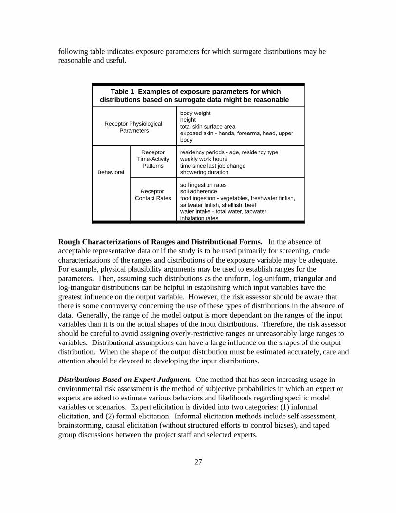
following table indicates exposure parameters for which surrogate distributions may bereasonable and useful.

Table 1 Examples of exposure parameters for whichdistributions based on surrogate data might be reasonable

Receptor Physiological Parameters

body weight height total skin surface areaexposed skin - hands, forearms, head, upperbody

Behavioral showering duration

Receptor residency periods - age, residency typeTime-Activity weekly work hours

Patterns time since last job change

Receptor soil adherenceContact Rates food ingestion - vegetables, freshwater finfish,

soil ingestion rates

saltwater finfish, shellfish, beefwater intake - total water, tapwaterinhalation rates

Rough Characterizations of Ranges and Distributional Forms. In the absence ofacceptable representative data or if the study is to be used primarily for screening, crudecharacterizations of the ranges and distributions of the exposure variable may be adequate. For example, physical plausibility arguments may be used to establish ranges for theparameters. Then, assuming such distributions as the uniform, log-uniform, triangular andlog-triangular distributions can be helpful in establishing which input variables have thegreatest influence on the output variable. However, the risk assessor should be aware thatthere is some controversy concerning the use of these types of distributions in the absence ofdata. Generally, the range of the model output is more dependant on the ranges of the inputvariables than it is on the actual shapes of the input distributions. Therefore, the risk assessorshould be careful to avoid assigning overly-restrictive ranges or unreasonably large ranges tovariables. Distributional assumptions can have a large influence on the shapes of the outputdistribution. When the shape of the output distribution must be estimated accurately, care andattention should be devoted to developing the input distributions.

Distributions Based on Expert Judgment. One method that has seen increasing usage inenvironmental risk assessment is the method of subjective probabilities in which an expert orexperts are asked to estimate various behaviors and likelihoods regarding specific modelvariables or scenarios. Expert elicitation is divided into two categories: (1) informalelicitation, and (2) formal elicitation. Informal elicitation methods include self assessment,brainstorming, causal elicitation (without structured efforts to control biases), and tapedgroup discussions between the project staff and selected experts.

28

Formal elicitation methods generally follow the steps identified by the U.S. NuclearRegulatory Commission (USNRC, 1989; Oritz, 1991; also see Morgan and Henrion, 1990;IAEA, 1989; Helton, 1993; Taylor and Burmaster; 1993) and are considerably more elaborateand expensive than informal methods.

29

References Cited in Text

A. H-S. Ang and W. H. Tang, Probability Concepts in Engineering Planning and Design,Volume I, Basic Principles, John Wiley & Sons, Inc., New York (1975).

D. L. Bloom, et al., Communicating Risk to Senior EPA Policy Makers: A Focus GroupStudy, U.S. EPA Office of Air Quality Planning and Standards (1993).

P. Bratley, B. L. Fox, L. E. Schrage, A Guide to Simulation, Springer-Verlag, New York(1987).

W.S. Cleveland, The Elements of Graphing Data, revised edition, Hobart Press, Summit, New Jersey (1994). W. J. Conover, Practical Nonparametric Statistics, John Wiley & Sons, Inc., New York(1980).

S. H. C. du Toit, A. G. W. Steyn, R.H. Stumpf, Graphical Exploratory Data Analysis,Springer-Verlag, New York (1986).

B. Efron and R. Tibshirani, An introduction to the bootstrap, Chapman & Hall, New York(1993).

M. Evans, N. Hastings, and B. Peacock, Statistical Distributions, John Wiley & Sons, NewYork (1993).

R. O. Gilbert, Statistical Methods for Environmental Pollution Monitoring, Van NostrandReinhold, New York (1987).

J. C. Helton, “Uncertainty and Sensitivity Analysis Techniques for Use In PerformanceAssessment for Radioactive Waste Disposal,” Reliability Engineering and System Safety,Vol. 42, pages 327-367 (1993).

IAEA, Safety Series 100, Evaluating the Reliability of Predictions Made UsingEnvironmental Transfer Models, International Atomic Energy Agency, Vienna, Austria(1989).

N. L. Johnson and S. Kotz, Continuous Univariate Distributions, volumes 1 & 2, John Wiley& Sons, Inc., New York (1970).

M. Kendall and A. Stuart, The Advanced Theory of Statistics, Volume I - DistributionTheory; Volume II - Inference and Relationship, Macmillan Publishing Co., Inc., New York(1979).

30

A. M. Law and W. D. Kelton, Simulation Modeling & Analysis, McGraw-Hill, Inc., (1991).

S. L. Meyer, Data Analysis for Scientists and Engineers, John Wiley & Sons, Inc., New York(1975).

M. G. Morgan and M. Henrion, Uncertainty A guide to Dealing with Uncertainty inQuantitative Risk and Policy Analysis, Cambridge University Press, New York (1990).

NCRP Commentary No. 14, “A Guide for Uncertainty Analysis in Dose and Risk AssessmentsRelated to Environmental Contamination,” National Committee on Radiation Programs,Scientific Committee 64-17, Washington, D.C. (May, 1996).

N. R. Oritz, M. A. Wheeler, R. L. Keeney, S. Hora, M. A. Meyer, and R. L. Keeney, “Use ofExpert Judgment in NUREG-1150, Nuclear Engineering and Design, 126:313-331 (1991).

A. C. Taylor and D. E. Burmaster, “Using Objective and Subjective Information to GenerateDistributions for Probabilistic Exposure Assessment,” U.S. Environmental Protection Agency,draft report (1993).

J. W. Tukey, Exploratory Data Analysis, Addison-Wesley, Boston (1977).

USNRC, Severe Accident Risks: An Assessment for Five U.S. Nuclear power Plants (secondpeer review draft), U.S. Nuclear Regulatory Commission, Washington, D.C. (1989).

31

References for Further Reading

B. F. Baird, Managerial Decisions Under Uncertainty, John Wiley and Sons, Inc., NewYork (1989).

D. E. Burmaster and P. D. Anderson, “Principles of Good Practice for the Use of MonteCarlo Techniques in Human Health and Ecological Risk Assessments,” Risk Analysis, Vol.14(4), pages 477-482 (August, 1994).

R. Clemen, Making Hard Decisions, Duxbury Press (1990).

D. C. Cox and P. Baybutt, “Methods for Uncertainty Analysis: A Comparative Survey,” RiskAnalysis, Vol. 1 (4), 251-258 (1981).

R. D'Agostino and M.A. Stephens (eds), Goodness-of-Fit Techniques, Marcel Dekker, Inc.,New York (1986).

L. Devroye, Non-Uniform Random Deviate Generation, Springer-Verlag, (1986).

D. M. Hamby, “A Review of Techniques for Parameter Sensitivity Analysis of EnvironmentalModels,” Environmental Monitoring and Assessment, Vol. 32, 135-154 (1994).

D. B. Hertz, and H. Thomas, Risk Analysis and Its Applications, John Wiley and Sons, NewYork (1983).

D. B. Hertz, and H. Thomas, Practical Risk Analysis - An Approach Through Case Studies,John Wiley and Sons, New York (1984).

F. O. Hoffman and J. S. Hammonds, An Introductory Guide to Uncertainty Analysis inEnvironmental and Health Risk Assessment, ES/ER/TM-35, Martin Marietta (1992).

F. O. Hoffman and J. S. Hammonds, “Propagation of Uncertainty in Risk Assessments: TheNeed to Distinguish Between Uncertainty Due to Lack of Knowledge and Uncertainty Due toVariability,” Risk Analysis, Vol. 14 (5), 707-712 (1994).

R. L. Iman and J. C. Helton, “An Investigation of Uncertainty and Sensitivity AnalysisTechniques for Computer Models,” Risk Analysis, Vol. 8(1), pages 71-90 (1988).

R. L. Iman and W. J. Conover, “A Distribution-Free Approach to Inducing Rank CorrelationAmong Input Variables,” Commun. Statistics, Communications and Computation, 11, 311-331 (1982).

32

R. L. Iman, J. M. Davenport, and D. K. Zeigler, “Latin Hypercube Sampling (A ProgramUsers Guide),” Technical Report SAND 79:1473, Sandia Laboratories, Albuquerque (1980).

M. E. Johnson, Multivariate Statistical Simulation, John Wiley & Sons, Inc., New York(1987).

N. L. Johnson, S. Kotz and A. W. Kemp, Univariate Discrete Distributions, John Wiley &Sons, Inc., New York (1992).

R. LePage and L. Billard, Exploring the Limits of Bootstrap, Wiley, New York (1992).

J. Lipton, et al. “Short Communication: Selecting Input Distributions for Use in Monte CarloAnalysis,” Regulatory Toxicology and Pharmacology, 21, 192-198 (1995).

W. J. Kennedy, Jr. and J. E. Gentle, Statistical Computing, Marcel Dekker, Inc., New York(1980).

T. E. McKone and K. T. Bogen, “Uncertainties in Health Risk Assessment: An IntegratedCase Based on Tetrachloroethylene in California Groundwater,” Regulatory Toxicology andPharmacology, 15, 86-103 (1992).

R. E. Megill (Editor), Evaluating and Managing Risk, Penn Well Books, Tulsa, Oklahoma(1985).

R. E. Megill, An Introduction to Risk Analysis, end Ed. Penn Well Books, Tulsa, Oklahoma(1985).

Palisade Corporation, Risk Analysis and Simulation Add-In for Microsoft Excel or Lotus 1-2-3. Windows Version Release 3.0 User’s Guide, Palisade Corporation, Newfield, New York(1994).

W. H. Press, B. P. Flannery, S. A. Teulolsky, and W. T. Vetterling, Numerical Recipes inPascal: the Art of Scientific Computing, Cambridge University Press (1989).

W. H. Press, S. A. Teulolsky, W. T. Vetterling, and B. P. Flannery, Numerical Recipes inFORTRAN: the Art of Scientific Computing, Cambridge University Press (1992).

W. H. Press, S. A. Teulolsky, W. T. Vetterling, and B. P. Flannery, Numerical Recipes in C:the Art of Scientific Computing, Cambridge University Press (1992).

T. Read and N. Cressie, Goodness-of-fit Statistics for Discrete Multivariate Data, Springer-Verlag, New York (1988).

33

V. K. Rohatgi, Statistical Inference, John Wiley & Sons, New York (1984).

R. Y. Rubinstein, Simulation and the Monte Carlo Method, John Wiley and Sons, New York (1981).

L. Sachs, Applied Statistics - A Handbook of Techniques, Spring-Verlag, New York (1984).

A. Saltelli and J. Marivort, “Non-parametric Statistics in Sensitivity Analysis for ModelOutput: A Comparison of Selected Techniques,” Reliability Engineering and System Safety,Vol. 28, 229-253 (1990).

H. Schneider, Truncated and Censored Distributions form Normal Populations, MarcelDekker, Inc., New York (1986).

F. A. Seiler and J. L. Alvarez, “On the Selection of Distributions for Stochastic Variables,”Risk Analysis, Vol. 16 (1), 5-18 (1996).

F.A. Seiler, “Error Propagation for Large Errors,” Risk Analysis, Vol 7 (4), 509-518 (1987).

W. Slob, “Uncertainty Analysis in Multiplicative Models,” Risk Analysis, Vol. 14 (4), 571-576(1994).

A. E. Smith, P.B. Ryan, J. S. Evans, “The Effect of Neglecting Correlations WhenPropagating Uncertainty and Estimating the Population Distribution of Risk,” Risk Analysis,Vol. 12 (4), 467-474 (1992).

U.S. Environmental Protection Agency, Guidelines for Carcinogenic Risk Assessment,Federal Register 51(185), 33992-34003 (May 29, 1992).

U.S. Environmental Protection Agency, Source Assessment: Analysis of Uncertainty - Principles and Applications, EPA/600/2-79-004 (August, 1978)

U.S. Environmental Protection Agency, Guidelines for Exposure Assessment, FederalRegister 57(104), 22888-22938 (May 29, 1992).

U.S. Environmental Protection Agency, Summary Report for the Workshop on Monte CarloAnalysis, EPA/630/R-96/010 (September, 1996).

34

Figure 1b: Example Monte Carlo Estimate of the CDF for Lifetime Cancer Risk

Figure 1a. Example Monte Carlo Estimate of the PDF for Lifetime Cancer Risk

35

Figure 2: Example Box and Whiskers Plot of the Distribution of Lifetime Cancer Risk