impact of variations on 1-d flow in gas turbine engines via monte carlo ... · turbine engines via...

November 2004

Impact of Variations on 1-D Flow in GasTurbine Engines via Monte Carlo SimulationsKhiem Viet NgoStanford University

Dr. Irem TumerNASA Ames Research Center

NASA/TM-2004-212844

National Aeronautics andSpace Administration

Ames Research CenterMoffett Field, California, 94035-1000

https://ntrs.nasa.gov/search.jsp?R=20040200973 2018-05-29T16:36:04+00:00Z

November 2004

Impact of Variations on 1-D Flow in GasTurbine Engines via Monte Carlo Simulations

NASA/TM-2004-212844

National Aeronautics andSpace Administration

Ames Research CenterMoffett Field, California, 94035-1000

Khiem Viet NgoStanford University

Dr. Irem TumerNASA Ames Research Center

NASATM 2004-212844 Impact of Variations on 1-D Flow in Gas Turbine Engines

Impact of Variations on 1-D Flow in Gas Turbine Engines via Monte Carlo Simulations

Khiem Viet Ngo Graduate Student

Dept. of Aeronautics & Astronautics Stanford University Stanford, CA 94305

(650) 888-4382 [email protected]

Irem Y. Tumer, Ph.D.1 Research Scientist

Computational Sciences Division NASA Ames Research Center Moffett Field, CA 94035-1000

(650) 604 2976 [email protected]

ABSTRACT The unsteady compressible inviscid flow is characterized by the conservations of mass, momentum, and energy; or simply the Euler equations. In this paper, a study of the subsonic one-dimensional Euler equations with local preconditioning is presented using a modal analysis approach. Specifically, this study investigates the behavior of airflow in a gas turbine engine using the specified conditions at the inflow and outflow boundaries of the compressor, combustion chamber, and turbine, to determine the impact of variations in pressure, velocity, temperature, and density at low Mach numbers. Two main questions motivate this research: 1) Is there any aerodynamic problem with the existing gas turbine engines that could impact aircraft performance? 2) If yes, what aspect of a gas turbine engine could be improved via design to alleviate that impact and to optimize aircraft performance? This paper presents an initial attempt to model the flow behavior in terms of their eigenfrequencies subject to the assumption of the uncertainty or variation (perturbation). The flow behavior is explored using simulation outputs from a “customer-deck” model obtained from Pratt & Whitney. Variations of the main variables (i.e., pressure, temperature, velocity, density) about their mean states at the inflow and outflow boundaries of the compressor, combustion chamber, and turbine are modeled. Flow behavior is analyzed for the high-pressure compressor and combustion chamber utilizing the conditions on their left and right boundaries. In the same fashion, similar analyses are carried out for the high-pressure and low-pressure turbines. In each case, the eigenfrequencies that are obtained for different boundary conditions are examined closely

1 Corresponding author A short version of this paper was published in the Proceedings of the IEEE Aerospace Conference, Big Sky, Montana, March 6-13, 2004

1

mailto:[email protected]

mailto:[email protected]


based on their probabilistic distributions, a result of a Monte Carlo 10,000–sample simulation. Furthermore, the characteristic waves and wave response are analyzed and contrasted among different cases, with and without preconditioners. The results reveal the existence of flow instabilities due to the combined effect of variations and excessive pressures in the case of the combustion chamber and high-pressure turbine. Finally, a discussion is presented on potential impacts of the instabilities and what can be improved via design to alleviate them for a better aircraft performance. KEYWORDS Gas turbine engine; Monte Carlo simulation; Aerodynamic measures; Decay rate; Vehicle health monitoring; Flow instability; Characteristic waves and wave response NOMENCLATURE

jα coefficients of the eigenmodes used to determine the wave response ( )ωB combination of and matrices, used to determine the eigenfrequencies

and the characteristic strengths inC outC

c speed of sound inC inflow coefficient matrix

outC outflow coefficient matrix γ specific heat ratio HSP entropy, enthalpy, and pressure boundary conditions HFP mass flux, enthalpy, and pressure boundary conditions

jλ eigenvalues (characteristic speeds) M Mach number p pressure P preconditioner q velocity QTP velocity, temperature, and pressure boundary conditions QRP velocity, density, and pressure boundary conditions ρ density

jr eigenvectors RPP density, pressure, and pressure boundary conditions t time variable

ju eigenmodes (characteristic waves) u wave response (linear superposition of the eigenmodes)

rω the real part of the eigenfrequency

iω the imaginary part of the eigenfrequency ( iω = decay rate) x physical length of a component being considered

2


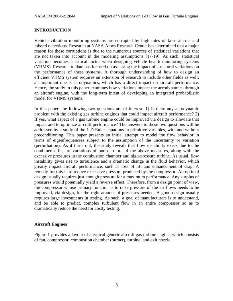
INTRODUCTION Vehicle vibration monitoring systems are corrupted by high rates of false alarms and missed detections. Research at NASA Ames Research Center has determined that a major reason for these corruptions is due to the numerous sources of statistical variations that are not taken into account in the modeling assumptions [17-19]. As such, statistical variation becomes a critical factor when designing vehicle health monitoring systems (VHMS). Research to date has focused on assessing the impact of structural variations on the performance of these systems. A thorough understanding of how to design an efficient VHMS system requires an extension of research to include other fields as well; an important one is aerodynamics, which has a direct impact on aircraft performance. Hence, the study in this paper examines how variations impact the aerodynamics through an aircraft engine, with the long-term intent of developing an integrated probabilistic model for VHMS systems. In this paper, the following two questions are of interest: 1) Is there any aerodynamic problem with the existing gas turbine engines that could impact aircraft performance? 2) If yes, what aspect of a gas turbine engine could be improved via design to alleviate that impact and to optimize aircraft performance? The answers to these two questions will be addressed by a study of the 1-D Euler equations in primitive variables, with and without preconditioning. This paper presents an initial attempt to model the flow behavior in terms of eigenfrequencies subject to the assumption of the uncertainty or variation (perturbation). As it turns out, the study reveals that flow instability exists due to the combined effect of variations of one or more of the above measures, along with the excessive pressures in the combustion chamber and high-pressure turbine. As usual, flow instability gives rise to turbulence and a dramatic change in the fluid behavior, which greatly impact aircraft performance, such as loss of lift and enhancement of drag. A remedy for this is to reduce excessive pressure produced by the compressor. An optimal design usually requires just enough pressure for a maximum performance. Any surplus of pressures would potentially yield a reverse effect. Therefore, from a design point of view, the compressor whose primary function is to raise pressure of the air flows needs to be improved, via design, for the right amount of pressures needed. A good design usually requires large investments in testing. As such, a goal of manufacturers is to understand, and be able to predict, complex turbulent flow in an entire compressor so as to dramatically reduce the need for costly testing. Aircraft Engines Figure 1 provides a layout of a typical generic aircraft gas turbine engine, which consists of fan, compressor, combustion chamber (burner), turbine, and exit nozzle.

3


Figure 1 Pratt & Whitney PW4000 turbofan engine [11]

Air enters at the air intake near the fan and exits out from the nozzle after going through a series of different components. Figure 2 summarizes the investigation performed in this paper: the flow behavior in the high-pressure compressor, burner, high-pressure turbine, and low-pressure turbine with the three boundary conditions Euler Riemann, HSP, and HFP [1]. Input to the simulation are the F117 numerical data, provided by Pratt & Whitney [22], which are applied at the four front boundaries, indicated by the four up arrows, one for each of the above four components.

4


Low PressureCompressor

High PressureCompressor

High PressureTurbine

Low PressureTurbine

1. Euler Riemann Boundary Condition2. Entropy, Enthalpy at Inflow, Pressure at Outflow

3. Mass Flux, Enthalpy at Inflow, Pressure at Outflow

Eigenfrequency Analysis

FlowBehavior

Fan ExitNoz.Burner

x = 0

x = 0

x = 1 x = 1

x = 1

x = 0

Figure 2 Overview of a Typical Aircraft Engine

As the purpose of this paper is to study the impact of variations on the flow, we assume that there are variations in pressure, velocity, density, and temperature about their unperturbed steady states. In addition, we choose the standard deviations to be 10% of the mean values of each of the above measures. With these defined assumptions, the probabilistic distributions of different eigenfrequencies, which are generated from the standard normal distribution of zero mean and standard deviation of 1, are obtained from a 10,000-sample Monte Carlo simulation. Of interest is the case where the altitude is 30,000 feet. In this case, flow behavior is analyzed for the high-pressure compressor and combustion chamber employing the conditions on their left and right boundaries. In the same fashion, similar analyses are carried out for the high-pressure and low-pressure turbines. Figure 3 shows pressure levels of different operating conditions or cases throughout the engine. Figure 4 shows pressure curves at the front boundaries of each component going through different cases. The pressure curves for the combustion chamber and for the high-pressure turbine are just nearly the same. Thus we can expect similar flow behavior in these two components. Likewise, the flow behavior in the low-pressure turbine should look like that in the high-pressure compressor. In addition, Figure 4 shows that there is a pressure-power relationship (the RC codes stand for various power rates). In other words, an increase in pressure is directly proportional to an increase in power and vice versa.

5


This relationship is quite clear when there is a deep drop in pressure in Case 4 due to low power. But then, the pressure quickly makes its way up and achieves a maximum value in Case 5 due to sufficiently high power. On the contrary, there exists a reverse relationship between pressure and altitude; i.e., when an aircraft reaches a higher altitude, the pressure decreases. This can be observed in Case 15 when there is another deep drop in pressure, but this time not because of power. It is obviously due to an increase in altitude. As will be shown in the section to come, under variations in pressure, velocity, density, and temperature, excessively high pressure becomes a leading factor that gives rise to flow instability. Thus, the problem seems to occur even before the takeoff. For this paper, case 14 has been selected for analysis.

F117: Pressure vs Station [Cases 1, 2,...,17]

-50

0

50

100

150

200

250

300

350

400

450

0 2 4 6 8 10 12 14 1

Pres

sure

(psi

)

6

1: RC=50, ALT=0 2: RC=45, ALT=0 3: RC=40, ALT=0 4: RC=20, ALT=05: RC=50, ALT=0 6: RC=50, ALT=0 7: RC=50, ALT=0 8: RC=50, ALT=09: RC=50, ALT=0 10: RC=50, ALT=0 11: RC=50, ALT=5000 12: RC=40, ALT=013: RC=40, ALT=15000 14: RC=40, ALT=30000 15: RC=40, ALT=40000 16: RC=45, ALT=017: RC=45, ALT=15000

Low Pres.

Compr.

High Pres.

TurbineBurner

High Pres.

Compr.

Low Pres.

Turbine

Figure 3 Engine Pressures in Different Cases of Operation

6


F117: Pressure vs Case No.

0

50

100

150

200

250

300

350

400

450

0 2 4 6 8 10 12 14 16 18

Case No.

Pres

sure

(psi

)

High Pressure Compressor Combustion Chamber High Pressure Turbine Low Pressure Turbine

Figure 4 Pressures at the Front Boundaries of Various Components in Different Cases

Aerodynamics of Aircraft Engines In the study of aircraft engines, one aspect that has been the central theme of research is aerodynamics. In particular, the problem of interest has so far been the Euler equations, which consist of the three fundamental conservation equations of aerodynamics, namely mass, momentum, and energy. These coupled equations together model the motion of the fluid in a control volume, which, in this paper, includes the high-pressure compressor, combustion chamber, and high- and low- pressure turbines. Due to the geometry of each of these components, it is perfectly valid to describe fluid motion with the 1-D Euler equations, which should also be valid for the quasi 1-D flows. The study here is to employ the 1-D Euler equations to describe the flows through an aircraft gas turbine engine subject to the boundary conditions at the inflow and outflow boundaries. These typically involve thermodynamic conditions such as entropy, stagnation enthalpy at inflow, and pressure at outflow. Likewise, the boundary conditions could be defined by velocity and temperature at inflow and pressure at outflow. The study of the Euler equations can be traced back to the early 1980s when Yee, Beam, and Warming [8, 9] conducted numerical experiments for the one-dimensional inviscid equations of gas dynamics applied to nozzle flows for their research at NASA Ames Research Center by means of similarity transformation and finite difference analysis. A year later, Michael Giles [1] of MIT, during his visit at NASA Langley Research Center,

7


further studied the Euler equations with different types of boundary conditions. And most recently, David Darmofal [2] of MIT brought the work to one more level by exploring the flow behavior under the impact of preconditioning. In this paper, we take a look at the Euler equations from a probabilistic perspective. Unlike the above authors’ research whose efforts are oriented toward the numerical solution of a computational fluid dynamic problem, the interest here is geared toward the analysis of flow behavior in a gas turbine engine (namely, the compressor, combustion chamber, and turbine) under the impact of variations given the specified conditions at each boundary, via the Euler equations. From a mathematical point of view, the Euler equations are a set of nonlinear, coupled, hyperbolic differential equations (HDEs). The HDEs have two important properties: 1) they allow discontinuous solutions (in physical terms, this means that the flow can contain shocks or contact discontinuities); 2) the solution can be expressed as a linear combination of the eigenmodes (three in the case of a one-dimensional problem). The three eigenmodes are called characteristic waves and are physically associated with the characteristic speeds (the eigenvalues), the velocity of the flow, and the velocity of sound. The physical relevance of this is that in a gas, no signal can travel faster than the speed of sound, and consequently the eigenvalues are the highest possible signal speed within a flow. Also, if a shock occurs, its effect will spread with the characteristic speeds. In other words, the eigenvalues are the shock speeds. The intention of this paper is not about shocks, as this topic has been studied extensively by many researchers ([2], [8], and [9] as an example). As of today, several studies have been aimed at the one-dimensional Euler equations with different types of preconditioners [1, 2, 3, 4, 5, 6, 7]. As pointed out by Godfrey [6], when the Euler equations become poorly coupled due to the vast difference in rates between the acoustic and convective waves, the system’s condition number becomes high. As such, stiffness results in causing numerical solutions to converge slowly and contain large uncertainties. A preconditioner is a matrix that is used to reduce the spread of the speed of these waves, to optimize the condition number, to accelerate convergence of the response (waves) to steady state, and to decrease the solution’s uncertainty. These preconditioning matrices have been studied and designed by several authors and hence are not the subject of discussion in this paper. Rather, they are used in the analysis of waves that enter and leave a gas turbine engine under the influence of the boundary conditions mentioned above. As mentioned in [7], high-speed flow solutions are unaffected by preconditioning whereas low-speed flow solutions demonstrate that preconditioning is essential if density-based methods are used. Also, since the Euler equations are for compressible flows, we are to look at the flow behaviors in the subsonic compressible flows, 0.3 , of which density is a variable. We will soon show that preconditioning, though having good effects in deterministic approach, has a reverse effect in probabilistic approach where variations in pressures, temperatures, velocities, and densities are assumed.

1M< <

8


To gain a fundamental understanding of the impact of variations on the wave performance, an investigation of the preconditioned 1-D Euler equations is carried out by means of modal analysis with various boundary conditions. The study will employ some typical symmetric preconditioners, namely the van Leer-Lee-Roe and the optimal preconditioners. In each case, the eigenfrequency will be determined deterministically. In addition, Monte Carlo simulations will be used to explore the impact of variations of aerodynamic measures on the flows at those boundaries. MATHEMATICAL FOUNDATION As our analysis is based on Giles’ and Darmofal’s work, the following mathematical formulations come directly from their papers [1-2], repeated here for convenience, to include the results on the characteristic waves and wave response under various boundary conditions. The extension of their study begins with Table 1 where eigenfrequencies are to be stochastically analyzed to gain further understanding of the flow behavior in gas turbine engines, under the assumption of variations (disturbances) of pressure, velocity, density, and temperature. The one-dimensional preconditioned Euler equations are given by

1

2

0 000 0

T X

qq q qp c q p

ρ ρ ρρ

ρ

−

⎡ ⎤ ⎡ ⎤ ⎡ ⎤ ⎡ ⎤⎢ ⎥ ⎢ ⎥ ⎢ ⎥ ⎢ ⎥=⎢ ⎥ ⎢ ⎥ ⎢ ⎥ ⎢ ⎥⎢ ⎥ ⎢ ⎥ ⎢ ⎥ ⎢ ⎥⎣ ⎦ ⎣ ⎦ ⎣ ⎦ ⎣ ⎦

+ P% %

% %

% %

0 (1)

where ρ% , and are the perturbation density, velocity, and pressure and ,~q p~ ρ , ,q and p are the mean density, velocity, and pressure, respectively; c is the speed of sound;

2c pγ ρ= ; and P is a preconditioning matrix. To simplify the analysis, a transformation of (1) is made based on the following non-dimensionalizations:

2, , , ,q q c p p c x X L t Tc Lρ ρ ρ ρ≡ ≡ ≡ ≡ ≡% % % . It follows that (1) becomes

t x+ =u PAu 0 (2) where

qp

ρ⎡ ⎤⎢ ⎥= ⎢ ⎥⎢ ⎥⎣ ⎦

u , and 1 0

0 10 1

MM

M

⎡ ⎤⎢ ⎥= ⎢ ⎥⎢ ⎥⎣ ⎦

A ,

9


Here, M is the mean Mach number ( cqM = ). With the inflow and outflow boundary conditions defined in [2], equation (2) forms a set of initial boundary value problems. Assuming each eigenmode of (2) is of the form ( , ) exp[ ( )]j j jx t i k x tω= −u r (3) Upon substitution, (2) results in an eigenvalue problem ( )j jλ− =PA I r 0 (4) where j jkλ ω= and are the eigenvalues and eigenvectors of PA respectively. jrBy allowing the wave response to represent interactions among the eigenmodes, we let

be a linear superposition of these three modes: u

u

3 3

1 1

exp( )i tj j j j j

j j

e iω xα α ω−

= =

= =∑ ∑u u r λ (5)

To extend Giles’ and Darmofal’s work [1, 2] on the one-dimensional preconditioned Euler equations, it is necessary to revisit their use of different boundary conditions, namely a) the Euler Riemann invariant condition; b) the entropy, stagnation enthalpy at inflow, and pressure at outflow (HSP conditions), a common set of boundary conditions for subsonic internal flows; c) the mass flux, stagnation enthalpy at inflow, and pressure at outflow (HFP conditions); d) the velocity, temperature at inflow, and pressure at outflow (QTP conditions), another frequently used set of boundary conditions in low-speed viscous flow applications; e) the density, pressure at inflow, and pressure at outflow (RPP conditions); and f) the density, velocity at inflow, and pressure at outflow (QRP conditions). In general, the specified boundary condition at outflow is pressure. Inflow boundary specification requires two conditions, which could be a permutation of the set of entropy, enthalpy, mass flux, velocity, temperature, and pressure. For simplicity, let us assume that the inflow boundary is at x = 0 and the outflow boundary at

where L is the physical length of the domain considered. Below is a summary of the aforementioned boundary conditions.

1,x L= =

a. Euler Riemann Invariant

' '0, 2 2' '

1 12 2, ' '

1 1

p px

q c q c

x L q c q

γ γρ ρ

γ γ

γ γ

⎧ =⎪= ⎨ + = +⎪

c

− −⎩

= − = −− −

(6)

where the primed quantities denote the sum of the mean and perturbation states

10


b. HSP conditions

2 2

' '0, 1 ' 1'

2 1 ' 2, '

p px

1p pq q

x L p p

γ γρ ργ γ

γ ρ γ

⎧ =⎪= ⎨ + = +⎪ − −⎩

= =

ρ (7)

c. HFP conditions

2 2

' '0, 1 ' 1'

2 1 ' 2, '

q qx

1p pq q

x L p p

ρ ργ γ

γ ρ γ

=⎧⎪= ⎨ + = +⎪ − −⎩

= =

ρ (8)

d. QTP conditions

' '

0,'

, '

p px

q qx L p p

ρ ρ=⎧= ⎨ =⎩= =

(9)

e. RPP conditions

'

0,'

, '

xp p

x L p p

ρ ρ=⎧= ⎨ =⎩= =

(10)

f. QRP conditions

'

0,'

, '

xq q

x L p p

ρ ρ=⎧= ⎨ =⎩= =

(11)

In this paper, the first four boundary conditions will be considered. The RPP conditions, as shown by Giles, led to an ill-posed problem due to the existence of one zero eigenfrequency. Likewise, the QRP conditions, although well posed, result in zero decay rates of the eigenmodes, resulting in their sinusoidal response continuing indefinitely with the same amplitude. Such a behavior clearly fails to capture any

11


variations or disturbances in aerodynamic measures of quantities such as pressure, velocity, density, or temperature, and hence is not considered in this paper. To continue our analysis, each of the above boundary conditions [a-d] is linearized and non-dimensionalized so that each is now of the form

(0, ) 0(1, ) 0

in

out

tt==

C uC u

(12)

where and are the inflow and outflow coefficient matrices (see the Appendix). Available in [1] and [2] is a full analytical derivation of these conditions. In all cases the boundary conditions (equations (12)), expressed again in a more comprehensive manner, are

(2 3)in ×C (1 3)out ×C

[ ]

31 2

1

1 2 2 2

3

1

1 2 2 2

3

00

0

in

ii iout e e e ω λω λ ω λ

ααα

ααα

⎡ ⎤⎡ ⎤⎢ ⎥ = ⎢ ⎥⎢ ⎥ ⎣ ⎦⎢ ⎥⎣ ⎦

⎡ ⎤⎢ ⎥⎡ ⎤ =⎣ ⎦ ⎢ ⎥⎢ ⎥⎣ ⎦

C r r r

C r r r

(13)

In a compact expression, the two above equations are written together as

(14) 1

2

3

( ) [0]α

ω αα

⎡ ⎤⎢ ⎥ =⎢ ⎥⎢ ⎥⎣ ⎦

B

Thus each of the boundary conditions Euler Riemann, HSP, HFP, and QTP is represented by a matrix ( ).ωB For nontrivial solution, we required that [ ]det ( ) 0ω =B from which the eigenfrequency of each boundary condition for different preconditioners is determined. In order to investigate the eigenmodes and wave response, the eigenfrequency ω is separated into its real and imaginary parts r i iω ω ω= + . As it turns out, each eigenmode and the wave response u grow exponentially with time as long as the imaginary part of the eigenfrequency iω is positive. Thus, for a decaying solution, we require that iω be negative and hence iω is the decay rate. Omitting the lengthy algebraic details, the results of rω and iω obtained for the above boundary conditions, with and without preconditioner, are summarized in Table 1 below.

12


Without Preconditioner Eigenfrequencies (Real & Imag. Parts)

a. Euler Riemann Invariant 2 ( 1)n M ,rω π= − n ∈Z

i

ω = −∞

b. Entropy and Enthalpy at Inflow, Pressure at Outflow

2( 1) ,2r

n Mπω −= ∈Z n

2 1 1log2 1i

M MM

ω − +=

−

c. Mass Flux and Enthalpy in Inflow, Pressure at Outflow

2(1 )( 1 2) ,r M nω π= − + n∈Z2 1 (1 )(1 )log2 (1 )(1i

M M MM M M

γωγ )

M⎡ ⎤− + − += ⎢ ⎥− + −⎣ ⎦

d. Velocity and Temperature at Inflow, Pressure at Outflow

2(2 1)( 1) ,2r

n Mπω + −= n∈Z

0iω = Van Leer-Lee-Roe Preconditioner VLRP Eigenfrequencies (Real & Imag. Parts)

a. Euler Riemann Invariant ,r Mnω π= n∈Z

1log2 1iM M

Mω +

= −−


2 ,r Mnω π= n∈Z

iω = −∞

c. Mass Flux and Enthalpy at Inflow, Pressure at Outflow

,r Mnω π= n∈Z

iω = −∞


2 ,r Mnω π= n∈Z

iω = −∞ Optimal Preconditioner JP Eigenfrequencies (Real & Imag. Parts)

a. Euler Riemann Invariant 0r ω =

iω = −∞


,r Mnω π= n∈Z 1log

2 1iM M

Mω +

= −−

c. Mass Flux and Enthalpy at Inflow, Pressure at Outflow

(2 1 2) ,r M nω π= + n∈Z (1 )(1 )log

2 (1 )(1iM M M

M M Mγωγ )

M⎡ ⎤+ − += − ⎢ ⎥− + −⎣ ⎦


(2 1) ,2r

n Mπω += n∈Z

0iω =

Table 1 Eigenfrequencies for Various Boundary Conditions

13


From Table 1, it is clear that the imaginary part of the eigenfrequency is zero under the QTP conditions when no preconditioning is applied. Thus, the decay rate is zero. However, what is interesting about this case is that the decay rates become infinite when the Euler equations are preconditioned by the Van Leer-Lee-Roe preconditioner, which immediately shows an effect of preconditioning. Notice that the decay rates remain zero under the optimal preconditioner condition; this shows that the decay rates can greatly vary from one preconditioner to another. Like the QTP conditions, the QRP also results in zero decay rates and they could certainly be made infinite if an appropriate preconditioner is applied. Now that the QTP conditions yield decay rates of either zero or infinity, these conditions are clearly independent from any variations that may exist in pressure, velocity, density, and temperature. Therefore, we eliminate them from further consideration. Back to Table 1, by splitting the eigenfrequency into its real and imaginary parts, equation (5) can be recast as follows:

3

1

( , ) (cos sin ) exp( )

cos sin exp

r r i

ir rj j

j j j

x t t i t t

j

x i x x

ω ω ω

ωω ωαλ λ λ=

= − ×

⎡ ⎤ ⎡⎛ ⎞ ⎛ ⎞ ⎛ ⎞+ −

⎤⎢ ⎥ ⎢⎜ ⎟ ⎜ ⎟ ⎜ ⎟⎜ ⎟ ⎜ ⎟ ⎜ ⎟ ⎥⎢ ⎥ ⎢⎝ ⎠ ⎝ ⎠ ⎝ ⎠ ⎥⎣ ⎦ ⎣

∑

u

r⎦

1

(15)

where 0 . It follows that the flow amplitude between the two boundaries x = 0 and x = L = 1 is determined by the inequality

x L≤ ≤ =

( )3 3

22 21 1

exp( ) exp ( , )i j j i j jj j

t x tω α ω λ α= =

− ≤ ≤∑ ∑r u jr (16)

In view of (16), the real part of the mean eigenfrequency plays no role in determining the amplitude of the wave response. It is determined by four factors beside the time and space variables: the eigenvectors the coefficients ,jr ,jα the imaginary part of the mean eigenfrequency ,iω and the eigenvalues jλ . While the latter three are mostly dependent upon variations in pressure, velocity, density, and temperature, the first not always is, as shown in Table 2 below. In addition, equation (16) assumes t = 0 at x = 0. Note that in the event that the imaginary part of the eigenfrequency is negative infinity, the term exp( )itω vanishes while the other term exp( )i jxω λ− seems to become positive infinity as long as one of the eigenvalues is positive. Consequently, the eigenmodes would not exist unless the eigenvalues of the resultant matrix PA are all negative. The following mathematical analysis reveals that when ,iω = −∞ the term exp( )i jxω λ− can be made to decay as long as the real part of the eigenfrequency is chosen to be negative. Recall that

,j k jλ ω= so the term exp( ) exp( )i j i jx k xω λ ω ω− = − . Considering the exponent of the exponential, we have

14


2

2i j r i j i j

r i

k x k x k xi

iω ω ω ωω ω ω ω

− = − ++ 2 (17)

The imaginary part is certainly not a matter of concern. As for the real part, if rω is chosen to be negative, then 0.r r rω ω ω− = = > It follows that

2 2exp exp exp 0r i j r i j i j

rr

k x k x k xω ω ω ω ωωω ω

⎛ ⎞ ⎛ ⎞ ⎛ ⎞⎜− ⎟ ≤ ⎜ ⎟ = →⎜ ⎟⎜ ⎟⎜ ⎟ ⎜ ⎟ ⎝ ⎠⎝ ⎠ ⎝ ⎠

(18)

as .iω → −∞ In addition, for the imaginary part, we have

(22

2 2exp exp expi j jj

k x k xk x

ω ω

ω ω

⎛ ⎞⎛ ⎞⎜ ⎟⎜ ⎟ ≤ =

⎜ ⎟ ⎜ ⎟⎝ ⎠ ⎝ ⎠) (19)

In short, for those boundary conditions that result in iω being negative infinity, the decay rates become infinite. Disturbances in all three characteristic waves and the wave response quickly vanish in finite time. Thus, remaining in our analysis are the cases when the iω is in the range 0.iω−∞ < < Table 2 below summarizes the elements that determine the eigenmodes and wave response. Case No / BC Conditions Coefficients Eigenvalues / Eigenvectors

HSP boundary condition

1

2

3

011

MM

ααα

== += −

1

2

3

11

MMM

λλλ

== −= +

[ ][ ][ ]

1

2

3

1 0 0

1 1 1

1 1 1

T

T

T

=

= −

=

r

r

r

Without Preconditioner

HFP boundary condition

1 2 3

3

2

1 1

(1 )(1 )(1 )(1 )

M MM M

M M MM M M

α α α

α γα γ

+ −= − +

+ − +=

− + −

1

2

3

11

MMM

λλλ

== −= +

[ ][ ][ ]

1

2

3

1 0 0

1 1 1

1 1 1

T

T

T

=

= −

=

r

r

r

Leer-Lee-Roe Preconditioner

Euler Riemann boundary condition

1

2

3

01

1M

ααα

== − +=

1

2

3

MM

M

λλλ

=== −

[ ][ ][ ]

1

2

3

1 0 0

0 1 0

1

T

T

TM M

=

=

= −

r

r

r

Table 2 Coefficients, Eigenvalues, and Eigenvectors for Various Boundary Conditions

Since these analyses are eigenfrequency based, let us turn our attention to the eigenfrequencies in Table 2 above. From modal analysis, it has been determined that there exists an infinite set of discrete eigenfrequencies for each boundary condition, with

15


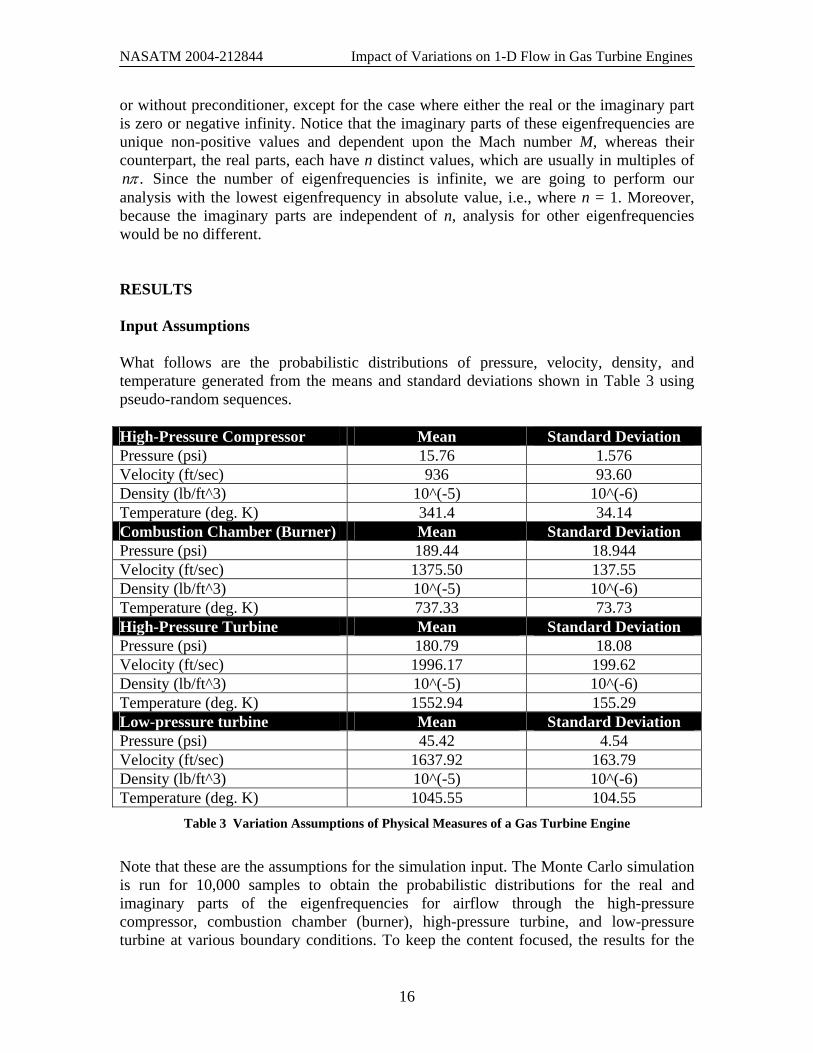
or without preconditioner, except for the case where either the real or the imaginary part is zero or negative infinity. Notice that the imaginary parts of these eigenfrequencies are unique non-positive values and dependent upon the Mach number M, whereas their counterpart, the real parts, each have n distinct values, which are usually in multiples of

.nπ Since the number of eigenfrequencies is infinite, we are going to perform our analysis with the lowest eigenfrequency in absolute value, i.e., where n = 1. Moreover, because the imaginary parts are independent of n, analysis for other eigenfrequencies would be no different. RESULTS Input Assumptions What follows are the probabilistic distributions of pressure, velocity, density, and temperature generated from the means and standard deviations shown in Table 3 using pseudo-random sequences. High-Pressure Compressor Mean Standard Deviation Pressure (psi) 15.76 1.576 Velocity (ft/sec) 936 93.60 Density (lb/ft^3) 10^(-5) 10^(-6) Temperature (deg. K) 341.4 34.14 Combustion Chamber (Burner) Mean Standard Deviation Pressure (psi) 189.44 18.944 Velocity (ft/sec) 1375.50 137.55 Density (lb/ft^3) 10^(-5) 10^(-6) Temperature (deg. K) 737.33 73.73 High-Pressure Turbine Mean Standard Deviation Pressure (psi) 180.79 18.08 Velocity (ft/sec) 1996.17 199.62 Density (lb/ft^3) 10^(-5) 10^(-6) Temperature (deg. K) 1552.94 155.29 Low-pressure turbine Mean Standard Deviation Pressure (psi) 45.42 4.54 Velocity (ft/sec) 1637.92 163.79 Density (lb/ft^3) 10^(-5) 10^(-6) Temperature (deg. K) 1045.55 104.55

Table 3 Variation Assumptions of Physical Measures of a Gas Turbine Engine

Note that these are the assumptions for the simulation input. The Monte Carlo simulation is run for 10,000 samples to obtain the probabilistic distributions for the real and imaginary parts of the eigenfrequencies for airflow through the high-pressure compressor, combustion chamber (burner), high-pressure turbine, and low-pressure turbine at various boundary conditions. To keep the content focused, the results for the

16


optimal preconditioner are not included since they are as similar as those obtained by the van Leer-Lee-Roe. Figure 5 below shows the distributional characteristics of these input variables for the high-pressure turbine. Similar distributional characteristics are assumed for the high-pressure compressor, combustion chamber, and low-pressure turbine.

Figure 5 (a,b,c,d) Simulation Input Assumptions – High-Pressure Turbine

Probabilistic Analysis and Comparisons of the Results Before going into the probabilistic analysis, it is worthwhile to take a look again at the behavior of airflow described by equation (15). Note that the term exp( )itω controls the decaying behavior of the characteristic waves whereas the other term exp( )i jxω λ− controls the amplitudes of the characteristic waves. Therefore, when decay rates are small, the wave transients become longer with reduced amplitudes, thereby enforcing steady state convergence. However, as we will show later, this is only true without variations. With variations, a state of steadiness can never be reached, due to the combined effect of variations and excessive pressures in the combustion chamber and in the high-pressure turbine. Under these conditions, the three characteristic waves and the wave response are persistently composed of series of resonances with sharp amplitudes. More of this will be mentioned again in the eigenmode discussion section when the picture becomes clearer. Figure 6 through Figure 11 present the comparisons and contrasts of flow behaviors among different boundary conditions, with and without preconditioning.

17


High-Pressure Compressor Combustion Chamber

I. Without Preconditioner

Figure 6 (a,b) HSP conditions

Figure 7 (a,b) HFP conditions

II. Van Leer-Lee-Roe Preconditioner

Figure 8 (a,b) Euler Riemann conditions

18


High-Pressure Turbine Low-Pressure Turbine I. Without Preconditioner

Figure 9 (a,b) HSP conditions

Figure 10 (a,b) HFP conditions


Figure 11(a,b) Euler Riemann conditions

19


1. HSP vs. HFP – High-Pressure Compressor From the histogram results, it is seen that the HSP and HFP conditions, Figure 6a and Figure 7a, have relatively the same effect in terms of the amplitudes of the characteristic waves, though the real parts of the eigenfrequencies are very different between the two conditions. In either condition, the decay rate attains a probability of occurrence of 80% within the vicinity of its mean values under no preconditioning, meaning that the airflow decaying behaviors and transient responses, as well as wave amplitudes of each characteristic wave, are deterministic under any circumstances, with or without the impact of variations.

2. HSP vs. HFP – Combustion Chamber As for the airflow in the combustion chamber, Figure 6b and Figure 7b, their behaviors are quite hard to predict because of low probabilities of occurrence due to a spread-out histogram. As such, there are many possible decay rates, and the transient responses and amplitudes can vary fairly large. In general, airflow behaviors in the combustion chamber are relatively complex to determine regardless of what boundary condition, HSP or HFP, is used, as they both have relatively the same effect on the flows.

3. HSP vs. HFP – High-Pressure Compressor vs. Combustion Chamber, Without

Preconditioner Little has been said about fluid behaviors as the flow enters the combustion chamber, but a general picture is that the flows become increasingly complex due to the combined effect of variations and raising pressures there; see Figure 6(a,b) and Figure 7(a,b). From the simulation input assumption in Table 3, and the fact that Mach number is a ratio between flow velocity and speed of sound while the speed of sound depends on pressure and density, it is clear that the complexity of the flows in the combustion chamber is dominantly due to pressure and not to other minor factors, such as temperature or velocity. Table 3 shows that the pressure in the combustion chamber is more than ten times that in the high-pressure compressor, while the elevations in temperature and velocity are quite small. Note that in the high-pressure compressor the pressure there is totally insignificant compared to that in the combustion chamber. Therefore, the flows in the high-pressure compressor are generally more stable.

4. Euler Riemann Invariant – High-Pressure Compressor vs. Combustion

Chamber With Leer-Lee-Roe Preconditioner In general, a recorded effect of preconditioning in the high-pressure compressor and combustion chamber is that 1) the real parts of the eigenfrequencies become positive, 2) the imaginary parts are shifted closer to the origin with a relatively high probability of occurrence: nearly 30% around the mean values in the high-pressure compressor and 22.5% in the combustion chamber; see Figure 8(a,b). As a result, the amplitudes of the characteristic waves and the wave response increase as a consequence of the reduced decay rates. It follows that the transients of these waves become much longer. The problem is not so serious in compressors but it gets worse in the combustion chamber where pressures are substantially high. In fact, these effects are

20


not caused solely by pressure but by the combined effect of variations and excessive pressures. It is best observed from the effect of the van Leer-Lee-Roe preconditioner where the range of decay rates in the combustion chamber decreases by exactly a factor of 10 in magnitude compared to those in the high-pressure compressor, while the mean decay rate decreases by a factor of 6.5. This means that for the combustion chamber, each characteristic wave has a transient response that is at least six times as long as that of the high-pressure compressor. This increase in transient response couples with a decrease in the amplitude of each eigenmode, and thereby enforces steady state convergence. This seems possible since the real parts in the high-pressure compressor also decrease in magnitude when a preconditioner is applied. It will be shown in the eigenmode analysis section that preconditioning has a reverse effect when it comes to variations. In fact, it turns the relatively smooth characteristic waves into those composed of sharp resonances. Of course, the overall behavior of the characteristic waves and the wave response does decay but they are worsened by resonances, which make the flows unstable.

5. HSP vs. HFP – High-Pressure Turbine

From Figure 4, the pressure curve for the high-pressure turbine nearly resembles that for the combustion chamber, and one can predict the flows should not be much different between these two control volumes. Indeed, the fluid behaviors here are just as complex as those in the combustion chamber because of many possible decay rates, each with a low probability of occurrence, as seen in Figure 9a and Figure 10a. This causes the flows to become unstable in a sense of erratically and persistently fluctuated amplitudes. In terms of decay rates, transient responses, and amplitudes, the two conditions HSP and HFP have relatively the same impact on the flows since the fluid behaviors are globally alike between the two boundary conditions.

6. HSP vs. HFP – Low-Pressure Turbine

Again from Figure 4, one can predict that the flows in the low-pressure turbine are somewhat like those in the high-pressure compressor. The same situation is repeated here. Hence, one can understand the fluid behaviors in the turbines by first starting to learn and understand them in the high-pressure compressor and the combustion chamber. Just like what happens in the high-pressure compressor, the air flows here are quite deterministic under any circumstances, with or without variations. Figure 9b and Figure 10b show that the decay rates under HSP and HFP conditions are 85% in the neighborhood of their mean values. Such a high probability dictates that the flows are well predicted in the low-pressure turbine despite variations of any sort. Globally speaking, there is not much difference in the fluid behaviors between the two boundary conditions.

7. HSP vs. HFP – High-Pressure Turbine vs. Low-Pressure Turbine – No

Preconditioner Much of the information regarding the changes in fluid behaviors as the flows enter the low-pressure turbine from the high-pressure turbine has been previously mentioned. The situation here is just like a reverse process of the flows when they enter the combustion chamber from the compressor. Basically, in terms of the global

21


behavior of the flows, there is no significant difference between the HSP and HFP conditions. The real part of the eigenfrequency is the only major difference between them. In brief, the flows become gradually stable when they enter further into the low-pressure turbine.

8. Euler Riemann Invariant – High-Pressure Turbine vs. Low-Pressure Turbine

With Leer-Lee-Roe Preconditioner Recall that we are only interested in the boundary conditions that yield non-zero finite decay rates. As such, the Euler Riemann Invariant boundary condition remains the only condition analyzed under the effect of a preconditioning. Since flows under the HSP and HFP conditions are not preconditioned, comparisons of the Euler Riemann with either one of these are not appropriate. In general, the effect of preconditioning, Figure 11(a,b), is to increase the magnitudes of the eigenfrequencies (the imaginary part remains negative!) in the low-pressure turbine (and high-pressure compressor) so that the eigenmode and wave response quickly decay in time.

Eigenmode Analysis Finally, we would like to briefly discuss the amplitude plots of the eigenmodes and their linear combinations versus time, shown in Figure 12 through Figure 17. Note that these figures would be the same if plotted versus x. It is because x and t are both arrays made of the same number of step sizes. Therefore, there is a one-to-one correspondence between the two arrays. In this calculation, the time step size is chosen to be 0.05 and space step size 0.01. Much of what is going on here has been captured in the probabilistic analysis section. The plots of the characteristic waves and wave response are just an explicit illustration of the Monte Carlo results. Here, a big picture of the fluid behaviors can easily be seen and that flow instability exists as a result of the combined effects of variations and excessive pressures, which are clearly the case in the high-pressure turbine (and in the burner). In addition, the flows under the Euler Riemann invariant condition, with Leer-Lee-Roe preconditioner, show that two of the three characteristic waves have identical amplitudes. As such, they coincide and hence, one can only see two characteristic waves. Likewise, numerical experiments show that the third characteristic wave coincides with the second when the time step approaches zero. This is certainly a matter of interest to numerical analysts, but from our research objective it is not a point of concern. What follows is the eigenmode analysis of the flows, which shows different possible characteristic waves and their linear superimpositions under different boundary conditions.

22


A. High-Pressure Turbine I. Without a Preconditioner

Figure 12 (a,b) HSP condition

Figure 13 (a,b) HFP condition


Figure 14 (a,b) Euler Riemann condition

23


B. Low-Pressure Turbine I. Without a Preconditioner

Figure 15 (a,b) HSP condition

Figure 16 (a,b) HFP condition


Figure 17 (a,b) Euler Riemann condition

24


SUMMARY As mentioned earlier, the goal of this research is to explore the impact of variations on the aerodynamics so that this aspect could be captured in the design of VHMS systems for aerospace devices. In particular, an aerodynamically efficient VHMS system would monitor flow stability in the presence of variations, so that the system could maintain control over the pressures formed in the compressor. Four main findings are highlighted here. The investigation of gas turbine engine air flows at low Mach numbers finds that flow instability exists as a result of the dual effects of variations and high pressures. The problem first initiates in the high-pressure compressor and becomes significant when the flows enter the combustion chamber and the high-pressure turbine in which the pressures there are at least ten times as great. As such, the characteristic waves and the wave response contain plenty of resonance of sharp amplitudes. In other words, with variations in pressure, velocity, density, and temperature assumed, the flows undergo an erratically and persistently fluctuated behavior which does not seem to reach a steady state although they do decay globally. Thus, when variations exist, which is usually the case, pressure becomes the dominant factor that causes the flows to be unstable, as the effects of the other three factors are small. Since flow instability can translate into turbulence in one way or another and thereby impact aircraft performance, this area may require further attention when designing detection systems. The Monte Carlo results show that the fluid flow behaviors are quite deterministic in the high-pressure compressor and the low-pressure turbine since the decay rates there are almost set, with a probability of occurrence of 80% or above, under any circumstances. Thus, the flows in these two components are pretty well predicted whether variations exist or not. On the other hand, the flows become too complex to predict in the combustion chamber and the high-pressure turbine since decay rates here vary greatly, each with a low probability of occurrence. These are the places where the flows become unstable with a possibility of turning into turbulence, and hence may require further attention when designing detection systems. In general, any amount of pressures resulting in flow instability can be considered excessive pressures and would need to be reduced. Recall that high pressures are formed in compressors. Therefore, from a design point of view, some improvements may need to be made toward the high-pressure compressor so that just enough pressures are produced for maximum performance. For example, a reduction in pressure would cause a reduction in thrust, which is required to propel aircraft. This is a challenge for an optimal design since flow stability and thrust force both involve pressure. In addition, Figure 4 shows that power is directly proportional to pressure, giving an alternative toward controlling it. Furthermore, exhibited in Figure 4 is an inverse relationship between pressure and altitude, therefore, flow instability becomes most critical before takeoff. As far as the effect of preconditioning is concerned, eigenmode analysis shows that the problem just gets worse when the Euler equations are preconditioned, at least by the van

25


Leer-Lee-Roe preconditioner under the Euler Riemann Invariant boundary condition, in spite of the usefulness previously shown by several authors in the deterministic case. As we wanted to keep the content focused, results for the optimal preconditioner under the HSP and HFP conditions are not included here. In general, they are just as bad as those in the van Leer-Lee-Roe case. Simply put, preconditioning has a totally reverse effect when it comes to variations even in low pressure; it causes the flows to become unstable with resonance phenomena and prolongs transient response. Hence, preconditioning is not recommended for flows under the impact of variations. ACKNOWLEDGEMENT The authors would like to thank Pratt & Whitney for providing the customer deck model and Bruce Whitney and Kathleen Norkeveck for their insight and patience. REFERENCES [1] Michael Giles, “Eigenmode Analysis of Unsteady One-Dimensional Euler

Equations, ICASE Report No. 83-47, 103915, 1983 [2] David L. Darmofal, “Eigenmode Analysis of Boundary Conditions for the One-

dimensional Preconditioned Euler Equations”, AIAA 99-3352, 14th Computational Fluid Dynamics Conference, Norfolk, VA

[3] David L. Darmofal, Pierre Moinier, and Michael B. Giles, “Eigenmode Analysis of Boundary Conditions for the One-dimensional Preconditioned Euler Equations”, Oxford University Computing Laboratory, Report No. 00/05, March 2000.

[4] David L. Darmofal and Bram V. Leer, “Local Preconditioning of the Euler Equations: A Characteristic Interpretation”, Manuscript.

[5] Michael Giles, “Non-Reflecting Boundary Conditions for the Euler Equations”, CFDL-TR-88-1, Manuscript, February 1998

[6] Andrew G. Godfrey, “Steps Toward a Robust Preconditioning”, AIAA 94-0520, 32nd Aerospace Sciences Meeting & Exhibit, January 10-13, 1994, Reno, NV

[7] Jonathan M. Weiss and Wayne A. Smith, Preconditioning Applied to Variable and Constant Density Flows, AIAA Vol. 33, No. 11, Nov. 1995

[8] H. C. Yee, R. M. Beam, and R. F. Warming, “Boundary Approximations for Implicit Schemes for One-Dimensional Inviscid Equations of Gasdynamics”, AIAA 81-1009R, Vol. 20, No. 9, September 1982

[9] H. C. Yee, R. M. Beam, and R. F. Warming, “Stable Boundary Approximations for a Class of Implicit Schemes for the One-Dimensional Inviscid Equations of Gas Dynamics, AIAA 81-1008

[10] John D. Anderson, Jr., “Fundamentals of Aerodynamics”, McGraw Hill, ISBN: 0-07-237335-0

[11] Philip Hill and Carl Peterson, “Mechanics and Thermodynamics of Propulsion”, Addison Wesley, ISBN: 0-201-14659-2

[12] Klaus Hunecke, “Jet Engines: Fundamentals of Theory, Design and Operation”, ISBN: 0-7603-0459-9

26


[13] Irem Y. Tumer and Anupa Bajwa, “Learning About How Aircraft Engines Work and Fail”, AIAA-99-2850

[14] Mark V. Morkovin, “Recent Insights into Instability and Transition to Turbulence in Open-Flow Systems”, ICASE 110089, NASA Langley Research Center, 1988

[15] D. N. Riahi, “Flow Instability”, WIT Press, ISBN: 1-85312-701-9 [16] Daniel A. McAdams, David Comella, Irem Y. Tumer, “Developing Variational

Vibration Models of Damaged Beams: Toward Intelligent Failure Detection”, Proceedings of IMECE 2003, 2003 ASME International Mechanical Engineering Congress and Expo, November 15-21, 2003, Washington DC, USA. (Journal version in review.)

[17] Daniel A. McAdams and Irem Y. Tumer, “Towards Failure Modeling in Complex Dynamic Systems: Impact of Design and Manufacturing Vibrations”, Proceedings of DETC’02, 2002 ASME Design Engineering Technical Conferences, Sept. 29 – Oct. 2, 2002, Montreal, Quebec, Canada. (Journal version in review.)

[18] Tumer, I. Y., E. M. Huff, “Analysis of Triaxial Vibration Data for Health Monitor-ing of Helicopter Gearboxes”, ASME Journal of Vibration and Acoustics, 2003

[19] Tumer, I. Y., E. M. Huff, “On the Effects of Production and Maintenance Variation on Rotating Machinery Component Performance”, J. of Quality in Maintenance & Engineering, Vol. 8, No. 3, pp. 226-238, 2002

[20] G. Hahn and S. Shapiro, “Statistical Models in Engineering”, Wiley Classic Library ISBN 0-471-04065-

[21] James N. Siddall, “Probabilistic Engineering Design: Principles and Applications”, Marcel Dekker Inc., ISBN 0-8247-7022-6

[22] “User’s Manual for Steady State Performance: F117-PW-100C-17DO-1 Post Flight Status Simulation”, Report No. D 0652151, Pratt & Whitney, United Technologies Corporation

APPENDIX Van Leer-Lee-Roe preconditioner

2

2 2

2 2

01 1

11 01 1

0 0

VLR

M MM MM

M M

1

⎡ ⎤−⎢ ⎥− −⎢ ⎥⎢ ⎥−= ⎢ ⎥− −⎢ ⎥⎢ ⎥⎢ ⎥⎣ ⎦

P

and in terms of the ( , , )q pρ variables,

27


2

2 2

2 2

2

2 2

1 11 1

10 11 1

01 1

M MM M

MM MM M

M M

⎡ ⎤− −⎢ ⎥− −⎢ ⎥

⎢ ⎥= −⎢ ⎥− −⎢ ⎥⎢ ⎥−⎢ ⎥− −⎣ ⎦

Inflow and Outflow Coefficient Matrices

o Euler Riemann conditions

[ ]

1 0 11 1

1 1

in

out

γ γ

γ γ

−⎡ ⎤= ⎢ ⎥− −⎣ ⎦

= − −

C

C

o HSP conditions

[ ]

1 01 ( 1)

0 0 1

in

out

M1

γ γ−⎡ ⎤

= ⎢ ⎥− −⎣ ⎦

=

C

C

o HFP conditions

[ ]

1 01 ( 1)

0 0 1

in

out

MMγ γ

⎡ ⎤= ⎢ ⎥− −⎣ ⎦

=

C

C

o QTP conditions

[ ]

1 00 1 0

0 0 1

in

out

γ−⎡ ⎤= ⎢ ⎥⎣ ⎦

=

C

C

28

REPORT DOCUMENTATION PAGE Form Approved OMB No. 0704-0188

The public reporting burden for this collection of information is estimated to average 1 hour per response, including the time for reviewing instructions, searching existingdata sources, gathering and maintaining the data needed, and completing and reviewing the collection of information. Send comments regarding this burden estimate or any other aspect of this collection of information, including suggestions for reducing this burden, to Department of Defense, Washington Headquarters Services, Directoratefor Information Operations and Reports (0704-0188), 1215 Jefferson Davis Highway, Suite 1204, Arlington, VA 22202-4302. Respondents should be aware thatnotwithstanding any other provision of law, no person shall be subject to any penalty for failing to comply with a collection of information if it does not display a currentlyvalid OMB control number. PLEASE DO NOT RETURN YOUR FORM TO THE ABOVE ADDRESS.1. REPORT DATE (DD-MM-YYYY) 2. REPORT TYPE 3. DATES COVERED (From - To)

4. TITLE AND SUBTITLE 5a. CONTRACT NUMBER

5b. GRANT NUMBER

5c. PROGRAM ELEMENT NUMBER

6. AUTHOR(S) 5d. PROJECT NUMBER

5e. TASK NUMBER

5f. WORK UNIT NUMBER

7. PERFORMING ORGANIZATION NAME(S) AND ADDRESS(ES) 8. PERFORMING ORGANIZATIONREPORT NUMBER

9. SPONSORING/MONITORING AGENCY NAME(S) AND ADDRESS(ES) 10. SPONSORING/MONITOR'S ACRONYM(S)

11. SPONSORING/MONITORINGREPORT NUMBER

12. DISTRIBUTION/AVAILABILITY STATEMENT

13. SUPPLEMENTARY NOTES

14. ABSTRACT

15. SUBJECT TERMS

16. SECURITY CLASSIFICATION OF: 17. LIMITATION OF ABSTRACT

18. NUMBER OFPAGES

19a. NAME OF RESPONSIBLE PERSON

a. REPORT b. ABSTRACT c. THIS PAGE19b. TELEPHONE NUMBER (Include area code)

Standard Form 298 (Rev. 8-98)Prescribed by ANSI Std. Z39-18

7-14-2004 Technical Memorandum Jul 2004 - Nov 2004

Impact of Variations on 1-D Flow in GasTurbine Engines via Monte Carlo Simulations

Khiem Viet Ngo, Stanford University

Dr. Irem Tumer, NASA Ames Research Center

NASA Ames Research CenterMoffett Field, CA 94035-1000

TM-2004-212844

National Aeronautics and Space AdministrationWashington, DC 20546-0001

NASA

TM-2004-212844

Unclassified -- UnlimitedSubject Category 38 Distribution: StandardAvailability: NASA CASI (301) 621-0390

Point of Contact: Dr. Irem Tumer, NASA Ames Research Center, MS 269-1, Moffett Field, CA 94035-1000 (650) 604-2976

In this paper, a study of the subsonic one-dimensional Euler equations with local preconditioning is presented us-ing a modal analysis approach. Specifically, this study investigates the behavior of airflow in a gas turbine engine using the specified conditions at the inflow and outflow boundaries of the compressor, combustion chamber, and turbine, to determine the impact of variations in pressure, velocity, temperature, and density at low Mach numbers. Two main questions motivate this research: 1) Is there any aerodynamic problem with the existing gas turbine engines that could impact aircraft performance? 2) If yes, what aspect of a gas turbine engine could be improved via design to alleviate that impact and to optimize aircraft performance? A discussion is presented on potential impacts of the instabilities and what can be improved via design to alleviate them for a better aircraft performance.

Gas turbine engine; Monte Carlo simulation; Aerodynamic measures; Decay rate; Vehicle health moni-toring; Flow instability; Characteristic waves and wave response

U U U UU 33

302-10-10

impact of variations on 1-d flow in gas turbine engines via monte carlo ... · turbine engines via...

Documents