inflation accounting: what will general price level adjusted income statements show?

CFA Institute

Inflation Accounting: What Will General Price Level Adjusted Income Statements Show?Author(s): Sidney Davidson and Roman L. WeilSource: Financial Analysts Journal, Vol. 31, No. 1 (Jan. - Feb., 1975), pp. 27-31+70-84Published by: CFA InstituteStable URL: http://www.jstor.org/stable/4477780 .

Accessed: 18/06/2014 19:36

Your use of the JSTOR archive indicates your acceptance of the Terms & Conditions of Use, available at .http://www.jstor.org/page/info/about/policies/terms.jsp

.JSTOR is a not-for-profit service that helps scholars, researchers, and students discover, use, and build upon a wide range ofcontent in a trusted digital archive. We use information technology and tools to increase productivity and facilitate new formsof scholarship. For more information about JSTOR, please contact [email protected].

.

CFA Institute is collaborating with JSTOR to digitize, preserve and extend access to Financial AnalystsJournal.

http://www.jstor.org

This content downloaded from 62.122.79.21 on Wed, 18 Jun 2014 19:36:16 PMAll use subject to JSTOR Terms and Conditions

http://www.jstor.org/action/showPublisher?publisherCode=cfa

http://www.jstor.org/stable/4477780?origin=JSTOR-pdf

http://www.jstor.org/page/info/about/policies/terms.jsp


by Sidney Davidson and Roman L. Weil

Inflation Accounting What will general price level

adjusted income statements show?

The most significant and persistent complaint about published financial statements in recent years has been that they do not recognize the economic facts of life. Inflation is a reality throughout the world, yet its effects go unrecog- nized in financial statements prepared in accordance with generally accepted accounting principles in the United States and in most of the other countries of the Western World. Inflation distorts all financial statements, but primary attention in the many public discussions of this topic is usually focused on the way inflation affects reported income. This article analyzes the likely income statement effects of recording inflation adjustments.

Two different approaches to adjusting for inflation have been suggested in the accounting litera- ture. One substitutes for the recorded historical cost data of each of the items in the financial statements the current cost. The other adjusts the recorded historical cost data for changes in the

value of the monetary unit since each item was acquired. The former deals with specific price changes of individual items, the latter with changes in the general price level. Since most adjustments are made by the use of price indexes, the first approach relies on indexes of specific prices, the second on an index of the general price level. The appendix of this article explains and illustrates the essentials of both approaches.

The current cost approach is conceptually su- perior (and presents more meaningful statements) in our view, but the general price-level approach has received authoritative support because of its greater objectivity and auditability. In both the United States and the United Kingdom, the authoritative accounting bodies are currently considering the question of general price-level adjusted financial statements and may issue pro- nouncements requiring their publication in the near future. In both countries, the general price- level statements would be supplemental to the conventional unadjusted historical cost statements. 1

Since general price-level adjusted statements are likely to be the only adjustments for inflation with official sanction, the rest of the body of this article is concerned with the effect of such adjustments on reported earnings. (Some of the results of using current cost adjustments are illustrated in the appendix.)

In the remaining sections we analyze the effects of general price-level adjustments on the 30

Sidney Davidson, Arthur Young Professor of Ac- counting, University of Chicago, is currently on leave as a Fellow of the Center for Advanced Study in the Behavioral Sciences, Stanford, California. Roman L. Weil is Mills B. Lane Professor of Indus- trial Management, Georgia Institute of Technology. The authors thank Christine Ciarfalia and Samy Sidky for their research assistance and the Ford Foundation Faculty Research Fund of the Graduate School of Business of the University of Chicago and the National Science Foundation for research support. They thank Richard M. Cyert, Yuji Ijiri, and Mary Peeler for various kinds of help. 1. Footnotes appear at end of article. (Pp. 83-84)

FINANCIAL ANALYSTS JOURNAL / JANUARY-FEBRUARY 1975 E 27



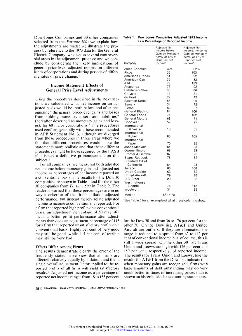
Dow-Jones Companies and 30 other companies selected from the Fortuniie 500; we explain how the adjustments are made; we illustrate the process by reference to the 1973 data for the General Electric Company; we discuss several controver- sial areas in the adjustment process; and we con- clude by considering the likely implications of general price level adjusted reports on different kinds of corporations and during periods of differ- ing rates of price change.2

Income Statement Effects of General Price Level Adjustments

Using the procedures described in the next section, we calculated what net income on an adjusted basis would be, both before and after recognizing -'the general price-level gains and losses from holding monetary assets and liabilities" (hereafter described as monetary gains and losses), for 60 major corporations.3 The procedures used conform generally with those recommended in APB Statement No. 3, although we diverged from those procedures in three areas where we felt that different procedures would make the statements more realistic and that these different procedures might be those required by the FASB if it issues a definitive pronouncement on this subject.'

For all companies, we measured both adjusted net income before monetary gain and adjusted net income as percentages of net income reported on a conventional basis. The results for the Dow 30 companies are shown in Table 1 and for the other 30 companies from Fortllune 500 in Table 2. The reader is warned that these percentages are in no way a criterion of the firm's inflation-adjusted performance, but instead merely relate adjusted income to income as conventionally reported. For a firm that reported high profits on a conventional basis, an adjustment percentage of 80 may still mean a better profit performance after adjustments than does an adjustment percentage of 115 for a firm that reported unsatisfactory profits on a conventional basis. Eighty per cent of very good may still be good, while 115 per cent of terrible may still be very bad.

Effects Differ Among Firms The results demonstrate clearly the error of the frequently stated naive view that all firms are affected relatively equally by inflation, and that a single overall adjustment factor applied to the reported profits of all firms will yield satisfactory results.) Adjusted net income as a percentage of reported net income ranges from 18 to 153 per cent-

Table 1. Dow Jones Companies Adjusted 1973 Income as a Percentage of Reported Income

Adjusted Net Adjusted Net Income before Income, including Gain on Monetary Gain on Monetary Items, as a 0 of Items, as a 0 of Reported Net Reported Net

Company Income* Income*

Allied Chemical 32%/o 62% Alcoa 35 103 American Brands 51 92 American Can 32 83 AT&T 79 153 Anaconda 75 92 Bethlehem Steel 35 86 Chrysler 17 81 du Pont 72 72 Eastman Kodak 86 90 Esmark 34 72 Exxon 82 97 General Electric 84 106 General Foods 71 102 General Motors 68 71 Goodyear 52 95 International

Harvester 10 65 International

Nickel 80 105 International

Paper 70 85 Johns-Manville 84 98 Owens-lilinois 68 98 Procter & Gamble 87 96 Sears, Roebuck 76 82 Standard Oil of

California 84 93 Texaco 83 100 Union Carbide 63 82 United Aircraft 29 18 U.S. Steel 29 68 Westinghouse

Electric 76 112 Woolworth 31 95

Median 68 to 70 92

*See Table 5 for an example of what these columns show.

for the Dow 30 and from 36 to 176 per cent for the other 30. On the Dow list, AT&T and United Aircraft are outliers. If they are eliminated, the range is reduced to a spread from 62 to 112 per cent of conventional income but, of course, this is still a wide spread. On the other 30 list, Trans Union and Loews are high with 176 per cent and 159 per cent, respectively, of reported income. The results for Trans Union and Loews, like the results for AT&T from the Dow list, indicate that when monetary gains are recognized, firms with large amounts of debt outstanding may do very much better in times of increasing prices than is shown on historical dollar accounting statements.

28 [ FINANCIAL ANALYSTS JOURNAL / JANUARY-FEBRUARY 1975



Table 2. Thirty Other Selected Companies from Fortune 500 Adjusted 1973 Income as a Percentage of Reported Income

Adjusted Net Adjusted Net Income before Income, including Gain on Monetary Gain on Monetary Items as a % of Items, as a % of Reported Net Reported Net

Company Incomet Incomet

Avon 93% 100% Baxter Labs 71 100 Brunswick 60 75 Chemetron 10 60 Coca Cola 88 92 Dow Chemical 76 114 Genesco -63" 36 Gould 57 92 Gulf and Western 47 134 Gulf Oil 71 99 Hilton Hotels 61 144 Holiday Inns 70 117 Inland Steel 61 100 IBM 89 93 IT&T 64 108 Koppers 40 61 Loews 70 159 MCA 75 108 Martin Marietta 34 97 Merck 88 85 Pfizer 84 95 Philip Morris 64 108 Pillsbury 45 100 Rockwell

International 84 111 Shell Oil 58 80 Sunbeam 41 56 Trans Union 52 176 Walg reen 7 64 Weyerhauser 88 111 Zenith 78 85

Median 64 99 to 100

aSee Table 5 for an example of what these columns show. bA loss equal to 63 per cent of reported income. See text for explanation of possible cause.

CMerck includes short-term securities with cash. We cannot tell how much they are or what portion of them are nonmonetary. All are included in monetary assets.

Income Before Monetary Gain Reduced for All Firms The figures for adjusted income before monetary gains confirm the often-stated view that conventionally reported earnings have a substantial inflation component. In every case, this partially adjusted income figure was lower than the net income shown in the published financial statements. For the Dow companies the range is from 10 to 87 per cent of conventional income with no conspicuous outliers, although the median of 68 to 70 per cent indicates the distribution is skewed toward the higher percentages. The range of percentages for the other 30 was from -63 to +93 per

cent of reported net income, with a median of 64. Genesco here is clearly an outlier, since Wal-

greens, the next lowest company in these percentages, stands at seven per cent. (The --63 per cent for Genesco means that its adjusted income before monetary gains showed a loss equal to 63 per cent of conventionally reported net income.) The fiscal year for Genesco ended on July 31, 1974. Prices increased during the first half of 1974 at a rate almost twice as large as during the first half of 1973. Thus the results for Genesco may merely indicate that its adjusted income before monetary gain is penalized in our tables because the reporting period for Genesco is significantly different from that for the other companies. To test this, we processed the Genesco data assuming its fiscal year ended on December 31, 1973 (like most of the rest of the 60 companies), but used the same operating data actually reported in the financial statements for the year ending July 31, 1974. In this hypothetical case, Genesco showed a 125 per cent - as opposed to a 163 per cent - decline in income before monetary gain and a 51 per cent - as opposed to a 74 per cent -

decline, in net income. Thus even if Genesco had experienced the lower rate of inflation, it would remain at the bottom of the lists. This analysis raises the point discussed at greater length in the last section of this article: What do we expect to see in the annual reports for the year 1974 when prices increased at a rate much faster than in 1973?

A closer look at the companies in the lower end of the range reveals one possible shortcoming of the method of presentation used here. Inflation adjustments of equal dollar amounts will have a greater percentage effect on the income of a low profit company than on the income of a high profit company. Nineteen seventy-three was not a good year for International Harvester or United Air- craft. The inflation adjustments for International Harvester and United Aircraft, although not especially large relative to other firms, reduced adjusted income before monetary gains to 10 per cent and 18 per cent, respectively, of the modest reported net incomes.

Adjusted Net Income Surprisingly High in Relation to Reported Net Income When monetary gains from net debtor position are included, the resulting net income was a surprisingly high percentage of conventional income (surprising to us and to most other observers, we believe). For the Dow companies, adjusted net income for more than half the companies was 90 per cent or more of reported net income and in seven cases exceeded the reported income. For

FINANCIAL ANALYSTS JOURNAL / JANUARY-FEBRUARY 1975 c 29



the other 30, adjusted income in half the cases was equal to or greater than the reported net income. The significance of the monetary gains factor re- sponsible for these results is discussed in the con- cluding section of this article.

The Estimating Procedure for General Price Level Adjusted Income

The procedure used in making the inflation adjustments reported in the previous section can also be used by analysts in estimating what the general price level adjusted income for any company will be. The procedure requires a copy of the financial statements, including the usual notes, as published in the annual report. An analyst who also has a copy of the Form 10-K filed with the SEC can refine the calculations somewhat, as will be made clear below.

Price Index and Computing Rates of Change in Prices Over Time To compute general price level adjusted income one must have a set of GNP Deflators for each of the five quarters preceding the balance sheet date, plus quarterly or annual data for one or two earlier periods. The handiest source is a table of the GNP Deflator by quarters for the past 10 or 15 years. (An abbreviated list is supplied in a following section.)

Consider, for the purpose of exposition, the problem of analyzing a company whose reporting year ends on December 31, 1974. Assume the GNP Deflator for the fourth quarter of 1974 is reported to be 178 and the GNP Deflator for the fourth quarter of 1973 was reported to be 159.f6

Then the rate of price change for the year 1974 is computed as

178 -_1 = 1.12- 1 = 12 per cent. (1) 159

In the instructions that follow there are statements such as "adjust (a given financial statement item) for one-half year (or some other fraction of a year)." For example, revenues for the year, which are to be adjusted for one-half year of price change, are adjusted six per cent (equal to one- half of 12 per cent).7

In general, if you are required to adjust prices for a fraction of a year, say 62 per cent, then the proportionate price change for that fraction of a year is, in our example, 62 per cent of 12 per cent (=7.44 per cent).8

Adjusting Revenues and Other Income Revenues and other income are, for the most part, spread fairly evenly throughout the year, and adjusting the historically reported amounts for one- half year of price change is usually satisfactory. If the annual report or other information indicates that revenue or other income occurred unevenly throughout the year, then one can adjust that portion of revenues separately.

Adjusting Cost of Goods Sold The adjustment we use for cost of goods sold depends upon whether the company uses a first- in, first-out (FIFO), last-in, first-out (LIFO), or weighted-average cost flow assumption. Some companies use both FIFO and LIFO-one for a part of inventories and the other for the remainder. For those companies we use both the FIFO and LIFO techniques and compute the proper average of the two separate adjustments. (The example discussed later involves this complica- tion.) Companies that merely report using "lower-of-cost-or-market inventory valuation" are assumed to use FIFO, unless the notes give con- trary information.

The adjustment for cost of goods sold requires data from the income statement on cost of goods sold and data on beginning and ending inventories from the balance sheet. If the income statement does not disclose the cost of goods sold, then the notes to the financial statements as reported to the SEC must show it. (The annual report of the (Gen- eral Electric Company, for example, discloses cost of goods sold in the notes to the income statement.)

FIFO Adjustment: Under FIFO, we know that beginning inventory entered cost of goods sold and that the remainder of cost of goods sold consists of the earlier purchases during the year. We assume that the purchases occurred fairly evenly throughout the year. Then the average purchase which entered cost of goods sold was made

Cost of Goods Sold-Beginning Inventory X12 Purchases

x12

months after January 1. Purchases for the year can be computed from the relation

Purchases= Ending Inventory+ Cost of Goods Sold-Beginning Inventory.

General price level adjusted cost of goods sold for FIFO companies is, then,

30 O FINANCIAL ANALYSTS JOURNAL / JANUARY-FEBRUARY 1975



Beginning Inventory Adjusted for a Full Year

plus

Cost of Goods Sold Minus Beginning Inventory Adjusted for the Fraction of a Year Equal to

1 Cost of Goods Sold-Beginning Inventory

L Purchases

X 1/2 -

LIFO Adjustment (Inventory Increase-Normal Case): The adjustment for LIFO cost of goods sold in estimating general price level income depends upon whether inventory increased or de- creased during the year. For most companies, most of the time, inventory amounts increase. The items that enter cost of goods sold under normal conditions are then the later purchases during the year. When inventories are not declining, the average dollar of cost of goods sold was acquired

/2 XCost of Goods Sold x 12 Purchases

months before the end of the year. Thus LIFO cost of goods sold is adjusted for a fraction of the year equal to

Cost of Goods Sold l/2 x

Cost of Goods Sold+Ending Inventory -Beginning Inventory

LIFO Adjustment (Inventory Decrease): When inventory amounts decline during a year, part of cost of goods sold comes from beginning inventory. Under LIFO, the beginning inventory for a year reported on comparative balance sheets is at least two years old as of the current balance sheet date. In our procedures we adjust the "dip into old LI FO layers" for two years, but information in a given annual report may indicate that even more adjustment is necessary. The dip into old LIFO layers is equal to

Beginning Inventory-Ending Inventory

and this amount of cost of goods sold is adjusted for two years of price change, at a minimum. The rest of cost of goods sold (Cost of Goods Sold- Beginning Inventory+Closing Inventory) is adjusted for one-half year of price change.

Weighted-Average Adjustment: Under a weighted-average cost flow assumption, a firm assumes it uses equal portions of all goods available for sale. The total of goods available for sale is beginning inventory plus all purchases, which is also equal to cost of goods sold plus ending inven-

tory. Purchases are assumed to be spread evenly throughout the year. Thus, total goods available for sale in end-of-year dollars is

Beginning Inventory Adjusted for a Full Year

plus

Purchases Adjusted for One-half Year.

The weighted-average cost of goods sold restated in December 31 dollars is

Goods Available Cost of Goods Sold x for Sale Stated Goods Available for Sale in End-of-Year

Dollars

and can be computed as

Cost of Goods Sold Cost of Goods Sold x Ending Inventory

Beginning Cost of Goods Sold Inventory Plus Ending Inventory

x Adjusted for + Minus Beginning Inventory One Year All Adjusted for

One-half year

Adjusting Depreciation To compute price level adjusted depreciation, as- certain the depreciation charges for the year and the accumulated depreciation as of the end of the year. Often, as for example in the annual reports of American Brands (1973) and Sears Roebuck (1974), the amount of depreciation is not shown separately in the income statement, but is included in the cost of goods sold. In that case, the amount of depreciation charges can be read from the statement of changes in financial position. (If depreciation is included in cost of goods sold, then subtract the depreciation from cost of goods sold before adjusting cost of goods sold with the method described in the preceding section.) The amount of accumulated depreciation is shown either directly on the balance sheet or in notes.

If a company uses straight-line depreciation, then the average age of its depreciable assets in years is computed from"'

continued on page 70

REPRINTS of articles published in the Journal are available at a nominal cost. Payment must accompany orders of $10 or less. Address requests to Reprint Department, FAJ.

FINANCIAL ANALYSTS JOURNAL / JANUARY-FEBRUARY 1975 Ln 31



INFLATION ACCOUNTING... continued from page 31

Average Age of Depreciable = Average Life of x Fraction of Life Assets in Years Depreciable Assets Which Has Expired

- Total Cost of Depreciable Assets x Accumulated Depreciation Depreciation Charges for Year Total Cost of Depreciable Assets

- Accumulated Depreciation Depreciation Charges for Year (2)

If the company uses straight-line depreciation, then adjust the depreciation charges for the average age of the depreciable assets in years computed from (2).

If the company uses an accelerated depreciation method, then the computation of the average age of depreciable assets in (2) is an overestimate of the average age. How much of an overestimate it is depends upon the average age and the growth rate over time of depreciable assets for that company.

We have solved a series of linear difference equa- tions to provide age-reducing factors to compute the average age of assets depreciated on the sum-of-the-years'-digits and double-declining- balance accelerated depreciation methods. These age-reducing factors are shown in Tables 3 and 4.

To use the tables to estimate the average age of assets depreciated on an accelerated basis requires

an estimate of growth rate in depreciable assets. The information for estimating growth rates is typically found in the historical summary of the annual report. Ideally, we want to find the growth rate in depreciable assets. Many published historical summaries do not provide this information and some surrogate will be necessary. A good surrogate is the growth in the annual depreciation charge. Another substitute, but one not so good, is the growth in the total of noncurrent assets. (For General Motors, we had to use the growth in yearly expenditures for depreciable assets to compute the growth rate of total depreciable assets.) If the average age of depreciable assets is computed from equation (2) to be n, then the growth rate to use in entering the age-reducing tables is

TABLE 3. AGE-REDUCING FACTORS FOR DEPRECIABLE ASSETS Sum-Of-The-Years'-Digits (SYD) Method

Annual Growth Rate of Depreciable Assets (or Surrogate)

Unadjusted Life in Years* 0% 5% 10% 15% 20% 30%

3 .764706 .779434 .793105 .805796 .817576 .838674 4 .765306 .783763 .800807 .816513 .830958 .856400 5 .764997 .787301 .807768 .826454 .843444 .872744 6 .764619 .790793 .814637 .836176 .855495 .888002 7 .764285 .794327 .821473 .845701 .867098 .902108 8 .764006 .797901 .828260 .854994 .878200 .915005 9 .763774 .801503 .834974 .864019 .888754 .926670

10 .763581 .805120 .841596 .872745 .898728 .937116 11 .763417 .808741 .848107 .881150 .908101 .946384 12 .763278 .812359 .854496 .889216 .916864 .954534 13 .763158 .815967 .860750 .896930 .925017 .961645 14 .763054 .819560 .866861 .904286 .932565 .967801 15 .762962 .823134 .872822 .911279 .939523 .973094 20 .762634 .840616 .900195 .940831 .966249 .989670 25 .762432 .857275 .923311 .962058 .982189 .996331 30 .762297 .872956 .942215 .976483 .991014 .998766

*Accumulated Depreciation/Depreciation Charges for Year.




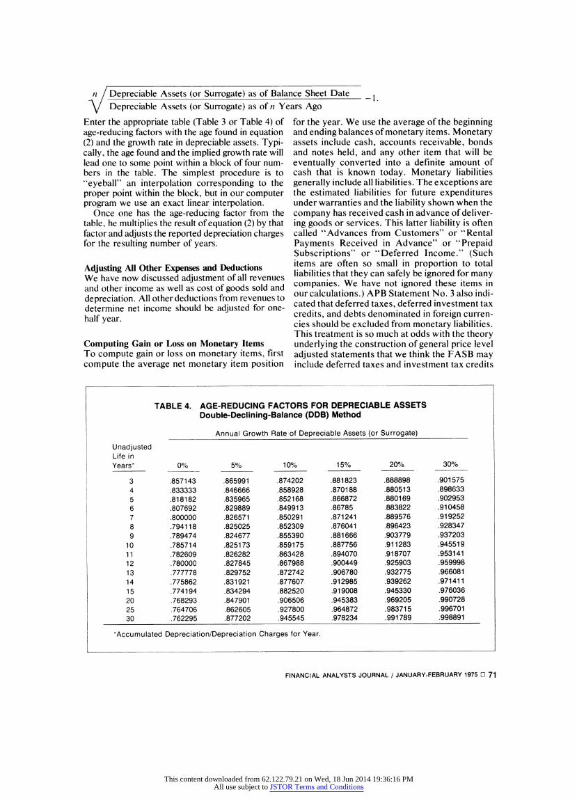
n/ Depreciable Assets (or Surrogate) as of Balance Sheet Date _ _ Depreciable Assets (or Surrogate) as of n Years Ago

Enter the appropriate table (Table 3 or Table 4) of age-reducing factors with the age found in equation (2) and the growth rate in depreciable assets. Typi- cally, the age found and the implied growth rate will lead one to some point within a block of four numbers in the table. The simplest procedure is to "eyeball" an interpolation corresponding to the proper point within the block, but in our computer program we use an exact linear interpolation.

Once one has the age-reducing factor from the table, he multiplies the result of equation (2) by that factor and adjusts the reported depreciation charges for the resulting number of years.

Adjusting All Other Expenses and Deductions We have now discussed adjustment of all revenues and other income as well as cost of goods sold and depreciation. All other deductions from revenues to determine net income should be adjusted for one- half year.

Computing Gain or Loss on Monetary Items To compute gain or loss on monetary items, first compute the average net monetary item position

for the year. We use the average of the beginning and ending balances of monetary items. Monetary assets include cash, accounts receivable, bonds and notes held, and any other item that will be eventually converted into a definite amount of cash that is known today. Monetary liabilities generally include all liabilities. The exceptions are the estimated liabilities for future expenditures under warranties and the liability shown when the company has received cash in advance of deliver- ing goods or services. This latter liability is often called "Advances from Customers" or "Rental Payments Received in Advance" or "Prepaid Subscriptions" or "Deferred Income." (Such items are often so small in proportion to total liabilities that they can safely be ignored for many companies. We have not ignored these items in our calculations.) APB Statement No. 3 also indicated that deferred taxes, deferred investment tax credits, and debts denominated in foreign currencies should be excluded from monetary liabilities. This treatment is so much at odds with the theory underlying the construction of general price level adjusted statements that we think the FASB may include deferred taxes and investment tax credits

TABLE 4. AGE-REDUCING FACTORS FOR DEPRECIABLE ASSETS Double-Declining-Balance (DDB) Method

Annual Growth Rate of Depreciable Assets (or Surrogate)

Unadjusted Life in Years* 0% 5% 10% 15% 20% 30%

3 .857143 .865991 .874202 .881823 .888898 .901575 4 .833333 .846666 .858928 .870188 .880513 .898633 5 .818182 .835965 .852168 .866872 .880169 .902953 6 .807692 .829889 .849913 .86785 .883822 .910458 7 .800000 .826571 .850291 .871241 .889576 .919252 8 .794118 .825025 .852309 .876041 .896423 .928347 9 .789474 .824677 .855390 .881666 .903779 .937203

10 .785714 .825173 .859175 .887756 .911283 .945519 11 .782609 .826282 .863428 .894070 .918707 .953141 12 .780000 .827845 .867988 .900449 .925903 .959998 13 .777778 .829752 .872742 .906780 .932775 .966081 14 .775862 .831921 .877607 .912985 .939262 .971411 15 .774194 .834294 .882520 .919008 .945330 .976036 20 .768293 .847901 .906506 .945383 .969205 .990728 25 .764706 .862605 .927800 .964872 .983715 .996701 30 .762295 .877202 .945545 .978234 .991789 .998891

*Accumulated Depreciation/Depreciation Charges for Year.

FINANCIAL ANALYSTS JOURNAL / JANUARY-FEBRUARY 1975 O 71



as well as items denominated in foreign currencies among monetary items.'1

The major difficulty in practice in considering monetary items is deciding whether or not the asset -Marketable Securities" is a monetary asset. If the marketable securities are bonds, commercial paper, or government notes, then they are monetary. If the marketable securities are equity securities, then they are not monetary. Unfortunately, most firms do not disclose exactly what their marketable securities are.

To compute the average net monetary liability position for the year, add together the monetary liabilities at the beginning of the year and at the end of the year; then subtract the sum of monetary assets at the beginning and the end of the year. Divide the result by two. If positive (as it usually is), the result shows the average net borrowing position of the company during the year; if negative, the average net lending position. The monetary gain for the year is the average riet liability position multiplied by the rate of price change for the year. If the company was a net lender during a year of rising prices, it will have a loss on holdings of monetary items. (Only one of the Dow Jones companies, United Aircraft, and one of the 30 other companies, Merck, show losses on holding of monetary items. On the other hand, several of the banks we have examined show losses on holdings of monetary items, as did Company H shown in Table 6.)

If the company swapped nonmonetary items for monetary items, or vice versa, in large amounts at some time other than near mid-year, then you may want to adjust separately for the resulting monetary gain or loss. If, for example, a company sold a large plant near the end of the year, and the proceeds of the sale are still held in monetary assets, then our averaging process will overstate average monetary assets for the year and understate the gain (or overstate the loss) on holding monetary items.

Preparing the Adjusted Statements The estimated adjustments are now complete. Revenues, other income, and all expenses except cost of goods sold and depreciation are adjusted for one-half year's price change. Gain or loss on monetary items is computed using the entire year's price change. The figures can be summarized as shown in Table 5.

Comments on the Procedure Although the procedure is somewhat complicated to describe, our computer program carries out the estimating procedure for a single company in less

than half a second. It takes us about 30 minutes to compute all the adjustments for a single company by hand.

If the FASB should decide that deferred taxes and items denominated in foreign currencies are not monetary after all, then the gains on monetary items we have reported in the previous section are nearly all overstated. If the FASB condones the ABP Statement No. 3 computation of one-half year's price change, as described in a later section, then our estimates of income are again overstated. Our estimating procedure tries, however, to mirror the logic of the general price level adjustment wherever we can make it do so.

Illustration of the Estimating Procedure

To make the estimating procedure clear and to provide a guide for analysts to follow in preparing their own estimates, we illustrate the estimating procedure in this section. The illustration is for the General Electric (GE) Company's operations for 1973, as reported in the financial statements of its annual report for that year.

Price Index and Rate of Price Change during 1973 The GNP Deflator has the following values for these dates important to the estimating procedure:

Quarterd GN P Deflator (1958 = 100)

4th, 1973 158.93 3rd, 1973 155.67 2nd, 1973 152.61 1st, 1973 149.95 4th, 1972 147.96 4th, 1967" 118.9 3rd, 1967" 117.7

Annual Average

1967'' 117.59 1966'' 113.94

'The GNP Deflator is an average for the quarter. "These are required for the depreciation calculations. 'These are required for the alternative depreciation calculations.

The rate of price increase for the year 1973 is 158.93/147.96 - 1 = 1.0741 - 1 = 7.41 percent. If prices are assumed to have increased uniformly throughout the year, price change during half a year is equal to:"

Price Change for =Vf77i -1 3.64 percent. one-half 1973

72 Q FINANCIAL ANALYSTS JOURNAL / JANUARY-FEBRUARY 1975



Adjustment of Revenues GE's revenues for the year 1973 were $11,759 million (equals "Sales" + "Other income"). Reve- nues are to be adjusted for one-half year. GE's price level adjusted revenues are then

1.0364 x $11,759 million = $12,187 million.

Adjustment of Cost of Goods Sold GE uses LIFO for about 84 per cent of its inventories and uses FIFO for about 16 per cent.12 Historical cost of goods sold was $8,515.2 million. 13

LIFO Adjustment: Under a LIFO cost flow assumption for inventories the purchases that enter cost of goods sold are the last purchases of the year. Total purchases for the year are the cost of goods sold (COGS) plus the increase in inventories for the year.

Purchases = COGS + Increase in Inventories

Purchases = COGS + Closing Inventory (12/3 1)

-Beginning Inventory (1/31)

Purchases = $8,515.2 + $1,986.2 - $1,759.0 = $8,742.4 in millions.

Assuming LIFO, an amount of purchases equal to COGS/Purchases = $8,515.2/8,742.4 = 97.4 per cent of all purchases during the year entered cost of goods sold. These purchases on av,erage occurred 0.974/2 x 12 = 5.844 months before the end of the year. Thus the average dollar of cost of goods sold was dated about July 4, 1973. (De- cember 31 less 5.844 months is about July 4.)

The rate of price change in the last 5.844 months of 1973 was 3.545 per cent. Thus the entire cost of goods sold adjusted for a 3.545 per cent increase in prices is

LIFO COGS - $8,515.2 x 1.03545 = $8,817. Adjusted in millions.

FIFO Adjustment: Under a FIFO cost flow assumption for inventories, the cost of goods sold consists of beginning inventory plus the purchases from the earlier part of the year.

The purchases that enter cost of goods sold for GE in 1973 are the beginning inventory (BI) of $1,759.0 million plus the first $6,756.2 (equals $8,515.2 - $1,759.0 equals COGS - BI) million of purchases for the year. Thus the average dollar of purchases that entered cost of goods sold for GE in 1973 occurred 1/2 x $6,756.2/$8,742.4 x 12 months equals 4.64 months afterJanuary 1, 1973, or about May 20, 1973. The quantity cost of goods sold minus beginning inventory must be adjusted

for 7.36 (equals 12 - 4.64) months-61.3 per cent of a year. The beginning inventory must be adjusted for an entire year.

FIFO COGS = Beginning Inventory Adjusted in x Year's Price Change millions. Adjusted in millions

+ (Cost of Goods Sold - Beginning Inventory)

x Price Change for 0.613 of One Year.

= $1,759.0 x 1.0741

+ $6,756.2 x 1.0449

= $8,948.9.

Combining LIFO and FIFO Adjustments: The adjusted LIFO cost of goods sold was computed to be $8,817.0 and the adjusted FIFO cost of goods sold was computed to be $8,948.7. GE used LIFO for 84 per cent of its inventory and FIFO for 16 per cent. Thus GE's combined-average adjusted cost of goods sold is

COGS =0.84 x $8,817.0 + 0.16 x $8,948.9 Adjusted in millions.

$8,838. 1.

Depreciation GE's depreciation charge for the year 1973 was $334.0 million. The accumulated depreciation at December31, 1973, was $2,559.3 million. Thus, if straight-line depreciation were used, the average dollar's worth of depreciable assets would have been acquired

$2 ,559. 3 = 7.663 years $334.0 per year

before December 31, 1973. GE, however, uses sum-of-the-years'-digits

(SYD) depreciation so that estimate must be reduced somewhat.

To use the SYD adjustment table requires an estimate of GE's annual growth rate in depreciable assets. GE presents the depreciation charges for several past years in its historical summary. 14

The growth rate in depreciation charges provides a surrogate for the growth rate in depreciable assets. Depreciation charges for 1965 (eight years-the closest one shown to 7.663 years -prior to balance sheet date) was $188.4 million. Thus, the depreciation charges increased, on average, at a rate of 7.42 per cent (equals 8 334.0/188.4 - 1) per year between January 1, 1965, and December 31, 1974.




Entering the SYD adjustment table (Table 3) for age 7.663 years and growth rate 7.42 per cent, and interpolating as necessary, yields an adjustment factor of 0.8124. Thus GE's depreciable assets, according to our formula are on average 0.8124 x 7.663 years equals 6.225 years old.

Therefore, depreciation charges must be adjusted for 6.225 years of price change. 6.225 years before December 31, 1973, occurred during the fourth quarter of 1967. Refer to the GNP Deflator for the last two quarters of 1967. We compute that prices increased by 34.9 per cent during the 6.225 years before December 31, 1974.1' The adjusted depreciation charge for GE in 1973 is then

1.349 x $334.0 million equals $450.54 million.

All "Other" Deductions from Income GE's total "other" deductions from income in 1973 were $2,324.7 million. These other deductions consist of interest charges, income taxes, income applicable to minority interests and all operating expenses except cost of goods sold and depreciation.

The other deductions are assumed to be spread evenly throughout the year and are adjusted for one-half year's price change.

Adjusted Other Deductions= $2,324.7 x 1.0364 in millions = $2,409.3.

Computing Gain on Holding of Net Monetary Items GE's monetary items for 1973 were reported as follows: 16

($ in Millions) Dec. 31, 1973 Dec. 31, 1972

Monetary Liabilities All Liabilities ..............,.. $4,901.7 $4,273.8

Monetary Assets Cash, Receivables, Customer Financing, Deferred Taxes, and Recoverable Costs. 2,980.8 2,642.1

Net Monetary Liabilities .$1,920.9 $1 ,63 1.7

The average net monetary liabilities for the year 1973 was $1,776.3 [equals 0.5 x ($1,920.9 + $1,631.7)] million. The price change for the year was 7.41 per cent. Thus GE's gain from being a net debtor during 1973 when prices increased by 7.41 per cent was about 0.0741 x $1,776.3 equals $131 million.

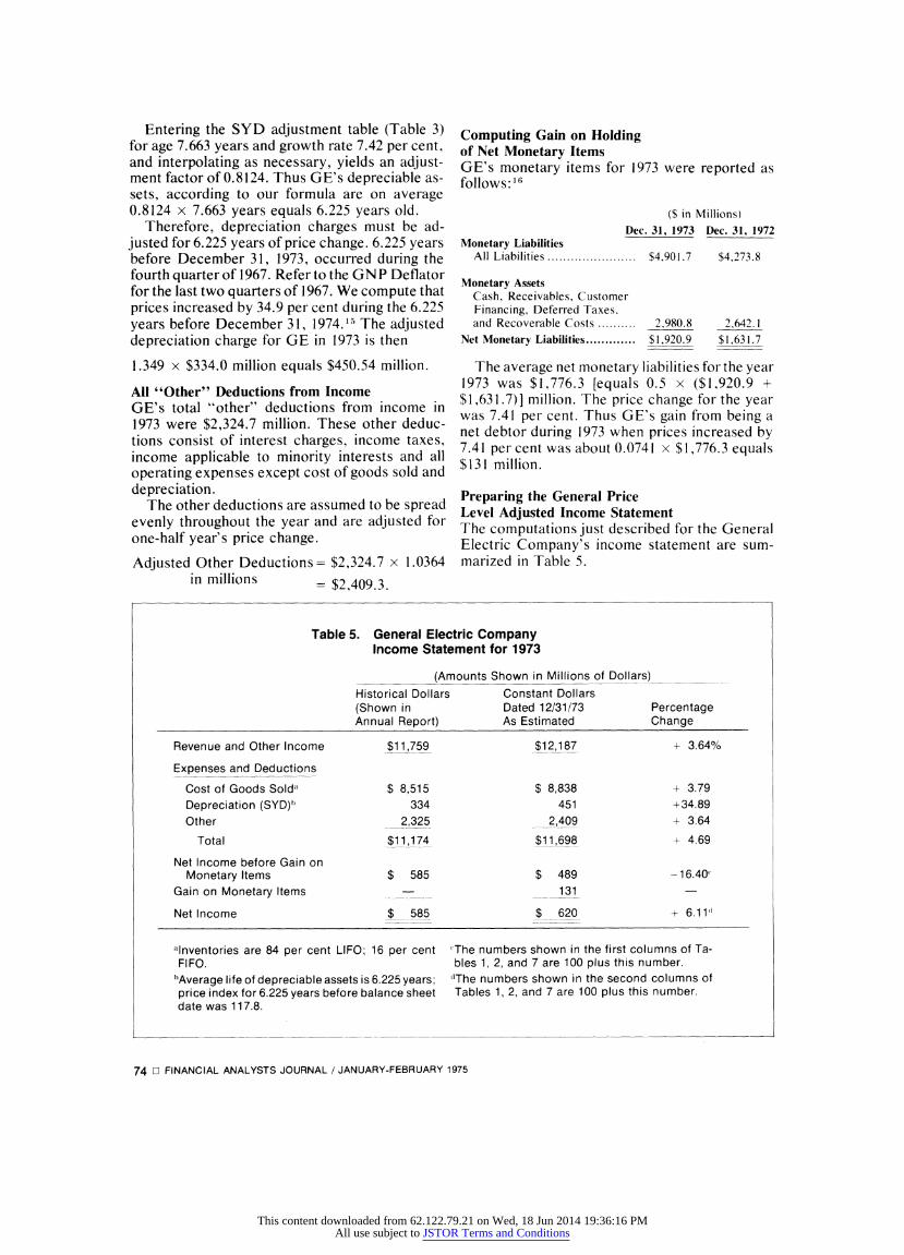
Preparing the General Price Level Adjusted Income Statement The computations just described for the General Electric Company's income statement are summarized in Table 5.

Table 5. General Electric Company Income Statement for 1973

(Amounts Shown in Millions of Dollars)

Historical Dollars Constant Dollars (Shown in Dated 12/31/73 Percentage Annual Report) As Estimated Change

Revenue and Other Income $11,759 $12,187 + 3.64%

Expenses and Deductions

Cost of Goods Solda $ 8,515 $ 8,838 + 3.79

Depreciation (SYD)') 334 451 +34.89

Other _2,325 __ 2,409 + 3.64

Total $11,174 $11,698 + 4.69

Net Income before Gain on Monetary Items $ 585 $ 489 -16.40t

Gain on Monetary Items 131

Net Income $ 585 $ 620 + 6.11'

alnventories are 84 per cent LIFO; 16 per cent (The numbers shown in the first columns of Ta- FIFO. bles 1, 2, and 7 are 100 plus this number.

"Average life of depreciable assets is 6.225 years; 'The numbers shown in the second columns of price index for 6.225 years before balance sheet Tables 1, 2, and 7 are 100 plus this number. date was 117.8.

74 El FINANCIAL ANALYSTS JOURNAL / JANUARY-FEBRUARY 1975



How Accurate Is The Estimating Procedure?

The previous sections have presented procedures for estimating general price level adjustments to reported income and have shown the results of those procedures for 1973 operations of 60 major corporations. We have suggested that analysts can use these procedures for preparing general price level adjustments for companies of interest to them. How similar are the results using these procedures to the results that would be reported by major companies if general price level adjusted statements were required?17 We attempt to an- swer that question, insofar as we can, in this section.

We have partial, reported ("actual") general price level adjusted accounting figures for three companies on a current basis-Gulf Oil Corpora- tion, Shell Oil Company, and Indiana Telephone Corporation. A fourth company, called Company R, helped us assess the accuracy of our procedures on a confidential basis. In addition, the AICPA commissioned a study of general price level accounting in 1968-69.18 The AICPA made available to us the financial statements for a dozen or so companies in that study. Those data contain three companies for which we can apply our estimating procedures. (The others cannot be tested because some vital information-such as the start of the year balance sheet-was not given to us.) These are real companies, but their names were withheld. Next the AICPA published results for a fictitious XYZ Company in APB Statement No. 3 that explains the general price level restatement procedure. Finally, one standard accounting reference book contains a chapter on inflation accounting which shows a comprehensive example of general price level adjustments for another fictitious company, Demonstrator Corporation. Table 6 presents partial comparisons of our results and reported figures for these ten companies. The results are partial in the sense that some of the real companies made available (published) only parts of their general price level adjusted financial statements. We compare our numbers with the published excerpts.

You can judge for yourself the results shown in Table 6. Our estimated bottom line figures-net income-for Gulf and Company R are within six per cent of the companies' numbers. For Shell we are off by 10 per cent. Indiana Telephone does not report gains on monetary items as suggested in APB Statement No. 3, but our estimates of their net income before gain on monetary items is within five per cent of the reported figure.

At first glance the following may appear puz-

zling. For some companies (such as Company P of the Rosenfield Study) the estimates of the income items are in error by substantially more than the components of income are in error. Recall, however, that the denominator for each error calculation is the reported figure of that financial statement item and keep in mind that net incomes are typically less than fi've per cent of revenues or cost of goods sold. Errors in estimates of the same absolute dollar amounts are, then, a much larger percentage of net income than they are of total revenues or of cost of goods sold.

For the fictitious AICPA example (XYZ Company) we do well for 1967, but poorly for 1968. The XYZ Company comparisons should not be given much weight because the GNP De- flator Series has been changed since the 1968 publication date of Statement No. 3. That is, the AICPA used numbers for the GNP Deflator Series different from the ones now considered official.

Furthermore, the assumed 1968 operations of XYZ Company resulted in a drastic decline in income from 1967. Whereas revenues for 1968 were about 10 per cent less than in 1967, income was about 75 per cent less. When computing the deviation of our estimate of net income from the reported result, we divide by reported net income, which is small for 1968. When the denominator is small, the resulting percentage can be large even when the absolute deviation is not, as suggested in our comment on International Harvester and United Aircraft in an earlier section.

The large difference between our estimate for gain on monetary items for XYZ in 1968 and the reported figure is caused by XYZ's selling a nonmonetary asset on December 31, 1968. The cash realized from that sale is larger than the total amount of net monetary liabilities. Our standard procedure assumes that all inflows of cash occur evenly throughout the year; that assumption substantially reduced both the estimated average net monetary liability and the gain on monetary items for the year from that reported by the XYZ Com- pany. Since the nonmonetary asset sold was converted into the monetary asset cash on December 31, 1968, this transaction did not affect reported gain on monetary items at all. When we account separately for this one transaction, the error in reporting gain on monetary items for XYZ Com- pany in 1968 is reduced from 45 per cent to less than 20 per cent.

The estimates for the Demonstrator Corpora- tion are gratifyingly accurate. The primary cause of the over adjustments for ordinary income items is the same as the cause of our other over adjust-




Table 6. Percentages by Which the Davidson-Weil Estimates Deviate from the Reported General Price Level Adjusted Items

[For each item, the number shown is the Davidson-Weil estimate divided by the general price level adjusted item as reported (by the Company or by the AICPA) minus one:

Number shown=DW/Reported- 1. A positive number indicates an overestimate by Davidson-Weil; a negative number, an underestimate.]

Company and Year AICPA-Rosenfield Study AICPA Demon-

General Price Level Gulf Shell Company Indiana XYZ Company strator Adjusted Financial Oil Oil R Telephone Co. H Co. J Co. P Company Statement Item (1973) (1973)" (1973), (1973)1 (1968)1 (1968)t (1968)t (1967)' (1968)' (1960)

Revenues and Other Income 3.63% 0.68% 9.00% 0.72% 0.05% 0.25% 0.13% 1.38% 0.35%

Cost of Goods Sold 0.02 0.79 0.11 -1.78 0.07 0.75 0.18

Depreciationh 5.93% 18.74 6.46 6.33 2.99 3.45 2.62 -4.29 0.41

Other Expenses and Deductions 0.62 8.08 0.94 -0.29 0.31 -0.23 6.30 0.03

INCOME BEFORE GAIN OR LOSS ON MONETARY ITEMS - 9.97 4.75 10.77 -1.43 24.67 -3.41 60.76i 5.01

Gain or Loss on Monetary Items 5.80 11.17i -6.08 -53.33 -1.00 -45.12i -4.21

NET INCOME 5.23, -10.13 - 5.78 - 3.03 -2.46 7.33 -3.38 30.53 4.62

*Not reported by the Company. `Indiana Telephone Company has no cost of goods sold. ***Not computed by Indiana Telephone in accordance with APB Statement No. 3.

Footnotes to Table 6

a. Gulf Oil Corporation, The Orange Disc, July-August 1974, p. 31.

b. Shell Oil Company, Shell Shareholder News, June1974, p. 1.

c. From the company itself on a confidential basis. The company reports that its depreciable assets are only about half as old as our computation (Accumulated Depreciation/Depreciation for the Year) indicates.

d. Indiana Telephone Corporation, Annual Report for 1973.

e. AICPA data compiled by Paul Rosenfield. See Paul Rosenfield, "Accounting for Inflation-A Field Test," The Journal of Accountancy, June 1969, pp. 45-50.

f. American Institute of Certified Public Accountants, Ac- counting Principles Board Statement No. 3, "Financial

Statements Restated for General-Price Changes," June 1969, Exhibit B.R-3 (12/31/68).

g. Robert T. Sprouse, "Adjustments for Changing Prices," in S. Davidson (editor), Handbook of Modern Accounting, New York: McGraw-Hill Book Co., 1970, Chapter 30, page 26.

h. Straight-line method is used by all companies. i. See text for explanation of these large deviations. The

Davidson-Weil estimates are off by only $95,000 for income items and less than $40,000 for gain on monetary items. Revenues for the year were $27 million.

j. DW overstate the amount of the loss on monetary items. k. We include marketable securities in monetary items; it

is not clear what Gulf does.

ments, which is explained next. The major cause of the difference between the

results of our estimating procedure and the published company results, as far as we can tell, comes from the adjustment for revenues and other items spread evenly throughout the calendar year. APB Statement No. 3 suggests that the adjustment factor be:

GNP Deflator (4th Quarter) GNP Deflator (Average for Year)

But the GNP Deflator (4th Quarter) is the average for the fourth quarter (about November 15), not the price level as of December 31. Hence, the AICPA procedure adjusts items "spread fairly evenly throughout the year" on average from about June 30 to about November 15-four and one-half months. The adjustment is supposed to be for six months, a time period one-third longer.19 We believe the AICPA procedure under adjusts for the items spread fairly evenly throughout the year. In our own procedures we use the factor




GNP Deflator (4th Quarter This Year) GNP Deflator (4th Quarter Last Year)

for items requiring, on average, one-half year's adjustment. We suggest that a reasonable approximation to this geometric mean i

( GNP Deflator (4th Quarter This Year) A

O GNP Deflator (4th Quarter Last Year)

At any rate, our adjustments for a half year are always larger than those found by following the AICPA procedures. We surmise, but cannot be sure, that the four real companies used in our comparisons with 1973 data have followed the AICPA method of adjusting for four and one-half months on average, rather than the six months we suggest. We know that Demonstrator Corpora- tion's adjustments for items spread evenly throughout the year were made using the four and one-half month AICPA technique. In general, during times of increasing prices, the result of using only four and one-half rather than six months for adjusting items spread fairly evenly throughout the year is to underestimate general price level adjusted profits. The items spread evenly throughout the year are (1) nearly all revenues and (2) many expenses. Since the sum of ".nearly all revenues" exceeds the sum of "many expenses" for almost all companies, the excess-a partial gross margin-is understated.

Once the FASB makes official its standards for general price level adjustments, those who want to estimate results will want to pay careful attention to the half-year adjustment suggested (or required) and to build an analogous computation into the estimating procedure. We think we have used the most logical procedure, but we can change it if, as has happened before, the FASB does not agree with us about what is logical.

All the companies for which we can assess the accuracy of our methods use straight-line depreciation. We cannot, however, test the accuracy of our methods for firms using accelerated depreciation until some such firms publish their general price level adjusted depreciation figures.

Some Implications

Data reported previously on the effects of general price level adjustments on income have been fragmentary, and most relate to periods when the rate of price level change was more modest. Our results for the 60 corporations were summarized in the first section. At that point we noted that (1) effects differ substantially among firms, (2) in-

come before recognizing monetary gains is reduced for all firms and substantially reduced for many, and (3) adjusted net income (including monetary gains) is surprisingly high (to us, at least) in relation to reported net income.

Some more general implications suggested by consideration of the special factors involved, as well as by analysis of our data, are spelled out in the following paragraphs.

Rapidly Growing vs. Slowly Growing Companies General price level adjustments tend to affect rapidly growing companies less than slowly growing companies. Put another way, rapidly growing companies have, on the average, newer plants and the upward adjustment of depreciation expense is lower for them than for most slowly growing companies. This effect is compounded if, as is likely to be the case, the rapidly growing company has a higher portion of its capitalization made up of debt. In that case, it will have more monetary gains to report.

For believers in the desirability of economic growth, general price level adjusted statements may have a serendipitous effect. The more rapidly growing companies are likely to show an im- proved earnings picture relative to slower growing companies. Whether one believes this will affect the cost of capital to them depends on whether one believes in the efficiency of capital markets.

The Importance of Monetary Gains Monetary gains will be a significant factor in the adjusted net income of many firms. For the Dow 30 companies, they raised the median firm from 69 per cent of reported net income to 92 per cent (see Table I) and for the other 30, monetary gains raised median net income from 64 per cent of reported income to 99? per cent of it - suggest- ing that the other 30 have a higher average debt ratio than the Dow 30.

Clearly, the higher the debt ratio, the greater will be the significance of monetary gains. But these monetary gains do not produce cash inflows for the firm; they show the reduced economic significance of outflows that will have to be made later. In the meanwhile interest payments on the debt must be made. Recognition of monetary gains in adjusted income may enable a company to show adjusted profits even though its cash position is deteriorating. It has been suggested that with enough debt outstanding a firm can report profits (on a general price level adjusted basis, including monetary gains) right up to the time it goes bankrupt.




Effects of More Rapid Inflation A more rapid rate of inflation will in almost all cases reduce adjusted income before monetary gains as a percentage of reported income. The effects of more rapid inflation on adjusted net income (including monetary gains) are more dif- ficult to predict. Clearly it depends on the relative importance of greater monetary gains compared to higher cost of goods sold and depreciation expense figures.

To help assess the significance of more rapid inflation, we repeated the analysis of the 1973 operations of the Dow companies assuming a general price level increase of 12 per cent rather than the 7.4 per cent actually experienced. (Twelve per cent is the rate of general price level increase suggested by many economists as the one that will be reported for 1974 when all the returns are in.) The results of assuming the 12 per cent inflation rate are shown in Table 7.

Perhaps the best way to consider this effect is to present the quartile distributions of general price level adjusted income as a percentage of reported income for two inflation rates for the Dow companies. They are:

General Price Level Adjusted Income as a Percentage of

Reported Income

Actual 7.4% Assuming Inflation 12% Inflation

Net Income before Monetary Gains

Lowest Quartile 10- 34%X (-37)- 15% Second Quartile 34- 68% 15 - 57% Third Quartile 70- 80%c 61 - 75% Highest Quartile 80- 87%1 75 - 81%

Net Income Lowest Quartile 18- 81%7 (-17)- 79% Second Quartile 81- 92% 79 - 93% Third Quartile 92- 98% 95 -104% Highest Quartile 98-153% 104 -195%

Net income before monetary gains is uniformly lower at the higher inflation rate. Adjusted net incomes with a 12 per cent inflation show a much broader range than with a 7.4 per cent inflation. Some firms report worse results, but more show better results. For example, seven of the 30 companies show higher adjusted net income than reported income with a 7.4 per cent inflation rate. That number grows to eleven of 30 with a 12 per cent inflation rate.

The results with higher inflation rates em- phasize again the differential effects among firms of general price level adjustments and the great significance of monetary gains and losses.

Table 7. Dow Jones Companies Adjusted 1973 Income as a Percentage of Reported Income, IF price increase during 1973 had been 12 per cent

Adjusted Net Adjusted Net Income before Income, including Gain on Monetary Gain on Monetary Items as a O/o of Items, as a % of Reported Net Reported Net

Company Income Income

Allied Chemical 8% 57% Alcoa 18 128 American Brands 24 91 American Can 5 88 AT&T 75 195 Anaconda 69 97 Bethlehem steel 35 98 Chrysler -19 85 du Pont 63 63 Eastman Kodak 81 87 Esmark Inc. 3 64 Exxon 76 101 General Electric 80 116 General Foods 62 104 General Motors 56 60 Goodyear 35 103 International

Harvester -37 53 International

Nickel 72 112 International

Paper 61 91 Johns-Manville 81 103 Owens-lllinois 57 105 Procter & Gamble 80 99 Sears Roebuck 68 76 Standard Oil of

California 80 95 Texaco 77 104 Union Carbide 54 85 United Aircraft 0 -17 U.S. Steel 15 79 Westinghouse 71 130 Woolworth 9 93

Median 57 to 61 93 to 95

A negative number indicates a loss equal in amount to the indicated percentage of reported income.

Effects of More Extensive Lease Capitalization One of the topics currently being considered by the FASB is more extensive lease capitalization. If this occurs, there will be an increase in reported long-lived assets and also long-term debt in the amount of the present value of the lease commit- ments. Both the dollar difference between reported and adjusted depreciation and the amount of monetary gains would be increased by such broader capitalization. In the typical case, the increase in monetary gain is likely to exceed -

usually by a substantial amount for a growing firm -the additional depreciation charges. The dif-

ference between the two depends on the inflation

78 El FINANCIAL ANALYSTS JOURNAL / JANUARY-FEBRUARY 1975



rate this year compared to that of earlier years, the length of the leases, and where in the life cycle of the leases this year falls.

If general price level adjusted statements are required, precisely those growing companies that will have their reported earnings most adversely affected by lease capitalization will have the greatest boost to general price level adjusted earnings from that capitalization. Perhaps this consideration will diminish some of the opposition to broader lease capitalization.

APPENDIX:

Accounting for Changing Prices

This appendix briefly describes methods that have been suggested for accounting for changing prices. The methods are illustrated in Tables 8 and 9 for simple situations. Even though the ex- amples are simplified, they incorporate virtually all of the complications and issues of inflation accounting.

There are essentially two different kinds of accounting for changing prices: current value accounting and constant dollar accounting. In the following description, three methods are presented: current value accounting, general price level adjusted (constant dollar) accounting, and (a synthesis of these two kinds) current value accounting combined with general price level adjustments. The first and the last of these [illustrated in columns (2) and (4) of Tables 8 and 9] are similar methods because the balance sheet totals are identical. Reported net income differs, however, and the balance sheet items are clas- sified in different ways.

Revenues, Inventory, Cost of Goods Sold and Holding Gains or Losses Table 8 shows transactions for a hypothetical company for a year in which the general price level increased by 32 per cent (20 per cent in the first six months and 10 per cent in the second six months - 1.20 x 1.10 = 1.32). The fair market value of inventory units (widules) was $50 per unit on January 1, $80 on June 30, and $90 on De- cember 31. (It is not at all unusual, of course, for some specific price changes to differ substantially from the change in the general price level. Realis- tic cases of even more substantial differences than those used in the example are easily found.)

The company starts the year with $ 100 cash and $100 of contributed capital, as shown in the

January 1 balance sheet. The company buys two widules on January 1 for $50 each and sells one on June 30 for $120.

Historical Dollar Generally Accepted Account- ing Principles: Column (1) shows how these transactions are accounted for under generally accepted accounting principles (GAAP). Revenues are $120. cost of goods sold is $50, and net income is $70.

Current Value Accounting: Column (2) shows how the transactions would be accounted for under current value or replacement cost accounting. Revenues are still $120. The cost of the unit sold, at the time it was sold, is $80, so the operating income is $40. In addition, there is a realized holding gain on the item sold of $30 (equal to current value at time of sale of $80 less acquisition cost of $50). Furthermore, there is an unrealized holding gain of $40 (equal to current value of $90 at end of year less acquisition cost of $50). Thus net income is $110 (equals $40 + $30 + $40). The December 31 balance sheet shows all assets and liabilities at current values as of December 31.

General Price Level Adjusted Accounting Based on Historical Costs: Column (3) shows general price level adjusted accounting as described in APB Statement No. 3 and in this article. All costs are historical, but financial statement data are restated to dollars of constant purchasing power. In the illustration, the dollar of constant purchasing power are December 31 dollars.

Revenues of $120 realized on June 30 are the equivalent of $132 of December 31 purchasing power; prices increased by 10 per cent between June 30 and December 31 so that it takes $132 in December to buy the same general market basket (as represented by the GNP Deflator) that could have been bought on June 30 for $120.

The cost of goods sold of $50 in historical dollars is reported as $66 (equals 1.32 x $50) in terms of December 31 purchasing power.

Since the company held cash ($120) from June 30 through December 31, when the purchasing power of the dollar declined by 10 per cent, there is a loss on holdings of monetary items of $12 (equals 0.10 x $120).

The balance sheet shows the historical cost of inventory restated to dollars dated December 31. The amount of capital contributed by owners was $100 in terms of January 1 purchasing power. This amount is equivalent to $132 of December 31 purchasing power since prices increased by 32 per cent during the year. Hence contributed capital is shown on the balance sheet in terms of December 31 purchasing power as $132. The retained earn-




Table 8. Traditional Accounting Compared with Current Value and Constant-Dollar Accounting

Balance Sheet as of January 1, 19XX Cash: $100 Contributed Capital: $100

Date January 1, 19XX June 30, 19XX December 31, 19XX

GNP Deflator 100 - (20% increase)-- 120 - (10% increase)-- 132 Cost of one Widule $50 $80 $90 Transaction Buy 2 widules Sell 1 widule Close books and

at $50 each, $100. for $120. prepare statements.

Historical Dollars Constant Dollars Dated 12/31/XX

Cost Basis Acquisition Replacement Acquisition Replacement Usual Name GAAP Current Value GPLA Cur. Val.&GPLA

Income Statement (1) (2) (3) (4) Revenues $120 $120 $132a $132a Cost of Goods Sold 50 80 66b 88e

Operating Income $ 70 $ 40 $ 66 $ 44 Realized Holding Gains 30d 22e Gain (Loss) on Monetary Items - (1 2)f (1 2)f

Realized Income $ 70 $ 70 $ 54 $ 54 Unrealized Holding Gains 40g 24h

Net Income $ 70 $110 $ 54 $ 78

Balance Sheet Assets

Cash $120 $120 $120 $120 Inventory 50 90 66h 90

Total Assets $170 $210 $186 $210

Equities Contributed Capital $100 $100 $132 $132 Retained Earnings 70 70 54 54 Unrealized Holding Gains 40 24

Total Equities $170 $210 $186 $210

(1) Traditional (2) Easy to Explain / Hard to Audit (3) Hard to Explain / Easy to Audit (4) Hard to Explain / Hard to Audit a. $120x1.10 b. $50x1.32 c. $80x1.10 d. $80-$50 e. ($80-1.20x$50)xl.10 f. $120x(-10%) g. $90-$50 h. $90-($50x1.32)

ings amount shown on the balance sheet is trans- ferred from the income statement.

Current Values Adjusted for General Price Level Changes: Column (4) of Table 8 shows the accounting when the principles of current value accounting are combined with the principles of stat- ing all amounts in constant dollars. This approach has received acceptance among many theorists as the best possible approach, but is not likely to be required in the forseeable future.

Revenues are translated to end of year dollars as in Column (3). Cost of goods sold in current values is $80 as of June 30. But these are dollars of June 30 purchasing power. Translated to dollars of December 31 purchasing power, cost of goods sold is 10 per cent more than $80, or $88.

The realized holding gain is measured as follows. In terms of June 30 purchasing power, the holding gain is current value on June 30 less acquisition cost translated into dollars of June 30




purchasing power. The acquisition cost of $50 on January 1 is the equivalent of $60 (equals 1.20 x $50) of June 30 purchasing power. Hence the realized holding gain is $80 (current value as of June 30) less $60 (cost in June 30 dollars), or $20. This holding gain of $20 is measured in dollars of June 30 purchasing power and represents $22 (equals 1. 10 x $20) of December 31 purchasing power.

The unrealized holding gain is somewhat easier to compute: The current value of one widule on December 31 is $90. It cost $50 on January 1, which is equivalent to $66 (equals 1.32 x $50) of December 31 purchasing power. The unrealized holding gain is $24 (equals $90 - $66).

Cash was held during the second half of the year when prices declined by 10 per cent so there is a loss on holdings of monetary items of $12, calculated as before.

The balance sheet shows inventory at current values as of December 31 and the amount of contributed capital in terms of December 31 purchasing power. Notice that the balance sheet totals in Column (4) are the same as in Column (2). This is no coincidence. The only basic difference between the two approaches to current value accounting is that net income is reported differently. When the effects of changing prices are incorpo- rated into current value accounting, we get a sep- aration of real holding gains from nominal holding gains. The $32 difference between the net incomes reported in Columns (2) and (4) reflects the fact that the contributed capital in December 31 dollars is exactly $32 more than contributed capital in January 1 purchasing power. That $32 is not reported as income in price level adjusted current value accounting but is in historical dollar current value accounting.

Long-Lived Assets and Accounting for Changing Prices Accounting for long-lived assets and depreciation in schemes designed to reflect changing prices requires some special techniques. These are explained in this section and in Table 9. The assumptions for the illustration are spelled out at the head of Table 9.

Current Value Accounting: At the start of 19X4, the current value of the asset is $20,000 and it is 30 per cent "gone," so accumulated depreciation must be $6,000 and the book value must be $14,000. During the year 10 per cent of the asset's cost is allocated to depreciation charges for the year. The asset's average cost during the year is $22,500 equals ($20,000 + $25,000)/2. Thus the depreciation charge for the year, based on 10 per

cent of "cost," is $2,250. During the year, however, the current value of

a similar, but new, asset increased from $20,000 to $25,000. Thus the owner of the asset has a holding gain. The gain on an unused asset would have been $5,000 but, on average, our asset was only 65 per cent new during the year. (It was 70 per cent new at the start of the year and 60 per cent new at the end of the year.) Thus our holding gain is only 65 per cent of $5,000, or $3,250.21

General Price Level Adjustments for Long-lived Assets: Column (3) of Table 9 shows the accounting for the long-lived asset with general price level adjustments. During the four years since the asset was acquired, the general price level increased by 40 per cent. The December 31 balance sheet would show the asset's cost at $14,000, which is equal to the original cost of $10,000 restated to December 31, 19X4, dollars. At the start of the year the asset of 30 per cent is gone so the book value at the start of the year is 0.70 x $14,000 equals $9,800 of December 31, 19X4, purchasing power.

Depreciation charges for the year are 10 per cent of cost stated in December 31 dollars, or $1,400. As of the end of the year, the asset is 60 per cent gone.

Of all the adjustments in generally price level accounting, the depreciation adjustment is likely to show the largest change from the traditional statements. Furthermore, it is likely to be the least meaningful. Only when the current value, or replacement cost, of assets similar to the ones being depreciated have changed as the GNP De- flator has changed will the adjustment reflect re- levant information.

Current Value Adjusted for General Price Level Changes: Column (4) of Table 9 shows the accounting when the techniques of Column (2) for current values and Column (3) for general price level adjustments are combined.

The current value of the asset at the beginning of 19X4 was $20,000 but that amount is equal to $22,000 of December 13, 19X4, purchasing power. Since the asset is 30 per cent gone at the start of 19X4, its book value is $15,400. or 70 per cent of $22,000, in December 31 purchasing power.

The depreciation charge for the year is 10 per cent of the average value of the new asset expressed in December 31, 19X4, dollars. The average value during 19X4 is $23,500 [equals (1.10 x $20,000 + $25,000)/2]. Hence the depreciation charge for the year is $2,350.

The holding gain for the year is computed as

FINANCIAL ANALYSTS JOURNAL / JANUARY-FEBRUARY 1975 EJ 81



Table 9. Illustration of Depreciation Computations, General Price Level Adjustments and Related Holding Gains for Long-Lived Assets

Assumptions. 1. Machine purchased new on 1/1/X1 for 5. GNP Deflator increased by 10 per cent be-

$10,000. tween 1/1/X4 and 12/31/X4. 2. Machine lasts 10 years and has zero salvage 6. New Machine of exactly the same type as the

value at retirement. one purchased in (1) costs $20,000 on 1/1/X4 3. Depreciation computed on a straight-line ba- and $25,000 on 12131/X4.

sis at 10 per cent of cost per year. 7. Used machine just like the one purchased in 4. GNP Deflator increased by 40 per cent be- (1) costs $14,000 on 1/1/X4 and $15,000 on

tween 1/1/X1 and 12/31/X4. 12/31/X4.

Constant Dollars Historical Dollars Dated 12/31/X4

Current Current Value

GAAP Value GPLA & GPLA

Balance Sheet, 1/1/X4 (1) (2) (3) (4) Asset "Cost" $10,000 $20,000 $1 4,000a $22,000h

Less Accumulated Depreciation(' (3,000) (6,000) (4,200) (6,600) Book Value (30% gone) $ 7,000 $14,000 $ 9,800 $15,400

Income Statement for 19X4 Depreciation

(10% of Average "Cost" During Year) (1,000) (2,250)(' (1,400)c (2,350)f

Holding Gain 3,2509 1,950h

Balance Sheet. 12/31/X4 Book Value (40% gone) $ 6,000 $15,000 $ 8,400 $15,000 Asset "Cost"i $10,000 $25,000 $14,000 $25,000

Footnotes for Table 9

a$1 0,000 x1.40. 9Gain on "unused" asset during year is $5,000. b$20,000 x 1.1 0. On average, our asset was 65 per cent new during "Asset is 30 per cent gone at January 1; 30 per the year; 0.65x5,000=$3,250. cent of "Cost." hGain on "unused" asset during year in constant d10 per cent of average cost of new asset during dollars dated December 31, 19X4, is $3,000=

d1 er cent of average cost of new asset during $25,000-1.1Ox$20,000. On average, our asset year; 0.1 0x ($20,000+ $25,000)/2=$2,250 $5Q0 .0x2,0. naeae u se year;p 0'nof(adju $25d000)/2f$2,250. was 65 per cent new during the year; 0.65x elO per cent of adjusted cost of $14,000. $3,000=$1,950. flO per cent of average cost [=0.5x($22,000 iNote that 40 per cent of "cost" is the book value +$25,000)] of new asset expressed in dollars shown just above. dated December 31, 19X4.

follows. An unused asset increased in value by $3,000 (equals $25,000 - 1.10 x $20,000) of De- cember 31 purchasing power. On average our asset was 65 per cent unused during 19X4, so the holding gain is 65 per cent of $3,000, or $1,950.0.22

It is not coincidence that the net book values of the asset to be shown on the December 31 balance sheet is the same in Columns (2) and (4).

Summary

Columns (1) of Tables 8 and 9 show generally accepted accounting principles. Columns (2) show current value accounting. Current value accounting is easy to explain but hard to audit. It requires estimates of the current values of all assets and liabilities. More often than not, prices for

82 E FINANCIAL ANALYSTS JOURNAL / JANUARY-FEBRUARY 1975



"(used" assets are hard to get. Auditors would be required to make substantial judgmental decisions in implementing current value accounting. But we live in a litigious age and auditors are reluctant to exercise judgment in such situations because, oc- casionally, judgments would have to be published that could not be well documented and might lead to lawsuits if the judgment was proved wrong by subsequent events.

Other problems of current value accounting have not yet been settled by theorists. When there is a "bid-asked" spread for an asset - the replacement cost is higher than the current selling price (or net realizable value) - which of these numbers should be used? Those who believe in replacement costs are called "entry value" theorists and those who believe in net realizable values are called "exit value" theorists.

Columns (3) show historical costs adjusted for general price level changes. This is the treatment that is likely to be required. It is in many ways a meaningless, and sometimes misleading, treatment.23 But it is easy to audit and is objective. Two auditors given the same historical records and the same data for the GNP Deflator are likely to derive the same general price level adjusted statements.

In our opinion, the gain or loss on holdings of monetary items is the part of general price level adjusted accounting that results in adjustments that are both large and meaningful.24 The interest expense reported in traditional accounting statements is the actual interest paid (adjusted, of course, for opening and closing balances of interest payable). The interest paid depends upon the interest rate negotiated at the time of a loan. That interest rate, in turn, depends in part on the lender's and borrower's forecasts of the anticipated rate of inflation. Thus the borrower is charged in the traditional statements for inflation expected by the borrower and the lender. The holding gain from monetary liabilities in a time of rising prices in a real sense deducts from interest expense the gain from being a debtor during the inflation that both parties to the loan expected. After the fact, who benefited, the borrower or the lender, really depends on whether the actual rate of price increase during the period of the loan differed from the rate anticipated by both parties to the loan at the time the loan was made. If the actual rate of price increase turns out to have been less than the anticipated rate, then the lender benefited. If the actual rate turns out to have been greater than the anticipated rate, then the borrower benefited.

Otherwise, in our opinion, general price level adjustments do not convey much useful information. Still, these are what we think are going to be

required and the analyst will have to understand both their meaning and their limitations.

The accounting shown in Columns (4) is, in our opinion, the best solution to the problem of accounting for changing prices. It incorporates both current values and holding gains and losses on all assets including the recognition of gain or loss on holdings of monetary items. It is, however, both hard to explain and hard to audit and is unlikely to receive much acceptance in practice. .

Footnotes

'See Financial Accounting Standards Board discussion memorandum, " Reporting the Effects of General Price-Level Changes in Financial Statements," dated February 15, 1974, and Provisional Statement of Standard Accounting Practice 1 of the Accounting Standards Steering Committee [of the several accounting institutes of the United Kingdom] titled "Ac- counting for Changes in the Purchasing Power of Money,- dated June 1974.

2The 30 ''other" companies were almost entirely selected on a random basis from the roster of companies in the Fortuine 500 whose annual reports were readily available to us. This helps explain the large number of Chicago-based and southeastern companies. Shell Oil and Gulf Oil, however, were included because the accuracy tests described in a later section were possible for them.

The percentage figures shown for most of the companies in this list of "other" companies were derived by hand calculations, rather than from the computer program used for the companies on the Dow list. Our checks indicate that the different calculation methods produce no significant difference in results.

3This long title is used in the FASB discussion memorandum of February 15, 1974, on the subject. APB Statement No. 3 indicates a preference for the briefer "general price level gain or loss." The FASB uses that title in the illustration in the discussion memorandum, but it also uses the phrase "purchasing power gain or loss" that was recommended in Accounting Research Study No. 6. We have chosen to use the simpler, and in our opinion, more meaningful, phrase "monetary gain or loss.-"

4The three areas are: (1) the method of calculating the adjustment factor for revenues and other items spread fairly evenly throughout the year; (2) treating deferred taxes and deferred investment credit as monetary items, and (3) treating foreign debt as a monetary item. Each of the items is discussed in later sections.

5We are not the first to challenge the validity of the naive view that a constant adjustment factor will suffice. See Russell J. Petersen, " Interindustry Estimation of General Price-Level Impact on Financial Information," The Accounting Review, 48, 1 (January 1973), pp. 34-43.

6These numbers only approximate the actual GN P Deflator for those two quarters.

7A more accurate computation is to use

A/1.12 - 1 = (1.12) 1/2 - 1 = 1.0583 - 1 = 5.83 percent

as the average of price change for a half-year when prices went up by 12 per cent for the whole year. This more exact computation, and the analogous ones for other fractions of a year, can be done if you have a calculator or computer that raises numbers to fractional powers. We use the simpler, but less exact, procedure explained in the text for hand calculations but our computer program uses the more accurate method described in this footnote and the next.

The AICPA in APB Statement No. 3 actually recommends a different procedure, explained below. It is so clearly inferior




to both the methods described here that we are hopeful the FASB will use one or the other of these two.

'The more accurate computation, analogous to the one described in footnote 7, is to use

(1.12) 0.62 - 1 = 7.28 per cent

as the rate of change in prices for 62 per cent of a year during which prices increased by 12 per cent.

9To see how this computation works, consider an asset costing $10,000 on which accumulated depreciation is $3,000 at year-end and for which annual straight-line depreciation charges are $1,000. We know that the asset has a 10-year life ($10,000/$ 1,000 per year) and that the asset is 30 per cent gone as of the end of the year ($3,000/$10,000). Thus the asset is 30 per cent of 10 years, or three years old, at the end of the year.

10We have counted these items among monetary items except in some of our "calibrating" calculations where the company has reported a different treatment.

11 A simpler computation of the price change during one-half year is 1/2 x 7.41 per cent = 3.705 per cent. (1.03705)2 is, however, greater than 1.0741. Using one-half the year's price change (3.705 per cent) rather than the price change for one- half a year (3.64 per cent) will bias the computations by assuming, in effect, that prices increased more rapidly in the second half of the year than in the first half. Such a bias results in slight over-adjustments.

12This information is given on page 36 in the notes to GE's 1973 annual report. That annual report is reproduced and annotated in Accounting: The Language of Business, Sidney Davidson, James S. Schindler, and Roman L. Weil, Glen Ridge, New Jersey (07028): Thomas Horton & Daughters, Inc., 1974.

13Page 34 of GE's 1973 annual report. 14GE annual report, pp. 42-43. 15The exact computation of the rate of price increase is

0.22 5 0.25

(158.93\ x ( 118.9) - =34.9 per cent. \118.9 J 117.7

An adequate approximation, much easier to carry out by hand is

158.93/ ( 118.9- 0225 (118.9- 117.7)) -1.

This approximation results in the calculation of a 34.7 per cent increase in prices in the 6.225 years preceding December 31, 1973.

A simpler approach would use year-average figures for the GNP Deflators of the earlier years since they may be more readily available. This, in effect, assumes a"half-year conven- tion" for depreciation charges in the first year. This procedure would have for the denominator of the calculation, the following:

Denom. = - 0.225 x (1967 average GNP Deflator - 1966 average GNP Deflator)

= 117.59 - 0.225(117.59 - 113.94) = 116.77

The percentage increase in prices over the 6.225 years preceding December 31, 1973, using this method would then be equal to

158.93 _ 1 =36.1 percent. 116.77

This method will always yield slightly higher adjusted depreciation charges than the method illustrated in the body of the text.

16Annual report, pp. 32 and 39. 17Others have devised estimating procedures for the same

purpose. See Business Week, September 14, 1974, page 96.

The estimates shown there for the Dow Jones Companies differ substantially from ours. See also Russell J. Petersen, "An Examination of the Effects of Changes in the General Price Level on Published Financial Statements," Doctoral Dissertation, University of Washington, June 1971.

18Paul Rosenfield, "Accounting for Inflation-A Field Test," The Journal of Accountancy, June 1969, pp. 45-50.

19These comments assumed a relatively uniform change in prices during the year. Since the AICPA procedure uses year-average prices, it eliminates the need for such an assumption, but in most cases that factor is far less significant than the one-third shortening of the time period.

The U.S. Department of Commerce reports that the fourth quarter average is computed as of the middle of the second week of November. If the annual average is for June 30, then the AICPA procedure does not adjust for four and one half months, but for even less than that. Then the AICPA procedure is in error by 37 per cent, not 33 1/3 per cent.

20One might consider using

GNP Deflator (4th Quarter This Year) GNP Deflator (2nd Quarter This Year)

for half-year adjustments, but he should not. This latter approximation has the weakness that the average price change for one half-year is much misstated if the prices did not increase at a fairly uniform rate throughout the year. Consider, for example, a year when prices up by 10 per cent in the first six months and were stable during the last six months. This procedure of dividing the fourth quarter index by the second quarter index would show average price change for six months to be zero, while in fact prices went up by about five per cent for an average six-month period.

21Notice that Table 9, unlike Table 8, does not separate the holding gain into realized and unrealized portions. Theorists disagree about how much of that holding gain should be considered to be realized. At one extreme are those who think that holding gains should be realized only as depreciation is charged. These theorists would recognize $1,250 of holding gain during the year, which is equal to 10 per cent of the $10,000 increase in current value since the asset was acquired through the start of 19X4 plus $250 of depreciation on the average increase in value during 19X4. See E. 0. Edwards and P. W. Bell, The Theory and Measurement of Business In- come, Berkeley and Los Angeles: University of California Press, 1961, pp. 189-97. At the other extreme are those who would recognize $5,000 of holding gain, which is equal to the entire amount of the increase in the value of a new asset during the year. They would also have to show larger depreciation charges so that the book value at the end of the year is correctly stated. This is the treatment used by many French accountants in the early 1950's in preparing tax returns for long-lived assets based on then-current values. The resolution of this issue is not important to our discussion. (We tend to agree with Ed- wards and Bell.)

22Again, there is the problem of separating the holding gain into the realized and unrealized portions. The issues are the same as discussed in footnote 21.

23See Clyde P. Stickney and David 0. Green, "No Price Level Adjusted Statements, Please (Pleas)," The CPA Journal, January 1974, pp. 25-31. See also, Lawrence Revsine and Jerry J. Weygandt, "Accounting for Inflation: The Con- troversy," The Journal of Accountancy, October 1974 pp. 72-78, and Patrick B. McKenzie, "The Relative Usefulness to Investors of Price-Level Adjusted Financial Statements: An Empirical Study," Doctoral Dissertation, Michigan State University, 1970.

24The general price level adjustments for revenues and all expenses except depreciation are likely to be small and mod- estly meaningful. The adjustment for depreciation is large and may be misleading unless the prices of the particular long-lived assets being depreciated have changed just as the GNP De- flator has changed.



inflation accounting: what will general price level adjusted income statements show?

Documents