introduction to monte carlo techniques in high energy...

CERN Summer Student LecturePart 1, 19 July 2012

Introduction toMonte Carlo Techniquesin High Energy Physics

Torbjorn Sjostrand

How are complicated multiparticle events created?

How can such events be simulated with a computer?

Lectures Overview

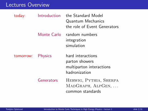
today: Introduction the Standard ModelQuantum Mechanicsthe role of Event Generators

Monte Carlo random numbersintegrationsimulation

tomorrow: Physics hard interactionsparton showersmultiparton interactionshadronization

Generators Herwig, Pythia, SherpaMadGraph, AlpGen, . . .common standards

Torbjorn Sjostrand Introduction to Monte Carlo Techniques in High Energy Physics – lecture 1 slide 2/31

The Standard Model

Matter particles:

type (shorthand) generation charge1 2 3

up-type quarks (q) u c t +2/3down-type quarks (q) d s b −1/3neutrinos (ν) νe νµ ντ 0charged leptons (`−) e µ τ −1

each with its antiparticle (q, ν, `+)

Interactions:

interaction mediatorstrong g (gluon)electromagnetic γ (photon)weak W+, W−, Z0

mass generation H (Higgs)

Hadrons:mesons qq bound by strong interactionsbaryons qqq (confinement; gluon self-interactions)

Partons: quarks and gluons bound in a hadronTorbjorn Sjostrand Introduction to Monte Carlo Techniques in High Energy Physics – lecture 1 slide 3/31

Feynman Diagrams

incomingquarks

outgoingquarks

exchangedgluon

propagator

vertex

vertex

time

space

Introduce kinematics-dependent factors for incoming, outgoingand exchanged particles, and couplings for vertices:together they give the amplitude for the process.


Quantum Mechanics

A given initial and final state typically can be relatedvia several separate intermediate histories, e.g.

qg! qg

(t) (s) (u)

Cross section σ ∝ |At + As + Au|2 6= |At |2 + |As |2 + |Au|2.

Interference ⇒ not possible to know which path process took.

If one amplitude dominates then approximate simplifications(e.g. At dominates for scattering angle → 0).

Trick : σt ∝ |At + As + Au|2|At |2

|At |2 + |As |2 + |Au|2


Fluctuations

n0 20 40 60 80 100 120 140 160 180

nP

-610

-510

-410

-310

-210

-110

1

10

210

310 CMS DataPYTHIA D6TPYTHIA 8PHOJET

)47 TeV (x10

)22.36 TeV (x10

0.9 TeV (x1)

| < 2.4η| > 0

Tp

(a)CMS NSD

Wide distribution ofthe number ofcharged particlesin an event,each particlewith continuum ofpossible momenta.

Combination ofQM processesat play.

So an infinityof final states,with a probabilisticspread of properties.


Complexity

Impossible to predict complete distribution of events from theory:

Strong interactions not solved (e.g. bound hadron states).

Even if, then production of ∼ 100 particlescomputationally impossible to handle.

Some simple tasks still ∼ solvable, e.g. qq → Z0 → `+`−.

But a quark/gluonshows up as a jet= a spray of hadrons.

Ill-defined borders+ underlying activity⇒ difficult interpretation.


Search for New Physics: an Example

SM process e.g. gg → tt → bW+bW− → b`+νbqq= lepton + missing p⊥ + 4 jets

Need to understand background to look for signal.


Event Generator Philosophy

Divide et impera (Divide and conquer/rule; Latin proverb)

Way forward:

Accept approximate framework.

Evolution in “time”: one step at a time.

Each step “simple”, e.g. n-particle → (n + 1)-particle.

Diffferent mechanisms at different “time” epochs.

Computer algorithms for physics and bookkeeping.

Generate samples of events, just like experimentalists do.

Strive to predict/reproduce average behaviour & fluctuations.

Random numbers represent quantum mechanical choices.


Welcome to Monte Carlo!


Event Generators

Three general-purpose generators:

Herwig

Pythia

Sherpa

Many others good/betterat some specific tasks.

Generators to be combined with detector simulation (Geant)accelerator/collisions ⇔ event generatordetector/electronics ⇔ detector simulation

to be used to • predict event rates and topologies• simulate possible backgrounds• study detector requirements• study detector imperfections


The Main Physics Components (in Pythia)

More tomorrow!


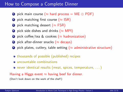
How to Compose a Complete Dinner

1 pick main course (≈ hard process = ME ⊕ PDF)

2 pick matching first course (≈ ISR)

3 pick matching dessert (≈ FSR)

4 pick side dishes and drinks (≈ MPI)

5 pick coffee/tea & cookies (≈ hadronization)

6 pick after-dinner snacks (≈ decays)

7 pick plates, cutlery, table setting (≈ administrative structure)

thousands of possible (published) recipes

uncountable combinations

never identical results (meat, spices, temperature, . . . )

Having a Higgs event ≈ having beef for dinner.(Don’t look down on the work of the chef!)


Monte Carlo Methods


Random Numbers

Truly random R :• uniform distribution 0 < R < 1• no correlations in sequence

Example: radioactive decayEvent generation + detector simulation voracious users⇒ need pseudorandom computer algorithms

Deterministic:in simplest form Ri = f (Ri−1)more sophisticated Ri = f (Ri−1,Ri−2, . . . ,Ri−k)

Examples:

name k periodoldtimers 1 ∼ 109

L’Ecuyer 3 ∼ 1026

Marsaglia-Zaman 97 ∼ 10171

Mersenne twister 623 ∼ 10600


The Marsaglia Effect

2D-array: white if R < 0.5, black if R > 0.5:

Marsaglia: recursion ⇒ multiplets (Rmi ,Rmi+1, . . . ,Rmi+m−1),i = 1, 2, . . ., fall on parallel planes in m-dimensional hypercube.A small m spells disaster. Don’t play on your own!


Spatial vs. Temporal Problems

“Spatial” problems: no memory

1 What is the land area of your home country?

2 What is the integrated cross section of a process?

“Temporal” problems: has memory

1 Traffic flow: What is probability for a car to pass a givenpoint at time t, given traffic flow at earlier times?(Lumping from red lights, antilumping from finite size of cars!)

2 Radioactive decay: what is the probability for a radioactivenucleus to decay at time t, gven that it was created at time 0?

In reality normally combined into multidimensional problems

1 What is traffic flow in a whole city?

2 What is the probability for a radioactive nucleusto decay sequentially at several different times,each time into one of several possible channels?


Spatial methods

In practical applications often need not only value of integral,but also sample of randomly distributed points inside “area”:

represents quantum mechanical spread, like real data;

allows separation of messy multidimensional problems.

pq pq

!!/Z0

M2!!/Z0 = (pq + pq)

2

p"q p"

q

p"

f

p"

f

"

Example: qq → γ∗/Z 0 → ff is 2 → 2 but can be split into steps,that consecutively provide more information on the event:

1 production qq → γ∗/Z 0, notably choice of mass Mγ∗/Z0 ;2 choice of final flavour f = d,u, s, c,b, t, e−, νe, µ

−, νµ, τ−, ντ ;3 decay γ∗/Z 0 → ff, notably choice of rest frame polar angle θ;4 further steps, up to and including detector cuts.


Simple Integration

(flat Earthapproximation)

1 Pick x coordinate at random between horizontal limits.

2 Pick y coordinate at random between vertical limits.

3 Find whether point is inside Swiss border.

4 Repeat many times and keep statistics.

Area = width× height× #inside#tries


Integration of a function

Assume function f (x),x = (x1, x2, . . . , xn), n ≥ 1,where xi ,min < xi < xi ,max,and 0 ≤ f (x) ≤ fmax.

Then

Theorem

An n-dimensional integration ≡ an n + 1-dimensional volume∫f (x1, . . . , xn) dx1 . . .dxn ≡

∫ ∫ f (x1,...,xn)

01 dx1 . . .dxn dxn+1

So Monte Carlo integration of a functionis a simple generalization of area calculation.


Hit-and-miss Monte Carlo

If f (x) ≤ fmax in xmin < x < xmax

use interpretation as an area1 select

x = xmin + R (xmax − xmin)

2 select y = R fmax (new R!)

3 while y > f (x) cycle to 1

Integral as by-product:

I =

∫ xmax

xmin

f (x) dx = fmax (xmax − xmin)Nacc

Ntry= Atot

Nacc

Ntry

Binomial distribution with p = Nacc/Ntry and q = Nfail/Ntry,so error

δI

I=

Atot

√p q/Ntry

Atot p=

√q

p Ntry=

√q

Nacc−→ 1√

Naccfor p � 1


Analytical Solution

Same probability per unit area⇒ area to right of selected xis uniformly distributed fractionof whole area:∫ x

xmin

f (x ′) dx ′ = R

∫ xmax

xmin

f (x ′) dx ′

If know primitive function F (x) and know inverse F−1(y) then

F (x)− F (xmin) = R (F (xmax)− F (xmin)) = R Atot

=⇒ x = F−1(F (xmin) + R Atot)

Example:f (x) = 2x , 0 < x < 1, =⇒ F (x) = x2

F (x)− F (0) = R (F (1)− F (0)) =⇒ x2 = R =⇒ x =√

R


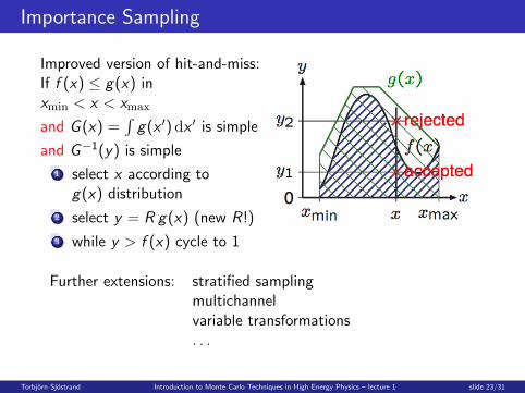
Importance Sampling

Improved version of hit-and-miss:If f (x) ≤ g(x) inxmin < x < xmax

and G (x) =∫

g(x ′) dx ′ is simple

and G−1(y) is simple

1 select x according tog(x) distribution

2 select y = R g(x) (new R!)

3 while y > f (x) cycle to 1

Further extensions: stratified samplingmultichannelvariable transformations. . .


Multidimensional Integrals

In practice almost always multidimensional integrals∫V

f (x) dx =

(∫V

g(x) dx

)× Nacc

Ntry

gives error ∝ 1/√

N irrespective of dimensionbut constant of proportionality related to amount of fluctuations.

Contrast with normal integration methods:trapezium rule error ∝ 1/N2 → 1/N2/d in d dimensions,Simpson’s rule error ∝ 1/N4 → 1/N4/d in d dimensionsso Monte Carlo methods always win in large dimensions


Temporal Methods: Radioactive Decays – 1

Consider “radioactive decay”:N(t) = number of remaining nuclei at time tbut normalized to N(0) = N0 = 1 instead, so equivalentlyN(t) = probability that (single) nucleus has not decayed by time tP(t) = −dN(t)/dt = probability for it to decay at time t

Naively P(t) = c =⇒ N(t) = 1− ct.Wrong! Conservation of probabilitydriven by depletion:a given nucleus can only decay once

CorrectlyP(t) = cN(t) =⇒ N(t) = exp(−ct)i.e. exponential dampeningP(t) = c exp(−ct)


Radioactive Decays – 2

For radioactive decays P(t) = cN(t), with c constant,but now generalize to time-dependence:

P(t) = −dN(t)

dt= f (t) N(t) ; f (t) ≥ 0

Standard solution:

dN(t)

dt= −f (t)N(t) ⇐⇒ dN

N= d(lnN) = −f (t) dt

lnN(t)−lnN(0) = −∫ t

0f (t ′) dt ′ =⇒ N(t) = exp

(−

∫ t

0f (t ′) dt ′

)F (t) =

∫ t

f (t ′) dt ′ =⇒ N(t) = exp (−(F (t)− F (0)))

N(t) = R =⇒ t = F−1(F (0)− lnR)


The Veto Algorithm

What now if f (t) has no simple F (t) or F−1,but f (t) ≤ g(t), with g “nice”?

The veto algorithm

1 start with i = 0 and t0 = 0

2 + + i (i.e. increase i by one)

3 ti = G−1(G (ti−1)− lnR), i.e ti > ti−1

4 y = R g(t)

5 while y > f (t) cycle to 2

That is, when you fail, you keep on going from the time when youfailed, and do not restart at time t = 0. (Memory!)


The Veto Algorithm: Proof

define Sg (ta, tb) = exp(−

∫ tbta

g(t ′) dt ′)

P0(t) = P(t = t1) = g(t) Sg (0, t)f (t)

g(t)= f (t) Sg (0, t)

P1(t) = P(t = t2) =

∫ t

0dt1 g(t1)Sg (0, t1)

(1− f (t1)

g(t1)

)g(t) Sg (t1, t)

f (t)

g(t)

= f (t) Sg (0, t)

∫ t

0dt1 (g(t1)− f (t1)) = P0(t) Ig−f

P2(t) = · · · = P0(t)

∫ t

0dt1 (g(t1)− f (t1))

∫ t

t1

dt2 (g(t2)− f (t2))

= P0(t)

∫ t

0dt1 (g(t1)− f (t1))

∫ t

0dt2 (g(t2)− f (t2)) θ(t2 − t1)

= P0(t)1

2

(∫ t

0dt1 (g(t1)− f (t1))

)2

= P0(t)1

2I 2g−f

P(t) =∞∑i=0

Pi (t) = P0(t)∞∑i=0

I ig−f

i != P0(t) exp(Ig−f )

= f (t) exp

(−

∫ t

0g(t ′) dt ′

)exp

(∫ t

0dt1 (g(t1)− f (t1))

)= f (t) exp

(−

∫ t

0f (t ′) dt ′

)Torbjorn Sjostrand Introduction to Monte Carlo Techniques in High Energy Physics – lecture 1 slide 28/31

The winner takes it all

Assume “radioactive decay” with two possible decay channels 1&2

P(t) = −dN(t)

dt= f1(t)N(t) + f2(t)N(t)

Alternative 1:use normal veto algorithm with f (t) = f1(t) + f2(t).Once t selected, pick decays 1 or 2 in proportions f1(t) : f2(t).

Alternative 2:

The winner takes it all

select t1 according to P1(t1) = f1(t1)N1(t1)and t2 according to P2(t2) = f2(t2)N2(t2),i.e. as if the other channel did not exist.If t1 < t2 then pick decay 1, while if t2 < t1 pick decay 2.


The winner takes it all: proof

P1(t) = (f1(t) + f2(t)) exp

(−

∫ t

0(f1(t

′) + f2(t′))dt ′

)f1(t)

f1(t) + f2(t)

= f1(t) exp

(−

∫ t

0(f1(t

′) + f2(t′))dt ′

)= f1(t) exp

(−

∫ t

0f1(t

′) dt ′)

exp

(−

∫ t

0f2(t

′) dt ′)

Algorithm especially convenient when temporal and/or spatialdependence of f1 and f2 are rather different.


Summary

Nature is Quantum Mechanical.

LHC events contain infinite variability.

Use random numbers to pick among possible outcomes,

to give complete computer-generated LHC events,

hopefully predicting/reproducing average and spreadof any observable quantity.

Tomorrow:

A closer look at some of the key physics componentsof generators.

A survey of existing generators.


introduction to monte carlo techniques in high energy...

Documents