LADAR Image Visualization Tool

By: Robin R. Burton

A S in g le P u lse . . .

L ase r

A tm o sp h e ricA tten u a tio n(U p /D o w n )

A e ro so lS ca tte r

T o p o g ra p h ica lS ca tte r

B e amS p re ad

S h o rt-te rmb ro a d e n in g

L o n g -te rmb ro a d e n in g

C e n tro idW an d e r

(P u lse to p u lse )

M u ltip leB o u n ce

O v erla p(G F F )

Temporal Pulse

0

0.2

0.4

0.6

0.8

1

1.2

4 3.5 3 2.5 2 1.5 1 0.5 0

Se conds

Pow

er

T em p o ra l S h ap e

Pow

er

S eco n d s

Temporal Pulse

0

0.2

0.4

0.6

0.8

1

1.2

4 3.5 3 2.5 2 1.5 1 0.5 0

S e conds

Po

wer

S p e c tra l S h ap e

Pow

er

W av e len g th

x

yS p a tia l S h a p e

S p e ck le P a tte rn

•S c in tilla tio n•P a th D o w n• P a th U p

• R e flec tio n fr o m g ro u n d

F o c a l P lan e

Im ag e D a n c in g(P u lse to p u lse )

F o c a l P lan e

Im ag e B lu r(M T F )

• G au ss ian • U serD efin ed

• G au ss ian• T o p H atP assiv e

(A c tiv e )

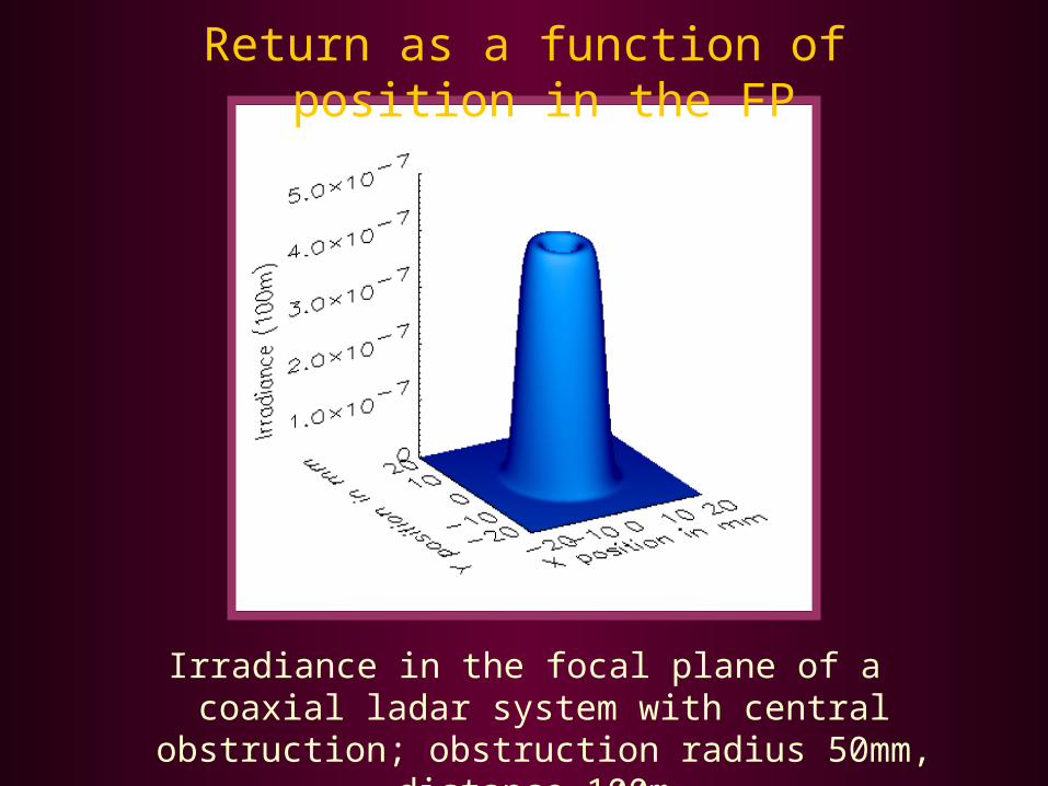
Irradiance in the focal plane of a coaxial ladar system with central obstruction; obstruction radius 50mm, distance

100m

Return as a function of position in the FP

Simulated return for a single pixel as a function of range (hard target return)

1.00E-12

1.00E-11

1.00E-10

1.00E-09

1.00E-08

1.00E-07

1.00E-06

0.00E+00 1.00E+07 2.00E+07 3.00E+07 4.00E+07 5.00E+07 6.00E+07

mm

Wa

tts

config1-trial3

config1-trial2

config1-trial1

1.00E-09

1.00E-08

1.00E-07

1.00E-06

0.00E+00 1.00E+06 2.00E+06 3.00E+06 4.00E+06 5.00E+06 6.00E+06 7.00E+06 8.00E+06 9.00E+06 1.00E+07

Noncoaxial lidar system, system separation 1m, inclination angle as indicated, other parameters as in Table I.

1.00E-10

1.00E-09

1.00E-08

1.00E-07

1.00E-06

1.00E+05 1.00E+06 1.00E+07

Range (mm)

Po

wer

(W)

0 mrad

.2 mrad

.5 mrad

1 mrad

2 mrad

5 mrad

Simulated return for a single pixel as a function of range (aerosol return)

Function of Wavelength

1.00E-15

1.00E-14

1.00E-13

1.00E-12

1.00E-11

1.00E-10

1.00E+05 1.01E+07 2.01E+07 3.01E+07 4.01E+07 5.01E+07 6.01E+07

Det 0, Wavelength 0

Det 0, Wavelength 1

Det 0, Band

Data Structure

R1

R2

R3

R4

R5

R6

y1

x1

1

R1

R2

R3

R4

R5

R6

y1

x1

2

1.00E-10

1.00E-09

1.00E-08

1.00E-07

1.00E-06

1.00E-05

1.00E+07 1.50E+07 2.00E+07 2.50E+07 3.00E+07 3.50E+07 4.00E+07 4.50E+07 5.00E+07 5.50E+07

Range (mm)

Po

wer

(W)

Down a pixel(Range)

Absorption Feature

0.01

0.1

1

10

100

4 5 6 7 8 9 10 11 12

Wavenumber

Po

we

r

Peak of Absorption Feature

Wing of Absorption Feature1 2 Across cubes

(Spectra)

DAS / Differential Absorption LADAR (DIAL)

• Technique– Ratio of the peak of an absorption feature to the wing of the same

feature

• Many molecules have narrow features in the 5-12 m region– Used to uniquely identify specific molecules

• 3D concentration maps• Using assumptions

– Density– Pressure– temperature

– Uses tunable lasers

Absorption Feature

0.01

0.1

1

10

100

4 5 6 7 8 9 10 11 12

Wavenumber

Po

we

rPeak of Absorption Feature

Wing of Absorption Feature

1 2

Topographic• Scatter off a solid target

– Laser rangefinder– Can create digital terrain

elevation maps

Normalized

1.00E-10

1.00E-09

1.00E-08

1.00E-07

1.00E-06

1.00E-05

1.00E+07 1.50E+07 2.00E+07 2.50E+07 3.00E+07 3.50E+07 4.00E+07 4.50E+07 5.00E+07 5.50E+07

Range (mm)

Po

wer

(W)