Multi-Agent SystemsLecture 10 & 11Lecture 10 & 11

University “Politehnica” of Bucarest2004-2005

Adina Magda Floreaadina@cs.pub.ro

http://turing.cs.pub.ro/blia_2005

Machine LearningMachine LearningLecture outlineLecture outline

1 Learning in AI (machine learning)1 Learning in AI (machine learning)2 Learning decision trees2 Learning decision trees3 Version space learning3 Version space learning4 Reinforcement learning4 Reinforcement learning5 Learning in multi-agent systems5 Learning in multi-agent systems

5.1 Learning action coordination5.1 Learning action coordination5.2 Learning individual performance5.2 Learning individual performance5.3 Learning to communicate5.3 Learning to communicate5.4 Layered learning5.4 Layered learning

6 Conclusions6 Conclusions

3

1 Learning in AI1 Learning in AI What is machine learning?

Herbet Simon defines learning as:“any change in a system that allows it to

perform better the second time on repetition of the same task or another task drawn from the same population (Simon, 1983).”

In ML the agent learns: knowledge representation of the problem domain problem solving rules, inferences problem solving strategies

4

Classifying learning

In MAS learning the agents should learn: what an agent learns in ML but in the context of MAS -

both cooperative and self-interested agents how to cooperate for problem solving - cooperative agents how to communicate - both cooperative and self-

interested agents how to negotiate - self interested agents

Different dimensions explicitly represented domain knowledge how the critic component (performance evaluation) of a

learning agent works the use of knowledge of the domain/environment

5

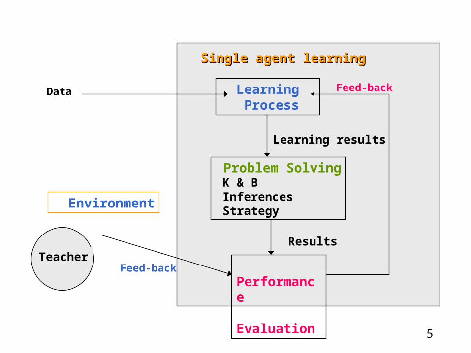
Single agent learningSingle agent learning

Learning Process

Problem Solving K & B Inferences Strategy

Performance Evaluation

Learning results

Results

Environment

Feed-backTeacher

Feed-backData

6

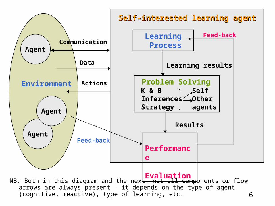
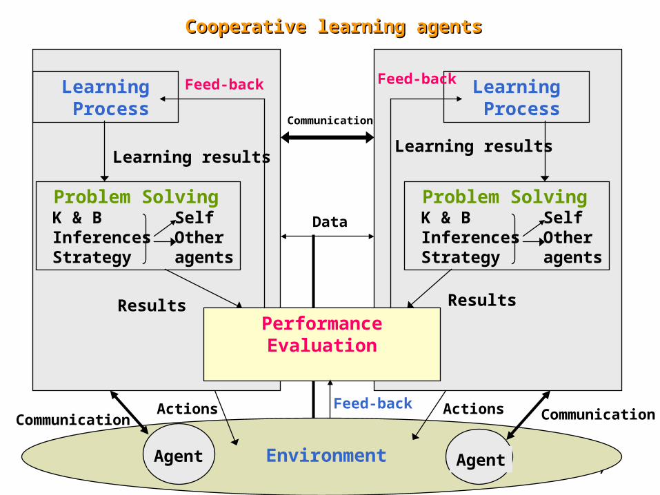
NB: Both in this diagram and the next, not all components or flow arrows are always present - it depends on the type of agent (cognitive, reactive), type of learning, etc.

Self-interested learning agentSelf-interested learning agent

Learning Process

Problem Solving K & B Self Inferences Other Strategy agents

Performance Evaluation

Learning results

Results

Environment

Communication

Actions

Feed-backAgent

Agent

Agent

Feed-back

Data

7

Learning Process

Problem Solving K & B Self Inferences Other Strategy agents

Learning results

Results Results

Learning Process

Problem Solving K & B Self Inferences Other Strategy agents

Learning results

Cooperative learning agentsCooperative learning agents

PerformanceEvaluation

EnvironmentAgent Agent

Communication CommunicationActions ActionsFeed-back

Feed-backFeed-back

Data

Communication

8

2 Learning decision trees ID3 - Quinlan -’80 ID3 algorithm classifies training examples in several classes Training examples: attributes and values2 phases: build decision tree use tree to classify unknown instances

Decision tree - definition2 3 1

Shape Color Size Classificationcircle red small +circle red big +triangle yellow small -circle yellow small -triangle red big -circle yellow big -

9

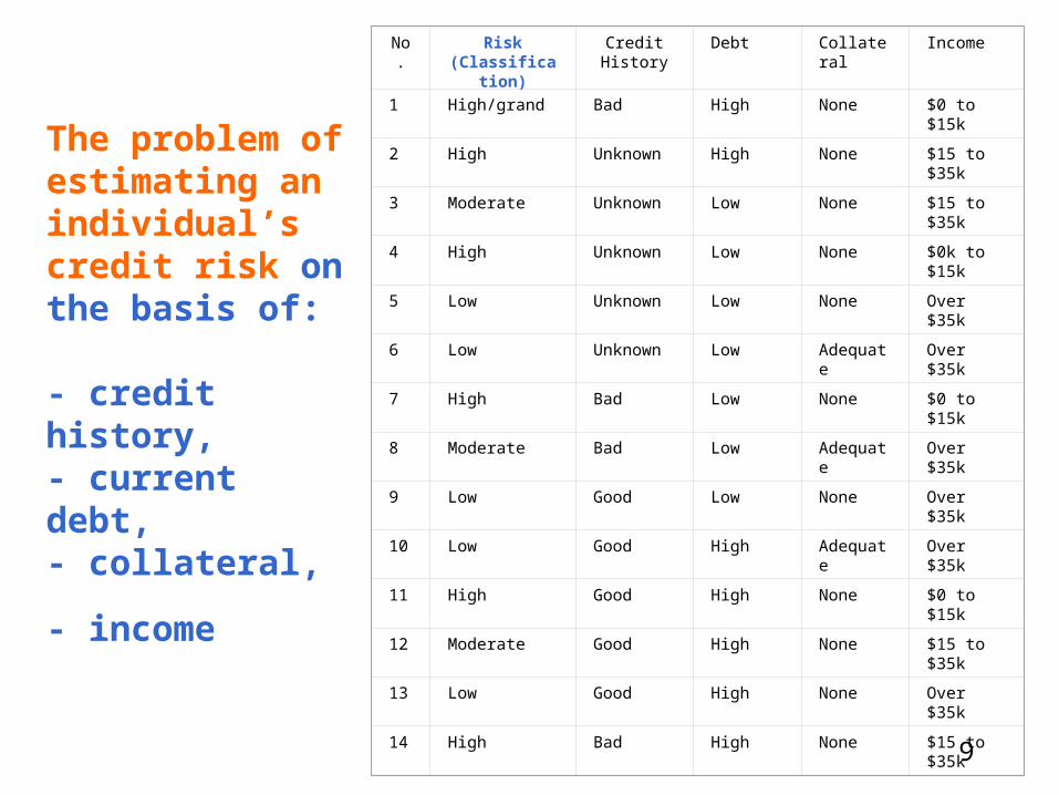
The problem of estimating an individual’s credit risk on the basis of:

- credit history,- current debt,- collateral,

- income

No.

Risk (Classification)

Credit History

Debt Collateral Income

1 High/grand Bad High None $0 to $15k

2 High Unknown High None $15 to $35k

3 Moderate Unknown Low None $15 to $35k

4 High Unknown Low None $0k to $15k

5 Low Unknown Low None Over $35k

6 Low Unknown Low Adequate Over $35k

7 High Bad Low None $0 to $15k

8 Moderate Bad Low Adequate Over $35k

9 Low Good Low None Over $35k

10 Low Good High Adequate Over $35k

11 High Good High None $0 to $15k

12 Moderate Good High None $15 to $35k

13 Low Good High None Over $35k

14 High Bad High None $15 to $35k

Income?

High risk Credit history?

Low risk Moderate riskDebt?

Credit history?

High riskHigh risk Moderate risk

Moderate riskHigh risk

$0K-$15K

$15K-$35K

$Over 35K

Unknown Bad Good

High Low

UnknownBad

Good

Decision tree

ID3 assumes the simplest decision tree that covers all the training examples is the one it should be picked.Ockham’s Razor (or Occam ??), 1324:“It is vain to do with more what can be done with less…

Entities should not be multiplied beyond necessity.”

Information theoretic test selection in ID3 Information theory – the info content of a message M={m1, …, mn}, p(mi) The information content of the message M

I(M) = Sumi=1,n[-p(mi)*log2(p(mi))]

I(Coin_toss) = - p(heads)log2(p(heads)) – p(tails)log2(p(tails) = -1/2log2(1/2) – 1/2log2(1/2) = 1 bit

I(Coin_toss) = - p(heads)log2(p(heads)) – p(tails)log2(p(tails) = -3/4log2(3/4) – 1/4log2(1/4) = 0.811 bits

p(risk_high) = 6/14

p(risk_moderate) = 3/14

p(risk_low) = 5/14

The information in any tree that covers the examples

I(Tree) = -6/14log2(6/14)-3/14log2(3/14)-5/14log2(5/14)

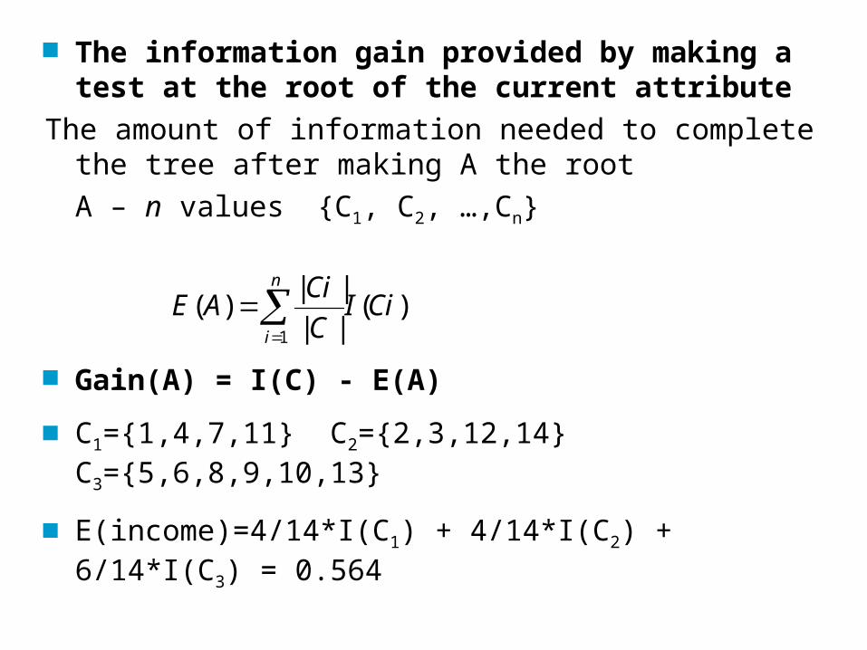
The information gain provided by making a test at the root of the current attribute

The amount of information needed to complete the tree after making A the root

A – n values {C1, C2, …,Cn}

Gain(A) = I(C) - E(A)

C1={1,4,7,11} C2={2,3,12,14} C3={5,6,8,9,10,13}

E(income)=4/14*I(C1) + 4/14*I(C2) + 6/14*I(C3) = 0.564

)(||

||)(

1

CiIC

CiAE

n

i

Assesing the performance of ID3Training set and test set – average prediction of quality,

happy graphs Broadening the applicability of decision trees Missing data: how to classify an instance that is missing

one of test attributes?Pretend the instance has all possible values for the attribute, weight each value according to its frequency among the examples, follow all branches and multiply weights along the path

Multivalued attributes: an attribute with a large number of possible values – gain ratiogain ratio = selects attributes according to

Gain(A)/I(CA) Continuous-valued attributes - discretize

14

3 Version space learning P and Q – sets that match p, q in FOPL

Expression p is more general than q iff P Q - we say that p covers q

color(X,red) color(ball,red)

If a concept p is more general than a concept q then p(x), q(x) descriptions that classify objects as being positive examples:

x p(x) positive(x) x q(x) positive(x)

p covers q iff q(x) positive(x) is a logical consequence of p(x) positive(x)

Concept spaceobj(X,Y,Z)

A concept c is maximally specific if it covers all positive examples, none of the negative examples, and for any other concept c’ that covers the positive examples, c’ is more general than c - S

A concept c is maximally general if it covers none of the negative examples, and for any other concept c’ that covers none negative examples, c is more general than c’ - G

15

The candidate elimination algorithm Algorithms for searching the concept space; overgeneralization,

overspecialization

Specific to general search for hypothesis set S:maximally specific

generalizations Initialize S to the first positive training instance Be N the set of all negative instances seen so far for each positive instance p do

– for every sS do if s does not match p, replace s with its most specific generalization that matches p

– delete from S all hypotheses more general than some other hypothesis in S

– delete from S all hypotheses that match a previously observed negative instance in N

for every negative instance n do– delete all members of S that match n– add n to N to check future hypotheses for overgeneralization

16

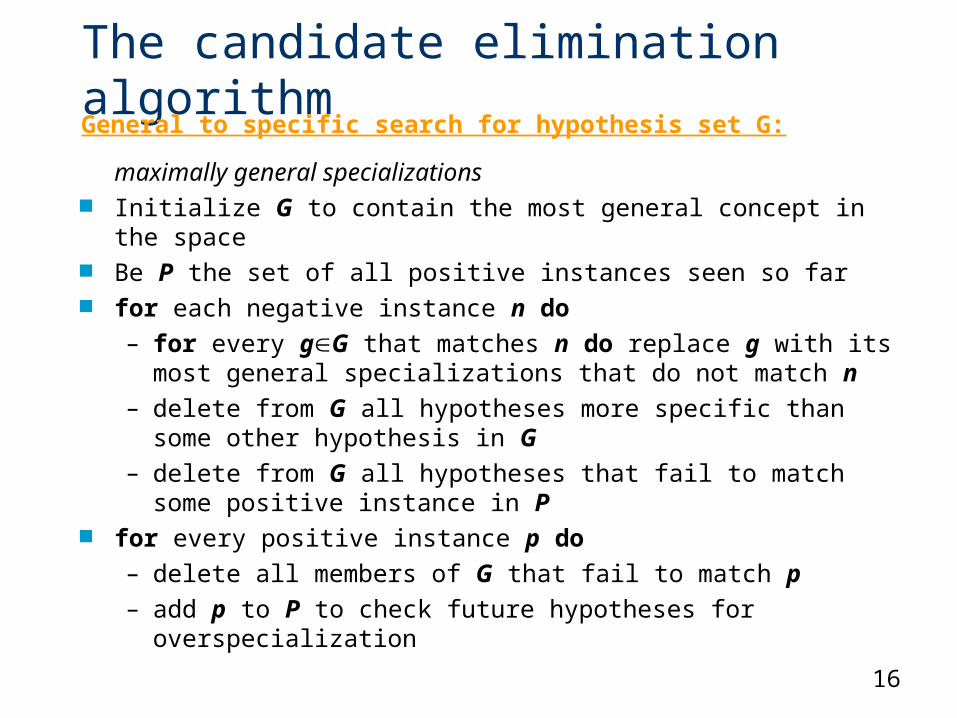
The candidate elimination algorithmGeneral to specific search for hypothesis set G:

maximally general specializations Initialize G to contain the most general concept in the space Be P the set of all positive instances seen so far for each negative instance n do

– for every gG that matches n do replace g with its most general specializations that do not match n

– delete from G all hypotheses more specific than some other hypothesis in G

– delete from G all hypotheses that fail to match some positive instance in P

for every positive instance p do– delete all members of G that fail to match p– add p to P to check future hypotheses for overspecialization

17

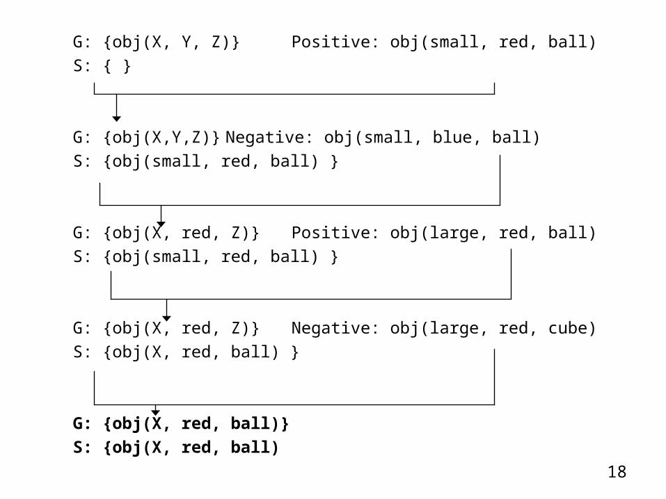
Bidirectional search; S and G

Candidate elimination Initialize S to the first positive training instance for each positive instance p do

– delete from G all hypotheses that fail to match p– for every sS do if s does not match p, replace s with its most

specific generalization that matches p– delete from S all hypotheses more general than some other

hypothesis in S– delete from S all hypotheses more general than some hypothesis

in G for every negative instance n do

– delete all members of S that match n– for every gG that matches n do replace g with its most general

specializations that do not match n– delete from G all hypotheses more specific than some other

hypothesis in G– delete from G all hypotheses more specific than some other

hypothesis in S

18

G: {obj(X, Y, Z)} Positive: obj(small, red, ball)

S: { }

G: {obj(X,Y,Z)} Negative: obj(small, blue, ball)

S: {obj(small, red, ball) }

G: {obj(X, red, Z)} Positive: obj(large, red, ball)

S: {obj(small, red, ball) }

G: {obj(X, red, Z)} Negative: obj(large, red, cube)

S: {obj(X, red, ball) }

G: {obj(X, red, ball)}

S: {obj(X, red, ball)

19

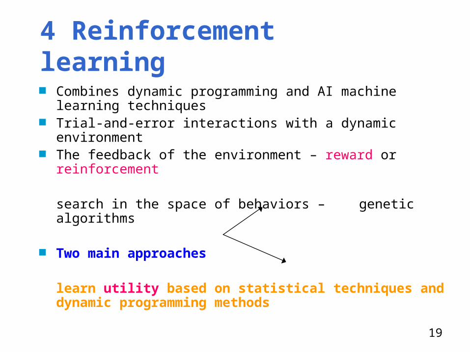
4 Reinforcement learning

Combines dynamic programming and AI machine learning techniques

Trial-and-error interactions with a dynamic environment The feedback of the environment – reward or reinforcement

search in the space of behaviors – genetic algorithms

  Two main approaches 

learn utility based on statistical techniques and dynamic programming methods

20

A reinforcement-learning model

B – agent's behaviori – input = current state of the envr – value of reinforcement (reinforcement signal)T – model of the world

The model consists of:-         a discrete set of environment states S (sS)-         a discrete set of agent actions A (a A)-         a set of scalar reinforcement signals, typically {0, 1} or real numbers- the transition model of the world, T

• environment is nondeterministicT : S x A P(S) – T = transition model T(s, a, s’)

Environment history = a sequence of states that leads to a terminal state

i

T

I

R B

E

s

a

r

21

Features varying RL accessible / inaccessible environment has (T known) / has not a model of the environment learn behavior / learn behavior + model reward received only in terminal states or in any state passive/active learner:

– learn utilities of states (state-action) – active learner – learn also what to do

how does the agent represent B, namely its behavior:– utility functions on states or state histories (T is

known)– active-value functions (T is not necessarily known) -

assigns an expected utility to taking a given action in a given state

E(a,e) =e’env(e,a)(prob(ex(a,e)=e’)*utility(e’))

22

The RL problem the agent has to find a policy = a function which

maps states to actions and which maximizes some long-time measure of reinforcement.

The agent has to learn an optimal behavior = optimal policy = a policy which yields the highest expected utility

The utility function depends on the environment history (a sequence of states)

In each state s the agents receives a reward - R(s)

Uh([s0, s1, …, sn]) – utility function on histories

23

Models of optimal behavior Finite-horizon model: at a given moment of time the agent

should optimize its expected reward for the next h steps

E(t=0, h R(st))

 rt represents the reward received t steps into the future.

  Infinite-horizon model: optimize the long-run reward

  E(t=0, R(st))

  Infinite-horizon discounted model: optimize the long-run

reward but rewards received in the future are geometrically discounted according to a discount factor .

  E(t=0, t R(st))

0 < 1.

24

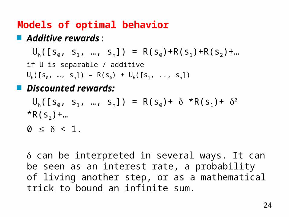
Models of optimal behavior Additive rewards:

  Uh([s0, s1, …, sn]) = R(s0)+R(s1)+R(s2)+…if U is separable / additive

Uh([s0, …, sn]) = R(s0) + Uh([s1, .., sn])

Discounted rewards:

  Uh([s0, s1, …, sn]) = R(s0)+ *R(s1)+ 2 *R(s2)+…

0 < 1.

can be interpreted in several ways. It can be seen as an interest rate, a probability of living another step, or as a mathematical trick to bound an infinite sum.

25

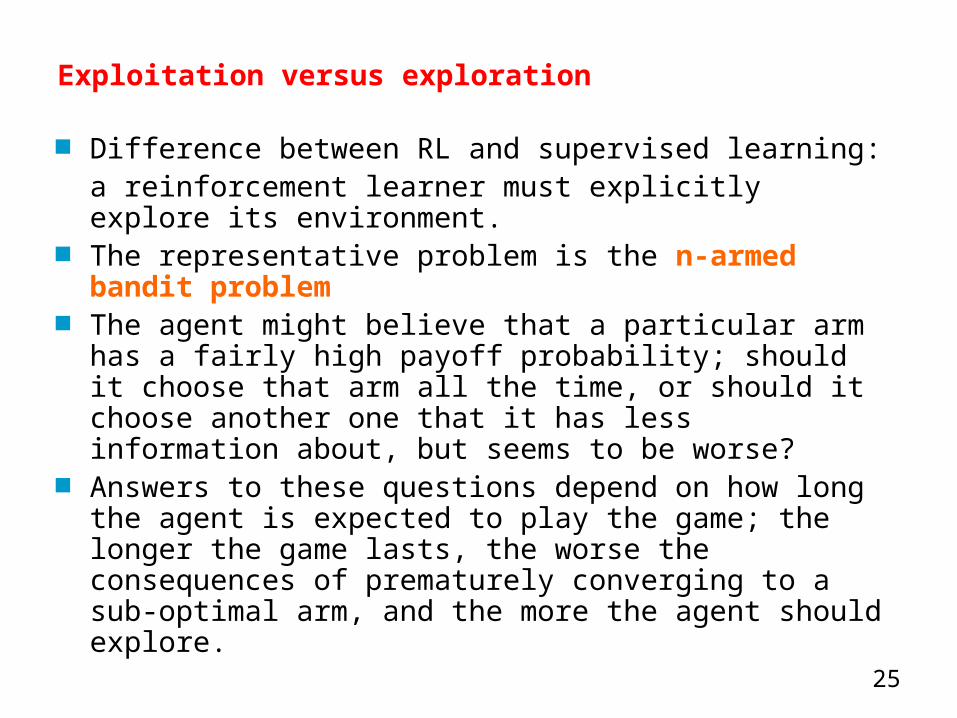
Exploitation versus exploration

Difference between RL and supervised learning:a reinforcement learner must explicitly explore its environment.

The representative problem is the n-armed bandit problem

The agent might believe that a particular arm has a fairly high payoff probability; should it choose that arm all the time, or should it choose another one that it has less information about, but seems to be worse?

Answers to these questions depend on how long the agent is expected to play the game; the longer the game lasts, the worse the consequences of prematurely converging to a sub-optimal arm, and the more the agent should explore.

26

 Utilities of states Utility of a state defined in terms of the utility of a state

sequence = expected utility of the state sequence that might follow it, if the agents follows the policy

 U (s) = E(H(s,) | T) = (P(H(s, )| T) * Uh(H(s, )))• H – history beginning in s• E- expected utility Uh – utility function on histories - is a policy defined by the transition model T and the utility

function on histories Uh. • If U is separable / additive:

Uh([s0, …, sn]) = R(s0) + Uh([s1, .., sn])

st – the state after executing t steps using  U(s) = E(t=0, (t *R(st) | , s0=s)

U(s) long term, R(s) short term

27

 A 4 x 3 environment The intended outcome occurs with probability 0.8,

and with probability 0.2 (0.1, 0.1) the agent moves at right angles to the intended direction.

The two terminal states have reward +1 and –1, all other states have a reward of –0.04, =1

+1

-1

0.1 0.1

0.8

+1

-1

0.812 0.868 0.918

0.762

0.705

0.660

0.655 0.611 0.388

1 2 3 4

3

2

1

3

2

1

1 2 3 4

28

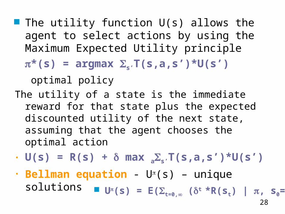
The utility function U(s) allows the agent to select actions by using the Maximum Expected Utility principle

*(s) = argmax s’T(s,a,s’)*U(s’)

 optimal policy

The utility of a state is the immediate reward for that state plus the expected discounted utility of the next state, assuming that the agent chooses the optimal action

• U(s) = R(s) + max as’T(s,a,s’)*U(s’)

• Bellman equation - U(s) – unique solutions

 U(s) = E(t=0, (t *R(st) | , s0=s)

+1

-1

0.812 0.868 0.918

0.762

0.705

0.660

0.655 0.611 0.388

3

2

1

1 2 3 4

Bellman equation for the 4x3 worldEquation for the state (1,1)U(1,1) = -0.04 + max{ 0.8 U(1,2) + 0.1 U(2,1) + 0.1 U(1,1),

Up 0.9U(1,1) + 0.1U(1,2),

Left 0.9U(1,1) + 0.1U(2,1),

Down 0.8U(2,1) +0.1U(1,2) + 0.1U(1,1)}

Right

Up is the best action

30

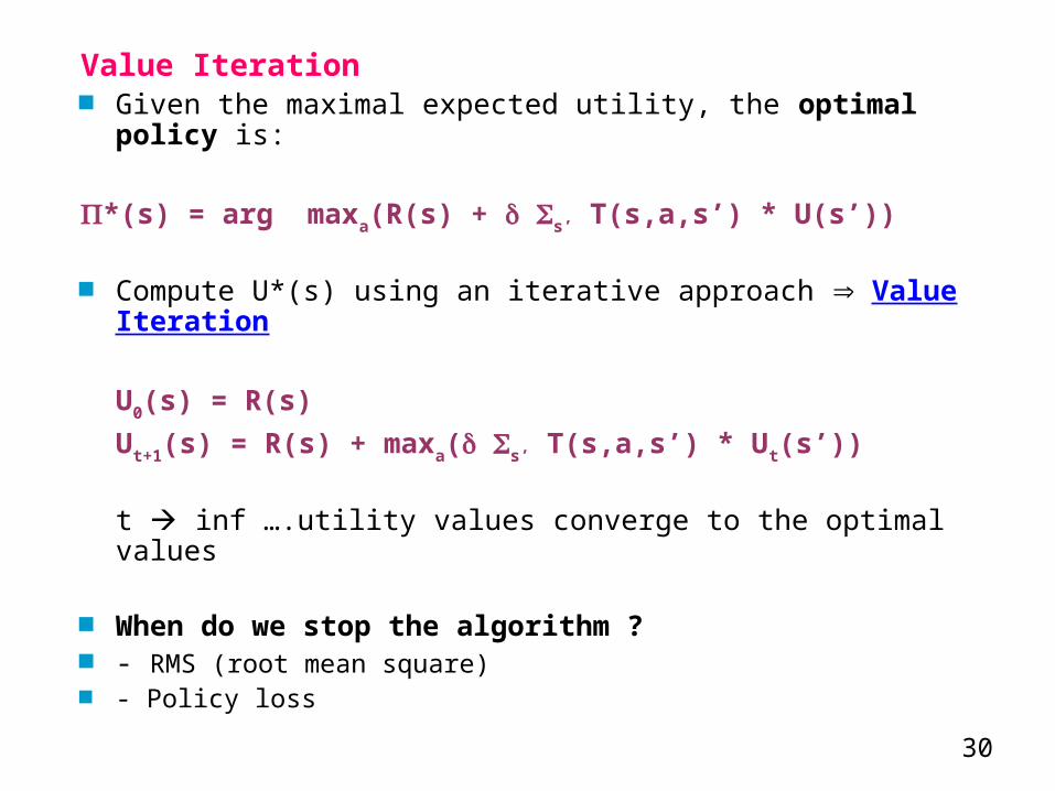
Value Iteration Given the maximal expected utility, the optimal policy is: 

*(s) = arg maxa(R(s) + s’ T(s,a,s’) * U(s’))  Compute U*(s) using an iterative approach Value Iteration 

U0(s) = R(s)

Ut+1(s) = R(s) + maxa( s’ T(s,a,s’) * Ut(s’)) 

t inf ….utility values converge to the optimal values  When do we stop the algorithm ? - RMS (root mean square) - Policy loss

31

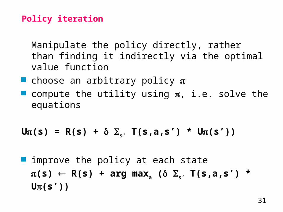
Policy iteration

Manipulate the policy directly, rather than finding it indirectly via the optimal value function

choose an arbitrary policy compute the utility using , i.e. solve the equations

U(s) = R(s) + s’ T(s,a,s’) * U(s’))

improve the policy at each state

(s) R(s) + arg maxa ( s’ T(s,a,s’) * U(s’))

32

a) Passive reinforcement learningADP (Adaptive Dynamic Programming) learning The problem of calculating an optimal policy in an accessible,

stochastic environment.

  Markov Decision Problem (MDP) consists of:

<S, A, P, R> S - a set of statesA - a set of actionsR – reward function, R: S x A RT : S x A (S), with (S) the probability distribution

over the states S The model is Markov if the state transitions are independent of any previous environment states or agent actions.

MDP: finite-state and finite-action – focus on that / infinite state and action space

Finding the optimal policy given a model T = calculate the utility of each state U(state) and use state utilities to select an optimal action in each state.

33

The utility of a state s is given by the expected utility of the history beginning at that state and following an optimal policy.

  If the utility function is separable

U(s) = R(s) + maxas’ T(s,a,s’) * U(s’), s (1)(this is a dynamic programming technique)  The equation asserts that the utility of a state s is the expected

instantaneous reward plus the expected utility (expected discounted utility) of the next state, using the best available action.

The maximal expected utility, considering moments of time t0, t1, …, is 

U*(s) = max E(t=0,inf t rt ) - the discount factor

 

This is the expected infinite discounted sum of reward that the agent will gain if it is in state s and executes an optimal policy. This optimal value is unique and can be defined as the solution of the simultaneous equations (1).

34

ADP (Adaptive Dynamic Programming) learningfunction Passive-ADP-Agent(percept) returns an actioninputs: percept, a percept indicating the current state s’ and reward signal r’variable: , a fixed policy

mdp, an MDP with model T, rewards R, discount U, a table of utilities, initially emptyNsa, a table of frequencies for state-action pairs, initially zeroNsas’, a table of frequencies of state-action-state triples, initially

zeros, a, the previous state and action, initially null

if s’ is new then U[s’] r’, R[s’] r’if s is not null then

increment Nsa[s,a] and Nsas’[s,a,s’]for each t such that Nsas’[s,a,t] <>0 do

T[s,a,t] Nsas’[s,a,t] / Nsa[s,a]U Value-Determination(,U,mdp)if Terminal[s’] then s,a null else s,a s’, [s’]return aend

35

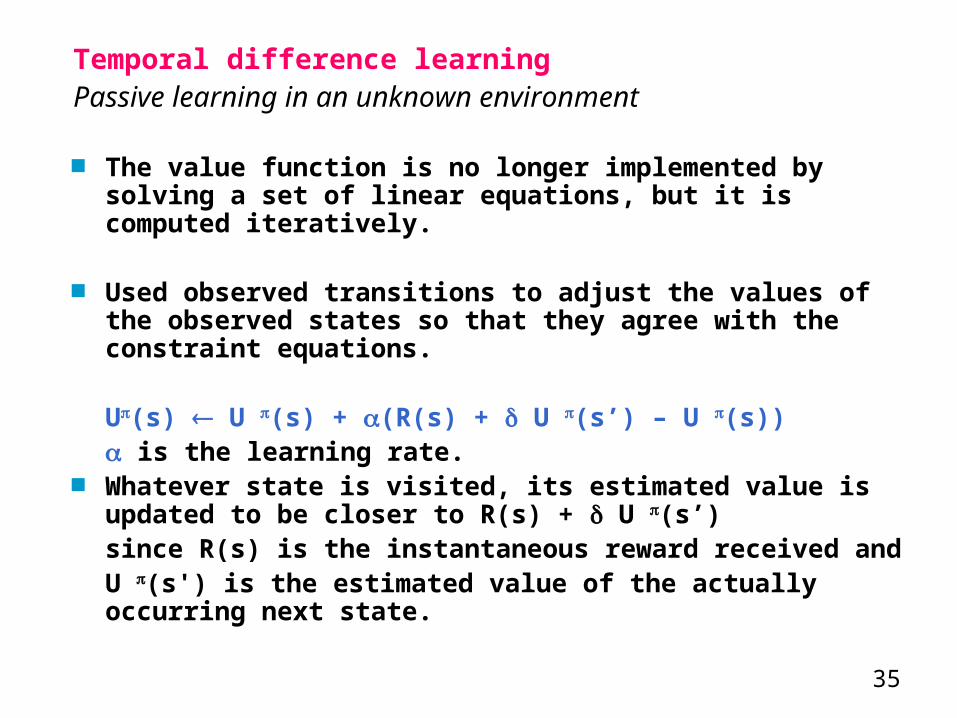
Temporal difference learningPassive learning in an unknown environment  The value function is no longer implemented by solving a

set of linear equations, but it is computed iteratively.  Used observed transitions to adjust the values of the

observed states so that they agree with the constraint equations.

 U(s) U (s) + (R(s) + U (s’) – U (s))

  is the learning rate. Whatever state is visited, its estimated value is updated

to be closer to R(s) + U (s’)since R(s) is the instantaneous reward received andU (s') is the estimated value of the actually occurring next state.

36

Temporal difference learningfunction Passive-TD-Agent(percept) returns an action

inputs: percept, a percept indicating the current state s’ and reward signal r’

variable: , a fixed policy

U, a table of utilities, initially empty

Ns, a table of frequencies for states, initially zero

s, a, r, the previous state, action, and reward, initially null

if s’ is new then U[s’] r’

if s is not null then

increment Ns[s]

U[s] U[s] + (Ns[s])(r + U [s’] – U [s])

if Terminal[s’] then s, a, r null else s, a, r s’, [s’], r’

return a

end

37

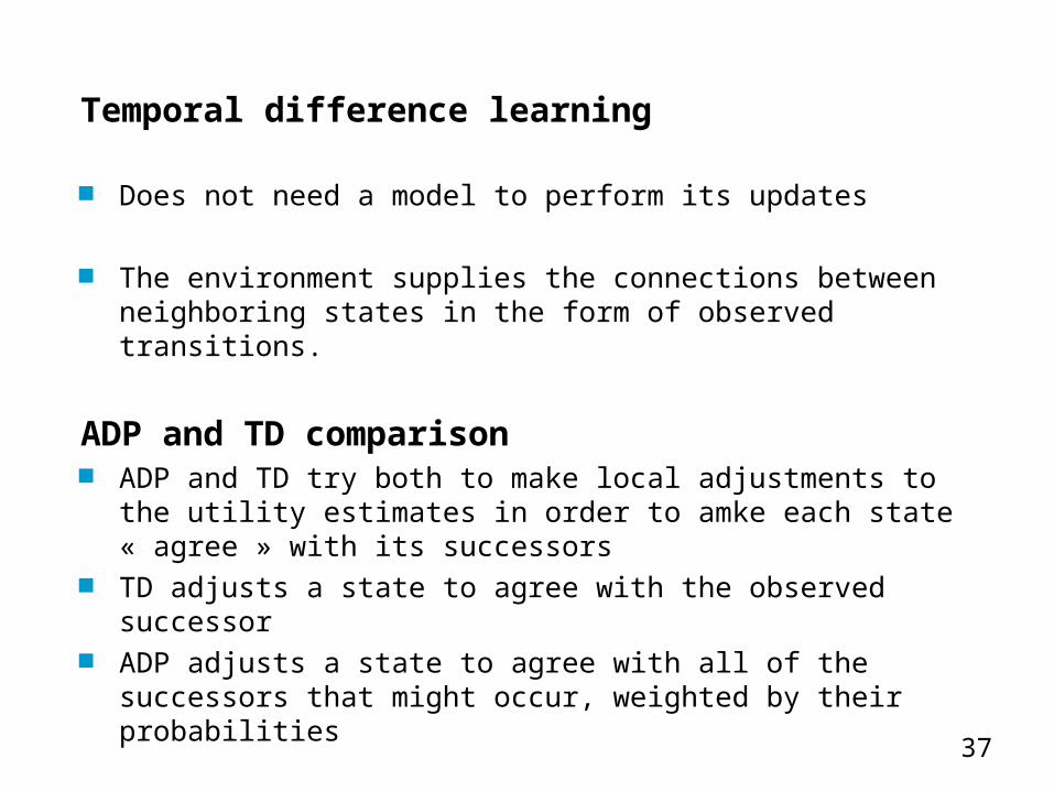
Temporal difference learning

Does not need a model to perform its updates

The environment supplies the connections between neighboring states in the form of observed transitions.

ADP and TD comparison ADP and TD try both to make local adjustments to the utility

estimates in order to amke each state « agree » with its successors TD adjusts a state to agree with the observed successor ADP adjusts a state to agree with all of the successors that might

occur, weighted by their probabilities

38

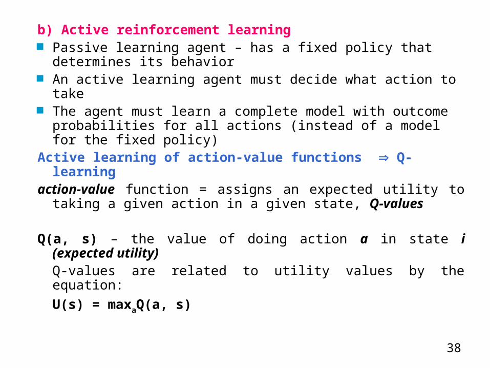
b) Active reinforcement learning Passive learning agent – has a fixed policy that

determines its behavior An active learning agent must decide what action to take The agent must learn a complete model with outcome

probabilities for all actions (instead of a model for the fixed policy)

Active learning of action-value functions Q-learningaction-value function = assigns an expected utility to taking a

given action in a given state, Q-values

Q(a, s) – the value of doing action a in state i (expected utility)Q-values are related to utility values by the equation:

U(s) = maxaQ(a, s) 

39

Active learning of action-value functions Q-learning TD learning, unknown environment 

Q(a,s) Q(a,s) + (R(s) + maxa’Q(a’, s’) – Q(a,s)) calculated after each transition from state s to s’.   Is it better to learn a model and a utility function or to learn an

action-value function with no model?

40

Q-learningfunction Q-Learning-Agent(percept) returns an action

inputs: percept, a percept indicating the current state s’ and reward signal r’

variable: Q, a table of action values index by state and action

Nsa, a table of frequencies for state-action pairs

s, a, r the previous state, action, and reward, initially null

if s is not null then

increment Nsa[s,a]

Q[a,s] Q[a,s] + (Nsa[s,a])(r + maxa’Q [a’,s’] – Q [a,s])

if Terminal[s’] then s, a, r null

else s, a, r` s’, argmaxa’ f(Q[a’, s’], Nsa[a’,s’]), r’

return a

endf(u,n) – increasing in u and decreasing in n

41

Generalization of RL  The problem of learning in large spaces is addressed

through generalization techniques, which allow compact storage of learned information and transfer of knowledge between "similar" states and actions.

  The RL algorithms include a variety of mappings, including

S A (policies), S R (value functions), S A R (Q functions and rewards), S A S (deterministic transitions), and S A S [0, 1] (transitions probabilities).

Some of these, such as transitions and immediate rewards, can be learned using straightforward supervised learning.

Popular techniques: various neural network methods, fuzzy logic, logical approaches to generalization.

42

5 Learning in MAS

The credit-assignment problem (CAP) = the problem of assigning feed-back (credit or blame) for an overall performance of the MAS Increase, decrease) to each agent that contributed to that change

inter-agent CAP = assigns credit or blame to the external actions of agents

intra-agent CAP = assigns credit or blame for a particular external action of an agent to its internal inferences and decisions

distinction not always obvious one or another

43

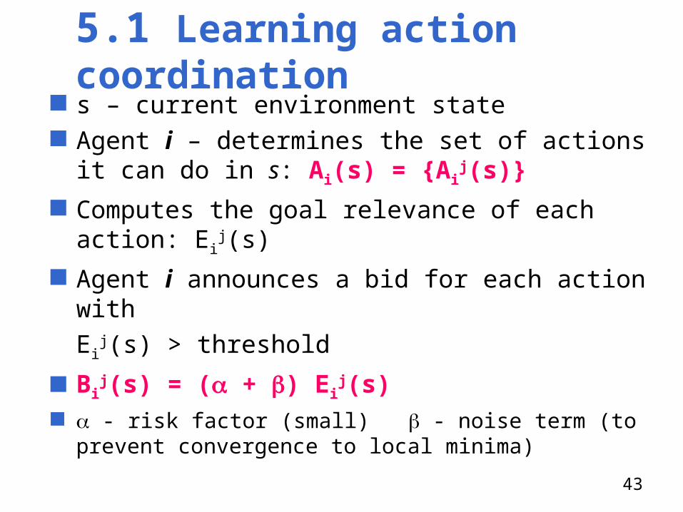
5.1 Learning action coordination s – current environment state Agent i – determines the set of actions it can do

in s: Ai(s) = {Aij(s)}

Computes the goal relevance of each action: Ei

j(s)

Agent i announces a bid for each action with

Eij(s) > threshold

Bij(s) = ( + ) Ei

j(s) - risk factor (small) - noise term (to prevent

convergence to local minima)

44

The action with the highest bid is selected Incompatible actions are eliminated Repeat process until all actions in bids are either selected

or eliminated A – selected actions = activity context

Execute selected actions Update goal relevance for actions in A

Eij(s) Ei

j(s) – Bij(s) + (R / |A|)

R –external reward received Update goal relevance for actions in the previous activity

context Ap (actions Akl)

Ekl(sp) Ek

l(sp) + (AijA Bij(s)/ |Ap|)

45

5.2 Learning individual performance

The agent learns how to improve its individual performance in a multi-agent settings

Examples Cooperative agents - learning

organizational roles Competitive agents - learning from

market conditions

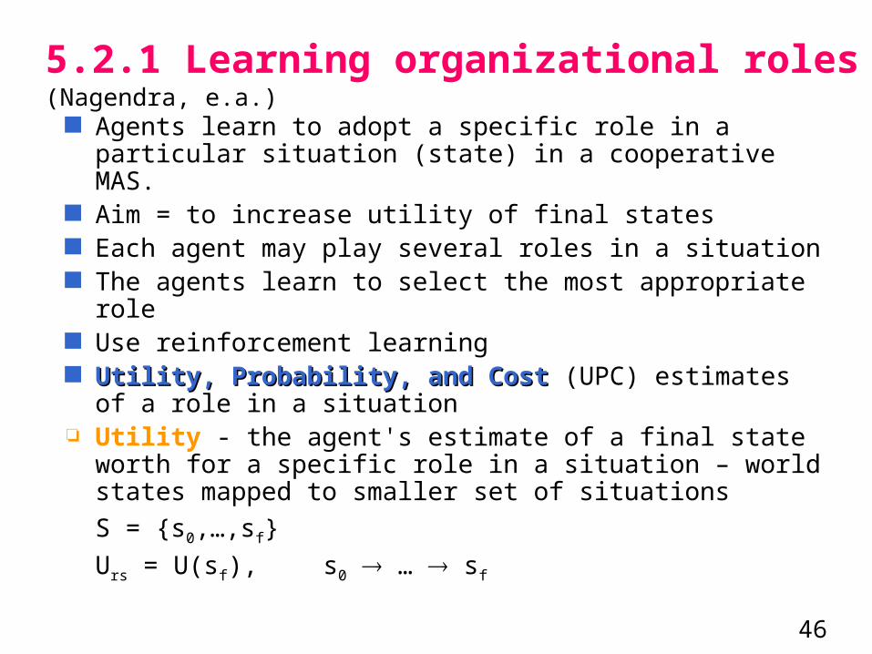
Agents learn to adopt a specific role in a particular situation (state) in a cooperative MAS.

Aim = to increase utility of final states Each agent may play several roles in a situation The agents learn to select the most appropriate role Use reinforcement learning Utility, Probability, and CostUtility, Probability, and Cost (UPC) estimates of a role

in a situation Utility - the agent's estimate of a final state worth for a

specific role in a situation – world states mapped to smaller set of situations

S = {s0,…,sf}

Urs = U(sf), s0 … sf

46

5.2.1 Learning organizational roles (Nagendra, e.a.)

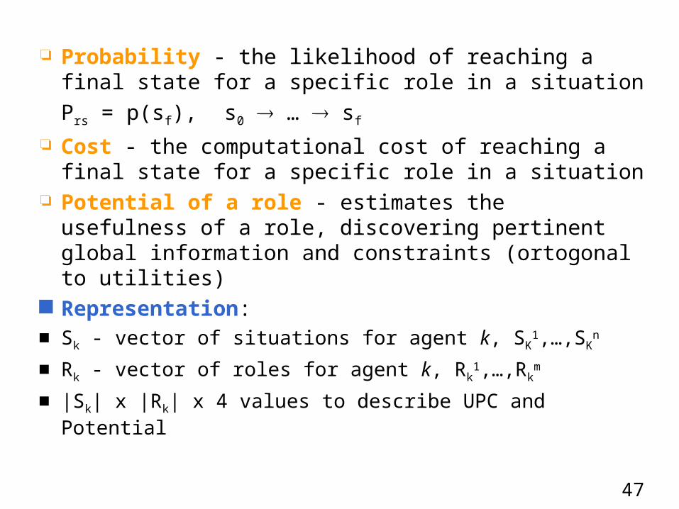
Probability - the likelihood of reaching a final state for a specific role in a situation

Prs = p(sf), s0 … sf

Cost - the computational cost of reaching a final state for a specific role in a situation

Potential of a role - estimates the usefulness of a role, discovering pertinent global information and constraints (ortogonal to utilities)

Representation: Sk - vector of situations for agent k, SK

1,…,SKn

Rk - vector of roles for agent k, Rk1,…,Rk

m

|Sk| x |Rk| x 4 values to describe UPC and Potential47

FunctioningFunctioning

Phase I: Learning

Several learning cycles; in each cycle:

each agent goes from s0 to sf and selects its role as the one with the highest probability

Probability of selecting a role r in a situation s

f - objective function used to rate the roles

(e.g., f(U,P,C,Pot) = U*P*C + Pot)

- depends on the domain

48

kRjjsjsjsjs

rsrsrsrsr PotCPUf

PotCPUfrP

),,,(

),,,()(

Use reinforcement learning to update UPC and the potential of a role

For every s [s0,…,sf] and chosen role r in s

Ursi+1 = (1-)Urs

i + Usf

i - the learning cycle

Usf - the utility of a final state

01 - the learning rate

Prsi+1 = (1-)Prs

i + O(sf)

O(sf) = 1 if sf is successful, 0 otherwise

49

50

Potrsi+1 = (1-)Potrs

i + Conf(Path)

Path = [s0,…,sf]

Conf(Path) = 0 if there are conflicts on the Path, 1 otherwise

The update rules for cost are domain dependent

Phase II: Performing

In a situation s the role r is chosen such that:

),,,(arg max jsjsjsjsRj

PotCPUfrk

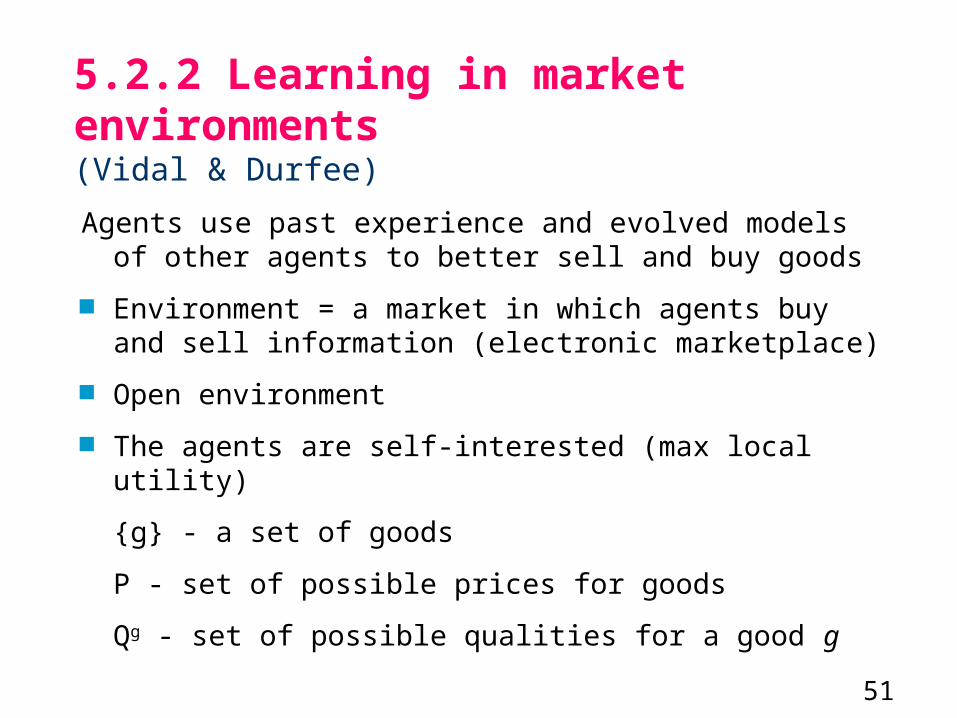
Agents use past experience and evolved models of other agents to better sell and buy goods

Environment = a market in which agents buy and sell information (electronic marketplace)

Open environment

The agents are self-interested (max local utility)

{g} - a set of goods

P - set of possible prices for goods

Qg - set of possible qualities for a good g51

5.2.2 Learning in market environments(Vidal & Durfee)

information has a cost for the seller and a value for the buyer information is sold at a certain price a buyer announces a good it needs sellers bid their prices for delivering the good the buyer selects from these bids and pays the corresponding price the buyer assesses the quality of information after it receives it from

the seller ProfitProfit of a seller s for selling the good g at price p

Profitsg(p) = p - cs

g

csg - the cost of producing the good g by s; p - the

price ValueValue of a good g for a buyer b

Vbg(p,q) p - price b paid for g

q - quality of good g

GoalGoal seller - maximize profit in a transaction buyer - maximize value in a transaction

52

3 types of agents3 types of agents

0-level agents0-level agents they set their buying and selling prices based on their

own past experience they do not model the behavior of other agents

1-level agents1-level agents model other agents based on previous interactions they set their buying and selling prices based on these

models and on past experience they model the other agents as 0-level agents

2-level agents2-level agents same as 1-level agents but they model the other agents

as 1-level agents53

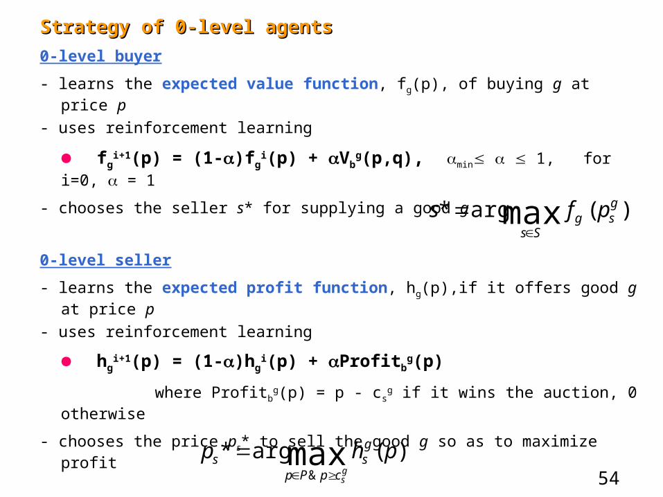
Strategy of 0-level agentsStrategy of 0-level agents

0-level buyer

- learns the expected value function, fg(p), of buying g at price p

- uses reinforcement learning

fgi+1(p) = (1-)fg

i(p) + Vbg(p,q), min 1, for i=0, = 1

- chooses the seller s* for supplying a good g

0-level seller

- learns the expected profit function, hg(p),if it offers good g at price p

- uses reinforcement learning

hgi+1(p) = (1-)hg

i(p) + Profitbg(p)

where Profitbg(p) = p - cs

g if it wins the auction, 0 otherwise

- chooses the price ps* to sell the good g so as to maximize profit

54

)(arg* max gsg

Ss

pfs

)(arg* max&

php gs

cpPps

gs

Strategy of 1-level agentsStrategy of 1-level agents

1-level buyer

- models sellers for good g

- does not model other buyers

- uses a probability distribution function qsg(x) over the qualities x of a

good g

- computes expected utility, Esg, of buying good g from seller s

- chooses the seller s* for supplying a good g that maximizes this expected utility

55

gs

Ss

Es maxarg*

Qx

gs

gb

gs xpVxq

QE ),()(

1

1-level seller

- models buyers for good g- models the other sellers s for good g Buyer's modeling

- uses a probability distribution function mbg(p) - the probability that

b will choose price p for good g Seller's modeling

- uses a probability distribution function ns'g(y) - the probability that

s' will bid price y for good g- computes the probability of bidding lower than a given seller s'

with the price pProb_of_bidding_lower_than_s' =

p'(Prob of bid of s' with p' for which s wins) =

p' N(g,b,s;s',p,p')

N(g,b,s;s',p,p') = ns'g(p') if mb

g(p') mbg(p)

0 otherwise56

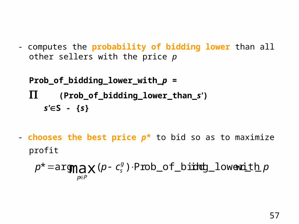
- computes the probability of bidding lower than all other sellers with the price p

Prob_of_bidding_lower_with_p =

(Prob_of_bidding_lower_than_s')

s'S - {s}

- chooses the best price p* to bid so as to maximize profit

57

pcpp gs

Pp

_withing_lower_ob_of_biddPr)(arg* max

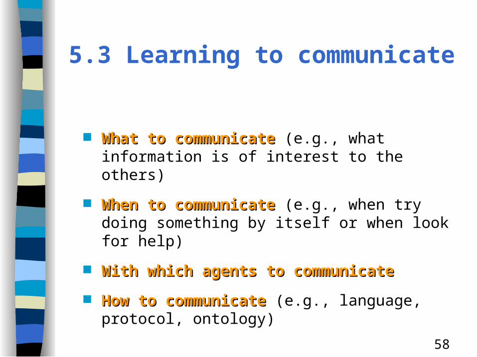
What to communicateWhat to communicate (e.g., what information is of interest to the others)

When to communicateWhen to communicate (e.g., when try doing something by itself or when look for help)

With which agents to communicateWith which agents to communicate

How to communicateHow to communicate (e.g., language, protocol, ontology)

58

5.3 Learning to communicate

Learning to which agents to ask for performing a task Used in a contract net protocol for task allocation to

reduce communication for task announcement Goal = acquire and refine knowledge about other agents'

task solving abilities Case-based reasoning used for knowledge acquisition

and refinement

A case consists of:

(1) A task specification

(2) Information about which agents solved a task or similar tasks in the past and the quality of the provided solution

59

Learning with which agents to communicate (Ohko, e.a. )

(1) Task specification

Ti = {Ai1 Vi1, …, Aimi Vimi}

Aij - task attribute, Vij - value of attribute Similar tasks

Sim(Ti, Tj) = r s Dist(Air, Ajs)

AirTi, AjsTj

Dist(Air, Ajs) = Sim_Attr(Air, Ajs) * Sim_Vals(Vir, Vjs)

Set of similar tasks

S(T) = {Tj : Sim(T, Tj) 0.85}

60

(2) Which agents performed T or similar tasks in the past

Suitability of Agent k

Perform(Ak, Tj) - quality of solution for Tj assured by agent Ak performing Tj in the past

The agent computes

{ Suit(Ak, T), Suit(Ak, T)>0 } and selects the agent k* such that

or the first m agents with best suitability

After each encounter, the agent stores the tasks performed by other agents and the solution quality

Tradeoff between exploitation and exploration

61

)(

),()(

1),(

TSTjkk

j

TAPerformTS

TASuit

),(arg* max TASuitk kk

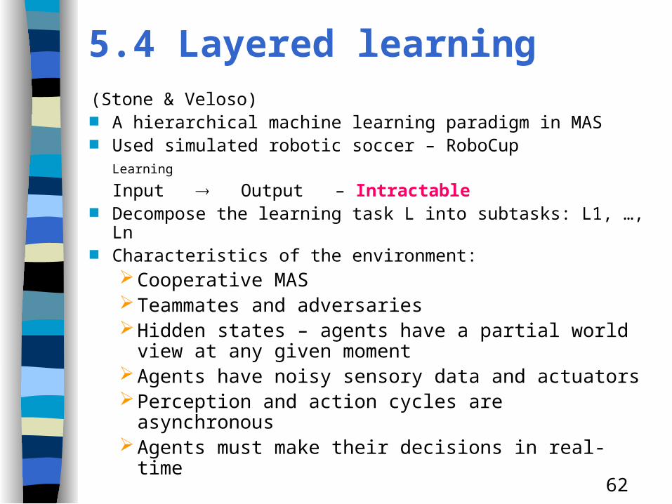
(Stone & Veloso) A hierarchical machine learning paradigm in MAS Used simulated robotic soccer – RoboCup

Learning

Input Output – Intractable Decompose the learning task L into subtasks: L1, …, Ln Characteristics of the environment:

Cooperative MASTeammates and adversariesHidden states – agents have a partial world view

at any given momentAgents have noisy sensory data and actuatorsPerception and action cycles are asynchronousAgents must make their decisions in real-time

62

5.4 Layered learning

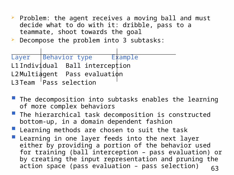
Problem: the agent receives a moving ball and must decide what to do with it: dribble, pass to a teammate, shoot towards the goal

Decompose the problem into 3 subtasks:

Layer Behavior type ExampleL1 Individual Ball interceptionL2 Multiagent Pass evaluationL3 Team Pass selection

The decomposition into subtasks enables the learning of more complex behaviors

The hierarchical task decomposition is constructed bottom-up, in a domain dependent fashion

Learning methods are chosen to suit the task Learning in one layer feeds into the next layer either by providing a

portion of the behavior used for training (ball interception – pass evaluation) or by creating the input representation and pruning the action space (pass evaluation – pass selection)

63

L1 – Ball interceptionL1 – Ball interceptionbehavior = individual

Aim:Blocks or intercepts opponents shots or passes orReceive passes from teammates

Learning methodLearning method: a fully connected backpropagation NN

Repeatedly shooting the ball towards a defender in front of a goal.The defender collects t.e. by acting randomly and noticing when it successfully stops the ball

Classification:Saves = successful interceptionsGoals = unsuccessful attemptsMisses = shoots that went wide of the goal

64

L2 – Pass evaluationL2 – Pass evaluationbehavior = multiagent

Uses its learned ball-interception skills as part of the behavior for training MAS behavior

Aim: the agent must decide To pass (or not) the ball to a teammate and If the teammate will successfully receive the ball (based on

positions + abilities of the teammate to receive or intercept a pass) Learning methodLearning method: decision trees (C4.5) Kick the ball towards randomly placed teammates interspread with

randomly placed opponents The intended pass recipient and the opponents all use the learned ball-

interception behavior Classification of a potential pass to a receiver:

Success, with a c.f. (0,1] Failure, with a c.f. [-1,0) Miss, (= 0)

65

L3 – Pass selectionL3 – Pass selectionbehavior = team

Uses its learned pass-evaluation capabilities to create the input and output set for learning pass selection

Aim: the agent has the ball and must decide To which teammate to pass the ball or Shoot on goal

Learning methodLearning method: Q-learning of a function that depends on the agent’s position on the field

Simulate 2 teams playing with identical behavior others than their pass-selection policies

Reinforcement = total goals scored Learns:

Shoot the goal The teammate to which to pass

66

There is no unique method or set of methods for learning in MAS

Many approaches are based on extending ML techniques in a MAS setting

Many approaches use reinforcement learning, but also NN or genetic algorithms

67

6 Conclusions6 Conclusions

ReferencesReferences S. Sen, G. Weiss. Learning in Multiagent systems. In Multiagent

Systems - A Modern Approach to Distributed Artificial Intelligence, G. Weiss (Ed.), The MIT Press, 2001, p.257-298.

T. Ohko, e.a. - Addressee learning and message interception for communication load reduction in multiple robot environment. In Distributed Artificial Intelligence Meets Machine Learning, G. Weiss, Ed., Lecture Notes in Artificial Intelligence, Vol. 1221, Springer-Verlag, 1997, p.242-258.

M.V. Nagendra, e.a. Learning organizational roles in a heterogeneous multi-agent systems. In Proc. of the Second International Conference on Multiagent Systems, AAAI Press, 1996, p.291-298.

J.M. Vidal, E.H. Durfee. The impact of nested agent models in an information economy. In Proc. of the Second International Conference on Multiagent Systems, AAAI Press, 1996, p.377-384.

P. Stone, M. Veloso. Layered Learning, Eleventh European Conference on Machine Learning, ECML-2000.

68

Web ReferencesWeb References An interesting set of training examples and the connection between decision

trees and rules.

http://www.dcs.napier.ac.uk/~peter/vldb/dm/node11.html Decision trees construction

http://www.cs.uregina.ca/~hamilton/courses/831/notes/ml/dtrees/4_dtrees2.html Building Classification Models: ID3 and C4.5

http://yoda.cis.temple.edu:8080/UGAIWWW/lectures/C45/        Introduction to Reinforcement Learning

http://www.cs.indiana.edu/~gasser/Salsa/rl.html

        On-line book on Reinforcement Learning

http://www-anw.cs.umass.edu/~rich/book/the-book.html

69