mathematical modeling of electromagnetic wave

Progress In Electromagnetics Research, PIER 37, 129–141, 2002

MATHEMATICAL MODELING OFELECTROMAGNETIC WAVE SCATTERING BY WAVYPERIODIC BOUNDARY BETWEEN TWO MEDIA

J. Chandezon

Universite Blaise Pascal LASMEA24 Ave. des Landais, 63167, Clermont-Ferrand, France

A. Ye. Poyedinchuk, Yu. A. Tuchkin†, and N. P. Yashina‡

Institute of Radiophysics and ElectronicsNational Academy of Sciences of Ukraine12, Ak. Proskury St., Kharkov, 61085, Ukraine

Abstract—The extension of C method, combined with idea ofTikhonov’s regularization is proposed. The regularizing algorithm fornumerical solution of electromagnetic wave diffraction by the boundaryof dielectric media is developed. This algorithm is based on the solutionof the system linear algebraic equations of C method as subject ofregularizing method of A. N. Tikhonov. The numerical calculationsof scattered field in the case of E-polarization are presented. Theefficiency and reliability of the method for the solution of the problemsof boundary shape reconstruction have been proved and demonstratednumerically for several situations.

1 Introduction

2 Direct Problem

3 Spectral Problem of C-Method

4 The Solution to the Diffraction Problem. RegularizingAlgorithm

5 Inverse Problem† Also with Gebze Institute of Technology, PK. 141, 41400 Gebze-Kocaeli, Turkey‡ Also with Universite Blaise Pascal LASMEA, 24 Ave. des Landais, 63167, Clermont-Ferrand, France

130 Chandezon et al.

6 Numerical Experiments

7 Conclusion and Perspective

References

1. INTRODUCTION

Mathematical modeling for boundaries between two media (terrainsurface, ocean) has a large history and bibliography [1–4].

An efficient remote terrain and ocean monitoring requires solvingof the following problems. The first, direct one, is the development ofelectromagnetic models of electromagnetic waves scattering by surfacesof various media. The second, inverse one, is based on these modelsand has to provide estimation and remote control of the relief of oceanand earth, namely their properties relying on information about certaincharacteristics of scattered electromagnetic fields.

It is clear that an efficient and robust solution to direct problemmentioned above is of principal importance. Although huge bodyof papers treating this complicated problem, there is evident lack ofsolutions which are based on rigorous approaches.

We propose here the robust and clear in implementation methodthat present certain modification of known C method [5–10] for solvingthe problem of electromagnetic wave scattering by rather arbitraryshaped surface. This approach makes a reliable base for solution ofrecognition problem: the reconstruction of surface profile and materialparameters of media from known data of scattered electromagneticfield.

The major objective of present paper is consideration of theprincipal methodological issues, which can testify an accuracy andefficiency of the solution, and serve as keys to the successful utilizationof the method suggested in real life experiments and devises. Thepreliminary study demonstrates high performance and reliability ofthe approach for rather wide scope of problems of material parametersand surface relief recognition and reconstruction.

2. DIRECT PROBLEM

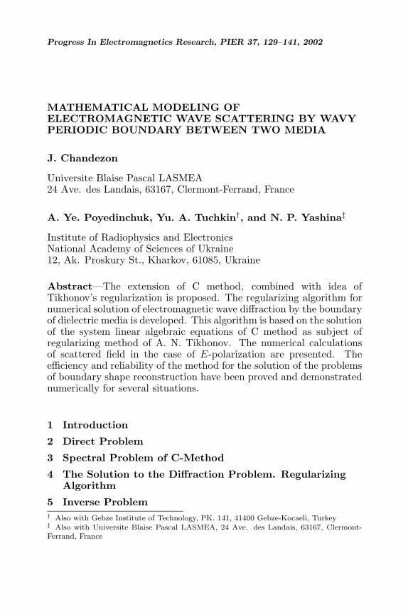
We consider two dimensional diffraction problem for time-harmonicE polarized (electric field density vector is parallel to axis 0x) planewaves by the arbitrary profile boundary of two media with relativepermittivities ε1 and ε2 and permeability µ (Fig. 1). The boundaryline between two media is described by function z = a (y) with period

Mathematical modeling of electromagnetic wave 131

2ε

ϕ

1ε

z

y

d

h

I

II

Figure 1. The profile of boundary between two media.

d, maximal deviation from axis 0y is equal to h (see Fig. 1). Incidentplane wave propagates in the media with permittivity ε1 with angle ofincidence ϕ, which is counted as shown in Fig. 1. Time factor is chosenas e−iωt. The excitation fields has the form

H iy = Aei2πλ

√ε1µ(y sin(ϕ)−z cos(ϕ))

H iy = −√ε1µ

cos (ϕ)Eix

H iz = −√ε1µ

sin (ϕ)Eix

Here λ is a wavelength in vacuum.It is necessary to find out the diffraction filed that has to meet

fallowing requirements:

1. Maxwell equations;2. Radiation conditions at infinity;3. Transparency boundary conditions, requiring continuity of

tangential components of total field in the boundary;4. The quasi periodic conditions (Floquet conditions);5. The condition of energy boundness in any finite domain.

It can be proved, (see, for example [11] and [12]) that conditions 1–5 guarantee the unique-ness of the diffraction problem solution. Forfurther convenience we introduce the following variables:

z = κz, y = κy, κ = 2π/d.


Then Maxwell equations for diffraction field acquire the form

∂Esxn∂z

= ikµHsyn

−∂Esxn

∂y= ikµHszn

−ikεnEsxn =∂Hszn∂y

−∂Hsyn∂z

n = 1, 2; (1)

where κ = d/λ, values n = 1 and n = 2 refer to the first and secondmedia. The equation defining the boundary between media in newvariables can be presented in the following form

z = A0a (y) , A0 = 2πh/d,

where a (y) is a periodic function with period equals 2π such that0 ≤ a (y) ≤ 1.

For the sake of simplicity we consider the case ϕ = 0. Allderivations for the case ϕ �= 0 can be obtained in the similar way.

Subjecting diffraction field to boundary conditions, we derive

−iκ1e−iκ1A0a(y) +

∂Esx1

∂z−A0a (y)

∂Esx1

∂y=

∂Esx2

∂z−A0a (y)

∂Esx2

∂y

e−iκ1A0a(y) + Esx1= Esx2

(2)

where κ1 = κ√ε1µ. Notation like a (y) means here and below the

derivation in respect to the argument.Following the conventional C method, we introduce new variables

v = y, u = z −A0a (y), which transform equation (1) into the form

(∂

∂v−A0a (v)

∂

∂u

)G1n +G2n = 0,

−(∂2

∂u2+ κ2εnµ

)G1n +

(∂

∂v−A0a (v)

∂

∂u

)G2n = 0,

n = 1, 2;

(3)where G1n = Esxn, G2n = iκµHszn. The equation, describing boundary,simplifies itself into u = 0 and transforms the boundary condition intoequations

−iκ1e(−iκ1A0a(v)) +

(1 +A2

0a2) ∂G11

∂u−A0a

∂G11

∂v

=(1 +A2

0a2) ∂G12

∂u−A0a

∂G12

∂v(4)


e(−iκ1A0a(v)) +G11 (v, 0) = G12 (v, 0)

The further derivations are connected with transformation of (3)and (4) into infinite system of linear algebraic equations with respectto unknown coefficients, which are the coefficients of expansions offunctions G11, G12 over the system of eigen functions of relevantspectral problems of C method.

3. SPECTRAL PROBLEM OF C-METHOD

We are seeking for the solutions of (3) having the form

Gn = eiρnugmn (v) ,m, n = 1, 2 (5)

where ρn are the spectral parameters of C method. After substitutionof (5) into (3) we arrive to

{g1n − iρA0a (v) g1n + g2n = 0

g2n − iρA0a (v) g2n +(ρ2n − κ2εnµ

)g1n = 0

n = 1, 2 (6)

It is easy to see that functions g1n and g2n satisfy the equation

−gmn + 2iρA0agmn +[iρA0a+ ρ2A2

0a2 + ρ− k2εnµ

]gmn = 0 (7)

As a solution to (3) has to be periodic function with respect to variablev, the periodic condition is to be fulfilled by functions gmn (v):

gmn (0) = gmn (2π) , gmn (0) = gmn (2π) (8)

Hence, it is necessary to find out the values of spectral parameter pproviding non trivial solutions to equation (7) meeting the periodicitycondition (8). The solution to this problem can be constructed in thefollowing way. We shall seek for functions gmn (v) as an expansion toFourier series:

gmn (v) =∞∑

p=−∞Fmnp eipv (9)

Substituting (9) into (6) we obtain the infinite system of equationsthat we can present in matrix form

X −An (ρ)X = 0 (10)

whereX =

∥∥∥∥ F1n

F2n

∥∥∥∥ , Fnm =(Fnmp

)∞p=−∞


An (ρ) =[A (ρ) −iDiγ2nD A (ρ)

], A (ρ) = ‖Aqp‖∞q,p=−∞

D = ‖Dqp‖∞q,p=−∞ , Dqp =

1, p = q = 0δqpp, p �= 0

and δqp is Kroneker delta, γ2n = κ2εnµ − ρ2. The entries Aqp are

expressed via Fourier coefficients of function a (v):

Aqp =

1, p = q = 0

ρA0a−p, q = 0

ρA0aq−pq, q �= 0

Matrices A (ρ) and D produce compact operators in space l2,which are analytically depending on spectral parameter p. Thus,matrices An (ρ) from (10) also produce compact operator in spacel2 × l2, and each An (ρ) is analytical operator-function of parameterp.

It can be proved that for ρ �= ±√κ2εnµ− p2, where p =

0,±1,±2..., the bounded operator (I−An (ρ))−1 exists. The set ofvalues p, providing the existence of nontrivial solutions to equation(10), is countable, isolated and of finite multiplicity. This followsfrom Fredholm’s theorem [13] about analytical operator-functions. Fornumerical solution of (10) we applied truncation method. This iscorrect for operator-function An (ρ) is compact.

Now, having values of spectral parameter p and corresponding to peigen vectors X, one can construct the functions eiρugmn (v), satisfyingthe system of equations (3).

4. THE SOLUTION TO THE DIFFRACTION PROBLEM.REGULARIZING ALGORITHM

As it has been stated above, the set of spectral parametercorresponding to both media (n = 1, 2) is not more than countableand isolated set.

Let Un = (ρmn)∞,m=1 n = 1, 2 is the set of spectral parameters such

that Re (ρm1) + Im (ρm1) ≥ 0 and Re (ρm2) + Im (ρm2) ≤ 0. Then,according to C-method, functions G11 and G12, describing diffractionfields in the first and second media correspondingly, can be presented


in the formG11 =

∑m∈V1

Cm1eiρm1ugm1(ν), u ≥ 0

G12 =∑m∈V1

Cm2eiρm2ugm2(ν), u ≤ 0

(11)

Note, that the choice of sets Un, n = 1, 2 is dictated by necessityfor diffraction field to meet radiation conditions in correspondingdomains - half spaces u ≥ 0 and u ≤ 0 respectively. Now, we substituteexpansion (11) into boundary conditions (4), and accounting (9), weobtain the finite system of linear algebraic equations with unknowns(Cnm)∞m=−∞ , n = 1, 2,∑

m∈U1

Fm1n Cm1 −

∑m∈U2

Fm2n Cm2 = −Ln (−A0κ1) (12)

∑m∈U1

Gm1n Cm1 −

∑m∈U2

Gm2n Cm2 = κ1Ln (−A0κ1)

n = 0,±1,±2 . . . (13)

Here

Gmpn =κ2εpµ− n2

ρmpFmpn + nA0

+∞∑s=−∞

an−sFmps

Ln(γ) =12π

2π∫0

exp{iγa(ν)− inν}dν (14)

an =12π

2π∫0

a(ν) exp{−inν}dν

We can also rewrite (12) in matrix form:

Fx = B, F =[F1 −F2

G1 −G2

]

Fp = ‖Fmpn ‖∞m=1,n=−∞ , Gp = ‖Gmpn ‖∞m=1,n=−∞

B =∥∥∥∥ B1

B2

∥∥∥∥ , B1 = (−Ln (−κ1A0))∞n=−∞

B2 = −κ1B1, x =∥∥∥∥ C1

C2

∥∥∥∥

(15)

Analyses of matrix entries of (12) made it clear that operatorequation (14) is an equation of the first kind. That is why the direct


usage of truncation method for numerical solution of (14) is undesirablebecause of well known instability problem arising. That is why someregularizing procedure is absolutely necessary. We suggest to solveoperator equation (14) applying Tikhonov’s regularization [14].

The formal schema of regularizing procedure includes the followingsteps. Owing to the fact that original diffraction problem has uniquesolution, equation (14) has unique solution also. Suppose that insteadof explicit values of F and B we know their approximate values F andB, namely

sup‖x‖=1

∥∥∥F x− Fx∥∥∥ ≤ h, ∥∥∥B −B∥∥∥ ≤ δwhere h and δ are known input data of the algorithm.

As F and B we can take corresponding truncated matrixes in(12). Tikhonov’s regularization method suggest the search of elementsxα providing minimum to smoothing functional

Φα (xα) =∥∥∥F xα − B∥∥∥2

+ α ‖xα‖2 (16)

where α > 0 is regularizing parameter, which is to be defined from thecondition ∥∥∥F xα − B∥∥∥2

= 2(h ‖xα‖2 + δ

)(17)

As a norm ‖. . .‖ in (15) one can choose the norm of correspondingfinite-dimensional space. With such a choice the search of xα from(15) is equivalent to the solution of the equation

αxα + F ∗F xα = F ∗B (18)

Here F ∗ is the conjugate to F operator.Equation (17) has been solved numerically by means of truncation

method. Parameter α has been chosen from condition (16). Numericalexperiments proved high efficiency and considerable enforcing ofstability of the suggested method of the solution to (14).

5. INVERSE PROBLEM

The developed above method of the solution to the direct diffractionproblem and corresponding numerical algorithm form the efficientbackground for the following inverse problem.

The input data for the problem are complex amplitudes R =(Rn (λ))Nn=−N of reflected propagating waves, λ is a wave length. We


suppose that this data are known in certain range [λ1, λ2]. Besides theperiod of boundary shape and dielectric parameters of media are alsoknown. It is necessary do find out by these input data the function,defining the boundary of two media. Let a = (an)

∞n=−∞ are Fourier

coefficients of this boundary function. The solutionof operator equation (17) gives the mapping that associates set

of a = (an)∞n=−∞ with set of complex amplitudes R = (Rn (λ))Nn=−N .

Thus, the non linear operator

F (a, λ) = R (λ) , λ ∈ [λ1, λ2] (19)is defined on certain set of vectors DF ⊂ l2. Consequently, the

mathematical posing of inverse problem consists in finding out thesolution to (18) in such sense that residual F (a, λ)−R (λ) is minimizedin relevant metric (see (20) ). Having found out the Fourier coefficientsa = (an)

∞n=−∞ from (18), we can derive the function, describing the

boundary between two media. This can be done by means of stableprocedure that is the summation of Fourier series with approximate inl2 space metric coefficients [15].

Formally, the scheme of solution may be outlined as follows. LetY (λ) is the set of operator F values. Introduce on Y (λ) the normaccording to the following formula

‖R (λ)‖21 =N∑−N|Rn (λ)|2 cosϕn

cosϕ(20)

Here the following notations are used: ϕn are angles of diffracted field,ϕ is angle of the incident field. Consider the functional that is givenin domain DF of operator F definition:

Φ (a) =P∑m=1

∥∥∥Ren (λm)−RMn (λm)∥∥∥2

1+ γ

Q∑n=−Q

|an|2(1 + n2R

)(21)

where γ > 0 is the parameter of regularization, R = 1 (in general,R ≥ 1 is a parameter of the functional), λm ∈ [λ1, λ2] , a (y) =Q∑

n=−Qane

iny, . Vector ay = (aγn)Qn=−Q, which provides the functional

(20) with minimum, is considered to be a solution to (18). Norm ‖. . .‖1is defined by formula (19). Vectors Re = (R (λm))Pm=1 are input dataof inverse problem. They can be found from solution of direct problem(12) with given vector ay = (aγn)

Qn=−Q.

The search of vector ay is constructed by means of regularizedquasi Newton’s method with step adjustment, using only first


derivatives. The minimum residual method (see [14,15]) is applied forthe choice of regularizing parameter γ that is in compliance with givenlevel of noise in input data Re (λm) = (Ren (λm))Nn=−N . On the bases ofthe approach developed, the numerical algorithms for the solving (18)and (19) have been implemented.

6. NUMERICAL EXPERIMENTS

Here we present several numerical illustrations for test problems, whichhave been performed by suggested approach and the correspondingalgorithm implementation. Relying on the solution to equation (17),we simulated input data Re (λm) = (Ren (λm))Nn=−N , m = 1, 2 . . . Pfor two boundaries between media. We have chosen two types ofboundary profile:

a1 (y) = h

[0.5 +

π3y

6d

(2yd− 1

) (1− y

d

)]

and

a2 (y) = h[0.375 + 0.25 sin

(2πyd

)+ 0.125 cos

(4πd

)]

that are periodically continued from interval [0, d] onto interval(−∞,+∞). Parameters d and h feet restriction 2πh

d ≤ 1. Thewavelength of incident plane E polarized wave was varying within therange 0.5 ≤ d

λ ≤ 3.5. Permittivity of the first medium has been chosenas ε1 = 1 and of the second one as ε2 = 2.25. Permeability of bothmedia is µ = 1. Functions a1 (y) and a2 (y) are chosen for they belongto two essentially different classes. Namely, function a2 (y) is a finiteseries of its Fourier coefficients. In the contrary, function a1 (y) is aninfinite Fourier series, which Fourier coefficients have algebraic type ofdecaying only.

Results of numerical tests are presented in Fig. 2 and Fig. 3. Solidlines correspond to the ex-act functions a1 (y) and a2 (y). Dottedlines are the graphs of functions aR1 (y) and aR2 (y) that have beendefined via input data Re (λm) = (Ren (λm))Nn=−N according to abovedescribed algorithm. As they almost coincide with graphic accuracy,the deviations h−1

(∣∣∣a1 (y)− aR1 (y)∣∣∣) and h−1

(∣∣∣a21 (y)− aR2 (y)∣∣∣) are

presented in the same figures. As it is clearly seen, the maximumabsolute value of deviation is less than 10−3 for function a2 (y) and10−2 for a1 (y). It worth to be emphasized that maximum absolutevalue of deviation essentially decreases with value of points P increases


0 1 2 3 4 5 6 70

0.1

0.2

0.3

0.4

0.5

0.6

0.7

0.8

0.9

1

P =36

a(y)reconstrdeviation*10

0 1 2 3 4 5 6 70

0.1

0.2

0.3

0.4

0.5

0.6

0.7

0.8

0.9

1

a(y)reconstrdeviation*10

dyπ2 dyπ2a) b)

P =6

Figure 2. Reconstruction of boundary shape for the profile given byfunction a1(y) = h

[0.5 + π3y

6d

(2yd − 1

) (1− y

d

)]for different values P

of given incident waves: P = 6 (Fig. a) and P = 36 (Fig. b), whereε2 = 2.25, 0.5 ≤ d/λ ≤ 3.5, 2πh/d = 0.4.

0 1 2 3 4 5 6 70

0.1

0.2

0.3

0.4

0.5

0.6

0.7reconstructeddeviation*100a(y)

0 1 2 3 4 5 6 7-0.1

0

0.1

0.2

0.3

0.4

0.5

0.6a(y)reconstructeddeviation*100

dyπ2dyπ2

a) b)

P =6 P =36

Figure 3. Reconstruction of boundary shape for the profile givenby function a1(y) = h

[0.375 + 0.25 sin

(2πyd

)+ 0.125 cos

(4πd

)]for

different values P of given incident waves: P = 6 (Fig. a) and P = 36(Fig. b), where ε2 = 2.25, 0.5 ≤ d/λ ≤ 3.5, 2πh/d = 0.4.

(we remind that P is a number of values of incident plane wavewavelengths, for which the input data Re (λm) , m = 1, 2 . . . P havebeen calculated).

Basing on the numerical experiments have been performed andpartially illustrated here, we can conclude that the approach suggestedenables the reconstruction of the boundary functions of two media.When the relative level of noise in input data is about 10−3, the relativeerror of the profile reconstruction is less than 10−2.


7. CONCLUSION AND PERSPECTIVE

The extension of C method is suggested. It is made in two maindirections. The first one is concerning direct two dimensional problemof time-harmonic plane wave diffraction by periodic boundary betweentwo dielectric media. The key new step is Tikhonov’s regularizationinvolved in solution procedure. Such involving has given essentialincreasing of the stability of canonic C method.

The second extension is based on the first one, and is devoted tonew area of C method application, namely, to inverse and ill posedproblems of various media’s boundary recognition and reconstruction.This extension, as well as the first one, includes ideas of Tikhonov’sregularization as essential part of the method.

Numerical tests proved the efficiency and rather good stabilityof new algorithms suggested. A very similar technique can be usedfor reconstruction of material parameters of the media (which weresupposed to be known in the present paper). The detailed descriptionof such aimed algorithms will be the topic of our special publication.

Thus, the methods developed herein and, especially, the ideaslying in their background are looking very promising for the solutionof wide area of applied problems of remote sensing and monitoring ofearth and ocean.

REFERENCES

1. Van Oevelen, P. and D. Hoekman, “Radar backscatter inversiontechnique for estimation of surface soil moisture: EFEDA–Spain and HAPEX-Sahel case studies,” IEEE Transactions onGeoscience and Remote Sensing, Vol. GE-37, p. I, No. 1. 113–124, 1999.

2. Njoku, E. G., Y. Rahmat-Samii, J. Sercel, W. J. Wilson, andM. Maghaddam, “Evaluation of an inflatable antenna conceptfor microwave sensing of soil moisture and ocean salinity,” IEEETransactions on Geoscience and Remote Sensing, Vol. GE-37, p. I,No. 1, 79–94, 1999.

3. Njoku, E. G. and L. Li, “Retrieval of land surface parametersusing passive micro wave measurements at 6–18 GHz,” IEEETransactions on Geoscience and Remote Sensing, Vol. GE-37, p. I,No. 1, 63–79, 1999.

4. Ostrov, D. N., “Boundary conditions and fast algorithms forsurface reconstruction from Synthetic aperture radar data,” IEEETransactions on Geoscience and Remote Sensing, Vol. GE-37,p. II, No. 1, 335–346, 1999.


5. Li, L., J. Chandezon, G. Granet, and J.-P. Plumey, “A rigorousand efficient grating analysis method made easy for opticalengineers,” Journal of Optical Society of America, No. 1, 1999.

6. Plumey, J.-P., B. Guizal, and J. Chandezon, “Coordinatetransformation method as applied to asymmetric gratings withvertical facets,” Journal of Optical Society of America, No. 3,1997.

7. Granet, G., J.-P. Plumey, and J. Chandezon, “Some topics inextending the C method to multilayer-coated gratings of differentprofiles,” Pure Appl. Opt., No. 2, 1996.

8. Plumey, J.-P., G. Granet, and J. Chandezon, “Differentialcovariant formalism for solving Maxwell’s equations in curvilinearcoordinates: oblique scattering from lossy periodic surfaces,”IEEE Trans. AP, AP 43, No. 8, 1995.

9. Chandezon, J., D. Maystre, and G. Raoult, “A new theoreticalmethod for diffraction gratings and its numerical application,”J.Optics (Paris), No. 4, 1980.

10. Chandezon, J., M. T. Depuis, G. Cornet, and D. Maystre,“Multicoated gratings: a differential formalism applicable in theentire optical region,” Journal of Optical Society of America,No. 7, 1982.

11. Petit, R. (ed.), Electromagnetic Theory of Gratings, Springer-Verlag, Heidelberg, 1980.

12. Shestopalov, V. P., L. N. Litvinenko, S. A. Masalov, andV. G. Sologub, Wave Diffraction by Gratings, Publ. of KharkovNational University, Kharkov, Ukraine, 1973.

13. Gohberg, I. Tz. and M. G. Krein, Introduction to the Theory ofLinear Non Self-Adjoined Operators in Hilbert Space, Moscow,Russia, 1965 (in Russian).

14. Tikhonov, A. N. and V. Ya. Arsenin, Methods for the Solution ofIll Posed Problems, Moscow, Russia, 1986.

15. Ivanov, V. K., V. V. Vasin, and V. P. Talanov, Theory of Linear IllPosed Problems and Its Applications, 208, Nauka, Moscow, Russia1978 (In Russian).

mathematical modeling of electromagnetic wave

Documents