modeling datalog assertion and retraction in linear logic

Modeling Datalog Assertion and Retraction inLinear Logic∗

Edmund S. L. Lam and Iliano Cervesato

June 2012CMU-CS-12-126

CMU-CS-QTR-113

School of Computer ScienceCarnegie Mellon University

Pittsburgh, PA 15213

Carnegie Mellon University, Qatar campus.

The author can be reached at [email protected] or [email protected].

Abstract

Practical algorithms have been proposed to efficiently recompute the logical consequences of a Datalogprogram after a new fact has been asserted or retracted. This is essential in a dynamic setting wherefacts are frequently added and removed. Yet while assertion is logically well understood as incrementalinference, the monotonic nature of first-order logic is ill-suited to model retraction. As such, the traditionallogical interpretation of Datalog offers at most an abstract specification of Datalog systems, but has tenuousrelations to the algorithms that perform efficient assertions and retractions in practical implementations.This report proposes a logical interpretation of Datalog based on linear logic. It not only captures themeaning of Datalog updates, but also provides an operational model that underlies the dynamic changes ofthe set of inferable facts, all within the confines of logic. We prove the correctness of this interpretation withrespect to its traditional counterpart.

∗ Funded by the Qatar National Research Fund as project NPRP 09-667-1-100 (Effective Programming for LargeDistributed Ensembles)

mailto:[email protected]

mailto:[email protected]

Keywords: Datalog, Linear Logic, Retraction, Assertion, Dynamic updates

CONTENTS

Contents

1 Introduction 1

2 Preliminaries 1

2.1 Notations . . . . . . . . . . . . . . . . . . . . . . . . . . . . . . . . . . . . . . . . . . . . . . . 1

2.2 Datalog . . . . . . . . . . . . . . . . . . . . . . . . . . . . . . . . . . . . . . . . . . . . . . . . 2

2.3 Linear Logic: LV obs and LV obs− . . . . . . . . . . . . . . . . . . . . . . . . . . . . . . . . . . 3

3 Example 4

4 Modeling Datalog Assertion 5

4.1 Inference Rules and Interpretation . . . . . . . . . . . . . . . . . . . . . . . . . . . . . . . . . 5

4.2 Quiescence and Complete Inference . . . . . . . . . . . . . . . . . . . . . . . . . . . . . . . . . 7

4.3 Correctness . . . . . . . . . . . . . . . . . . . . . . . . . . . . . . . . . . . . . . . . . . . . . . 8

5 Modeling Datalog Retraction 12

5.1 Retraction and Absorption Rules . . . . . . . . . . . . . . . . . . . . . . . . . . . . . . . . . . 12

5.2 Quiescence and Complete Retraction . . . . . . . . . . . . . . . . . . . . . . . . . . . . . . . . 14

5.3 The llDFull Interpretation . . . . . . . . . . . . . . . . . . . . . . . . . . . . . . . . . . . . . . 14

5.4 Cycles and Re-assertion . . . . . . . . . . . . . . . . . . . . . . . . . . . . . . . . . . . . . . . 15

5.5 Correctness . . . . . . . . . . . . . . . . . . . . . . . . . . . . . . . . . . . . . . . . . . . . . . 16

6 Related Work 23

7 Conclusions and Future Work 24

i

LIST OF FIGURES

List of Figures

1 Logical Specification of Datalog Updates . . . . . . . . . . . . . . . . . . . . . . . . . . . . . . 1

2 Syntax of Datalog . . . . . . . . . . . . . . . . . . . . . . . . . . . . . . . . . . . . . . . . . . 2

3 Fragment of the Intuitionistic Sequent Calculus, LJ . . . . . . . . . . . . . . . . . . . . . . . 3

4 LV obs and LV obs− Intuitionistic Linear Logic . . . . . . . . . . . . . . . . . . . . . . . . . . . 4

5 Example of Linear Logic Interpretation . . . . . . . . . . . . . . . . . . . . . . . . . . . . . . 5

6 LV obs− derivations of an example llDAssert interpretation . . . . . . . . . . . . . . . . . . . . 6

7 llDAssert Interpretation of Datalog . . . . . . . . . . . . . . . . . . . . . . . . . . . . . . . . . 6

8 llDAssert Inference Macro Rule . . . . . . . . . . . . . . . . . . . . . . . . . . . . . . . . . . . 7

9 An Example of llDFull− Interpretation with Assertion/Retraction Derivations . . . . . . . . . 8

10 An Example of llDFull Interpretation . . . . . . . . . . . . . . . . . . . . . . . . . . . . . . . . 12

11 llDFull Interpretation of Datalog . . . . . . . . . . . . . . . . . . . . . . . . . . . . . . . . . . 13

12 llDFull Inference Macro Rule . . . . . . . . . . . . . . . . . . . . . . . . . . . . . . . . . . . . 15

13 Assertion and Retraction, in llDFull . . . . . . . . . . . . . . . . . . . . . . . . . . . . . . . . 16

14 llDFull Retraction Macro Rule . . . . . . . . . . . . . . . . . . . . . . . . . . . . . . . . . . . 17

15 llDFull Absorption Macro Rule . . . . . . . . . . . . . . . . . . . . . . . . . . . . . . . . . . . 18

16 Example of Quiescence in the Presence of Cycles . . . . . . . . . . . . . . . . . . . . . . . . . 19

17 Example of re-assertion during retraction . . . . . . . . . . . . . . . . . . . . . . . . . . . . . 20

1

2 PRELIMINARIES

Assertion: P(B)+a

==⇒P P(B, a) Retraction: P(B, a)−a

==⇒P P(B)

where P(B) = {p(~t) | P,B ` p(~t)}.

Figure 1: Logical Specification of Datalog Updates

1 Introduction

Datalog, a logic programming language defined in the early 1980s, was originally used to describe andimplement deductive databases [GMN84]. Given a set B representing the data in the database, a Datalogprogram P specified recursive views that a user could then query. Logically, B is a set of ground atomicformulas (facts) and P a set of implicational formulas of a restricted form (Horn clauses). The semantics ofsuch a Datalog system, as well as some actual implementations [CGT89], was given by the set of the atomiclogical consequences of P with respect to B, in symbols {p(~t) | P,B ` p(~t)} — a beautifully pure use oflogic.

In the last ten years, Datalog has had a resurgence in a variety of domains other than databases: toprovide user authentication [LM03], to implement network protocols [GW10, LCG+06], to program cyber-physical systems [ARLG+09] and to support deductive spreadsheets [Cer07], just to cite a few. In theseapplications, the contents of the fact base B is highly dynamic, at least compared to the relatively staticdatabases of the 1980s. This requires efficient algorithms to assert new facts and to retract stale facts. Whilesuch algorithms have been proposed [ARLG+09, CARG+12, GMS93, LCG+06, NJLS11], the connection withlogic has lagged behind, especially for retraction. Indeed, although it is easy to give a logical specificationof assertion and retraction, as done in Figure 1, a direct implementation of these specifications is horriblyinefficient as it involves recomputing logical consequences from scratch after each assertion or retraction.

In this report, we propose a logical interpretation of Datalog that supports updates internally. Like withthe traditional reading, the semantics of a Datalog system (P, B) will be the set {p(~t) | P, B ` p(~t)} of itslogical consequences (plus some bookkeeping information). However, the assertion or retraction of a fact awill trigger a small number of logical inferences to determine the new set of logical consequences rather thanperforming a full recalculation. In this way, the proposed encoding not only constitutes a logical specificationof the static and dynamic aspects of a Datalog system, but it can also be viewed as an efficient algorithmto compute updates. Because retraction results in the removal of inferred facts, we base our encoding on afragment of first-order linear logic rather than on the traditional predicate calculus.

The main contributions of this report are therefore 1) the definition of an encoding of Datalog whichmodels the assertion and retraction of facts within logic, and 2) a proof of its correctness with respect to thetraditional interpretation.

The rest of this report is organized as follows: Section 2 reviews Datalog and linear logic. Section 3illustrates our approach with an example. Section 4 introduces an initial linear logic interpretation ofDatalog that focuses just on assertion. Section 5 extends it to capture retraction as well. We discuss relatedwork in Section 6, while Section 7 outlines directions of future work.

2 Preliminaries

This section provides a brief review of Datalog and linear logic. We first recall some common mathematicalnotions that we will use throughout this report.

2.1 Notations

In this report, we will refer to both sets and multisets. We write *a1, ..., an+ for a multiset with elementsa1, ..., an (possibly repeated) and S ] S′ for the multiset union of S and S′. We use ∅ to denote both theempty set and the empty multiset. Given a multiset S, we write set(S) for the set of the elements of S

1

2 PRELIMINARIES

Terms: t ::= x | cFacts: a, b, h ::= p(~t)

Clause: D ::= r : ∀~x. B ⊃ hClause bodies: B ::= b ∧B | b

Programs: P ::= D, P | ·Fact bases: B ::= p(~c), B | ·

Figure 2: Syntax of Datalog

(without duplicates). We write a for a generic set or multiset, disambiguating as needed. Sequences will bewritten as (a1, ..., an) or ~a, with ε for the empty sequence and S, S′ for the concatenation of two sequencesS and S′. A substitution [t1/x1, .., tn/xn], denoted θ, is a mapping of variables xi to terms ti. Given acollection S (set, multiset or sequence) of formulas and θ = [t1/x1, ..., tn/xn], we denotes with θ(S) thesimultaneous substitution of all free occurrences of xi in S with ti. We denote the set of free variables in Sas FV (S).

2.2 Datalog

Datalog is a declarative rule-based language, founded on traditional first-order logic. Its syntax is given inFigure 2. A Datalog system consists of a fact base, B, and a program, P. A fact base is a set of groundatomic formulas, called facts, of the form p(~c), where p is a predicate of fixed arity and ~c is a sequence ofconstants drawn from a fixed and finite signature Σ. A Datalog program is a set of clauses of the formr : ∀~x. b1 ∧ . . .∧ bn ⊃ h where h and bi are atomic formulas possibly mentioning variables among ~x, and r isa unique label acting as the rule’s name. We call h the head of r and b1 ∧ . . . ∧ bn its body. Datalog clausesare a restricted form of Horn clauses: the body cannot be empty, the arguments of each predicate must beeither constants or variables (function symbols are disallowed), and each variables in h must appear in theantecedent b1 ∧ . . . ∧ bn (variables are range-restricted). Furthermore, to keep the presentation simple, weshall assume that no two body atoms have common instances.

Datalog classifies predicates p into base predicates, whose values are supplied by the user and can appearonly in the body of a clause, and inferred predicates corresponding to views computed by the system. Clearly,all heads have inferred predicates. We classify the facts built from these predicates into base facts and inferredfacts, respectively. The set of all facts that can be built from the signature Σ and the predicates mentionedin a program P is traditionally called the Herbrand base of P. We denote it herbrand(P). Furthermore, wewrite herbrandB(P) and herbrandI(P) for the portions of herbrand(P) that contain base and inferred facts,respectively. The common assumption that both Σ and P are finite ensures that these sets are finite as well.

The semantics of a Datalog system (P,B) is defined as the set of all atomic logical consequences of Pand B, formally {p(~t) | P,B ` p(~t)}. This set, the inferential closure of P and B, consists of both base andinferred facts. We will denote it as P(B), thereby emphasizing that a fixed program P can be viewed as afunction that maps a fact base B to the set of its logical consequences. This is particularly convenient giventhat this report focuses on the effect of dynamic updates to the fact base of a Datalog system. Figure 3details a traditional logic proof system, the intuitionistic sequent calculus, LJ . We will make reference toLJ in our proofs in Section 4.3 and 5.5.

Given a fact base B, the assertion of a fact a yields the updated fact base B′ = B ∪ {a} (which weabbreviate “B, a”). Similarly, the retraction of a from B produces B′ = B \ {a}. For convenience, we willassume that a 6∈ B in the first case and a ∈ B in the second. The effect of either type of update is tochange the set P(B) to P(B′). We denote this as P(B)

α==⇒P P(B′) where the action α is +a in the case of

assertion and −a for retraction. The logical meaning of both forms of update is summarized in Figure 1.Although it is possible to compute P(B′) from scratch on the basis of P and B′, it is generally much moreefficient to do so starting from P(B). Although a number of algorithms have been proposed to do exactlythis [ARLG+09, CARG+12, GMS93, LCG+06, NJLS11], they lack a logical justification, especially in the

2

2 PRELIMINARIES

Formula A,B,C ::= p(~t) | A ∧B | A ⊃ B | ∀x.AContext ∆ ::= . | ∆, A

A ` A(Id)

∆ ` C

∆, A ` C(WL)

∆, A,A ` C

∆, A ` C(CL)

∆1 ` A ∆2, B ` C

∆1,∆2, A ⊃ B ` C(⊃L)

t ∈ Σ ∆, [t/x]A ` C

∆,∀x.A ` C(∀L)

∆, Ai ` C

∆, A1 ∧A2 ` C(∧Li

)∆ ` A ∆ ` B

∆ ` A ∧B(∧R)

Figure 3: Fragment of the Intuitionistic Sequent Calculus, LJ

case of retraction. This report provides such a justification.

2.3 Linear Logic: LV obs and LV obs−

Linear logic [Gir87] is a substructural refinement of traditional logic. In traditional logic, assumptions growmonotonically during proof search. By restricting the use of the structural rules of contraction and weakening,linear logic enables the context to grow and shrink as inference rules are applied. This permits interpretingformulas as resources that are produced and consumed during the process of constructing a derivation. Theresult is a rich logic that is well-suited for modeling concurrent and dynamic systems [CS09].

In linear logic, the usage pattern of a formula is made explicit by replacing the connectives of traditionallogic with a new set of operators. For instance, multiplicative conjunction or tensor (A ⊗ B) denotes thesimultaneous occurrence of A and B, and additive conjunction (A&B) denotes the exclusive occurrence ofeither A or B. Hence ⊗ and & models two understandings of “conjunction” on resources. Traditional logicimplication A ⊃ B is replaced by A ( B which preserves that idea of deducing B from A, but differs inthat A is consumed upon the application of A( B. An atom p(~t) is defined as in Figure 2. The fragment oflinear logic used in this report is shown in the top part of Figure 4. With the exception of the (a operator(discussed below), it is a subset of LV obs [CS09], itself a restriction of linear logic that has been used tofaithfully encode concurrent languages and rewriting systems [CS09].

We use the judgment Γ; ∆ −→ C to express that the linear logic formula C is derivable from the unre-stricted context Γ (a set of formulas that can be used as often as needed) and the linear context ∆ (a multisetof formulas that must be used exactly once) [Pfe95, CS09]. The proof system defining this judgment is givenin the bottom part of Figure 4. Rules (obs), ((L) and ((−L ) make use of the tensorial closure

⊗∆ of a

context ∆, defined as follows: ⊗(.) = 1⊗(A,∆) = A⊗ (

⊗∆)

The language used in this report, LV obs−, adds one construct to LV obs (highlighted in Figure 4): guardedimplication, written A(a B, where A and B are any formulas and a is an atomic formula. Its left rule ((−L )differs from that of regular implication in that it is applicable only when the linear context does not containthe atomic formula a; moreover, once applied, a is inserted into the context alongside the consequent B. Itcan be thought of as an implication with negation-as-absence on an atomic formula a (i.e., ¬a⊗A( B⊗a).

A formula of the form A( B ⊗ A is called reassertive in that applying it consumes A from the linearcontext ∆ but immediately restores it there. If A ( B ⊗ A is in the unrestricted context Γ, it can thenbe applied again and again, producing arbitrarily many copies of B. By contrast, the guarded reassertiveformula A(a B ⊗ A can be used at most once and produce a single B, even if it is unrestricted. Indeed,it is enabled only if a 6∈ ∆ but its application adds a to ∆ thereby preventing additional uses. Therefore, a

3

3 EXAMPLE

Atomic formulas: a, b ::= p(~t)

Formulas: A,B,C ::= a | 1 | A⊗B | A&B | A( B | ∀x.A | A(a B

Unrestricted contexts: Γ ::= . | Γ, ALinear contexts: ∆ ::= . | ∆, A

Γ; ∆ −→⊗

∆(obs)

Γ, A; ∆, A −→ C

Γ, A; ∆ −→ C(clone)

Γ; ∆ −→ C

Γ; ∆, 1 −→ C(1L)

Γ; ∆, A1, A2 −→ C

Γ; ∆, A1 ⊗A2 −→ C(⊗L)

Γ; ∆, Ai −→ C

Γ; ∆, A1&A2 −→ C(&Li

)t ∈ Σ Γ; ∆, [t/x]A −→ C

Γ; ∆,∀x.A −→ C(∀L)

Γ; ∆, B −→ C

Γ; ∆,∆′, (⊗

∆′)( B −→ C((L)

a /∈ ∆ Γ; ∆, B, a −→ C

Γ; ∆,∆′, (⊗

∆′)(a B −→ C((−L )

Figure 4: LV obs and LV obs− Intuitionistic Linear Logic

can act both as a guard and a witness of the application of this rule. We will make abundant use of guardedreassertive formulas and choose the witness a in such a way that distinct instances can be used at most oncein a derivation.

Given unrestricted context Γ and linear context ∆, the pair (Γ,∆) is quiescent if whenever Γ; ∆ −→⊗

∆′

it must be the case that ∆ = ∆′. In the sequel, we will be encoding Datalog clauses as guarded reassertiveimplications in Γ and facts as atomic formulas in ∆. Because the rules in Figure 4 operate exclusively onthe left-hand side of a sequent, the inferential closure of a fact base will obtained when these contexts reachquiescence. The primary purpose of guarded implications is indeed to allow us to reach quiescence. This iscrucial to our results in Section 4.

3 Example

Consider the Datalog program P shown in Figure 5, together with a simplified version VPW′ of its linear logicinterpretation. This program computes the paths in a graph: the base predicate E(x, y) means that there isan edge between nodes x and y, while the inferred predicate P (x, y) indicates that there is a path betweenthem. Each Datalog clause is represented by an unrestricted linear implication called an inference rule (I1

and I2). Intuitively, Datalog facts are not quite linear in that they should not be consumed when appliedto inference rules, yet we do not want to model them as unrestricted formulas in Γ because they are subjectto retraction. Hence we model Datalog facts as linear atomic formulas in ∆ which can be consumed, andDatalog clauses as reassertive implications. In Figure 5, we model the retraction of a fact E(x, y) by definingan equal and opposite fact E(x, y) that will consume a copy of the atomic formula E(x, y)1. Each inferencerule, modeling the inference of the head, embeds one or more scoped linear implications called retractionrules (highlighted in boxes), that deals with the retraction of this same fact.

Embedded retraction rules prepare for the retraction of the head of the corresponding clause in the eventof the retraction of one of its body elements. For instance, the retraction rule in I1 states that if E(x, y) isretracted — represented by E(x, y), we shall retract P (x, y) — represented by P (x, y). Similarly, inferencerule I2 contains two embedded retraction rules, each preparing for the retraction of its consequent P (x, z) inthe event of the retraction of either of its antecedents (E(x, y) or P (y, z), respectively). These two retractionrules are connected by the & operator, thereby strictly enforcing the exclusive use of either of the rules and

1E and P are ordinary predicates. The notation is meant to indicate that they are related to E and P , respectively.

4

4 MODELING DATALOG ASSERTION

P =

{r1 : ∀x, y. E(x, y) ⊃ P (x, y)

r2 : ∀x, y, z. E(x, y) ∧ P (y, z) ⊃ P (x, z)

Linear Logic Interpretation (Simplified):

VPW′ =

∀x, y. E(x, y)

( P (x, y)⊗ E(x, y)⊗(E(x, y)( P (x, y)⊗ E(x, y))

– I1

∀x, y, z. E(x, y)⊗ P (y, z)

( P (x, z)⊗ E(x, y)⊗ P (y, z) ⊗(E(x, y)( P (x, z)⊗ E(x, y)) &

(P (y, z)( P (x, z)⊗ P (y, z))

– I2

AP =

{∀x, y. E(x, y)⊗ E(x, y)( 1 – A1

∀x, y. P (x, y)⊗ P (x, y)( 1 – A2

Figure 5: Example of Linear Logic Interpretation

hence ensuring that we introduce at most a single P (x, z) in the event of the retraction of either of P (x, z)’santecedents. Retraction rules enter a derivation as linear formulas, which means that they disappear themoment they are used. The retraction of some base fact E(a, b) will trigger a cascade of applications ofretraction rules, effectively retracting all paths P (c, d) that are causally dependent on E(a, b). Notice thatretraction rules are reassertive (their antecedents appear as in their consequent). This is because a singleretraction atom E(x, y) might be responsible for producing more than one retraction atoms (e.g. E(1, 2)might need to produce P (1, 2) and P (1, 3)) hence the actual consumption of a retraction atom E(x, y) cannotbe the responsibility of a retraction rule, but is pushed to an absorption rule (e.g., A1 and A2), which modelsthe annihilation of equal and opposite atoms.

The interpretation VPW′ illustrated in Figure 5 is a simplified form of our approach. Indeed, someadditional bookkeeping information needs to be included to guarantee quiescence and correctness. Sections 4and 5 will describe refinements that will provide such guarantees.

4 Modeling Datalog Assertion

In this section, we define a linear logic interpretation of Datalog program which focuses only on assertions. We

call this interpretation llDAssert . It maps a Datalog assertions inference P(B)+a

==⇒P P(B, a) to a derivationof an LV obs− sequent Γ; ∆ −→

⊗∆′ where Γ encodes P, ∆ encodes P(B) together with a, and ∆′ encodes

P(B, a).

4.1 Inference Rules and Interpretation

We model a Datalog clause as a guarded implication in the unrestricted context and a Datalog fact as a linearatomic formula. Given a Datalog clause r : ∀~x. b1 ∧ ... ∧ bn ⊃ h, we interpret it as a linear logic implication∀~x. b1⊗...⊗bn(r](~x) h⊗b1⊗...⊗bn which we call an inference rule (denoted by I ). The witness r](~x) servesthe purpose of reaching quiescence — it is discussed in detail below. While inference rules are unrestrictedformulas that can be applied as many times as needed (more precisely, as many times as the ((−L ) rulepermits), Datalog facts are linear atomic formulas. The responsibility of modeling their non-linearity is

5


P = I1 : ∀x, y. E(x, y) ⊃ P (x, y) , I2 : ∀x, y, z. E(x, y) ∧ P (y, z) ⊃ P (x, z)

dPe = ∀x, y. I(x,y)1 ,∀x, y, z. I(x,y,z)

2

I(x,y)1 = E(x, y)(I]1(x,y) P (x, y)⊗ E(x, y)

I(x,y,z)2 = E(x, y)⊗ P (y, z)(I]2(x,y,z) P (x, z)⊗ E(x, y)⊗ P (y, z)

Assertion of E(1, 2): ∅ +E(1,2)=====⇒

LL

dPe ∆ where ∆ = *P (1, 2), E(1, 2), I]1(1, 2)+

(obs)dPe; P (1, 2), E(1, 2), I]1(1, 2) −→

⊗∆

I(1,2)1

(IL)dPe ; E(1, 2) −→

⊗∆

Assertion of E(2, 3):

∆+E(2,3)

=====⇒LL

dPe ∆′ where ∆′ = *P (1, 2), P (2, 3), P (1, 3), E(1, 2), E(2, 3), I]1(1, 2), I]1(2, 3), I]2(1, 2, 3)+

(obs)dPe; P (1, 2), P (2, 3), P (1, 3), E(1, 2), E(2, 3), I]1(1, 2), I]1(2, 3), I]2(1, 2, 3) −→

⊗∆′

I(1,2,3)2

(IL)dPe ;P (1, 2), P (2, 3), E(1, 2) , E(2, 3), I]1(1, 2), I]1(2, 3) −→

⊗∆′

I(2,3)1

(IL)dPe ;P (1, 2), E(1, 2), E(2, 3) , I]1(1, 2) −→

⊗∆′

Figure 6: LV obs− derivations of an example llDAssert interpretation

achieved by making inference rule reassertive. This choice is taken in anticipation to extending our logicinterpretation with retraction in Section 5.

Figure 7 formalizes the encoding function d−e which takes a Datalog program P and returns the cor-responding linear logic interpretation dPe. Datalog facts are mapped to atomic formulas, and multisets offacts are mapped to linear contexts of atomic formulas. A Datalog clause is mapped to a guarded reassertiveimplication.

Inference rules are guarded by an atomic formula witness r](~x) where r is the unique name of the clauseand ~x are all the variables of the clause. Note that r] is not a Datalog predicate but an artifact of theencoding. In particular r](~c) 6∈ herbrand(P) for any ~c. We write ∆] for a context fragment consisting only ofrule witnesses. An llDAssert state is a multiset of facts and witnesses. Specifically, given a Datalog program

Fact dp(~t)e = p(~t)

Program

{dD , Pe = dDe, dPed.e = .

Conjunction db ∧Be = dbe ⊗ dBeClause dr : ∀~x. B ⊃ he = ∀~x. dBe(r](~x) dhe ⊗ dBe

Fact base

{dB, ae = dBe, daed∅e = .

Figure 7: llDAssert Interpretation of Datalog

6


Let dPe ≡ Γ, II ≡ ∀~x.

⊗∆(r](~x) h⊗

⊗∆

r](~t) /∈ ∆′ dPe; [~t/~x]h, [~t/~x]∆, r](~t),∆′ −→ C(IL)

dPe; [~t/~x]∆,∆′ −→ C

which decomposes into:

r](~t) /∈ ∆′

dPe; [~t/~x]h, [~t/~x]∆, r](~t),∆′ −→ C(⊗L)*

dPe; [~t/~x](h⊗⊗

∆), r](~t),∆′ −→ C((−L )

dPe; [~t/~x]I , [~t/~x]∆,∆′ −→ C(∀L)*

dPe; I , [~t/~x]∆,∆′ −→ C(clone)

dPe; [~t/~x]∆,∆′ −→ C

Figure 8: llDAssert Inference Macro Rule

P, a multiset of facts F ⊆ herbrand(P) and a multiset of rule witnesses ∆], an llDAssert state is definedas the set of linear formula dF e,∆]. Moreover, given base facts B ⊆ herbrandB(P), the state dF e,∆] isreachable from B if dPe; dBe −→

⊗dF e ⊗

⊗∆] is derivable. Note that dBe is always reachable from B —

it is called an initial state.

To model the application of a Datalog clause D, we consider the sequence of linear logic derivation stepsthat corresponds to the cloning and instantiation of inference rule dDe, followed by the actual application ofthe inference rule instance and assembly of the tensor closure of consequents into atomic formulas. Figure 8factors out the mapping of this sequence of linear logic derivation steps into a macro rule (IL). Lemma 1in Section 4.3 entails that any derivation on LV obs− states has an equivalent derivation comprised of only(IL) and (obs) derivation steps.

We informally define a transition ∆+a

==⇒LL

dPe ∆′ that maps a state ∆ to another state ∆′ such that ∆′ hasreached quiescence and P; ∆, a −→

⊗∆′. We will extend it to retraction in Section 5 and formally define

it in Section 5.3.

4.2 Quiescence and Complete Inference

Figure 6 illustrates an example LV obs− derivation based on the llDAssert interpretation of our example inFigure 5. It features two successive assertion steps from an empty state. For clarity, we highlight (usingboxes) the formula fragments that are acted upon in each derivation step. The first derivation represents

the assertion of E(1, 2) from the empty state, during which the inference rule instance I(1,2)1 is applied and

we produce the state ∆. Note that without the guards I]1(x, y) and I]2(x, y, z), the inference rules wouldallow the derivation of goal formulas with arbitrarily many copies of the head of the clauses that have beenapplied. Instead, from E(1, 2) we can only derive a single instance of P (1, 2) because an application of

I(x,y)1 introduces the atomic formula I]1(1, 2) which, by rule ((−L ), prevents further application of I(x,y)

1 . Infact, derivations such as this will always reach quiescence. The second derivation represents the assertionof E(2, 3) from the state ∆ obtained in the previous derivation. Here, we reach quiescence with ∆′ after

applying inference rule instances I(2,3)1 and I(1,2,3)

2 .

Given a Datalog program P, a state ∆ reachable from fact base B and some new fact a, to derive theinferential closure of (B, a), we construct the derivation of dPe; ∆, a −→

⊗∆′ such that ∆′ is quiescent

with respect to dPe.

7


P = I : ∀x. A(x) ∧B(x) ⊃ D(x)

dPe′ = ∀x. I(x)1

I(x)1 = A(x)⊗B(x)(I](x) D(x)⊗A(x)⊗B(x)⊗R(x)

1

R(x)1 = (A(x)⊗ I](x)( D(x)⊗ A(x))&

(B(x)⊗ I](x)( D(x)⊗ B(x))

AP = ∀x. A(x)A ,∀x. A(x)

B ,∀x. A(x)D

A(x)A = A(x)⊗ A(x)( 1

A(x)B = B(x)⊗ B(x)( 1

A(x)D = D(x)⊗ D(x)( 1

Assertion of B(5)

*A(5)++B(5)

====⇒LL

dPe ∆′ where ∆′ = *A(5), B(5), D(5),R(5)1 , I](5)+

(obs)

dPe′,AP ; A(5), B(5), D(5),R(5)1 , I](5) −→

⊗∆′

I(5)1

dPe′ ,AP ; A(5), B(5) −→⊗

∆′

Retraction of A(5)

∆′−A(5)

====⇒LL

dPe ∆′′ where ∆′′ = *B(5)+

(obs)dPe′,AP ; B(5) −→

⊗∆′′

A(5)A

dPe′, AP ; A(5) , B(5), A(5) −→⊗

∆′′

A(5)D

dPe′, AP ;A(5), B(5), D(5) , A(5), D(5) −→⊗

∆′′

R(5)1

dPe′,AP ;A(5), B(5), D(5), R(5)1 , I](5), A(5) −→

⊗∆′′

Figure 9: An Example of llDFull− Interpretation with Assertion/Retraction Derivations

4.3 Correctness

In this section, we argue for the soundness and completeness of the llDAssert linear logic interpretation ofDatalog program.

As mentioned earlier, for LV obs− sequents of the form we are interested in, we can always find a normalizedLV obs− derivation that consist just of (IL) and (obs) rules. This simplifies the proof of the correctness ofour interpretation.

Lemma 1 (Normalized Derivations) Given a Datalog program P and states dF1e,∆]1 and dF2e,∆]

2, a

sequent dPe; dF1e,∆]1 −→

⊗dF2e⊗

⊗∆]

2 has a derivation consisting of only applications of (IL) and (obs)derivation steps.

Proof: The bulk of the proof of this Lemma follows from permutability results of linear logic [GPI94].

We need show that we can always disentangle a generic derivation of any sequent dPe; dF1e,∆]1 −→

⊗dF2e⊗⊗

∆]2, into an equivalent one which consists of an orderly sequence of LV obs− derivation steps that corre-

sponds to macro derivation steps (IL) described in Definition 8 and ending off with a (obs) derivation step.We need to show that all (⊗L) derivation steps applying on a formula A⊗B can be safely permuted down-wards until right after the ((−L ) derivation step which infers the formula A ⊗ B. Thanks to permutabilityresults in [GPI94], we have this property for all derivation rules except for ((−L ). To push the (⊗L) deriva-tion step involving formula A⊗B safely downwards pass a ((−L ) step operating on disjoint set of formulasC and C (a D, we argue that for interpretation of well-formed Datalog programs, we always have a /∈ A

8


and a /∈ B since rule witnesses a never occur in tensor formulas, hence such permutations are safe. Similarly,we permute upwards all occurrences of (∀L) derivation step applying to a inference rule B (a h ⊗ B untilright after the ((−L ) derivation step which operates on B(a h⊗B ⊗ a. Lastly, occurrences of the (clone)derivation steps that operates on inference rules ∀~x. B(a h⊗B⊗a in the unrestricted context are permutedupwards until right before the first occurrences of (∀L) that operates on the same inference rule. As such,we can replace each orderly sequence of (clone), (∀L)*,((−L ),(⊗L)* derivation steps by a (IL). Hence we

can obtain an llDAssert normalized proof from any LV obs− sequent dPe; dF1e,∆]1 −→

⊗dF2e ⊗

⊗∆]

2. �

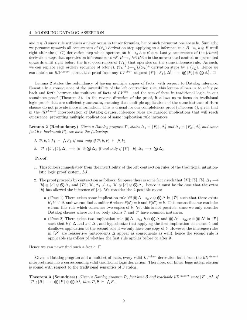
Lemma 2 states the redundancy of having multiple copies of facts, with respect to Datalog inference.Essentially a consequence of the invertibility of the left contraction rule, this lemma allows us to safely goback and forth between the multisets of facts of LV obs− and the sets of facts in traditional logic, in oursoundness proof (Theorem 3). In the reverse direction of the proof, it allows us to focus on traditionallogic proofs that are sufficiently saturated, meaning that multiple applications of the same instance of Hornclauses do not provide more information. This is crucial for our completeness proof (Theorem 4), given thatin the llDAssert interpretation of Datalog clauses, inference rules are guarded implications that will reachquiescence, preventing multiple applications of same implication rule instances.

Lemma 2 (Redundancy) Given a Datalog program P, states ∆1 ≡ dF1e,∆]1 and ∆2 ≡ dF2e,∆]

2 and somefact b ∈ herbrand(P), we have the following:

1. P, b, b, F1 `∧F2 if and only if P, b, F1 `

∧F2

2. dPe; dbe, dbe,∆1 −→ dbe ⊗⊗

∆2 if and only if dPe; dbe,∆1 −→⊗

∆2

Proof:

1. This follows immediately from the invertibility of the left contraction rules of the traditional intuition-istic logic proof system, LJ .

2. The proof proceeds by contraction as follows: Suppose there is some fact c such that dPe; dbe, dbe,∆1 −→dbe ⊗ dce ⊗

⊗∆2 and dPe; dbe,∆1 6−→Σ dbe ⊗ dce ⊗

⊗∆2, hence it must be the case that the extra

dbe has allowed the inference of dce. We consider the 2 possible cases:

• (Case 1) There exists some implication rule ∀~x⊗

∆ (a c ⊗⊗

∆ in dPe such that there existsb′, b′′ ∈ ∆ and we can find a unifier θ where θ(b′) = b and θ(b′′) = b. This means that we can inferc from this rule which consumes two copies of b. Yet this is not possible, since we only considerDatalog clauses where no two body atoms b′ and b′′ have common instances.

• (Case 2) There exists two implication rule⊗

∆(a1 h⊗⊗

∆ and⊗

∆′ (a2 c⊗⊗

∆′ in dPesuch that b ∈ ∆ and b ∈ ∆′, and hypothesize that applying the first implication consumes b anddisallows application of the second rule if we only have one copy of b. However the inference rulesin dPe are reassertive (antecedents ∆ appear as consequents as well), hence the second rule isapplicable regardless of whether the first rule applies before or after it.

Hence we can never find such a fact c. �

Given a Datalog program and a multiset of facts, every valid LV obs− derivation built from the llDAssert

interpretation has a corresponding valid traditional logic derivation. Therefore, our linear logic interpretationis sound with respect to the traditional semantics of Datalog.

Theorem 3 (Soundness) Given a Datalog program P, fact base B and reachable llDAssert state dF e,∆], ifdPe; dBe −→

⊗dF e ⊗

⊗∆], then P,B `

∧F .

9


Proof: For any sequent dPe; dBe −→⊗dF e ⊗

⊗∆] constructed from our Datalog interpretation,

we inductively define their corresponding normalized derivations as follows: the rule (obs) is the only basestructural rule, while (IL) is the only inductive structural rule. By the form of the (IL) rule, we can concludethat all intermediate sequents of the derivation are of the form dPe; dF ′e,∆′] −→

⊗dF e⊗

⊗∆], with initial

sequents as a special case, such that dF ′e ≡ dBe and d∆′e ≡ ∅. By Lemma 1, we can safely assert that nosequents other than those generated by the base (obs) and inductive (IL) structural rules are valid derivationsof our Datalog interpretation. The inductive proof proceeds as follows:

• Base (obs) structural rule: We consider the sequent proof built from the (obs) derivation rule ofLV obs−. Hence for dPe; dF ′e,∆′] −→

⊗dF e ⊗

⊗∆] to be derivable for the (obs) rule, we must have

dF ′e ≡ dF e and ∆′] ≡ ∆]. As such we need to show that P, F ′ `∧F . This is proven in sequent

calculus LJ simply by applications of the left weakening rule (WL) to discard P from the left, separating∧F with applications of the right ∧ rule (∧R) and finishing up with applications of the identity rule

(id).

• Inductive (IL) structural rule: We consider a macro derivation step (IL). Induction hypothesis, weassume that for dPe ≡ Γ, (∀~x.

⊗B(a h⊗

⊗B), we have dPe; [~t/~x]h, [~t/~x]B,B′,∆′], [~t/~x]a−→

⊗dF e⊗⊗

∆] where dF ′e ≡ [~t/~x]h, [~t/~x]B,B′ and also P, F ′ ` F . By applying the (IL) rule, we havedPe; [~t/~x]B,B′,∆′] −→

⊗dF e ⊗

⊗∆]. We now need to prove that we also have P, F ′′ `

∧F such

that [~t/~x]h, F ′′ ≡ F ′. We do this by considering a sequence of LJ derivations that mimics the (IL) rule,specifically we do the following: we apply left contraction (CL) rules on each [~t/~x]B ∈ F ′ then we applythe Datalog rule D = ∀~x. B ⊃ h such that dDe ≡ ∀~x.

⊗B(a h⊗

⊗B to obtain P, [~t/~x]h, F ′′ ` F

as the premise, which happens to be assumed valid by our induction hypothesis P, F ′ ` F (since[~t/~x]h, F ′′ ≡ F ′).

Hence we have shown that Theorem 3 holds for all normalized derivations. �

Given a Datalog program and a set of facts, every valid traditional logic derivation built from thetraditional Horn clause interpretation of Datalog, has a corresponding LV obs− derivation built from itsllDAssert interpretation. Our interpretation is therefore also complete.

Theorem 4 (Completeness) Given a Datalog program P, fact base B and F ⊆ herbrand(P), if P,B `∧F ,

then there is ∆ such that dPe; dBe −→⊗dF e ⊗

⊗∆.

Proof: The proof of this theorem is similar to the proof of Theorem 3, except that we do structuralinduction on derivations of the corresponding fragment of LJ proof system (Figure 3), over well-formedDatalog programs and facts. We inductively define the LJ derivations we consider as follows: Base structuralderivation steps built from left weakening (WL) rules, (id) rules and right conjunction (∧R) rules, whileinduction structural steps consist of an orderly sequence of derivation steps that correspond to application ofHorn clauses. Specifically for a Datalog clause ∀~x. B ⊃ h, we instantiate the Horn clause by applying (∀L)rule on each variable ~x, then left contraction rules (CL) on each atomic formula in the context that matchesto B, apply the implication rule (⊃L). We rely on permutability results of LJ derivations [MNPS91] to safelyrestrict our attention to only sequents inductively generated by the above. Since we define our inductivesteps in this manner, all intermediate sequents during the inductive steps are of the form P, F ′ `

∧F

where B ⊆ F ′, with the initial sequent being a special case such that F ′ ≡ B. We also exploit the resultsfrom Lemma 2 that states that multiple copies of facts are redundant, allowing us to omit LJ derivationsthat contains multiple applications of same Horn clause instances that produces the same facts (we cannotreplicate this in LV obs− guarded implications). The inductive proof proceeds as follows:

• Base structural rule: We consider the LJ sequent proof built from left weakening (WL) rules, (id)rules and right conjunction (∧R) rules. Hence for P, F ′ `

∧F to apply, we must have F ′ ≡ F . As

such, from P, F ′ `∧F we can use (WL) rules to remove P from the context, (∧R) rules to break

apart∧F and (id) rules to match the individual atomic formulas in F . We need to show for some ∆]

10


and ∆ that dPe; dF ′e,∆] −→⊗dF e ⊗∆. Since F ′ ≡ F , we have ∆] ≡ ∆ and apply the (obs) rule.

• Inductive structural rule: We consider the sequence of LJ derivation rules which involves theorderly sequence of derivation steps that results to the applications of Horn clauses as defined above.Induction hypothesis, we assume that given P, [~t/~x]h, [~t/~x]B,B′ `

∧F and P ≡ Γ, (r : ∀~x. B ⊃ h) for

some Γ, then we have dPe; [~t, ~x]dhe, [~t/~x]dBe, dB′e,∆] −→⊗dF e ⊗∆ for some ∆] and ∆. We show

that we have the LJ sequent P, [~t/~x]B,B′ `∧F through the following LJ derivation steps: from

P, [~t/~x]B,B′ `∧F , given the Datalog clause r : ∀~x. B ⊃ h we apply (∀L) derivation steps on each

variable in ~x, followed by (CL) rules on each [~t/~x]B in the context. Next, we apply this implicationrule to obtain P, [~t/~x]h, [~t/~x]B,B′ `

∧F as the premise of our derivation, which we assumed in our

induction hypothesis. We now show that dPe; [~t/~x]dBe, dB′e,∆′′] −→⊗dF e⊗∆ has a valid derivation

for some ∆′′]. We do this by applying the (IL) derivation step of the corresponding inference rule, i.e.,∀~x. B(r(~x) h⊗B, which yields dPe; [~t, ~x]dhe, [~t/~x]dBe, dB′e,∆′′], r(~t) −→

⊗dF e⊗∆ as the premise,

and by having ∆] ≡ ∆′′], r(~t) we have our induction hypothesis. Hence we proved the inductive case.

Hence we have shown that Theorem 4 holds for all normalized derivations. �

From Theorems 4 and 3, we have that the soundness and completeness. Given a fact base B, we canalways derive a state dF e, d∆]e such that the set interpretation of dF e (denoted set(F )) is equal to P(B)and this state is quiescent. Further more, there can only be one such quiescent state.

Theorem 5 (Correctness) Let P be a Datalog program and B a collection of base facts.

1. There are dF e and ∆] such that dPe; dBe −→⊗dF e ⊗

⊗∆] and Quiescent(dPe, (dF e,∆])) and

set(F ) = P(B).

2. For any state ∆, if dPe; dBe −→⊗d∆e and Quiescent(dPe,∆), then there is ∆] such that ∆ = dF e,∆]

and set(F ) = P(B).

Proof: We prove (1) and (2) as follows:

1. From Theorem 4, we can conclude that since P,B `∧P(B), then we have dPe; dBe −→

⊗dF e⊗

⊗∆]

for some ∆] and set(F ) = P(B). We prove that Quiescent(dPe, (dF e,∆])) by contradiction: Sup-pose that Quiescent(dPe, (dF e,∆])) does not hold, hence we can apply more derivation rules fromthat state. Yet given that our Datalog interpretation only has inference rule instances of the form⊗B (a h ⊗

⊗B which are reassertive, applying more such rules only produces an inferred fact h

such that h /∈ P(B). Yet we have a corresponding Datalog clause instance B ⊃ h that should have beenapplied and captured in the inferential closure P(B) (i.e. h ∈ P(B)), as such we have a contradiction.Hence, we must have Quiescent(dPe, (dF e,∆])).

2. Suppose that we have dPe; dBe −→⊗d∆e and Quiescent(dPe,∆), but there is no ∆] such that ∆ =

dF e,∆] and set(F ) = P(B). The implies that either we have set(F ) ⊂ P(B) or set(F ) ⊃ P(B). We can-not have set(F ) ⊃ P(B) since by Theorem 3, we cannot infer more facts than P(B) (i.e. P,B `

∧F ),

but yet we cannot have set(F ) ⊂ P(B) either, which would contradict Quiescent(dPe,∆). Hence ourassumption that there is no ∆] such that ∆ = dF e,∆] and set(F ) = P(B) has reached a contradiction.

Hence we have shown that Theorem 5 holds �

These results are incremental steps towards achieving the main goal of this report, which is to formalizean interpretation of both assertion and retraction in Datalog, done in Section 5.

11

5 MODELING DATALOG RETRACTION

P = I : ∀x. A(x) ∧B(x) ⊃ D(x) VPW = ∀x. I(x)1

I(x)1 = A(x)⊗B(x)(I](x) D(x)⊗A(x)⊗B(x)⊗R(x)

1 ⊗ A](x)⊗B](x)

R(x)1 = (A(x)⊗ A](x)⊗B](x) ( D(x)⊗ A(x)) & (B(x)⊗ A](x)⊗B](x) ( D(x)⊗ B(x))

AP = ∀x. A(x)A ,∀x. A(x)

B ,∀x. A(x)D

A(x)A = A(x)⊗ A(x) (A](x) (A](x)( 1)

A(x)B = B(x)⊗ B(x) (B](x) (B](x)( 1)

A(x)D = D(x)⊗ D(x) (D](x) (D](x)( 1)

Assertion of B(5): *A(5)++B(5)

====⇒LL

VPW ∆′ where ∆′ = *A(5), B(5), D(5),R(5)1 , I](5), A](5), B](5)+

(obs)

VPW,AP ; A(5), B(5), D(5),R(5)1 , I](5), A](5), B](5) −→

⊗∆′

I(5)1

VPW ,AP ; A(5), B(5) −→⊗

∆′

Retraction of A(5): ∆′−A(5)

====⇒LL

VPW ∆′′ where ∆′′ = *B(5)+

(obs)VPW,AP ; B(5) −→

⊗∆′′

A(5)A

VPW, AP ; A(5) , B(5), A(5) −→⊗

∆′′

A(5)D

VPW, AP ;A(5), B(5), D(5) , A(5), D(5) −→⊗

∆′′

R(5)1

VPW,AP ;A(5), B(5), D(5), R(5)1 , I](5), A(5), A](5), B](5) −→

⊗∆′′

Figure 10: An Example of llDFull Interpretation

5 Modeling Datalog Retraction

In this section, we extend our linear logic interpretation of Datalog assertion to also account for the retractionof facts. We first illustrate our technique in Section 5.1 by informally introducing a simplified versioncalled llDFull−. Unfortunately, this simplified version admits LV obs− sequent derivations that correspond toincomplete retraction of facts, meaning that when such a derivation reaches quiescence there is no guaranteethat the state we obtain corresponds to a valid Datalog object. In Section, 5.2, we modify it into the llDFull

interpretation that provides guarantees of completeness when quiescence is achieved. Then in Section 5.3, weformally define the llDFull interpretation that incorporates this modification and correctly models Datalogassertion and retraction.

5.1 Retraction and Absorption Rules

We model the removal of facts by means of anti-predicates. An anti-predicate p is an ordinary predicatethat is meant to be equal and opposite to p. While p applied to terms ~t forms a fact, p applied to termsform a retraction fact. For instance, recalling the reachability example from Figure 5, the predicates E andP will have equal and opposite anti-predicates E and P respectively. The intent is that an atom p(~t) willultimately absorb its equal and opposite atom p(~t). To model this property, we define absorption rules of

12


Fact Vp(~t)W = p(~t)

Program

{VD, PW = VDW,VPWV.W = .

Conjunction Vb ∧BW = VbW⊗ VBW

Clause Vr : ∀~x. B ⊃ hW = ∀~x. VBW(r](~x) VhW⊗ VBW⊗ VB]W⊗Ret(B,B, r](~x), h)

Fact base

{VB, aW = VBW,VaWV∅W = .

where

Ret(b ∧B′, B, r](~x), h) = (VbW⊗ r](~x)⊗ VB]W( VhW⊗ VbW) & Ret(B′, B, r](~x), h)

Ret(b, B, r](~x), h) = (VbW⊗ r](~x)⊗ VB]W( VhW⊗ VbW)

Figure 11: llDFull Interpretation of Datalog

the form ∀~x. p(~x) ⊗ p(~x) ( 1. We illustrate this by means of an example, displayed in Figure 9, which

shows a Datalog program P and its llDFull− interpretation. We have three absorption rules A(x)− , one for

each predicate of this Datalog program. Also demonstrated here, we enrich the linear logic interpretation ofDatalog programs with retraction rules: Each Datalog clause r : ∀~x. p1(~t1)∧ . . .∧pn(~tn) ⊃ ph(~th) is modeledby a inference rule that contains an additional consequent, the additive conjunction of n retraction rules,

each of which is uniquely associated with one of the antecedents pi(~ti). For instance, inference rule I(x)1 has

an embedded retraction rule R(x)1 in its consequent and R(x)

1 contains two linear implications, joined by the& operator. Each of these linear implications produces a retraction of D(x) (i.e., D(x)) in the event that wehave a retraction of B(x) or C(x) respectively.

In the llDFull− interpretation of Datalog programs, we can always find a valid LV obs− derivation thatrepresents each assertion or retraction of facts. Figure 9 illustrates two such derivations, starting from astate containing just the fact A(5), the first derivation shows a derivation in the llDFull− interpretation ofthis program, that models the assertion of a new fact B(5). As such, we consider the derivation startingfrom the initial state, consisting of A(5) and the newly asserted fact B(5). We highlight (using boxes) theactive fragments of the sequent which contributes to the application of the derivation step. Notice that when

the inference rule instance I(5)1 applies, we have not only the inferred fact D(5), but we have the retraction

rule instance R(5)1 as well. This retraction rule is bookkeeping information that will facilitate the retraction

of D(5), in the event that either A(5) or B(5) is retracted. To illustrate this, the second derivation of thisfigure models the retraction of fact A(5). We consider the state ∆′ (obtained in the previous derivation)with the retraction atom A(5) inserted. A(5) and I](5) triggers the first additive conjunction component

A(5)⊗I](5)( D(5)⊗A(5) of the retraction rule instance R(5)1 and produces D(5) while retaining A(5). The

purpose of retaining A(5) is that in the general case, A(5) might be necessary for triggering the retraction ofother atoms, yet we consume I](5) to allow future applications of inference rule instance I](5) should A(5)

be re-asserted by future updates. Joining the linear implications of retraction rule R(x)2 with the & operator

allows the creation of exactly one D(5) atom from the retraction of B(5) or C(5). Hence we will not be left

with a “dangling” copy of D(5) should C(5) be retracted as well (since R(5)1 has completely been consumed

by B(5)). We finally complete the derivation by applying the absorption of D(5) and A(5) by D(5) and

A(5), via absorption rules A(5)D and A(5)

A respectively. Note that ∆ and ∆′ are quiescent with respect to thellDFull− interpretation of the Datalog program.

13


5.2 Quiescence and Complete Retraction

In this section we address a shortcoming of the llDFull− interpretation: we cannot guarantee that reachablestates derived by valid LV obs− derivations model complete retraction of Datalog facts when they reachquiescence.

Refer to Figure 9 again. In the second derivation, which corresponds to the retraction of A(5) starting

from state ∆′, A(5), rather than applying retraction rule R(5)1 , we could have instead immediately applied

the absorption rule instance A(5)1 , yielding a state of quiescence and bypassing the retraction of D(5). This

state, however, would be an incorrect representation of the effect of retracting A(5), hence such derivationsshould somehow be disallowed. In general, any pair of equal and opposite atoms p(~t) and p(~t) should beapplied to (and consumed by) their corresponding absorption rule only when all retraction rules that can beapplied to p(~t) have been applied. In other words, we must inhibit the application of absorption rules untilall such retraction rules have been applied. To do so, we use the same technique with which we achievedquiescence in the presence of reassertive inference rules: guarded linear implications. Specifically we requirethat for each inference rule that is applied, for each antecedent p(~t) of this inference rule we produce a witnessatom p](~t); retraction rules additionally consume these witness p](~t). We define absorption rules as guardedimplications p(~x) ⊗ p(~x) (p](~x) (p](~x) ( 1). The witnesses inhibit absorption rules until they are finally

removed by retraction rules. Notice that an absorption rule produces a peculiar consequent p](~x)( 1. Thepurpose for this is to consume the atom p](~x) produced as a consequent of applying the ((−L ) rule.

Figure 10 illustrates this idea on our last example. The boxes highlight the components added on top ofthe llDFull− interpretation example of Figure 9. We call it the llDFull interpretation, implemented by the

function V−W, defined in Section 5.3. Specifically inference rule I(x)1 has two additional consequents A](x)

and B](x), which are witness atoms for antecedents A(x) and B(x) respectively. Absorption rules are now

guarded linear implications with witness atoms as inhibitors. For instance, A(x)A can only apply if there

are no witnesses A](x) in the context. Finally, on top of consuming inference witness I](x) and producing

retraction atom D(x), the retraction rules in R(x)1 have the additional responsibility of consuming witness

atoms A](x) and B](x).

Figure 10 shows derivations for the llDFull interpretation of our last example (Figure 9). The firstderivation corresponds to the assertion of B(5) starting from a state containing a single A(5) and is similarto that in Figure 9 except we additionally infer witness atoms A](5) and B](5). The next derivation illustrates

the subsequent retraction of A(5). Now absorption rule A(5)A cannot be applied to A(5) and A(5) as there is a

witness atom A](5) inhibiting A(5)A . The only possible way forward is the application of retraction rule R(5)

1 ,

which on top of producing retraction atom ˜D(5) and consuming inference witness I](5), consumes witness

atoms A](5) and B](5), thereby unlocking the applicability of A(5)A .

5.3 The llDFull Interpretation

We now formalize the llDFull interpretation of Datalog programs. For each atom representing a fact p(~t), wedefine its equal and opposite retraction atom p(~t). We will extend this notation to collections of atoms, hencefor a multiset of atoms ∆, we denote a multiset of all equal and opposite retraction atoms of ∆ is denoted∆. Beside the rule witnesses r](~x) of Section 4.1, for each atom p(~x) we have another type of witnesses, thefact witness p](~x). While a rule witness r](~t) witnesses the application of an inference rule instance of r, afact p(~t) witnesses a use of p](~t) to infer some other fact. Given a Datalog program P, for each predicate pof some arity n, we define the set of all absorption rules AP as follows:

AP = *∀~x.p(~x)⊗ p(~x)(p](~x) (p](~x)( 1) | p in P+

Figure 11 formalizes the llDFull interpretation of Datalog programs as the function V−W. The maindifference between this function and the function d−e of llDFull− is that Datalog clauses are inferencerules that include two additional types of consequents. Specifically, a retraction rule which is an additive

14


Let VPW ≡ Γ, II ≡ ∀~x.

⊗∆(r](~x) h⊗

⊗∆⊗Rr ⊗

⊗∆]

r](~t) /∈ ∆′

VPW,AP ; [~t/~x](h,∆,Rr,∆]), r](~t),∆′ −→ C(IL)

VPW,AP ; [~t/~x]∆,∆′ −→ C


r](~t) /∈ ∆′

VPW,AP ; [~t/~x](h,∆,Rr), r](~t), [~t/~x]∆],∆′ −→ C(⊗L)*

VPW,AP ; [~t/~x](h⊗⊗

∆⊗Rr ⊗⊗

∆]), r](~t),∆′ −→ C((−L )

VPW,AP ; [~t/~x]I , [~t/~x]∆,∆′ −→ C(∀L)*

VPW,AP ; I , [~t/~x]∆,∆′ −→ C(clone)

VPW,AP ; [~t/~x]∆,∆′ −→ C

Figure 12: llDFull Inference Macro Rule

conjunction of linear implications defined by the function Ret and a tensor closure of inference fact witnessesderived from the antecedents of the inference rule. Altogether, given a Datalog clause r : ∀~x. B ⊃ h, itscorresponding inference rule in llDFull interpretation infers three types of bookkeeping information, namely,the retraction rule Rr, the rule witness r](~x) and fact witnesses B].

Given a Datalog program P, a multiset of facts F ⊆ herbrand(P) and a multiset of retraction rules∆R and a multiset of witness atoms ∆], a llDFull state of this Datalog program is an LV obs− linear con-text VFW,∆R,∆]. Given base facts B ⊆ herbrandB(P), the state dF e,∆R,∆] is reachable from B ifVPW; dBe −→

⊗VFW⊗

⊗∆R⊗

⊗∆] is derivable. Note that VBW is always reachable from B — it is called

an initial state.

Similarly to Figure 8, Figure 12 defines the inference macro derivation rule for the llDFull interpretation.

Figure 14 introduces the retraction macro step, which models the retraction of some fact h. As definedin Figure 11 by the function Ret, a retraction rule Rr is an additive conjunction of linear implications ofthe form ai ⊗ r(~t) ⊗

⊗∆] ( ai ⊗ h, which are reassertive (antecedent ai appears as consequent) and the

only component that varies among the linear implications is the antecedent ai. As such, retraction rule Rrcan be viewed as a formula that reacts to any ai which is an antecedent of one of its linear implications and,when applied, consumes rule witness r(~t) and fact witnesses ∆], and produces h.

Figure 15 defines the last of the three macro derivation steps of the llDFull interpretation. It models theabsorption of an atom p(~t) and the equal and opposite p(~t), but only in the absence of any witness p](~t).

Figure 13 illustrates the top-level formulation of the main goal of this report, defining ==⇒LL

VPW, our linear

logic specification of Datalog assertion and retraction in terms of LV obs− derivations. In contrast to thelogical specification ==⇒P in Figure 1 which defines assertion and retraction based on inferential closuresof base facts, ==⇒LL

VPW is defined as follows: the assertion of a new base fact a to a state ∆ maps to the

derivation with fact a inserted into the original state, while the retraction an existing base fact a from state∆ maps to a derivation with a inserted. In both cases, we consider only resulting states which are quiescent.Theorem 13 in Section 5.5 states the correspondence of the llDFull interpretation that formally prove thecorrectness this logical specification.

5.4 Cycles and Re-assertion

In this section, we analyze two aspects of the llDFull interpretation. Specifically, we discuss cycles in Dataloginference and the need for re-assertion when doing retraction.

15


a /∈ ∆ VPW,AP ; ∆, a −→⊗

∆′ Quiescent(∆′, (VPW,AP))

∆+a

==⇒LL

VPW ∆′(Infer)

a ∈ ∆ VPW,AP ; ∆, a −→⊗

∆′ Quiescent(∆′, (VPW,AP))

∆−a

==⇒LL

VPW ∆′(Retract)

Figure 13: Assertion and Retraction, in llDFull

Quiescence in Cycles: One important issue to consider for the llDFull interpretation, is whetherquiescence can be achieved for Datalog programs with cycle. Figure 16 shows one such example modifiedfrom the graph example of Figure 6, along with its linear logic interpretation (we omit the absorption rulesfor brevity). This example attempts to generate reflexive paths P (x, y) from base facts E(x, y) that representedges. Figure 16 also illustrates an LV obs− derivation which represents the assertion of E(4, 5) which in fact,

achieves quiescence: We infer the facts P (4, 5) and P (5, 4) through inference rule instances I(4,5)1 and I(4,5)

2 ,

as well as an additional copy of P (4, 5) through I(5,4)2 , before we reach quiescence. We omit fact witnesses

and retraction rules as they are inessential in this discussion. In general, as long as Datalog clauses arewell-formed and the set Σ of all possible constants is finite, the llDFull interpretation of Datalog programswill reach quiescence under LV obs− derivations. This is because the possible combinations of rule instancesare finite, and since for each rule instance we can apply it at most once in a derivation, all LV obs− derivationsof well-formed Datalog programs reach quiescence.

Re-assertion during Retraction: In some cases, re-assertion of facts occurs during retraction whileworking towards quiescence. Figure 17 illustrates a Datalog program which exhibits such a behavior. Fromeither base facts A(x) or B(x), we can infer C(x). We consider an initial state ∆ where A(2) and B(2) has

been asserted. Hence, inference rule instances I(2)1 , I(2)

2 and I(2)3 has been applied before reaching quiescence

at state ∆. Note that while we have two copies of C(2) (from I(2)1 and I(2)

2 ), we only have one copy of D(2),

since rule instance I(2)3 is only permitted to be applied once. Next we consider the situation when A(2) is

retracted, triggering the application of retraction rules R(2)1 and R(2)

3 which ultimately absorbs A(2), C(2)and D(2). This leads us to a seemingly inconsistent state, where B(2) and C(2) exists, yet D(2) has beencompletely retracted as part of the retraction closure of A(2). However, quiescence is only achieved when

inference rule instance I(2)3 is re-applied, re-asserting another copy of D(2). While re-assertion guarantees

the re-completion of assertion closures of the llDFull interpretation, it arguably adds overheads. One of ourfuture objectives is to refine the llDFull interpretation to overcome the need for re-assertion during retraction.

5.5 Correctness

In this section, we highlight the proofs of correspondence of the llDFull linear logic interpretation of Datalogprogram.

For any LV obs− sequents constructed from the llDFull interpretations of Datalog assertion, we can alwaysfind a normalized LV obs− derivation that consists only of (IL) and (obs) derivation rules. Similarly, forsequents from llDFull interpretations of Datalog retraction, we can find normalized derivations that consiststrictly only of (IL), (RL), (AL) and (obs) derivation rules. This will simplify the proof of the correctnessof our interpretation.

Lemma 6 (Normalized Derivations) Given Datalog program P, llDFull states VF1W,∆R1 ,∆]1 and

VF2W,∆R2 ,∆]2, a LV obs− derivation VPW,AP ; VF1W,∆R1 ,∆

]1 −→

⊗VF1W⊗

⊗∆R2 ⊗

⊗∆]

2 has a proof con-sisting of only applications of (IL), (RL), (AL) and (obs) derivation rules.

Proof: The bulk of the proof of this Lemma is derived from permutability results of linear logic [GPI94].

16


Let Ri ≡ ai ⊗ r(~t)⊗⊗

∆]( ai ⊗ h

VPW,AP ; ak, h,∆ −→ C(RL)

VPW,AP ; ak,&ni=1Ri, r(~t),∆],∆ −→ C

for some k ≥ 1 and k ≤ n, which decomposes into:

VPW,AP ; ak, h,∆ −→ C(⊗L)

VPW,AP ; ak ⊗ h,∆ −→ C((L)

VPW,AP ; ak,Rk, r(~t),∆],∆ −→ C(&L)*

VPW,AP ; ak,&ni=1Ri, r(~t),∆],∆ −→ C

Figure 14: llDFull Retraction Macro Rule

Essentially, we need to disentangle a generic derivation of any sequent VPW,AP ; VF1W,∆R1 ,∆]1 −→

⊗VF1W⊗⊗

∆R2 ⊗⊗

∆]2, into one which comprises of an orderly sequence of LV obs− derivation steps that correspond to

macro derivation steps (IL), (RL) and (AL) of Figure 12, 14 and 15, and ending off with a (obs) derivationstep. We do this by showing that thanks to permutability results in [GPI94], we can safely rearrangederivation steps. Most of the proof is very similar to Lemma 1, except that derivation steps may have tobe pushed pass the problematic (&) rule. Thankfully, retraction rules (the only formula where & operatorappears in) are designed to be confluent: regardless of which & sub-formula is chosen, the same effect isachieved, for instance retraction rule &n

i=1(ai ⊗ r(~t) ⊗∆] ( ai ⊗ h) ultimately removes witnesses r(~t) and∆], and introduces h regardless of which sub-formula is chosen. As such, all other derivation steps can besafely pushed pass it. We list the details of these permutation operation for each macro rule:

• (IL) rule: The proof is similar to Lemma 1, since the inference rule of llDFull interpretation (Figure 12)is of the same form as llDAssert inference rules (Figure 8), only the body contains additional witnessatoms and retraction rules, which involves additional applications of (⊗L) and does not affect theresults of Lemma 1.

• (RL) rule: For a retraction rule &ni=1(ai ⊗ r(~t) ⊗ ∆] ( ai ⊗ h), since the top most (⊗L) rule that

operates on the body of the retraction implication rule ak ⊗ h can be pushed downwards until rightbefore the ((L) derivation step that applied on the retraction implication rule. Next, we have to pushall (&L) rules applied on the retraction rule upwards to the rule application ((L) derivation step.This is possible because of the confluence result in retraction rules stated above.

• (AL) rule: We can push the top most (1L) and ((L) derivation steps to just right after the ((−L )derivation step of an application of the (AL) macro rule. Similarly to the (IL) macro rule, (clone) and(∀L) derivation steps can be safely pushed upwards until right before the main ((−L ) derivation step.

Hence we have shown that all LV obs− derivations has a proof consisting of only the rules (IL), (RL), (AL)and (obs). �

For every llDFull derivation that models the assertion of facts (excluding retraction), we have a corre-sponding llDAssert derivation and vice versa. Both directions depend on the fact that witness facts andretraction rules have no effects on the assertion of new facts.

Lemma 7 (Completeness and Soundness of Assertion) Given a Datalog Program P, for any fact base

B, multiset of facts F ⊆ herbrand(P), multiset of rule witnesses ∆]R, multiset of fact witnesses ∆]

F and

17


Let ∀~x. p(~x)⊗ p(~x)(p](~x) (p](~x)( 1) ∈ AP

p](~t) /∈ ∆ VPW,AP ; ∆ −→ C(AL)

VPW,AP ; p(~t), p(~t),∆ −→ C


p](~t) /∈ ∆

VPW,AP ; ∆ −→ C(1L)

VPW,AP ; 1,∆ −→ C((L)

VPW,AP ; (p](~t)( 1), p](~t),∆ −→ C((−L )

VPW,AP ; (p(~t)⊗ p(~t)(p](~t) (p](~t)( 1)), p(~t), p(~t),∆ −→ C(∀L)*

VPW,AP ;Ap, p(~t), p(~t),∆ −→ C(clone)

VPW,AP ; p(~t), p(~t),∆ −→ C

Figure 15: llDFull Absorption Macro Rule

multiset of retraction rules ∆R,

VPW,AP ; VBW −→⊗

VFW⊗⊗

∆R ⊗⊗

∆]R ⊗

⊗∆]F if and only if dPe; dBe −→

⊗dF e ⊗

⊗∆]R

Proof:

• (⇒) For any llDFull derivation, we safely omit witnesses and retraction rules to obtain a llDAssert

derivation. This is because inference rules in both interpretations are the same, except that llDFull

inference rules have additional witnesses and retraction rules as consequents, which do not derive newfacts.

• (⇐) We show that any llDAssert normalized derivation has a corresponding llDFull normalized deriva-

tion, i.e. in general, if dPe; dF1e,∆]R1 −→

⊗dF2e ⊗

⊗∆]R2 then VPW,AP ; VF1W,∆R1 ,∆

]F1,∆

]R1 −→⊗

VF2W ⊗⊗

∆R2 ⊗⊗

∆]F2 ⊗

⊗∆]R2 for some ∆R1 , ∆R2 , ∆]

F1 and ∆]F2. We inductively define the

llDAssert derivation as follows: Base structural derivations steps are built from (obs) rule, while in-ductive structural derivation steps are built from (IL) macro rule of the llDAssert interpretation. Theinductive proof proceeds as follows:

– Base structural rule: We consider the application of the (obs) rule. Hence for

dPe; dF1e,∆]R1 −→

⊗dF2e⊗

⊗∆]R2 to result from the (obs) rule, we must have dF1e ≡ dF2e and

d∆R1e ≡ d∆R2e. We show that there exist some ∆R1 , ∆R2 , ∆]F1 and ∆]

F2 such that the llDFull

sequent VPW,AP ; VF1W,∆R1 ,∆]F1,∆

]R1 −→

⊗VF2W⊗

⊗∆R2 ⊗

⊗∆]F2⊗

⊗∆]R2 has a derivation

as well. For that we simply choose ∆R1 ≡ ∆R2 and ∆]F1 ≡ ∆]

F2, hence the llDFull sequent inquestion applies to the (obs) rule as well.

– Inductive structural rule: We consider the application of the llDAssert (IL) macro derivation

step. Induction hypothesis, we assume that if we have dPe; [~t/~x]dhe, [~t/~x]dBe, dB′e,∆]R, r(~t) −→⊗

dF2e ⊗⊗

∆]R2 such that (∀~x.

⊗B (r(~x) h ⊗

⊗B) ∈ dPe, then for some ∆R1 , ∆R2 , ∆]

F1

and ∆]F2, we have VPW,AP ; [~t/~x]VhW, [~t/~x]VBW,VB′W,∆R1 ,∆

]R1,∆

]F1, r(~t) −→

⊗VF2W⊗

⊗∆R2 ⊗⊗

∆]R2⊗

⊗∆]F2. For the llDAssert sequent, we apply a llDAssert (IL) macro derivation step to ob-

taindPe; [~t/~x]dBe, dB′e,∆]

R −→⊗dF2e ⊗

⊗∆]R2. We now need to show that

VPW,AP ; [~t/~x]VBW,VB′W,∆R3 ,∆]R1,∆

]F3 −→

⊗VF2W⊗

⊗∆R4 ⊗

⊗∆]R2 ⊗

⊗∆]F4 for some ∆R3 ,

18


P = I1 : ∀x, y. E(x, y) ⊃ P (x, y) , I2 : ∀x, y. P (x, y) ⊃ P (y, x)

VPW = ∀x, y. I(x,y)1 , ∀x, y. I(x,y)

2

I(x,y)1 = E(x, y)(I]1(x,y) P (x, y)⊗ E(x, y)⊗ E](x, y)⊗R(x,y)

1

R(x,y)1 = E(x, y)⊗ I]1(x, y)⊗ E](x, y)( P (x, y)⊗ E(x, y)

I(x,y)2 = P (x, y)(I]2(x,y) P (y, x)⊗ P (x, y)⊗ P ](x, y)⊗R(x,y)

2

R(x,y)2 = P (x, y)⊗ I]2(x, y)⊗ P ](x, y)( P (y, x)⊗ P (x, y)

Assertion of E(4, 5): ∅ +E(4,5)=====⇒P ∆ where ∆ = *P (4, 5), P (5, 4), P (4, 5), E(4, 5), I]1(4, 5), I]2(4, 5), I]2(5, 4), ..+

(obs)VPW,AP ; P (4, 5), P (5, 4), P (4, 5), E(4, 5), I]1(4, 5), I]2(4, 5), I]2(5, 4), .. −→

⊗∆

I(5,4)2

(IL)VPW ,AP ; P (5, 4) , P (4, 5), E(4, 5), I]1(4, 5), I]2(4, 5), .. −→

⊗∆

I(4,5)2

(IL)VPW ,AP ; P (4, 5) , E(4, 5), I]1(4, 5), .. −→

⊗∆

I(4,5)1

(IL)VPW ,AP ; E(4, 5) −→

⊗∆

Figure 16: Example of Quiescence in the Presence of Cycles

∆R4 , ∆]F3 and ∆]

F4. To do this, we apply the llDFull (IL) macro derivation step corresponding tothe llDFull inference rule instance (∀~x.

⊗B (r(~x) h ⊗

⊗B ⊗

⊗∆] ⊗R) ∈ VPW. We obtain a

derivation step with premise VPW,AP ; [~t/~x]VhW, [~t/~x]VBW,VB′W, [~t/~x],R,∆R3 , r(~t),∆]R3, [~t/~x]∆],∆]

F3

−→⊗

VF2W ⊗⊗

∆R4 ⊗⊗

∆]R2 ⊗

⊗∆]F4 where if we take ∆R1 ≡ R,∆R3 , ∆]

F1 ≡ [~t/~x]∆],∆]F3,

∆R2 ≡ ∆R4 and ∆]F2 ≡ ∆]

F4, is exactly equivalent to our induction hypothesis.

Hence we have proven the completeness and soundness of assertions. �

We show that for derivations that do not consist of anti-predicates (retraction of facts), we have aquiescent state in llDFull corresponds to a quiescent state in llDAssert .

Lemma 8 (Correspondence of Quiescence) Let P be a Datalog program and B a collection of base facts,for any F,∆R,∆] such that VPW,AP ; VBW −→

⊗VFW⊗

⊗∆R ⊗

⊗∆],

Quiescent((VPW,AP), (VFW,∆R,∆])) if and only if Quiescent(dPe, (dF e,∆]))

Proof: This follows from Lemma 7. We show by contradiction:

• (⇒) Suppose that Quiescent((VPW,AP), (VFW,∆R,∆])) but Quiescent(dPe, (dF e,∆])) does not hold.

Hence there exists some F2,∆R2 ,∆

]2 such that dPe; dF e,∆] −→

⊗dF2e ⊗

⊗∆]

2. and F 6≡ F2 and

∆] 6≡ ∆]2. By Lemma 7, we have dPe; dF e,∆R,∆] −→

⊗dF2e ⊗

⊗∆R2 ⊗

⊗∆]

2, contradictingQuiescent((VPW,AP), (VFW,∆R,∆])). Hence it must be that Quiescent(dPe, (dF e,∆])).

• (⇐) Suppose that Quiescent(dPe, (dF e,∆])) but Quiescent((VPW,AP), (VFW,∆R,∆])) does not hold,

Hence there exists some F2,∆R2 ,∆

]2 such that VPW,AP ; VFW,∆R,∆] −→

⊗VF2W ⊗

⊗∆R2 ⊗

⊗∆]

2.

and F 6≡ F2 and ∆] 6≡ ∆]2. By Lemma 7, we have dPe; dF e,∆] −→

⊗dF2e ⊗

⊗∆]

2, contradictingQuiescent(dPe, (dF e,∆])). Hence it must be that Quiescent((VPW,AP), (VFW,∆R,∆])).

19


P = I1 : ∀x. A(x) ⊃ C(x) I2 : ∀x. B(x) ⊃ C(x) I3 : ∀x. C(x) ⊃ D(x)

VPW = ∀x. I(x)1 , ∀x. I(x)

2 , ∀x. I(x)3

I(x)1 = A(x)(I]1(x) C(x)⊗A(x)⊗A](x)⊗R(x)

1 R(x)1 = A(x)⊗ I]1(x)⊗A](x)( C(x)⊗ A(x)

I(x)2 = B(x)(I]2(x) C(x)⊗B(x)⊗B](x)⊗R(x)

2 R(x)2 = B(x)⊗ I]2(x)⊗B](x)( C(x)⊗ B(x)

I(x)3 = C(x)(I]3(x) D(x)⊗ C(x)⊗ C](x)⊗R(x)

3 R(x)3 = C(x)⊗ I]3(x)⊗ C](x)( D(x)⊗ C(x)

Retraction of A(2): ∆−A(2)

====⇒LL

VPW ∆′ where ∆′ = *D(2), B(2), C(2), I]3(2), I]2(2), C](2), B](2),R(2)3 ,R(2)

2 +

VPW,AP ; D(2), B(2), C(2), I]3(2), I]2(2), C](2), B](2),R(2)3 ,R(2)

2 −→⊗

∆′

I(2)3

(IL)VPW ,AP ;B(2), C(2) , I]2(2), B](2),R(2)

2 −→⊗

∆′

A(2)C

(AL)

VPW, AP ; C(2) , B(2), C(2) , C(2), I]2(2), B](2),R(2)2 −→

⊗∆′

A(2)D

(AL)

VPW, AP ; D(2) , C(2), B(2), C(2), C(2), D(2) , I]2(2), B](2),R(2)2 −→

⊗∆′

R(2)3

(RL)

VPW,AP ; C(2) , B(2), C(2), C(2), D(2), I]2(2), I]3(2) , B](2), C](2) ,R(2)2 , R(2)

3 −→⊗

∆′

A(2)A

(AL)

VPW, AP ; C(2), A(2), A(2) , B(2), C(2), C(2), D(2), I]2(2), I]3(2), B](2), C](2),R(2)2 ,R(2)

3 −→⊗

∆′

R(2)1

(RL)

VPW,AP ;A(2) , A(2), B(2), C(2), C(2), D(2), I]1(2) , I]2(2), I]3(2),

A](2) , B](2), C](2), R(2)1 ,R(2)

2 ,R(2)3

−→⊗

∆′

Figure 17: Example of re-assertion during retraction

Hence we have shown the correspondence of quiescence. �

Similarly to Theorem 5, for any fact base B, we can derive a quiescent state which is an inferential closureof B. Furthermore, there can only be one such quiescent state.

Theorem 9 (Correctness of Assertion) Let P be a Datalog program and B a collection of base facts,

1. There is VFW,∆R,∆] such that VPW,AP ; VBW −→⊗

VFW ⊗⊗

∆R ⊗⊗

∆] andQuiescent((VPW,AP), (VFW,∆R,∆])) and set(F ) = P(B).

2. For any state ∆, if we have VPW; VBW −→⊗

V∆W and Quiescent((VPW,AP),∆), then there is ∆R,∆]

such that ∆ = dF e,∆R,∆] and set(F ) = P(B).

Proof: This relies on Lemma 7, which states the correspondence between llDFull and llDAssert assertions.As such, since Theorem 5 holds, then we must have Theorem 9 as well. Details as follows:

1. The proof proceeds by contradiction. Suppose that there does not exist a derivationVPW,AP ; VBW −→

⊗VFW⊗

⊗∆R ⊗

⊗∆] where we also have Quiescent((VPW,AP), (VFW,∆R,∆]))

and set(F ) = P(B). By Lemma 7 and Theorem 5 we can always find a corresponding llDAssert deriva-tion dPe; dBe −→

⊗VFW⊗

⊗∆] where set(F ) = P(B) and Quiescent(dPe, (dF e,∆])). Yet Lemma 8

states that from Quiescent(dPe, (dF e,∆])), we can infer Quiescent((VPW,AP), (VFW,∆R,∆])), con-tradicting our assumption.

20


2. The proof proceeds by contradiction. Suppose that we have VPW; VBW −→⊗

V∆W andQuiescent((VPW,AP),∆), but for any ∆R,∆] such that ∆ = dF e,∆R,∆], set(F ) 6= P(B). How-ever by Lemma 7 we can always find a llDAssert derivation dPe; dBe −→

⊗d∆e and Theorem 5 states

that if Quiescent(dPe,∆) then set(F ) = P(B), contradicting our assumption.

Hence we have shown the correctness of assertions. �

While (IL) macro derivation rules in llDFull corresponds to llDAssert , applications of the (IL) macrorules in llDFull that models assertion of facts provides certain properties that facilitates the retraction offacts. Lemma 10 states these properties of assertion.

Lemma 10 (Properties of Assertion) Given a Datalog Program P, for any llDFull state ∆,∆R,∆],and for some ∆′, if VPW,AP ; ∆,∆R,∆] −→

⊗∆′ and Quiescent((VPW,AP),∆′) we have the following

properties:

1. For each a ∈ ∆′ such that a ∈ herbrandI(P) (i.e. a is inferred), there must exist some retraction rule&ni=1(ai ⊗ r(~t)⊗

⊗B]( ai ⊗ h) ∈ ∆′ such that a = h.

2. For each retraction rule &ni=1(ai ⊗ r(~t) ⊗

⊗B] ( ai ⊗ h) ∈ ∆′, we must have for each ai such that

equal and opposite ai ∈ ∆′.

3. For each retraction rule R = &ni=1(ai ⊗ r(~t) ⊗

⊗B] ( ai ⊗ h), R ∈ ∆′ if and only if B] ∈ ∆′ and

r(~t) ∈ ∆′ as well.

4. There always exists some ∆′ such that Quiescent((P,AP),∆′).

Proof: The proof of these properties relies entirely on the definition of inference rules in VPW (Figure 12).Specifically they are of the form: ∀~x.

⊗B(r(~x) h⊗

⊗B⊗

⊗B]⊗R such thatR = &n

i=1(ai⊗r(~x)⊗⊗B](

ai ⊗ h). Details of the proof for each property proceeds as follows:

1. For any fact a ∈ ∆′, if a is not a base fact then it must be the product of an application of an inferencerule instance from VPW. As such, by the definition of inference rules, for every fact h = a inferred, wehave a corresponding retraction rule R = &n

i=1(ai ⊗ r(~x) ⊗⊗B] ( ai ⊗ a) as a by-product. Hence

we have property (1).

2. Since retraction rules are only introduced by inference rules, by the definition of inference rules, eachinference rule ∀~x.

⊗B (r(~x) h ⊗

⊗B ⊗

⊗B] ⊗ R introduces retraction rule R such that each ai

that appears in each implication of the retraction rule is the equal and opposite of a unique atom inB. Hence we have property (2).

3. Similarly, since retraction rules are only introduced by inference rules, by the definition of inferencerules, each retraction rule R = &n

i=1(ai ⊗ r(~x) ⊗⊗B] ( ai ⊗ h) is introduced explicitly with B] as

accompanying consequents, while the formulation of ((−L ) rule dictates the introduction of inhibitingatom r(~t). Hence we have property (3).

4. We argue that all inference rules are guarded implication rules inhibited by a unique rule instance r(~t).Since all well-formed Datalog program we consider have finite number of clauses and finite constants,there are finite number of rule instances r(~t). As such, we can apply finite number of (IL) macroderivation steps and hence all derivations modeling assertion will reach quiescence.

Hence we have proven these properties of assertion. �

Like inference rules, retraction rules and absorption rules are defined in a manner which provides someimportant properties that help to guarantee the correctness of retraction. Lemma 11 formally asserts theseproperties.

21


Lemma 11 (Properties of Retraction) Given a Datalog Program P, for any llDFull state that repre-sent an intermediate state of retraction ∆,∆R,∆] such that ∆ = VFW,VaW,VF ′W,VF ′W,VaW and F, F ′ ⊆herbrand(P) and a ∈ herbrand(P), and for some ∆′, if VPW,AP ; ∆,∆R,∆] −→

⊗∆′, we have the fol-

lowing properties:

1. For each retraction rule R = &ni=1(ai ⊗ r(~t) ⊗

⊗B] ( ai ⊗ h), R ∈ ∆′ if and only if B] ∈ ∆′ and

r(~t) ∈ ∆′.

2. If a /∈ ∆′ then there not exists any retraction rule &ni=1(ai ⊗ r(~t) ⊗

⊗B] ( ai ⊗ h) ∈ ∆′, such that

a = ai for some i ≥ 1 and i ≤ n.

3. There always exists some ∆′ such that Quiescent((P,AP),∆′).

4. If Quiescent((VPW,AP),∆′) then there not exists any b ∈ ∆′.

Proof: The proof of these properties relies on guarantees provided by assertion (Lemma 10) and thedefinition of retraction rules and absorption rules (Figure 14 and 15 respectively). Details of the proof foreach property proceeds as follows:

1. Since all retraction rules are only introduced by inference rules and that state ∆,∆R,∆] is a reachablestate, property 3 of Lemma 10 guarantees that initially, each retraction rule in &n

i=1(ai⊗r(~t)⊗⊗B](

ai ⊗ h). ∈ ∆R has a complete set of witnesses in ∆] (i.e. r(~t), B] ⊆ ∆]) During retraction, eachapplication of a retraction R consumes the retraction rule itself as well as the exact set of witnesses B]

and r(~t) (and nothing more) which was introduced together with R in the same inference rule instance.Hence, the property that any remaining retraction rules has its full set of witnesses in the context ispreserved throughout intermediate retraction states.

2. If a /∈ ∆′, absorption rule a ⊗ a (a] (a] ( 1) must have been applied, since it is the only way toconsume an a. In order for the absorption rule to apply, the context must not have any occurrences ofa], and the only way to have achieved this is that all retraction rules &n

i=1(ai⊗ r(~t)⊗⊗B]( ai⊗ h)

such that a = ai for some i ≥ 1 and i ≤ n and a] ∈ B], were applied to consume all instance of a] andhence allowing the absorption rule to be applied.

3. We argue that retraction rules are linear, hence there always exists a derivation which involves exhaus-tive and finite application of the retraction macro derivation (RL). Since we can apply finite numberof (RL) derivations, we can generate finite numbers of retraction atoms a. As such, we can apply finitenumber of absorption (AL) macro derivation steps as well. Yet in retraction, it is possible that weneed to reassert facts via (IL). By property (4) of Lemma 10 we can conclude that there are also finitenumber of reassertion steps. Hence we can always reach quiescence.

4. From (1), we argue that all retraction rules at any intermediate reachable states always have theiraccompanying witnesses B] and r(~t). As such we can exhaustively apply retraction rules to remove allwitnesses inhibiting absorption rules from applying, after which all b ∈ ∆ will be consumed. Hence if∆′ is quiescent, we must have removed all retraction atom b.

Hence we have proven these properties of retraction. �

Inserting a set of retraction atoms B in a llDFull state VFW,VBW,∆R,∆] will ultimately result in thederivation of the state ∆1 which excludes VBW. Note that we disallow the insertion of a retraction atom b ifb does not exist in the state. Theorem 12 states that (1) we can always find a quiescent state in retractionof some b and this state corresponds to the state with b and all its consequents (facts, retraction rules andwitnesses) removed. (2) This quiescent state is unique.

Theorem 12 (Correctness of Retraction) Given a Datalog Program P and a base fact b ∈ herbrandB(P)and llDFull states ∆1,

22

6 RELATED WORK

1. There exists some state VFW,∆R,∆], and ∆1,∆2, such that

VPW,AP ; VFW,VbW,∆R,∆] −→⊗

∆1 ⊗⊗

∆2 and Quiescent((VPW,AP), (∆1,∆2)) andVPW,AP ; VFW,∆R,∆] −→

⊗∆1 and Quiescent((VPW,AP),∆1) and

VPW,AP ; VFW,VbW,∆R,∆],VbW −→⊗

∆1

2. For all states VFW,∆R,∆], there exists some ∆1,∆2, such that

if VPW,AP ; VFW,VbW,∆R,∆],VbW −→⊗

∆1 and Quiescent((VPW,AP),∆1)then VPW,AP ; VFW,VbW,∆R,∆] −→

⊗∆1 ⊗

⊗∆2 and Quiescent((VPW,AP), (∆1,∆2))

and VPW,AP ; VFW,∆R,∆] −→⊗

∆1

Proof: First, by relying on property 4 of Lemma 10, we can conclude that there exists an assertionstate ∆1,∆2 such that Quiescent((VPW,AP), (∆1,∆2)) and by property 3 of Lemma 11 we can concludethat there exists a retraction state ∆1 such that Quiescent((VPW,AP),∆1). We now need to show that there

exist such quiescent assertion and retraction states where VPW,AP ; VFW,VbW,∆R,∆],VbW −→⊗

∆1. We

assume that VPW,AP ; VFW,VbW,∆R,∆],VbW −→⊗

∆3 for some ∆3, then proceed to show that if ∆1 = ∆3,our assumption still holds. Property 4 of Lemma 11 states that quiescent retraction states have no retractionatoms, hence we know for sure ∆3 contains no retraction atoms. By property 2 of Lemma 11, since b /∈ ∆3,we can safely assert that no retraction rule R = &n

i=1(ai ⊗ r(~t) ⊗⊗B] ( ai ⊗ h) ∈ ∆R such that ai = b

for some i is in ∆3 as well. With all such retraction rule removed, property 1 of Lemma 11 further statesthat corresponding witnesses of these retraction rules are not present in ∆3 either. Finally, we know thatto remove all retraction atoms a from the context, ∆3 was the result of several (AL) macro derivation stepsthat removed b and its consequent facts. Hence, we can conclude that ∆3 can be intermediately obtained byremoving b and all its consequents (facts, retraction rules and witnesses) from VFW,∆R,∆], yielding some∆4 which contains no retraction atoms. From ∆4 we can apply (IL) macro steps to reassert facts commonto b’s consequents and by Theorem 5 we can guarantee that we can find a unique quiescent state ∆3 sincethis quiescent state must be unique, hence ∆1 = ∆3. �

Corollary 13 formally asserts the bridge between our llDFull interpretation of Datalog in linear logicLV obs− and the traditional interpretation (Figure 1 and 13).

Corollary 13 (Correctness) Given a Datalog Program P, for reachable states ∆1,∆R1 ,∆

]1 and ∆2,∆

R2 ,∆

]2

such that ∆1 = VP(B1)W and ∆2 = VP(B2)W, then we have the following:

(∆1,∆R1 ,∆

]1)

α==⇒LL

VPW (∆2,∆R2 ,∆

]2) iff P(B1)

α==⇒P P(B2)

Note if α = +a we have B2 = B1, a. If α = −a we have B1 = B2, a.

Proof: Follows from Theorems 9 and 12. �

6 Related Work

Early work on Datalog focused on efficient support for querying the logical consequences of a static factbase [CGT89] although some of it also supported assertions. Examples include the semi-naive strat-egy [BR87], QSQ [Vie86], and magic sets [BMSU86]. Recently, there has been a trend in the paral-lel and distributed programming research community to develop high-level declarative programming lan-guages which are based on (or inspired by) Datalog. For instance, NetLog [GW10] and Network Datalog(DNLog) [LCG+06] target the development of networking protocols, Meld [ARLG+09] for programming of

23

REFERENCES

large ensembles of embedded robotic devices, and the system in [LM03] enables distributed user authentica-tion. All of these works to varying extends, credit the declarative nature of Datalog as a main motivation,mitigating the notorious complexities of parallel and distributed programming. These new application areasare characterized by frequent assertions and retractions. For example, the Nexcel language of [Cer07] usesa dialect of Datalog to compute derived data in a spreadsheet as the user types.

By defining formal operational semantics and effective algorithms, these efforts contributed efficientimplementations to efficiently compute inferential closures incrementally as facts are dynamically added orremoved [ARLG+09, CARG+12, GMS93, LCG+06, NJLS11]. However we are unaware of any work thatbridges these algorithms back to formal logic. As such, our efforts here complement these developments.

7 Conclusions and Future Work

In this report, we have given a logical interpretation of Datalog in linear logic, which captures assertion andretraction of facts within the confines of logic. It directly maps assertion and retraction steps to derivationsin linear logic, thereby functioning not only as an abstract specification, but as an operational blueprint forpractical implementations of Datalog systems. Indeed, we prove the llDFull interpretation corresponds withthe traditional logic interpretation of Datalog programs.

In the future, we plan to implement a Datalog system based on llDFull and exploiting ideas in [CS09].We believe that this can be a foundationally strong approach for deriving expressive and powerful concurrentlogic programming languages to be applied to highly parallel systems such as Claytronics [ARLG+09]. Wealso wish to further investigate re-assertion during retraction, briefly discussed in Section 5.4. Specifically, weare interested in exploring the possibility of deriving a linear logic interpretation of Datalog programs thatremoves the need for re-assertion during fact retraction, thereby providing a more streamlined and efficientoperational semantics for practical implementation. We intend to explore the use of other variants of linearlogic, in the attempt to streamline our interpretation of Datalog. For instance, representing Datalog factsas consumable subexponentials [NM09] and using polarized presentations of linear logic.

References

[ARLG+09] M. P. Ashley-Rollman, P. Lee, S. C. Goldstein, P. Pillai, and J. D. Campbell. A language forlarge ensembles of independently executing nodes. In Proc. of ICLP’09, volume 5649/2009,pages 265–280. Springer-Verlag, 2009.

[BMSU86] F. Bancilhon, D. Maier, Y. Sagiv, and J. D. Ullman. Magic sets and other strange ways toimplement logic programs (extended abstract). In Proc. of PODS’86, pages 1–15. ACM, 1986.

[BR87] I. Balbin and K. Ramamohanarao. A generalization of the differential approach to recursivequery evaluation. J. Log. Program., 4(3):259–262, 1987.

[CARG+12] F. Cruz, M. P. Ashley-Rollman, S. C. Goldstein, Ricardo Rocha, and F. Pfenning. Bottom-uplogic programming for multicores. In Vıtor Santos Costa, editor, Proc. of DAMP 2012 - ShortPapers. ACM Digital Library, January 2012.

[Cer07] I. Cervesato. NEXCEL, a Deductive Spreadsheet. The Knowledge Engineering Review, 22:221–236, 2007.

[CGT89] S. Ceri, G. Gottlob, and L. Tanca. What you always wanted to know about datalog (and neverdared to ask). IEEE Trans. on Knowl. and Data Eng., 1(1):146–166, March 1989.

[CS09] I. Cervesato and A. Scedrov. Relating state-based and process-based concurrency through linearlogic. Inf. Comput., 207(10):1044–1077, 2009.

24

REFERENCES

[Gir87] J. Y. Girard. Linear logic. Theor. Comput. Sci., 50:1–102, 1987.

[GMN84] H. Gallaire, J. Minker, and J. M. Nicolas. Logic and databases: A deductive approach. ACMComput. Surv., 16(2):153–185, June 1984.

[GMS93] A. Gupta, I. S. Mumick, and V. S. Subrahmanian. Maintaining views incrementally. In Proc.of SIGMOD’93, pages 157–166. ACM, 1993.

[GPI94] D. Galmiche, G. Perrier, and C. C. Inria. On proof normalization in linear logic. Theor. Comput.Sci., 135:135–1, 1994.

[GW10] S. Grumbach and F. Wang. Netlog, a rule-based language for distributed programming. InProc. of PADL’10, volume 5937/2010, pages 88–103. Springer-Verlag, 2010.

[LCG+06] B. T. Loo, T. Condie, M. Garofalakis, D. E. Gay, J. M. Hellerstein, P. Maniatis, R. Ramakrish-nan, T. Roscoe, and I. Stoica. Declarative networking: language, execution and optimization.In Proc. of SIGMOD ’06, pages 97–108. ACM, 2006.

[LM03] Ninghui Li and John C. Mitchell. Datalog with constraints: A foundation for trust-managementlanguages. In Proc. of PADL’03, volume 2562/2003, pages 58–73. Springer-Verlag, 2003.

[MNPS91] D. Miller, G. Nadathur, F. Pfenning, and A. Scedrov. Uniform proofs as a foundation for logicprogramming. Proc. of APAL’91, 51:125–157, 1991.

[NJLS11] V. Nigam, L. Jia, B. T. Loo, and A. Scedrov. Maintaining distributed logic programs incre-mentally. In Proc. of PPDP’11, pages 125–136. ACM, 2011.

[NM09] V. Nigam and D. Miller. Algorithmic specifications in linear logic with subexponentials. InProc. of PPDP’09, pages 129–140. ACM, 2009.

[Pfe95] F. Pfenning. Structural cut elimination. In Proc. of LICS’95, pages 156–166. IEEE Press, 1995.

[Vie86] L. Vieille. Recursive axioms in deductive databases: The query/subquery approach. In ExpertDatabase Conf., pages 253–267. Benjamin Cummings, 1986.

25

modeling datalog assertion and retraction in linear logic

Documents