monetary policy and the stock market: time-series evidence
TRANSCRIPT
Monetary Policy and the Stock Market:Time-Series Evidence∗
Andreas Neuhierl† Michael Weber‡
This version: November 2016
Abstract
We construct a slope factor from changes in federal funds futures of differenthorizons. Slope predicts stock returns at the weekly frequency: faster monetarypolicy easing positively predicts excess returns. Investors can achieve increases inweekly Sharpe ratios of 20% conditioning on the slope factor. The tone of speechesby the FOMC chair correlates with the slope factor. Slope predicts changes in futureinterest rates and forecast revisions of professional forecasters. Our findings showthat the path of future interest rates matters for asset prices, and monetary policyaffects asset prices throughout the year and not only at FOMC meetings.
JEL classification: E31, E43, E44, E52, E58, G12
Keywords: Return Predictability, Policy Speeches, Expected Returns, MacroNews
∗We thank Christiane Baumeister, Dan Cooper, John Campbell, George Constantinides, ThorstenDrautzburg, Jean-Sebastien Fontaine, Yuriy Gorodnichenko, Alex Kostakis (discussant), EmanuelMoench, Stijn Van Nieuwerburgh, Ali Ozdagli, Lubos Pastor, Josh Pollet (discussant), Bernd Schlusche,Volker Seiler (discussant), Mihail Velikov and seminar participants at the 2016 Commodities MarketsConference, 2016 Ifo Conference on Macro and Survey Data, the 2016 Wabash River Conference, andthe European Finance Association Annual Meeting 2016 for valuable comments. Weber gratefullyacknowledges financial support from the University of Chicago, the Neubauer Family Foundation, andthe Fama–Miller Center.†University of Notre Dame, Notre Dame, IN, USA. e-Mail: [email protected]‡Booth School of Business, University of Chicago, Chicago, IL, USA. e-Mail:
I Introduction
The FOMC will, of course, carefully deliberate about when to begin the process of removing
policy accommodation. But the significance of this decision should not be overemphasized,
because what matters for financial conditions and the broader economy is the entire
expected path of short-term interest rates and not the precise timing of the first rate
increase.
Janet L. Yellen (2015)
...policy deliberations happen on a rather continuous basis.
Kevin Warsh (2015)
The main objectives of the Federal Reserve (Fed) under its dual mandate are price stability
and maximum employment. The fed funds rate is the Fed’s main conventional policy tool
to achieve those goals. But whereas real consumption, investment, and GDP only respond
with a lag to changes in the target rate, asset prices respond directly and immediately.
Yellen’s quote, however, highlights that asset prices might react not only to changes in
short-term interest rates, but also to changes in expectations about the speed of monetary
policy loosening and tightening. Former governor Warsh, instead, stresses that monetary
policy decisions happen continuously rather than only on eight scheduled Federal Open
Market Committee (FOMC) meetings that are the focus of a large event-study literature.
We use weekly changes in the one-month and three-month federal funds futures-
implied rates to test for the effect of changes in the future path of monetary policy
on asset prices throughout the year.1 Specifically, we argue that changes in one-month
futures, fft,1, affect all future target rates, and we can interpret it as a level factor.
Changes in the three-month futures, fft,3, instead also contain information about the
future path of monetary policy. We regress changes in the three-month futures-implied
rate on the changes in the one-month futures-implied rate to get a purified measure of
changes in expectations of the path of future monetary policy. We refer to the residual
1We focus on the one- and three-month futures because longer-term futures either did not exist at thebeginning of our sample (1994) or were not heavily traded.
2
of this regression as the slope factor. The regression coefficient is close to 1; at a basic
level, therefore, we can think of slope as a difference in differences: slope = ∆(fft+1,3 −
fft,3)−∆(fft+1,1− fft,1). A positive slope factor reflects market expectations of a faster
monetary policy tightening, or markets assume that interest rates three months from now
will be higher relative to what the market expected last week and relative to the change
in expectations for the federal funds rate in one month.
Specifically, we create the slope factor using end-of-day data from Wednesday of week
t − 1 to Wednesday of week t. Slope robustly predicts excess returns of the Center for
Research in Security Prices (CRSP) value-weighted index over the following week starting
with Wednesday of week t.2 The slope factor explains around 2% of the weekly variation in
stock returns and is robust to the inclusion of lagged weekly returns.3 The predictability
is contained in the following week and is a robust finding across subsamples from 1988
(the beginning of the federal fund futures market) to 2007.4 The weekly predictability is
of similar magnitude and is orthogonal to the predictive power of other standard return
predictors such as the dividend-price ratio, the VIX, the variance risk premium, or the
term spread.
The FOMC has changed the conduct of monetary policy substantially over time
and shifted to a more transparent and granular, inertial approach (see Figure 1). Since
the first meeting in 1994, the FOMC has released a press statement after every meeting
and policy decision explaining the decision and discussing the future stance of monetary
policy. This increased transparency and guidance has decreased the size of monetary
policy shocks around FOMC meetings over time (see, e.g., Gorodnichenko and Weber
(2016)). Our findings are similar in magnitude when we exclude weeks with FOMC
meetings and decisions, and does not vary with turning points in monetary policy or
policy decisions during unscheduled meetings. Small values of the slope factor do not
2Equity markets close after the close of futures markets and market participants could trade on thepredictions of the slope factor.
3Weekly stock returns are autocorrelated; see Lo and MacKinlay (1988).4The zero lower bounds on nominal interest rates determine the end of our sample period. We use
longer-dated futures contracts to construct a slope factor during the zero-lower-bound period and findresults consistent with our baseline analysis (see discussion in Section III G).
3

drive our findings either.
The FOMC has eight scheduled meetings per year, and a large literature studies the
effects of monetary policy shocks on financial markets in narrow event windows bracketing
those eight meetings. Policymakers attempt to guide financial markets throughout the
year and not only during scheduled meetings. We document speeches of the chair or vice
chair systematically predicting the slope factor. We use linguistic analysis and find that a
more hawkish tone in speeches by the chair or vice chair predicts a faster monetary policy
tightening. Our findings are consistent with the idea that monetary policy became more
transparent in the 1990s. In fact, Ben Bernanke states in his blog that “monetary policy
is 98 percent talk and only two percent action.”5
Ozdagli and Weber (2016) find a larger effect of surprise monetary easing on financial
markets than of surprise tightening. We also find a larger forecasting power of slope
in periods with negative slope values, that is, when market participants expect faster
monetary policy easing (see Table 6).
One channel through which our slope factor might affect stock returns is through
changing expectations about changes in future short-term interest rates. The slope factor
predicts changes in future federal funds rates over the following two months and forecast
revisions of professional forecasters over the next quarter. Macro news explains 9% of the
variation in the slope factor but does not drive our predictability. Hence, news about the
economy is unlikely to drive the predictability of weekly stock returns by the slope factor;
rather, news about the stance on monetary policy is likely to drive the predictability.
The predictability we uncover is economically large. Using insights from Campbell
and Thompson (2008) and Cochrane (1999), we show an investor conditioning on the slope
factor can increase his weekly Sharpe ratio by more than 20% compared to a buy-and-hold
investor. We argue below trading based on the predictions of the slope factor is feasible
and transaction costs are small.
Our results are consistent with a delayed market reaction to monetary policy news
5See: http://www.brookings.edu/blogs/ben-bernanke/posts/2015/03/30-inaugurating-new-blog
4
and short-run monetary policy momentum. We provide anecdotal evidence supporting
this interpretation.
A. Related Literature
A large literature at the intersection of macroeconomics and finance investigates the effect
of monetary policy shocks on asset prices in an event-study framework. In a seminal study,
Cook and Hahn (1989) examine the effects of changes in the federal funds rate on bond
rates using a daily event window. They show changes in the federal funds target rate
are associated with changes in interest rates in the same direction, with larger effects
at the short end of the yield curve. Bernanke and Kuttner (2005)—also using a daily
event window—focus on unexpected changes in the federal funds target rate. They find
that an unexpected interest rate cut of 25 basis points leads to an increase in the CRSP
value-weighted market index of about 1 percentage point. Gurkaynak, Sack, and Swanson
(2005b) focus on intraday event windows and find effects of similar magnitudes for the
S&P500. Lucca and Moench (2015) document that stock returns already appreciate in
the twenty-four hours before the actual FOMC announcement. Savor and Wilson (2013)
show 60%-80% of the realized equity premium is earned around scheduled macroeconomic
news announcements such as the FOMC meetings, whereas Cieslak, Morse, and Vissing-
Jorgensen (2015) document that the entire equity premium since 1994 is earned in even
weeks in FOMC-cycle time. Ozdagli and Weber (2016) decompose the overall response
into a direct demand effect and higher-order network effects using spatial autoregressions,
and find that more than 50% of the overall market response comes from indirect effects.
Fontaine (2016) estimates a dynamic term structure model and finds uncertainty about
future rate changes is cyclical. Drechsler, Savov, and Schnabl (2015) provide a framework
to rationalize the effect of monetary policy on risk premia.
Besides the effect on the level of the stock market, researchers have recently also
studied cross-sectional differences in the response to monetary policy. Ehrmann and
Fratzscher (2004), Ippolito, Ozdagli, and Perez (2015), and Chava and Hsu (2015), among
5
others, show that firms with high bank debt, low cash flows, small firms, firms with
low credit ratings, low financial constraints, high price-earnings multiples, and Tobin’s q
show a higher sensitivity to monetary policy shocks, which is in line with bank-lending,
balance-sheet, and interest-rate channels of monetary policy. Gorodnichenko and Weber
(2016) show firms with stickier output prices have more volatile cash flows and high
conditional volatility in narrow event windows around FOMC announcements. Weber
(2015) studies how firm-level and portfolio returns vary with measured price stickiness,
and shows that sticky-price firms have higher systematic risk and are more sensitive to
monetary policy shocks.
We also contribute to a long literature on return predictability. Campbell (1991) and
Cochrane (1992) start from a first-order Taylor series approximation of the definition of
returns, and show that variation in the dividend-price ratio has to predict either future
cash flows or expected returns. Empirically, they find that the dividend-price ratio is a
strong predictor of stock returns, especially at horizons longer than one year, whereas they
do not find any cash flow predictability. Lettau and Ludvigson (2001) provide evidence
for return predictability using a proxy for the consumption-wealth ratio. Evidence for
return predictability by the dividend-price ratio has declined in recent years (see, e.g.,
Welch and Goyal (2008)). Lettau and Van Nieuwerburgh (2008), Cochrane (2008), and
Van Binsbergen and Koijen (2010) allow for structural breaks in the process for the
dividend-price ratio, impose theoretical predictions, or estimate a latent process and find
strong evidence in favor of return predictability. Ang and Bekaert (2007) and Fama and
French (1988) show that short-term interest rates, term spreads, and default spreads
are strong predictors of aggregate market returns, whereas Kelly and Pruitt (2013) use
information in the cross section of book-to-market ratios. Golez and Koudijs (2014) find
return predictability over 400 years of data across different markets. Bianchi, Lettau, and
Ludvigson (2016) show low frequency shifts in the consumption-wealth ratio of Lettau
and Ludvigson (2001) and relate it to changes in the long run expected value of the real
federal funds rate. They show a consumption-wealth ratio corrected for structural breaks
6
strong predictive power for future stock returns. DellaVigna and Pollet (2007) show
that predictable changes in demographics affect future firm profitability, and subsequent
industry returns. The predictability they uncover is also consistent with inattention. All
these studies find evidence for return predictability at longer horizons typically larger
than a few quarters and up to several years.
A recent literature studies the effect of macro announcements on financial markets.
Andersen, Bollerslev, Diebold, and Vega (2003) construct surprises from Money Market
Services and show the conditional mean of six exchange rate jumps following the
announcement surprises. Gurkaynak, Sack, and Swanson (2005a) use the same surprise
data and find a strong impact of macro surprises on long-term yields. Gilbert (2011) shows
that the reaction of the S&P500 to these surprises is consistent with predictions of rational
expectations trading models, whereas Gilbert, Scotti, Strasser, and Vega (2016) show that
the intrinsic value of macro surprises drives the financial markets response. Ghosh and
Constantinides (2016) show innovations in macroeconomic variables are highly correlated
with the dividend-price ratio. We also use data from Money Market Services to study the
impact of macro surprises on the slope factor and show that financial forecasters adjust
their forecasts for federal funds rates following changes in the slope factor.
We make the following contributions to the literature. First, we document that
monetary policy has large effects on asset prices outside of the eight scheduled FOMC
meetings. Bernanke and Kuttner (2005), in fact, already conjecture that monetary policy
is likely to affect asset prices throughout the year and not only on FOMC meeting days.
Second, we find changes in expectations about the future path of short-term interest
rates are important for the response of stock returns, providing evidence in favor of the
effectiveness of forward guidance outside of liquidity traps. Third, we find that speeches
by the chair affect the slope factor, which then predicts future changes in short-term
interest rates, which could speak to the puzzle documented by Cieslak et al. (2015). But
ultimately, the question remains why financial markets react so strongly to macroeconomic
surprises in general and monetary policy news in particular. Does monetary policy
7
news predict future consumption growth, do market participants reach for yield, or does
monetary policy directly affect risk premia?
II Data
A. Stock Returns
We sample daily returns for the CRSP value-weighted index directly from CRSP. The
index is an average of all common stocks trading on NYSE, Amex, or Nasdaq. We define
weekly returns as the percentage change in the index from end of day Wednesday of week
t+ 1 to end of day Wednesday of week t+ 2. If the Wednesday in week t+ 2 is missing,
we use Thursday’s closing price, and if both Wednesday and Thursday (in week t + 2)
are missing, we use Tuesday’s closing price. If Tuesday, Wednesday, and Thursday are
missing, we report the return as missing for that particular week.6
B. Federal Funds Futures Data
Federal funds futures started trading on the Chicago Board of Trade in October 1988.
These contracts have a face value of $5,000,000. Prices are quoted as 100 minus the daily
average federal funds rate as reported by the Federal Reserve Bank of New York. Federal
funds futures face limited counterparty risk due to daily marking to market and collateral
requirements by the exchange. We use end-of-day data of the federal funds futures directly
from the Chicago Mercantile Exchange (CME). Futures contracts with maturity of up to
three years trade on the CME, but futures with maturities longer than six months are
not very liquid.7
Our sample period starts in 1994 and ends in 2007 for a total of 725 weeks. We start
in 1994 to be comparable to the large event-study literature. With the first meeting in
6We lose approximately 0.6% of all observations due to this convention. Most of these observationsare around Christmas and New Year.
7Gurkaynak et al. (2005b) argue federal fund futures with maturity beyond three months were illiquidbefore 1998.
8
1994, the FOMC started to communicate its decision by issuing press releases after every
meeting and policy decision. The liquidity trap and zero-lower bound on nominal interest
rates determine the end of our sample, because there is little variation in federal funds
futures-implied rates. In robustness checks, we employ data going back to 1988, when
federal funds futures were introduced, and we study changes in longer-term futures during
the liquidity trap period.
C. Slope Factor
Most previous papers have studied the relationship between monetary policy surprises
and stock returns in an event study around FOMC press releases. Kuttner (2001) shows
that scaled changes of the current-month futures allow isolating the surprise component
of monetary policy.8 The FOMC has eight scheduled meetings per year and, starting with
the first meeting in 1994, most press releases are issued around 2:15 p.m. E.T.
We instead are interested in whether monetary policy also matters for asset prices
outside of narrowly defined event windows and whether changes in expectations for the
path of future short-term rates are important drivers of future stock returns.
Let fft,1 denote the rate implied by the one-month federal funds futures on date
t and assume an FOMC meeting takes place during that month. d1 is the day of the
FOMC meeting and m1 is the number of days in the month. We can then write fft,1 as
a weighted average of the prevailing federal funds target rate, r0, and the expectation of
the target rate after the meeting, r1:
fft,1 =d1m1
r0 +m1 − d1m1
Et(r1) + µt,1, (1)
where µt,1 is a risk premium. Gurkaynak et al. (2007) estimate risk premia of one to three
basis points, and Piazzesi and Swanson (2008) show that they only vary at business cycle
frequencies. We focus on weekly changes and neglect risk premia in the following as is
8The scaling is necessary to account for the different days of the months of FOMC meetings; seeKuttner (2001).
9
common in the literature.
Absent an FOMC meeting, the one-month futures-implied rate is:
fft,1 = r0 + µt,1. (2)
The one-week change in the one-month futures implied rate in months with FOMC
meetings is:
∆fft,t+1,1 =m1 − d1m1
[Et+1(r1)− Et(r1)] . (3)
When t and t + 1 are in different months, we already use the next month’s future;
that is, we roll the contract forward.
Similarly, we can write the one-week change in the three-month futures implied rate
in months with FOMC meetings as:
∆fft,t+1,3 =d3m3
[Et+1(r3−)− Et(r3−)
]+m3 − d3m3
[Et+1(r3)− Et(r3)] , (4)
where r3− denotes the federal funds target rate prevailing before the FOMC meeting,
which in most cases will coincide with r1.
We define the slope factor as the residual of a regression of weekly changes in the
three-month federal funds futures-implied rate, ∆fft,t+1,3, on a constant and changes in
the one-month futures-implied rate:
∆fft,t+1,3 = α + β∆fft,t+1,1 + slopet,t+1. (5)
Changes in the near-term futures contract contain information affecting the level of all
future federal funds target rates, whereas changes in the longer-term futures also contain
information about the path of future short-term rate changes. The regression of the
changes in the three-month futures-implied rate on the changes in the one-month futures-
implied rate allows us to purify the change in the longer futures from the level component
10
and to get market expectations on how fast or slow the FOMC will increase or decrease
future federal funds target rates. We choose the three-month futures contract because
longer-term futures did not trade until 1996 or did not have high trading volume.
The point estimate of α is -0.00 and is indistinguishable from 0, and the point estimate
of β is 1.17 with a standard deviation of 0.03:
∆fft,t+1,3 = −0.00(0.00)
+ 1.17(0.03)
∆fft,t+1,1 + slopet,t+1.
The R2 of the regression is 67%, which indicates that the slope factor explains around
one third of the variation in three-month futures changes.
Figure 2 plots the times series of slope in the top panel, together with the time
series for changes in the one-month and three-month futures-implied rates in the middle
and bottom panel, respectively. By construction, slope is orthogonal to the change in
the one-month futures-implied rate but exhibits a correlation of 57% with changes in the
three-month futures-implied rate, indicating the slope factor contains useful information
about the path of future monetary policy changes.
Figure 3 plots the regression coefficient of equation (5) for a rolling estimating. The
red dashed line uses a constant window of 250 weeks, whereas the blue solid line indicates
estimates from an expanding window sample. The regression estimate is stable through
time and varies between 1.07 and 1.33.
The autocorrelation of the slope factor is 0.11 and spurious predictability arising
from highly persistent regressors is no concern in our setting (see Stambaugh (1999) and
Kostakis, Magdalinos, and Stamatogiannis (2015) for a recent discussion).
In our empirical analysis, we use a regression residual to predict excess returns. Full-
sample estimates incorporate forward-looking information, and the estimation of slope
requires a correction of standard errors. Economically, the point estimate is close to 1.
We exploit this feature and construct as robustness a slope factor as a simple difference in
differences: slope = ∆(fft+1,3 − fft,3)−∆(fft+1,1 − fft,1). This slope has the advantage
that we do not use forward-looking information and it does not require any estimation.
11
D. Descriptive Statistics
Table 1 reports descriptive statistics of weekly changes in the futures-implied rate, the
slope factor, and weekly stock returns. The slope is a regression residual and has a mean
of 0. The federal funds rate implied by the one- and three-month federal funds futures
are 4.23% and 4.29%, respectively, with average weekly changes of -0.01 for both. The
average federal funds target rate was 4.20% during our sample period, and the CRSP
value-weighted index had an average weekly excess return of 0.12%.
III Empirical Results
A. Methodology
We focus on one-week predictability of stock returns by the slope factor to establish
an effect from changes in the future path of monetary policy on stock returns.
Contemporaneous windows might cause concerns of reverse causality. Stock prices are
the present discounted value of future dividends, and the CRSP value-weighted index
captures almost 100% of the overall market capitalization in the United States. In the
long run, economy-wide dividends and GDP are co-integrated, good news about future
dividends is good news about the economy, and market participants might expect a
faster tightening of future interest rates following good news. In this case, we would
find a positive contemporaneous relationship between our slope factor and stock returns.
Rigobon and Sack (2003) use a heteroskedasticity-based identification method and indeed
find monetary policy systematically reacting to movements in stock prices.9
Another potential concern of studying the contemporaneous relationship between
the slope factor and stock returns is the fact that both might react to macroeconomic
announcements during the week. Weaker-than-expected unemployment numbers might
lead to a drop in stock prices and expectations that the FOMC might lower the speed of
9We also find a positive contemporaneous association of the slope factor and stock returns at theweekly frequency (see discussion below in section III F.).
12
interest rate increases. We would find a positive contemporaneous association between
slope and stock returns, which would, however, be an endogenous response to news about
the economy.
Changes in slope could still reflect changes in economic fundamentals. An upward
adjustment in inflation expectations or GDP growth could lead to a positive slope factor.10
We would expect a positive association between slope and future stock returns if slope
captures positive news about the macroeconomy, but we find instead slope predicting
negative returns. We would expect no reaction of subsequent stock returns to slope if
slope captures news of changes in inflation expectations, because stocks are claims to real
assets and should be unaffected by inflation.11
In section IVB., we show that speeches by the chair and vice chair, instead, affect
the slope factor. Macro news also affects the slope factor but has no independent
predictive power for future stock returns conditional on the slope factors (see section
IVE.). Professional forecasters instead change their forecasts about future federal funds
rates as a response to changes in the slope factor (see section IVD.). Our results
are consistent with a delayed market reaction to monetary policy news and short-run
monetary policy time series momentum.
B. Baseline
Table 2 presents our baseline finding regressing weekly excess returns in percent of the
CRSP value-weighted index starting in week t + 1, Rt+1, on the slope factor of week t,
slopet, calculated according to equation (5) and additional covariates measured at the
end of week t, Xt:
Rt+1 = α + βslopet + γXt + εt. (6)
10Empirically, a Taylor (1993) rule in which nominal interest rates respond positively to inflation andoutput growth is a good description of actual nominal rates in the data.
11See Katz, Lustig, and Nielsen (2015) for an alternative view.
13

We use in-sample slope estimates in our baseline specification but show results for rolling
out-of sample estimations below. We address the first-stage estimation of the slope factor
by reporting bootstrapped standard errors in parentheses. We resample changes in federal
funds futures and returns simultaneously. For each sample we draw, we re-estimate the
slope factor and then estimate the predictive regression (on the re-sampled data). We
repeat this process 1,000 times to obtain standard errors for the regression coefficients in
the predictive regression.12
The point estimate of β is negative and highly statistically significant. Economically,
a one-standard-deviation increase in the slope factor (0.04) leads to a drop in weekly
returns of 0.3%, which is 1.5 times the average weekly return and 13.5% of a one-standard-
deviation move in returns (2.19%). The slope factor explains around 2% of the weekly
variation in stock returns.
Campbell, Lo, and MacKinlay (1997) document that weekly stock returns are
negatively autocorrelated in the modern period. We add the lagged excess return of
the CRSP value-weighted index in column (2). We also find negative autocorrelation for
our sample period. However, adding the lagged excess return has little influence on our
point estimate of β and adds little explanatory power. Interestingly, the lagged return
only explains around 1% of the weekly variation in excess returns when it is the only
explanatory variable.
The remaining columns of Table 2 study the robustness of the predictive power of
the slope factor when we add other, standard return predictors, which are available at
sufficiently high frequencies.
The dividend-price ratio predicts variation in risk premia at the business-cycle
frequency (see Campbell (1991) and Cochrane (1992)). We add the dividend-price ratio
of the CRSP value-weighted index (dpt) as a return predictor in column (3). We also find
that high dpt predicts high weekly returns but barely changes the point estimate of the
slope factor.
12We do not detect any significant error-term autocorrelation, which is why we do not block bootstrapthe data.
14
Bollerslev et al. (2009) argue that time-varying economic uncertainty affects risk
premia, and they provide evidence of predictability of quarterly excess returns by the
variance risk premium. We add the level of the VIX index (V IXt) in column (4), realized
variance (RVt) in column (5), and the variance risk premium (V RPt) as the difference
between V IXt and RVt in column (6). We do not find evidence for predictability of weekly
stock returns by any of the three variance-related measures, and adding them has little
impact on the predictability by the slope factor.
Both stock returns and the slope might vary with the level of the federal funds
rate. To ensure our baseline regression does not capture these effects, we add the federal
funds target rate as covariate in column (7). We find little evidence supporting this
consideration. The point estimate is statistically insignificant, the point estimate of β
barely changes, and the explanatory power of the regression remains identical.
The slope of the yield curve might be a useful predictor of recessions and economic
activity. Fama and French (1988) and Lettau and Ludvigson (2010) document the
forecasting power of the term spread for stock returns. We add the term spread from
the Federal Reserve Bank of Cleveland in column (8). The term spread has no predictive
power for weekly excess returns, and adding it as an additional covariate has little impact
on our point estimate of interest.
In column (9), we add the 30-minute monetary policy shock around FOMC
announcements from Gorodnichenko and Weber (2016), (mpt).13 Tighter monetary policy
negatively predicts the next weeks’ stock returns but has little impact on the forecasting
power of the slope factor.
Column (10) adds all covariates jointly and supports our baseline finding. All
predictors jointly explain 7.5% of the weekly variation in stock returns, with the slope
factor remaining highly statistically and economically significant.
13We merge the monetary policy shock during the week over which we calculate the slope factor andset it to zero for weeks without a meeting.
15
C. Subsample Analysis
Empirically, monetary policy has become more predictable over time because of increased
transparency and communication by the Fed and a higher degree of monetary-policy
smoothing (see Figure 1). We, therefore, study subsample results in Table 3. Column (1)
repeats our baseline sample for comparison. Restricting our sample from 1994 to 2002, we
find slightly larger effects of the slope factor on stock returns. Both the point estimate of
β and the explanatory power of the regression increase. The weaker stock market response
in the period until 2007 is consistent with Gorodnichenko and Weber (2016) and Ozdagli
and Weber (2016), who find weaker reactions of stock returns to monetary policy after
2002. We extend our sample to starting in 1988 in columns (3) and (4). We find slightly
lower predictability for this enlarged sample.
Stock markets react strongly to monetary policy surprises in tight windows around
FOMC press releases (Bernanke and Kuttner (2005)), but an upward drift occurs in
stock returns in the twenty-four hours before scheduled FOMC meetings (see Lucca and
Moench (2015)). We study in Table 4 whether a systematic response of stock returns to
monetary policy surprises around FOMC press releases or an upward drift in stock returns
before the release might drive our findings. Column (1) repeats our baseline estimation.
Column (2) removes all weeks from our sample that contain a scheduled or unscheduled
FOMC meeting during the period over which we measure stock returns. This restriction
removes 118 weeks from our sample but has little impact on our point estimates, statistical
significance, or explanatory power of the slope factor. Column (3), instead, removes weeks
with FOMC meetings during the period over which we estimate the slope factor. Again,
we find little evidence for FOMC weeks driving our findings. Lastly, column (4) removes
weeks with meetings in either week t or week t+ 1, reducing our sample size by 1/3. The
point estimate is now slightly reduced to -6.10 from our baseline estimate of -6.96, but
statistical significance and explanatory power are unchanged. FOMC meetings do not
drive our results, and our evidence complements the predictability uncovered by Velikov
(2015) and Ozdagli and Velikov (2016).
16

The sensitivity of stock returns to monetary policy shocks varies across types of
events. Ozdagli and Weber (2016) find larger sensitivities of stock returns to monetary
policy shocks on turning points in monetary policy compared to regular meetings, and no
sensitivity on intermeeting policy decisions. Turning points are target-rate changes in the
direction opposite to the previous target-rate change. Turning points signal changes in
the current and future stance on monetary policy (Jensen, Mercer, and Johnson (1996);
Piazzesi (2005); Coibion and Gorodnichenko (2012)). Intermeeting policy decisions are
changes in target rates on unscheduled meetings of the FOMC. Faust et al. (2004) argue
that intermeeting policy decisions are likely to reflect new information about the state of
the economy, and hence, the stock market might react to news about the economy rather
than changes in monetary policy.
Table 5 adds dummy variables equal to 1 if the week during which we create the
slope factor contains any meeting (meeting), a regular meeting (regular), an unscheduled
meeting (intermeeting), and if the policy decision was a turning point (turningpoint),
as well as interactions with the slope factor. Stock returns are negative following any
meetings, weeks of regular FOMC meetings, and weeks in which the decision was a turning
point (columns (2), (3), and (5)). However, we do not find any variation of the slope factor
as a function of meeting types.
Faster monetary policy easing might have different effects than an expected increase
in the speed of tightening. Ozdagli and Weber (2016) show for a sample similar to ours
that the stock market reacts mainly to surprise cuts in interest rates. Table 6 conditions
the slope factor on positive and negative realizations. We see in columns (1) and (2)
that most of the predictive power comes from negative realizations of slope: increases in
the speed of monetary policy easing are more than three times as important as positive
values of slope. Defining upside and downside slope factors as realizations more than
one standard deviation above or below 0 similar to Lettau et al. (2014) leads to similar
conclusions (see columns (3) and (4)).
Monetary policy has become more predictable over time, and many slope observations
17
are small in absolute value. To ensure these observations do not drive our results, we follow
Ozdagli and Weber (2016) and Gorodnichenko and Weber (2016) and restrict our sample
to weeks with values of the slope factor larger than 0.015 in absolute value in column (5),
cutting our sample almost in half. Economic and statistical significance remains stable
when we exclude small values of the slope factor.
The Fed restricts the extent to which members of the FOMC can give public speeches
during FOMC blackout periods. These periods start at midnight ET seven days before the
beginning of the FOMC meeting and end at midnight ET on the day after the meeting.
Table 7 shows our results are robust to the exclusion of blackout weeks. In column
(2), we exclude weeks with FOMC meetings; that is, the week we calculate the slope
factor covers the blackout period. Results are economically and statistically similar to
our baseline results in column (1). The same holds true when we exclude weeks in which
our return calculation overlaps with the blackout period or when we exclude both weeks
in columns (3) and (4).
D. Target, Path, and Slope
Gurkaynak et al. (2005b) document two factors are necessary to explain the reaction of
yields to monetary-policy news. They use the first two principal components in federal
funds futures to explain the reaction of bond yields to FOMC press releases, and show
rotations of the principal components resemble a target and a path factor. The target
factor is similar to the measure of monetary policy surprise used in the event-study
literature, whereas the path factor contains information in FOMC press releases that
moves future rates.14 Unconditionally, we find a correlation of the slope factor with the
target factor of 15.09% and with the path factor of 14.37%.
Table 8 adds the path and target factors from Gurkaynak et al. (2005b).15 Column
(1) repeats the baseline results. We see in column (2) a higher target factor increases the
14The correlation between the target factor of Gurkaynak et al. (2005b) and the monetary policy shockof Gorodnichenko and Weber (2016) is 95.5% over the common sample.
15The data for target and path factors limit our sample to end in December 2004.
18
predictive power and leads to a drop in the next weeks’ excess return. Adding the target
factor, however, has no effect on the point estimate of the slope factor. Similar results hold
when we add the path factor in column (3) or both in column (4). Adding the path factor,
however, adds little explanatory power for stock returns. We also add the 30-minute
intraday monetary policy shock around FOMC press releases from Gorodnichenko and
Weber (2016) in column (5). The high-frequency shock further increases the predictive
power and drives out the target factor but has no impact on the point estimate for the
slope factor.
These results are consistent with Gurkaynak et al. (2005b), who find little predictive
power of their path factor for stock returns. The slope factor differs from their path factor
in that it indicates the speed of future increases or decreases in federal funds target rates
rather than just any future policy change.
E. Robustness and Placebo Test
We construct the slope factor as a regression residual of changes in the three-month
federal funds futures-implied rate on the one-month futures-implied rate. We study in
Table 9 whether the slope factor contains information over and above the raw changes
in the futures or principal components. Column (1) repeats our baseline regression for
convenience. In column (2), we use the first two principal components of the changes in
federal funds futures-implied rates using maturities up to six months as covariates and
add them to the slope factor in column (3). The first two principal components explain
96.7% of the overall variation. The principal components add little explanatory power and
do not change estimates of our coefficient of interest. The raw change in the one-month
futures-implied rate has no explanatory power for next weeks’ stock returns (column
(4)), and the raw change in the three-month futures-implied rate alone is marginally
statistically significant and explains less than about one-third of the variation the slope
factor explains. We add both raw changes in column (5). Now, changes in the one-month
futures positively predict future stock returns, and changes in the three-month futures
19
negatively predict returns. Once we add the slope factor in columns (7) and (8), we find
the raw changes in the futures lose their predictive power for future returns.
Table 10 repeats our baseline estimation of equation (5) for different horizons ranging
from one to four weeks. The predictive power of the slope factors for returns is contained
at the one-week horizon. Returns over the next two to four weeks are still negative but
smaller in absolute value and no longer statistically significant. In section IV C., we
discuss the speed of the reaction of stock returns to changes in slope and the implications
for market efficiency.
So far, we have used a first-stage regression to purge the short-run variation in federal
funds futures and define the regression residual as slope. One concern might be a generated
regressor problem or a small sample bias in point estimates, or in sample overfit. To
sidestep these concerns, we now construct a new slope factor as a simple difference-in-
differences estimator:
slopesimple diff = ∆fft,t+1,3 −∆fft,t+1,1. (7)
This construction has the advantage that it does not rely on first-stage estimation, does
not use full-sample data in the construction, and we do not have to bootstrap standard
errors. Table 11 reports the results. We see results are economically and statistically
indistinguable from our baseline results in Table 2.
Table 12 reports our baseline predictive regressions when we use futures of different
horizons to calculate a slope factor. When we use the six-month and one-month futures-
implied rate in column (2), we also find a higher slope factors predicting lower returns.
We lose 30 weeks because the six-month futures contract was not always traded and the
predictive power is 0.6% lower. The new slope factor loses its predictive power once we
condition on our baseline slope factor in column (3). Our sample drops by 50% when we
use information from nine-month futures, because the futures contract did not constantly
trade on the CME. The residual of a regression of the nine-month futures-implied rates
on the one-month futures-implied rate has no predictive power for future excess returns.
20

We see in column (5) that the baseline slope has economically similar predictive power
but is not statistically significant, as standard errors increase due to a smaller sample
size. A slope based on a regression of six-month futures-implied rates on three-month
futures-implied rates has no predictive power beyond the baseline slope factor (see columns
(6) and (7)). The results in Table 12 indicate longer-term information or higher-order
moments beyond level and slope might not matter for the predictive power of information
in federal funds futures for excess returns.
Empirically, we find an economically large and robust effect of the slope factor on the
excess returns in the following week. The effect survives a series of robustness checks aimed
at ruling out alternative explanations and known predictors in the literature. Ideally, we
would like to identify and exploit a source of exogenous variation in the slope factor to
reinforce conclusions from these tests. Due to the lack thereof, we perform a placebo
exercise to test whether we find a mechanical relationship between changes in federal
funds futures of different horizons and future excess returns.
In Table 13, we create a placebo slope factor based on the difference between the
changes in the three-month federal funds futures-implied rate and the one-month futures-
implied rate:
slopeplacebo = fft+1,3 − fft+1,1.
The placebo slope factor has no predictive power for weekly stock returns across
specifications and explains less than 0.15% of the variation in stock returns.
F. Contemporaneous Association
We argue at the beginning of the section that studying the contemporaneous association
between the slope factor and the excess returns of the CRSP value-weighted index is
difficult due to endogeneity and reverse-causality concerns. We indeed find a positive,
statistically significant coefficient on slope of 8.52 (s.e. 2.99). Once we remove scheduled
21
FOMC meeting weeks, the point estimate reduces to 5.57 (s.e. 3.77) and is no longer
statistically significant. Notwithstanding other concerns, scheduled FOMC meetings and
regular monetary policy shocks measured as in Gorodnichenko and Weber (2016) drive the
positive contemporaneous association between the slope-factor and excess stock market
returns.16
G. Zero-Lower-Bound Period
Our definition of the slope factor hinges on changes in the three-month and one-month
Fed funds futures-implied rates. During most of the period between 2008 and 2014, both
changes are close to 0 and our definition of the slope factor breaks down. We circumvent
this issue by studying changes in longer-term futures contracts with a sample starting
in 2011 when market participants started speculating about a monetary policy liftoff.
Specifically, we regress changes in the six-month futures-implied rate on changes in the
three-month future-implied rate, and use the residual of the regression as the slope factor
during the zero-lower-bound period. Our estimation and prediction period is from the
first week of 2011 until the last week of 2014 for a total of 207 observations. We find slope
predicts next-week returns with a point estimate of -29.93 with a p-value of 9.2%.
H. Changes in Treasury Yields
Table 14 studies the predictability of changes in three-month and six-month Treasury
yields. We downloaded daily yield data directly from the homepage of the U.S. Treasury.
We find some evidence that changes in the slope factor positively predict changes in yields
over four and five days after the slope calculation. A positive slope factor predicts lower
bond prices and higher treasury yields. The predictability is contained within three- and
six-month Treasuries. We do not detect predictability at longer horizons.
16The change in the one-month futures is highly correlated with the standard monetary policy shockaround FOMC meetings during meetings weeks, and enters the calculation of the slope factor with anegative sign.
22
IV Economic Mechanism
A. Future Changes
We started out arguing that changes in the whole future path of short-term interest rates
matter for changes in asset prices. We create a slope factor using changes of federal fund
futures of different horizons and indeed find it can predict stock returns: increases in
slope result in lower future stock returns. However, we have not shown that changes in
the slope factor are related to future changes in federal funds rates.
Table 15 regresses future changes in target rates on the slope factor. We define the
one-month change in the target rate as the difference in the actual federal funds target rate
over the 21-trading-day period after the period over which we calculate the slope factor.
We define longer-period changes accordingly. We see in column (1) that slope predicts
one-month changes in federal funds target rates with a positive sign. In column (2), we
predict two-month changes in federal funds rates orthogonal to the one-month change.
The slope factor predicts two-month changes with a positive sign and adds predictive
power to the one-month change. In the remaining columns, we regress future changes
of up to six months orthogonalized to the one-month change. We do not detect any
predictability in these changes once we condition on the two-month change.
B. Policy Speeches
The FOMC has increased the transparency of their decisions and manages expectations
of participants in financial markets in speeches and testimonies. One way the FOMC
might affect market expectations about the speed of future monetary policy easing and
tightening might be through the tone of speeches, which we might capture with our slope
factor.
We collect all speeches for members of the FOMC from
http://www.federalreserve.gov/newsevents/. To classify the tone of speeches, we
use a “search-and-count” approach as in Apel and Grimaldi (2012). Search-and-count
23
is an automated method to classify text into categories. A pre-specified word list which
classifies speeches as “hawkish” or “dovish” is the central input. Using this word list,
we can count the hawkish and dovish terms within one speech and aggregate over the
document. Following this procedure, we obtain a classification if a speech is on average
more hawkish or dovish.17
As in Apel and Grimaldi (2012), we also compute a net index, to determine if a
speech is on average more hawkish, dovish, or possibly neutral. We calculate the net
index by
NetIndex =
[(#hawk
#hawk + #dove
)−(
#dove
#hawk + #dove
)]+ 1.
A value above 1 implies the speech contains more hawkish than dovish terms, and we
would expect a faster future monetary-policy tightening, that is, a positive coefficient
when we regress the slope on the net index.
We test in Table 16 whether the tone of speeches by FOMC officials affects the slope
factor. We see in columns (1) and (2) more hawkish speeches by any member of the
FOMC result in an increase in the slope factor, independent of whether we use the net
index or the number of hawkish and dovish terms. Neither the coefficient on the net index
nor on the components is statistically significant, however.
The media and market participants might not focus on all speeches by all FOMC
members equally, and not every FOMC member might convey equally important
information on the stance of future monetary policy. At the same time, some FOMC
members might be more powerful and able to affect the future path of actual federal funds
target rates. In columns (3) and (4), we only study speeches by the chair and vice chair.
We see that a more hawkish tone as indicated by the net index is positively correlated
with the slope factor. When we split the net index, we see that a more frequent mention
of hawkish words by the chair signals faster monetary tightening, whereas a more dovish
17The online appendix contains more details on the procedure, the actual classification we use in TableA.1, and the speeches in Table A.2.
24

speech is negatively correlated with the slope factor. We see similar results in columns (5)
and (6) when we restrict our sample to speeches by the chair or vice chair that contain at
least one of the hawkish or dovish terms of our classification. Speeches now explain more
than 12% of the variation in the slope factor, which is a regression residual. In column
(7), we interact the hawk and dove classification with a dummy variable which equals 1
when the speech is by the chair or vice chair and results are similar.
In line with the interpretation that speeches are a major driver of the variation in
the slope factor, we find only four speeches during the blackout period that have at least
one hawkish or dovish classification. The slope factor is economically small in absolute
value in all four weeks and well within one standard deviation.
C. Speed of Reaction
Financial markets typically react to economic news within minutes. We instead focus
on weekly predictability. The slope factor only predicts returns for the next week and
has no predictive power for the following weeks. When we split the next week into the
individual five trading days, the predictability is contained within days 3 to 5 (see Table
17). The delayed market response is in line with findings in Gurkaynak et al. (2005b).
They find an immediate reaction of bond yields and stock returns to their target factor
that resembles the monetary policy surprise typically used in the event-study literature.
For the path factor, however, they find the financial market needs some time to process
the information.
D. Changes in Expectations
The slope factor has predictive power for future equity returns but also predicts changes
in future federal funds rates, whereas speeches by the FOMC chair affects the slope
factor. One interpretation of these results is that members of the FOMC communicate
news about their monetary policy stance throughout the year outside of scheduled FOMC
meetings through speeches and testimonies. If the slope factor reveals news about the
25
future monetary policy stance to the public, we should see market participants updating
their expectations for future federal funds rates.
To test for this channel, we regress changes in expectations for future federal funds
rates on the slope factor in Table 18. We obtained monthly forecasts for the federal funds
rate one to three quarters ahead from Blue Chip financial forecasts. Blue Chip surveys
leading business and financial economists typically in a period between the 22nd and 25th
of the previous months, and releases the forecasts on the first of the month. We create
one-month changes in these forecasts and regress it on the three-week cumulative slope
factor ending on or before the 20th of the previous month.18
We see in columns (1)–(3) that the three-weeks slope factor significantly predicts
forecast revisions of professional forecasters for future federal funds rate over the next
three quarters and explains around 12% of the variation. The coefficient on the slope
factor is indistinguishable from 1. Slope loses its forecasting power more than one quarter
ahead, once we condition on the forecast revision for the first quarter (see columns (4)
and (5)), which we would expect because the slope factor only contains information for
future federal funds target rates of up to three months ahead. The one-quarter-ahead
forecast revision explains more than 80% of the changes in two- and three-quarters-ahead
predictions indicating high persistence in forecast revisions.
Financial market participants update forecasts for future federal funds rates following
changes in slope. This finding is consistent with the idea that changes in slope reveal
information about the speed of future monetary policy tightening and loosening, and
professional forecasters update their forecast to the new information.
E. Monetary Policy News versus News about the Economy
A Taylor (1993) rule with nominal interest rates reacting to the output gap and inflation
empirically describes actual monetary policy in the United States well. Positive changes
in the slope factor might indicate upward revisions of market participants about future
18The timing ensures Blue Chip collected the forecasts after the period over which we calculate theslope factor.
26
output growth or inflation. The reaction of stock returns to the slope factor might
therefore constitute a reaction to news about the macro economy rather than monetary
policy shocks.
Stocks are claims on real assets, and returns should not responds to changes in
inflation expectations. Stock prices, at the same time, are claims to the future stream of
cash flows, and prices and returns might increase following positive news about the state
of the economy. Empirically, instead, we find increases in slope lead to a drop in stock
returns, which is consistent with a reaction of stock returns to monetary policy news.
Table 19 adds macroeconomic shocks to our baseline analysis using data from Haver
Analytics.19 We define macro shocks as the difference between the actual release as first
reported and the median forecast from Haver Analytics. We assign the shock values to
the five-day period over which we calculate the changes in federal funds futures when the
macro announcement occurs between Thursday of week t− 1 and Wednesday of week t.
We add surprise GDP growth (shock gdp) as an additional covariate in our baseline
specification in column (1) of Table 19. Positive news about GDP positively predicts
weekly stock returns, which are marginally statistically significant. GDP news, however,
has little impact on economic or statistical significance of the slope factor. In column
(2), we add news about core consumer price inflation (shock cpi). Higher-than-expected
inflation negatively predicts stock returns, but statistical significance is sparse. Inflation
surprises have no impact on the predictive power of the slope factor. Column (3) adds
both inflation and GDP news jointly. The point estimate on slope barely changes.
Column (4) also adds news about capacity utilization (shock cu), consumer confi-
dence (shock cc), employment costs (shock ec), initial unemployment claims (shock ic),
the manufacturing composite index (shock mfg), new home sales (shock nhs), non-farm
payroll (shock nfp), core producer price inflation (shock ppi), retail sales (shock rs),
and unemployment (shock ur). In addition to GDP news, retail sales positively predict
the next weeks’ stock returns, whereas higher-than-expected capacity utilization and
19Haver data are commonly used to study the reaction of stock returns to macroeconomic shocks; see,for example, Gilbert (2011).
27
news about higher unemployment negatively predict next weeks’ returns. The additional
covariates, however, have no impact on the economic or statistical significance of the slope
factor.
In the last column, we regress the slope factor on the macro surprises. Higher-
than-expected capacity utilization, consumer confidence, manufacturing index, non-farm
payroll, producer price inflation, retail sales, and lower-than-expected unemployment
numbers lead to an increase in slope consistent with the idea that stronger macroeconomic
fundamentals warrant an increase in the speed of future monetary policy tightening.
Table 19 shows that macro news affects the slope factor, but news about the economy
is unlikely to drive the predictability of weekly stock returns by the slope factor. Rather,
news about the stance of monetary policy seems to be the driving force behind the stock
return predictability by the slope factor.
F. Narrative Evidence: Speeches, Speed, and Momentum
A positive slope factor predicts negative stock returns, with the predictability building
up in absolute values over the next five days. Macro news has little impact on the
predictability, but market participants instead update their expectations about future
federal funds rates. These findings are consistent with delayed market reaction to
the monetary policy news, that is, short-run monetary policy momentum, and provide
evidence that monetary policy news comes out throughout the year and not only during
scheduled FOMC meetings. We now discuss as representative examples the narrative
background for two weeks in which the slope factor was large in absolute values (above
the 95th percentile).
On December 5, 2000, Chairman Alan Greenspan gave a speech at the America’s
Community Bankers Conference in New York. After a few introductory remarks, he
warned about potential risks for the stock market: “Recently, wariness about risk again
has increased as default rates on less than investment-grade bonds have moved higher, debt
downgrades have become more commonplace, and many high-flying dot-com ventures have
28

collapsed. More broadly, equity market analysts have been revising down their near-term
profit forecasts–with revisions occurring across a range of industries.”
He moved on to warn about the impact on the broader economy: “Still, in an economy
that already has lost some momentum, one must remain alert to the possibility that
greater caution and weakening asset values in financial markets could signal or precipitate
an excessive softening in household and business spending.”
The Washington Post article, “Greenspan Talk Lifts Markets; Hopes for Rate Cut
Rise on Wall St,” mentions,
Some interest rates have been falling in the wake of slowing growth and the
expectation that the Fed will have to cut rates in coming months [...]. Financial
markets rallied strongly yesterday after Federal Reserve Chairman Alan
Greenspan acknowledged that U.S. economic growth has slowed ‘appreciably,’
convincing many investors that the central bank will begin to cut short-term
interest rates.
Interestingly, market participants interpret the statements as news about future
changes beyond the next scheduled FOMC meeting. “I don’t think it quite suggests
that they are ready” to cut rates, said economist Ed McKelvey of Goldman Sachs Group
Inc. in New York. But, he added, “It seems certain that at their Dec. 19 meeting Fed
policymakers will shift away from their assessment that the risk of accelerating inflation
is greater than the risk of an excessive slowdown.”
In “The Greenspan Effect,” the New York Times writes,
In a speech, he noted that the stock market, home-building, car sales and
demand for consumer durables were all down. Meanwhile, unemployment
claims and lending standards were up. With the economy losing momentum,
he said, the Fed must ‘remain alert to the possibility that greater caution
and weakening asset values in financial markets could signal or precipitate
an excessive softening in household and business spending.’ Traders took
29
this convoluted prose as a clear signal: The asset bubble had been pricked.
The economy was slowing. And the Fed might start thinking about lowering
interest rates as soon as Jan. 30, 2001, when its Open Market Committee
meets.
The slope factor is -0.1063 in the week ending on December 6, 2000, and the following
week’s excess return is 1.08%.
On September 26, 2005, Chairman Alan Greenspan gave a speech to the American
Bankers Association Annual Convention in Palm Dessert. He started off with,
In my remarks today, I plan, in addition, to focus on one of the key factors
driving the U.S. economy in recent years: the sharp rise in housing valuations
and the associated buildup in mortgage debt. Over the past decade, the
market value of the stock of owner-occupied homes has risen annually by
approximately 9 percent on average, from $8 trillion at the end of 1995 to $18
trillion at the end of June of this year. Home mortgage debt linked to these
structures has risen at a somewhat faster rate.
The Washington Post article, “Concerns Raised as Home Sales, Prices Rise Again;
Greenspan Issues Sternest Warning Yet to Bankers Group,” says,
U.S. home sales and prices surged again last month, an industry group
reported yesterday, as Federal Reserve Chairman Alan Greenspan warned
that the growing use of riskier new mortgages could result in ‘significant
losses’ for lenders and borrowers if the market cools. And some cooling is
likely, Greenspan suggested in remarks delivered via satellite to the American
Bankers Association convention in Palm Desert, Calif., repeating his view
that ‘home prices seem to have risen to unsustainable levels’ in certain local
markets. [...] The Fed [...] indicated it will keep moving the rate higher in
coming months to keep inflation under control.
30

The slope factor is 0.08 in the week ending on September 28, 2005, and the following
week’s excess return is -1.50%.
These two examples are suggestive, but by no means conclusive. The results in the
previous sections on the effect of speeches on the slope factor, the slope factor predicting
future interest-rate changes, and the fact market participants update their forecasts for
future federal funds rates, combined, suggest monetary policy predictability and short-run
monetary policy momentum.
V Economic Magnitudes
We employ the results in Campbell and Thompson (2008) to assess the economic
significance of our findings. Specifically, we assess how much an investor could possibly
gain following the predictions the slope factor generates, to create a link between statistical
measures of forecast performance (out-of-sample R2) and more interesting economic
quantities, such as gains in excess returns or increases in Sharpe ratios.
To generate out-of-sample forecasts, we first re-estimate equation (5) from 1988
through 1994 and use the parameters estimates (α and β) to compute an out-of-sample
version of the slope factor for the time period from 1995 through 2007:
slopeoost = ∆fft,t+1,3 −(α + β∆fft,t+1,1
). (8)
For the period from 1988 through 1994, we also estimate the following predictive
regression:
Rt+1 = γ0 + γ1slopet. (9)
We then use the parameters estimates from equation (9) together with the out-of-
31

sample slope factor to compute an out-of-sample prediction for excess returns, as
Rt+1 = γ0 + γ1slopeoost . (10)
Following Campbell and Thompson (2008), we then compute the out-of-sample R2
as
R2OOS = 1−
∑Tt=1
(Rt+1 − Rt+1
)2∑T
t=1
(Rt+1 − Rt+1
)2 , (11)
where Rt+1 denotes the average excess return over the period from 1988 through 1994.
We obtain an out-of-sample R2 of 0.27%.
Assuming mean-variance preferences with risk-aversion parameter ρ, Campbell and
Thompson (2008) show a buy-and-hold investor will earn an excess return of
S2
ρ,
where S2 denotes the unconditional squared Sharpe ratio.
An investor conditioning on the prediction of the slope factor will earn an average
excess return of
(1
ρ
)(S2 +R2
OOS
1−R2OOS
).
The weekly unconditional Sharpe ratio from 1988 through 2007 is approximately
7.31%, so a buy-and-hold investor with unit risk aversion would have received an average
weekly excess return of 0.53%. An investor using the slope factor to make conditional
portfolio choices would have earned an average weekly excess return of 0.81%.
Cochrane (1999) suggests an alternative methodology to evaluate the economic
significance of return predictability. Sharpe ratios of a buy-and-hold investor (S) and
an investor conditioning on the slope factor are related by S∗ =√
S2+R2OOS
1−R2OOS
. For our
32

example, we get an increase in the weekly Sharpe ratio of almost 20%, that is, S∗ = 9.00%
compared to S = 7.31%.
Slope is a regression residual and one concern is that trading based on information
about the speed of future monetary policy tightening and loosening might not be profitable
due to transaction costs. The average percentage bid-ask spread of the SPDR S&P 500
(SPY) between 2002 and 2015 is 0.01% and the median spread is 0.008%. The average
absolute weekly excess return instead is 1.7%, indicating transaction costs are not a major
concern.
VI Concluding Remarks
Stock prices are the present discounted value of future cash flows and should be sensitive
to changes in market expectations of the whole path of future short-term interest rates.
We construct a slope factor from changes in federal funds futures-implied rates of different
maturities. Increases in the slope factor predict future increases in federal funds target
rates and negative stock returns at the weekly frequency. The stock return predictability
is a robust feature of the data, holds out-of-sample and during subsamples, and has
predictive power similar or larger than standard return predictors.
The predictive power of the slope factor is large in economic terms. An investor who
conditions on the slope factor when making portfolio decisions can increase his weekly
Sharpe ratio by 20% compared to a buy-and-hold investor.
Consistent with the idea that “monetary policy is 98 percent talk and only two
percent action,”20 we find that speeches by the chair and vice chair change the slope factor,
which predicts future changes in federal funds target rates as well as forecast revisions
by professional forecasters. Our findings indicate monetary policy affects stock markets
continuously throughout the year rather than only during eight scheduled FOMC meetings
that have been the focus of an extensive event-study literature. The predictability
results are consistent with a delayed market reaction to monetary-policy news and
20See: http://www.brookings.edu/blogs/ben-bernanke/posts/2015/03/30-inaugurating-new-blog
33
short-run monetary-policy momentum. We provide anecdotal evidence supporting this
interpretation.
Speeches affect stock returns via their effect on market participants’ expectations
about the speed of future monetary-policy loosening or tightening. Our findings provide
evidence for the power of forward guidance and committing to future interest-rate policies
outside of liquidity-trap periods.
34
References
Andersen, T. G., T. Bollerslev, F. X. Diebold, and C. Vega (2003). Micro effects of macroannouncements: Real-time price discovery in foreign exchange. The American economicreview 93 (1), 38–62.
Ang, A. and G. Bekaert (2007). Stock return predictability: Is it there? Review ofFinancial studies 20 (3), 651–707.
Apel, M. and M. Grimaldi (2012). The information content of central bank minutes.Riksbank Research Paper Series (92).
Bernanke, B. S. and K. N. Kuttner (2005). What explains the stock market’s reaction toFederal Reserve policy? The Journal of Finance 60 (3), 1221–1257.
Bianchi, F., M. Lettau, and S. C. Ludvigson (2016). Monetary policy and asset valuation:Evidence from a markov-switching cay. Technical report, National Bureau of EconomicResearch.
Bollerslev, T., G. Tauchen, and H. Zhou (2009). Expected stock returns and variance riskpremia. Review of Financial Studies 22 (11), 4463–4492.
Campbell, J. Y. (1991). A variance decomposition for stock returns. EconomicJournal 101 (405), 157–179.
Campbell, J. Y., A. W.-C. Lo, and A. C. MacKinlay (1997). The econometrics of financialmarkets, Volume 2. Princeton University press Princeton, NJ.
Campbell, J. Y. and S. B. Thompson (2008). Predicting excess stock returns out ofsample: Can anything beat the historical average? Review of Financial Studies 21 (4),1509–1531.
Chava, S. and A. C. Hsu (2015). Financial constraints, monetary policy shocks, andthe cross-section of equity returns. Unpublished Manuscript, Georgia Institute ofTechnology .
Cieslak, A., A. Morse, and A. Vissing-Jorgensen (2015). Stock returns over the FOMCcycle. Unpublished Manuscript, University of California at Berkeley .
Cochrane, J. H. (1992). Explaining the variance of price-dividend ratios. Review ofFinancial Studies 5 (2), 243–280.
Cochrane, J. H. (1999). New facts in finance. Federal Reserve Bank of Chicago EconomicPerspectives 23 (3), 36–58.
Cochrane, J. H. (2008). The dog that did not bark: A defense of return predictability.Review of Financial Studies 21 (4), 1533–1575.
Coibion, O. and Y. Gorodnichenko (2012). Why are target interest rate changes sopersistent? American Economic Journal: Macroeconomics 4 (4), 126–162.
Cook, T. and T. Hahn (1989). The effect of changes in the federal funds rate target onmarket interest rates in the 1970s. Journal of Monetary Economics 24 (3), 331 – 351.
DellaVigna, S. and J. M. Pollet (2007). Demographics and industry returns. The AmericanEconomic Review 97 (5), 1667–1702.
Drechsler, I., A. Savov, and P. Schnabl (2015). A model of monetary policy and riskpremia. Journal of Finance (forthcoming).
Ehrmann, M. and M. Fratzscher (2004). Taking stock: Monetary policy transmission to
35
equity markets. Journal of Money, Credit, and Banking 36 (4), 719–737.
Fama, E. F. and K. R. French (1988). Dividend yields and expected stock returns. Journalof financial economics 22 (1), 3–25.
Faust, J., E. T. Swanson, and J. H. Wright (2004). Do Federal Reserve policysurprises reveal superior information about the economy? Contributions toMacroeconomics 4 (1), 1–29.
Fontaine, J.-S. (2016). What fed funds futures tell us about monetary policy uncertainty.Unpublished Manuscript, Bank of Canada.
Ghosh, A. and G. M. Constantinides (2016). What information drives asset prices.Unpublished Manuscript, University of Chicago.
Gilbert, T. (2011). Information aggregation around macroeconomic announcements:Revisions matter. Journal of Financial Economics 101 (1), 114–131.
Gilbert, T., C. Scotti, G. Strasser, and C. Vega (2016). Is the intrinsic value ofmacroeconomic news announcements related to their asset price impact? UnpublishedManuscript, University of Washington.
Golez, B. and P. Koudijs (2014). Four centuries of return predictability. UnpublishedManuscript, Stanford University .
Gorodnichenko, Y. and M. Weber (2016). Are sticky prices costly? Evidence from thestock market. American Economic Review 106 (1), 165–199.
Gurkaynak, R. S., B. Sack, and E. Swanson (2005a). The sensitivity of long-term interestrates to economic news: Evidence and implications for macroeconomic models. TheAmerican Economic Review 95 (1), 425–436.
Gurkaynak, R. S., B. P. Sack, and E. T. Swanson (2005b). Do actions speak louderthan words? The response of asset prices to monetary policy actions and statements.International Journal of Central Banking 1 (1), 55–93.
Gurkaynak, R. S., B. P. Sack, and E. T. Swanson (2007). Market-based measures ofmonetary policy expectations. Journal of Business & Economic Statistics 25 (2), 201–212.
Ippolito, F., A. K. Ozdagli, and A. Perez (2015). Is bank debt special for the transmissionof monetary policy? Evidence from the stock market. Unpublished manuscript,Universitat Pompeu Fabra.
Jensen, G. R., J. M. Mercer, and R. R. Johnson (1996). Business conditions, monetarypolicy, and expected security returns. Journal of Financial Economics 40 (2), 213–237.
Katz, M., H. N. Lustig, and L. N. Nielsen (2015). Are stocks real assets? UnpublishedManuscript, Standford University .
Kelly, B. and S. Pruitt (2013). Market expectations in the cross-section of present values.The Journal of Finance 68 (5), 1721–1756.
Kostakis, A., T. Magdalinos, and M. P. Stamatogiannis (2015). Robust econometricinference for stock return predictability. Review of Financial Studies 28 (5), 1506–1553.
Kuttner, K. (2001). Monetary policy surprises and interest rates: Evidence from the Fedfunds futures market. Journal of Monetary Economics 47 (3), 523–544.
Lettau, M. and S. Ludvigson (2001). Consumption, aggregate wealth, and expected stockreturns. Journal of Finance 56 (3), 815–849.
36
Lettau, M. and S. C. Ludvigson (2010). Measuring and modeling variation in the risk-return trade-off. In L. P. Hansen and Y. Ait-Sahalia (Eds.), Handbook of FinancialEconometrics: Tools and Techniques, Volume 1 of Handbooks in Finance, Chapter 11,pp. 617 – 690. San Diego: North-Holland.
Lettau, M., M. Maggiori, and M. Weber (2014). Conditional risk premia in currencymarkets and other asset classes. Journal of Financial Economics 114 (2), 197–225.
Lettau, M. and S. Van Nieuwerburgh (2008). Reconciling the return predictabilityevidence. Review of Financial Studies 21 (4), 1607–1652.
Lo, A. W. and A. C. MacKinlay (1988). Stock market prices do not follow random walks:Evidence from a simple specification test. Review of Financial Studies 1 (1), 41–66.
Lucca, D. O. and E. Moench (2015). The pre-FOMC announcement drift. The Journalof Finance 70 (1), 329–371.
Ozdagli, A. and M. Weber (2016). Monetary policy through production networks:Evidence from the stock market. Unpublished Manuscript, University of Chicago.
Ozdagli, A. K. and M. Velikov (2016). Show me the money: The monetary policy riskpremium. Unpublished Manuscript, Federal Reserve Bank of Boston.
Piazzesi, M. (2005). Bond yields and the Federal Reserve. Journal of PoliticalEconomy 113 (2), 311–344.
Piazzesi, M. and E. Swanson (2008). Futures prices as risk-adjusted forecasts of monetarypolicy. Journal of Monetary Economics 55 (4), 677–691.
Rigobon, R. and B. Sack (2003). Measuring the reaction of monetary policy to the stockmarket. Quarterly Journal of Economics 118 (2), 639–669.
Savor, P. and M. Wilson (2013). How much do investors care about macroeconomicrisk? Evidence from scheduled economic announcements. Journal of Financial andQuantitative Analysis 48 (2), 343–375.
Stambaugh, R. F. (1999). Predictive regressions. Journal of Financial Economics 54 (3),375–421.
Taylor, J. B. (1993). Discretion versus policy rules in practice. In Carnegie-Rochesterconference series on public policy, Volume 39, pp. 195–214. Elsevier.
Van Binsbergen, Jules, H. and R. S. Koijen (2010). Predictive regressions: A present-valueapproach. The Journal of Finance 65 (4), 1439–1471.
Velikov, M. (2015). FOMC announcements and predictable returns. UnpublishedManuscript, Richmond Fed .
Weber, M. (2015). Nominal rigidities and asset pricing. Unpublished manuscript,University of Chicago Booth School of Business .
Welch, I. and A. Goyal (2008). A comprehensive look at the empirical performance ofequity premium prediction. Review of Financial Studies 21 (4), 1455–1508.
37

Figure 1: Time Series of Interest Rates
1994 1999 2004 2009
1
2
3
4
5
6
7
8
Year
Percent
FFR Target6m LIBOR2yrs Swap5yrs Swap
Student Version of MATLAB
This figure plots the time series of the federal funds target rate, the six-month
Libor, and the two- and five-year swap rates from 1994 to 2009.
38
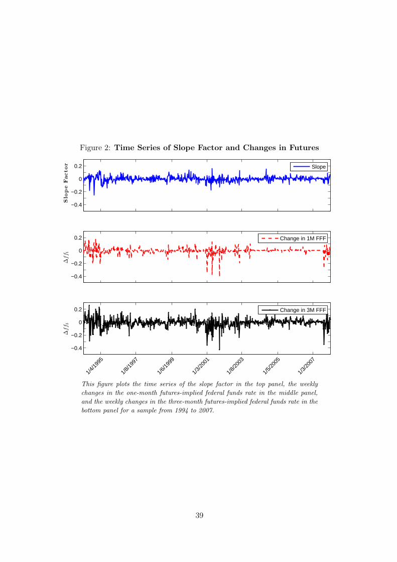
Figure 2: Time Series of Slope Factor and Changes in Futures
−0.4
−0.2
0
0.2
Slo
peFactor
Slope
−0.4
−0.2
0
0.2
∆ff 1
Change in 1M FFF
−0.4
−0.2
0
0.2
∆ff 3
1/4/
1995
1/8/
1997
1/6/
1999
1/3/
2001
1/8/
2003
1/5/
2005
1/3/
2007
Change in 3M FFF
This figure plots the time series of the slope factor in the top panel, the weekly
changes in the one-month futures-implied federal funds rate in the middle panel,
and the weekly changes in the three-month futures-implied federal funds rate in the
bottom panel for a sample from 1994 to 2007.
39
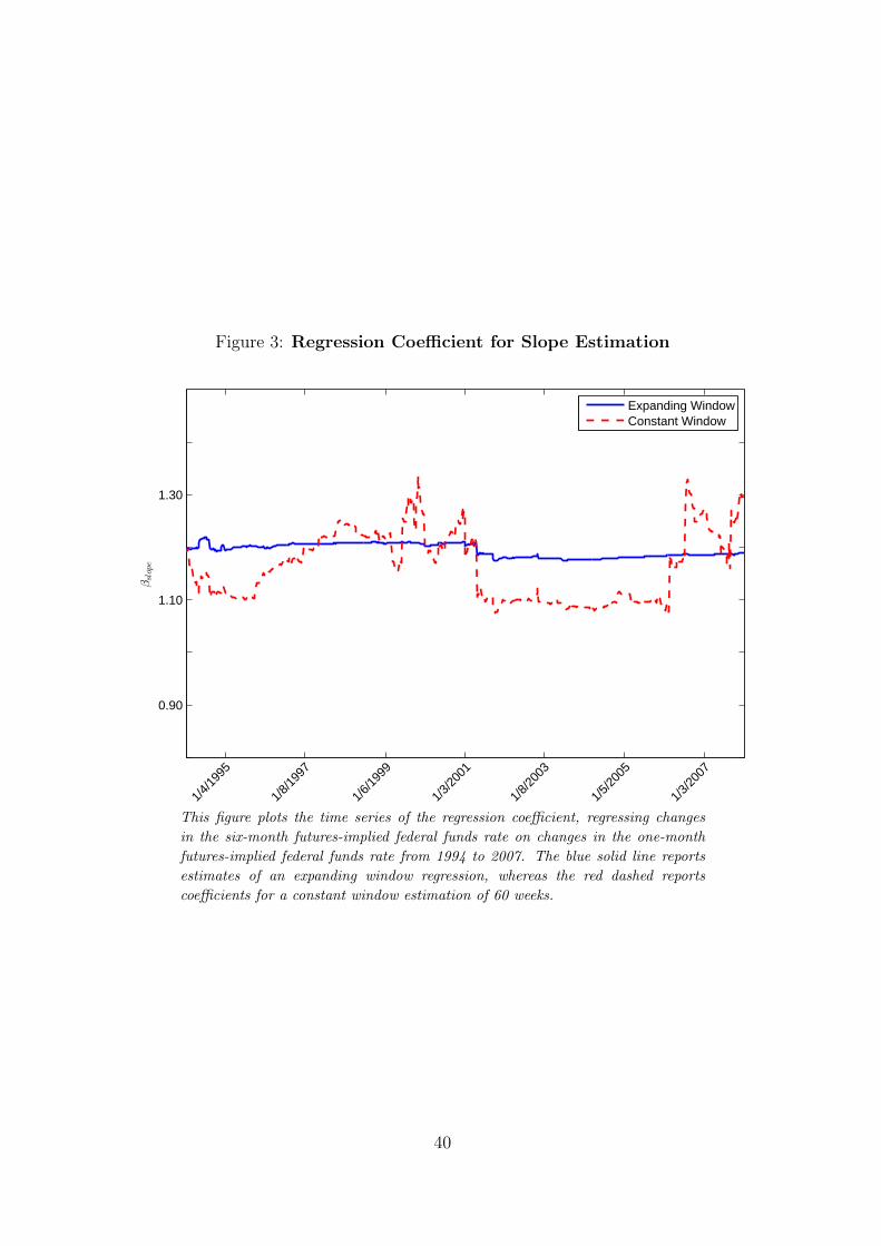
Figure 3: Regression Coefficient for Slope Estimation
0.90
1.10
1.30
βslope
1/4/
1995
1/8/
1997
1/6/
1999
1/3/
2001
1/8/
2003
1/5/
2005
1/3/
2007
Expanding WindowConstant Window
This figure plots the time series of the regression coefficient, regressing changes
in the six-month futures-implied federal funds rate on changes in the one-month
futures-implied federal funds rate from 1994 to 2007. The blue solid line reports
estimates of an expanding window regression, whereas the red dashed reports
coefficients for a constant window estimation of 60 weeks.
40

Table 1: Descriptive Statistics
This table reports descriptive statistics for the slope factor, one- and three-month federal funds futures rates fft,t+1,
one-week changes in these rates, the actual federal funds target rate, the absolute value of the slope factor, and weekly
returns of the CRSP value-weighted index. The sample period is January 1994 to December 2007 for a total of 725
weeks.
Slopet fft,t+1,1 fft,t+1,3 ∆fft,t+1,1 ∆fft,t+1,3 Target Rate abs(Slopet) Rt+1
Mean 0.00 4.23 4.29 -0.01 -0.01 4.20 0.03 0.12
Std (0.04) (1.73) (1.74) (0.05) (0.07) (1.75) (0.03) (2.21)
Nobs 725
41
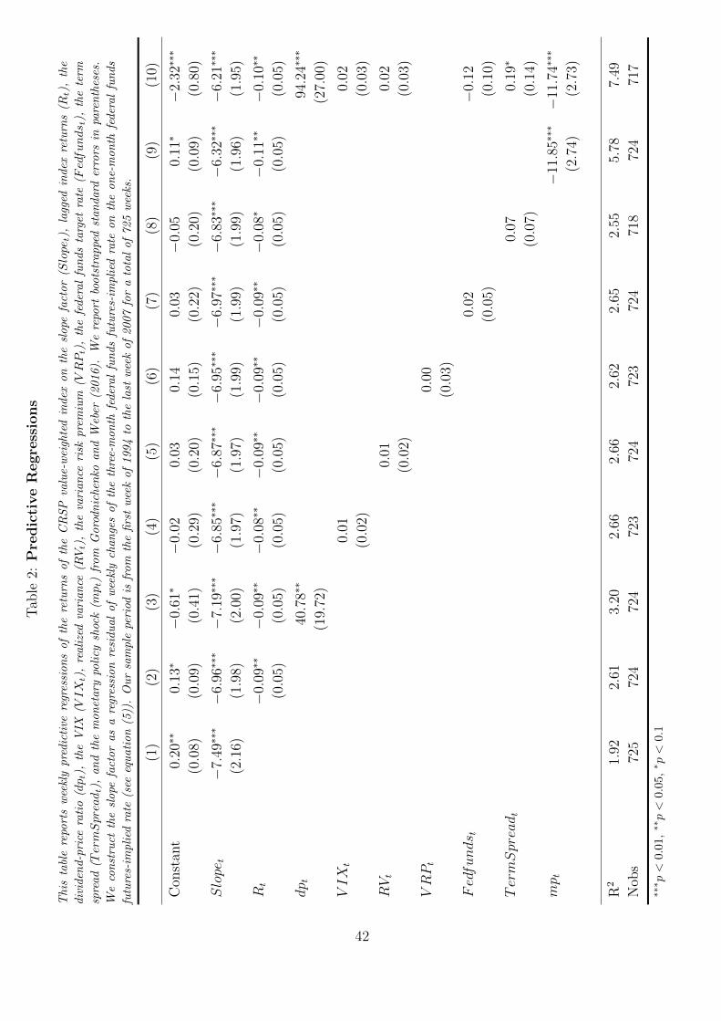
Tab
le2:
Pre
dic
tive
Regre
ssio
ns
This
tabl
ere
port
sw
eekl
ypre
dic
tive
regr
essi
on
sof
the
retu
rns
of
the
CR
SP
valu
e-w
eigh
ted
index
on
the
slope
fact
or
(Slope t
),la
gged
index
retu
rns
(Rt),
the
div
iden
d-p
rice
rati
o(dpt),
the
VIX
(VIX
t),
reali
zed
vari
an
ce(R
Vt),
the
vari
an
ceri
skpre
miu
m(V
RPt),
the
feder
al
fun
ds
targ
etra
te(F
edfunds t
),th
ete
rm
spre
ad
(TermSpreadt),
an
dth
em
on
etary
poli
cysh
ock
(mpt)
from
Goro
dn
ichen
koan
dW
eber
(2016).
We
repo
rtbo
ots
trappe
dst
an
dard
erro
rsin
pare
nth
eses
.
We
con
stru
ctth
esl
ope
fact
or
as
are
gres
sion
resi
du
al
of
wee
kly
chan
ges
of
the
thre
e-m
on
thfe
der
al
fun
ds
futu
res-
impli
edra
teon
the
on
e-m
on
thfe
der
al
fun
ds
futu
res-
impli
edra
te(s
eeeq
uati
on
(5))
.O
ur
sam
ple
peri
odis
from
the
firs
tw
eek
of
1994
toth
ela
stw
eek
of
2007
for
ato
tal
of
725
wee
ks.
(1)
(2)
(3)
(4)
(5)
(6)
(7)
(8)
(9)
(10)
Con
stan
t0.
20∗∗
0.13
∗−
0.61
∗−
0.02
0.03
0.14
0.03
−0.
050.
11∗
−2.
32∗∗
∗
(0.0
8)(0.0
9)(0.4
1)(0.2
9)(0.2
0)(0.1
5)(0.2
2)(0.2
0)(0.0
9)(0.8
0)
Slope
t−
7.49
∗∗∗−
6.96
∗∗∗−
7.19
∗∗∗−
6.85
∗∗∗−
6.87
∗∗∗−
6.95
∗∗∗−
6.97
∗∗∗−
6.83
∗∗∗−
6.32
∗∗∗−
6.21
∗∗∗
(2.1
6)(1.9
8)(2.0
0)(1.9
7)(1.9
7)(1.9
9)(1.9
9)(1.9
9)(1.9
6)(1.9
5)
Rt
−0.
09∗∗
−0.
09∗∗
−0.
08∗∗
−0.
09∗∗
−0.
09∗∗
−0.
09∗∗
−0.
08∗
−0.
11∗∗
−0.
10∗∗
(0.0
5)(0.0
5)(0.0
5)(0.0
5)(0.0
5)(0.0
5)(0.0
5)(0.0
5)(0.0
5)
dp t
40.7
8∗∗
94.2
4∗∗∗
(19.
72)
(27.
00)
VIX
t0.
010.
02
(0.0
2)(0.0
3)
RVt
0.01
0.02
(0.0
2)(0.0
3)
VRPt
0.00
(0.0
3)
Fedfunds t
0.02
−0.
12
(0.0
5)(0.1
0)
TermSpreadt
0.07
0.19
∗
(0.0
7)(0.1
4)
mp t
−11.8
5∗∗∗−
11.7
4∗∗∗
(2.7
4)(2.7
3)
R2
1.92
2.61
3.20
2.66
2.66
2.62
2.65
2.55
5.78
7.49
Nob
s72
572
472
472
372
472
372
471
872
471
7
∗∗∗ p
<0.
01,∗∗p<
0.05
,∗ p
<0.
1
42
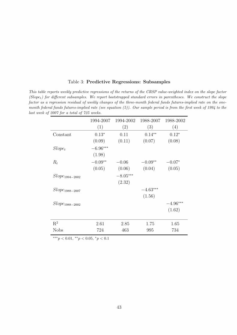
Table 3: Predictive Regressions: Subsamples
This table reports weekly predictive regressions of the returns of the CRSP value-weighted index on the slope factor
(Slopet) for different subsamples. We report bootstrapped standard errors in parentheses. We construct the slope
factor as a regression residual of weekly changes of the three-month federal funds futures-implied rate on the one-
month federal funds futures-implied rate (see equation (5)). Our sample period is from the first week of 1994 to the
last week of 2007 for a total of 725 weeks.
1994-2007 1994-2002 1988-2007 1988-2002
(1) (2) (3) (4)
Constant 0.13∗ 0.11 0.14∗∗ 0.12∗
(0.09) (0.11) (0.07) (0.08)
Slopet −6.96∗∗∗
(1.98)
Rt −0.09∗∗ −0.06 −0.09∗∗ −0.07∗
(0.05) (0.06) (0.04) (0.05)
Slope1994−2002 −8.05∗∗∗
(2.32)
Slope1988−2007 −4.63∗∗∗
(1.56)
Slope1988−2002 −4.96∗∗∗
(1.62)
R2 2.61 2.85 1.75 1.65
Nobs 724 463 995 734
∗∗∗p < 0.01, ∗∗p < 0.05, ∗p < 0.1
43
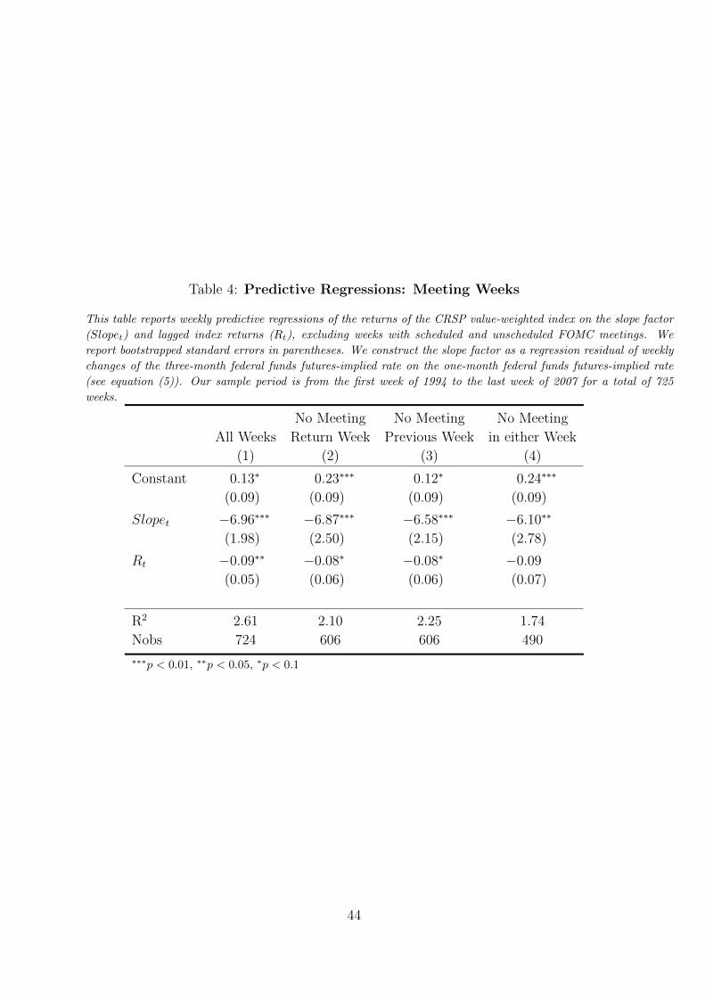
Table 4: Predictive Regressions: Meeting Weeks
This table reports weekly predictive regressions of the returns of the CRSP value-weighted index on the slope factor
(Slopet) and lagged index returns (Rt), excluding weeks with scheduled and unscheduled FOMC meetings. We
report bootstrapped standard errors in parentheses. We construct the slope factor as a regression residual of weekly
changes of the three-month federal funds futures-implied rate on the one-month federal funds futures-implied rate
(see equation (5)). Our sample period is from the first week of 1994 to the last week of 2007 for a total of 725
weeks.
No Meeting No Meeting No Meeting
All Weeks Return Week Previous Week in either Week
(1) (2) (3) (4)
Constant 0.13∗ 0.23∗∗∗ 0.12∗ 0.24∗∗∗
(0.09) (0.09) (0.09) (0.09)
Slopet −6.96∗∗∗ −6.87∗∗∗ −6.58∗∗∗ −6.10∗∗
(1.98) (2.50) (2.15) (2.78)
Rt −0.09∗∗ −0.08∗ −0.08∗ −0.09
(0.05) (0.06) (0.06) (0.07)
R2 2.61 2.10 2.25 1.74
Nobs 724 606 606 490
∗∗∗p < 0.01, ∗∗p < 0.05, ∗p < 0.1
44
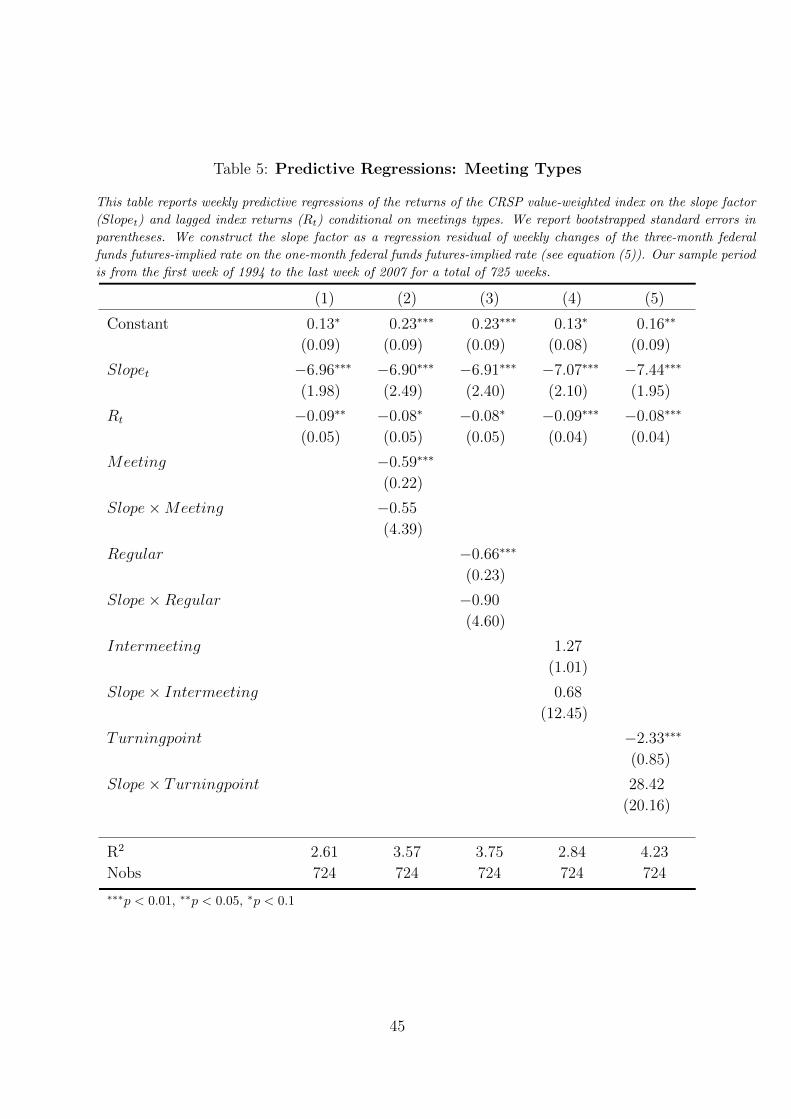
Table 5: Predictive Regressions: Meeting Types
This table reports weekly predictive regressions of the returns of the CRSP value-weighted index on the slope factor
(Slopet) and lagged index returns (Rt) conditional on meetings types. We report bootstrapped standard errors in
parentheses. We construct the slope factor as a regression residual of weekly changes of the three-month federal
funds futures-implied rate on the one-month federal funds futures-implied rate (see equation (5)). Our sample period
is from the first week of 1994 to the last week of 2007 for a total of 725 weeks.
(1) (2) (3) (4) (5)
Constant 0.13∗ 0.23∗∗∗ 0.23∗∗∗ 0.13∗ 0.16∗∗
(0.09) (0.09) (0.09) (0.08) (0.09)
Slopet −6.96∗∗∗ −6.90∗∗∗ −6.91∗∗∗ −7.07∗∗∗ −7.44∗∗∗
(1.98) (2.49) (2.40) (2.10) (1.95)
Rt −0.09∗∗ −0.08∗ −0.08∗ −0.09∗∗∗ −0.08∗∗∗
(0.05) (0.05) (0.05) (0.04) (0.04)
Meeting −0.59∗∗∗
(0.22)
Slope×Meeting −0.55
(4.39)
Regular −0.66∗∗∗
(0.23)
Slope×Regular −0.90
(4.60)
Intermeeting 1.27
(1.01)
Slope× Intermeeting 0.68
(12.45)
Turningpoint −2.33∗∗∗
(0.85)
Slope× Turningpoint 28.42
(20.16)
R2 2.61 3.57 3.75 2.84 4.23
Nobs 724 724 724 724 724
∗∗∗p < 0.01, ∗∗p < 0.05, ∗p < 0.1
45

Table 6: Predictive Regressions: Asymmetries
This table reports weekly predictive regressions of the returns of the CRSP value-weighted index on the slope factor
(Slopet) lagged index returns (Rt) allowing for asymmetric effects of slope: Slope > 0 captures positive values of
the slope factor; Slope <= 0 captures negative values of the slope factor; Slopeupside captures values of the slope
factor larger than one standard deviation above 0; Slopedownside captures values of the slope factor larger than
one standard deviation below 0; Slopenormal captures the intermediate values of slope; Slopelarge captures value of
the slope factor larger than 0.015 in absolute value. We report bootstrapped standard errors in parentheses. We
construct the slope factor as a regression residual of weekly changes of the three-month federal funds futures-implied
rate on the one-month federal funds futures-implied rate (see equation (5)). Our sample period is from the first
week of 1994 to the last week of 2007 for a total of 725 weeks.
(1) (2) (3) (4) (5)
Constant −0.01 0.01 0.05 0.07 0.27∗∗∗
(0.11) (0.11) (0.09) (0.09) (0.11)
Slopet > 0 −2.54 −2.07
(3.67) (3.61)
Slopet <= 0 −12.21∗∗∗ −11.25∗∗∗
(3.62) (3.44)
Rt −0.08∗∗ −0.08∗∗ −0.08∗
(0.05) (0.05) (0.06)
Slopet, normal 7.52 7.84
(6.27) (6.20)
Slopet, upside −3.82 −3.41
(3.47) (3.43)
Slopet, downside −12.08∗∗∗ −11.21∗∗∗
(3.43) (3.27)
Slopet, large −7.33∗∗∗
(1.97)
R2 2.31 2.96 2.34 3.02 4.22
Nobs 725 724 725 724 413
∗∗∗p < 0.01, ∗∗p < 0.05, ∗p < 0.1
46

Table 7: Predictive Regressions: Blackout Periods
This table reports weekly predictive regressions of the returns of the CRSP value-weighted index on the slope
factor (Slopet) and lagged index returns (Rt), excluding weeks during blackout period which restrict the extent
of public communication. We report bootstrapped standard errors in parentheses. We construct the slope factor
as a regression residual of weekly changes of the three-month federal funds futures-implied rate on the one-month
federal funds futures-implied rate (see equation (5)). Our sample period is from the first week of 1994 to the last
week of 2007 for a total of 725 weeks.
No Meeting No Meeting No Meeting
All Weeks Return Week Next Week in either Week
(1) (2) (3) (4)
Constant 0.13∗ 0.23∗ 0.04∗ 0.13∗
(0.09) (0.09) (0.09) (0.09)
Slopet −6.96∗∗∗ −6.87∗∗∗ −6.63∗∗∗ −6.36∗∗∗
(1.98) (1.98) (1.98) (1.98)
Rt −0.09∗∗ −0.08∗∗ −0.07∗∗ −0.08∗∗
(0.05) (0.05) (0.05) (0.05)
R2 2.61 2.10 2.54 2.17
Nobs 724 606 606 490
∗∗∗p < 0.01, ∗∗p < 0.05, ∗p < 0.1
47

Table 8: Predictive Regressions: Target and Path Factor
This table reports weekly predictive regressions of the returns of the CRSP value-weighted index on the slope factor
(Slopet), lagged index returns (Rt), the target (Targetfactor) and path (Pathfactor) from Gurkaynak et al.
(2005b), and the monetary policy shock (mpt) from Gorodnichenko and Weber (2016). We report bootstrapped
standard errors in parentheses. We construct the slope factor as a regression residual of weekly changes of the
three-month federal funds futures-implied rate on the one-month federal funds futures-implied rate (see equation
(5)). Our sample period is from the first week of 1994 to the last week of 2007 for a total of 725 weeks.
(1) (2) (3) (4) (5)
Constant 0.13∗ 0.14∗ 0.13∗ 0.14∗ 0.07
(0.10) (0.10) (0.10) (0.10) (0.10)
Slopet −7.48∗∗∗ −6.93∗∗∗ −7.28∗∗∗ −6.71∗∗∗ −6.66∗∗∗
(2.07) (2.06) (2.04) (2.02) (2.01)
Rt −0.06 −0.08∗ −0.06 −0.08∗ −0.08∗
(0.05) (0.05) (0.05) (0.05) (0.05)
Targetfactor −0.10∗∗∗ −0.10∗∗∗ 0.10
(0.03) (0.03) (0.09)
Pathfactor −0.04∗∗ −0.04∗∗∗ −0.04∗∗∗
(0.02) (0.02) (0.02)
mpt −20.66∗∗∗
(8.14)
R2 2.42 4.57 3.13 5.38 6.76
Nobs 568 568 568 568 568
∗∗∗p < 0.01, ∗∗p < 0.05, ∗p < 0.1
48
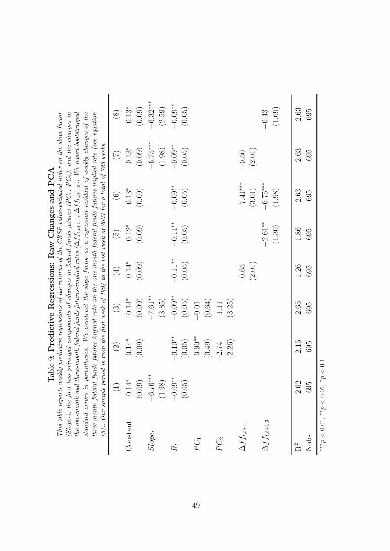
Tab
le9:
Pre
dic
tive
Regre
ssio
ns:
Raw
Changes
and
PC
AT
his
tabl
ere
port
sw
eekl
ypre
dic
tive
regr
essi
on
sof
the
retu
rns
of
the
CR
SP
valu
e-w
eigh
ted
index
on
the
slope
fact
or
(Slope t
),th
efi
rst
two
pri
nci
pal
com
pon
ents
of
chan
ges
infe
der
al
fun
ds
futu
res
(PC
1,PC
2),
an
dth
ech
an
ges
in
the
on
e-m
on
than
dth
ree-
mon
thfe
der
al
fun
ds
futu
res-
impli
edra
tes
(∆ff t
,t+1,1
,∆ff t
,t+1,3
).W
ere
port
boots
trappe
d
stan
dard
erro
rsin
pare
nth
eses
.W
eco
nst
ruct
the
slope
fact
or
as
are
gres
sion
resi
du
al
of
wee
kly
chan
ges
of
the
thre
e-m
on
thfe
der
al
fun
ds
futu
res-
impli
edra
teon
the
on
e-m
on
thfe
der
al
fun
ds
futu
res-
impli
edra
te(s
eeeq
uati
on
(5))
.O
ur
sam
ple
peri
odis
from
the
firs
tw
eek
of
1994
toth
ela
stw
eek
of
2007
for
ato
tal
of
725
wee
ks.
(1)
(2)
(3)
(4)
(5)
(6)
(7)
(8)
Con
stan
t0.
14∗
0.14
∗0.
14∗
0.14
∗0.
12∗
0.13
∗0.
13∗
0.13
∗
(0.0
9)(0.0
9)(0.0
9)(0.0
9)(0.0
9)(0.0
9)(0.0
9)(0.0
9)
Slope
t−
6.76
∗∗∗
−7.
61∗∗
−6.
75∗∗
∗−
6.32
∗∗∗
(1.9
8)(3.8
5)(1.9
8)(2.5
9)
Rt
−0.
09∗∗
−0.
10∗∗
−0.
09∗∗
−0.
11∗∗
−0.
11∗∗
−0.
09∗∗
−0.
09∗∗
−0.
09∗∗
(0.0
5)(0.0
5)(0.0
5)(0.0
5)(0.0
5)(0.0
5)(0.0
5)(0.0
5)
PC
10.
90∗∗
−0.
01
(0.4
9)(0.6
4)
PC
2−
2.74
1.11
(2.2
6)(3.2
5)
∆ff t
,t+1,1
−0.
657.
41∗∗
∗−
0.50
(2.0
1)(3.0
1)(2.0
1)
∆ff t
,t+1,3
−2.
61∗∗
−6.
75∗∗
∗−
0.43
(1.3
0)(1.9
8)(1.6
9)
R2
2.62
2.15
2.65
1.26
1.86
2.63
2.63
2.63
Nob
s69
569
569
569
569
569
569
569
5
∗∗∗ p
<0.
01,∗∗p<
0.05
,∗ p
<0.
1
49

Table 10: Predictive Regressions: Different Horizons
This table reports weekly predictive regressions of the returns of the CRSP value-weighted index on the slope factor
(Slopet) for different forecast horizons running from one week to four weeks. We report bootstrapped standard errors
in parentheses. We construct the slope factor as a regression residual of weekly changes of the three-month federal
funds futures-implied rate on the one-month federal funds futures-implied rate (see equation (5)). Our sample period
is from the first week of 1994 to the last week of 2007 for a total of 725 weeks.
R(t,t+1) R(t,t+2) R(t,t+3) R(t,t+4)
(1) (2) (3) (4)
Constant 0.12∗ 0.23∗∗ 0.33∗∗∗ 0.43∗∗∗
(0.08) (0.11) (0.14) (0.16)
Slopet −7.70∗∗∗ −3.31 −2.83 −5.17∗
(2.07) (3.01) (3.23) (3.84)
R2 1.91 0.19 0.10 0.23
Nobs 725 725 725 725
∗∗∗p < 0.01, ∗∗p < 0.05, ∗p < 0.1
50
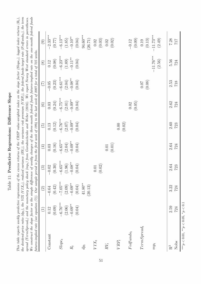
Tab
le11
:P
redic
tive
Regre
ssio
ns:
Diff
ere
nce
Slo
pe
This
tabl
ere
port
sw
eekl
ypre
dic
tive
regr
essi
on
sof
the
exce
ssre
turn
sof
the
CR
SP
valu
e-w
eigh
ted
index
on
the
slope
fact
or
(Slope t
),la
gged
index
retu
rns
(Rt),
the
div
iden
d-p
rice
rati
o(dpt),
the
VIX
(VIX
t),
reali
zed
vari
an
ce(R
Vt),
the
vari
an
ceri
skpre
miu
m(V
RPt),
the
feder
al
fun
ds
targ
etra
te(F
edfunds t
),th
ete
rm
spre
ad
(TermSpreadt)
an
dth
em
on
etary
poli
cysh
ock
(mpt)
fro
mG
oro
dn
ichen
koan
dW
eber
(2016).
We
repo
rtN
ewey
Wes
tst
an
dard
erro
rsin
pare
nth
eses
.
We
con
stru
ctth
esl
ope
fact
or
as
the
sim
ple
diff
eren
ceof
wee
kly
chan
ges
of
the
thre
e-m
on
thfe
der
al
fun
ds
futu
res-
impli
edra
teon
the
on
e-m
on
thfe
der
al
fun
ds
futu
res-
impli
edra
te(s
eeeq
uati
on
(7))
.O
ur
sam
ple
peri
odis
from
the
firs
tw
eek
of
1994
toth
ela
stw
eek
of
2007
for
ato
tal
of
725
wee
ks.
(1)
(2)
(3)
(4)
(5)
(6)
(7)
(8)
(9)
Con
stan
t0.
12−
0.64
−0.
020.
030.
130.
03−
0.05
0.12
−2.
33∗∗
∗
(0.0
9)(0.4
2)(0.3
0)(0.1
6)(0.1
2)(0.2
4)(0.2
3)(0.0
8)(0.7
7)
Slope
t−
6.76
∗∗∗−
7.05
∗∗∗−
6.65
∗∗∗−
6.65
∗∗∗−
6.76
∗∗∗−
6.75
∗∗∗−
6.61
∗∗∗−
6.23
∗∗∗−
6.13
∗∗∗
(2.0
6)(2.0
9)(1.9
6)(2.0
4)(2.0
7)(2.0
1)(2.0
4)(1.8
9)(1.8
5)
Rt
−0.
09∗∗
−0.
09∗∗
−0.
08∗∗
−0.
09∗∗
−0.
09∗∗
−0.
09∗∗
−0.
08∗∗
−0.
11∗∗
−0.
10∗∗
(0.0
4)(0.0
4)(0.0
4)(0.0
4)(0.0
4)(0.0
4)(0.0
4)(0.0
4)(0.0
4)
dp t
41.8
0∗∗
94.6
0∗∗∗
(20.
13)
(26.
71)
VIX
t0.
010.
02
(0.0
2)(0.0
3)
RVt
0.01
0.02
(0.0
1)(0.0
2)
VRPt
0.00
(0.0
2)
Fedfunds t
0.02
−0.
12
(0.0
5)(0.0
9)
TermSpreadt
0.07
0.19
(0.0
8)(0.1
3)
mp t
−11.7
6∗∗∗−
11.7
3∗∗∗
(2.5
6)(2.4
9)
R2
2.59
3.22
2.64
2.64
2.60
2.62
2.53
5.56
7.28
Nob
s72
472
472
372
472
372
471
872
471
7
∗∗∗ p
<0.
01,∗∗p<
0.05
,∗ p
<0.
1
51
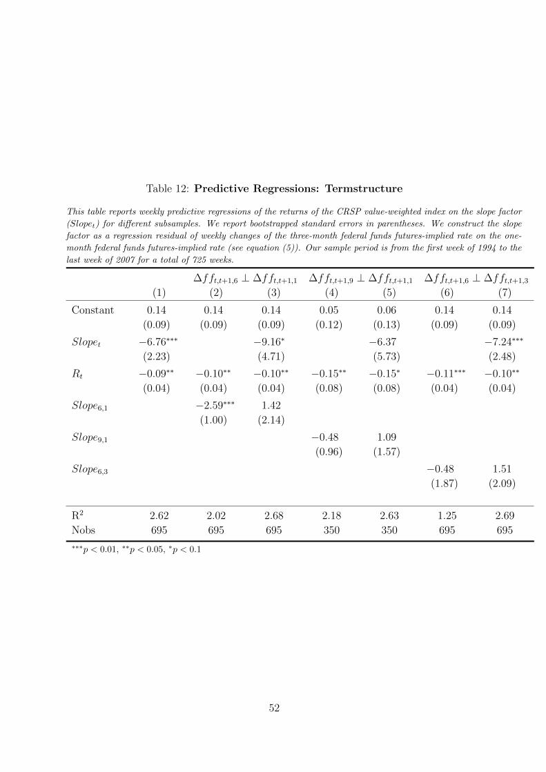
Table 12: Predictive Regressions: Termstructure
This table reports weekly predictive regressions of the returns of the CRSP value-weighted index on the slope factor
(Slopet) for different subsamples. We report bootstrapped standard errors in parentheses. We construct the slope
factor as a regression residual of weekly changes of the three-month federal funds futures-implied rate on the one-
month federal funds futures-implied rate (see equation (5)). Our sample period is from the first week of 1994 to the
last week of 2007 for a total of 725 weeks.
∆fft,t+1,6 ⊥ ∆fft,t+1,1 ∆fft,t+1,9 ⊥ ∆fft,t+1,1 ∆fft,t+1,6 ⊥ ∆fft,t+1,3
(1) (2) (3) (4) (5) (6) (7)
Constant 0.14 0.14 0.14 0.05 0.06 0.14 0.14
(0.09) (0.09) (0.09) (0.12) (0.13) (0.09) (0.09)
Slopet −6.76∗∗∗ −9.16∗ −6.37 −7.24∗∗∗
(2.23) (4.71) (5.73) (2.48)
Rt −0.09∗∗ −0.10∗∗ −0.10∗∗ −0.15∗∗ −0.15∗ −0.11∗∗∗ −0.10∗∗
(0.04) (0.04) (0.04) (0.08) (0.08) (0.04) (0.04)
Slope6,1 −2.59∗∗∗ 1.42
(1.00) (2.14)
Slope9,1 −0.48 1.09
(0.96) (1.57)
Slope6,3 −0.48 1.51
(1.87) (2.09)
R2 2.62 2.02 2.68 2.18 2.63 1.25 2.69
Nobs 695 695 695 350 350 695 695
∗∗∗p < 0.01, ∗∗p < 0.05, ∗p < 0.1
52
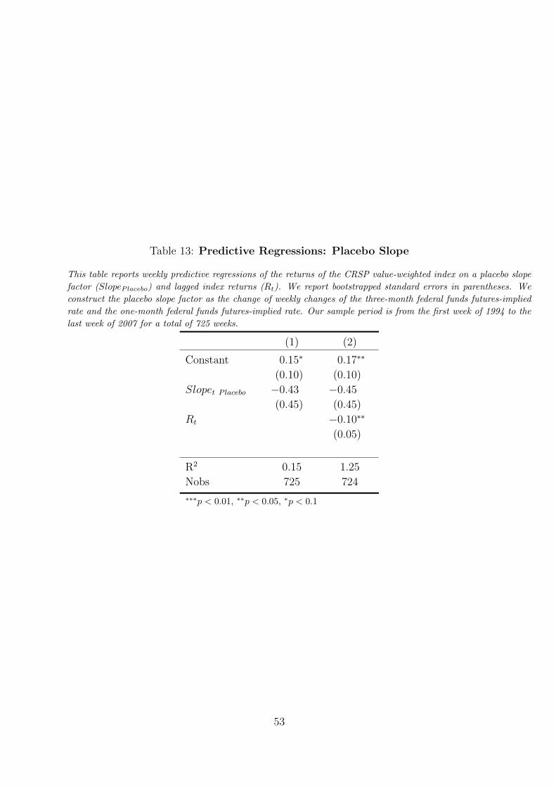
Table 13: Predictive Regressions: Placebo Slope
This table reports weekly predictive regressions of the returns of the CRSP value-weighted index on a placebo slope
factor (SlopePlacebo) and lagged index returns (Rt). We report bootstrapped standard errors in parentheses. We
construct the placebo slope factor as the change of weekly changes of the three-month federal funds futures-implied
rate and the one-month federal funds futures-implied rate. Our sample period is from the first week of 1994 to the
last week of 2007 for a total of 725 weeks.
(1) (2)
Constant 0.15∗ 0.17∗∗
(0.10) (0.10)
Slopet P lacebo −0.43 −0.45
(0.45) (0.45)
Rt −0.10∗∗
(0.05)
R2 0.15 1.25
Nobs 725 724
∗∗∗p < 0.01, ∗∗p < 0.05, ∗p < 0.1
53
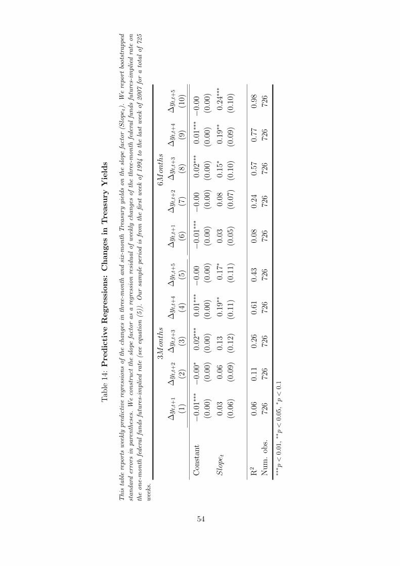
Tab
le14
:P
redic
tive
Regre
ssio
ns:
Changes
inT
reasu
ryY
ield
s
This
tabl
ere
port
sw
eekl
ypre
dic
tive
regr
essi
on
sof
the
chan
ges
inth
ree-
mon
than
dsi
x-m
on
thT
reasu
ryyi
elds
on
the
slope
fact
or
(Slope t
).W
ere
port
boots
tra
ppe
d
stan
dard
erro
rsin
pare
nth
eses
.W
eco
nst
ruct
the
slope
fact
or
as
are
gres
sion
resi
du
al
of
wee
kly
chan
ges
of
the
thre
e-m
on
thfe
der
al
fun
ds
futu
res-
impli
edra
teon
the
on
e-m
on
thfe
der
al
fun
ds
futu
res-
impli
edra
te(s
eeeq
uati
on
(5))
.O
ur
sam
ple
peri
odis
from
the
firs
tw
eek
of
1994
toth
ela
stw
eek
of
2007
for
ato
tal
of
725
wee
ks.
3Months
6Months
∆y t
,t+1
∆y t
,t+2
∆y t
,t+3
∆y t
,t+4
∆y t
,t+5
∆y t
,t+1
∆y t
,t+2
∆y t
,t+3
∆y t
,t+4
∆y t
,t+5
(1)
(2)
(3)
(4)
(5)
(6)
(7)
(8)
(9)
(10)
Con
stan
t−
0.01
∗∗∗−
0.00
∗0.
02∗∗
∗0.
01∗∗
∗−
0.00
−0.
01∗∗
∗−
0.00
0.02
∗∗∗
0.01
∗∗∗−
0.00
(0.0
0)(0.0
0)(0.0
0)(0.0
0)(0.0
0)(0.0
0)(0.0
0)(0.0
0)(0.0
0)(0.0
0)
Slope
t0.
030.
060.
130.
19∗∗
0.17
∗0.
030.
080.
15∗
0.19
∗∗0.
24∗∗
∗
(0.0
6)(0.0
9)(0.1
2)(0.1
1)(0.1
1)(0.0
5)(0.0
7)(0.1
0)(0.0
9)(0.1
0)
R2
0.06
0.11
0.26
0.61
0.43
0.08
0.24
0.57
0.77
0.98
Num
.ob
s.72
672
672
672
672
672
672
672
672
672
6
∗∗∗ p
<0.
01,∗∗p<
0.0
5,∗ p
<0.
1
54
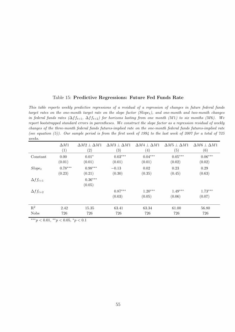
Table 15: Predictive Regressions: Future Fed Funds Rate
This table reports weekly predictive regressions of a residual of a regression of changes in future federal funds
target rates on the one-month target rate on the slope factor (Slopet), and one-month and two-month changes
in federal funds rates (∆fft+1, ∆fft+2) for horizons lasting from one month (M1) to six months (M6). We
report bootstrapped standard errors in parentheses. We construct the slope factor as a regression residual of weekly
changes of the three-month federal funds futures-implied rate on the one-month federal funds futures-implied rate
(see equation (5)). Our sample period is from the first week of 1994 to the last week of 2007 for a total of 725
weeks.
∆M1 ∆M2 ⊥ ∆M1 ∆M3 ⊥ ∆M1 ∆M4 ⊥ ∆M1 ∆M5 ⊥ ∆M1 ∆M6 ⊥ ∆M1
(1) (2) (3) (4) (5) (6)
Constant 0.00 0.01∗ 0.03∗∗∗ 0.04∗∗∗ 0.05∗∗∗ 0.06∗∗∗
(0.01) (0.01) (0.01) (0.01) (0.02) (0.02)
Slopet 0.78∗∗∗ 0.98∗∗∗ −0.13 0.02 0.23 0.29
(0.23) (0.21) (0.30) (0.35) (0.45) (0.63)
∆fft+1 0.36∗∗∗
(0.05)
∆fft+2 0.87∗∗∗ 1.20∗∗∗ 1.49∗∗∗ 1.73∗∗∗
(0.03) (0.05) (0.06) (0.07)
R2 2.42 15.35 63.41 63.34 61.00 56.80
Nobs 726 726 726 726 726 726
∗∗∗p < 0.01, ∗∗p < 0.05, ∗p < 0.1
55

Tab
le16
:L
inguis
tic
Analy
sis
Sp
eech
es
This
tabl
ere
port
sw
eekl
ypre
dic
tive
regr
essi
on
sof
the
slope
fact
or
the
on
eof
spee
ches
bym
embe
rsof
the
FO
MC
.W
e
use
lin
guis
tic
an
aly
sis
toco
un
tth
en
um
ber
of
occu
rren
ces
of
haw
kish
or
dovi
shw
ord
s.T
he
on
lin
eappe
ndix
con
tain
s
ou
rdic
tion
ary
.Hawk−
Dov
eIndex
isa
net
index
that
isla
rger
than
1if
the
spee
chco
nta
ins
more
ha
wki
shth
an
dovi
shte
rms.
Hawk
an
dDov
eco
un
tth
eoc
curr
ence
sof
haw
kish
an
ddovi
shw
ord
s.Chair
isa
du
mm
yth
at
equ
als
1if
asp
eech
isby
the
chair
or
vice
chair
(Chair
).W
ere
port
New
eyW
est
stan
dard
erro
rsin
pare
nth
eses
.W
e
con
stru
ctth
esl
ope
fact
or
as
are
gres
sion
resi
du
al
of
wee
kly
chan
ges
of
the
thre
e-m
on
thfe
der
al
fun
ds
futu
res-
impli
ed
rate
on
the
on
e-m
on
thfe
der
al
fun
ds
futu
res-
impli
edra
te(s
eeeq
uati
on
(5))
.O
ur
sam
ple
peri
odis
from
the
firs
t
wee
kof
19
94
toth
ela
stw
eek
of
2007
for
ato
tal
of
725
wee
ks.
(1)
(2)
(3)
(4)
(5)
(6)
(7)
Con
stan
t−
0.32
−0.
13−
1.56
∗∗∗−
0.68
∗∗−
1.99
∗−
0.94
−0.
18
(0.4
1)(0.2
4)(0.5
9)(0.2
7)(1.1
0)(0.9
0)(0.2
3)
Haw
k-D
ove
Index
0.33
1.06
∗∗1.
73∗∗
(0.3
3)(0.4
5)(0.7
5)
Haw
k0.
090.
56∗∗
∗0.
61∗
0.02
(0.0
5)(0.2
1)(0.3
1)(0.0
7)
Dov
e−
0.09
−0.
30∗
−0.
28∗
0.29
(0.1
6)(0.1
7)(0.1
7)(0.2
5)
Haw
k×
Chai
r0.
43∗
(0.2
2)
Dov
e×
Chai
r−
0.68
∗∗
(0.3
3)
R2
0.21
0.61
2.98
4.60
12.3
812
.35
1.97
Num
.ob
s.38
038
017
317
343
4338
0
Only
Sp
eech
esby
Chai
rX
XX
X
At
leas
t1
clas
sifica
tion
XX
∗∗∗ p
<0.
01,∗∗p<
0.05
,∗ p
<0.
1
56
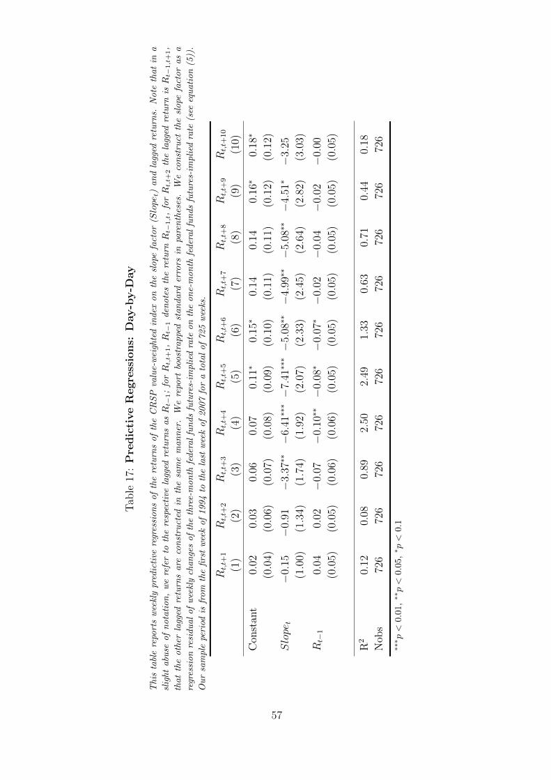
Tab
le17
:P
redic
tive
Regre
ssio
ns:
Day-b
y-D
ay
This
tabl
ere
port
sw
eekl
ypre
dic
tive
regr
essi
on
sof
the
retu
rns
of
the
CR
SP
valu
e-w
eigh
ted
index
on
the
slope
fact
or
(Slope t
)an
dla
gged
retu
rns.
Note
that
ina
slig
ht
abu
seof
nota
tion
,w
ere
fer
toth
ere
spec
tive
lagg
edre
turn
sasR
t−1;
forR
t,t+
1,R
t−1
den
ote
sth
ere
turn
Rt−
1,t
,fo
rR
t,t+
2th
ela
gged
retu
rnis
Rt−
1,t+1,
that
the
oth
erla
gged
retu
rns
are
con
stru
cted
inth
esa
me
man
ner
.W
ere
port
boost
rappe
dst
an
dard
erro
rsin
pare
nth
eses
.W
eco
nst
ruct
the
slope
fact
or
as
a
regr
essi
on
resi
du
al
of
wee
kly
chan
ges
of
the
thre
e-m
on
thfe
der
al
fun
ds
futu
res-
impli
edra
teon
the
on
e-m
on
thfe
der
al
fun
ds
futu
res-
impli
edra
te(s
eeeq
uati
on
(5))
.
Ou
rsa
mple
peri
odis
from
the
firs
tw
eek
of
1994
toth
ela
stw
eek
of
2007
for
ato
tal
of
725
wee
ks.
Rt,t+
1R
t,t+
2R
t,t+
3R
t,t+
4R
t,t+
5R
t,t+
6R
t,t+
7R
t,t+
8R
t,t+
9R
t,t+
10
(1)
(2)
(3)
(4)
(5)
(6)
(7)
(8)
(9)
(10)
Con
stan
t0.
020.
030.
060.
070.
11∗
0.15
∗0.
140.
140.
16∗
0.18
∗
(0.0
4)(0.0
6)(0.0
7)(0.0
8)(0.0
9)(0.1
0)(0.1
1)(0.1
1)(0.1
2)(0.1
2)
Slope
t−
0.15
−0.
91−
3.37
∗∗−
6.41
∗∗∗−
7.41
∗∗∗−
5.08
∗∗−
4.99
∗∗−
5.08
∗∗−
4.51
∗−
3.25
(1.0
0)(1.3
4)(1.7
4)(1.9
2)(2.0
7)(2.3
3)(2.4
5)(2.6
4)(2.8
2)(3.0
3)
Rt−
10.
040.
02−
0.07
−0.
10∗∗−
0.08
∗−
0.07
∗−
0.02
−0.
04−
0.02
−0.
00
(0.0
5)(0.0
5)(0.0
6)(0.0
6)(0.0
5)(0.0
5)(0.0
5)(0.0
5)(0.0
5)(0.0
5)
R2
0.12
0.08
0.89
2.50
2.49
1.33
0.63
0.71
0.44
0.18
Nob
s72
672
672
672
672
672
672
672
672
672
6
∗∗∗ p
<0.0
1,∗∗p<
0.05
,∗ p
<0.
1
57

Table 18: Predictive Regressions: Future Forecast Changes
This table reports monthly predictive regressions of changes in expectations of future fed funds rate on the cumulative
slope factor over the previous three weeks (Slopet−3:t), and the one-month change in expectations for horizons lasting
from one quarter (Q1) to three quarters (Q3). We report Newey-West standard errors in parentheses. We construct
the slope factor as a regression residual of weekly changes of the three-month federal funds futures-implied rate on
the one-month federal funds futures-implied rate (see equation (5)). Our sample period is from the first February
1994 to December of 2007 for a total of 163 months.
∆Q1 ∆Q2 ∆Q3 ∆Q2 ∆Q3
(1) (2) (3) (4) (5)
Constant −0.01 −0.01 −0.02 −0.00 −0.01
(0.02) (0.03) (0.03) (0.01) (0.01)
Slopet−3:t 0.89∗∗∗ 1.02∗∗∗ 1.00∗∗∗ 0.11 0.12
(0.17) (0.16) (0.16) (0.08) (0.12)
∆E fft+1 1.03∗∗∗ 1.00∗∗∗
(0.04) (0.04)
R2 11.32 12.22 11.55 88.26 82.26
Nobs 163 163 163 163 163
∗∗∗p < 0.01, ∗∗p < 0.05, ∗p < 0.1
58

Table 19: Predictive Regressions: Macro News
This table reports weekly predictive regressions of the returns of the CRSP value-weighted index on the slope
factor (Slopet), lagged index returns (Rt) and macro surprises from Haver Analytics: news about GDP growth
(shock gdp), core consumer price inflation (shock cpi), capacity utilization (shock cu ), consumer confidence
(shock cc), employment costs (shock ec), initial unemployment claims (shock ic), the manufacturing composite
index (shock mfg), new home sales (shock nhs), non-farm payroll (shock nfp), core producer price inflation
(shock ppi), retail sales (shock rs), and unemployment (shock ur). We report bootstrapped standard errors in
parentheses. We construct the slope factor as a regression residual of weekly changes of the three-month federal
funds futures-implied rate on the one-month federal funds futures-implied rate (see equation (5)). Our sample period
is from the first week of 1994 to the last week of 2007 for a total of 725 weeks.
(1) (2) (3) (4) (5)
Constant 0.13∗ 0.13∗ 0.12∗ 0.09 −0.00
(0.09) (0.09) (0.09) (0.09) (0.00)
Slopet −6.84∗∗∗ −6.86∗∗∗ −6.74∗∗∗ −6.71∗∗∗
(1.98) (1.99) (1.99) (2.04)
Rt −0.09∗∗ −0.09∗∗ −0.09∗∗ −0.08∗
(0.05) (0.05) (0.05) (0.05)
shock gdp 0.59∗ 0.58∗ 0.55∗ −0.00
(0.37) (0.37) (0.37) (0.01)
shock cpi −1.99 −1.98 −1.43 0.02
(1.58) (1.58) (1.57) (0.04)
shock cu −0.77∗ 0.02∗∗
(0.52) (0.01)
shock cc −0.03 0.00∗∗
(0.04) (0.00)
shock ec 0.04 0.04
(1.56) (0.04)
shock ic −0.00 −0.00∗
(0.00) (0.00)
shock mfg −0.05 0.00∗∗∗
(0.07) (0.00)
shock nhs −0.00 0.00
(0.00) (0.00)
shock nfp −0.00∗∗ 0.00∗∗∗
(0.00) (0.00)
shock ppi 0.58 0.02∗∗
(0.68) (0.01)
shock rs 0.54∗ 0.02∗∗∗
(0.35) (0.01)
shock ur −2.40∗∗ −0.05∗∗
(1.20) (0.02)
R2 2.97 2.76 3.12 5.17 9.23
Nobs 724 724 724 724 726
∗∗∗p < 0.01, ∗∗p < 0.05, ∗p < 0.1
59
Online Appendix:Monetary Policy and the Stock Market: Time-Series
Evidence
Andreas Neuhierl and Michael Weber
Not for Publication
I Lingustic Speech Classification
In applying the search-and-count approach, we first follow procedure often employed in
natural language processing, i.e., we first remove stop words (e.g., “and” or “the”) and
then create stem words.
We collect all speeches for members of the FOMC from
http://www.federalreserve.gov/newsevents/. To classify the tone of speeches, we use a
“search-and-count” approach as in Apel and Grimaldi (2012). Search-and-classify is an
automated method to classify text into categories. The key input into “search-and-count”
classification is a pre-specified word list which the research classifies as “hawkish” or
“dovish.” Using this pre-specified word list, we can count the hawkish and dovish terms
within one speech and aggregate over the document. Following this procedure, we obtain
a classification if a speech is on average more hawkish or dovish.
A subtlety arises in applying the approach of Apel and Grimaldi (2012) to our data
as they work with Swedish texts. In Swedish, compound words such as “output gap”
appear with a blank between the two words. In English many interesting words in our
application are compound words, e.g., “labor force participation.” We therefore first use
a list of such compound words to create a list of relevant nouns to be paired with an
adjective or verb. We then look at all two-grams (contiguous combinations of two words
within a document). We require that one word within a two-gram contains either one of
our nouns or verbs or adjectives. After this filtering step, we obtain a list of two-grams
which we classify into hawkish and dovish. To obtain this classification, we read a large
number of speeches to determine in which context these two-grams are typically used. We
report the classified two-grams and our initial word list available in Table A.1.
1

Table A.1: Hawk–Dove Classification
This table reports the classification of the twograms we use to classify speeches by FOMC members as dovish or
hawkish. Our sample period is from the January 1996 to December 2007.
Dovish Hawkish
anchor inflationexpectations aggregatedemand higher
anchored inflationexpectations assetprices increase
boost aggregatedemand assetprices rise
boost economicactivity businessinvestment increased
cut federalfundsrate declines unemploymentrate
cut interestrates declining unemploymentrate
cuts federalfundsrate drop unemploymentrate
cutting federalfundsrate economicactivity increased
declines assetprices economicoutlook increased
declines crudeoil employment increased
declines economicactivity energyprices rise
declines employment exchangerates lower
declines energyprices gradualincreases federalfundsrate
declines houseprices grossdomesticproduct rising
declines laborforceparticipation growing currentaccountdeficit
declining houseprices higher assetprices
declining interestrates higher employment
downwardpressure assetprices higher energyprices
downwardpressure houseprices higher federalfundsrate
downwardpressure interestrates higher houseprices
drop crudeoil higher inflationexpectations
drop houseprices higher interestrates
easedstance monetarypolicy higher productivitygrowth
easing monetarypolicy higher unitlaborcosts
employment declined houseprices increase
employment fallen houseprices increased
employment fell houseprices rise
employment stable houseprices rising
federalfundsrate lower increase assetprices
firmlyanchored inflationexpectations increase coreinflation
houseprices declined increase currentaccountsurpluses
houseprices fallen increase economicactivity
houseprices fell increase employment
increase aggregatedemand increase energyprices
increase currentaccountdeficit increase federalfundsrate
increase laborproductivity increase houseprices
increase unemploymentrate increase inflationexpectations
increased productivitygrowth increase interestrates
increases laborproductivity increase productivitygrowth
increases productivitygrowth increase resourceutilization
continued on next page
2

Table A.1: Hawk–Dove Classification (continued)
Continued from previous page.
Dovish Hawkish
inflationexpectations anchored increase targetfederalfunds
inflationexpectations declined increase unitlaborcosts
inflationexpectations firmlyanchored increased economicactivity
inflationexpectations remainedstable increased employment
inflationexpectations stable increased laborforceparticipation
inflationexpectations wellanchored increases aggregatedemand
interestrates declined increases assetprices
interestrates drop increases businessinvestment
interestrates easing increases crudeoil
interestrates lower increases employment
interestrates lowering increases energyprices
interestrates remain increases federalfundsrate
keeping interestrates increases houseprices
keeping monetarypolicy increases inflationexpectations
laborproductivity increased increases interestrates
lower energyprices increases outputgap
lower federalfundsrate increases unitlaborcosts
lower houseprices inflationexpectations increased
lower inflationexpectations interestrates higher
lower interestrates interestrates increase
lower levelrealoilprices interestrates increased
lower potentialoutput interestrates mightrise
lowered federalfundsrate interestrates mustrise
lowering federalfundsrate interestrates raise
lowering interestrates interestrates raised
monetarypolicy easing interestrates rise
nonaccelerating inflationrate interestrates rising
productivitygrowth increased lower currentaccountdeficit
productivitygrowth increases lower productivitygrowth
raise aggregatedemand lower unemploymentrate
rapid productivitygains monetarypolicy tightening
reduce federalfundsrate personalsavingrate fallen
reduce interestrates raise federalfundsrate
reduce unemploymentrate raise interestrates
reduced economicactivity raised interestrates
reduced federalfundsrate raising assetprices
reduced interestrates raising federalfundsrate
reducing federalfundsrate raising interestrates
reducing interestrates rapid productivitygrowth
continued on next page
3
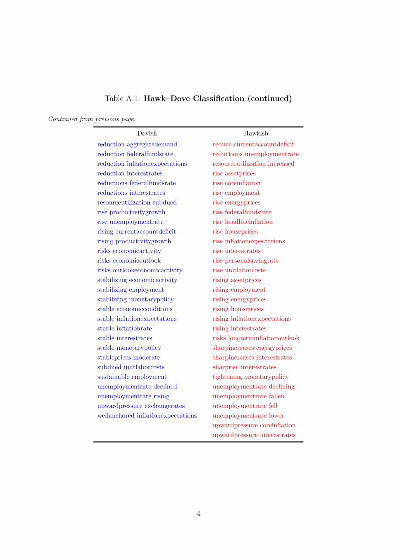
Table A.1: Hawk–Dove Classification (continued)
Continued from previous page.
Dovish Hawkish
reduction aggregatedemand reduce currentaccountdeficit
reduction federalfundsrate reductions unemploymentrate
reduction inflationexpectations resourceutilization increased
reduction interestrates rise assetprices
reductions federalfundsrate rise coreinflation
reductions interestrates rise employment
resourceutilization subdued rise energyprices
rise productivitygrowth rise federalfundsrate
rise unemploymentrate rise headlineinflation
rising currentaccountdeficit rise houseprices
rising productivitygrowth rise inflationexpectations
risks economicactivity rise interestrates
risks economicoutlook rise personalsavingrate
risks outlookeconomicactivity rise unitlaborcosts
stabilizing economicactivity rising assetprices
stabilizing employment rising employment
stabilizing monetarypolicy rising energyprices
stable economicconditions rising houseprices
stable inflationexpectations rising inflationexpectations
stable inflationrate rising interestrates
stable interestrates risks longterminflationoutlook
stable monetarypolicy sharpincreases energyprices
stableprices moderate sharpincreases interestrates
subdued unitlaborcosts sharprise interestrates
sustainable employment tightening monetarypolicy
unemploymentrate declined unemploymentrate declining
unemploymentrate rising unemploymentrate fallen
upwardpressure exchangerates unemploymentrate fell
wellanchored inflationexpectations unemploymentrate lower
upwardpressure coreinflation
upwardpressure interestrates
4
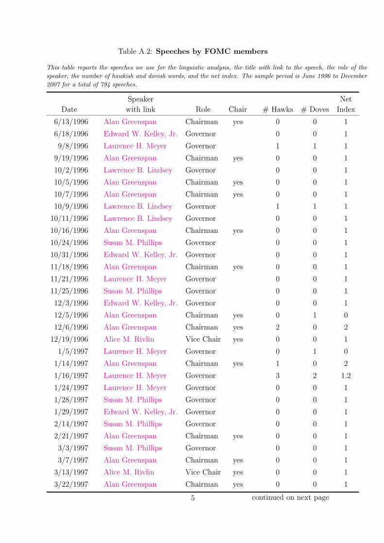
Table A.2: Speeches by FOMC members
This table reports the speeches we use for the linguistic analysis, the title with link to the speech, the role of the
speaker, the number of hawkish and dovish words, and the net index. The sample period is June 1996 to December
2007 for a total of 794 speeches.
Speaker Net
Date with link Role Chair # Hawks # Doves Index
6/13/1996 Alan Greenspan Chairman yes 0 0 1
6/18/1996 Edward W. Kelley, Jr. Governor 0 0 1
9/8/1996 Laurence H. Meyer Governor 1 1 1
9/19/1996 Alan Greenspan Chairman yes 0 0 1
10/2/1996 Lawrence B. Lindsey Governor 0 0 1
10/5/1996 Alan Greenspan Chairman yes 0 0 1
10/7/1996 Alan Greenspan Chairman yes 0 0 1
10/9/1996 Lawrence B. Lindsey Governor 1 1 1
10/11/1996 Lawrence B. Lindsey Governor 0 0 1
10/16/1996 Alan Greenspan Chairman yes 0 0 1
10/24/1996 Susan M. Phillips Governor 0 0 1
10/31/1996 Edward W. Kelley, Jr. Governor 0 0 1
11/18/1996 Alan Greenspan Chairman yes 0 0 1
11/21/1996 Laurence H. Meyer Governor 0 0 1
11/25/1996 Susan M. Phillips Governor 0 0 1
12/3/1996 Edward W. Kelley, Jr. Governor 0 0 1
12/5/1996 Alan Greenspan Chairman yes 0 1 0
12/6/1996 Alan Greenspan Chairman yes 2 0 2
12/19/1996 Alice M. Rivlin Vice Chair yes 0 0 1
1/5/1997 Laurence H. Meyer Governor 0 1 0
1/14/1997 Alan Greenspan Chairman yes 1 0 2
1/16/1997 Laurence H. Meyer Governor 3 2 1.2
1/24/1997 Laurence H. Meyer Governor 0 0 1
1/28/1997 Susan M. Phillips Governor 0 0 1
1/29/1997 Edward W. Kelley, Jr. Governor 0 0 1
2/14/1997 Susan M. Phillips Governor 0 0 1
2/21/1997 Alan Greenspan Chairman yes 0 0 1
3/3/1997 Susan M. Phillips Governor 0 0 1
3/7/1997 Alan Greenspan Chairman yes 0 0 1
3/13/1997 Alice M. Rivlin Vice Chair yes 0 0 1
3/22/1997 Alan Greenspan Chairman yes 0 0 1
continued on next page5
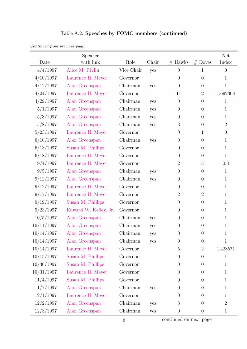
Table A.2: Speeches by FOMC members (continued)
Continued from previous page.
Speaker Net
Date with link Role Chair # Hawks # Doves Index
4/4/1997 Alice M. Rivlin Vice Chair yes 0 1 0
4/10/1997 Laurence H. Meyer Governor 0 0 1
4/12/1997 Alan Greenspan Chairman yes 0 0 1
4/24/1997 Laurence H. Meyer Governor 11 2 1.692308
4/29/1997 Alan Greenspan Chairman yes 0 0 1
5/1/1997 Alan Greenspan Chairman yes 0 0 1
5/3/1997 Alan Greenspan Chairman yes 0 0 1
5/8/1997 Alan Greenspan Chairman yes 3 0 2
5/23/1997 Laurence H. Meyer Governor 0 1 0
6/10/1997 Alan Greenspan Chairman yes 0 0 1
6/18/1997 Susan M. Phillips Governor 0 0 1
6/18/1997 Laurence H. Meyer Governor 0 0 1
9/4/1997 Laurence H. Meyer Governor 2 3 0.8
9/5/1997 Alan Greenspan Chairman yes 0 0 1
9/12/1997 Alan Greenspan Chairman yes 0 0 1
9/12/1997 Laurence H. Meyer Governor 0 0 1
9/17/1997 Laurence H. Meyer Governor 2 2 1
9/19/1997 Susan M. Phillips Governor 0 0 1
9/23/1997 Edward W. Kelley, Jr. Governor 0 0 1
10/5/1997 Alan Greenspan Chairman yes 0 0 1
10/11/1997 Alan Greenspan Chairman yes 0 0 1
10/14/1997 Alan Greenspan Chairman yes 0 0 1
10/14/1997 Alan Greenspan Chairman yes 0 0 1
10/14/1997 Laurence H. Meyer Governor 5 2 1.428571
10/15/1997 Susan M. Phillips Governor 0 0 1
10/30/1997 Susan M. Phillips Governor 0 0 1
10/31/1997 Laurence H. Meyer Governor 0 0 1
11/4/1997 Susan M. Phillips Governor 0 0 1
11/7/1997 Alan Greenspan Chairman yes 0 0 1
12/1/1997 Laurence H. Meyer Governor 0 0 1
12/2/1997 Alan Greenspan Chairman yes 3 0 2
12/3/1997 Alan Greenspan Chairman yes 0 0 1
continued on next page6
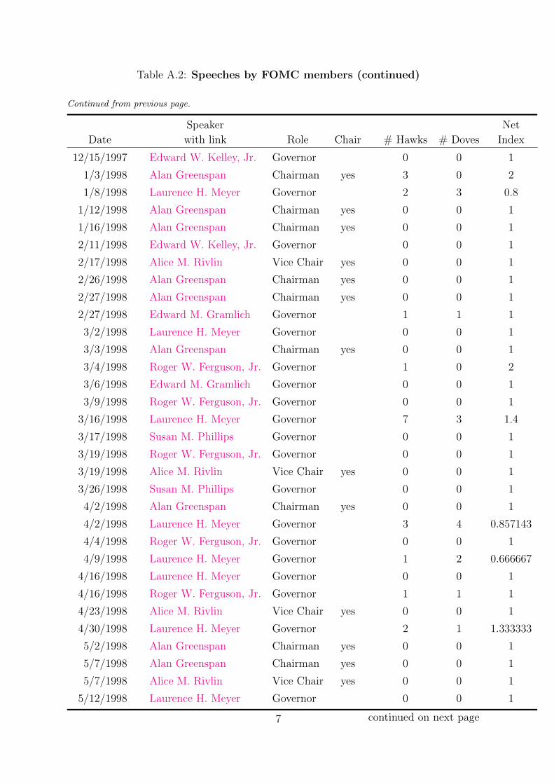
Table A.2: Speeches by FOMC members (continued)
Continued from previous page.
Speaker Net
Date with link Role Chair # Hawks # Doves Index
12/15/1997 Edward W. Kelley, Jr. Governor 0 0 1
1/3/1998 Alan Greenspan Chairman yes 3 0 2
1/8/1998 Laurence H. Meyer Governor 2 3 0.8
1/12/1998 Alan Greenspan Chairman yes 0 0 1
1/16/1998 Alan Greenspan Chairman yes 0 0 1
2/11/1998 Edward W. Kelley, Jr. Governor 0 0 1
2/17/1998 Alice M. Rivlin Vice Chair yes 0 0 1
2/26/1998 Alan Greenspan Chairman yes 0 0 1
2/27/1998 Alan Greenspan Chairman yes 0 0 1
2/27/1998 Edward M. Gramlich Governor 1 1 1
3/2/1998 Laurence H. Meyer Governor 0 0 1
3/3/1998 Alan Greenspan Chairman yes 0 0 1
3/4/1998 Roger W. Ferguson, Jr. Governor 1 0 2
3/6/1998 Edward M. Gramlich Governor 0 0 1
3/9/1998 Roger W. Ferguson, Jr. Governor 0 0 1
3/16/1998 Laurence H. Meyer Governor 7 3 1.4
3/17/1998 Susan M. Phillips Governor 0 0 1
3/19/1998 Roger W. Ferguson, Jr. Governor 0 0 1
3/19/1998 Alice M. Rivlin Vice Chair yes 0 0 1
3/26/1998 Susan M. Phillips Governor 0 0 1
4/2/1998 Alan Greenspan Chairman yes 0 0 1
4/2/1998 Laurence H. Meyer Governor 3 4 0.857143
4/4/1998 Roger W. Ferguson, Jr. Governor 0 0 1
4/9/1998 Laurence H. Meyer Governor 1 2 0.666667
4/16/1998 Laurence H. Meyer Governor 0 0 1
4/16/1998 Roger W. Ferguson, Jr. Governor 1 1 1
4/23/1998 Alice M. Rivlin Vice Chair yes 0 0 1
4/30/1998 Laurence H. Meyer Governor 2 1 1.333333
5/2/1998 Alan Greenspan Chairman yes 0 0 1
5/7/1998 Alan Greenspan Chairman yes 0 0 1
5/7/1998 Alice M. Rivlin Vice Chair yes 0 0 1
5/12/1998 Laurence H. Meyer Governor 0 0 1
continued on next page7
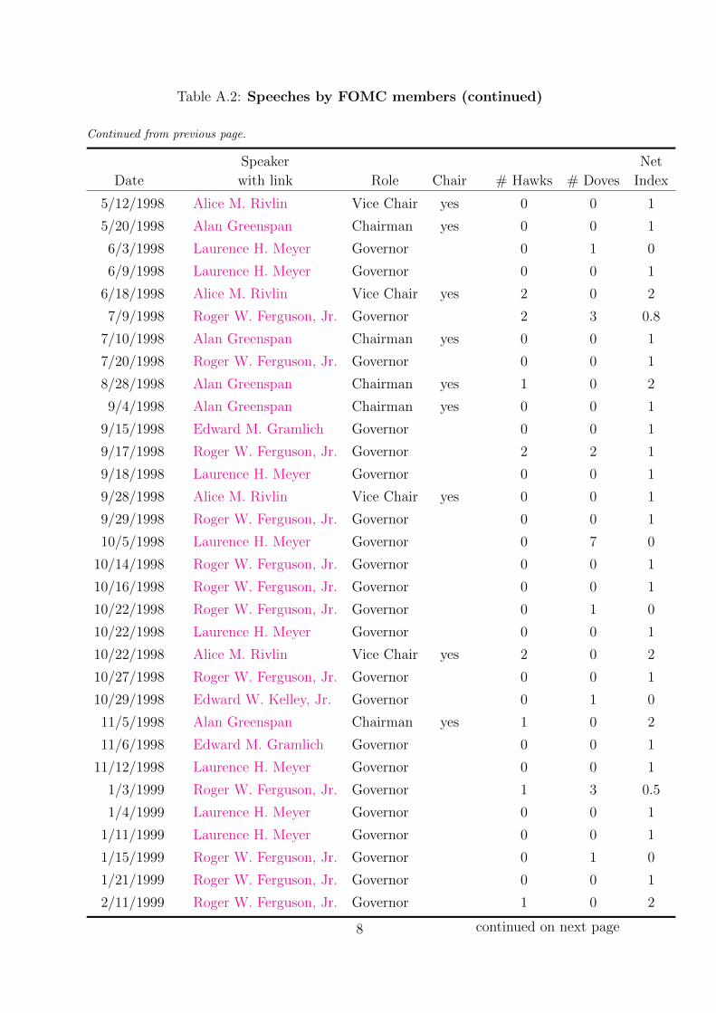
Table A.2: Speeches by FOMC members (continued)
Continued from previous page.
Speaker Net
Date with link Role Chair # Hawks # Doves Index
5/12/1998 Alice M. Rivlin Vice Chair yes 0 0 1
5/20/1998 Alan Greenspan Chairman yes 0 0 1
6/3/1998 Laurence H. Meyer Governor 0 1 0
6/9/1998 Laurence H. Meyer Governor 0 0 1
6/18/1998 Alice M. Rivlin Vice Chair yes 2 0 2
7/9/1998 Roger W. Ferguson, Jr. Governor 2 3 0.8
7/10/1998 Alan Greenspan Chairman yes 0 0 1
7/20/1998 Roger W. Ferguson, Jr. Governor 0 0 1
8/28/1998 Alan Greenspan Chairman yes 1 0 2
9/4/1998 Alan Greenspan Chairman yes 0 0 1
9/15/1998 Edward M. Gramlich Governor 0 0 1
9/17/1998 Roger W. Ferguson, Jr. Governor 2 2 1
9/18/1998 Laurence H. Meyer Governor 0 0 1
9/28/1998 Alice M. Rivlin Vice Chair yes 0 0 1
9/29/1998 Roger W. Ferguson, Jr. Governor 0 0 1
10/5/1998 Laurence H. Meyer Governor 0 7 0
10/14/1998 Roger W. Ferguson, Jr. Governor 0 0 1
10/16/1998 Roger W. Ferguson, Jr. Governor 0 0 1
10/22/1998 Roger W. Ferguson, Jr. Governor 0 1 0
10/22/1998 Laurence H. Meyer Governor 0 0 1
10/22/1998 Alice M. Rivlin Vice Chair yes 2 0 2
10/27/1998 Roger W. Ferguson, Jr. Governor 0 0 1
10/29/1998 Edward W. Kelley, Jr. Governor 0 1 0
11/5/1998 Alan Greenspan Chairman yes 1 0 2
11/6/1998 Edward M. Gramlich Governor 0 0 1
11/12/1998 Laurence H. Meyer Governor 0 0 1
1/3/1999 Roger W. Ferguson, Jr. Governor 1 3 0.5
1/4/1999 Laurence H. Meyer Governor 0 0 1
1/11/1999 Laurence H. Meyer Governor 0 0 1
1/15/1999 Roger W. Ferguson, Jr. Governor 0 1 0
1/21/1999 Roger W. Ferguson, Jr. Governor 0 0 1
2/11/1999 Roger W. Ferguson, Jr. Governor 1 0 2
continued on next page8

Table A.2: Speeches by FOMC members (continued)
Continued from previous page.
Speaker Net
Date with link Role Chair # Hawks # Doves Index
2/16/1999 Alan Greenspan Chairman yes 0 0 1
2/24/1999 Alice M. Rivlin Vice Chair yes 0 0 1
2/25/1999 Laurence H. Meyer Governor 7 6 1.076923
2/25/1999 Roger W. Ferguson, Jr. Governor 0 0 1
3/1/1999 Alice M. Rivlin Vice Chair yes 0 0 1
3/3/1999 Roger W. Ferguson, Jr. Governor 0 0 1
3/8/1999 Edward M. Gramlich Governor 0 0 1
3/8/1999 Alan Greenspan Chairman yes 2 0 2
3/9/1999 Alan Greenspan Chairman yes 0 0 1
3/10/1999 Edward W. Kelley, Jr. Governor 0 0 1
3/12/1999 Laurence H. Meyer Governor 0 0 1
3/16/1999 Alan Greenspan Chairman yes 0 1 0
3/16/1999 Roger W. Ferguson, Jr. Governor 0 0 1
3/19/1999 Alan Greenspan Chairman yes 0 0 1
3/25/1999 Edward W. Kelley, Jr. Governor 0 1 0
4/6/1999 Alice M. Rivlin Vice Chair yes 0 0 1
4/13/1999 Roger W. Ferguson, Jr. Governor 0 0 1
4/14/1999 Laurence H. Meyer Governor 5 4 1.111111
4/16/1999 Alan Greenspan Chairman yes 0 0 1
4/22/1999 Laurence H. Meyer Governor 8 3 1.454545
4/22/1999 Edward M. Gramlich Governor 3 3 1
4/26/1999 Laurence H. Meyer Governor 0 1 0
4/29/1999 Alan Greenspan Chairman yes 1 0 2
5/6/1999 Alan Greenspan Chairman yes 0 2 0
5/13/1999 Alice M. Rivlin Vice Chair yes 0 0 1
5/13/1999 Alice M. Rivlin Vice Chair yes 0 0 1
6/1/1999 Alice M. Rivlin Vice Chair yes 0 0 1
6/2/1999 Alan Greenspan Chairman yes 0 0 1
6/3/1999 Laurence H. Meyer Governor 0 0 1
6/10/1999 Roger W. Ferguson, Jr. Governor 0 1 0
6/10/1999 Alan Greenspan Chairman yes 0 0 1
6/14/1999 Laurence H. Meyer Governor 0 0 1
continued on next page9
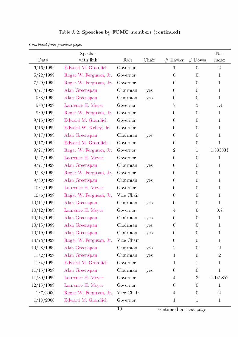
Table A.2: Speeches by FOMC members (continued)
Continued from previous page.
Speaker Net
Date with link Role Chair # Hawks # Doves Index
6/16/1999 Edward M. Gramlich Governor 1 0 2
6/22/1999 Roger W. Ferguson, Jr. Governor 0 0 1
7/29/1999 Roger W. Ferguson, Jr. Governor 0 0 1
8/27/1999 Alan Greenspan Chairman yes 0 0 1
9/8/1999 Alan Greenspan Chairman yes 0 0 1
9/8/1999 Laurence H. Meyer Governor 7 3 1.4
9/9/1999 Roger W. Ferguson, Jr. Governor 0 0 1
9/15/1999 Edward M. Gramlich Governor 0 0 1
9/16/1999 Edward W. Kelley, Jr. Governor 0 0 1
9/17/1999 Alan Greenspan Chairman yes 0 0 1
9/17/1999 Edward M. Gramlich Governor 0 0 1
9/21/1999 Roger W. Ferguson, Jr. Governor 2 1 1.333333
9/27/1999 Laurence H. Meyer Governor 0 0 1
9/27/1999 Alan Greenspan Chairman yes 0 0 1
9/28/1999 Roger W. Ferguson, Jr. Governor 0 0 1
9/30/1999 Alan Greenspan Chairman yes 0 0 1
10/1/1999 Laurence H. Meyer Governor 0 0 1
10/6/1999 Roger W. Ferguson, Jr. Vice Chair 0 0 1
10/11/1999 Alan Greenspan Chairman yes 0 0 1
10/12/1999 Laurence H. Meyer Governor 4 6 0.8
10/14/1999 Alan Greenspan Chairman yes 0 0 1
10/15/1999 Alan Greenspan Chairman yes 0 0 1
10/19/1999 Alan Greenspan Chairman yes 0 0 1
10/28/1999 Roger W. Ferguson, Jr. Vice Chair 0 0 1
10/28/1999 Alan Greenspan Chairman yes 2 0 2
11/2/1999 Alan Greenspan Chairman yes 1 0 2
11/4/1999 Edward M. Gramlich Governor 1 1 1
11/15/1999 Alan Greenspan Chairman yes 0 0 1
11/30/1999 Laurence H. Meyer Governor 4 3 1.142857
12/15/1999 Laurence H. Meyer Governor 0 0 1
1/7/2000 Roger W. Ferguson, Jr. Vice Chair 4 0 2
1/13/2000 Edward M. Gramlich Governor 1 1 1
continued on next page10

Table A.2: Speeches by FOMC members (continued)
Continued from previous page.
Speaker Net
Date with link Role Chair # Hawks # Doves Index
1/13/2000 Alan Greenspan Chairman yes 4 2 1.333333
1/14/2000 Laurence H. Meyer Governor 0 0 1
1/20/2000 Laurence H. Meyer Governor 1 0 2
2/3/2000 Laurence H. Meyer Governor 0 0 1
2/17/2000 Roger W. Ferguson, Jr. Vice Chair 1 1 1
2/23/2000 Laurence H. Meyer Governor 0 1 0
2/25/2000 Laurence H. Meyer Governor 0 0 1
3/3/2000 Laurence H. Meyer Governor 6 1 1.714286
3/6/2000 Alan Greenspan Chairman yes 1 0 2
3/6/2000 Roger W. Ferguson, Jr. Vice Chair 0 0 1
3/7/2000 Edward M. Gramlich Governor 0 0 1
3/8/2000 Alan Greenspan Chairman yes 1 0 2
3/13/2000 Edward M. Gramlich Governor 0 0 1
3/22/2000 Alan Greenspan Chairman yes 0 0 1
3/30/2000 Edward W. Kelley, Jr. Governor 0 0 1
4/5/2000 Alan Greenspan Chairman yes 3 0 2
4/6/2000 Roger W. Ferguson, Jr. Vice Chair 0 0 1
4/7/2000 Alan Greenspan Chairman yes 1 0 2
4/10/2000 Alan Greenspan Chairman yes 0 0 1
4/11/2000 Alan Greenspan Chairman yes 0 0 1
4/12/2000 Laurence H. Meyer Governor 25 2 1.851852
4/14/2000 Alan Greenspan Chairman yes 0 0 1
4/14/2000 Edward M. Gramlich Governor 0 0 1
4/17/2000 Edward M. Gramlich Governor 0 0 1
4/20/2000 Edward M. Gramlich Governor 1 1 1
4/27/2000 Alan Greenspan Chairman yes 1 0 2
5/4/2000 Alan Greenspan Chairman yes 0 0 1
5/4/2000 Roger W. Ferguson, Jr. Vice Chair 0 0 1
5/9/2000 Roger W. Ferguson, Jr. Vice Chair 5 1 1.666667
5/11/2000 Roger W. Ferguson, Jr. Vice Chair 0 1 0
5/12/2000 Roger W. Ferguson, Jr. Vice Chair 0 1 0
5/18/2000 Alan Greenspan Chairman yes 0 0 1
continued on next page11
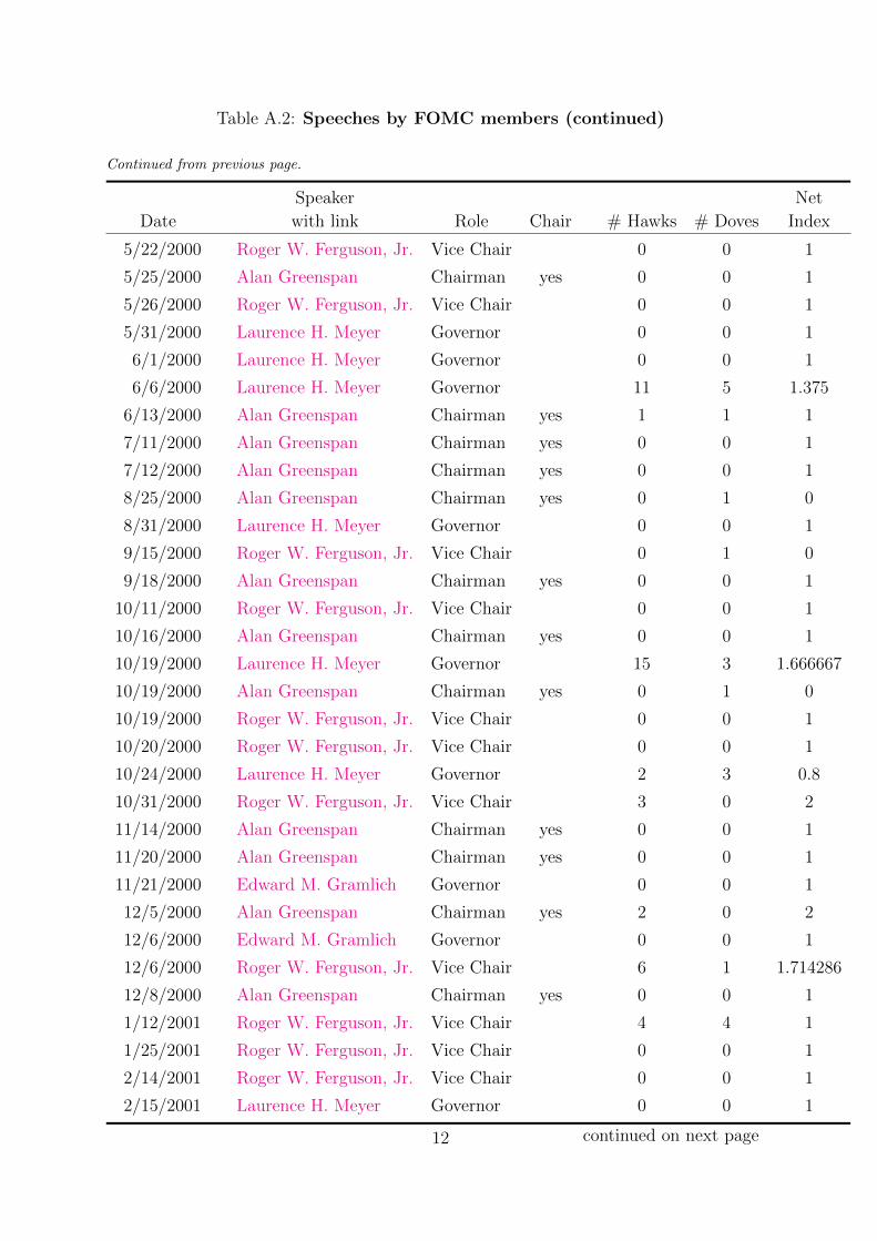
Table A.2: Speeches by FOMC members (continued)
Continued from previous page.
Speaker Net
Date with link Role Chair # Hawks # Doves Index
5/22/2000 Roger W. Ferguson, Jr. Vice Chair 0 0 1
5/25/2000 Alan Greenspan Chairman yes 0 0 1
5/26/2000 Roger W. Ferguson, Jr. Vice Chair 0 0 1
5/31/2000 Laurence H. Meyer Governor 0 0 1
6/1/2000 Laurence H. Meyer Governor 0 0 1
6/6/2000 Laurence H. Meyer Governor 11 5 1.375
6/13/2000 Alan Greenspan Chairman yes 1 1 1
7/11/2000 Alan Greenspan Chairman yes 0 0 1
7/12/2000 Alan Greenspan Chairman yes 0 0 1
8/25/2000 Alan Greenspan Chairman yes 0 1 0
8/31/2000 Laurence H. Meyer Governor 0 0 1
9/15/2000 Roger W. Ferguson, Jr. Vice Chair 0 1 0
9/18/2000 Alan Greenspan Chairman yes 0 0 1
10/11/2000 Roger W. Ferguson, Jr. Vice Chair 0 0 1
10/16/2000 Alan Greenspan Chairman yes 0 0 1
10/19/2000 Laurence H. Meyer Governor 15 3 1.666667
10/19/2000 Alan Greenspan Chairman yes 0 1 0
10/19/2000 Roger W. Ferguson, Jr. Vice Chair 0 0 1
10/20/2000 Roger W. Ferguson, Jr. Vice Chair 0 0 1
10/24/2000 Laurence H. Meyer Governor 2 3 0.8
10/31/2000 Roger W. Ferguson, Jr. Vice Chair 3 0 2
11/14/2000 Alan Greenspan Chairman yes 0 0 1
11/20/2000 Alan Greenspan Chairman yes 0 0 1
11/21/2000 Edward M. Gramlich Governor 0 0 1
12/5/2000 Alan Greenspan Chairman yes 2 0 2
12/6/2000 Edward M. Gramlich Governor 0 0 1
12/6/2000 Roger W. Ferguson, Jr. Vice Chair 6 1 1.714286
12/8/2000 Alan Greenspan Chairman yes 0 0 1
1/12/2001 Roger W. Ferguson, Jr. Vice Chair 4 4 1
1/25/2001 Roger W. Ferguson, Jr. Vice Chair 0 0 1
2/14/2001 Roger W. Ferguson, Jr. Vice Chair 0 0 1
2/15/2001 Laurence H. Meyer Governor 0 0 1
continued on next page12
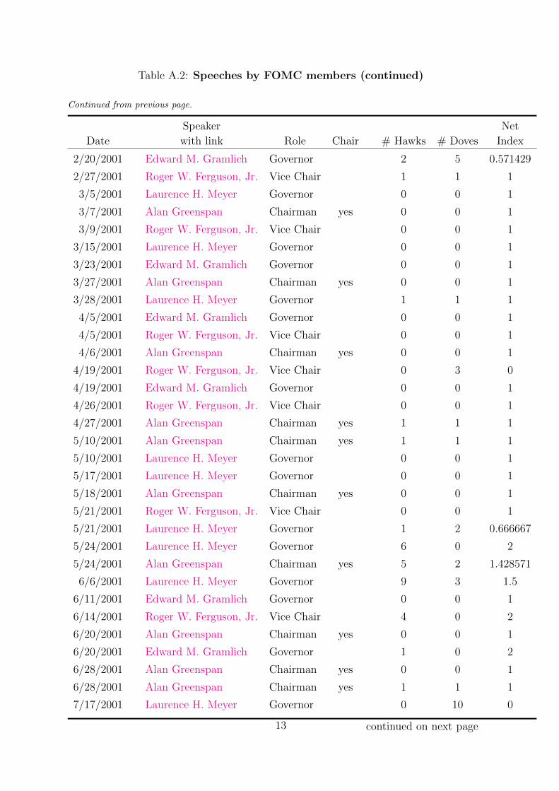
Table A.2: Speeches by FOMC members (continued)
Continued from previous page.
Speaker Net
Date with link Role Chair # Hawks # Doves Index
2/20/2001 Edward M. Gramlich Governor 2 5 0.571429
2/27/2001 Roger W. Ferguson, Jr. Vice Chair 1 1 1
3/5/2001 Laurence H. Meyer Governor 0 0 1
3/7/2001 Alan Greenspan Chairman yes 0 0 1
3/9/2001 Roger W. Ferguson, Jr. Vice Chair 0 0 1
3/15/2001 Laurence H. Meyer Governor 0 0 1
3/23/2001 Edward M. Gramlich Governor 0 0 1
3/27/2001 Alan Greenspan Chairman yes 0 0 1
3/28/2001 Laurence H. Meyer Governor 1 1 1
4/5/2001 Edward M. Gramlich Governor 0 0 1
4/5/2001 Roger W. Ferguson, Jr. Vice Chair 0 0 1
4/6/2001 Alan Greenspan Chairman yes 0 0 1
4/19/2001 Roger W. Ferguson, Jr. Vice Chair 0 3 0
4/19/2001 Edward M. Gramlich Governor 0 0 1
4/26/2001 Roger W. Ferguson, Jr. Vice Chair 0 0 1
4/27/2001 Alan Greenspan Chairman yes 1 1 1
5/10/2001 Alan Greenspan Chairman yes 1 1 1
5/10/2001 Laurence H. Meyer Governor 0 0 1
5/17/2001 Laurence H. Meyer Governor 0 0 1
5/18/2001 Alan Greenspan Chairman yes 0 0 1
5/21/2001 Roger W. Ferguson, Jr. Vice Chair 0 0 1
5/21/2001 Laurence H. Meyer Governor 1 2 0.666667
5/24/2001 Laurence H. Meyer Governor 6 0 2
5/24/2001 Alan Greenspan Chairman yes 5 2 1.428571
6/6/2001 Laurence H. Meyer Governor 9 3 1.5
6/11/2001 Edward M. Gramlich Governor 0 0 1
6/14/2001 Roger W. Ferguson, Jr. Vice Chair 4 0 2
6/20/2001 Alan Greenspan Chairman yes 0 0 1
6/20/2001 Edward M. Gramlich Governor 1 0 2
6/28/2001 Alan Greenspan Chairman yes 0 0 1
6/28/2001 Alan Greenspan Chairman yes 1 1 1
7/17/2001 Laurence H. Meyer Governor 0 10 0
continued on next page13
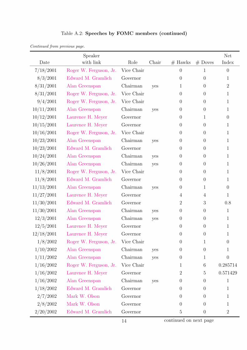
Table A.2: Speeches by FOMC members (continued)
Continued from previous page.
Speaker Net
Date with link Role Chair # Hawks # Doves Index
7/18/2001 Roger W. Ferguson, Jr. Vice Chair 0 1 0
8/3/2001 Edward M. Gramlich Governor 0 0 1
8/31/2001 Alan Greenspan Chairman yes 1 0 2
8/31/2001 Roger W. Ferguson, Jr. Vice Chair 0 0 1
9/4/2001 Roger W. Ferguson, Jr. Vice Chair 0 0 1
10/11/2001 Alan Greenspan Chairman yes 0 0 1
10/12/2001 Laurence H. Meyer Governor 0 1 0
10/15/2001 Laurence H. Meyer Governor 0 0 1
10/16/2001 Roger W. Ferguson, Jr. Vice Chair 0 0 1
10/23/2001 Alan Greenspan Chairman yes 0 0 1
10/23/2001 Edward M. Gramlich Governor 0 0 1
10/24/2001 Alan Greenspan Chairman yes 0 0 1
10/26/2001 Alan Greenspan Chairman yes 0 0 1
11/8/2001 Roger W. Ferguson, Jr. Vice Chair 0 0 1
11/8/2001 Edward M. Gramlich Governor 0 0 1
11/13/2001 Alan Greenspan Chairman yes 0 1 0
11/27/2001 Laurence H. Meyer Governor 4 4 1
11/30/2001 Edward M. Gramlich Governor 2 3 0.8
11/30/2001 Alan Greenspan Chairman yes 0 0 1
12/3/2001 Alan Greenspan Chairman yes 0 0 1
12/5/2001 Laurence H. Meyer Governor 0 0 1
12/18/2001 Laurence H. Meyer Governor 0 0 1
1/8/2002 Roger W. Ferguson, Jr. Vice Chair 0 1 0
1/10/2002 Alan Greenspan Chairman yes 0 0 1
1/11/2002 Alan Greenspan Chairman yes 0 1 0
1/16/2002 Roger W. Ferguson, Jr. Vice Chair 1 6 0.285714
1/16/2002 Laurence H. Meyer Governor 2 5 0.571429
1/16/2002 Alan Greenspan Chairman yes 0 0 1
1/18/2002 Edward M. Gramlich Governor 0 0 1
2/7/2002 Mark W. Olson Governor 0 0 1
2/8/2002 Mark W. Olson Governor 0 0 1
2/20/2002 Edward M. Gramlich Governor 5 0 2
continued on next page14
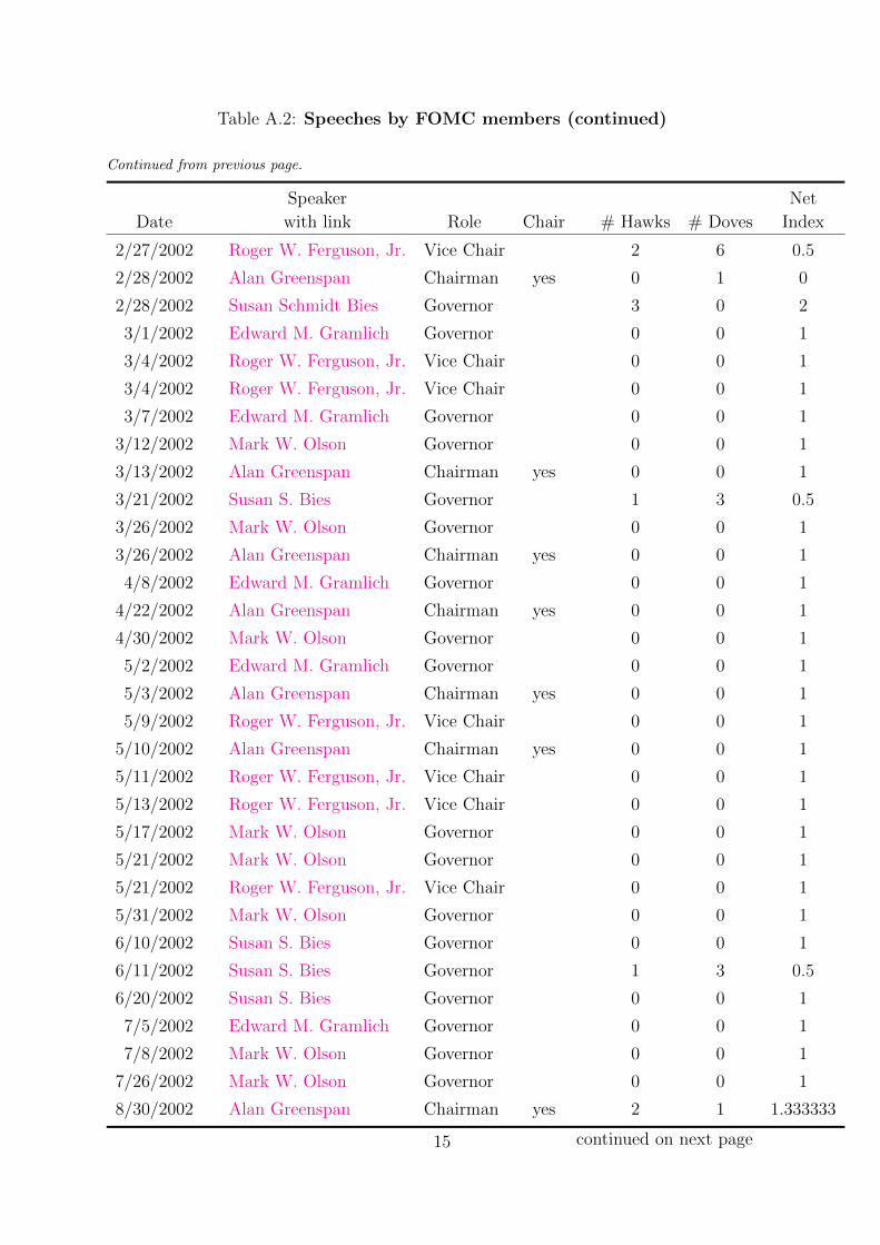
Table A.2: Speeches by FOMC members (continued)
Continued from previous page.
Speaker Net
Date with link Role Chair # Hawks # Doves Index
2/27/2002 Roger W. Ferguson, Jr. Vice Chair 2 6 0.5
2/28/2002 Alan Greenspan Chairman yes 0 1 0
2/28/2002 Susan Schmidt Bies Governor 3 0 2
3/1/2002 Edward M. Gramlich Governor 0 0 1
3/4/2002 Roger W. Ferguson, Jr. Vice Chair 0 0 1
3/4/2002 Roger W. Ferguson, Jr. Vice Chair 0 0 1
3/7/2002 Edward M. Gramlich Governor 0 0 1
3/12/2002 Mark W. Olson Governor 0 0 1
3/13/2002 Alan Greenspan Chairman yes 0 0 1
3/21/2002 Susan S. Bies Governor 1 3 0.5
3/26/2002 Mark W. Olson Governor 0 0 1
3/26/2002 Alan Greenspan Chairman yes 0 0 1
4/8/2002 Edward M. Gramlich Governor 0 0 1
4/22/2002 Alan Greenspan Chairman yes 0 0 1
4/30/2002 Mark W. Olson Governor 0 0 1
5/2/2002 Edward M. Gramlich Governor 0 0 1
5/3/2002 Alan Greenspan Chairman yes 0 0 1
5/9/2002 Roger W. Ferguson, Jr. Vice Chair 0 0 1
5/10/2002 Alan Greenspan Chairman yes 0 0 1
5/11/2002 Roger W. Ferguson, Jr. Vice Chair 0 0 1
5/13/2002 Roger W. Ferguson, Jr. Vice Chair 0 0 1
5/17/2002 Mark W. Olson Governor 0 0 1
5/21/2002 Mark W. Olson Governor 0 0 1
5/21/2002 Roger W. Ferguson, Jr. Vice Chair 0 0 1
5/31/2002 Mark W. Olson Governor 0 0 1
6/10/2002 Susan S. Bies Governor 0 0 1
6/11/2002 Susan S. Bies Governor 1 3 0.5
6/20/2002 Susan S. Bies Governor 0 0 1
7/5/2002 Edward M. Gramlich Governor 0 0 1
7/8/2002 Mark W. Olson Governor 0 0 1
7/26/2002 Mark W. Olson Governor 0 0 1
8/30/2002 Alan Greenspan Chairman yes 2 1 1.333333
continued on next page15

Table A.2: Speeches by FOMC members (continued)
Continued from previous page.
Speaker Net
Date with link Role Chair # Hawks # Doves Index
9/25/2002 Alan Greenspan Chairman yes 0 0 1
9/25/2002 Alan Greenspan Chairman yes 0 0 1
9/25/2002 Alan Greenspan Chairman yes 0 0 1
9/28/2002 Susan S. Bies Governor 1 2 0.666667
10/1/2002 Susan S. Bies Governor 1 0 2
10/3/2002 Roger W. Ferguson, Jr. Vice Chair 0 0 1
10/7/2002 Alan Greenspan Chairman yes 0 0 1
10/8/2002 Susan S. Bies Governor 1 0 2
10/9/2002 Roger W. Ferguson, Jr. Vice Chair 0 0 1
10/15/2002 Ben S. Bernanke Governor 12 2 1.714286
10/16/2002 Roger W. Ferguson, Jr Vice Chair 2 3 0.8
10/16/2002 Roger W. Ferguson, Jr Vice Chair 0 0 1
10/16/2002 Edward M. Gramlich Governor 0 0 1
10/22/2002 Mark W. Olson Governor 0 0 1
10/23/2002 Alan Greenspan Chairman yes 0 0 1
10/24/2002 Roger W. Ferguson, Jr. Vice Chair 0 0 1
10/29/2002 Alan Greenspan Chairman yes 0 0 1
11/7/2002 Susan S. Bies Governor 0 0 1
11/7/2002 Edward M. Gramlich Governor 0 0 1
11/8/2002 Ben S. Bernanke Governor 2 0 2
11/12/2002 Alan Greenspan Chairman yes 0 1 0
11/12/2002 Roger W. Ferguson, Jr. Vice Chair 0 7 0
11/12/2002 Roger W. Ferguson, Jr. Vice Chair 0 1 0
11/12/2002 Mark W. Olson Governor 0 0 1
11/12/2002 Susan S. Bies Governor 0 1 0
11/18/2002 Mark W. Olson Governor 0 0 1
11/18/2002 Alan Greenspan Chairman yes 0 0 1
11/19/2002 Alan Greenspan Chairman yes 0 0 1
11/20/2002 Roger W. Ferguson, Jr. Vice Chair 1 0 2
11/21/2002 Ben S. Bernanke Governor 1 1 1
11/22/2002 Donald L. Kohn Governor 1 1 1
12/13/2002 Susan S. Bies Governor 0 0 1
continued on next page16

Table A.2: Speeches by FOMC members (continued)
Continued from previous page.
Speaker Net
Date with link Role Chair # Hawks # Doves Index
12/13/2002 Mark W. Olson Governor 1 0 2
12/19/2002 Alan Greenspan Chairman yes 1 1 1
1/4/2003 Edward M. Gramlich Governor 1 4 0.4
2/3/2003 Ben S. Bernanke Governor 2 5 0.571429
2/5/2003 Roger W. Ferguson, Jr. Vice Chair 0 0 1
2/6/2003 Mark W. Olson Governor 0 0 1
2/11/2003 Susan Schmidt Bies Governor 3 0 2
2/12/2003 Roger W. Ferguson, Jr Vice Chair 1 2 0.666667
2/21/2003 Ben S. Bernanke Governor 1 3 0.5
2/27/2003 Susan Schmidt Bies Governor 0 0 1
2/28/2003 Donald L. Kohn Governor 10 8 1.111111
3/4/2003 Alan Greenspan Chairman yes 0 0 1
3/7/2003 Alan Greenspan Chairman yes 0 0 1
3/13/2003 Mark W. Olson Governor 0 0 1
3/24/2003 Donald L. Kohn Governor 2 1 1.333333
3/25/2003 Ben S. Bernanke Governor 2 5 0.571429
3/28/2003 Alan Greenspan Chairman yes 0 0 1
4/3/2003 Alan Greenspan Chairman yes 0 0 1
4/4/2003 Alan Greenspan Chairman yes 0 0 1
4/7/2003 Roger W. Ferguson, Jr. Vice Chair 0 0 1
4/9/2003 Roger W. Ferguson, Jr. Vice Chair 0 0 1
4/9/2003 Alan Greenspan Chairman yes 0 0 1
4/10/2003 Mark W. Olson Governor 0 0 1
4/24/2003 Edward M. Gramlich Governor 0 0 1
4/24/2003 Ben S. Bernanke Governor 1 0 2
4/28/2003 Roger W. Ferguson, Jr. Vice Chair 0 0 1
5/7/2003 Susan Schmidt Bies Governor 0 0 1
5/8/2003 Alan Greenspan Chairman yes 0 0 1
5/13/2003 Alan Greenspan Chairman yes 0 0 1
5/16/2003 Roger W. Ferguson, Jr. Vice Chair 0 2 0
5/22/2003 Mark W. Olson Governor 2 1 1.333333
5/30/2003 Susan Schmidt Bies Governor 0 0 1
continued on next page17
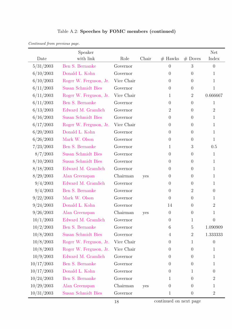
Table A.2: Speeches by FOMC members (continued)
Continued from previous page.
Speaker Net
Date with link Role Chair # Hawks # Doves Index
5/31/2003 Ben S. Bernanke Governor 0 3 0
6/10/2003 Donald L. Kohn Governor 0 0 1
6/10/2003 Roger W. Ferguson, Jr. Vice Chair 0 0 1
6/11/2003 Susan Schmidt Bies Governor 0 0 1
6/11/2003 Roger W. Ferguson, Jr. Vice Chair 1 2 0.666667
6/11/2003 Ben S. Bernanke Governor 0 0 1
6/13/2003 Edward M. Gramlich Governor 2 0 2
6/16/2003 Susan Schmidt Bies Governor 0 0 1
6/17/2003 Roger W. Ferguson, Jr. Vice Chair 0 0 1
6/20/2003 Donald L. Kohn Governor 0 0 1
6/26/2003 Mark W. Olson Governor 0 0 1
7/23/2003 Ben S. Bernanke Governor 1 3 0.5
8/7/2003 Susan Schmidt Bies Governor 0 0 1
8/10/2003 Susan Schmidt Bies Governor 0 0 1
8/18/2003 Edward M. Gramlich Governor 0 0 1
8/29/2003 Alan Greenspan Chairman yes 0 0 1
9/4/2003 Edward M. Gramlich Governor 0 0 1
9/4/2003 Ben S. Bernanke Governor 0 2 0
9/22/2003 Mark W. Olson Governor 0 0 1
9/24/2003 Donald L. Kohn Governor 14 0 2
9/26/2003 Alan Greenspan Chairman yes 0 0 1
10/1/2003 Edward M. Gramlich Governor 0 1 0
10/2/2003 Ben S. Bernanke Governor 6 5 1.090909
10/8/2003 Susan Schmidt Bies Governor 4 2 1.333333
10/8/2003 Roger W. Ferguson, Jr. Vice Chair 0 1 0
10/8/2003 Roger W. Ferguson, Jr. Vice Chair 0 0 1
10/9/2003 Edward M. Gramlich Governor 0 0 1
10/17/2003 Ben S. Bernanke Governor 0 0 1
10/17/2003 Donald L. Kohn Governor 0 1 0
10/24/2003 Ben S. Bernanke Governor 1 0 2
10/29/2003 Alan Greenspan Chairman yes 0 0 1
10/31/2003 Susan Schmidt Bies Governor 1 0 2
continued on next page18
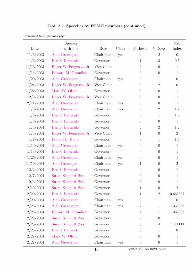
Table A.2: Speeches by FOMC members (continued)
Continued from previous page.
Speaker Net
Date with link Role Chair # Hawks # Doves Index
11/6/2003 Alan Greenspan Chairman yes 0 2 0
11/6/2003 Ben S. Bernanke Governor 1 3 0.5
11/13/2003 Roger W. Ferguson, Jr. Vice Chair 0 0 1
11/14/2003 Edward M. Gramlich Governor 0 0 1
11/20/2003 Alan Greenspan Chairman yes 0 1 0
11/21/2003 Roger W. Ferguson, Jr. Vice Chair 0 2 0
11/22/2003 Mark W. Olson Governor 0 0 1
12/2/2003 Roger W. Ferguson, Jr. Vice Chair 0 0 1
12/11/2003 Alan Greenspan Chairman yes 0 0 1
1/3/2004 Alan Greenspan Chairman yes 3 2 1.2
1/3/2004 Ben S. Bernanke Governor 3 1 1.5
1/3/2004 Ben S. Bernanke Governor 0 0 1
1/4/2004 Ben S. Bernanke Governor 3 2 1.2
1/4/2004 Roger W. Ferguson, Jr. Vice Chair 1 0 2
1/7/2004 Donald L. Kohn Governor 3 1 1.5
1/13/2004 Alan Greenspan Chairman yes 0 0 1
1/14/2004 Ben S. Bernanke Governor 0 0 1
1/26/2004 Alan Greenspan Chairman yes 0 0 1
11/19/2004 Alan Greenspan Chairman yes 1 0 2
12/2/2004 Ben S. Bernanke Governor 0 0 1
12/7/2004 Susan Schmidt Bies Governor 0 0 1
2/4/2004 Susan Schmidt Bies Governor 0 0 1
2/19/2004 Susan Schmidt Bies Governor 1 0 2
2/20/2004 Ben S. Bernanke Governor 1 2 0.666667
2/20/2004 Alan Greenspan Chairman yes 0 1 0
2/23/2004 Alan Greenspan Chairman yes 2 1 1.333333
2/25/2004 Edward M. Gramlich Governor 2 1 1.333333
2/25/2004 Susan Schmidt Bies Governor 0 0 1
2/26/2004 Susan Schmidt Bies Governor 5 4 1.111111
2/26/2004 Ben S. Bernanke Governor 0 1 0
2/27/2004 Mark W. Olson Governor 0 0 1
2/27/2004 Alan Greenspan Chairman yes 0 0 1
continued on next page19
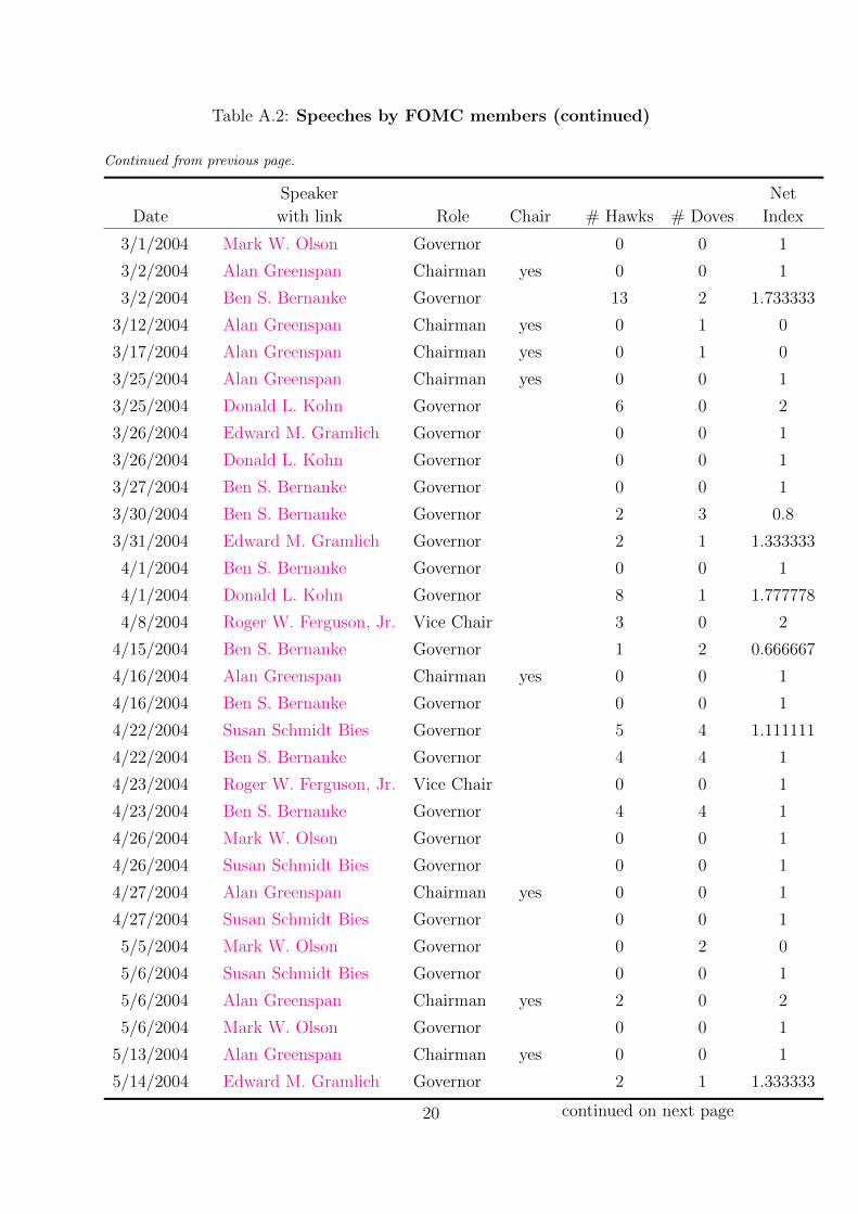
Table A.2: Speeches by FOMC members (continued)
Continued from previous page.
Speaker Net
Date with link Role Chair # Hawks # Doves Index
3/1/2004 Mark W. Olson Governor 0 0 1
3/2/2004 Alan Greenspan Chairman yes 0 0 1
3/2/2004 Ben S. Bernanke Governor 13 2 1.733333
3/12/2004 Alan Greenspan Chairman yes 0 1 0
3/17/2004 Alan Greenspan Chairman yes 0 1 0
3/25/2004 Alan Greenspan Chairman yes 0 0 1
3/25/2004 Donald L. Kohn Governor 6 0 2
3/26/2004 Edward M. Gramlich Governor 0 0 1
3/26/2004 Donald L. Kohn Governor 0 0 1
3/27/2004 Ben S. Bernanke Governor 0 0 1
3/30/2004 Ben S. Bernanke Governor 2 3 0.8
3/31/2004 Edward M. Gramlich Governor 2 1 1.333333
4/1/2004 Ben S. Bernanke Governor 0 0 1
4/1/2004 Donald L. Kohn Governor 8 1 1.777778
4/8/2004 Roger W. Ferguson, Jr. Vice Chair 3 0 2
4/15/2004 Ben S. Bernanke Governor 1 2 0.666667
4/16/2004 Alan Greenspan Chairman yes 0 0 1
4/16/2004 Ben S. Bernanke Governor 0 0 1
4/22/2004 Susan Schmidt Bies Governor 5 4 1.111111
4/22/2004 Ben S. Bernanke Governor 4 4 1
4/23/2004 Roger W. Ferguson, Jr. Vice Chair 0 0 1
4/23/2004 Ben S. Bernanke Governor 4 4 1
4/26/2004 Mark W. Olson Governor 0 0 1
4/26/2004 Susan Schmidt Bies Governor 0 0 1
4/27/2004 Alan Greenspan Chairman yes 0 0 1
4/27/2004 Susan Schmidt Bies Governor 0 0 1
5/5/2004 Mark W. Olson Governor 0 2 0
5/6/2004 Susan Schmidt Bies Governor 0 0 1
5/6/2004 Alan Greenspan Chairman yes 2 0 2
5/6/2004 Mark W. Olson Governor 0 0 1
5/13/2004 Alan Greenspan Chairman yes 0 0 1
5/14/2004 Edward M. Gramlich Governor 2 1 1.333333
continued on next page20
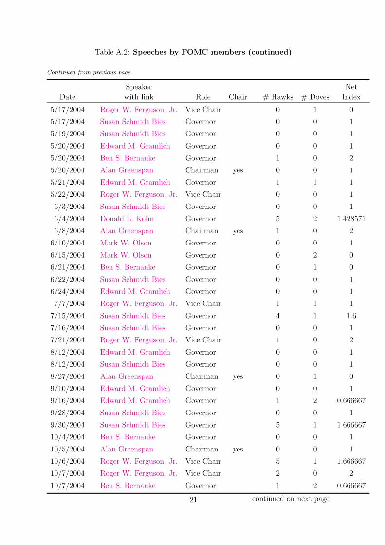
Table A.2: Speeches by FOMC members (continued)
Continued from previous page.
Speaker Net
Date with link Role Chair # Hawks # Doves Index
5/17/2004 Roger W. Ferguson, Jr. Vice Chair 0 1 0
5/17/2004 Susan Schmidt Bies Governor 0 0 1
5/19/2004 Susan Schmidt Bies Governor 0 0 1
5/20/2004 Edward M. Gramlich Governor 0 0 1
5/20/2004 Ben S. Bernanke Governor 1 0 2
5/20/2004 Alan Greenspan Chairman yes 0 0 1
5/21/2004 Edward M. Gramlich Governor 1 1 1
5/22/2004 Roger W. Ferguson, Jr. Vice Chair 0 0 1
6/3/2004 Susan Schmidt Bies Governor 0 0 1
6/4/2004 Donald L. Kohn Governor 5 2 1.428571
6/8/2004 Alan Greenspan Chairman yes 1 0 2
6/10/2004 Mark W. Olson Governor 0 0 1
6/15/2004 Mark W. Olson Governor 0 2 0
6/21/2004 Ben S. Bernanke Governor 0 1 0
6/22/2004 Susan Schmidt Bies Governor 0 0 1
6/24/2004 Edward M. Gramlich Governor 0 0 1
7/7/2004 Roger W. Ferguson, Jr. Vice Chair 1 1 1
7/15/2004 Susan Schmidt Bies Governor 4 1 1.6
7/16/2004 Susan Schmidt Bies Governor 0 0 1
7/21/2004 Roger W. Ferguson, Jr. Vice Chair 1 0 2
8/12/2004 Edward M. Gramlich Governor 0 0 1
8/12/2004 Susan Schmidt Bies Governor 0 0 1
8/27/2004 Alan Greenspan Chairman yes 0 1 0
9/10/2004 Edward M. Gramlich Governor 0 0 1
9/16/2004 Edward M. Gramlich Governor 1 2 0.666667
9/28/2004 Susan Schmidt Bies Governor 0 0 1
9/30/2004 Susan Schmidt Bies Governor 5 1 1.666667
10/4/2004 Ben S. Bernanke Governor 0 0 1
10/5/2004 Alan Greenspan Chairman yes 0 0 1
10/6/2004 Roger W. Ferguson, Jr. Vice Chair 5 1 1.666667
10/7/2004 Roger W. Ferguson, Jr. Vice Chair 2 0 2
10/7/2004 Ben S. Bernanke Governor 1 2 0.666667
continued on next page21
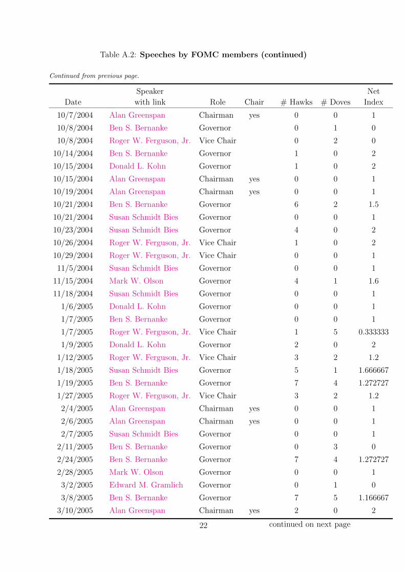
Table A.2: Speeches by FOMC members (continued)
Continued from previous page.
Speaker Net
Date with link Role Chair # Hawks # Doves Index
10/7/2004 Alan Greenspan Chairman yes 0 0 1
10/8/2004 Ben S. Bernanke Governor 0 1 0
10/8/2004 Roger W. Ferguson, Jr. Vice Chair 0 2 0
10/14/2004 Ben S. Bernanke Governor 1 0 2
10/15/2004 Donald L. Kohn Governor 1 0 2
10/15/2004 Alan Greenspan Chairman yes 0 0 1
10/19/2004 Alan Greenspan Chairman yes 0 0 1
10/21/2004 Ben S. Bernanke Governor 6 2 1.5
10/21/2004 Susan Schmidt Bies Governor 0 0 1
10/23/2004 Susan Schmidt Bies Governor 4 0 2
10/26/2004 Roger W. Ferguson, Jr. Vice Chair 1 0 2
10/29/2004 Roger W. Ferguson, Jr. Vice Chair 0 0 1
11/5/2004 Susan Schmidt Bies Governor 0 0 1
11/15/2004 Mark W. Olson Governor 4 1 1.6
11/18/2004 Susan Schmidt Bies Governor 0 0 1
1/6/2005 Donald L. Kohn Governor 0 0 1
1/7/2005 Ben S. Bernanke Governor 0 0 1
1/7/2005 Roger W. Ferguson, Jr. Vice Chair 1 5 0.333333
1/9/2005 Donald L. Kohn Governor 2 0 2
1/12/2005 Roger W. Ferguson, Jr. Vice Chair 3 2 1.2
1/18/2005 Susan Schmidt Bies Governor 5 1 1.666667
1/19/2005 Ben S. Bernanke Governor 7 4 1.272727
1/27/2005 Roger W. Ferguson, Jr. Vice Chair 3 2 1.2
2/4/2005 Alan Greenspan Chairman yes 0 0 1
2/6/2005 Alan Greenspan Chairman yes 0 0 1
2/7/2005 Susan Schmidt Bies Governor 0 0 1
2/11/2005 Ben S. Bernanke Governor 0 3 0
2/24/2005 Ben S. Bernanke Governor 7 4 1.272727
2/28/2005 Mark W. Olson Governor 0 0 1
3/2/2005 Edward M. Gramlich Governor 0 1 0
3/8/2005 Ben S. Bernanke Governor 7 5 1.166667
3/10/2005 Alan Greenspan Chairman yes 2 0 2
continued on next page22
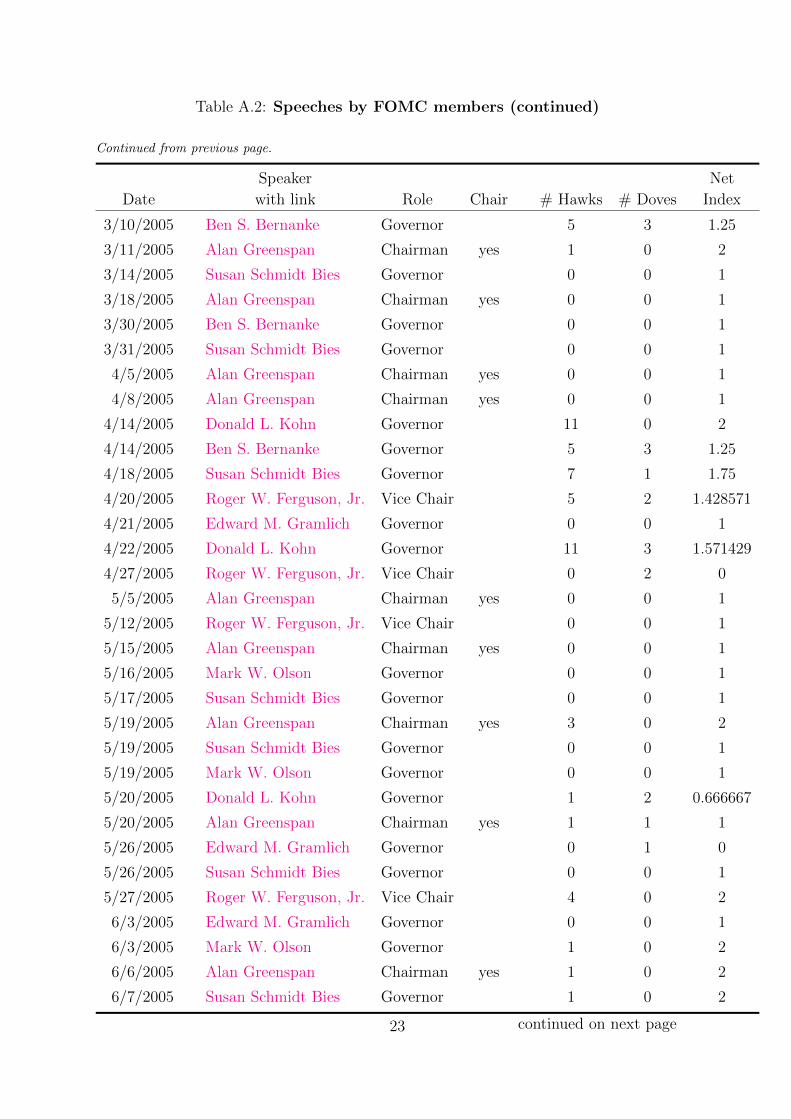
Table A.2: Speeches by FOMC members (continued)
Continued from previous page.
Speaker Net
Date with link Role Chair # Hawks # Doves Index
3/10/2005 Ben S. Bernanke Governor 5 3 1.25
3/11/2005 Alan Greenspan Chairman yes 1 0 2
3/14/2005 Susan Schmidt Bies Governor 0 0 1
3/18/2005 Alan Greenspan Chairman yes 0 0 1
3/30/2005 Ben S. Bernanke Governor 0 0 1
3/31/2005 Susan Schmidt Bies Governor 0 0 1
4/5/2005 Alan Greenspan Chairman yes 0 0 1
4/8/2005 Alan Greenspan Chairman yes 0 0 1
4/14/2005 Donald L. Kohn Governor 11 0 2
4/14/2005 Ben S. Bernanke Governor 5 3 1.25
4/18/2005 Susan Schmidt Bies Governor 7 1 1.75
4/20/2005 Roger W. Ferguson, Jr. Vice Chair 5 2 1.428571
4/21/2005 Edward M. Gramlich Governor 0 0 1
4/22/2005 Donald L. Kohn Governor 11 3 1.571429
4/27/2005 Roger W. Ferguson, Jr. Vice Chair 0 2 0
5/5/2005 Alan Greenspan Chairman yes 0 0 1
5/12/2005 Roger W. Ferguson, Jr. Vice Chair 0 0 1
5/15/2005 Alan Greenspan Chairman yes 0 0 1
5/16/2005 Mark W. Olson Governor 0 0 1
5/17/2005 Susan Schmidt Bies Governor 0 0 1
5/19/2005 Alan Greenspan Chairman yes 3 0 2
5/19/2005 Susan Schmidt Bies Governor 0 0 1
5/19/2005 Mark W. Olson Governor 0 0 1
5/20/2005 Donald L. Kohn Governor 1 2 0.666667
5/20/2005 Alan Greenspan Chairman yes 1 1 1
5/26/2005 Edward M. Gramlich Governor 0 1 0
5/26/2005 Susan Schmidt Bies Governor 0 0 1
5/27/2005 Roger W. Ferguson, Jr. Vice Chair 4 0 2
6/3/2005 Edward M. Gramlich Governor 0 0 1
6/3/2005 Mark W. Olson Governor 1 0 2
6/6/2005 Alan Greenspan Chairman yes 1 0 2
6/7/2005 Susan Schmidt Bies Governor 1 0 2
continued on next page23
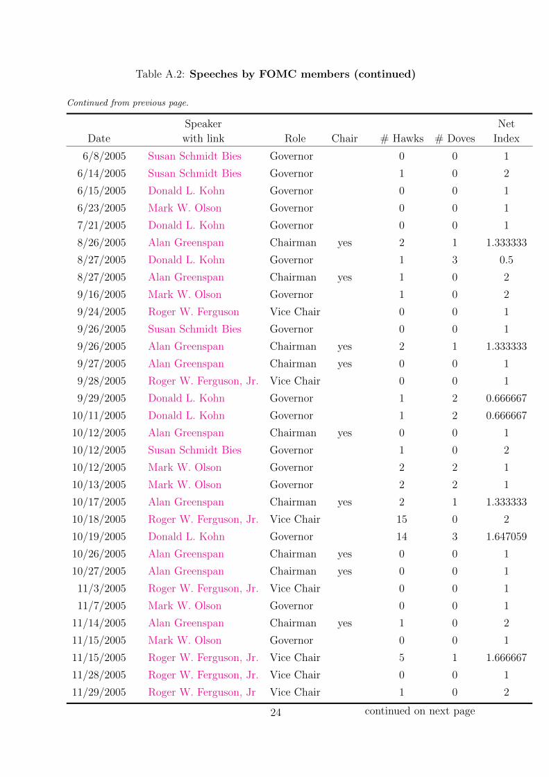
Table A.2: Speeches by FOMC members (continued)
Continued from previous page.
Speaker Net
Date with link Role Chair # Hawks # Doves Index
6/8/2005 Susan Schmidt Bies Governor 0 0 1
6/14/2005 Susan Schmidt Bies Governor 1 0 2
6/15/2005 Donald L. Kohn Governor 0 0 1
6/23/2005 Mark W. Olson Governor 0 0 1
7/21/2005 Donald L. Kohn Governor 0 0 1
8/26/2005 Alan Greenspan Chairman yes 2 1 1.333333
8/27/2005 Donald L. Kohn Governor 1 3 0.5
8/27/2005 Alan Greenspan Chairman yes 1 0 2
9/16/2005 Mark W. Olson Governor 1 0 2
9/24/2005 Roger W. Ferguson Vice Chair 0 0 1
9/26/2005 Susan Schmidt Bies Governor 0 0 1
9/26/2005 Alan Greenspan Chairman yes 2 1 1.333333
9/27/2005 Alan Greenspan Chairman yes 0 0 1
9/28/2005 Roger W. Ferguson, Jr. Vice Chair 0 0 1
9/29/2005 Donald L. Kohn Governor 1 2 0.666667
10/11/2005 Donald L. Kohn Governor 1 2 0.666667
10/12/2005 Alan Greenspan Chairman yes 0 0 1
10/12/2005 Susan Schmidt Bies Governor 1 0 2
10/12/2005 Mark W. Olson Governor 2 2 1
10/13/2005 Mark W. Olson Governor 2 2 1
10/17/2005 Alan Greenspan Chairman yes 2 1 1.333333
10/18/2005 Roger W. Ferguson, Jr. Vice Chair 15 0 2
10/19/2005 Donald L. Kohn Governor 14 3 1.647059
10/26/2005 Alan Greenspan Chairman yes 0 0 1
10/27/2005 Alan Greenspan Chairman yes 0 0 1
11/3/2005 Roger W. Ferguson, Jr. Vice Chair 0 0 1
11/7/2005 Mark W. Olson Governor 0 0 1
11/14/2005 Alan Greenspan Chairman yes 1 0 2
11/15/2005 Mark W. Olson Governor 0 0 1
11/15/2005 Roger W. Ferguson, Jr. Vice Chair 5 1 1.666667
11/28/2005 Roger W. Ferguson, Jr. Vice Chair 0 0 1
11/29/2005 Roger W. Ferguson, Jr Vice Chair 1 0 2
continued on next page24
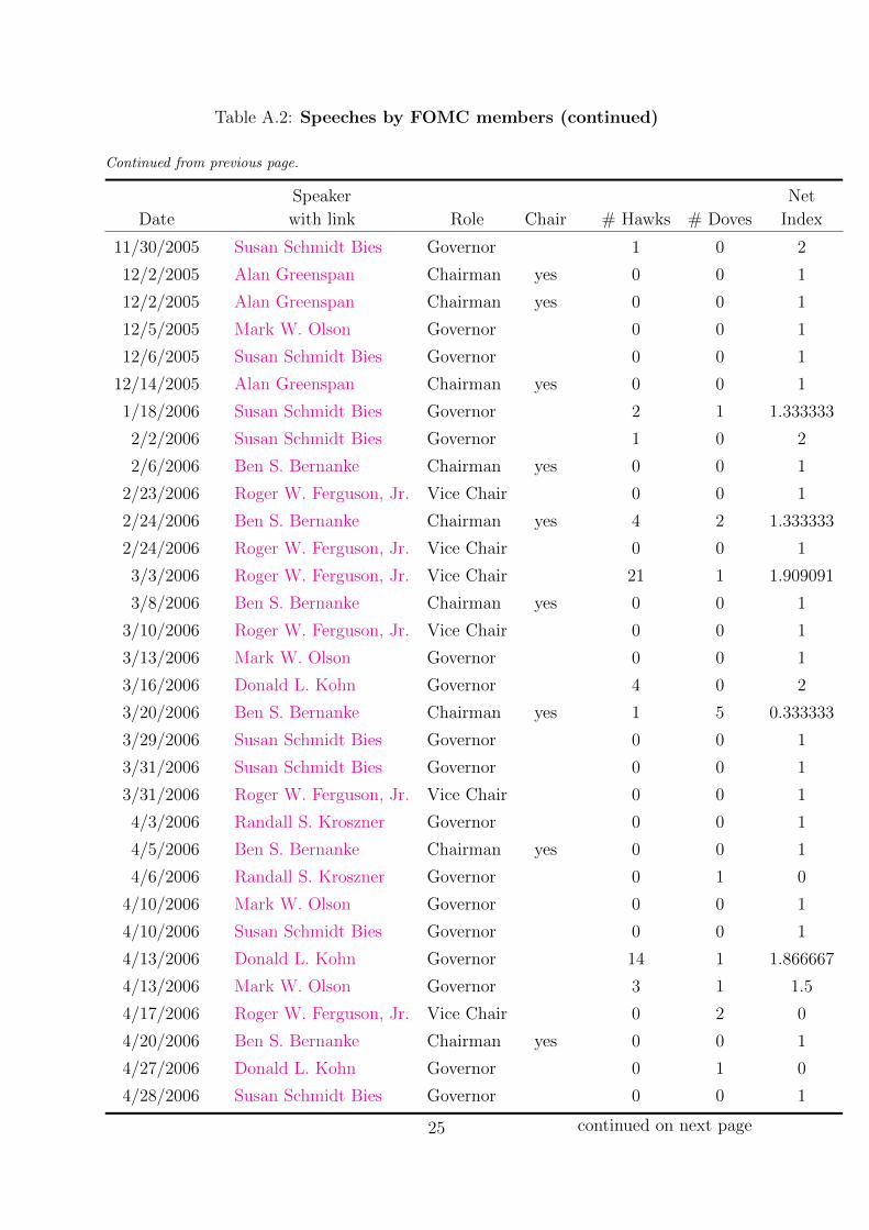
Table A.2: Speeches by FOMC members (continued)
Continued from previous page.
Speaker Net
Date with link Role Chair # Hawks # Doves Index
11/30/2005 Susan Schmidt Bies Governor 1 0 2
12/2/2005 Alan Greenspan Chairman yes 0 0 1
12/2/2005 Alan Greenspan Chairman yes 0 0 1
12/5/2005 Mark W. Olson Governor 0 0 1
12/6/2005 Susan Schmidt Bies Governor 0 0 1
12/14/2005 Alan Greenspan Chairman yes 0 0 1
1/18/2006 Susan Schmidt Bies Governor 2 1 1.333333
2/2/2006 Susan Schmidt Bies Governor 1 0 2
2/6/2006 Ben S. Bernanke Chairman yes 0 0 1
2/23/2006 Roger W. Ferguson, Jr. Vice Chair 0 0 1
2/24/2006 Ben S. Bernanke Chairman yes 4 2 1.333333
2/24/2006 Roger W. Ferguson, Jr. Vice Chair 0 0 1
3/3/2006 Roger W. Ferguson, Jr. Vice Chair 21 1 1.909091
3/8/2006 Ben S. Bernanke Chairman yes 0 0 1
3/10/2006 Roger W. Ferguson, Jr. Vice Chair 0 0 1
3/13/2006 Mark W. Olson Governor 0 0 1
3/16/2006 Donald L. Kohn Governor 4 0 2
3/20/2006 Ben S. Bernanke Chairman yes 1 5 0.333333
3/29/2006 Susan Schmidt Bies Governor 0 0 1
3/31/2006 Susan Schmidt Bies Governor 0 0 1
3/31/2006 Roger W. Ferguson, Jr. Vice Chair 0 0 1
4/3/2006 Randall S. Kroszner Governor 0 0 1
4/5/2006 Ben S. Bernanke Chairman yes 0 0 1
4/6/2006 Randall S. Kroszner Governor 0 1 0
4/10/2006 Mark W. Olson Governor 0 0 1
4/10/2006 Susan Schmidt Bies Governor 0 0 1
4/13/2006 Donald L. Kohn Governor 14 1 1.866667
4/13/2006 Mark W. Olson Governor 3 1 1.5
4/17/2006 Roger W. Ferguson, Jr. Vice Chair 0 2 0
4/20/2006 Ben S. Bernanke Chairman yes 0 0 1
4/27/2006 Donald L. Kohn Governor 0 1 0
4/28/2006 Susan Schmidt Bies Governor 0 0 1
continued on next page25

Table A.2: Speeches by FOMC members (continued)
Continued from previous page.
Speaker Net
Date with link Role Chair # Hawks # Doves Index
5/3/2006 Ben S. Bernanke Chairman yes 0 0 1
5/4/2006 Susan Schmidt Bies Governor 2 0 2
5/11/2006 Donald L. Kohn Governor 0 0 1
5/16/2006 Ben S. Bernanke Chairman yes 0 0 1
5/16/2006 Susan Schmidt Bies Governor 0 0 1
5/16/2006 Mark W. Olson Governor 0 0 1
5/18/2006 Ben S. Bernanke Chairman yes 0 0 1
5/18/2006 Donald L. Kohn Governor 0 1 0
5/24/2006 Randall S. Kroszner Governor 0 0 1
5/25/2006 Mark W. Olson Governor 1 0 2
6/5/2006 Ben S. Bernanke Chairman yes 3 0 2
6/6/2006 Susan Schmidt Bies Governor 0 0 1
6/9/2006 Ben S. Bernanke Chairman yes 0 0 1
6/12/2006 Ben S. Bernanke Chairman yes 0 0 1
6/12/2006 Mark W. Olson Governor 0 0 1
6/12/2006 Susan Schmidt Bies Governor 0 0 1
6/13/2006 Ben S. Bernanke Chairman yes 0 0 1
6/14/2006 Susan Schmidt Bies Governor 2 0 2
6/15/2006 Ben S. Bernanke Chairman yes 10 0 2
6/15/2006 Randall S. Kroszner Governor 2 1 1.333333
6/16/2006 Donald L. Kohn Governor 1 3 0.5
6/16/2006 Randall S. Kroszner Governor 2 1 1.333333
7/4/2006 Susan Schmidt Bies Governor 0 0 1
7/6/2006 Donald L. Kohn Vice Chair 1 1 1
7/18/2006 Kevin Warsh Governor 2 0 2
8/25/2006 Ben S. Bernanke Chairman yes 0 0 1
8/31/2006 Ben S. Bernanke Chairman yes 1 4 0.4
9/1/2006 Ben S. Bernanke Chairman yes 0 0 1
9/11/2006 Donald L. Kohn Vice Chair 0 0 1
9/27/2006 Randall S. Kroszner Governor 6 3 1.333333
10/4/2006 Ben S. Bernanke Chairman yes 1 0 2
10/4/2006 Donald L. Kohn Vice Chair 5 3 1.25
continued on next page26
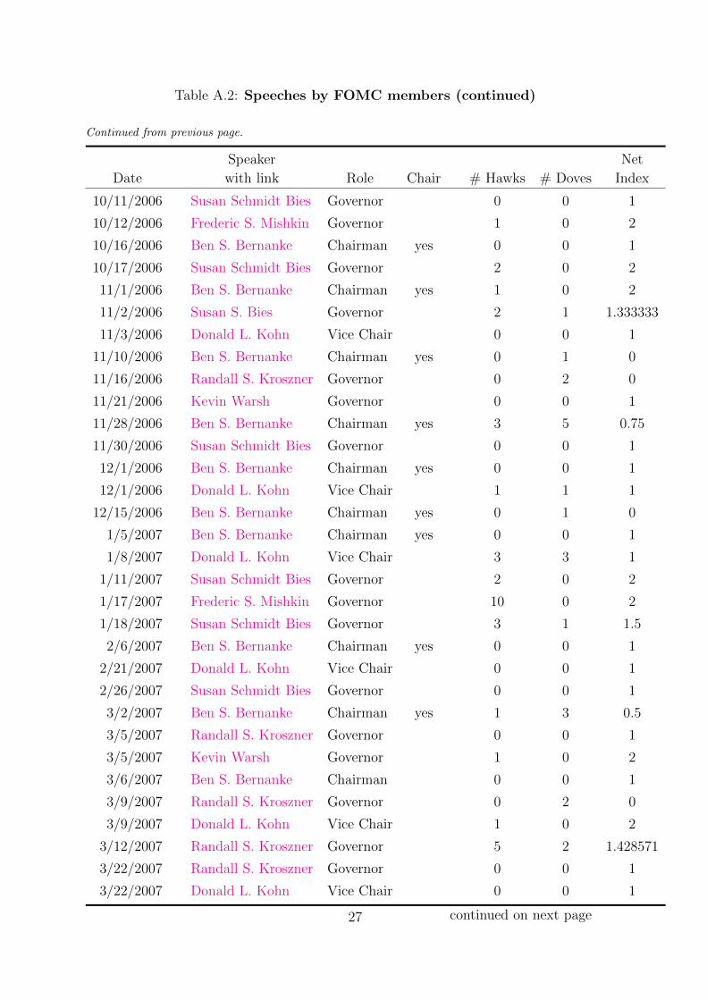
Table A.2: Speeches by FOMC members (continued)
Continued from previous page.
Speaker Net
Date with link Role Chair # Hawks # Doves Index
10/11/2006 Susan Schmidt Bies Governor 0 0 1
10/12/2006 Frederic S. Mishkin Governor 1 0 2
10/16/2006 Ben S. Bernanke Chairman yes 0 0 1
10/17/2006 Susan Schmidt Bies Governor 2 0 2
11/1/2006 Ben S. Bernanke Chairman yes 1 0 2
11/2/2006 Susan S. Bies Governor 2 1 1.333333
11/3/2006 Donald L. Kohn Vice Chair 0 0 1
11/10/2006 Ben S. Bernanke Chairman yes 0 1 0
11/16/2006 Randall S. Kroszner Governor 0 2 0
11/21/2006 Kevin Warsh Governor 0 0 1
11/28/2006 Ben S. Bernanke Chairman yes 3 5 0.75
11/30/2006 Susan Schmidt Bies Governor 0 0 1
12/1/2006 Ben S. Bernanke Chairman yes 0 0 1
12/1/2006 Donald L. Kohn Vice Chair 1 1 1
12/15/2006 Ben S. Bernanke Chairman yes 0 1 0
1/5/2007 Ben S. Bernanke Chairman yes 0 0 1
1/8/2007 Donald L. Kohn Vice Chair 3 3 1
1/11/2007 Susan Schmidt Bies Governor 2 0 2
1/17/2007 Frederic S. Mishkin Governor 10 0 2
1/18/2007 Susan Schmidt Bies Governor 3 1 1.5
2/6/2007 Ben S. Bernanke Chairman yes 0 0 1
2/21/2007 Donald L. Kohn Vice Chair 0 0 1
2/26/2007 Susan Schmidt Bies Governor 0 0 1
3/2/2007 Ben S. Bernanke Chairman yes 1 3 0.5
3/5/2007 Randall S. Kroszner Governor 0 0 1
3/5/2007 Kevin Warsh Governor 1 0 2
3/6/2007 Ben S. Bernanke Chairman 0 0 1
3/9/2007 Randall S. Kroszner Governor 0 2 0
3/9/2007 Donald L. Kohn Vice Chair 1 0 2
3/12/2007 Randall S. Kroszner Governor 5 2 1.428571
3/22/2007 Randall S. Kroszner Governor 0 0 1
3/22/2007 Donald L. Kohn Vice Chair 0 0 1
continued on next page27

Table A.2: Speeches by FOMC members (continued)
Continued from previous page.
Speaker Net
Date with link Role Chair # Hawks # Doves Index
3/23/2007 Frederic S. Mishkin Governor 0 7 0
3/30/2007 Ben S. Bernanke Chairman yes 0 1 0
4/10/2007 Frederic S. Mishkin Governor 3 11 0.428571
4/11/2007 Ben S. Bernanke Chairman yes 0 0 1
4/20/2007 Frederic S. Mishkin Governor 2 2 1
4/25/2007 Ben S. Bernanke Chairman yes 0 0 1
4/26/2007 Frederic S. Mishkin Governor 0 0 1
5/1/2007 Ben S. Bernanke Chairman yes 1 0 2
5/10/2007 Randall S. Kroszner Governor 0 0 1
5/15/2007 Ben S. Bernanke Chairman yes 0 0 1
5/15/2007 Randall S. Kroszner Governor 0 0 1
5/16/2007 Donald L. Kohn Vice Chair 0 0 1
5/16/2007 Randall S. Kroszner Governor 1 1 1
5/17/2007 Ben S. Bernanke Chairman yes 1 0 2
5/22/2007 Ben S. Bernanke Chairman yes 0 0 1
5/23/2007 Randall S. Kroszner Governor 0 0 1
5/24/2007 Frederic S. Mishkin Governor 1 3 0.5
6/1/2007 Randall S. Kroszner Governor 5 1 1.666667
6/5/2007 Ben S. Bernanke Chairman yes 1 0 2
6/5/2007 Kevin Warsh Governor 0 0 1
6/14/2007 Randall S. Kroszner Governor 0 0 1
6/15/2007 Ben S. Bernanke Chairman yes 2 0 2
6/23/2007 Frederic S. Mishkin Governor 0 0 1
7/10/2007 Ben S. Bernanke Chairman yes 4 8 0.666667
7/12/2007 Randall S. Kroszner Governor 0 0 1
8/1/2007 Randall S. Kroszner Governor 0 0 1
8/31/2007 Ben S. Bernanke Chairman yes 2 1 1.333333
9/1/2007 Frederic S. Mishkin Governor 0 1 0
9/6/2007 Randall S. Kroszner Governor 0 0 1
9/10/2007 Frederic S. Mishkin Governor 0 1 0
9/11/2007 Ben S. Bernanke Chairman yes 2 0 2
9/21/2007 Donald L. Kohn Vice Chair 1 4 0.4
continued on next page28

Table A.2: Speeches by FOMC members (continued)
Continued from previous page.
Speaker Net
Date with link Role Chair # Hawks # Doves Index
9/21/2007 Kevin Warsh Governor 0 1 0
9/21/2007 Frederic S. Mishkin Governor 0 0 1
9/24/2007 Ben S. Bernanke Chairman yes 0 0 1
9/27/2007 Frederic S. Mishkin Governor 2 4 0.666667
9/28/2007 Frederic S. Mishkin Governor 1 1 1
10/5/2007 Donald L. Kohn Vice Chair 1 0 2
10/5/2007 Kevin Warsh Governor 0 1 0
10/11/2007 Randall S. Kroszner Governor 0 2 0
10/12/2007 Ben S. Bernanke Chairman yes 0 0 1
10/12/2007 Donald L. Kohn Vice Chair 0 2 0
10/15/2007 Ben S. Bernanke Chairman yes 1 1 1
10/19/2007 Ben S. Bernanke Chairman yes 0 1 0
10/20/2007 Frederic S. Mishkin Governor 7 2 1.555556
10/22/2007 Randall S. Kroszner Governor 0 0 1
10/26/2007 Frederic S. Mishkin Governor 10 4 1.428571
11/5/2007 Frederic S. Mishkin Governor 4 4 1
11/5/2007 Randall S. Kroszner Governor 0 0 1
11/6/2007 Ben S. Bernanke Chairman yes 0 0 1
11/7/2007 Kevin Warsh Governor 0 3 0
11/13/2007 Randall S. Kroszner Governor 0 0 1
11/14/2007 Ben S. Bernanke Chairman yes 0 1 0
11/16/2007 Randall S. Kroszner Governor 2 3 0.8
11/28/2007 Donald L. Kohn Vice Chair 1 2 0.666667
11/29/2007 Ben S. Bernanke Chairman yes 0 0 1
11/29/2007 Frederic S. Mishkin Governor 2 6 0.5
11/30/2007 Randall S. Kroszner Governor 0 0 1
29