monte carlo
TRANSCRIPT

Parallel American Monte Carlo
Calypso Herrera∗ and Louis Paulot†
Misys‡
February 2014
Abstract
In this paper we introduce a new algorithm for American Monte Carlothat can be used either for American-style options, callable structured prod-ucts or for computing counterparty credit risk (e.g. CVA or PFE compu-tation). Leveraging least squares regressions, the main novel feature of ouralgorithm is that it can be fully parallelized. Moreover, there is no needto store the paths and the payoff computation can be done forwards: thisallows to price structured products with complex path and exercise depen-dencies. The key idea of our algorithm is to split the set of paths in severalsubsets which are used iteratively. We give the convergence rate of the algo-rithm. We illustrate our method on an American put option and comparethe results with the Longstaff-Schwartz algorithm.
1 Introduction
American-style derivatives are found in all major financial markets. Monte Carlosimulation is used instead of the finite difference method when the products havemore than two risk factors or have path dependencies.
American Monte Carlo is also important in the context of CVA and PFE com-putations, where conditional expected values have to be computed at differenttimes on simulation paths (Cesari et al., 2009).
The main disadvantage of Monte Carlo simulation is the computation timewhich is significantly higher than for a finite difference or trinomial method. Thisproblem can easily be solved for European-style derivatives: both path genera-tion and payoff computation can be parallelized and only the sum needs to beaggregated at the end. But this is not as simple for American options, callablestructured products or CVA and PFE computations.
∗Quantitative Analyst, [email protected]†Head of Quantitative Research, Sophis, [email protected]‡Sophis Quantitative Research, 42-44 rue Washington, 75008 Paris, France
1
arX
iv:1
404.
1180
v1 [
q-fi
n.C
P] 4
Apr
201
4

The algorithm which is mainly adopted for its simplicity and its robustnessis the Least Squares Monte Carlo (LSM) developed by Longstaff and Schwartz(2001). The American option is approximated by a Bermudan option. Startingfrom the final maturity, at each exercise date one compares the payoff from imme-diate exercise and the expected discounted payoff from continuation. Comparingthe two values, one makes the decision to exercise or to hold the option. Theconditional expectation is estimated from the information of all paths using a leastsquares regression. However, this LSM algorithm with a backward recursion forapproximating the price and the optimal exercise policy cannot be fully paral-lelized. Indeed, at each exercise date, the regression of the continuation value usesinformation from all paths, whose only generation can be parallelized. Howeverand as opposed to European-style options, all paths must be kept in memory andsent to a single computation unit: once the paths are assembled, the least squaresregressions, the optimal exercise decisions and the payoff estimation must be doneby backward recursion.
In this article we address this bottleneck by introducing a new algorithm forAmerican Monte Carlo that can be fully parallelized and relies on least squaresregression to determine the optimal exercise strategy like LSM algorithm.
Our algorithm has several interesting features. Firstly, all the steps of thecomputation can be parallelized. Secondly, there is no need to keep the paths inmemory or transfer them when the computation is done on a grid. Thirdly, oneach path the exercise decision and the payoff computation can be performed for-wards. This allows complex path dependencies, including dependency on exercisedecisions. Fourthly, the algorithm allows the use of a technique known as boost-ing in machine learning in order to get a more precise estimation of the exerciseboundary.
The basic idea is the following. Instead of simulating all paths in a first phaseand perform a backward recursion on all paths together, the set of paths is splitin several subsets which are used iteratively. At each iteration, the coefficientsof the regression are estimated using the paths of the previous iterations. A keyobservation is that in the equation of the least square regression, the informationneeded to compute regression coefficients is encoded in two objects which are linearin the paths (a matrix and a vector). Therefore they can be accumulated on pathsof successive iterations without keeping all paths in memory. Only the linearsystem inversion has to be done at the beginning at each iteration, which can alsobe parallelized.
We prove the convergence of the price and compute the asymptotic error, orequivalently the convergence rate.
We finally illustrate our method with the computation of an American putoption on a single factor. We compare the results and the computation performancewith the LSM algorithm.
Early contributions to the pricing of American options by simulation were madein Bossaerts (1989) and Tilley (1993). Other important works include Barraquandand Martineau (1995), Raymar and Zwecher (1997), Broadie and Glasserman
2

(1997), Broadie and Glasserman (2004), Broadie et al. (1997), Ibanez and Zap-atero (2004) and Garcıa (2000). The idea of computing the expectation value ofcontinuation using a regression was developed by Carriere (1996), Tsitsiklis andVan Roy (2001) and Longstaff and Schwartz (2001).
Several recent articles propose the parallelization of the American option pricinginclude Toke and Girard (2006) and Doan et al. (2010). These articles are basedon the stratification or parametrization techniques to approximate the transitionaldensity function or the early exercise boundary of Ibanez and Zapatero (2004) andPicazo (2002). Recent articles which address partial parallelization of the LSMalgorithm include Choudhury et al. (2008) and Abbas-Turki and Lapeyre (2009).Unlike these articles which study the parallelization of the different phases of theLSM algorithm (path simulation, regression and pricing), we do not parallelizedifferent phases of the LSM algorithm but we propose an innovative algorithmwhich can be fully parallelized.
Convergence of the LSM algorithm was addressed in several articles includingClement et al. (2002) and Stentoft (2004).
Section 2 presents the Longstaff-Schwartz algorithm, including the least squaresregression. Section 3 describes our new algorithm. Section 4 provides numericalresults on the pricing of a put option. Section 5 summarizes the results. Proofs,in particular the convergence rate, are presented in appendices.
2 Longstaff-Schwartz Algorithm
An American-style derivative gives the possibility to the holder to exercise it beforematurity. The holder can choose at any time until the maturity to exercise theoption or to keep it and exercise it later. Bermudan options are similar but exercisecan happen only on specific dates. In order to price them, the American optionsare approximated by Bermudan options with discrete exercise dates. We considerthat the state of the system is described by a vector of state variables Xt. In thesimplest case, it is the spot value of the underlying asset. We assume that thereexists a risk-neutral probability.
2.1 Notations
We denote by t0 the current date. Let us consider an option of maturity T and Nearly exercise dates.
We will use the following notations:
• T maturity of the option
• t0 computation date
• t0 < t1 < ... < tM−1 < tM = T discretized exercise dates
• Xt vector of state variables
3

• Xk = Xtk value of the state variable vector at date tk
• Ck = Ck(Xk) continuation value at date tk
• Ck = Ck(Xk) approximation of the continuation value at date tk
• Fk = Fk(Xk) payoff value in case of exercise at date tk
• Pk = Pk(Xk) discounted value of the option, with optimal exercise at date tkor later.
• rt instantaneous interest rate at time t
2.2 Least squares regression
The American option can be valued using the following recursion. At option ma-turity, the value of the option is equal to the payoff value PM = FM . At a previousdate tk the holder has two possibilities:
• exercise the option and get the cashflow Fk;
• keep the option at least until the next exercise time tk+1. If we assume there isno arbitrage opportunity, the continuation value of the option is the expecteddiscounted value of the option, conditionally to the information available attime tk:
Ck = E(e−
∫ tk+1tk
rsdsPk+1
∣∣∣Xk
). (1)
The holder will exercise if the payoff Fk is higher than the continuation value Ck.Therefore, at time tk the discounted optimally exercised payoff is
Pk =
{Fk Fk ≥ Ck
e−∫ tk+1tk
rsdsPk+1 Fk < Ck .
In a Monte Carlo computation, the conditional value in (1) is not triviallyavailable. One way to estimate it is to approximate it as a linear combination ofbasis functions1:
Ck(Xk) = E(Pk+1
∣∣Xk
)' Ck(Xk) =
p∑l=1
αk,lfk,l(Xk) (2)
with
Pk+1 = e−∫ tk+1tk
rsdsPk+1 .
1This finite linear expansion can be seen as the projection of the infinite-dimensional func-tional space on a finite-dimensional subspace, or equivalently as the truncation of a linear ex-pansion on an infinite number of Hilbert basis functions. There are several choices of the basisfunctions, giving different qualities of approximation.
4

Coefficients αk,l in (2) are estimated using the least squares method. In otherwords, they are chosen to minimize a quadratic error function. Denoting by αk thevector of coefficients, for each date tk we want to minimize
Ψk(αk) = E
wk(Xk)
(Ck −
p∑l=1
αk,lfk,l(Xk)
)2 .
where wk(Xk) are weights which allow to give a different weight to each path. Thechoice of Longstaff and Schwartz is to take the weight equal to 1 when the optionis in the money at time tk and 0 otherwise.
Ck is the conditional expected value E(Pk+1
∣∣Xk
)and is not known, as it is
the function we want to estimate. Therefore the least square regression cannot bedirectly applied. However, minimizing Ψk is equivalent to minimizing a differentfunction:
Φk(αk) = E
[wk(Xk)
(Pk+1 −
p∑l=1
αk,lfk,l(Xk)
)2]
.
See appendix A for a proof. The difference between Φk and Ψk is that there areno more conditional expectations. Thus the coefficients of the basis functions canbe estimated using the least square method, by regressing the discounted optionvalues Pk+1 on the state variable values Xk at tk.
In practice, the expected value in Φk which is minimized is, up to an irrelevantfactor N , the Monte Carlo estimation
Φk(αk,l) =N∑j=1
wk
(X
(j)k
)(P
(j)k+1 −
p∑l=1
αk,lfk,l
(X
(j)k
))2
where X(j)k is the state variable vector on path j at time tk and P
(j)k+1 is the value
of the stochastic variable Pk+1 on path j. The weights wk
(X
(j)k
)allow to focus on
the more relevant paths, as explained in section 3.6.This function Φk has a minimum on αk when the partial derivative with respect
to αk,l are zero for all l:
∂Φk
∂αk,l= 2
p∑m=1
N∑j=1
wk
(X
(j)k
)fk,l
(X
(j)k
)fk,m
(X
(j)k
)αk,m
− 2N∑j=1
wk
(X
(j)k
)fk,l
(X
(j)k
)P
(j)k+1 = 0 . (3)
Let us introduce p× p matrix Uk and dimension p vector Vk
Uk,lm =N∑j=1
wk
(X
(j)k
)fk,l
(X
(j)k
)fk,m
(X
(j)k
)Vk,l =
N∑j=1
wk
(X
(j)k
)fk,l
(X
(j)k
)P
(j)k+1
5

or in a simpler, vectorial notation
Uk =N∑j=1
wk
(X
(j)k
)fk
(X
(j)k
)f>k
(X
(j)k
)Vk =
N∑j=1
wk
(X
(j)k
)fk
(X
(j)k
)P
(j)k+1 . (4)
We can rewrite equation (3) asUkαk = Vk .
For each date tk coefficients αk are therefore obtained through matrix inversion orusing a linear equation solver:
αk = U−1k Vk .
This is the vector of coefficients which minimizes the quadratic error function. Itgives the least square estimation of the continuation value of the option at time tkon N Monte Carlo paths:
Ck(Xk) =
p∑l=1
αk,lfk,l(Xk) = α>k fk(Xk) .
When the coefficients are estimated, they are used to compute the continuationvalue at time tk for each path. The continuation value will be used for the decisionto continue or to exercise the option. When the decision is made, we have thecashflow at time tk. If the decision is to continue, we use the simulated value ofthe payoff and not the estimated value. For each path, we compute the cashflowfor all dates backwards.
2.3 Algorithm
In summary, the Longstaff-Schwartz algorithm is the following:
1. Simulate N Monte Carlo paths X(j)k (1 ≤ j ≤ N , 1 ≤ k ≤M) and keep them
in memory or store them.
2. On the last date tM , compute the terminal payoff P(j)M = FM
(X
(j)N
)on all
paths j.
3. Starting from k = M − 1 and until k = 1, perform a backward recursion:
(a) Summing over all paths and using payoff value at date tk+1, compute
Uk =N∑j=1
wk
(X
(j)k
)fk
(X
(j)k
)f>k
(X
(j)k
)Vk =
N∑j=1
wk
(X
(j)k
)fk
(X
(j)k
)P
(j)k+1 .
6

(b) Get least square coefficients αk = U−1k Vk .
(c) On every path j, compare the payoff value Fk
(X
(j)k
)and the continua-
tion value estimate Ck
(X
(j)k
)= α>k fk
(X
(j)k
). If Fk
(X
(j)k
)≥ Ck
(X
(j)k
),
set P(j)k = Fk
(X
(j)k
); else set P
(j)k = P
(j)k+1 = e−
∫ tk+1tk
rsdsP(j)k+1.
4. Finally get the Monte Carlo estimate of the derivative price as
P =1
N
N∑j=1
P(j)1 . (5)
2.4 Limitations
The Longstaff-Schwarz algorithm is powerful and allows to price multi-factor, path-dependent derivatives with early exercise using Monte Carlo simulations. However,we can state a few limitations
Parallelization Monte Carlo pricing is time-consuming. In order to get good per-formance, we want to parallelize the computations. In the standard AmericanMonte Carlo algorithms, such as the Longstaff-Schwartz algorithm that wedescribed, only the path generation can be parallelized. Since it makes useof all paths, the backward regression has to be done on a single computationunit. This includes the least square estimation of the continuation value, theexercise decision and the computation of P
(j)k on each path.
Memory consumption Since all paths must be generated in a first phase andused in a second one, all paths must be stored. For an option with severalunderlyings and many exercise dates, this can represent large amounts ofdata. In addition, if the path generation is distributed on some grid, itmeans that a large quantity of data must be transferred.
Limited path dependence As the payoff is computed backwards, the path de-pendence is limited to quantities present in the state variables vector. Itcan include quantities which depend on past values on a given path but notquantities which depend on exercise decisions at previous dates.
As an example, a swing option allows to buy some asset (usually electricityor gas) at several dates for a price fixed in the contract, with some globalminimum and maximum on the total quantity. This means that exercising ondate tk depends on the exercises on date tk′ , k
′ < k. This cannot be directlyhandled by a standard Longstaff-Schwartz algorithm.
3 Parallel iterative algorithm
We propose an algorithm for American Monte Carlo with the following properties.
7

Full parallelization All phases of the computation can be parallelized.
No path storage Monte Carlo paths are used only once. There is no need tokeep them in memory or transfer them when the computation is done on agrid. Only fewer aggregated data are kept in memory and exchanged betweencomputation units.
Forward computation On every path, exercise decisions and payoff computa-tion can be performed forwards from t1 to tM . This allows all kinds ofpath-dependence, including dependence on previous exercise decisions.
Boosting The algorithm allows to use some boosting in order to get more andmore precise estimates of the exercise boundaries.
More general regression Least square regression can be performed for all orseveral dates together, introducing exercise time as a variable of the contin-uation value function.
3.1 Iterations
Instead of simulating all paths in a first step and performing a backward recursionon all paths together in a second step, the N paths are split in several sets whichare used iteratively. On each iteration, coefficients αk are estimated using pathsof the previous iterations. A key observation is that in equation (4) Uk and Vk arelinear in the paths. The information needed to compute regression coefficients isencoded in these objects and can be accumulated on paths and successive iterationswithout keeping all paths in memory. Only the linear system inversion has to bedone at the beginning of each iteration.
For a given iteration, the exercise decisions depend on objects Uk and Vk ob-tained in previous iterations. Within this iteration, computations on differentpaths are independent from each other. This means that they can be run in par-allel. Once quantities from all paths in a given iteration are accumulated, solvingthe linear system can be done independently for every date. Therefore this canalso be parallelized.
In addition, as the exercise decision is made using information from previousiterations, there is no need to use a backward computation: all payoff computationsand exercise decisions can be done in the natural order. (Note that in simple cases,it may however require less calculations to do it backwards on a given path.)
One may think that using only a limited number of paths to make the exercisedecisions in the first iterations will increase the error in the final price. Howeverit appears that this effect is small after a few iterations. In order to reduce theerror in the final results, we introduce weights depending on the iteration in bothformulas (4) and (5): paths from first iterations are less weighted than paths fromthe following iterations which are more precise.
In fact, the iterative nature of our algorithm even allows to use somethingsimilar to what is called boosting in machine learning, as already introduced in the
8

context of American options pricing in Picazo (2002). This can eventually givesmaller errors than classical Longstaff-Schwartz algorithm.
3.2 Notations
The N paths are partitioned in n distinct sets. Let us assume each piece of thepartition is made of consecutive paths and denote by ni, 1 ≤ i ≤ n the final pathof each set. This means that the ith iteration will use paths from ni−1 + 1 to ni.
• M : number of exercise dates.
• N : total number of paths.
• n: number of iterations.
• ni: last path of ith iteration. Iteration i uses path ni−1 +1 to ni, with n0 = 0and nn = N .
• wi: weight of paths of the ith iteration in the price sum.
• w(i)k
(X
(j)k
): weight of path j inside iteration i in matrix U and vector V sums
in equations (4). A special case is the factorization w(i)k (Xk) = wiyk(Xk).
• U(i)k and V
(i)k : matrices and vectors containing information from path 1 to ni
and used to compute α(i)k .
• u(i)k and v
(i)k : contributions of iteration i to U
(i)k and V
(i)k , containing informa-
tion from paths ni−1 + 1 o ni.
• α(i)k : vector of coefficients regressed on paths 1 to ni.
• C(i)k (Xk): approximated continuation value given by coefficients α
(i)k . It is
used in iteration i+ 1.
• κ(j)k : optimal exercise time index κ, such that optimal exercise time is tκ on
path j if not exercised before tk.
• P(j)k : discounted payoff on path j at time tk if the option is not exercised
before.
• P (i): sum of option discounted payoff from paths of the ith iteration.
• PN : total weighted sum of discounted option payoff from paths 1 to N.
• qN : sum of price weights of paths 1 to N.
9

3.3 Algorithm
1. Initiate the algorithm using rough estimates for exercise boundaries or coeffi-cients α
(0)k : for example consider that the option is exercised at final maturity
only or, alternatively, use final coefficients from previous day computation.
2. Iterate on i from 1 to n:
(a) Iterate on j from ni−1 + 1 to ni:
i. Simulate path j and get state variable vector X(j)k at all dates.
ii. For all dates tk, compare the payoff value Fk
(X
(j)k
)and the continuation
value estimate from the previous iteration
C(i−1)k
(X
(j)k
)= α
(i−1)>k fk
(X
(j)k
).
From this, for all k get2
κ(j)k = min
(k′ ≥ k
∣∣∣∣ k′ = N or Fk′(X
(j)k′
)≥ C
(i−1)k′
(X
(j)k′
))
and finally P(j)k = e−
∫ κ(j)k
tkrsdsF
κ(j)k
(X
(j)
κ(j)k
)and P
(j)k+1 = e−
∫ tk+1tk
rsdsP(j)k+1.
iii. Accumulate the contribution to the price
P (i) =
ni∑j=ni−1+1
P(j)1 .
iv. For every date tk add the contribution of path j to
u(i)k =
ni∑j=ni−1+1
w(i)k
(X
(j)k
)fk
(X
(j)k
)f>k
(X
(j)k
)v
(i)k =
ni∑j=ni−1+1
w(i)k
(X
(j)k
)fk
(X
(j)k
)P
(j)k+1 .
2This computation can be done in a forward manner, however numerically, the fastest wayto perform this computation is to do it backwards. Starting on the last exercise date tM we set
P(j)M = FM
(X
(j)M
). Then recursively on k, if Fk
(X
(j)k
)≥ C
(i−1)k
(X
(j)k
), set P
(j)k = Fk
(X
(j)k
);
else set P(j)k = P
(j)k+1 = e−
∫ tk+1tk
rsdsP(j)k+1.
10

(b) For every date tk, add the contributions u(i)k and v
(i)k of iteration i to3
U(i)k =
i∑l=1
u(l)k
V(i)k =
i∑l=1
v(l)k ,
solve the linear systemU
(i)k α
(i)k = V
(i)k
and get the coefficients of the least squares regression on ni first paths:
α(i)k =
(U
(i)k
)−1
V(i)k .
(c) Using price weights wi, accumulate the contributions of iteration i to
PN =n∑i=1
wiP(i)
qN =n∑i=1
wi(ni − ni−1) .
3. Finally get the Monte Carlo estimate of the option price as the weightedaverage
P =PNqN
.
3.4 Parallel computing
For every iteration, steps (a) and (b) can inherently be parallelized. In step (a), allthe paths in a given iteration are independent from each other and computationrelated to different paths can be run in parallel. Similarly, the linear systems fordifferent dates in (b) can be solved in parallel.
The data which must be shared or transfered between computation units areobjects Uk and Vk for all dates, coefficients αk and contribution to the final priceP (i).
3When the weight w(i)k (Xk) factorizes as w
(i)k (Xk) = wiyk(Xk), the multiplication by wi can
be factorized at this step: u(i)k =
∑ni
j=ni−1+1 yk
(X
(j)k
)fk
(X
(j)k
)f>k
(X
(j)k
)and U
(i)k = U
(i−1)k +
wiu(i)k and similarly for V .
11

3.5 Convergence
We assume weights wi ∼ 1 when i→∞. We also assume that w(i)k (Xk) factorizes
as w(i)k (Xk) = wiyk(Xk) with wi ∼ 1 when i→∞.
Let us fix a vector of initial regression coefficients α. Using these coefficientsin exercise decisions, let us define u(α) = E
[f(X)f(X)>
]and v(α) = E
[f(X)P
].
This gives a function α 7→ α(α) = u(α)−1v(α). This corresponds to the vectorof coefficients obtained after a single iteration in the limit of an infinite numberof paths. Let us assume this function α 7→ α(α) is contractant, i.e. Lipschitz-continuous
∀α, α′ ‖α(α)− α(α′)‖ ≤ q‖α− α′‖
with4 q < 1.The Banach fixed-point theorem then ensures this function has a fixed point.
Let us denote by A the norm of the (matrix) operator ∂α(α)∂α
at this fixed point. Wehave A ≤ q < 1.
Let us assume there are n iterations of m paths, with a total number of pathsN = nm.
Then the algorithm we propose converges to an approximation of the price asn→∞.
As the continuation value is projected on a finite dimensional basis, exerciseboundaries are approximations and therefore the exercise is slightly sub-optimal.As a consequence, the algorithm converges to a value which is lower than the realprice. When the number of basis functions grows, the price estimate becomes closerto the real price. The same behavior is observed in Lonstaff-Schwartz algorithm.The error term around this limit value has an expected value in O
(1
n1−A
)and a
standard error in O(
1√mnmax(1,2−2A)
). If A ≤ 1
2, this is the usual Monte Carlo error
O(
1√nm
)= O
(1√N
).
When the weights of the paths in yk(Xk) are the same as chosen by Longstaff
and Schwartz, 1 in the money and 0 out of the money, then the algorithm convergesto the same price as Longstaff-Schwartz algorithm.
The proof is given in appendix B.
3.6 Path weights
In order to improve the convergence of the algorithm, the paths can be givendifferent weights, in the computation of matrix U and vector V on one hand, andin the price computation on the other hand.
4For an American option, the continuation value for a given date reaches a maximum whenthe estimated continuation value is exact for the following dates. As a consequence, ∂α∂α vanishesfor the optimal α. Around this point, it is not a strong constraint to assume that the function iscontractant.
12

3.6.1 Exercise boundary
Longstaff and Schwartz use a simple weight for paths in the regression: at datetk, path j is taken into account only if the option is in the money at date tk. Theweight wk(X
(j)k ) is equal to 1 when the option is in the money and 0 otherwise.
This is used for the computation of the matrix Uk and the vector Vk in the equation(4). This weight improve the convergence of the algorithm: the paths in the moneyare the only paths eligible to be exercised.
Going further, we want to concentrate on paths which are closed to the exerciseboundary. In addition, we require the weight to be continuous, which will givesmoother greeks.
In the case of a product on one underlying, we suggest a simple weight function:
yk(Xk) = e− (Xk−Bk)2
2β2k
where Xk is the spot price at the date tk and Bk is the exercise boundary valueat the same date. At each date tk, the exercise boundary is the solution of theequation Fk(x) = Ck(x) where Fk is the payoff value and Ck is the continuationvalue estimate. The boundary is computed using the coefficients αk of the previousiteration. This equation can be approximatively solved with a simple numericalmethod.
Parameters βk are chosen to give a good compromise between statistical errorand systematic error. The statistical error is reduced for large βk, when many pathsare taken into account. The systematic error is reduced when we only look at pathsclose to the exercise boundary, for small βk. We can use the iterative nature ofour algorithm to reduce βk as the number of iterations grows. This would allowboth statistical and systematic error to be reduced. This is similar to boostingin machine learning: as the number of iterations increases, we concentrate moreclosely around the exercise boundary.
3.6.2 Iterations and weights on U ,V
As the algorithm is iterative, the values of the regression coefficients are not precisein the first iterations. For this reason, a simple optimization of the algorithm isto give a low weight to the first iterations. At each iteration, the matrix U
(i)k
and the vector V(i)k are filled and added to the U
(i−1)k and V
(i−1)k of the previous
iteration. We introduce a weight which increases with the number of iteration i:wi =
∏nj=i+1w
(i)UV with
w(i)UV = 1− λe−
iµ . (6)
Each U(i)k and V
(i)k from previous iteration are multiplied by w
(i)UV . This decreases
the weight of first iterations in the regression coefficients.
13

3.6.3 Iterations and weights on price
Similarly, during the first iterations the estimated continuation value is not accurateas the coefficients αk are not and therefore neither the price. A simple way toimprove the convergence is to eliminate the first paths from the computation ofthe final price. For this reason the final price is a weighted average where the firstpaths do not have an important weight. We introduce a weight wi which dependson the iteration. The weight increases with the iterations.
We use the following function:
wi = 1− 1
2(1− tanh [ν(i− 1)]) . (7)
At each iteration i, we multiply the sum of present values of iteration i by thisweight wi before adding to the sum of present values of the previous iterations.
3.7 Time as a variable of regression functions
Finally one can leverage the iterative nature of our algorithm to lower the totalnumber of basis functions in the regression and decrease the statistical error of theleast squares estimation.
In the simplest algorithm, the regression is made independently for each date:for each date tk, we compute the matrix Uk and the vector Vk, we solve the equa-tion Ukαk = Vk in order to obtain the vector of coefficients αk. It is possible toavoid making a regression at each date, by including the time in the regression.Discounted cash flows Pk+1 are regressed against the state variable vector Xk andagainst the time tk. This means that the basis functions include the time tk as avariable. fk,l(Xk) is generalized to fl(X, t):
C(j)k ' Ck
(X
(j)k
)=
p∑l=1
αlfl(X(j)k , tk)
In this general case, we minimize the error function
Ψ(α) =M∑k=1
E
[wk(Xk)
(Ck −
p∑l=1
αlfl(Xk, tk)
)2]
.
Similarly to what is explained is section 2.2 we build a p×p matrix and a dimensionp vector
U =N∑j=1
M∑k=1
wk
(X
(j)k
)f(X
(j)k
)f>(X
(j)k
)V =
N∑j=1
M∑k=1
wk
(X
(j)k
)f(X
(j)k
)P
(j)k+1 . (8)
14
Then we solve the linear equation Uα = V and get least squares coefficients α =U−1V .
When the number of basis function is large, solving the linear system can betime-consuming if matrix U is dense. However we can choose basis functions sothat U is block-diagonal. This is obtained if basis functions are divided in subsetswith disjoint supports. To be more precise, let us assume we have B blocks, labeled
by b. We denote by pb the number of basis functions in block b, withB∑b=1
pb = p.
Inside block b, we denote basis functions by fb,l with 1 ≤ l ≤ pb. Functions whichbelong to two different blocks have disjoint support on (X, t). Therefore, if b 6= b′
for all X and t we have fb,l(X, t)fb′,l′(X, t) = 0. From the definition of matrix Uin equations (8) this means U is block-diagonal. We denote by fb the vector ofbasis functions in block b, Ub the diagonal blocks of matrix U , with a similar splitof vector V in Vb:
Ub =N∑j=1
M∑k=1
wk
(X
(j)k
)fb
(X
(j)k
)f>b
(X
(j)k
)Vb =
N∑j=1
M∑k=1
wk
(X
(j)k
)fb
(X
(j)k
)P
(j)k+1 .
The classical date by date regression is the special case where a block corre-sponds to a given exercise date and where basis function are fb,l(X, t) = fb,l(X)1t=tb .
An other possibility, which requires fewer basis functions, is to partition thetotal set of exercise dates in B groups of consecutive dates, with basis functionsof a given block concentrated on the corresponding dates and null for other dates.If block b corresponds to exercise dates tk with kb−1 < k ≤ kb, basis functions aretaken of the form fb,l(X, t) = fb,l(X, t)1tkb−1<t<tkb
. As an example, if we have a set
of p basis functions fl(X) in the X variable, we can construct a basis of functionswith affine dependence on t with
fb,2l−1(X, t) = fl(X)1tkb−1<t<tkb
fb,2l(X, t) = tfl(X)1tkb−1<t<tkb
Thanks to that, the coefficients αk won’t be computed at all dates. We will haveonly a matrix Ub and the vector Vb for a set of exercise times [tkb−1+1, . . . , tkb ]. Inaddition, this can reduce the statistical error on the exercise boundary: for a givennumber of paths there are more contributions in U and V .
4 Numerical results
We consider the example of an American put on an asset St. Assume that the stockprice follows the Black-Scholes dynamic and that there is no arbitrage opportunity.
15

The risk-neutral process of the stock price is the following:
dSt = rStdt+ σStdWt .
The risk-less interest rate r and the volatility σ are assumed to be constant. Thereare no dividends. We denote by K the strike price and by T the maturity of theoption.
We use the same example as in Longstaff and Schwartz (2001). We price anAmerican put option on a share with strike price $40. The annual interest rateis 6%, the underlying stock price is $36, the volatility σ is 20% and the maturity1 year. We consider that the option can be exercised 50 dates per year until itsmaturity.
We generate 100,000 paths. In the parallel algorithm, we use 100 iterations,independently of the total number of paths. We choose 5 groups of 10 dates. Thebasis functions chosen for the regression are : 1, S, S2, t, tS and tS2. We haveweights on U and V , wUV with λ = 2 and µ = 2. We use weights on prices wi withν = 0.99. We also have the weight depending on the path yk.
We compare results with a reference value of $4.486 given by a finite differencemethod. We use an implicit scheme with 40,000 time steps and 1,000 steps for thestock price.
4.1 Convergence of the algorithm
We have implemented the parallel algorithm and we have compared it with thefinite difference method. We have tested the impact of the number of iterationsand the number of dates per block. The finite difference American is the result ofa the discretization of the Black-Scholes equation:
∂tP +1
2σ2S2∂S2P + rS∂SP − rP = 0
with the terminal condition P (T, S) = max(0, S −K).
4.1.1 Number of iterations
Our example is tested on a quad-core CPU. We parallelize the algorithm on fourthreads. In each thread, the paths are generated and the matrices Ub and vectorsVb are computed for each date k. For each thread, we only need to keep Ub, Vbfor all b and the sum of the present value. When computation is finished in allthreads, the results are aggregated. When we have the global Ub and Vb which arethe sum of all the matrices Ub and vectors Vb of each thread, the coefficients αb ofthe regression are computed by solving Ubαb = Vb. This step is also done in parallelby solving this equation for a block of dates b in each thread. When the coefficientsare computed, we use them in the following iteration for the computation of Ukand Vk and also the option price. In the first iteration we do not have the αk
16

needed. We make the decision to keep the option until its maturity. We could alsouse coefficients from the previous day computation.
Figure 1 shows the impact of the number of iterations on the final price. In thisfigure, the total number of paths generated remains the same, only the number ofpaths per iteration changes.
4
4.1
4.2
4.3
4.4
4.5
0 50 100 150 200
Pric
e
Number of iterations
Confidence IntervalPrice
Figure 1: The impact of the number of iterations for a given number of paths(100,000) on the price.
During the Monte Carlo pricing we compute the (weighted) variance of prices
V = 1qN
∑ni=1 wi
∑nij=ni−1+1 P
(j)1
2− P 2 with qN =
∑ni=1 wi(ni − ni−1). Using also
q(2)N =
∑ni=1 w
2i (ni−ni−1) we get the standard error estimate ε =
√V q
(2)N
q2N
. We plot
the statistical 95% confidence interval, which corresponds to ±1.96ε. Note that ittakes into account statistical error only and not systematic error.
The price converges closer to the real price $4.486 when the number of iterationsincreases. We notice that for 100,000 paths, 100 iterations are sufficient to converge.Going further, figure 2 presents the price convergence for different numbers ofiterations [10, 20, 100, 200]. Similarly, figure 3 shows the convergence of the early-exercise boundary at the mid-maturity date. The convergence is faster for a largernumber of iterations. However the difference between 100 and 200 iterations isnot significant. In these two cases, a good price estimate is obtained after 10,000paths. In addition, we notice that for 100,000 paths, the price obtained with only10 iterations is different from the price with 200 iterations by less than two standarderrors.
17

3.8
3.9
4
4.1
4.2
4.3
4.4
4.5
10000 20000 30000 40000 50000 60000 70000 80000 90000 100000
Pric
e
Number of paths
10 iterations20 iterations
100 iterations200 iterations
Figure 2: The impact of the number of iterations on the American put price.
34.5
35
35.5
36
36.5
10000 20000 30000 40000 50000 60000 70000 80000 90000 100000
Exer
cice
bou
ndar
y
Number of paths
10 iterations20 iterations
100 iterations200 iterations
Figure 3: The impact of the number of iterations on the American put early exerciseboundary at the mid-maturity date.
18

4.1.2 Weights for U, V and price
As the algorithm is iterative, the values of the regressions coefficients and of theprice are not correct for the first iterations. We have added the rescaling factorw
(i)UV from equation (6) with λ = 2 and µ = 2. Each Uk and Vk from previous
iteration are multiplied by w(i)UV .
In the same way, we add a weight on the price that depends on the number ofiteration wi from equation (7) with ν = 0.99. At each iteration i, we multiply thesum of present values of the paths in the iteration by wi before adding to the sumof present values of the previous iterations. In figure 4 we show the impact of thevarious weights on the price. The price converges faster if we add weights in bothU , V and in the price. We also plot an early exercise boundary in figure 5.
4.05
4.1
4.15
4.2
4.25
4.3
4.35
4.4
4.45
4.5
4.55
50000 100000 150000 200000
Pric
e
Number of paths
Without rescalingRescaling price
Rescaling UVRescaling price and UV
Figure 4: The impact of weighting the price or U, V for each iteration on theAmerican put price.
It corresponds to the boundary at the mid-maturity date. One can see thatthe weight of U and V , wi has an impact on the boundary but not the weight ofthe price wi. This is due to the fact that wi has an impact on the coefficients αb ofthe regression which are used in the computation of the exercise boundary. On theopposite, the weight on the price wi does not have an impact on the boundary, asthe rescaling is done on the price alone, after the computation of the coefficientsand exercise boundaries.
19

33.5
34
34.5
35
35.5
36
50000 100000 150000 200000
Exer
cice
bou
ndar
y
Number of paths
Without rescalingRescaling UV
Rescaling priceRescaling price and UV
Figure 5: The impact of weighting the price or U, V for each iteration on theAmerican put early exercise boundary at mid-maturity.
4.1.3 Size of date groups
In the algorithm of Longstaff-Schwartz, a regression is made at each date tk. Wechoose as basis functions 1, S and S2. The continuation value is estimated as
E[P (St+1)|St] ' α + βSt + γS2t .
The coefficients are computed at each time tk in [t1, ..., tM ]. We include the timein the regression variables and we add three more basis functions: t, tS and tS2:
E[P (St+1)|St, t] = α + βSt + γS2t + δt+ εtSt + ζtS2
t .
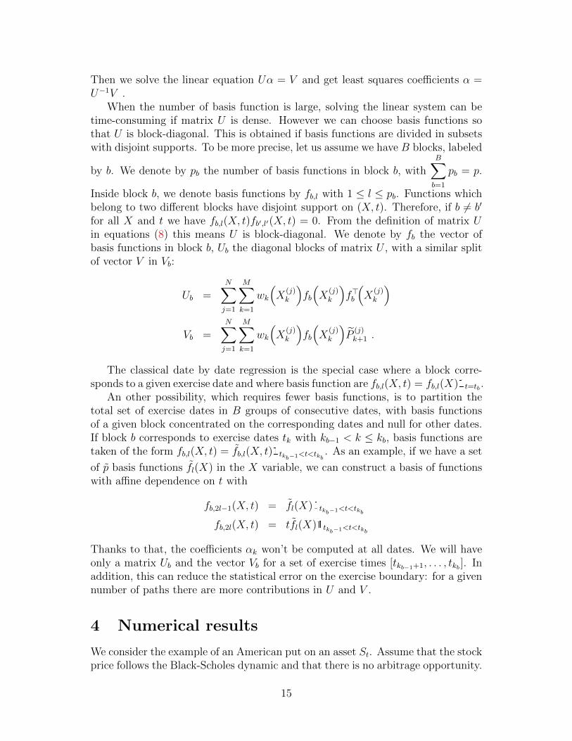
We make groups of D dates [tbD−D+1, ..., tbD]. The resolution of the equationUbαb = Vb is made only once per group of dates. With the coefficients computedfor one group b, we can estimate the discounted value P for all dates within thegroup [tbD−D+1, ..., tbD]. We have tested for several sizes of dates groups. As figure6 shows, the number of dates per group does not have an important impact onthe price. In the graph, we also have the case of one date per group, which meansthat we are in the first case with three basis functions. The price estimate is verysimilar in both cases. With more dates per group, the total number of groups isreduced and thus also the number of linear systems to inverse. Therefore, usinggroups of dates may save some computation time and reduce the quantity of datato transfer without deteriorating the precision of the price.
20
4.4
4.42
4.44
4.46
4.48
4.5
4.52
0 10 20 30 40 50
Pric
e
Number of dates per block
Confidence IntervalPrice
Figure 6: The impact of the size of the dates groups on the American put price.
4.2 Comparison with Longstaff Schwartz
In this section we compare our parallel algorithm with the Longstaff-Schwartzalgorithm, using the same example and parameters. We show the price for differentnumbers of paths in figure 7.
Both algorithms converge to the same price which is below the $4.486 price ob-tained with finite difference method by 1.9¢ (0.4% relative error). As we explainedin section 3.5 this is due to the approximation of the continuation value whichmakes the exercise slightly sub-optimal.
What is remarkable and innovative is that the parallel algorithm is using allavailable threads (in our example, four) during the whole computation. TheLongstaff-Schwartz algorithm uses only one thread. Thus for 100,000 paths theLongstaff-Schwartz needs 14.37 seconds while the parallel algorithm takes only 3.6seconds, as shown in figure 8. One observes a good scaling property. Even ifone parallelizes the path generation step in the LSM, we still have an importantimprovement with our algorithm5. Figure 9 plots the price estimate against thecomputing time for both algorithm in our quad-core example.
In table 1 we compare the price of American put options on a share usingthe Longstaff-Schwartz algorithm, the parallel algorithm and the finite difference
5In our example, path generation takes 8.42 seconds over a total of 14.37 seconds in LSM.Parallelizing this step would give a total computation time of at least 8.05 seconds versus 3.6seconds with our algorithm. This is without taking in consideration the memory issues and thedata transfer cost.
21

4.25
4.3
4.35
4.4
4.45
4.5
4.55
4.6
4.65
0 10000 20000 30000 40000 50000 60000 70000 80000 90000 100000
Pric
e
Number of paths
Parallel AlgorithmLongstaff Schwartz
Finite Difference American
Figure 7: Convergence of Longstaff Schwartz vs Parallel Algorithm.
0
2
4
6
8
10
12
14
16
0 10000 20000 30000 40000 50000 60000 70000 80000 90000 100000
Com
puta
tion
time
in s
econ
ds
Number of paths
Parallel AlgorithmLongstaff Schwartz
Figure 8: Computation time of Longstaff-Schwartz vs Parallel Algorithm with 4cores.
22

4.3
4.35
4.4
4.45
4.5
4.55
4.6
0 2 4 6 8 10 12 14
Pric
e
Computation time in seconds
Parallel AlgorithmLongstaff Schwartz
Finite Difference American
Figure 9: The convergence of the price with respect to the computing time.
method. We use the same parameters as in the previous example. We computethe price for different values of the underlying spot price S = 36, 38, 40, 42, 44, ofthe volatility σ = 20%, 40% and of the maturity T = 1, 2. In this table, we alsopresent the standard error (s.e) for each algorithm, the price of a European putoption and the early exercise value which is the difference between the Americanand the European price.
The differences between the finite difference and the LSM algorithm are verysmall. The 20 differences are less or equal to 2.2¢, among which 9 values are lessor equal to 1¢. The standard error for the simulated value ranges from 0.7¢ to2.2¢. The differences of the finite difference and the parallel algorithm are evensmaller. The 20 differences are less or equal to 1.9¢, among which 16 values are lessor equal to 1¢. The standard errors are similar to the LSM standard errors, 0.6¢ to2.2¢. All differences between the LSM and the parallel algorithm are smaller thanone standard error. The differences with the finite difference are both positive andnegative for both algorithms.
4.3 Improved exercise decision in the first iteration
At each iteration, the exercise strategy is determined by the coefficients comingfrom the previous iterations. In the first iteration, the coefficients are not available.Therefore, for the first iteration, the choice made in our previous examples was toexercise the option at the maturity.
23

Fin
ite
Lea
stP
aral
lel
Par
alle
lC
lose
dE
arly
Ear
lyE
arly
Diff
eren
ceD
iffer
ence
Diff
eren
ceD
iffer
ence
Squar
esL
SA
lgor
ithm
Alg
orit
hm
For
mu
laE
xer
cise
Exer
cise
Exer
cise
PD
Ean
dP
DE
and
LS
and
Sσ
TA
mer
ican
Sim
ula
tion
(s.e
)S
imu
lati
on(s
.e)
Eu
rop
ean
PD
EL
SP
aral
lel
LS
Par
alle
lP
aral
lel
36
0.2
14.4
864.
467
(.00
9)4.
467
(.00
9)3.
844
.642
.622
.623
.019
.019
.000
36
0.2
24.8
474.
833
(.01
1)4.
838
(.01
1)3.
763
1.08
41.
070
1.07
5.0
14.0
09-.
005
36
0.4
17.1
097.
087
(.01
9)7.
100
(.01
9)6.
711
.398
.376
.389
.022
.009
-.01
336
0.4
28.5
138.
512
(.02
2)8.
521
(.02
2)7.
700
.813
.812
.821
.001
-.00
8-.
009
38
0.2
13.2
573.
237
(.00
9)3.
247
(.00
9)2.
852
.405
.385
.395
.020
.009
-.01
138
0.2
23.7
503.
738
(.01
1)3.
753
(.01
1)2.
991
.760
.747
.762
.012
-.00
3-.
015
38
0.4
16.1
556.
145
(.01
9)6.
151
(.01
8)5.
834
.320
.310
.317
.010
.004
-.00
738
0.4
27.6
747.
663
(.02
2)7.
678
(.02
2)6.
979
.696
.684
.699
.011
-.00
3-.
015
40
0.2
12.3
192.
305
(.00
9)2.
306
(.00
8)2.
066
.253
.239
.240
.014
.013
-.00
140
0.2
22.8
892.
870
(.01
1)2.
878
(.01
0)2.
356
.533
.515
.523
.019
.011
-.00
840
0.4
15.3
195.
306
(.01
8)5.
310
(.01
8)5.
060
.259
.247
.251
.012
.008
-.00
440
0.4
26.9
236.
918
(.02
2)6.
924
(.02
1)6.
326
.597
.592
.598
.005
-.00
1-.
006
42
0.2
11.6
211.
615
(.00
8)1.
613
(.00
7)1.
465
.157
.151
.149
.006
.008
.002
42
0.2
22.2
162.
194
(.01
0)2.
204
(.00
9)1.
841
.375
.353
.362
.022
.012
-.01
042
0.4
14.5
894.
591
(.01
7)4.
584
(.01
7)4.
379
.210
.212
.205
-.00
3.0
05.0
0742
0.4
26.2
506.
241
(.02
1)6.
247
(.02
1)5.
736
.514
.506
.511
.009
.003
-.00
6
44
0.2
11.1
131.
112
(.00
7)1.
109
(.00
6)1.
017
.096
.095
.092
.001
.004
.003
44
0.2
21.6
931.
680
(.00
9)1.
686
(.00
9)1.
429
.264
.251
.257
.013
.007
-.00
644
0.4
13.9
533.
959
(.01
6)3.
952
(.01
6)3.
783
.171
.177
.169
-.00
6.0
01.0
0744
0.4
25.6
475.
651
(.02
1)5.
651
(.02
0)5.
202
.445
.449
.449
-.00
4-.
004
.000
Tab
le1:
Com
par
ison
ofth
eA
mer
ican
put
pri
ces.
24

Another solution is to use the coefficients of the previous computation, whichis usually made the previous day. We illustrate this case in the figures 10, 11 and12.
In this example for the first iteration only we use the coefficients and thereforethe exercise boundaries computed in a previous computation, with different marketparameters. The interest rate is 5.5%, the volatility σ is 22% and the spot valueis $34.
Figure 10 shows the convergence of the put price. We launch several times
4.25
4.3
4.35
4.4
4.45
4.5
4.55
4.6
4.65
0 10000 20000 30000 40000 50000 60000 70000 80000 90000 100000
Pric
e
Number of paths
Longstaff SchwartzParallel Algorithm - First iteration : exercise the option at maturityParallel Algorithm - First iteration : using previous day coefficients
Finite Difference American
Figure 10: Convergence of Longstaff-Schwartz vs Parallel Algorithm using thecoefficients of the previous day for the first iteration.
the pricing with increasing number of paths. We observe that using previous daycoefficients for the first iteration improves the convergence of the algorithm.
Going further, figures 11 and 12 show the evolution of the price and of themid-maturity early exercise boundary during the computation of one pricing. Itdisplays the price and boundary values after each iteration. The price using theprevious day coefficients for the first iteration is higher and closer to the correctprice in the first iteration. Without exercise until maturity in the first iteration,we notice that the price of the American put has the value of an European put of$3.844 in the first iteration. After a few iterations it converges to the Americanprice.
In figure 12 we see that the exercise boundary is higher for the first iterationthan the following ones in both cases. This is explained because the exercise is notoptimal in the first iteration, and therefore the continuation values are underesti-
25

3.8
3.9
4
4.1
4.2
4.3
4.4
4.5
4.6
0 10000 20000 30000 40000 50000 60000 70000 80000 90000 100000
Pric
e
Number of paths
Parallel Algorithm - First iteration : exercise the option at maturityParallel Algorithm - First iteration : using previous day coefficients
Figure 11: The evolution of the American put price at each iteration for bothexercise strategies in the first iteration.
34
34.5
35
35.5
36
36.5
10000 20000 30000 40000 50000 60000 70000 80000 90000 100000
Exer
cice
bou
ndar
y
Number of paths
Parallel Algorithm - First iteration : exercise the option at maturityParallel Algorithm - First iteration : using previous day coefficients
Figure 12: The evolution of the American put early exercise boundary at the mid-maturity date at each iteration for both exercise strategies in the first iteration.
26

mated. As we consider a put option, this means that the boundaries are estimatedhigher than their real value. This phenomenon is reduced with coefficients fromthe previous day in the first iteration due to more optimal exercise.
As a summary, we propose two alternatives methods for the first iteration:starting with an European option or using the previous day coefficients. This lastmethod improves the convergence of the algorithm as we use a starting point closerto the real exercise strategy.
5 Conclusion
This article introduces a new algorithm for pricing American options or callablestructured products by simulations, using least squares regression. It can alsobe used to compute counterparty credit risk like CVA or PFE. This algorithm isintuitive, easy to implement and attractively scalable as it can be fully parallelized.The computing time is almost divided by the number of calculators. There isno need to store the paths and the computation can be done forwards. Thisallows to price derivatives where exercise decisions depend non-trivially on previousdecisions.
Appendix A Continuation value
Proof. Expanding the square and using linearity of the expected value, we canrewrite the error function Ψk as
Ψ(αk) = E[wk(Xk)E
(Pk+1
∣∣Xk
)2]− 2E
[wk(Xk)E
(Pk+1
∣∣Xk
) p∑l=1
αk,lfk,l(Xk)
]
+ E
[wk(Xk)
( p∑l=1
αk,lfk,l(Xk)
)2].
In the righthand side, there are three terms in the expected value. The first oneis quadratic but does not depend on αk,l: it is a constant which is not relevant in
the minimization problem. We can replace it by the other constant term E[P 2k+1
]:
the minimum will be shifted but the coefficients αk,l which minimize the functionwill be the same. The second term can be rewritten as
E
[wk(Xk)E
(Pk+1
∣∣Xk
) p∑l=1
αk,lfk,l(Xk)
]
= E
[E(wk(Xk)Pk+1
p∑l=1
αk,lfk,l(Xk)
∣∣∣∣Xk
)]
= E
[wk(Xk)Pk+1
p∑l=1
αk,lfk,l(Xk)
].
27

Keeping the last term as it is and refactoring the three terms, we find that mini-mizing Ψk is equivalent to minimizing Φk.
Appendix B Convergence
Proof. Let us assume there are m paths per iteration and n iterations. We denotecollectively by αi the vector of regression coefficients computed in the iterationi. We denote by ui and vi the average contribution of paths from iteration ito matrices U and V of the least squares regression (4). ui and vi depend on thecoefficients computed from the previous iteration αi−1 and on the random variablesused to compute the paths in iteration i, that we denote collectively by εi. In orderto simplify the notation we denote by φ the functions u and v simultaneously. Thecontribution φi is the average of φ on the m paths of the ith iteration.
φi = φ(αi−1, εi) =1
m
m∑j=1
φ(αi−1, εji ) (9)
We decompose the matrix-valued function u and the vector-valued function v asthe sum of their expected value φ(α) = E
[φ(α, ε)
]and the stochastic part φ(α, ε) =
φ(α, ε)− φ(α) with null expected value :
φ(α, ε) = φ(α) + φ(α, ε) (10)
Let us consider the function
α(α) = u(α)−1v(α) .
We assume that the α 7→ α(α) is contractant:
∀α, α′ ‖α(α)− α(α′)‖ ≤ q‖α− α′‖
with q < 1. From Banach fixed point theorem, it therefore admits a fixed point.We also denote it by α:
α = α(α) = u(α)−1v(α) . (11)
When the Longstaff-Schwartz algorithm can be used, it would correspond to theregression coefficients obtained with this algorithm in the limit of an infinite numberof paths. Defining ∆α = α − α, we write the Taylor expansion of the expectedvalue φ and of the stochastic part φ around α.
φ(α) = φ(α) +∂φ(α)
∂α
∣∣∣α=α
∆α +O(∆α2)
φ(α, ε) = φ(α, ε) +Oφ(∆α, ε)
In order to simplify, let us call φ(ε) the function φ(α, ε). The decomposition ofφi = φ(αi−1, εi) in (10) becomes:
φi = φ(α) + ∆φi (12)
28
with
∆φi =∂φ(α)
∂α
∣∣∣α=α
∆αi−1 + φ(εi) +O(∆α2i−1) +Oφ(∆αi−1, εi) (13)
We will focus only on the dominant terms and will not take in consideration thelast two negligible elements O(∆α2
i−1) and Oφ(∆αi−1, εi). Let us consider Φn theweighted average of φi up to the iteration n with weights wi, Φn = 1
zn
∑ni=1wiφi
with zn =∑n
i=1wi. Φn is a notation for Un and Vn. Summing over expressions(12) Φn reads
Φn = φ(α) + ∆Φn
with ∆Φn = 1zn
∑ni=1 wi∆φi. Isolating the contribution from the latest iteration,
this can be rewritten as a recursion:
∆Φn =zn−1∆Φn−1 + wn∆φn
zn(14)
After iteration n, the regression coefficients are computed as αn = U−1n Vn. Ex-
panding around α we have
αn =[u(α) + ∆Un
]−1[v(α) + ∆Vn
]= u(α)−1v(α)− u(α)−1∆Unu(α)−1v(α) + u(α)−1∆Vn +O(∆U2
n,∆Un∆Vn)
Using equation (11) this becomes αn = α + ∆αn with
∆αn = −u(α)−1∆Unu(α)−1v(α) + u(α)−1∆Vn +O(∆U2n,∆Un∆Vn) .
Using the equation (14) for ∆Un and ∆Vn we can rewrite this as a recursion formula
∆αn =zn−1∆αn−1 + wn∆an
zn+O(∆U2
n,∆Un∆Vn) (15)
with∆an = −u(α)−1∆unu(α)−1v(α) + u(α)−1∆vn .
By extracting ∆un and ∆vn from equation (13) we obtain
∆an =∂α(α)
∂α
∣∣∣α=α
∆αn−1 + α(εn)
with
∂α(α)
∂α=∂[u(α)−1v(α)
]∂α
= −u(α)−1∂u(α)
∂αu(α)−1v(α) + u(α)−1∂v(α)
∂α
and introducing
α(εn) = −u(α)−1u(εn)u(α)−1v(α) + u(α)−1v(εn) .
29
Thus the recursion equation (15) can be rewritten at the leading order as
∆αn =zn−1 + wn
∂α∂α
zn∆αn−1 +
wnznαn .
The solution of this recursion is
∆αn = G1,n∂α
∂α∆α0 +
n∑k=1
Gk,nwkzkα(εk) (16)
with the linear operator
Gk,n =n∏
j=k+1
zj−1 + wj∂α∂α
zj.
Gk,n can be computed asymptotically in the limit of large n in the follow-
ing way. We first rewrite it as Gk,n =∏n
j=k+1zj−1
zj
∏nj=k+1
(1 +
wjzj−1
∂α∂α
). The
first product simplifies to zkzn
. The second one behaves as∏n
j=k+1
(1 +
wjzj−1
∂α∂α
)∼
exp(∑n
j=k+1wjzj−1
∂α∂α
). As wj = zj − zj−1, we approximate the discrete sum by an
integral:∑n
j=k+1wjzj−1∼∫ znzk
dzz
= ln(znzk
). Then Gk,n ∼ zk
znexp(
ln(znzk
)∂α∂α
). This
finally yields to6:
Gk,n ∼(zkzn
)1− ∂α∂α
. (17)
We denote by pi the average price computed over all paths of iteration i. Asui and vi, it depends on the regression coefficients αi−1 computed in the previousiteration and on the random variables εi from iteration i. Which means thatpi = p(αi−1, εi) = 1
m
∑mj=1 p(αi−1, ε
ji ) for the m paths of the iteration i. Similarly
to ui and vi the average price on iteration i can be written as the sum of its expectedvalue p and a random part p of null expected value:
pi = p(αi−1, εi) = p(αi−1) + p(αi−1, εi)
Expanding p and p around α we rewrite pi as pi = p(α)+∆pi with ∆pi = ∂p∂α
∆αi−1+p(εi) up to higher order terms as in (12). The price after n iterations Pn is theaverage over pi with weight wi:
Pn =1
zn
n∑i=1
wipi
6More precisely, if the linear operator ∂α∂α has norm A:
∥∥∂α∂α
∥∥ = A for some real number
A ≥ 1, we have ‖Gk,n‖ ≤ A(zkzn
)1−A.
30

with zn =∑n
i=1 wi. It also can be written as Pn = p(α) + ∆Pn with ∆Pn =1zn
∑ni=1 wi∆pi. Summing ∆pi over i with weights wi we have
∆Pn =1
zn
[n∑i=1
wi∂p
∂α∆αi−1 +
n∑i=1
wip(εi)
]Plugging the expression for ∆αi−1 given by equation (16) in this equation we get
∆Pn =1
zn
[w1∂p
∂α∆α0 +
n∑i=2
wi∂p
∂αG1,i−1
∂α
∂α∆α0
+∂p
∂α
n∑i=2
wi
i−1∑k=1
Gk,i−1wkzkα(εk) +
n∑i=1
wip(εi)
]. (18)
The first two terms of equation (18) are deterministic and control the expectedvalue of the price error:
E(∆Pn) =∂p
∂α
1
zn
[w1 +
n∑i=2
wiG1,i−1∂α
∂α
]∆α0 .
Let us assume that asymptotically, wi ∼ wi and therefore zn ∼ zn. Using theasymptotic behavior of G1,i−1 from (17), we can rewrite the sum in the previous
equation as∑n
i=2 wiG1,i−1∂α∂α∼∫ znz1
(z1z
)1− ∂α∂α ∂α
∂αdz = z
1− ∂α∂α
1
(z∂α∂αn − z
∂α∂α1
). Thus we
get
E(∆Pn) ∼ ∂p
∂α
(z1
zn
)1− ∂α∂α
∆α0 .
This converges to zero if the norm of the operator ∂α∂α
is smaller than 1: A =∥∥∂α∂α
∥∥ < 1. If asymptotically, wi ∼ 1 and therefore zn ∼ n then the convergence isin
E(∆Pn) ∝ 1
n1−A .
We finally consider the two last terms in equation (18). These are random termswith expected values zero and which are responsible for the variance of the pricein the Monte Carlo method. We will study how the variance of these contributionsto Pn goes to zero as n goes to infinity. Interverting sums over i and k in the firstof these terms, and renaming the mute integer i to k in the last one, we have
∆Pn − E(∆Pn) =1
zn
[∂p
∂α
n−1∑k=1
n∑i=k+1
wiGk,i−1wkzkα(εk) +
n∑k=1
wkp(εk)
].
Let us introduce Hk,n = 1zk
∑ni=k+1 wiGk,i−1. As above, we have asymptotically∑n
i=k+1 wiGk,i−1 ∼ ∂α∂α
−1(z
1− ∂α∂α
k z∂α∂αn − zk
)and therefore
Hk,n ∼
(znzk
) ∂α∂α − 1
∂α∂α
. (19)
31

If the linear operator ∂α∂α
has norm A, Hk,n has an asymptotic bound. Let us
call y = znzk
and z = ∂α∂α
then using the expansion in series we get∥∥yz−1
z
∥∥ ≤∑∞n=1
|z|n−1|ln y|nn!
≤∑∞
n=1|A|n−1|ln y|n
n!= yA−1
Aas y > 1 and z > 0.
‖Hk,n‖ .
(znzk
)A− 1
A. (20)
Using Hk,n we have ∆Pn − E(∆Pn) ∼ 1zn
[∂p∂α
∑n−1k=1 Hk,nwkα(εk) +
∑nk=1 wkp(εk)
].
As εk are independent from each other for different k, the variance of the priceestimation will be a sum of variances for each k:
Var(∆Pn) ∼ 1
z2n
[n−1∑k=1
Var
(∂p
∂αHk,nwkα(εk)
)+
n∑k=1
Var(wkp(εk)
)+ 2
n−1∑k=1
Cov
(∂p
∂αHk,nwkα(εk), wkp(εk)
)]. (21)
The expected value of α is zero, so we only get the first term of the variance. Alsothe quantity in the sum are numbers thus we can see them as 1× 1 matrices andintroduce a trace. Finally we use the cyclic property of the trace and also thelinearity of trace and expected value.
1
z2n
n−1∑k=1
Var
(∂p
∂αHk,nwkα(εk)
)=
1
z2n
n−1∑k=1
w2kE[α(εk)
>H>k,n∂p
∂α
> ∂p
∂αHk,nα(εk)
]
=1
z2n
n−1∑k=1
w2kE[Tr
(α(εk)
>H>k,n∂p
∂α
> ∂p
∂αHk,nα(εk)
)]
= Tr
(1
z2n
n−1∑k=1
w2kH>k,n
∂p
∂α
> ∂p
∂αHk,nE
[α(εk)α(εk)
>]) (22)
E[α(εk)α(εk)
>]
is the covariance matrix of the random part of contributions to α.
It scales as 1m
where m was the number of paths in a given iteration. We thereforewrite it as
E[α(εk)α(εk)
>]
=1
mΣα (23)
where Σα is the variance-covariance matrix of individual contributions to αn. Thequestion is the convergence of quantity
1
z2n
n−1∑k=1
w2kH>k,n
∂p
∂α
> ∂p
∂αHk,n .
We use the asymptotic behavior of Hk,n from (20) in order to get asymptoticboundary. With the assumption that wi ∼ wi ∼ 1 for large i and zn ∼ zn ∼ n we
32

have asymptotically ∥∥Hk,n
∥∥ .
(nk
)A − 1
Aand therefore∥∥∥∥∥ 1
z2n
n−1∑k=1
w2kH>k,n
∂p
∂α
> ∂p
∂αHk,n
∥∥∥∥∥ .1
n2
n−1∑k=1
∥∥∥∥ ∂p∂α∥∥∥∥2
1
A2
[(nk
)A− 1
]2
(24)
Approximating the sum by an integral we have
n−1∑k=1
[(nk
)A− 1
]2
∼∫ n
1
[(nz
)A− 1
]2
dz =2A2n
(1− A)(1− 2A)− n2A
1− 2A+
2nA
1− A.
Asymptotically the dominating term is the term in n if A < 12
or the term in n2A
if A > 12. Using the equations (22), (23) and taking into account the 1
n2 in (24) wehave
1
z2n
n−1∑k=1
Var
(∂p
∂αHk,nwkα(εk)
).
d
(1− A)(1− 2A)
∥∥∥∥ ∂p∂α∥∥∥∥2
‖Σα‖1
mnA <
1
2d
A2(2A− 1)
∥∥∥∥ ∂p∂α∥∥∥∥2
‖Σα‖1
mn2−2AA >
1
2(25)
where d is the total number of regression functions and comes from the trace.The second term of equation (21) is the standard Monte Carlo contribution. As
p(εk) = 1m
∑mj=1 p(ε
jk) we get Var (wkp(εk)) =
w2k
m2
∑mj=1 Var [p(εk)
2]. Let us call
Σp the variance of the payoff on one path Var [p(εk)2]. For wi ∼ wi ∼ 1 and
zn ∼ zn ∼ n we therefore get
1
z2n
n∑k=1
Var(wkp(εk)
)∼ 1
mnΣp . (26)
Finally the third term in equation (21) comes from the covariance between αand p. Using linearity of expected value and the fact that both α and p have nullexpected values by construction, we rewrite it as
2
z2n
n−1∑k=1
Cov
(∂p
∂αHk,nwkα(εk), wkp(εk)
)=
2
z2n
∂p
∂α
n−1∑k=1
Hk,nwkwkE[α(εk)p(εk)
].(27)
Similarly to the first terms, we can write E[α(εk)p(εk)
]= 1
mΣαp where Σαp is the
covariance between individual path contributions to regression coefficients α andprice p. With wi ∼ wi ∼ 1 and zn ∼ zn ∼ 1 and using asymptotic expression (19)for Hk,n the sum over k in equation (27) becomes asymptotically
1
z2n
n−1∑k=1
Hk,nwkwk ∼1
n2
n−1∑k=1
(nk
) ∂α∂α − 1∂α∂α
.
33

Approximating the discrete sum by an integral, this gives
1
z2n
n−1∑k=1
Hk,nwkwk ∼1
n2
∫ n
1
(nz
) ∂α∂α − 1∂α∂α
dz =1
1− ∂α∂α
1
n− 1
∂α∂α
(1− ∂α
∂α
) 1
n2− ∂α∂α
+1∂α∂α
1
n2.
For A =∥∥∂α∂α
∥∥ < 1 the leading term is the first one:
1
z2n
n−1∑k=1
Hk,nwkwk ∼1
1− ∂α∂α
1
n.
We thus have
2
z2n
n−1∑k=1
Cov
(∂p
∂αHk,nwkα(εk), wkp(εk)
)∼ 2
1− ∂α∂α
Σαp1
mn. (28)
Summing the terms (25), (26) and (28) we finally find that the variance of theprice behaves as
Var(∆Pn) ∝ 1
mnmin(1,2−2A)
which gives a standard error in√Var(∆Pn) ∝ 1
√mnmin
(12,1−1A
)We finally obtained that the expected value of the error decreases in 1√
mn1−A
and that the statistical error decreases with a power given by the minimum of thesame 1√
mn1−A and the usual Monte Carlo error in 1√mn
= 1√N
.
Acknowledgments
We thank Julie Barthes, Sergey Derzho, Nicholas Leib, Martial Millet and ArnaudRivoira for useful comments.
References
Abbas-Turki, L. A. and Lapeyre, B. (2009). American options pricing on multi-core graphic cards. In Business Intelligence and Financial Engineering, 2009.BIFE’09. International Conference on, pages 307–311. IEEE.
Barraquand, J. and Martineau, D. (1995). Numerical valuation of high dimen-sional multivariate American securities. Journal of Financial and QuantitativeAnalysis, 30(03):383–405.
34

Bossaerts, P. (1989). Simulation estimators of optimal early exercise. Unpublishedmanuscript, Graduate School of Industrial Administration, Carnegie Mellon Uni-versity, 44.
Broadie, M. and Glasserman, P. (1997). Pricing American-style securities usingsimulation. Journal of Economic Dynamics and Control, 21(8):1323–1352.
Broadie, M. and Glasserman, P. (2004). A stochastic mesh method for pricinghigh-dimensional American options. Journal of Computational Finance, 7:35–72.
Broadie, M., Glasserman, P., and Jain, G. (1997). Enhanced Monte Carlo estimatesfor American option prices. The Journal of Derivatives, 5(1):25–44.
Carriere, J. F. (1996). Valuation of the early-exercise price for options using simu-lations and nonparametric regression. Insurance: mathematics and Economics,19(1):19–30.
Cesari, G., Aquilina, J., Charpillon, N., Filipovic, Z., Lee, G., and Manda, I. (2009).Modelling, Pricing, and Hedging Counterparty Credit Exposure: A TechnicalGuide. Springer.
Choudhury, A. R., King, A., Kumar, S., and Sabharwal, Y. (2008). Optimizationsin financial engineering: the least-squares Monte Carlo method of Longstaffand Schwartz. In Parallel and distributed processing, 2008. IPDPS 2008. IEEEInternational Symposium on, pages 1–11. IEEE.
Clement, E., Lamberton, D., and Protter, P. (2002). An analysis of the Longstaff-Schwartz algorithm for American option pricing. In Finance and Stochastics,volume 6, pages 449–471. Springer-Verlag.
Doan, V., Gaikwad, A., Bossy, M., Baude, F., and Stokes-Rees, I. (2010). Paral-lel pricing algorithms for multi-dimensional Bermudan/American options usingMonte Carlo methods. Mathematics and Computers in Simulation, 81(3):568–577.
Garcıa, D. (2000). A Monte Carlo method for pricing American options.
Ibanez, A. and Zapatero, F. (2004). Monte Carlo valuation of American optionsthrough computation of the optimal exercise frontier. Journal of financial andquantitative analysis, 39(2).
Longstaff, F. A. and Schwartz, E. S. (2001). Valuing American options by simu-lation: a simple least-squares approach. Review of Financial studies, 14(1):113–147.
Picazo, J. A. (2002). American option pricing: A classification–Monte Carlo(CMC) approach. In Monte Carlo and Quasi-Monte Carlo Methods 2000, pages422–433. Springer.
35

Raymar, S. B. and Zwecher, M. J. (1997). Monte Carlo estimation of Americancall options on the maximum of several stocks. The Journal of Derivatives,5(1):7–23.
Stentoft, L. (2004). Convergence of the least squares monte carlo approach toamerican option valuation. Management Science, 50(9):1193–1203.
Tilley, J. A. (1993). Valuing American options in a path simulation model. Trans-actions of the Society of Actuaries, 45(83):104.
Toke, I. M. and Girard, J.-Y. (2006). Monte Carlo valuation of multidimensionalAmerican options through grid computing. In Large-Scale Scientific Computing,pages 462–469. Springer.
Tsitsiklis, J. N. and Van Roy, B. (2001). Regression methods for pricing complexAmerican-style options. Neural Networks, IEEE Transactions on, 12(4):694–703.
36