notes on domain theory by mislove

8/3/2019 Notes on Domain Theory by Mislove

http://slidepdf.com/reader/full/notes-on-domain-theory-by-mislove 1/33

Draft (26 May 2003)33 pages

An Introduction to Domain TheoryNotes for a Short Course

Michael Mislove1

Department of Mathematics, Tulane University, New Orleans, LA 70118

Abstract

This set of notes arises from a short course given at the Universit a Degli Studi Udine,given in May, 2003. The aim of the short course is to introduce both undergraduateand PhD students to domain theory, providing some of its history, as well as someof its most recent advances.

1 Outline of the Course

The aim of this course is to present some of the basic results about domaintheory. This will include the historically most significant contribution of thetheory – the use of domains to provide a model of the untyped λ-calculus of Church and Curry. The course will proceed with the following sections:

(i) Some aspects of the λ-calculus, for motivation.

(ii) Some results from universal algebra and category theory for background.

(iii) ω-complete partial orders.

(iv) Solving domain equations, and, in particular, building a model of theuntyped λ-calculus.

The last part of the course will include lectures that survey additionalportions of domain theory, including:

• Continuous domains and topology, where we discover alternative views of

domains.• Measurements, in which we see how to generalize some of the fundamental

results of domain theory, and

• Probabilistic models, where we discover the domain-theoretic approach toprobabilistic computation.

1 The author gratefully acknowledges the support of the National Science Foundation and

the US Office of Naval Research.

http://-/?-

http://-/?-



Domain Theory Notes

This outline is being set down at the beginning of the course, and it isn’t clearhow much of this program we actually will accomplish. We’ll be back to visitthe list at the end and to see how we did.

2 The untyped λ-calculus

The untyped λ-calculus was discovered in the 1930s by Alonzo Church.Unfortunately, his original formulation was inconsistent, but it was put rightlater that decade by Haskell Curry. Church’s motivation for devisingthe theory was an attempt to understand how functions evaluate their argu-ments. His approach was to make functions first-class objects in the theory,instead of using the more standard mathematical approach of starting withsets and building in functions at the next stage. This enterprise was inspired byHilbert’s program to mechanize mathematics. The Tenth Problem in Hilbert’sfamous problem set delivered to the International Congress of Mathematicians

in 1899 sought a procedure to decide whether any Diophantine equation withintegral coefficients either had a solution or not. This was the forerunner of his attempt to mechanize all of mathematics, a program that Godel showedwas impossible by proving his Incompleteness Theorem in 1930. Nonetheless,Hilbert’s ideas inspired numerous researchers to look at the foundations of mathematics, and to seek ways to understand how to devise what we now callalgorithms for solving mathematical problems in a mechanical fashion.

2.1 The Syntax

The syntax of the untyped λ-calculus is given as

t ::= (c |) x | tt | λx.t,

where

• c ∈ Const is the optional component consisting of a set Const of constants,

• x ∈ V is from a set of variables,

• tt represents the application of the left term on the right term, applicationbeing understood as functional application, and

• λx.t abstracts the term t on the variable x, thus making it a function onterms.

While the aim of the theory is to capture functions very abstractly, the gram-mar given above is not sufficient to do this. For example, the whole theorycould be trivial (modulo the constants, if they’re included). So we add con-version rules which capture more precisely how functions operate, and, mostimportantly, which show how application and abstraction relate to one an-other. Some of the standard rules are:

(α) λx.M ≡ λy.M [y/x], provided y doesn’t appear in M .

2



Domain Theory Notes

(β ) (λx.M )N = M [N/x].

(η) λx.Mx ≡ M if x is not free in M .

The first rule shows that changing the variable of an abstraction to a freshone (i.e., one not already mentioned) doesn’t change the meaning of a term.The second gives the most important relationship between application andabstraction: abstracting on a variable x and applying the result to a termM is the same thing as substituting N for x in the original term M . Thelast expresses the idea that functions are extensional – they are determinedcompletely by how they act on valid inputs. This axiom often is omitted; we’llindicated what effect that has on the domains we’ll consider that are relatedto the untyped λ-calculus.

Of course there is more than just these rules. A detailed presentationrequires a discussion of free and bound variables, and a precise presentationabout substitution. Our goal is only to use the λ-calculus as a motivation fordomain theory, so we will elide these more precise details, referring the reader

to an expert presentation on the λ-calculus.This version of the λ-calculus – i.e., without any types, or, more prop-

erly, with just one type, was devised by Church and Curry in the 1930s, butit did not attract wide interest, One reason was that there were no knownmathematical models of the theory, other than the one-point model in whicheverything collapses. Nonetheless, when Dana Scott went to Oxford in the1960s, he found Christopher Strachey and his school at the ProgrammingResearch Group using the calculus as a model for understanding programminglanguages. Scott protested that the calculus was purely syntax, and withoutany models in which to interpret the terms as functions and the operationsas they are intended, it was a dry and uninteresting model. Still, in the end,Scott found the first model of the calculus, which is what led to its attaininga prominent role in programming, and what has caused domain theory as wellto play a prominent role in the underlying mathematical theory.

2.2 What’s a Model?

Logics are only as good as the models that represent them – hence the desirefor soundness and completeness theorems, which show that what’s internallytrue of a logic is exactly what can be demonstrated about it in some model.For programming languages as well, models play a crucial roles, since they

allow one to make deductions about programs without getting bogged downin the details of a particular implementation. In either area, there are threebasic types of models:

(i) Mathematical: An mathematical object M that supports the operationsof the syntax and satisfies the laws assumed.

(ii) Operational: A set of rules that describe how an abstract machine wouldreduce each term, step-by-step.

3



Domain Theory Notes

(iii) Logical: A model that regards terms as logical formulae and makes de-ductions of when two formulae are equivalent.

In programming language semantics, the first two types often are closely re-lated, and the Full Abstraction Problem amounts to showing that a givenmathematical model corresponds exactly to a given operational model. The

third approach has led to the Curry-Howard Isomorphism, which states thatdeductions from one term to another are the same thing as the proof that thefirst term entails the other as a logical formula. We’ll focus mainly on the firsttype of model, since it is here that domains arise in considering the untypedλ-calculus.

3 Background

Now that we’ve discussed the untyped λ-calculus, and named the three mod-eling approach we might apply to it, we begin by recalling some background

we’ll need. This concerns two areas: universal algebra and category theory.We begin with the former.

3.1 Universal algebra

Universal algebra concerns what abstract algebraic objects have in common.It takes a very general view of such an object, and proves basic results aboutits structure. Our discussion will be restricted to single-sorted algebras – oneswhere all the operations are defined on the same underlying set. But similarresults hold for multi-sorted algebras.

Definition 3.1 A signature is an indexed family Ω = ∪n∈NΩn. For eachn ∈ N, ω ∈ Ωn means ω takes as input n values, and returns one output. Inthis case, ω is said to have arity n.

For example, our definition of the untyped λ-calculus is given in terms of the signature Ω, where Ω0 = C ∪ V , Ω1 = λx.− | x ∈ V , Ω2 = · denotesapplication, and Ωn = ∅ for n ≥ 3.

Definition 3.2 If Ω is a signature, then an Ω-algebra is a non-empty set S together with interpretations ωS : S arr(ω) → S , where arr(ω) is the arity of ω.

Definition 3.3 If Ω is a signature, we can define the term algebra for Ω as

T Ω = ∪n∈NT n, where• T 0 = Ω0, the nullary operators of Ω, and

• T n+1 = T n ∪ (ω, t1, · · · , tm) | ω ∈ Ωm & t1 . . . , tm ∈ T n.

Proposition 3.4 For each signature Ω, T Ω is an Ω-algebra.

Proof. We show that ω : T arr(ω)Ω → T Ω is well-defined, for each ω ∈ Ω. SinceΩ = ∪mΩm, there is some m for which ω ∈ Ωm.

4



Domain Theory Notes

If ω ∈ Ω0, then ω is a nullary (i.e., constant) operator, and Ω0 = T 0 ⊆ T Ωby definition.

Suppose that ω ∈ Ωm, and let t1, . . . , tm ∈ T Ω. Then there is some mi withti ∈ T mi

for each i = 1, . . . , m, and since T Ω = ∪nT n is an increasing union,there is some M with ti ∈ T M for each i = 1, . . . , m. The definition of T M +1

implies (ω, t1, . . . , tm) ∈ T M +1, as required. 2

Exercise 3.5 (i) In Proposition 3.4, we showed that each operator from Ωis defined at all appropriate inputs from Ω, but we didn’t show that theoperators on T Ω are well-defined. That is, for an operator ω ∈ Ω andinputs t1, . . . , tm ∈ T Ω, where arr(ω) = m, we didn’t show there is onlyone possible value for ω(t1, . . . , tm) in T Ω. Show this.

(ii) If we let Ω0 = 0, Ω1 = s and all other Ωn = ∅, then show that theΩ-algebra T Ω is ω, the first infinite ordinal.

(iii) For an alphabet A (i.e., a non-empty set), a string over A is just a finite

sequence a1a2 · · · an, where a1, . . . , an ∈ A (note: the ais need not bedistinct). Two strings s = a1 · · · am and t = a1 · · · an can be concatenated,as in s·t = a1 · · · ana1 · · · am. Give a signature Ω for the set of finite stringsover the set A and concatenation as an operation.

Definition 3.6 Let Ω be a signature, and let S and T be Ω-algebras. The amap f : S → T is an Ω-algebra homomorphism if

f (ωS (s1, . . . , sm)) = ωT (f (s1), . . . , f (sm))

for every ω ∈ Ω, and for every (s1, . . . , sm) ∈ S , where m = arr(ω).

Theorem 3.7 (Fundamental Theorem) If Ω is a signature, then T Ω isthe initial Ω-algebra: for any Ω-algebra S , there is a unique Ω-algebra mapφS : T Ω → S .

Proof. We proceed to show that φS exists by induction on n, where T Ω =∪nT n. Since S is an Ω-algebra, each ω ∈ Ω0 has an interpretation, ωS in S .So, we define φ(ω) = ωS for each ω ∈ Ω0 = T 0.

Suppose that φ : T n → S is defined; we can then extend φ : T n+1 → S bydefining φ(ω, t1, . . . , tm) = ωS (φ(t1), . . . , φ(tm)), for each ω ∈ Ωm and elementst1, . . . , tn ∈ T n. By induction, φ : T Ω → S is defined, and it is clearly an Ω-algebra homomorphism by definition. That φ is unique is again an inductive

argument, based on the T n’s, which we leave as an exercise. 2

Corollary 3.8 (Structural Induction) Let Ω be a signature, and define an Ω-algebra structure on N by

• ωN = 0 (∀ω ∈ Ω0, and

• ωN : Nm → N by ωN(n1, . . . , nm) = maxn1, . . . , nm + 1 (∀ω ∈ Ωm).

Then there is a unique Ω-algebra map rank: T Ω → N. 2

5



Domain Theory Notes

Exercise 3.9 Use Corollary 3.7 to define a rank function for the set of finitestrings over a set A, and show that this rank function gives exactly the lengthn of a string s = a1 · · · an.

Remark 3.10 We note that although everything we have done is for anomicalgebras (i.e., ones without any laws or equations), the same theory holds forΩ-algebras with laws and (in)equations imposed on them.

Given a set of equations E , an (Ω, E )-algebra is an Ω-algebra for whichall the equations in E are satisfied, and the initial (Ω, E )-algebra T (Ω,E ) is theΩ-algebra quotient of T Ω by the congruence generated by the equations in E .Another way to arrive at the same thing is to take the quotient of T Ω by thecongruence generated by Ω-algebra maps into (Ω, E )-algebras.

When inequations are included, then one has to add a partial order tothe definition of an Ω-algebra, with the proviso that all operations ω ∈ Ω aremonotone with respect to this order. The construction then proceeds as inthe case or (Ω, E )-algebras.

3.2 The λ-calculus revisited

We have seen that universal algebras can be used to generate term modelsfor a given signature, and that the term model is initial. So, we know thereis a term model for the untyped lambda calculus, even one that satisfies thelaws given as (α) and (β ). And the point of Scott’s objection now can beappreciated more fully: without any models of this theory consisting of setsand functions, it wasn’t clear whether the term model might be the only non-degenerate model of the theory. Let’s consider more precisely what a modelof the lambda calculus within sets and functions would have to be like.

We want a mathematical object – for now, let’s just say a set – M withsome interesting properties. 2 First, we expect that M has an operator · : M ×M → M that represents application in the λ-calculus. This implies thereis a mapping p : M → [M → M ], the space of selfmaps of M , such thatm · m = p(m)(m). Moreover, since selfmaps of M are supposed to be termsof M , then we also expect that there is a mapping ι : [M → M ] → M whichallows us to interpret selfmaps of M as inputs for (other) selfmaps of M .Moreover, since the term in M representing the function f : M → M is unique,we expect that

p ι : M → M satisfies p ι = 1[M →M ].

Dually, if we assume the extensionality rule (η), then two elements of M

2 Throughout this discussion, we also assume that all elements of M are denotable, by

which we mean they all lie in the image of the mapping from Λ to M . It turns out this is an

unrealistic assumption, but it simplifies our discussion considerably at this point; when we

have built up the necessary background, we’ll weaken this assumption to a more realistic

one.

6



Domain Theory Notes

cannot be represented by the same selfmap, and so we also expect

ι p : M → M satisfies ι p = 1M .

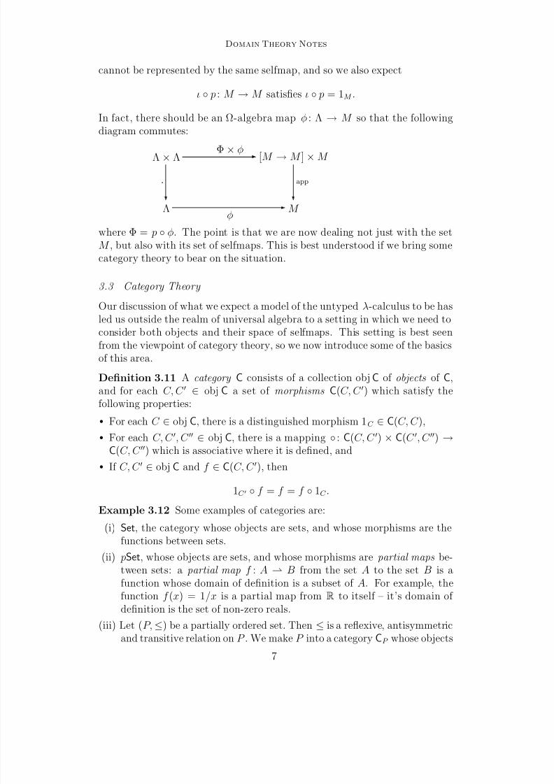
In fact, there should be an Ω-algebra map φ : Λ → M so that the followingdiagram commutes:

Λ × Λ [M → M ] × M

Λ M

Φ × φ

app·

φ

where Φ = p φ. The point is that we are now dealing not just with the setM , but also with its set of selfmaps. This is best understood if we bring somecategory theory to bear on the situation.

3.3 Category Theory

Our discussion of what we expect a model of the untyped λ-calculus to be hasled us outside the realm of universal algebra to a setting in which we need toconsider both objects and their space of selfmaps. This setting is best seenfrom the viewpoint of category theory, so we now introduce some of the basicsof this area.

Definition 3.11 A category C consists of a collection objC of objects of C,and for each C, C ∈ obj C a set of morphisms C(C, C ) which satisfy thefollowing properties:

• For each C ∈ obj C, there is a distinguished morphism 1C ∈ C(C, C ),

• For each C, C , C ∈ obj C, there is a mapping : C(C, C ) × C(C , C ) →C(C, C ) which is associative where it is defined, and

• If C, C ∈ obj C and f ∈ C(C, C ), then

1C f = f = f 1C .

Example 3.12 Some examples of categories are:

(i) Set, the category whose objects are sets, and whose morphisms are thefunctions between sets.

(ii) pSet, whose objects are sets, and whose morphisms are partial maps be-tween sets: a partial map f : A B from the set A to the set B is afunction whose domain of definition is a subset of A. For example, thefunction f (x) = 1/x is a partial map from R to itself – it’s domain of definition is the set of non-zero reals.

(iii) Let (P, ≤) be a partially ordered set. Then ≤ is a reflexive, antisymmetricand transitive relation on P . We make P into a category CP whose objects

7



Domain Theory Notes

are the elements of P , and for each x, y ∈ P , we define

CP (x, y) =

x → y, if x ≤ y, and

∅, otherwise.

(iv) Pos, the category of partially ordered sets, and monotone maps – i.e., themorphisms are those mappings f : P → Q between partially ordered setsP and Q that preserve the order: if x ≤P y, then f (x) ≤Q f (y).

Exercise 3.13 Show that each of the examples above satisfies the conditionsfor being a category. In particular, show that each pair of objects in thecategory has a set of morphisms between them, verify that is associativewhere defined, and identify the identity map 1C for each object C ,

Definition 3.14 A diagram in a category C is a function ∆: D → C whereD = (V, E ) is a directed graph, and ∆ maps vertices v ∈ V to objects ∆(v) ∈obj C, and edges e = v → w ∈ E to morphisms ∆(e) ∈ C(∆(v, ∆(w)).

The diagram ∆: D → C is said to commute if, for all u,v,w ∈ V if e =u → v ∈ E, e = v → w ∈ E and e = u → w ∈ E , then ∆(e) ∆(e) = ∆(e).

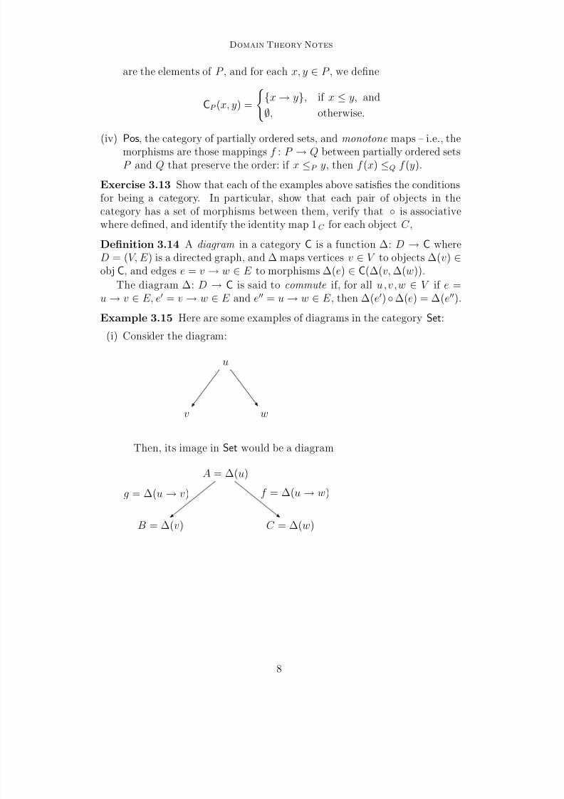
Example 3.15 Here are some examples of diagrams in the category Set:

(i) Consider the diagram:

u

v w

Then, its image in Set would be a diagram

A = ∆(u)

B = ∆(v) C = ∆(w)

f = ∆(u → w)g = ∆(u → v)

8



Domain Theory Notes

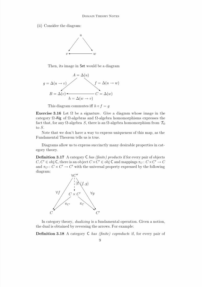
(ii) Consider the diagram:

u

v w

Then, its image in Set would be a diagram

A = ∆(u)

B = ∆(v) C = ∆(w)

h = ∆(w → v)

f = ∆(u → w)g = ∆(u → v)

This diagram commutes iff h f = g

Exercise 3.16 Let Ω be a signature. Give a diagram whose image in thecategory Ω-Alg of Ω-algebras and Ω-algebra homomorphisms expresses thefact that, for any Ω-algebra S , there is an Ω-algebra homomorphism from T Ωto S .

Note that we don’t have a way to express uniqueness of this map, as theFundamental Theorem tells us is true.

Diagrams allow us to express succinctly many desirable properties in cat-

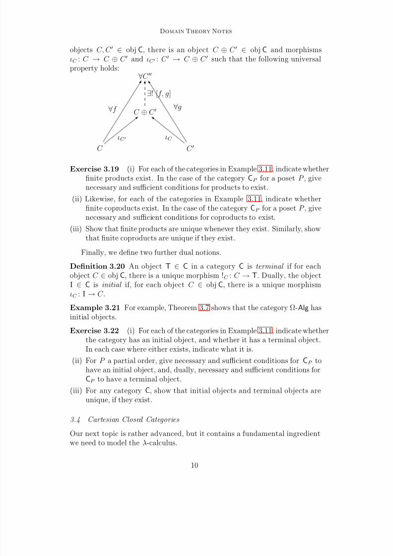
egory theory.Definition 3.17 A category C has (finite) products if for every pair of objectsC, C ∈ obj C, there is an object C ×C ∈ obj C and mappings πC : C ×C → C and πC : C × C → C with the universal property expressed by the followingdiagram:

∀C

C × C

C C

∀f ∀g

∃! f, g

πC πC

In category theory, dualizing is a fundamental operation. Given a notion,the dual is obtained by reversing the arrows. For example:

Definition 3.18 A category C has (finite) coproducts if, for every pair of

9



Domain Theory Notes

objects C, C ∈ obj C, there is an object C ⊕ C ∈ obj C and morphismsιC : C → C ⊕ C and ιC : C → C ⊕ C such that the following universalproperty holds:

∀C

C ⊕ C

C C

∀f ∀g∃! [f, g]

ιC ιC

Exercise 3.19 (i) For each of the categories in Example 3.11, indicate whetherfinite products exist. In the case of the category CP for a poset P , givenecessary and sufficient conditions for products to exist.

(ii) Likewise, for each of the categories in Example 3.11, indicate whetherfinite coproducts exist. In the case of the category CP for a poset P , givenecessary and sufficient conditions for coproducts to exist.

(iii) Show that finite products are unique whenever they exist. Similarly, showthat finite coproducts are unique if they exist.

Finally, we define two further dual notions.

Definition 3.20 An object T ∈ C in a category C is terminal if for eachobject C ∈ obj C, there is a unique morphism !C : C → T. Dually, the objectI ∈ C is initial if, for each object C ∈ obj C, there is a unique morphism

ιC : I → C .

Example 3.21 For example, Theorem 3.7 shows that the category Ω-Alg hasinitial objects.

Exercise 3.22 (i) For each of the categories in Example 3.11, indicate whetherthe category has an initial object, and whether it has a terminal object.In each case where either exists, indicate what it is.

(ii) For P a partial order, give necessary and sufficient conditions for CP tohave an initial object, and, dually, necessary and sufficient conditions forCP to have a terminal object.

(iii) For any category C, show that initial objects and terminal objects areunique, if they exist.

3.4 Cartesian Closed Categories

Our next topic is rather advanced, but it contains a fundamental ingredientwe need to model the λ-calculus.

10



Domain Theory Notes

Definition 3.23 The category C is cartesian closed if

• C has finite products,

• C has a terminal object, and

• (∀A, B ∈ obj C)(∃BA ∈ obj C)(∃ app ∈ C(BA × A, A)) satisfying:

(∀C ∈ obj C)(∀g ∈ C(C × B → A))(∃! curry(g) : C → BA

)so that the following commutes:

BA × A B

C × A C

BA

∀gcurry(g) × 1A

app

∃! curry(g)

Example 3.24 • Set is cartesian closed.

• Pos is cartesian closed.

• If P is a poset, then CP is a ccc iff P has finite meets, a largest element,and, for each x, y ∈ P , x ⇒ y ≡ ∨z ∈ P | x ∧ z ≤ y exists.

• Let V denote the category of finite dimensional vector spaces over R andlinear maps between them. Show that V is cartesian closed:· V has finite products,· the 0-dimensional space 0 is a terminal object for V, and

· The internal hom is just the family of linear maps between the spaces –i.e., W V = V(W, V ) ∈ V..

Also characterize the constant maps in V(W, V ) for any vector spaces W and V .

Exercise 3.25 Show that each of the examples listed is a ccc.

We now list a number of results will be useful in what follows.

Exercise 3.26 Let C be a cartesian closed category, and let A,B,C ∈ obj C.Then,

(i) If f, g ∈ C →C

(A, B) and app (f × 1A) = app (g × 1A), then f = g.(ii) Taking C = B in (i), and considering πB : B × A → B, we get a unique

mapping κAB : B → BA satisfying app (κA

B × 1A) = πB. This is the so-called constant picker which associates to each x ∈ B the constant mapa → x : A → B.

(iii) We next consider

app (1C B × app): C B × (BA × A) → C

11



Domain Theory Notes

and apply the universal property to define a unique map

CBA : C B × BA → C A.

Show this is well-defined, and that, for any D ∈ obj C, we have

D(CBA) : DC × (C B × BA) → DA

and(DCB)A : (DC × C B) × BA → DA

are the same.

Reflexive Objects

We now define those objects in a cartesian closed category that can serveas models for the untyped λ-calculus.

Definition 3.27 If C is a ccc, and object C ∈ obj C is reflexive if

(∃ι : C C → C )(∃r : C → C C ) r ι = 1C C .

Note that this implies that ι is monic.

For example, any singleton set x is reflexive in Set and in Pos (whenendowed with the discrete order). However,

Proposition 3.28 (i) If A is a set with more than one element, then A isnot reflexive in Set.

(ii) Likewise, if P is a poset with more than one element, then P is not reflexive in Pos.

Proof. For (i), we first note that a set A with |A| ≥ 2 has the propertythat there is an injection φ : 2 = 0, 1 → A. Then, we define a mappingΦ : 2A → AA by Φ(f ) = φ f . We claim that Φ is injective. Indeed, if f = g : A → 2 are given, then for some a ∈ A, f (a) = g(a). Since φ isinjective, φ(f (a)) = φ(g(a)), so Φ(f ) = φ f = φ g = Φ(g).

Now, since there is an injection of 2A into AA, it follows that |AA| ≥ |2A| >|A|. So, there cannot be an injection of AA into A, and this means A cannotbe reflexive in Set.

A similar argument can be made for Pos, relying on the fact, due to Gleasonand Dilworth, that any poset with more than one element has the property

that there is no injection of its set of lower sets into itself (this is the analogof Cantor’s Lemma for sets in the category Pos). 2

4 Properties of a Model

We now compile some results about models of the untyped λ-calculus in acartesian closed category. The main result will be to show that reflexive

12



Domain Theory Notes

objects, under suitable assumptions, can serve as models.

4.1 Combinatory Results

We need some results about combinators in the λ-calculus. Recall the syntax

of the untyped λ-calculus is given by

t ::= c | x | tt | λx.t,

where c ∈ C is a prescribed family of constants, and x ∈ V ranges over a setof variables. Recall also the following reduction rules:

(α) λx.m ≡ λy.m[y/x] if y is not free in m.

(β ) (λx.m)n ≡ m[n/x]

(η) λx.mx ≡ m if x is not free in m.

The following are standard combinators of the λ-calculus:

K ≡ λxy.x

S ≡ λxyz.xz(yz)

Y ≡ λf.(λv.f (vv))(λv.f (vv))

I ≡ λx.x

Proposition 4.1 Assuming (β ):

(i) (SK )K ≡ I , so S and K generate.

(ii) For any term f , f (Y f ) ≡ Y F . This means every term has a fixed point in a model of the untyped λ-calculus that validates (β ).

Proof. This is an exercise. 2

The untyped λ-calculus also admits an internal definition of composition,as a derived operator.

Definition 4.2 Define : Λ × Λ → Λ by (m, n) = λx.m(nx), where x is notfree in m or n. We also write m n for (m, n).

Exercise 4.3 Show that, assuming (β ), then (m n) p = m(np).

Exercise 4.4 An ultra-metric on a set X is a function d : X × X → X satis-

fying, for all x,y,z ∈ X :• d(x, y) = 0 iff x = y,

• d(x, y) = d(y, x), and

• d(x, z) = maxd(x, y), d(y, z)

Recall that a Cauchy sequence in a metric space is a sequence xnn∈N suchthat, for each > 0, there is some N ∈ N with d(xm, xn) < (∀m, n ≥ N ).Further, a metric space is complete if each Cauchy sequence has a limit point.

13



Domain Theory Notes

Finally, a mapping f : X → Y between metric spaces is non-expansive if dY (f (x), f (x)) ≤ d(x, x) for all x, x ∈ X .

Show that the category UMet of complete ultra-metric spaces and non-expansive maps is cartesian closed, where we define

d(f, g) = sup|d(f (x), g(x))| | x ∈ X .

Furthermore, show that for any non-degenerate X ∈ obj UMet, there is a non-expansive selfmap f : X → X without a fixed point. This observation is dueto Plotkin.(Hint: show that, for any > 0, B(x) = y | d(x, y) ≤ is open and closed, for every x ∈ X . Conclude that the paradoxical combinator Y ≡λf.(λv,f (vv))(λv.f (vv)) has no interpretation in UMet.)

4.2 Semantic Environments

If we are given a term m with free variables, then we need to have valuesto assign to them if we want to evaluate the term. This role is played byenvironments in a model.

We begin with the assumption that we have a reflexive object C ∈ C ina cartesian closed category with (at least) finite products. We also assumethat we are given an interpretation c → [|c|] ∈ C of each constant c in oursyntax. We let C V denote V -many copies of C ; we note that if C has onlyfinite products (it at least has these since it is a ccc), then this only makessense if V is finite. We won’t see any problem here – it lies in the fact thatsubstitution is problematic in this case.

Definition 4.5 A semantic environment is an assignment σ : V → C , assign-ing to each variable an element of C . Thus, C V denotes the set of semanticenvironments.

Definition 4.6 Let x ∈ C , v ∈ V , and let σ ∈ C V . Then we define a newenvironment σx/v by

σx/v(w) =

σ(w), if w = v,

x, if w = v.

Thus, σx/v replaces σ’s value at v with x.

Lemma 4.7 Let x, y ∈ C , u, v ∈ V and let σ ∈ C V . Then

σx/uy/v =

σy/vx/u, if u = v,

σy/v, if u = v.

Proof. Exercise. 2

14



Domain Theory Notes

This shows that changing the values of an environment in some of itsvariables acts as expected. The question is whether this can be done us-ing morphisms in the category C . Certainly, for those variables w = v,σx/v(w) = σ(w) = πw(σ) is a morphism of C , since C has finite prod-ucts. The other component – v – requires more work.

Proposition 4.8 If C ∈ obj C is a reflexive object in a cartesian closed cat-egory and x ∈ C , then κx : C → C by κx(y) = x satisfies κx ∈ C C .

Proof. This is just Exercise 3.26. 2

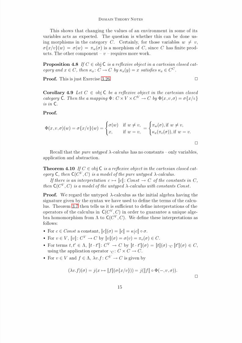
Corollary 4.9 Let C ∈ obj C be a reflexive object in the cartesian closed category C. Then the a mapping Φ : C × V × C V → C by Φ(x,v,σ) = σx/vis in C.

Proof.

Φ(x,v,σ)(w) = σx/v(w) =

σ(w) if w = v,

x, if w = v,=

πw(σ), if w = v,

κx(πv(σ)), if w = v.

2

Recall that the pure untyped λ-calculus has no constants – only variables,application and abstraction.

Theorem 4.10 If C ∈ obj C is a reflexive object in the cartesian closed cat-egory C, then C(C V , C ) is a model of the pure untyped λ-calculus.

If there is an interpretation c → [|c|] : Const → C of the constants in C ,then C(C V , C ) is a model of the untyped λ-calculus with constants Const.

Proof. We regard the untyped λ-calculus as the initial algebra having thesignature given by the syntax we have used to define the terms of the calcu-lus. Theorem 3.7 then tells us it is sufficient to define interpretations of theoperators of the calculus in C(C V , C ) in order to guarantee a unique alge-bra homomorphism from Λ to C(C V , C ). We define these interpretations asfollows:

• For c ∈ Const a constant, [|c|](σ) = [|c|] = κ[|c|] σ.

•

For v ∈ V , [|v|] : C

V

→ C by [|v|](σ) = σ(v) = πv(σ) ∈ C .• For terms t, t ∈ Λ, [|t · t|] : C V → C by [|t · t|](σ) = [|t|](σ) ·C [|t|](σ) ∈ C ,

using the application operator ·C : C × C → C .

• For v ∈ V and f ∈ Λ, λv.f : C V → C is given by

(λv.f )(σ) = j(x → [|f |](σx/v)) = j([|f |] Φ(−, v , σ)).

2

15



Domain Theory Notes

4.3 Functors and Natural Transformations

We now continue our discussion of category theory.

Definition 4.11 Let C and D be categories. A functor F : C → D is a fam-ily of mappings F : objC → obj D and, for each C, C ∈ obj C, a mapping

F : C(C, C ) → D(F (C ), F (C )) satisfying• F (1C ) = 1F (C ) for each C ∈ obj C, and

• If f ∈ C(C, C ) and g ∈ C(C , C ), then F (g f ) = F (g) F (f ).

Example 4.12 (i) Let Grp denote the category of groups and group homo-morphisms. Then there is a functor | | : Grp → Set which forgets thegroup structure on each group and simply remembers that a group is aset, and that a homomorphism between groups is a function between theunderlying sets.

(ii) P : Set → Posop by P (X ) is the power set of X , and for f : X → Y ,

P (f ) : P (Y ) → P (X ) is P (f )(A) = f −1

(A). This is an example of acontravariant functor: it reverses the direction of the morphisms. Hencethe need to label Pos with the superscript op.

Exercise 4.13 Recall Exercise 3.26. The setting is a cartesian closed categoryC. We extend it with the following observations:

(i) If C ∈ obj C, then there is an endofunctor CC : C → C given by CC (A) =AC for A ∈ obj C, and CC : C(A, B) → C(AC , BC ) by CC (f ) = f −.

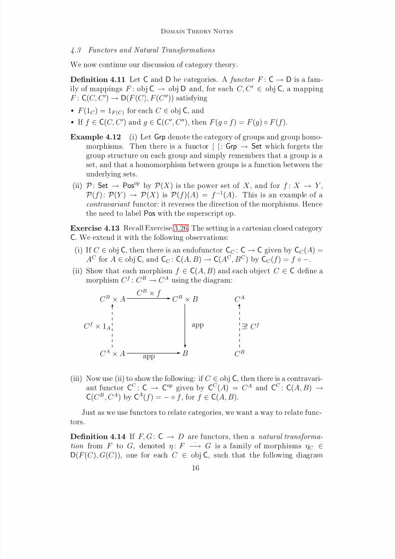
(ii) Show that each morphism f ∈ C(A, B) and each object C ∈ C define amorphism C f : C B → C A using the diagram:

C B × A C B × B

C A × A B C B

C A

app

app

C f × 1A

C B

× f

∃! C f

(iii) Now use (ii) to show the following: if C ∈ obj C, then there is a contravari-

ant functorCC

:C

→Cop

given byCC

(A) = C

A

andCC

:C

(A, B) →C(C B, C A) by CA(f ) = − f , for f ∈ C(A, B).

Just as we use functors to relate categories, we want a way to relate func-tors.

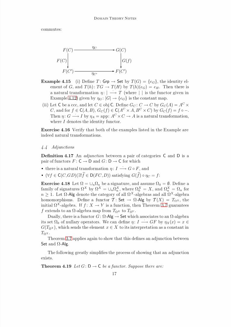
Definition 4.14 If F, G : C → D are functors, then a natural transforma-tion from F to G, denoted η : F

·−→ G is a family of morphisms ηC ∈

D(F (C ), G(C )), one for each C ∈ obj C, such that the following diagram

16



Domain Theory Notes

commutes:

F (C ) G(C )

F (C ) F (C )

ηC

G(f )F (C )

ηC

Example 4.15 (i) Define T : Grp → Set by T (G) = eG, the identity el-ement of G, and T (h) : T G → T (H ) by T (h)(eG) = eH . Then there is

a natural transformation η : |·

−→ T (where | | is the functor given inExample 4.12) given by ηG : |G| → eG is the constant map.

(ii) Let C be a ccc, and let C ∈ obj C. Define GC : C → C by GC (A) = AC ×C , and for f ∈ C(A, B), GC (f ) ∈ C(AC × A, BC × C ) by GC (f ) = f −.

Then η : G ·−→ I by ηA = app: AC × C → A is a natural transformation,where I denotes the identity functor.

Exercise 4.16 Verify that both of the examples listed in the Example areindeed natural transformations.

4.4 Adjunctions

Definition 4.17 An adjunction between a pair of categories C and D is apair of functors F : C → D and G : D → C for which

• there is a natural transformation η : I ·

−→ G F , and

• (∀f ∈ C(C,GD)(∃! f ∈ D(FC,D)) satisfying G( f ) ηC = f :

Exercise 4.18 Let Ω = ∪nΩn be a signature, and assume Ω0 = ∅. Define afamily of signatures ΩX by ΩX = ∪nΩX

n , where ΩX0 = X , and ΩX

n = Ωn forn ≥ 1. Let Ω-Alg denote the category of all ΩX-algebras and all ΩX-algebrahomomorphisms. Define a functor T : Set → Ω-Alg by T (X ) = T ΩX , theinitial ΩX-algebra. If f : X → Y is a function, then Theorem 3.7 guaranteesf extends to an Ω-algebra map from T ΩX to T ΩY .

Dually, there is a functor G : Ω-Alg → Set which associates to an Ω-algebraits set Ω0 of nullary operators. We can define η : I

·−→ GF by ηX(x) = x ∈

G(T ΩX

), which sends the element x ∈ X to its interpretation as a constant inT ΩX .

Theorem 3.7 applies again to show that this defines an adjunction betweenSet and Ω-Alg.

The following greatly simplifies the process of showing that an adjunctionexists.

Theorem 4.19 Let G : D → C be a functor. Suppose there are:

17



Domain Theory Notes

• A mapping of objects F : objC → obj D,

• For each C ∈ obj C, a morphism ηC : C → GF (C )), and

• For each D ∈ obj D and each f ∈ C(C,GD), a unique morphism f ∈

D(FC,D) satisfying f =

f ηC .

Then F : C → D extends uniquely to a functor satisfying (F, G) is an adjunc-tion with natural transformation η : I

·−→ GF .

Example 4.20 The Theorem eliminates some of the work from the previousexercise: it allows us to conclude that T Ω : Set → Ω-Alg is a functor just onthe basis of Theorem 3.7.

4.5 Cones, Limit Cones and Colimit Cocones

Definition 4.21 Let ∆: D → C be a diagram in a category C. A conefor ∆ consists of an object C ∈ obj C and, for each x ∈ D, a morphismf x ∈ C(C, ∆(x)) satisfying ∆(x → y) f x = f y for x, y] ∈ D with x → y ∈ D.

The family (C, f xx∈D is a limit cone for D if, for any cone (C , gxx∈D),there is a unique mediating morphism f ∈ C(C , C ) satisfying gx = f x f foreach x ∈ D.

The notions of cocone and colimit cocone are defined dually.

Example 4.22 Products are examples of limit cones, and coproducts areexamples of colimit cocones in any category where they exist.

Definition 4.23 The category is complete if all cones have limit cones, andit is cocomplete if all cocones have colimit cocones.

5 ω-Complete Partial Orders

We now introduce a category in which we actually can construct a model of the untyped λ-calculus. We choose perhaps the simplest such category – thereare several others whose definitions require more intricate concepts.

Definition 5.1 A partially ordered set P is ω-complete if every increasingchain xnn∈N ⊆ P has a least upper bound in P .

Example 5.2

• For any set X , the power set (P (X ), ⊆) is ω-complete. More generally, any

complete lattice is ω-complete.• ([0, 1], ≤) – the unit interval in the usual order is ω-complete.

• Likewise, ([0, 1) ∪ 2, ≤) is ω-complete, where now n(1 − 1/n) = 2.

• On the other hand, (R, ≤) is not ω-complete; nor is (Q ∩ [0, 1], ≤), therationals in the unit interval.

Definition 5.3 A function f : P → Q is continuous if f is monotone and f preserves suprema of increasing chains.

18



Domain Theory Notes

We let Ω−Pos denote the category of ω-complete partial orders and con-tinuous maps.

Here are some examples of continuous maps between ω-continuous partialorders.

Example 5.4• f : ([0, 1], ≤) → ([0, 1) ∪ 2, ≤) by

f (x) =

x if x < 1,

2, if x = 1.

• For any set X , f : (P (X ), ⊆) → (P (X ), ⊇) by f (A) = X \ A.

• If P is an ωcomplete partial order, then so is (P, =), P endowed with thediscrete order . Then the identity map 1P : (P, =) → (P, ≤) is continuous.

Theorem 5.5 Ω−Pos has all products and coproducts.

Proof. We show the result for products, and for finite coproducts.

For products, let P ii∈I be family of ω-complete partial orders. We takei P i to be the usual product (i.e., the one from Set), and we endow this with

the partial order: xii∈I ≤ yii∈I iff xi ≤ yi for every i ∈ I . Clearly, this isthe same as saying x ≤ y ∈

i P i iff πi(x) ≤ πi(y for every i ∈ I , so that the

projection maps are not only monotone, they in fact define the order.

If xnn∈N is an increasing chain in

i P i, then m ≤ n ∈ N impliesπi(xm) ≤ πi(xn), so πi(xm)m∈N is an increasing chain in P i. As such, ithas a least upper bound, xi ∈ P i, and then x ∈ i P i by πi(x) = xi is clearly

an upper bound for xnn∈N. And, if xn ≤ y ∈ i P i for every n ∈ N, thenπi(xn) ≤] pii(y) for every n, for each i ∈ I . Then xi = nπi(xn) ≤ πi(y),so x ≤ y. Thus xnn∈N has a least upper bound in

i P I , and we also can

conclude that each projection πi :

i P I → P i is continuous.

Now, if Q ∈ Ω−Pos and if f i : Q → P i is continuous for each i ∈ I ,then we define f ii∈I : Q →

i P i by f ii∈I (q) = f i(q)i∈I . By definition,

πi f ii∈I = f i, and since f i is continuous and the πis define the order oni P i, we conclude that f ii∈I is continuous. The mapping clearly is the

unique f : Q →

i P i satisfying πif by definition. This shows

i P i deservesits name.

For coproducts, let P, Q ∈ objΩ−Pos. Define P + Q = 0 × P ∪ 1 × Q,where we assume 0, 1 ∈ P ∪ Q. Then this is a disjoint union. We define(a, b) ≤ (c, d) in P + Q iff a = c and b ≤ d in whichever component they bothreside in – for a = c = 0, they are in P , while if a = c = 1, then they both arein Q. This is clearly a partial order, and any ω-chain in P + Q must either bein P or in Q; in either case, the chain has its least upper bound defined as inP or Q, respectively.

Define mappings ιP : P → P + Q by ιP (x) = (0, x, and likewise, ιQ : Q →

19



Domain Theory Notes

P + Q by ιQ(y) = ( 1, y). It is routine to verify these mappings are ω-continuous.

Finally, given continuous maps f : P → Q and g : Q → R, we define[f, g] : P + Q → R by [f, g](0, x) = f (x), and [f, g](1, y) = g(y). This defines aunique continuous map from P +Q to R whose composition with the coproduct

maps ιP and ]iotaQ yields f and g, respectively. This shows P + Q is thecoproduct of P and Q in Ω−Pos. 2

Exercise 5.6 Generalize the definition of the coproduct given in the previousproof to show that Ω−Pos has all coproducts.

5.1 Function Spaces

We now show that the function space of continuous maps between ω-complete

partial orders is another such.

Definition 5.7 If f, g ∈ Ω−Pos(P, Q), then we define f ≤ g iff f (x) ≤ g(x)for every x ∈ P .

Theorem 5.8 Ω−Pos(P, A) ∈ Ω−Pos for every P, Q ∈ objΩ−Pos.

Proof. Let f n ∈ Ω−Pos(P, Q) for each n ∈ N with f m ≤ f n for m ≤ n. Definef : P → Q by f (x) = f f n(x), for each x ∈ P . This is well-defined, becausef n(x)n∈N is increasing in Q, which is ω-complete. It also is clear that f ismonotone. Let xm] m ∈ N ⊆ P be an increasing chain, and let x = mxm.Then

f (x) = (nf n)(x) = nf n(x) by definition

= nf n(mxm) = n(mf n(xm)) since f n is continuous

= m,nf n(xm) = m(nf n(xm)) since suprema commute

= mf (xm).

2

It’s not only true that Ω−Pos has function spaces, but in fact it’s easy forfunctions defined on a product of ω-complete posets to be continuous.

Proposition 5.9 Let f : P × Q → R be a function from the product of ω-complete posets to another such, The following are equivalent:

(i) f is continuous.

(ii) f is continuous in each variable separately.

Proof. Suppose f is continuous in each variable separately. It is routineto show this implies f is monotone. Now, let (xn, yn)n∈N ⊆ P × Q be anincreasing chain. Then

20



Domain Theory Notes

f (n(xn, yn)) = f ((mxm, nyn))

= mf ((xm, nyn))

= m n f ((xm, yn))

= nf ((xn, yn)),

where the first and last equalities follow from the facts that xm, yn are increas-ing and f is monotone, and the middle two rely on the separate continuity of f 2

5.2 Ω−Pos is Cartesian Closed

We now turn our attention to showing that Ω−Pos is cartesian closed. Wealready have most of the ingredients – Ω−Pos has an internal hom, the functionspace, and it is closed under products, so it also has a terminal object, theone-point space. It only remains to verify the required properties hold.

Theorem 5.10 Ω−Pos

is cartesian closed.Proof. We’ve already remarked that all the ingredients we need are available– products, a terminal object and function spaces. So, support that P,Q,R ∈objΩ−Pos. Then QP ≡ Ω−Pos(P, Q) ∈ objΩ−Pos, and we define app: QP ×P → Q by app(f, x) = f (x). This is clearly well-defined, and it’s easy to seeit is monotone. If f n ∈ QP is increasing and f = nf n, then for any x ∈ P ,

app(f, x) = f (x) = (nf n)(x) = nf n(x),

by definition of nf n. Likewise, if f ∈ QP and xnn∈N ⊆ P is increasing withx = nxn, then

app(f, x)f (nxn) = nf (xn)

since f is continuous. This shows that app is continuous in each variableseparately, and so Proposition 5.9 implies app is jointly continuous.

Now suppose g : R×P → Q, and define curry(g) : RQP by curry(g)(x) : P →Q by curry(g)(x)(y) = g(x, y). Proposition 5.9 implies curry(g)(x) ∈ Ω−Pos(P, Q),and, equally, that this assignment is continuous in x ∈ R. Clearly app curry(g) = g, and certainly this defines curry(g) uniquely. 2

5.3 Tarski’s Theorem

Of course, we also are interested in finding non-degenerate reflexive objects inΩ−Pos, but to do that, we need more category theory. Before pursuing that,however, we first prove a classical result about ω-complete partial orders,which also provides a hint of how we’ll seek to prove there are non-degeneratemodels on the untyped λ-calculus in Ω−Pos.

Theorem 5.11 (Tarksi, Knaster, Scott) Let f ∈ Ω−Pos where P has a least element. Then f has a least fixed point fix(f ) = nf n(⊥).

21



Domain Theory Notes

Proof. Since ⊥ is the least element of P , we have ⊥≤ f (⊥). Since f ismonotone, applying f to this inequality shows that f n(⊥) ≤ f n+1(⊥), byinduction on n. Hence f n(⊥)n∈N is an increasing sequence in P , and soit has a least upper bound, which we denote by fix(f ). Indeed, since f iscontinuous,

f (fix(f )) = f (nf n(⊥) = nf n+1(⊥) = fix(f ).

The fact that fix(f ) is f ’s least fixed point is an easy argument. 2

Exercise 5.12 Show that fix(f ) is indeed the least fixed point of f .

Exercise 5.13 Consider [N N], the space of partially defined selfmaps of N, where we give N the flat order.

(i) Order [N N] by

f ≤ g ⇔ dom(f ) ⊆ dom(g) & g|dom(f ) = f.

Show that [N N] ∈ Ω−Pos.

(ii) Define F : [N N] → [N N] by

F (f )(n) =

1, if n = 0

(n + 1) ∗ f (n), if n > 0.

Show that F is ω-continuous, and fix(F ) = fac: N → N.

6 F -algebras and Continuous Functors

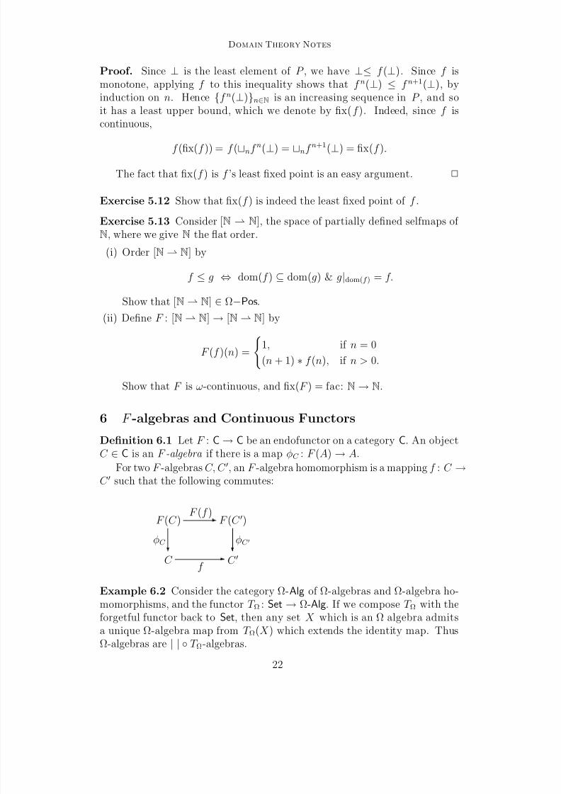
Definition 6.1 Let F : C → C be an endofunctor on a category C. An objectC ∈ C is an F -algebra if there is a map φC : F (A) → A.

For two F -algebras C, C , an F -algebra homomorphism is a mapping f : C →C such that the following commutes:

F (C ) F (C )

C C

F (f )

φC φC

f

Example 6.2 Consider the category Ω-Alg of Ω-algebras and Ω-algebra ho-momorphisms, and the functor T Ω : Set → Ω-Alg. If we compose T Ω with theforgetful functor back to Set, then any set X which is an Ω algebra admitsa unique Ω-algebra map from T Ω(X ) which extends the identity map. ThusΩ-algebras are | | T Ω-algebras.

22



Domain Theory Notes

Theorem 6.3 For an endofunctor F : C → C, if C ∈ obj C is an initial F -algebra, then the mapping φC : F (C ) → C is an isomorphism.

Proof. Exercise. 2

6.1 Adjunctions Between Posets

Definition 6.4 A pair of mappings f : P → Q and g : Q → P form an adjunction if

(∀x ∈ P )(∀y ∈ Q) x ≤P g(y) ⇔ f (x) ≤Q y.

Example 6.5

(i) Suppose P has a least element, ⊥, and define κ : P → Pos(P, P ) byκ(x)(y) = x, and !: Pos(P, P ) → P by !(f ) = f (⊥). Then

x ≤P !f ⇔ x ≤P f (⊥) ⇔ x ≤ f (y) (∀y) ⇔ κ(x) ≤ f.

(ii) Let A be a poset with a least element, and for a poset P , let Q = A × P in the product order. Define f : Q → P to be the projection map, andlet g : P → Q by g(x) = (⊥A, x). Then (f, g) is an adjunction:

(a, x) ≤ g(x) ⇔ x = f (a, x) ≤ x.

(iii) Let P have a least element, ⊥, and define κ : P → Pos(P, P ) by κ(x)(y) =x, and !: Pos(P, P ) → P by !(f ) = f (⊥). Then

x ≤P !f ⇔ x ≤P f (⊥) ⇔ x ≤ f (y) (∀y) ⇔ κ(x) ≤ f.

Theorem 6.6 Given a pair of monotone maps f : P → Q and g : Q → P ,the following are equivalent:

(i) The pair (f, g) is an adjunction.

(ii) f g ≤ 1Q and g f ≥ 1P .

(iii) (∀x ∈ P ) f (x) = inf g−1(↑ x), and ∀y ∈ Q) g(y) = sup f −1(↓ y).

In this case, f preserves all existing suprema, and g preserves all existing infima. Finally, each of these conditions implies

• f = f g f and g = g f g.

Proof. Exercise. 2

Definition 6.7 The upper adjoint f is called an embedding if g f = 1P . Inthis case, g is called a projection .

Corollary 6.8 The functors listed above cut down to a dual equivalence be-tween the categories Ω−Pose and Ω−Pos p whose morphisms are embedding,respectively, projections.

Exercise 6.9 Show that embeddings are one-to-one, and that projections areonto.

23



Domain Theory Notes

Remark 6.10 Let f : P → Q and g : Q → P be an adjunction. Then,

(i) f is called the lower adjoint and g is called the upper adjoint .

(ii) This result does not require that f or g be continuous – in fact, it showsthat f must be continuous.

Exercise 6.11 Show that the conditions above are equivalent to f : P → Qand g : Q → P being adjoint functors, if P and Q are viewed as categories.

We define:Ω−PosU – ω-complete posets and upper adjoints.Ω−PosL – ω-complete posets and lower adjoints.

Theorem 6.12 There are adjoint functors

U : Ω−PosL → Ω−Pos

opU and

L : Ω−Pos

opU → Ω−PosL

which form a dual equivalence, where:

• P L = P and f L = g, the lower adjoint of f , and

• P U = P and gU = f , the upper adjoint of g.

Proof. Straightforward. 2

6.2 Projective Limits

Definition 6.13 A an ordered set D is directed if every finite subset F ⊆ Dhas a least upper bound in D. A projective diagram in a category C is adiagram ∆: D → C in which D is a directed set.

Proposition 6.14 The category Ω−Pos p has projective limits.

Proof. Recall

i∈D ∆(i) is in Ω−Pos. Given the diagram ∆: D → Ω−Pos p,consider the set

P = (xi)i∈D ∈i

∆(i) | i ≤ j ∈ D ⇒ f ij(x j) = xi.

This is closed in

i ∆(i) because the bonding maps - f ij - are continuous.Define πi|P : P → ∆(i) – this is an upper adjoint to

ei : ∆(i) → P by (ei(x)) j = f jk gik(x) where i, j ≤ k ∈ D.

Suppose Q ∈ objΩ−Pos and hi ∈ Ω−Pos(Q, P i) with f ij h j = hi for eachi ≤ j ∈ D. Defining

h ∈ Ω−Pos(Q, P ) by (h(x))i = hi(x),

yields a unique continuous map with gij(h(x) j) = h(x)i. 2

24



Domain Theory Notes

Exercise 6.15

(i) Show that πi : P → P i is surjective for each i ∈ D. Conclude that P = ∅.

(ii) Show that the mapping ei : ∆(i) → P is well-defined – i.e., show that,given any j ∈ D, for any choices k, k ∈ D with i, j ≤ k, k, we havef jk gik = f jk gik .

(iii) Show that the mediating map h : Q → P does satisfy the conditionsneeded.

6.3 Inductive Limits

Theorem 6.16 If (P i, gij)i≤ j∈D is a projective system in Ω−Pos p, and (P i, f ij)i≤ j∈Dis the associated system of lower adjoints in Ω−Pose, then

lim(P i, gij)i≤ j∈D colim(P i, f ij)i≤ j∈D.

Proof. We know lim(P i, gij)i≤ j∈D exists, and since U

and L form a dualequivalence, the latter takes existing limits to colimits in the dual category.But U and L are both the identity on objects, so if P = lim(P i, gij)i≤ j∈D,then

P = P L = (colimP i, f ij)i≤ j∈D.

2

Remark 6.17 It is important to notice here that the limit and colimit havethe same underlying set. This is an example of the so-called “limit-colimitcoincidence:” The fact that limits with projections not only correspond tocolimits with the associated embeddings – they are in fact the same sets.

6.4 Enriched Categories

Definition 6.18 A category C is enriched over Pos if C(P, Q) ∈ Pos for eachP, Q ∈ obj C, and : C(C, C ) × C(C , C ) → C(C, C ) preserves the order.

Let F : C → D be a functor between categories enriched over Pos. Then F is locally monotone if F : C(P, Q) → D(F (P ), F (Q)) preserves the order.

Example 6.19 Let L : Ω−Pos → Ω−Pos! be defined by L(P ) = P ∪ ⊥P ,and L(f ) : L(P ) → L(Q) is

L(f )(x) = f (x), if x ∈ P,⊥Q, if x =⊥P .

Then L is locally monotone: f ≤ g ⇒ L(f ) ≤ L(g).

Lemma 6.20 Let F : C → D be locally monotone, where C and D are subcat-egories of Ω−Pos. If f ∈ C(P, Q) is the upper adjoint of g : Q → P in C, then F (f ) : F (P ) → F (Q) is upper adjoint to F (g) : F (Q) → F (P ) in D.

25



Domain Theory Notes

Proof. Suppose that f : P → Q is a lower adjoint to g : Q → P . Thenf g ≤ 1Q and g f ≥ 1P . Then, applying the locally monotone functor F ,we have

F (f ) F (g) = F (f g) ≤ F (1P ) = 1F (P ),

and

F (g) F (f ) = F (g f ) ≥ F (1Q) = 1F (Q).

2

6.5 Calculating Limits

Definition 6.21 Let A be a subcategory of Ω−Pos. We say A is pro-completeif A is closed in Ω−Pos under the formation of projective limits. Likewise, A isind-complete if A is closed in Ω−Pos under the formation of inductive limits.

Exercise 6.22

(i) Let A be a pro-complete subcategory of Ω−Pos. Then A p, the subcategoryof objects of A with projections in A as morphisms, also is pro-complete.

(ii) Likewise, if A is ind-complete, the so is the subcategory Ae, whose objectsare the same as those of A, and whose morphisms are embeddings.

Theorem 6.23 Let A and B be pro-complete subcategories of Ω−Pos, and let F : A → B be a locally monotone functor which is a left adjoint. Then therestriction F p : A p → B p is pro-continuous.

Proof. The previous lemma shows F has a restriction F p. If (P i, gij)i≤ j∈D isa projective system in A p, then the associated inductive system (P i, f ij)i≤ j∈Dlies in Ae. Moreover, if

(P, gi)i∈D = lim(P i, gij)i≤ j∈D,

then a previous theorem implies

(P, f i)i∈D = colim(P i, f ij)i≤ j∈D.

Since F : A → B is a left adjoint, we have

F p(lim(P i, gij)) = F (lim(P i, gij)) A pro − complete

F (colim(P i, f ij)) previous Theorem colim(F (P i), F (f ij)) left adjoints

preserve colimits

lim(F (P ), F (gij)) F locally monotone and

a previous Theorem

lim(F p(P i), F p(gij)) B pro − complete.

2

26



Domain Theory Notes

Exercise 6.24 Show that if F : C → D and G : D → C form an adjunctionbetween categories, then the left adjoint F preserves all existing colimits, andthe right adjoint G preserves all existing limits.

6.6 Main Result

Corollary 6.25 Let A be a pro-complete subcategory of Ω−Pos containing an initial object ⊥. If F : A → A is a locally monotone, left adjoint and if ! : ⊥→ F (⊥) is an embedding, then there is an initial F -algebra in A, which is necessarily a fixed point for F .

Proof. Since !: ⊥→ F (⊥) is an embedding, there is an upper adjoint ! : F (⊥) →⊥, and so we have a projective sequence (F n(⊥), F m(!) · · · F n−1(!))m≤n∈N. The previous results imply this sequence has a limit, and thatF preserves it:

F (lim(F n−1(⊥), F m(!) · · · F n−1(!))m≤n∈N

lim(F n(⊥), F m+1(!) · · · F n(!))m≤n∈N

(F n(⊥), F m(!) · · · F n−1(!))m≤n∈N

which proves our result. 2

Exercise 6.26 Recall Ω−Pos!, the category of Ω−Pos objects having leastelements, and continuous maps preserving the least element. We definedL : Ω−Pos → Ω−Pos! by L(P ) = P ∪ ⊥P , where L(f ) : L(P ) → L(Q)is

L(f )(x) =

f (x), if x ∈ P,

⊥Q, if x =⊥P .

Then

• L is locally monotone: f ≤ g ⇒ L(f ) ≤ L(g) and : Ω−Pos(P, Q) ×Ω−Pos(Q.R) → Ω−Pos(P, Q) is as well.

• Ω−Pos has an initial object ⊥ for which !: ⊥ → P is an embeddingwith upper adjoint x →⊥ : P → ⊥.

Hence, an initial L-algebra is

lim(Ln(⊥), Lm(

!) · · · Ln−1(

!))m≤n∈N N.

6.7 The Problem for Ω−Pos(P, P )

We would like to apply our main result to a functor which, on objects is givenby P → Ω−Pos(P, P ). However, there’s no clear way to extend this a functor(check this!). Still the following shows us how to proceed:

We define the categoryΩ−Posep – ω-complete posets and embedding-projection pairs.

The following diagram contains the crucial information:

27



Domain Theory Notes

Ω−Pos(P, P ) Ω−Pos(P, P )

Ω−Pos(Q, Q) Ω−Pos(Q)

P

Q

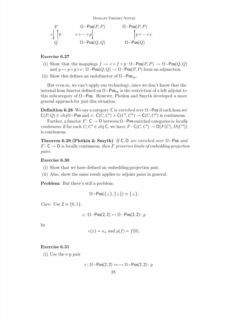
p − ee − pe p

Exercise 6.27(i) Show that the mappings f → e f p : Ω−Pos(P, P ) → Ω−Pos(Q, Q)

and g → p g e : Ω−Pos(Q, Q) → Ω−Pos(P, P ) form an adjunction.

(ii) Show this defines an endofunctor of Ω−Posep.

But even so, we can’t apply our technology, since we don’t know that theinternal hom functor defined on Ω−Posep is the restriction of a left adjoint tothis subcategory of Ω−Pos. However, Plotkin and Smyth developed a moregeneral approach for just this situation.

Definition 6.28 We say a category C is enriched over Ω−Pos if each hom set

C(P, Q) ∈ objΩ−Pos and : C(C, C ) × C(C , C ) → C(C, C ) is continuous.Further, a functor F : C → D between Ω−Pos-enriched categories is locally

continuous if for each C, C ∈ obj C, we have F : C(C, C ) → D(F (C ), D(C ))is continuous.

Theorem 6.29 (Plotkin & Smyth) If C,D are enriched over Ω−Pos and F : C → D is locally continuous, then F preserves limits of embedding-projection pairs.

Exercise 6.30

(i) Show that we have defined an embedding-projection pair.

(ii) Also, show the same result applies to adjoint pairs in general.

Problem: But there’s still a problem:

Ω−Pos(⊥, ⊥) ⊥.

Cure: Use 2 ≡ 0, 1:

e : Ω−Pos(2, 2) ↔ Ω−Pos(2, 2) : p

by

e(x) = κx and p(f ) = f (0).

Exercise 6.31

(i) Use the e-p pair

e : Ω−Pos(2, 2) ←←→ Ω−Pos(2, 2) : p

28



Domain Theory Notes

to generate sequence

(F n(2), F m( p) · · · F n−1( p))m≤n∈N

and show this sequence has a limit with

F (lim(F n

(2), F m

( p)···F n−

1( p))m≤n∈N) (F n

(2), F m

( p)···F n−

1( p))m≤n∈N.

This is the so-called D∞ model that Scott first devised for the untypedλ-calculus.

(ii) More generally, if A is a set of constants over which we define the untypedλ-calculus, then define

F : Ω−Posep → Ω−Posep by F (P ) = A + Ω−Pos(P, P ).

Use above technology to find initial solution:

P F (P ) = A + Ω−Pos(P, P ).

7 Collected Exercises

Here are a number of related exercises from the notes collected together. Theoriginal number of the exercise is included for references (this sometimes canbe the number of a result such as a Theorem, Proposition, etc., in case theexercise was to prove the result):

Strings For an alphabet A (i.e., a non-empty set), a string over A is just afinite sequence a1a2 · · · an, where a1, . . . , an ∈ A (note: the ais need not bedistinct). Two strings s = a1 · · · am and t = a1 · · · an can be concatenated,as in s · t = a1 · · · ana1 · · · am.(i) [3.5(iii)] Give a signature Ω for the set of finite strings over the set A

and concatenation as an operation.(ii) [3.9] Use Corollary 3.7 to define a rank function for the set of finite

strings over a set A, and show that this rank function gives exactly thelength n of a string s = a1 · · · an.

(iii) [4.18] Using the technique of outlined in Exercise 4.18, show that thesignature Ω you defined in the first part can be used to define a familyof signatures ΩA by ΩA = ∪nΩA

n , where ΩA0 = A, and ΩA

n = Ωn forn ≥ 1.

(a) Let Ω-Alg denote the category of all ΩA

-algebras and all ΩA

-algebrahomomorphisms. Define a functor T : Set → Ω-Alg by T (A) = T ΩA,the initial ΩA-algebra. If f : A → B is a function, then use Theorem 3.7to show f extends to an Ω-algebra map from T ΩA to T ΩB .

(b) Dually, show there is a functor G : Ω-Alg → Set which associates to an

Ω-algebra its set of Ω0 of nullary operators. We can define η : I ·

−→ GF by ηA(x) = x ∈ G(T ΩA), which sends the element x ∈ A to its inter-pretation as a constant in T ΩA.

29



Domain Theory Notes

(c) Use Theorem 3.7 to show that this defines an adjunction between Set

and Ω-Alg.

3.26 Let C be a cartesian closed category, and let A,B,C ∈ obj C. Then,(i) If f, g ∈ C → C(A, B) and app (f × 1A) = app (g × 1A), then f = g.

(ii) Taking C = B in (i), and considering πB : B × A → B, we get a unique

mapping κAB : B → BA satisfying app (κAB × 1A) = πB. This is theso-called constant picker which associates to each x ∈ B the constantmap a → x : A → B.

(iii) We next consider

app (1C B × app): C B × (BA × A) → C

and apply the universal property to define a unique map

CBA : C B × BA → C A.

Show this is well-defined, and that, for any D ∈ obj C, we have

D(CBA) : DC × (C B × BA) → DA

and(DCB)A : (DC × C B) × BA → DA

are the same.

4.1ff This is an exercise on the combinators of the λ-calculus. Assuming (β ),show:(i) (SK )K ≡ I , so S and K generate.

(ii) For any term f , f (Y f ) ≡ Y F . This means every term has a fixed pointin a model of the untyped λ-calculus that validates (β ).(iii) If : Λ × Λ → Λ is the composition operator defined in Definition 4.2,

then for all m,n,p ∈ Λ, (m n) p = m(np).

4.7ff Let C be a cartesian closed category and let C ∈ obj C be a reflexiveobject in C.(i) Let x, y ∈ C , u, v ∈ V and let σ ∈ C V . Then

σx/uy/v =

σy/vx/u, if u = v,

σy/v, if u = v.

(ii) Use (i) to show that (α)(see 4.1) and (β )(see 4.1) both hold for theinterpretation of the untyped λ-calculus in C (see 4.10).

(iii) ∗ What about (η)(see 4.1)?

4.13 The setting is a cartesian closed category C. We extend it with thefollowing observations:(i) If C ∈ obj C, then there is an endofunctor CC : C → C given by CC (A) =

AC for A ∈ obj C, and CC : C(A, B) → C(AC , BC ) by CC (f ) = f −.

30



Domain Theory Notes

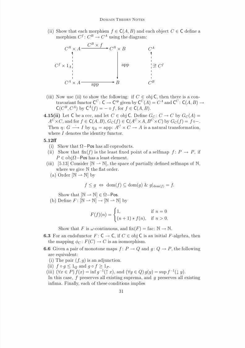
(ii) Show that each morphism f ∈ C(A, B) and each object C ∈ C define amorphism C f : C B → C A using the diagram:

C B × A C B × B

C A × A B C B

C A

app

app

C f × 1A

C B × f

∃! C f

(iii) Now use (ii) to show the following: if C ∈ obj C, then there is a con-travariant functor CC : C → Cop given by CC (A) = C A and CC : C(A, B) →C(C B, C A) by CA(f ) = − f , for f ∈ C(A, B).

4.15(ii) Let C be a ccc, and let C ∈ obj C. Define GC : C → C by GC (A) =

AC

×C , and for f ∈ C(A, B), GC (f ) ∈ C(AC

×A, BC

×C ) by GC (f ) = f −.Then η : G

·−→ I by ηA = app: AC × C → A is a natural transformation,

where I denotes the identity functor.

5.12ff (i) Show that Ω−Pos has all coproducts.

(ii) Show that fix(f ) is the least fixed point of a selfmap f : P → P , if P ∈ objΩ−Pos has a least element.

(iii) [5.13] Consider [N N], the space of partially defined selfmaps of N,where we give N the flat order.

(a) Order [N N] by

f ≤ g ⇔ dom(f ) ⊆ dom(g) & g|dom(f ) = f.

Show that [N N] ∈ Ω−Pos.(b) Define F : [N N] → [N N] by

F (f )(n) =

1, if n = 0

(n + 1) ∗ f (n), if n > 0.

Show that F is ω-continuous, and fix(F ) = fac: N → N.

6.3 For an endofunctor F : C → C, if C ∈ obj C is an initial F -algebra, then

the mapping φC : F (C ) → C is an isomorphism.6.6 Given a pair of monotone maps f : P → Q and g : Q → P , the following

are equivalent:(i) The pair (f, g) is an adjunction.

(ii) f g ≤ 1Q and g f ≥ 1P .(iii) (∀x ∈ P ) f (x) = inf g−1(↑ x), and (∀y ∈ Q) g(y) = sup f −1(↓ y).

In this case, f preserves all existing suprema, and g preserves all existinginfima. Finally, each of these conditions implies

31



Domain Theory Notes

• f = f g f and g = g f g.

6.15 ∗ This is in the context of a projective family (P i, f ij)i≤ j∈D.(i) Show that πi : P → P i is surjective for each i ∈ D. Conclude that

P = ∅.(ii) Show that the mapping ei : ∆(i) → P is well-defined – i.e., show that,

given any j ∈ D, for any choices k, k ∈ D with i, j ≤ k, k, we havef jk gik = f jk gik .

(iii) Show that the mediating map h : Q → P does satisfy the conditionsneeded.

6.26 Recall Ω−Pos!, the category of Ω−Pos objects having least elements,and continuous maps preserving the least element. We defined L : Ω−Pos →Ω−Pos! by L(P ) = P ∪ ⊥P , where L(f ) : L(P ) → L(Q) is

L(f )(x) =

f (x), if x ∈ P,

⊥Q, if x =⊥P .

Then• L is locally monotone: f ≤ g ⇒ L(f ) ≤ L(g) and : Ω−Pos(P, Q) ×

Ω−Pos(Q.R) → Ω−Pos(P, Q) is as well.• Ω−Pos has an initial object ⊥ for which !: ⊥ → P is an embedding

with upper adjoint x →⊥ : P → ⊥.Hence, an initial L-algebra is

lim(Ln(⊥), Lm( !) · · · Ln−1( !))m≤n∈N N.

6.27 This is in the context of defining a functor on Ω−Posep using the internal

hom.(i) Show that the mappings f → e f p : Ω−Pos(P, P ) → Ω−Pos(Q, Q)

and g → p g e : Ω−Pos(Q, Q) → Ω−Pos(P, P ) form an adjunction.(ii) Show this defines an endofunctor of Ω−Posep.

6.28ff (i) Show that Ω−Pos is enriched over Ω−Pos.

(ii) Show that for a given set A of constants over which we define the un-typed λ-calculus, then define

F : Ω−Posep → Ω−Posep by F (P ) = A + Ω−Pos(P, P ).

Use above technology to find initial solution:

P F (P ) = A + Ω−Pos(P, P ).

7.1 Exam Questions

For the examination in the course, work through the following exercises listedabove: Strings, 3.26, 4.7ff, 4.13, 5.12ff, 6.6 and 6.15. Note that ∗

32



Domain Theory Notes

exercises are optional ; this means 4.7(iii) and 6.15 are not required, but arerecommended.

8 Bibliography

Here are some general references for domain theory and related topics. Thisis a minimal list, but it should provide sufficient resources to find the wealthof material available on the subject. For example, there is an especially well-annotated bibliography in [7], and there is a very extensive bibliography in[4].

References

[1] Abramsky, S. and A. Jung, Domain Theory , in: “Handbook of Computer Scienceand Logic,” Volume 3, Clarendon Press, 1995.

[2] Amadio, P. and P.-L. Curien, “Domains and the Lambda Calculus,” CambridgeUniversity Press, 1998.

[3] Asperti, A. and G. Longo, “Categories, Types and Structures,” MIT Press, 1991.

[4] Gierz, G., K. H. Hofmann, K. Keimel, J. Lawson, M. Mislove and D. S. Scott,“Continuous Lattices and Domains,” Cambridge University Press, 2003. This isan updated and expanded version of a classic work by the same authors that nowis out of print:Gierz, G., et al , “A Compendium of Continuous Lattices,” Springer-Verlag, 1980.

[5] Jung, A., “Cartesian Closed Categories of Domains,” CWI Tracts 66, 1989.

[6] Mislove, M. Topology, domain theory and theoretical computer science, Topologyand Its Applications 89 (1998), pp. 3–59.

[7] Pierce, B. J., “Basic Category Theory for Computer Scientists,” MIT Press,1993.

[8] Plotkin, G., “Domains,” Lecture Notes, University of Edinburgh, 1980. Availableon the web athttp://http://www.dcs.ed.ac.uk/home/gdp/publications/Domains.ps.gz .

[9] Stoltenberg-Hansen, V, I. Linstrom and E. R. Griffor, “Mathematical Theory of

Domains,” Cambridge University Press, 1994.

http://http//www.dcs.ed.ac.uk/home/gdp/publications/Domains.ps.gz

http://http//www.dcs.ed.ac.uk/home/gdp/publications/Domains.ps.gz

notes on domain theory by mislove

Documents