NREL is a national laboratory of the U.S. Department of Energy Office of Energy Efficiency & Renewable Energy Operated by the Alliance for Sustainable Energy, LLC This report is available at no cost from the National Renewable Energy Laboratory (NREL) at www.nrel.gov/publications.

Contract No. DE-AC36-08GO28308

Conference Paper NREL/CP-5D00-75273 March 2020

Power-Domain Impedance Theory for the Analysis and Mitigation of Interarea Oscillations PreprintShahil Shah,1 Weihang Yan,1 Vahan Gevorgian,1 and Wenzhong Gao2 1 National Renewable Energy Laboratory2 University of Denver

To be presented at the 2020 IEEE Power and Energy Society General Meeting (IEEE PES GM) Montreal, Canada August 2–6, 2020

NREL is a national laboratory of the U.S. Department of Energy Office of Energy Efficiency & Renewable Energy Operated by the Alliance for Sustainable Energy, LLC This report is available at no cost from the National Renewable Energy Laboratory (NREL) at www.nrel.gov/publications.

Contract No. DE-AC36-08GO28308

National Renewable Energy Laboratory 15013 Denver West Parkway Golden, CO 80401 303-275-3000 • www.nrel.gov

Conference Paper NREL/CP-5D00-75273 March 2020

Power-Domain Impedance Theory for the Analysis and Mitigation of Interarea Oscillations Preprint Shahil Shah,1 Weihang Yan,1 Vahan Gevorgian,1 and Wenzhong Gao2 1 National Renewable Energy Laboratory 2 University of Denver

Suggested Citation Shah, Shahil, Weihang Yan, Vahan Gevorgian, and Wenzhong Gao. 2020. Power-Domain Impedance Theory for the Analysis and Mitigation of Interarea Oscillations: Preprint. Golden, CO: National Renewable Energy Laboratory. NREL/CP-5D00-75273. https://www.nrel.gov/docs/fy20osti/75273.pdf.

NOTICE

This work was authored by the National Renewable Energy Laboratory, operated by Alliance for Sustainable Energy, LLC, for the U.S. Department of Energy (DOE) under Contract No. DE-AC36-08GO28308. Funding provided by U.S. Department of Energy Officie of Energy Efficiency and Renewable Energy Wind Power Technologies Office. The views expressed herein do not necessarily represent the views of the DOE or the U.S. Government.

This report is available at no cost from the National Renewable Energy Laboratory (NREL) at www.nrel.gov/publications.

U.S. Department of Energy (DOE) reports produced after 1991 and a growing number of pre-1991 documents are available free via www.OSTI.gov.

Cover Photos by Dennis Schroeder: (clockwise, left to right) NREL 51934, NREL 45897, NREL 42160, NREL 45891, NREL 48097, NREL 46526.

NREL prints on paper that contains recycled content.

Power-Domain Impedance Theory for the Analysis and Mitigation of Interarea Oscillations

Shahil Shah1, Weihang Yan1, Vahan Gevorgian1, and Wenzhong Gao2

Abstract–This paper presents an impedance-based theory forthe analysis and mitigation of interarea oscillations in powersystems. Because low-frequency power system oscillationsprimarily manifest in phasor quantities, including active andreactive power flows, and the magnitude and frequency of busvoltages, a new-type of impedance, called power-domainimpedance, is defined in terms of these phasor quantities. Thepower-domain impedance provides an intuitive framework forthe analysis of interarea oscillations without requiring internaldetails of generators, and it is ideally suited for developing oscil-lation damping controls in inverter-based resources. The power-domain impedance theory is demonstrated in this paper usingPSCAD simulations of a two-area system. The theory is also usedfor designing damping control in synchronous generators and awind power plant in the two-area system.

Index TermsPower system oscillations, interarea modes,impedance analysis, wind power plants, damping.

I. INTRODUCTION

Power system oscillations triggered by disturbances such asgeneration outages or transmission line faults can result in systemseparation because of large swings in the active power flow overintertie lines, potentially leading to a major blackout event [1]–[5].It is critical for the reliable operation of a power system that itsinterarea oscillation modes remain sufficiently damped under allresource dispatch scenarios. Usually the interarea modes aredamped by installing power system stabilizers (PSS) in the controlsystem of synchronous generators [6], [7]; however, there is agrowing concern that the displacement of synchronous generationby inverter-based resources (IBR) may negatively impact thedamping of the interarea modes. For example, a recent study byERCOT showed that it will be important for IBR to provide PSS-type damping for the reliable operation of the Texas Intercon-nection as the IBR penetration increases to higher levels [8], [9].Implementing the PSS functionality in IBR will require newanalytical tools because the existing approaches for the analysis ofinterarea oscillations rely on high fidelity models of generators,

which are seldom available for IBR—manufacturers do notdisclose internal details of inverters, wind turbines, etc., becausesuch details are considered proprietary. The objective of this paperis to develop a measurement-based method for the analysis ofinterarea oscillations that can support the PSS design for bothsynchronous generators and IBR without requiring dynamicmodels.

State-space modal analysis is the standard technique for theevaluation of power system oscillation modes. Modal analysis isalso used to quantify the participation of generators in a particularinterarea mode and identify generators where PSS installation willbe the most effective in damping the mode [6]. The state-spaceanalysis, however, requires accurate models of generatingresources; hence, its applicability is limited for designing the PSSfunctionality in IBR. In contrast to the modal analysis, Pronyanalysis is a measurement-based method for the analysis of powersystem oscillations [10]. It basically involves the identification ofthe frequency, damping, and phase of the oscillation modes usingtime-domain responses of different quantities following a transientevent. The Prony method, however, does not provide much insightfor designing the PSS functionality in generators and IBR.

Impedance-based approach is increasingly becoming themainstream tool for conducting stability evaluation of converter-based power systems such as wind and PV power plants, andHVDC transmission networks [11], [12]. This paper adapts theimpedance approach for the analysis of interarea oscillations bydefining a new type of impedance, called power-domainimpedance. The power-domain impedance responses can bemeasured by IBR for the online monitoring of the frequency anddamping of the power system oscillation modes. The proposedpower-domain impedance-based analysis of interarea oscillationsis demonstrated on a modified Kundur’s two-area system. It isalso used to design the PSS functionality in synchronous gener-ators and a wind power plant in the two-area system.

II. POWER-DOMAIN IMPEDANCE THEORY

A. Impedance-Based Stability Analysis

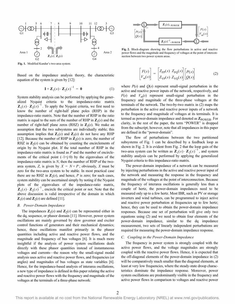
Fig. 1 shows Kundur’s two-area system used in this paper todemonstrate the impedance-based analysis of interarea oscillations[6]. As shown in Fig. 1, the system is partitioned into twosubsystems for impedance-based stability analysis; the imped-ances of the partitioned subsystems are denoted by Z1(s) andZ2(s), respectively. Bold letters are used because the impedanceresponse of a three-phase network is a two-by-two transfer matrixirrespective of the domain in which the impedance is defined [11].

1National Renewable Energy Laboratory (NREL)Golden, CO 80401, USA

Email: {Shahil.Shah, Weihang.Yan, Vahan.Gevorgian}@nrel.gov

2University of DenverDenver, CO 80208, USA

Email: Wenzhong.Gao@du.edu

This work was authored by Alliance for Sustainable Energy, LLC, the managerand operator of the National Renewable Energy Laboratory for the U.S.Department of Energy (DOE) under Contract No. DE-AC36-08GO28308.Funding provided by U.S. Department of Energy Office of Energy Efficiency andRenewable Energy Wind Energy Technologies Office. The views expressed in thearticle do not necessarily represent the views of the DOE or the U.S. Government.The U.S. Government retains and the publisher, by accepting the article for publi-cation, acknowledges that the U.S. Government retains a nonexclusive, paid-up,irrevocable, worldwide license to publish or reproduce the published form of thiswork, or allow others to do so, for U.S. Government purposes.

This report is available at no cost from the National Renewable Energy Laboratory (NREL) at www.nrel.gov/publications.1

Based on the impedance analysis theory, the characteristicequation of the system is given by [12]:

(1)

System stability analysis can be performed by applying the gener-alized Nyquist criteria to the impedance-ratio matrix

. To apply the Nyquist criteria, we first need toknow the number of right-half plane poles (RHP) in theimpedance-ratio matrix. Note that the number of RHP in the ratiomatrix is equal to the sum of the number of RHP in Z1(s) and thenumber of right-half plane zeros (RHZ) in Z2(s). We make anassumption that the two subsystems are individually stable; thisassumption implies that Z1(s) and Z2(s) do not have any RHP[12]. Because the number of RHP in Z2(s) is zero, the number ofRHZ in Z2(s) can be obtained by counting the encirclements oforigin by its Nyquist plot. If the total number of RHP in theimpedance-ratio matrix is found as P and the number of encircle-ments of the critical point (–1+j·0) by the eigenvalues of theimpedance-ratio matrix is N, then the number of RHP of the two-area system, Z, is given by ; obviously, X must bezero for the two-area system to be stable. In most practical casethere are no RHZ in Z2(s), and hence, P is zero; for such cases,system stability can be ascertained simply by noting if the Nyquistplots of the eigenvalues of the impedance-ratio matrix,

, encircle the critical point or not. Note that theabove discussion is valid irrespective of the domain in whichZ1(s) and Z2(s) are defined [11].

B. Power-Domain Impedance

The impedances Z1(s) and Z2(s) can be represented either inthe dq, sequence, or phasor domain [11]. However, power systemoscillations are mainly governed by slow governor and excitercontrol functions of generators and their mechanical dynamics;hence, these oscillations manifest primarily in the phasorquantities including active and reactive power flows, and themagnitude and frequency of bus voltages [6]. It is much moreinsightful if the analysis of power system oscillations dealsdirectly with these phasor quantities instead of instantaneousvoltages and currents—the reason why the small-signal modalanalysis uses active and reactive power flows, and frequencies (orangles) and magnitudes of bus voltages as state variables [6].Hence, for the impedance-based analysis of interarea oscillations,a new type of impedance is defined in this paper relating the activeand reactive power flows with the frequency and magnitude of thevoltages at the terminals of a three-phase network:

(2)

where P(s) and Q(s) represent small-signal perturbation in theactive and reactive power inputs of the network, respectively, andF(s) and Vm(s) represent small-signal perturbation in thefrequency and magnitude of the three-phase voltages at theterminals of the network. The two-by-two matrix in (2) maps theperturbation in the active and reactive power inputs of a networkto the frequency and magnitude of voltages at its terminals. It istermed as power-domain impedance and denoted as ZPOWER. Forclarity, in the rest of the paper, the term “POWER” is droppedfrom the subscript; however, note that all impedances in this paperare defined in the “power-domain”.

The flow of perturbations between the two partitionedsubsystems of Fig. 1 can be described by a feedback loop asshown in Fig. 2. It is evident from Fig. 2 that the loop gain of thetwo-area system can be written as , and systemstability analysis can be performed by applying the generalizedNyquist criteria to this impedance-ratio matrix.

The power-domain impedance of a network can be measuredby injecting perturbations in the active and reactive power input ofthe network and measuring the response in the frequency andmagnitude of the voltages at the point of interconnection. Becausethe frequency of interarea oscillations is generally less than acouple of hertz, the power-domain impedances need to bemeasured only up to a few hertz. Most IBR, such as PV or storageinverters and wind turbines, can be programmed to inject activeand reactive power perturbation at frequencies up to few hertz;hence, they can be used to obtain the power-domain impedanceresponses. Because one set of perturbation will give only twoequations using (2) and we need to obtain four elements of thepower-domain impedance, similar to the dq impedancemeasurement, two sets of linearly independent perturbations arerequired for measuring the power-domain impedance response.

C. Coupling in the Power-Domain Impedance

The frequency in power system is strongly coupled with theactive power flows, and the voltage magnitudes are stronglycoupled with the reactive power flows. Hence, it is expected thatthe off-diagonal elements of the power-domain impedance in (2)will be comparatively much smaller than the diagonal elements, atleast at very low frequencies, where the steady-state droop charac-teristics dominate the impedance response. Moreover, powersystem oscillations are predominantly visible in the frequency andactive power flows in comparison to voltages and reactive power

Fig. 1. Modified Kundur’s two-area system.

G1 G3

G2 G4

1 5 6 7

2

3

4

8 9 10 11 12

Area 1 Area 2Z1(s) Z2(s)

I Z1 s Z2 s 1–+ 0=

Z1 s Z2 s 1–

X N P+=

Z1 s Z2 s 1–

F s Vm s

ZFP s ZFQ s

ZVP s ZVQ s P s Q s

=

Fig. 2. Block-diagram showing the flow perturbations in active and reactivepower flows and the magnitude and frequency of voltages at the point of intercon-nection between two power system areas.

Z2(s)–1, POWER

_ Z1(s), POWER

P s Q s

F s Vm s

Z1 s Z2 s 1–

This report is available at no cost from the National Renewable Energy Laboratory (NREL) at www.nrel.gov/publications.2

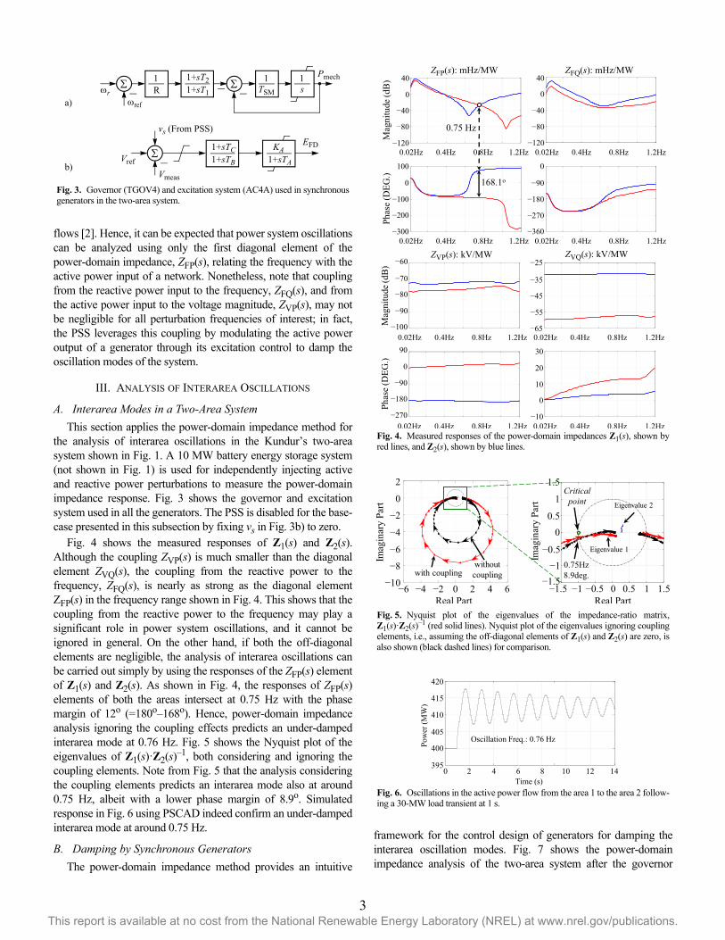
flows [2]. Hence, it can be expected that power system oscillationscan be analyzed using only the first diagonal element of thepower-domain impedance, ZFP(s), relating the frequency with theactive power input of a network. Nonetheless, note that couplingfrom the reactive power input to the frequency, ZFQ(s), and fromthe active power input to the voltage magnitude, ZVP(s), may notbe negligible for all perturbation frequencies of interest; in fact,the PSS leverages this coupling by modulating the active poweroutput of a generator through its excitation control to damp theoscillation modes of the system.

III. ANALYSIS OF INTERAREA OSCILLATIONS

A. Interarea Modes in a Two-Area System

This section applies the power-domain impedance method forthe analysis of interarea oscillations in the Kundur’s two-areasystem shown in Fig. 1. A 10 MW battery energy storage system(not shown in Fig. 1) is used for independently injecting activeand reactive power perturbations to measure the power-domainimpedance response. Fig. 3 shows the governor and excitationsystem used in all the generators. The PSS is disabled for the base-case presented in this subsection by fixing vs in Fig. 3b) to zero.

Fig. 4 shows the measured responses of Z1(s) and Z2(s).Although the coupling ZVP(s) is much smaller than the diagonalelement ZVQ(s), the coupling from the reactive power to thefrequency, ZFQ(s), is nearly as strong as the diagonal elementZFP(s) in the frequency range shown in Fig. 4. This shows that thecoupling from the reactive power to the frequency may play asignificant role in power system oscillations, and it cannot beignored in general. On the other hand, if both the off-diagonalelements are negligible, the analysis of interarea oscillations canbe carried out simply by using the responses of the ZFP(s) elementof Z1(s) and Z2(s). As shown in Fig. 4, the responses of ZFP(s)elements of both the areas intersect at 0.75 Hz with the phasemargin of 12o (=180o–168o). Hence, power-domain impedanceanalysis ignoring the coupling effects predicts an under-dampedinterarea mode at 0.76 Hz. Fig. 5 shows the Nyquist plot of theeigenvalues of Z1(s)·Z2(s)–1, both considering and ignoring thecoupling elements. Note from Fig. 5 that the analysis consideringthe coupling elements predicts an interarea mode also at around0.75 Hz, albeit with a lower phase margin of 8.9o. Simulatedresponse in Fig. 6 using PSCAD indeed confirm an under-dampedinterarea mode at around 0.75 Hz.

B. Damping by Synchronous Generators

The power-domain impedance method provides an intuitive

framework for the control design of generators for damping theinterarea oscillation modes. Fig. 7 shows the power-domainimpedance analysis of the two-area system after the governor

Fig. 3. Governor (TGOV4) and excitation system (AC4A) used in synchronousgenerators in the two-area system.

rref

1R

1+sT21+sT1_ _

1TSM

_ 1s

Pmech

a)

_Vref

Vmeas

vs (From PSS)

1+sTC1+sTB

KA1+sTA

EFD

b)

40

70

60

80

90

0

90

90

180

270

100

0.02Hz 0.4Hz 0.8Hz 1.2Hz

0.02Hz 0.4Hz 0.8Hz 1.2Hz

Mag

nit

ude

(dB

)P

has

e (D

EG

.)

0.02Hz 0.4Hz 0.8Hz 1.2Hz

0.02Hz 0.4Hz 0.8Hz 1.2Hz

40

0 0

40

40

80

120

0

100

100

200

300

0

180

360

80

120

270

Mag

nit

ude

(dB

)P

has

e (D

EG

.)

0.02Hz 0.4Hz 0.8Hz 1.2Hz

0.02Hz 0.4Hz 0.8Hz 1.2Hz

0.02Hz 0.4Hz 0.8Hz 1.2Hz

0.02Hz 0.4Hz 0.8Hz 1.2Hz

35

25

45

65

55

20

30

10

0

10

90

0.76Hz

168.1o

Fig. 4. Measured responses of the power-domain impedances Z1(s), shown byred lines, and Z2(s), shown by blue lines.

ZFP(s): mHz/MW ZFQ(s): mHz/MW

ZVQ(s): kV/MWZVP(s): kV/MW

0.75 Hz

Fig. 5. Nyquist plot of the eigenvalues of the impedance-ratio matrix,Z1(s)·Z2(s)–1 (red solid lines). Nyquist plot of the eigenvalues ignoring couplingelements, i.e., assuming the off-diagonal elements of Z1(s) and Z2(s) are zero, isalso shown (black dashed lines) for comparison.

Criticalpoint

0.75Hz

8.9deg.

Eigenvalue 2

Real Part

Imag

inar

y P

art

1.510.500.51

1.5

1

0.5

0

0.5

1

0 2 4 6246

0

2

4

6

8

10

2

with couplingwithout

coupling

1.51.5

Eigenvalue 1

Real Part

Imag

inar

y P

art

Fig. 6. Oscillations in the active power flow from the area 1 to the area 2 follow-ing a 30-MW load transient at 1 s.

Oscillation Freq.: 0.76 Hz

Time (s)

Pow

er (

MW

)

0 2 4 6 8 10 12 14

400

395

405

410

415

420

This report is available at no cost from the National Renewable Energy Laboratory (NREL) at www.nrel.gov/publications.3

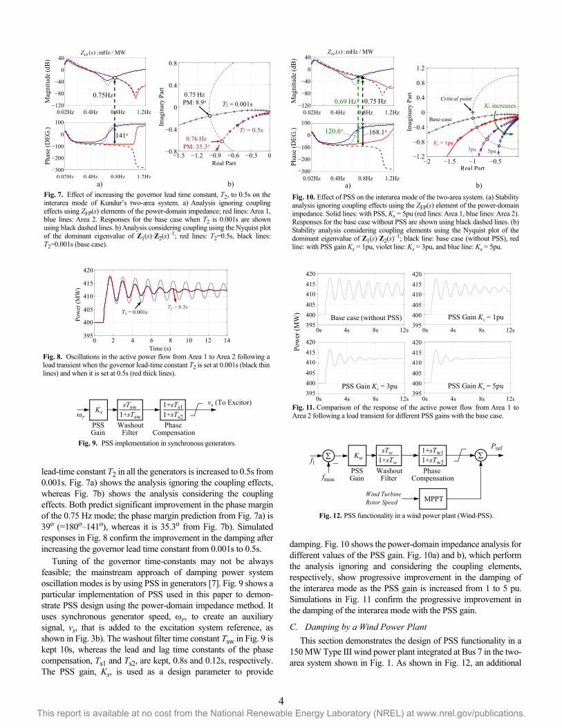
lead-time constant T2 in all the generators is increased to 0.5s from0.001s. Fig. 7a) shows the analysis ignoring the coupling effects,whereas Fig. 7b) shows the analysis considering the couplingeffects. Both predict significant improvement in the phase marginof the 0.75 Hz mode; the phase margin prediction from Fig. 7a) is39o (=180o–141o), whereas it is 35.3o from Fig. 7b). Simulatedresponses in Fig. 8 confirm the improvement in the damping afterincreasing the governor lead time constant from 0.001s to 0.5s.

Tuning of the governor time-constants may not be alwaysfeasible; the mainstream approach of damping power systemoscillation modes is by using PSS in generators [7]. Fig. 9 shows aparticular implementation of PSS used in this paper to demon-strate PSS design using the power-domain impedance method. Ituses synchronous generator speed, r, to create an auxiliarysignal, vs, that is added to the excitation system reference, asshown in Fig. 3b). The washout filter time constant Tsw in Fig. 9 iskept 10s, whereas the lead and lag time constants of the phasecompensation, Ts1 and Ts2, are kept, 0.8s and 0.12s, respectively.The PSS gain, Ks, is used as a design parameter to provide

damping. Fig. 10 shows the power-domain impedance analysis fordifferent values of the PSS gain. Fig. 10a) and b), which performthe analysis ignoring and considering the coupling elements,respectively, show progressive improvement in the damping ofthe interarea mode as the PSS gain is increased from 1 to 5 pu.Simulations in Fig. 11 confirm the progressive improvement inthe damping of the interarea mode with the PSS gain.

C. Damping by a Wind Power Plant

This section demonstrates the design of PSS functionality in a150 MW Type III wind power plant integrated at Bus 7 in the two-area system shown in Fig. 1. As shown in Fig. 12, an additional

0.02Hz 0.4Hz 0.8Hz 1.2Hz

0.02Hz 0.4Hz 0.8Hz 1.2Hz

Mag

nit

ude

(dB

)P

has

e (D

EG

.)

40

0

0

100

100

200

300

40

80

120

FP ( ) : mHz / MWZ s

0.75Hz

141o

Real PartIm

agin

ary P

art

T2 = 0.5s

0.3 00.60.91.21.50.8

0.4

0

0.4

0.8

0.76 Hz

PM: 35.3o

T2 = 0.001s

0.75 Hz

PM: 8.9o

Fig. 7. Effect of increasing the governor lead time constant, T2, to 0.5s on theinterarea mode of Kundur’s two-area system. a) Analysis ignoring couplingeffects using ZFP(s) elements of the power-domain impedance; red lines: Area 1,blue lines: Area 2. Responses for the base case when T2 is 0.001s are shownusing black dashed lines. b) Analysis considering coupling using the Nyquist plotof the dominant eigenvalue of Z1(s)·Z2(s)–1; red lines: T2=0.5s, black lines:T2=0.001s (base case).

a) b)

Time (s)

Pow

er (

MW

)

0 2 4 6 8 10 12 14

400

395

405

410

415

420

T2 = 0.5sT2 = 0.001s

Fig. 8. Oscillations in the active power flow from Area 1 to Area 2 following aload transient when the governor lead-time constant T2 is set at 0.001s (black thinlines) and when it is set at 0.5s (red thick lines).

1+sTs2

Fig. 9. PSS implementation in synchronous generators.

rKs

sTsw1+sTsw

vs (To Excitor)1+sTs1

WashoutFilter

PSSGain

PhaseCompensation

0.02Hz 0.4Hz 0.8Hz 1.2Hz

0.02Hz 0.4Hz 0.8Hz 1.2Hz

Mag

nit

ude

(dB

)P

has

e (D

EG

.)

40

0

0

100

100

200

300

40

80

120

FP ( ) : mHz / MWZ s

0.69 Hz

120.6o 168.1o

0.75 Hz

0Real Part

Imag

inar

y P

art

1.22 1.5 1 0.5

0.8

0.4

0

0.4

0.8

1.2

Ks increasesCritical point

Base-case

Ks = 1pu3pu 5pu

Fig. 10. Effect of PSS on the interarea mode of the two-area system. (a) Stabilityanalysis ignoring coupling effects using the ZFP(s) element of the power-domainimpedance. Solid lines: with PSS, Ks = 5pu (red lines: Area 1, blue lines: Area 2).Responses for the base case without PSS are shown using black dashed lines. (b)Stability analysis considering coupling elements using the Nyquist plot of thedominant eigenvalue of Z1(s)·Z2(s)–1; black line: base case (without PSS), redline: with PSS gain Ks = 1pu, violet line: Ks = 3pu, and blue line: Ks = 5pu.

a) b)

0s 4s 8s 12s

0s 4s 8s 12s

Pow

er (

MW

)

0s 4s 8s 12s

0s 4s 8s 12s

420

415

410

405

400

395

420

415

410

405

400

395

420

415

410

405

400

395

420

415

410

405

400

395

Base case (without PSS) PSS Gain Ks = 1pu

PSS Gain Ks = 5puPSS Gain Ks = 3pu

Fig. 11. Comparison of the response of the active power flow from Area 1 toArea 2 following a load transient for different PSS gains with the base case.

1+sTw2

Fig. 12. PSS functionality in a wind power plant (Wind-PSS).

KwsTw

1+sTw

Pref 1+sTw1

WashoutFilter

PSSGain

PhaseCompensation

f1 _

fmeas

MPPTWind TurbineRotor Speed

This report is available at no cost from the National Renewable Energy Laboratory (NREL) at www.nrel.gov/publications.4

power control loop is added in the wind turbines in parallel withthe MPPT loop to modulate the active power output of the windpower plant depending on the error between the nominalfrequency, f1, and the frequency measurement at the point ofcommon coupling, fmeas. The power-domain impedance-basedanalysis of the system with and without the PSS functionality inthe wind power plant is shown in Fig. 13; the analysis predictssignificant improvement in the phase margin of the interarea modeafter the installation of Wind-PSS in the wind power plant. Thesimulated responses in Fig. 14 confirm the improvement in thedamping of the interarea mode using Wind-PSS. Note from Fig.14b) how the wind power plant modulates its active power outputafter a transient transmission line fault to quickly damp the

interarea oscillations.

IV. CONCLUSIONS

Because of the use of non-standardized controls by IBR andunavailability of their dynamic models, new impedance-basedtools are necessary for the stability analysis of modern powersystems. The power-domain impedance theory presented in thispaper can evaluate power system oscillations without dependingon the analytical model of the system. Power-domain impedanceresponses can be measured at different points in the system usingsimulation models of the system or actual measurements. Thepower-domain impedance responses can be used both forpredicting the power system oscillation modes as well as fordesigning damping controls in conventional generators andmodern IBR including wind and PV power plants and inverter-interfaced energy storage systems. The online measurement of thepower-domain impedance responses can also support the real-timemonitoring of the power system frequency response [13] inaddition to the power system oscillation modes.

REFERENCES

[1] M. Singh, A. J. Allen, E. Muljadi, V. Gevorgian, Y. Zhang, and S.Santoso, “Interarea oscillation damping controls for wind power plants,”IEEE Trans. Sustain. Energy, vol. 6, no. 3, pp. 967-975, July 2015.

[2] L. Wu, S. You, X. Zhang, Y. Cui, Y. Liu, and Y. Liu, “Statistical analysisof the FNET/GridEye-detected inter-area oscillations in easter intercon-nection (EI),” in Proc. 2017 Power and Energy Soc. Gen. Meeting,Chicago, IL.

[3] “Oscillation Event 03.12.2017 – System Protection and Dynamics WG,”ENTSO-E, Brussels, Belgium, 2018.

[4] F. R. Schleif and J. H. White, “Damping for the northwest – southwestoscillations—an analog study,” IEEE Trans. Power App. and Syst., vol.85, no. 12, pp. 1239-1247, Dec. 1966.

[5] W. Mo, Y. Chen, H. Chen, Y. Liu, Y. Zhong, J. Hou, Q. Gao, and C. Li,“Analysis and measures of ultralow-frequency oscillations in a large-scale hydropower transmission system,” IEEE. J. Emerg. Sel. TopicsPower Electron., vol. 6, no. 3, pp. 1077-1085, Se. 2018.

[6] P. Kundur, Power System Stability and Control. McGraw-Hill, 1994.[7] F. P. Demello and C. Concordia, “Concepts of synchronous machine

stability as affected excitation control,” IEEE Trans. Power App. andSyst., vol. 88, no. 4, pp. 316-329, April 1969.

[8] E. Rehman, M. Miller, J. Schmall, S. H. Huang, “Dynamic stabilityassessment of high penetration of renewable generation in the ERCOTgrid,” ERCOT, Taylor, TX, USA, 2018. [Online]. http://www.ercot.com/content/wcm/lists/144927/Dynamic_Stability_Assesment_of_High_Pen-etration_of_ Renewable_Generation.pdf

[9] E. Rehman, M. G. Miller, J. Schmall, S. H. Huang, and J. Billo, “Stabilityassessment of high penetration of inverter-based generation in theERCOT grid,” in Proc. 2019 IEEE Power and Energy Soc. Gen. Meeting,Atlanta, GA.

[10] J. F. Hauer, “Application of prny analsysi to the determination of modalcontent and equivalent modesl for measured power system responses,”IEEE Trans. Power Syst., vol. 6, no. 3, pp. 1062-1068, Aug. 1991.

[11] S. Shah and L. Parsa, “Impedance modeling of three-phase voltage sourceconverters in DQ, sequence, and phasor domains,” IEEE Trans. EnergyConv., vol. 32, no. 3, pp. 1139-1150, April 2017.

[12] S. Shah, “Small and large signal impedance modeling for stabilityanalysis of grid-connected voltage source converters,” Ph.D. dissertation,Dept. Elect. Eng., Rensselaer Polytechnic Institute, Troy, NY, 2018.

[13] S. Shah and V. Gevorgian, “Impedance-based characterization of powersystem frequency response,” in Proc. 2019 Power and Energy Soc. Gen.Meeting (PESGM), Atlanta, GA.

0.66 Hz

PM: 16.2o

with Wind-PSS

Base-

case

Real Part

Imag

inar

y P

art

0.65 Hz

PM: 45.4o

0.5 0 0.5 1.0 1.51.01.51.5

1.0

0.5

0.5

1.0

1.5

00.02Hz 0.4Hz 0.8Hz 1.2Hz

0.02Hz 0.4Hz 0.8Hz 1.2Hz

0.65Hz

130.2o

40

0

50

100

0

100

40

80

120

Mag

nit

ude

(dB

)P

has

e (D

EG

.)

50

Fig. 13. Damping of the interarea mode by implementing PSS functionality in awind power plant connected at Bus 7 in the two-area system. (a) Stability analy-sis ignoring coupling effects using the ZFP(s) element of the power-domainimpedance. Solid lines: with Wind-PSS (red lines: Area 1, blue lines: Area 2).Responses for the base case without Wind-PSS are shown using black dashedlines. (b) Analysis using the Nyquist plot of the dominant eigenvalue ofZ1(s)·Z2(s)–1; black line: base case (without Wind-PSS), red line: with Wind-PSS.

a) b)

ZFP(s): mHz/MW

Time (s)

Pow

er (

MW

)

0 5 10 15 20 2580

100

120

140

160

Wind farm output

with Wind-PSS

Wind farm output

without Wind-PSS

Time (s)

Pow

er (

MW

)

0 5 10 15 20 25390

410

430

450

470

Without Wind-PSS

With Wind-PSS

Fig. 14. Simulated responses following a transient fault event with and withoutPSS functionality by the wind power plant. a) active power flow from Area 1 toArea 2, and b) power output of the wind power plant.

a)

b)

This report is available at no cost from the National Renewable Energy Laboratory (NREL) at www.nrel.gov/publications.5