populations and samples central limit theorem. lecture objectives you should be able to: 1.define...
TRANSCRIPT

Populations and Samples
Central Limit Theorem

Lecture Objectives
You should be able to:
1. Define the Central Limit Theorem
2. Explain in your own words the relationship between a population distribution and the distribution of the sample means.
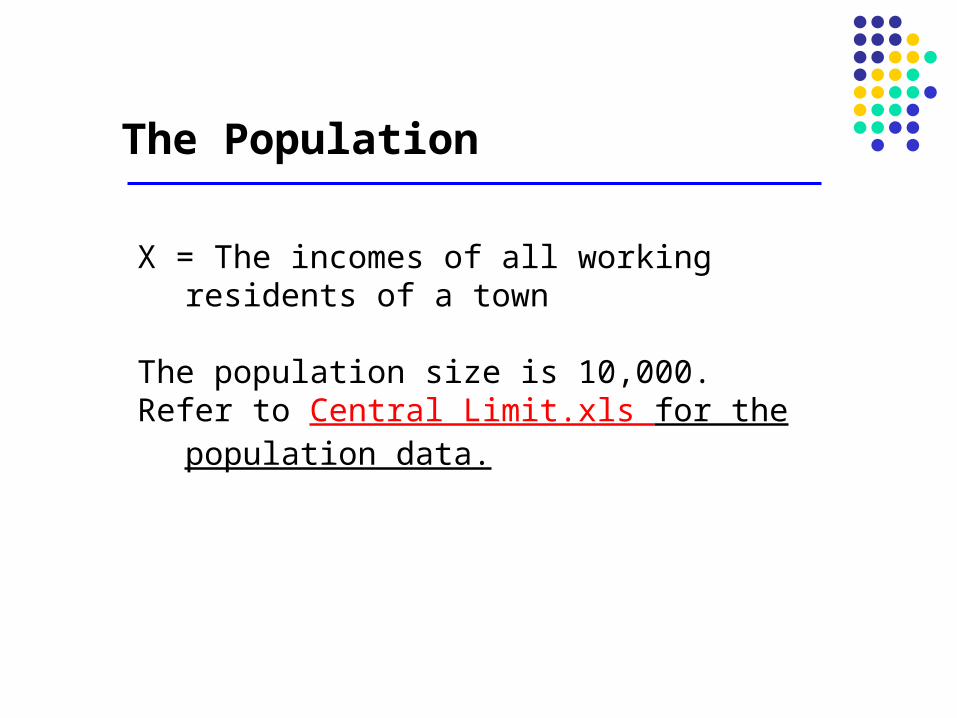
The Population
X = The incomes of all working residents of a town
The population size is 10,000. Refer to Central Limit.xls for the population data.

Population Distribution
Histogram of Population Data
0100200300400500600700800900
10001100
1000
0
2000
0
3000
0
4000
0
5000
0
6000
0
7000
0
8000
0
9000
0
Mor
e
Income up to the given number ($)
Fre
qu
ency
Mean $50,185.85
Stdevp $28,772.27
Note that the distribution is uniform, not normal
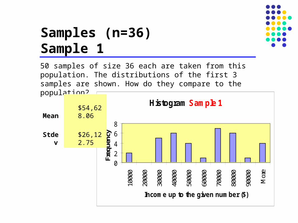
Samples (n=36) Sample 1
Histogram Sample 1
024
68
1000
0
2000
0
3000
0
4000
0
5000
0
6000
0
7000
0
8000
0
9000
0
Mor
e
Income up to the given number ($)
Freq
uenc
y
50 samples of size 36 each are taken from this population. The distributions of the first 3 samples are shown. How do they compare to the population?
Mean $54,628.06
Stdev $26,122.75

Histogram Sample 2
0
2
4
6
810
000
2000
0
3000
0
4000
0
5000
0
6000
0
7000
0
8000
0
9000
0
Mor
e
Bin
Fre
qu
ency
Sample 2
Mean $41,987.92
Stdev $27,950.33
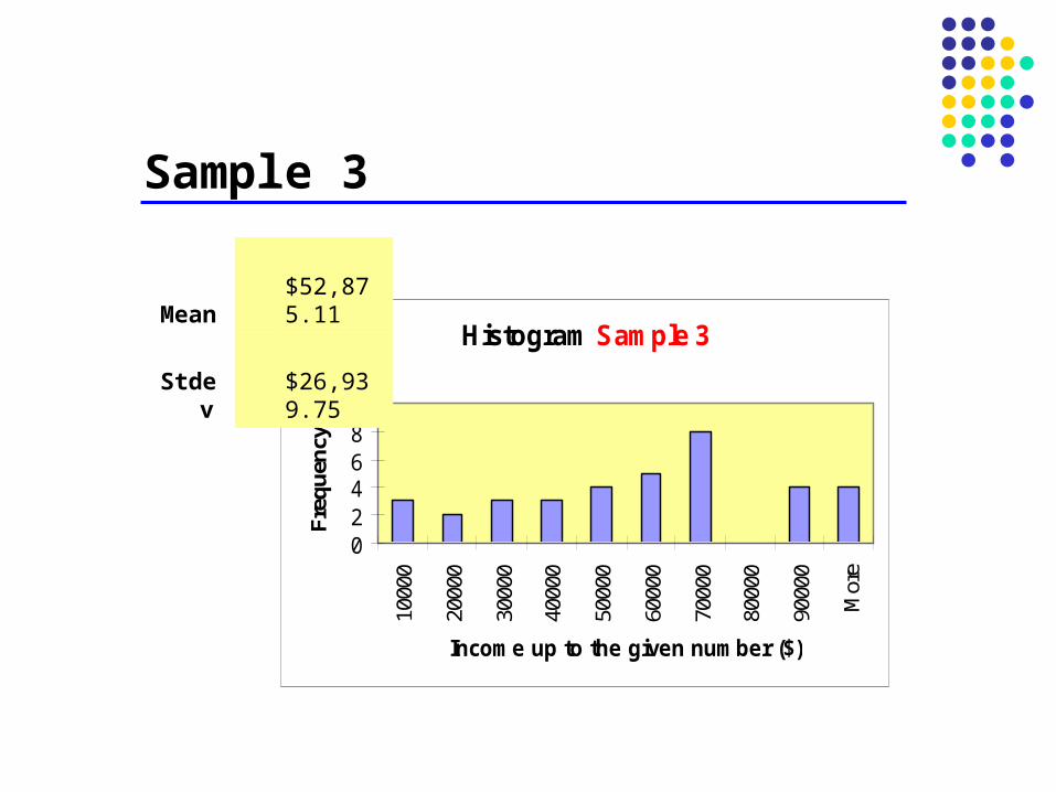
Sample 3
Histogram Sample 3
02468
1010
000
2000
0
3000
0
4000
0
5000
0
6000
0
7000
0
8000
0
9000
0
Mor
e
Income up to the given number ($)
Fre
qu
ency
Mean $52,875.11
Stdev $26,939.75
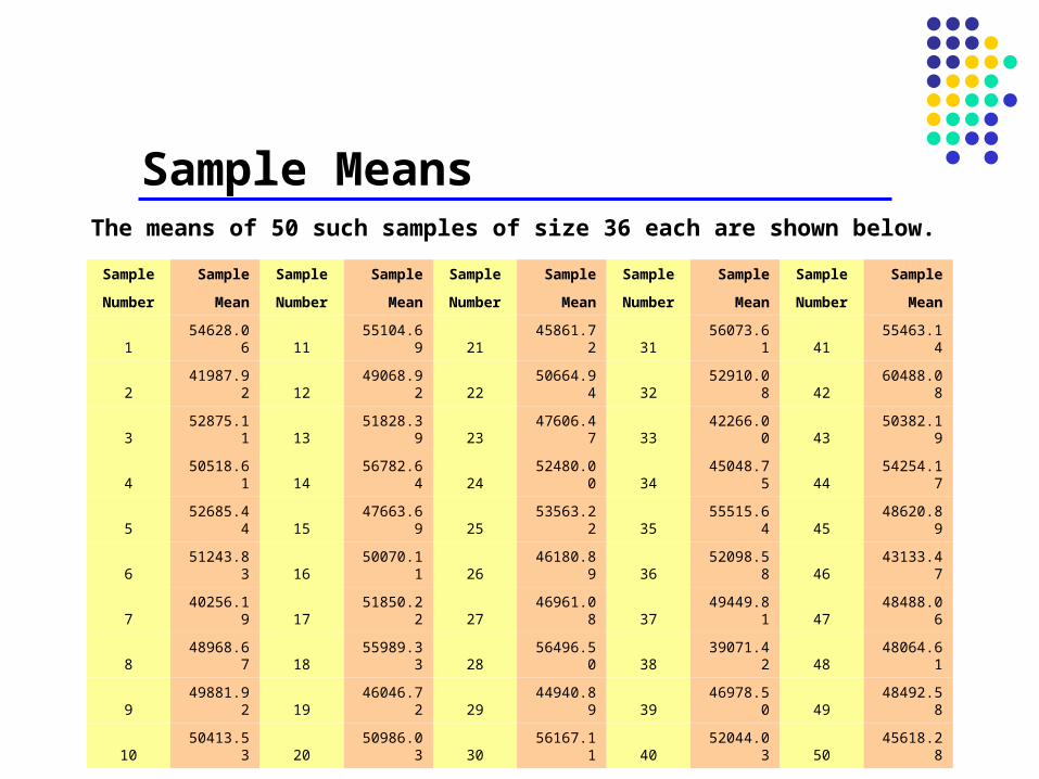
Sample Means
Sample Sample Sample Sample Sample Sample Sample Sample Sample Sample
Number Mean Number Mean Number Mean Number Mean Number Mean
1 54628.06 11 55104.69 21 45861.72 31 56073.61 41 55463.14
2 41987.92 12 49068.92 22 50664.94 32 52910.08 42 60488.08
3 52875.11 13 51828.39 23 47606.47 33 42266.00 43 50382.19
4 50518.61 14 56782.64 24 52480.00 34 45048.75 44 54254.17
5 52685.44 15 47663.69 25 53563.22 35 55515.64 45 48620.89
6 51243.83 16 50070.11 26 46180.89 36 52098.58 46 43133.47
7 40256.19 17 51850.22 27 46961.08 37 49449.81 47 48488.06
8 48968.67 18 55989.33 28 56496.50 38 39071.42 48 48064.61
9 49881.92 19 46046.72 29 44940.89 39 46978.50 49 48492.58
10 50413.53 20 50986.03 30 56167.11 40 52044.03 50 45618.28
The means of 50 such samples of size 36 each are shown below.

Distribution of Sample Means
Distribution of the Sample Means50 samples of size 36 each
02468
1012141618
40000.0
0
44000.0
0
48000.0
0
52000.0
0
56000.0
0
60000.0
0
More
Sample Means
Fre
qu
en
cy
Mean 50084.70
Stdev 4607.82

Population Mean = = 50,185.85Mean of Sample Means = = 50,084.70
Population Standard Deviation = = 28,772.27Standard Deviation of Sample Means = = 4,607.82(also called Standard Error, or SE)
(Pop. Standard Deviation) / SE = 6.24
Sample size (n) = 36Square root of sample size √n = 6
Population and Sampling Means
x
x

Central Limit Theorem
x
Regardless of the population distribution, the distribution of the sample means is approximately normal for sufficiently large sample sizes (n>=30), with
and
nx

Questions
1. How will the distribution of sample means change if • the sample size goes up to n=100?• the sample size goes down to n=2?
2. Is the distribution of a single sample the same as the distribution of the sample means?
3. If a population mean = 100, and pop. standard deviation = 24, and we take all possible samples of size 64, the mean of the sampling distribution (sample means) is _______ and the standard deviation of the sampling distribution is _______.

Applying the results
If the sample means are normally distributed, what proportion of them are within ± 1 Standard
Error? what proportion of them are within ± 2 Standard
Errors?
If you take just one sample from a population, how likely is it that its mean will be within 2 SEs of the population mean?
How likely is it that the population mean is within 2 SEs of your sample mean?

The population mean is within 2 SEs of the sample mean, 95% of the time.
Thus , is in the range defined by:
2*SE, about 95% of the time.
(2 *SE) is also called the Margin of Error (MOE).
95% is called the confidence level.
Confidence Intervals
x