random max sat, random max cut and their phase transitionshajiagha/max.pdf · random max sat,...
TRANSCRIPT
Random max sat, Random max cut,
and Their Phase Transitions
Don Coppersmith∗ David Gamarnik∗
Mohammad T. Hajiaghayi† Gregory B. Sorkin∗
Abstract
With random inputs, certain decision problems undergo a “phasetransition”. We prove similar behavior in an optimization context.
Given a conjunctive normal form (CNF) formula F on n variablesand with m k-variable clauses, denote by max F the maximum numberof clauses satisfiable by a single assignment of the variables. (Thusthe decision problem k-sat is to determine if max F is equal to m.)With the formula F chosen at random, the expectation of max F istrivially bounded by 3
4m 6 E max F 6 m. We prove that for random
formulas with m = bcnc clauses: for constants c < 1, E max F isbcnc − Θ(1/n); for large c, it approaches ( 3
4c + Θ(
√c))n; and in the
“window” c = 1 + Θ(n−1/3), it is cn−Θ(1). Our full results are moredetailed, but this already shows that the optimization problem max
2-sat undergoes a phase transition just as the 2-sat decision problemdoes, and at the same critical value c = 1. Most of our results areestablished without reference to the analogous propositions for decision2-sat, and can be used to reproduce them.
We consider “online” versions of max 2-sat, and show that forone version the obvious greedy algorithm is optimal; all other naturalquestions remain open.
We can extend only our simplest max 2-sat results to max k-sat, but we conjecture a “max k-sat limiting function conjecture”analogous to the folklore “satisfiability threshold conjecture”, but openeven for k = 2. Neither conjecture immediately implies the other, butit is natural to further conjecture a connection between them.
We also prove analogous results for random max cut.
∗Department of Mathematical Sciences, IBM T.J. Watson Research Center, Yorktown
Heights NY 10598, USA. e-mail copper,gamarnik,[email protected]†Department of Mathematics, M.I.T., Cambridge MA 02139, USA.
e-mail [email protected]
1

Contents
1 Introduction 31.1 Outlook . . . . . . . . . . . . . . . . . . . . . . . . . . . . . . 31.2 Motivations . . . . . . . . . . . . . . . . . . . . . . . . . . . . 41.3 Problem: Random MAX CSP . . . . . . . . . . . . . . . . . . 51.4 Related work . . . . . . . . . . . . . . . . . . . . . . . . . . . 6
2 Model, notation, and inequalities 7
3 Summary of MAX 2-SAT results 8
4 Random MAX 2-SAT 114.1 Sub-critical MAX 2-SAT . . . . . . . . . . . . . . . . . . . . . 114.2 High-density random MAX 2-SAT . . . . . . . . . . . . . . . 144.3 Low-density random MAX 2-SAT . . . . . . . . . . . . . . . . 18
5 The MAX 2-SAT scaling window 225.1 Case c = 1 + λn−1/3 , λ 6 −1 . . . . . . . . . . . . . . . . . . 235.2 Case c = 1 + λn−1/3 , λ > 1 . . . . . . . . . . . . . . . . . . . 26
5.2.1 Useful facts . . . . . . . . . . . . . . . . . . . . . . . . 285.2.2 Phase I . . . . . . . . . . . . . . . . . . . . . . . . . . 295.2.3 Phase II . . . . . . . . . . . . . . . . . . . . . . . . . . 335.2.4 Phases I, II and III . . . . . . . . . . . . . . . . . . . . 355.2.5 Remarks . . . . . . . . . . . . . . . . . . . . . . . . . . 35
6 Random MAX k-SAT and MAX CSP 376.1 Concentration and limits . . . . . . . . . . . . . . . . . . . . . 376.2 High-density MAX k-SAT and MAX CSP . . . . . . . . . . . 38
7 Online random MAX 2-SAT 40
8 Random MAX CUT 438.1 Motivation . . . . . . . . . . . . . . . . . . . . . . . . . . . . 438.2 MAX CUT . . . . . . . . . . . . . . . . . . . . . . . . . . . . 458.3 Results . . . . . . . . . . . . . . . . . . . . . . . . . . . . . . . 468.4 Subcritical MAX CUT . . . . . . . . . . . . . . . . . . . . . . 478.5 High-density random MAX CUT . . . . . . . . . . . . . . . . 488.6 Low-density random MAX CUT . . . . . . . . . . . . . . . . 488.7 Scaling window . . . . . . . . . . . . . . . . . . . . . . . . . . 50
2
9 Conclusions and open problems 52
1 Introduction
In this paper, we consider random instances of max 2-sat, max k-sat, andmax cut. Just as random instances of the decision problem 2-sat show aphase transition from almost-sure satisfiability to almost-sure unsatisfiabilityas the instance “density” increases above 1, so the maximization problemshows a transition at the same point, with the expected number of clausesnot satisfied by an optimal solution quickly changing from Θ(1/n) to Θ(n).Max cut experiences a similar phase transition: as a random graph’s edgedensity crosses above 1/n, the number of edges not cut in an optimal cutchanges from Θ(1) to Θ(n).
Our methods are well established ones: the first-moment method for up-per bounds; algorithmic analysis including the differential-equation methodfor lower bounds; and some more sophisticated martingale arguments forthe analysis of the scaling window. The interest of the work lies in therelative straightforwardness of the methods, as well as in the results. Thequestions we ask seem very natural, and the answers obtained for max 2-
sat and max cut are happily neat, and, with one notable exception, fairlycomprehensive.
A preliminary version of this paper appeared as [CGHS03].
1.1 Outlook
Beyond our particular results for max 2-sat and max cut, we hope tospark further work on phase transitions in random instances of optimiza-tion problems generally, in particular of max csps (constraint satisfactionproblems). Random instances of optimization problems have been studiedextensively — some that come to mind are the travelling salesman problem,minimum spanning tree, minimum assignment, minimum bisection, mini-mum coloring, and maximum clique — but little has been said about phasetransitions in such cases, and indeed many of the examples do not even havea natural parameter whose continuous variation could give rise to a phasetransition.
Many problems, including all csps, have natural decision and optimiza-tion versions: one can ask whether a graph is k-colorable, or ask for theminimum number of colors it requires. We suggest that in a random setting,the optimization version is quite as interesting as the decision version. Fur-thermore, optimization problems may plausibly be easier to analyze than
3
decision problems because the quantities of interest vary more smoothly.In fact, a recent triumph in the analysis of a decision problem, Bollobas,Borgs, Chayes, Kim, and Wilson’s characterization of the “scaling window”for 2-sat, used as a smoothed quantity the size of the “spine” of a for-mula [BBC+01]. A way to view our max 2-sat results is that instead oftaking the size of the spine as our “order parameter”, we take the size of amaximum satisfiable subformula. This seems comparably tractable (we re-produce the result of [BBC+01] incompletely, but more easily), and arguablymore natural. Generally, when a decision problem has an optimization ana-log, the value of the optimum is both interesting in its own right, and, wesuggest, an obvious candidate order parameter for studying the decisionproblem.
1.2 Motivations
Let F be a k-sat formula with n variables X1, . . . , Xn . An “assignment” ofthese variables consists of setting each Xi to either 1 (True) or 0 (False); wemay write an assignment as a vector ~X ∈ 0, 1n . k-sat is well understood.In particular, it is a canonical NP-hard problem to determine if a givenformula F is satisfiable or not, except for k = 2 when this decision problemis solvable in essentially linear time.
Random instances of k-sat have recently received wide attention. LetF(n, m) denote the set of all formulas with n variables and m clauses, whereeach clause is proper (consisting of k distinct variables, each of which may becomplemented or not), and clauses may be repeated. Let F ∈ F be chosenuniformly at random; this is equivalent to choosing m clauses uniformly atrandom, with replacement, from the 2k
(
nk
)
possible clauses.The model is generally parametrized as F ∈ F(n, cn) for various “den-
sities” c, and the state of knowledge is summarized thus. The 2-sat caseis well understood: for c < 1, F is a.a.s. satisfiable (asymptotically al-most surely in the limit n → ∞), and for c > 1, F is a.a.s. unsatisfiable[CR92, Goe96, FdlV92]. The “scaling window” c = 1±Θ(n−1/3) has recentlybeen analyzed [BBC+01]. For k-sat, much less is known. For 3-sat, forinstance, it is known that for c < 3.42, F is a.a.s. satisfiable [KKL02] and forc > 4.6, F is a.a.s. unsatisfiable [JSV00]. (A bound of 4.506 by Boufkhad,Dubois and Mandler was announced in a 2-page abstract [DBM00], but afull version has so far appeared only as a technical report [DBM03].) It isonly conjectured, though, that for k = 3 (and for all k) the situation issimilar to that for k = 2.
4

Conjecture 1 (Satisfiability Threshold Conjecture) For each k thereexists a threshold density ck , such that for any positive ε, for all c < ck− ε,a random formula F is a.a.s. satisfiable, and for all c > ck + ε, F is a.a.s.unsatisfiable.
For large values of k, although the question of a threshold remains open,satisfiability and unsatisfiability density bounds are asymptotically equal, asshown by an analysis in [AM02] and refined in [AP03]. The closest result tothe satisfiability conjecture is a theorem of Friedgut [Fri99] proving similarthresholds, but leaving open the possibility that (for a given k), each n mayhave its own threshold ck(n), and that these may not converge to a limit.
Theorem 2 (Friedgut) For each k there exists a threshold density func-tion ck(n), such that for any positive ε, as n → ∞, for all c < ck − ε, arandom formula F is a.a.s. satisfiable, and for all c > ck + ε, F is a.a.s.unsatisfiable.
Having briefly surveyed random k-sat, let us similarly consider max k-sat. For a given formula F , let F ( ~X) be the number of clauses satisfiedby ~X . The problem max 2-sat asks for max F
.= max ~X F ( ~X), i.e., the
maximum, over all assignments ~X , of the size (number of clauses) of amaximum satisfiable subformula of F .
In the maximization setting, even 2-sat is interesting. max 2-sat isNP-hard to solve exactly, and it is even NP-hard to approximate max F towithin a factor of 21/22 [Has97]. On the other hand, a 3/4-approximationis trivial: a random assignment satisfies an expected 3/4ths of the clauses,and a derandomized algorithm is simple (our algorithm used to prove thelower bound for Theorem 5 can serve). The best known approximation ratioachievable in polynomial time is 0.940 [LLZ02]. For arbitrary 3-sat formulasF , in polynomial time, max F can be approximated to within a factor of7/8 [KZ97], but no better (unless P=NP) [Has97].
1.3 Problem: Random MAX CSP
Although both randomized and maximization versions of k-sat are thus wellstudied, we are aware of limited prior work on random max sat and otherrandom max or min constraint satisfaction problems (csps). Indeed, in theconclusions to his survey article [FdlV01] on random instances of (decision)2-sat, Fernandez de la Vega notes that nothing is known about randommax 2-sat, “which is also certainly challenging and perhaps not hopeless.”
Such questions prove to have elegant answers: we will show for examplethat random max 2-sat has a phase structure analogous to the decision
5

problem’s. We hope that maximization problems may even help in under-standing the decision problems. For 2-sat this hope is borne out to a degreeby our Theorem 7 on the scaling window of max 2-sat: using max F as anorder parameter, instead of the “spine” devised by [BBC+01], allows us toreproduce part of their result on the scaling window for decision 2-sat.
For random max cut, we obtain results which are slightly more com-prehensive than those for 2-sat, and largely though not entirely analogous.While our results for k-sat (k > 2) and other csps are very limited (seeTheorems 15 and 16), Conjectures 12 and 14 link the open questions forthe maximization and decision thresholds for random satisfiability. At thispoint we cannot guess the comparative difficulties of resolving the satisfia-bility threshold conjecture, its maximization analog, or the conjectured linkbetween them.
1.4 Related work
For a random graph, the maximum bisection and maximum cut are nearlyequivalent, and these problems have received the most and earliest attention.Bertoni, Campadelli, and Posenato in 1997 determined an upper bound onthe expected maximum bisection width for random graphs with averagedegree c [BCP97], and Verhoeven in an unpublished manuscript apparentlydating from 2000 found a lower bound as well [Ver00]. Our Theorem 20 issimply a statement of these two results, with brief proofs included for thesake of completeness.
Subsequent to our work, in 2003 this theorem was generalized to max
k-cut by Moore, Coja-Oghlan, and Sanwalini [COMS03], as part of aproject of analyzing the performance of a semi-definite programming (SDP)relaxation-based algorithm for max k-cut on random graphs G(n, c/n),focusing on asymptotically large value of c. This line of work (SDP-based approximation algorithms, starting with Goemans and Williamson’s[GW95],copy and their connections with the eigenvalues of random matrices,see for example Friedman, Kahn, and Szemeredi’s [FKS89] and Friedman’s[Fri02]) is interesting from our perspective for the possibility that it coulddetermine the exact constant of
√c on which Theorem 20 gives upper and
lower bounds.On this theme, concurrently with our work, Dıaz, Do, Serna and
Wormald derived narrow bounds for, but not quite the exact values of, thesize of optimum bisections of random cubic and 4-regular graphs [DDSW03];these problem are close kin to the maximum cut of a random graph with cnedges, c = 3/2 and c = 2 respectively.
6

Despite this attention to random max cut, we are not aware of any priortreatment of the phase transition, which occurs around average degree 1; infact prior consideration seems to have been limited to above-threshold oreven asymptotically large fixed or average degree.
For random max 2-sat, we are not aware of any prior work at all,let alone on the phase transition. These problems seem very natural, andanswers to even the simplest questions are not obvious at first blush: Fora random 2-sat formula F (n, cn) with c > 1, which is a.a.s. unsatisfiable,can we perhaps w.h.p. satisfy all but a single clause?
Our study of random max 2-sat and random max cut was also moti-vated by recent work on “avoiding a giant component”; we will discuss thisin section 8.
2 Model, notation, and inequalities
We write F (n, m) to denote a random 2-sat formula on n variables, with mclauses chosen uniformly at random with replacement from the collection ofall 22
(
n2
)
proper two-variable clauses. Typically we will fix a constant c andconsider F (n, bcnc); where it does not matter we will often write cn in lieuof bcnc and we often omit the notation b·c in other instances too. For anyformula F , define max F to be the size of a largest satisfiable subformulaof F . Our focus is the functional behavior of max F , and accordingly wedefine
f(n, m).= E max F (n, m).
We use the symbol “.=” to denote equality by definition. Throughout the
paper we reserve n, m, and c for these roles.In the context of graphs instead of formulas, we write G(n, m) for a
random graph on n vertices with m edges. For any graph G, let ~X de-scribe a partition of the vertices, and let cut(G, ~X) be the number of edgeshaving one vertex in each part of the partition. Define max cut(G)
.=
max ~X cut(G, ~X), and fcut(n, m).= E(max cut(G(n, m))).
We use standard asymptotic and “order” notation, so for example f(n) 'g(n) means f(n)/g(n) → 1 as n →∞ — also expressed by the phrase f(n)is a.e. (almost exactly) g(n) — and f(n) = o(n) means f(n)/n → 0. Whilea small quantity like o(·) may have either sign, we may write for example1 ± o(1) to explicitly flag uncertainty in the sign. For large quantities likeΩ(·) or Θ(·), there is usually an implicit presumption of positivity: for ε > 0,1 + Θ(ε3) is greater than 1, not less than 1.
7

Less standardly, we will write f(n) . g(n) to indicate that f is lessthan or equal to g asymptotically — lim sup f(n)/g(n) 6 1 — though itmay be that f(n) > g(n) even for arbitrarily large values of n. Asymptoticresults involving two variables, for example concerning 2-sat formulas on nvariables with cn clauses, with c large (or (1 + ε)n clauses with ε small)should always be interpreted as taking the limit in n second; thus “for anydesired error bound there exists a c0 , such that for all c > c0 there exists ann0 , such that for all n > n0”, etcetera. When the asymptotics are not clear,we will sometimes use subscripting to clarify, so for example in Theorem 5,the factor 1 − oc(1) indicates a quantity which is arbitrarily close to 1 forall c sufficiently large.
We will have repeated use for a couple of inequalities. First is the pairof Chernoff bounds that, for a sum X of independent 0-1 Bernoulli randomvariables with parameters p1, . . . , pn and expectation µ =
∑ni=1 pi ,
Pr(X ≥ µ + ∆) ≤ exp(
−∆2/(2µ + 2∆/3))
and(1)
Pr(X ≤ µ−∆) ≤ exp(
−∆2/(2µ))
.(2)
(See for example [J LR00, Theorems 2.1 and 2.8].)The second is a form of the Azuma-Hoeffding inequality due to McDi-
armid [McD89] (see also Bollobas [Bol88]).
Theorem 3 (Azuma-Hoeffding) Let X1, . . . , Xn be independent randomvariables, with Xk taking values in a set Ak for each k. Suppose that a mea-surable function f :
∏
Ak → R satisfies |f(x)−f(x′)| 6 ck whenever the vec-tors x and x′ differ only in the kth coordinate. Let Y be the random variablef(X1, . . . , Xn). Then for any λ > 0, P[ |Y −EY | > λ] 6 2 exp(−2λ2/
∑
c2k).
3 Summary of MAX 2-SAT results
We establish several properties of random max 2-sat, random max k-sat,and random max cut, focusing on 2-sat. This section summarizes our mainresults and indicates the nature of the proofs; further results and proofs aregiven in subsequent sections.
One of our goals is to establish the max 2-sat results without dependingon those for decision 2-sat— in particular to work independently of Bol-lobas, Borgs, Chayes, Kim, and Wilson’s [BBC+01] and reproduce its results— and we were largely successful in this. The exceptions are in Theorems 6and the λ > 1 case of Theorem 7. Our lower bounds in these cases comefrom analysis of the shortest-clause rule, but since there is no guarantee that
8

PSfrag replacements
density c0
0
1
1
3/4
f(n, cn)/(cn)
n →∞
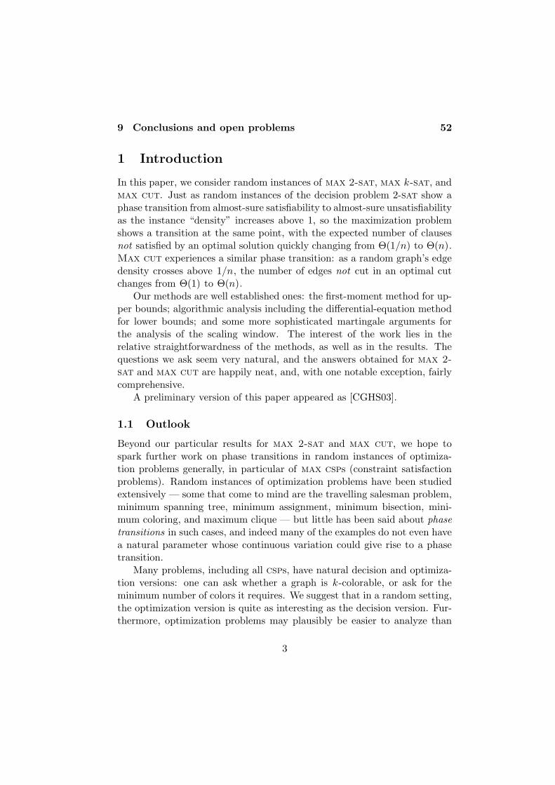
Figure 1: “Artist’s rendition” of the behavior of f(n, cn)/(cn).
this heuristic is doing as well as possible, it cannot yield an upper bound. Apromising alternative is to analyze the pure-literal rule, and we discuss thisin Section 5.2.5. For the meanwhile, though, we rely on [BBC+01] for theupper bound in Theorem 6 (with an extraneous logarithmic factor arisingin the translation), and we lack any upper bound for the λ > 1 case ofTheorem 7.
Figure 3 shows an “artist’s rendition” of the our results for 2-sat. Forc < 1, we expect to satisfy nearly all clauses, while for c → ∞, we expectto satisfy only about 3/4ths of them. The asymptotic behavior for c < 1is understood; so is that for c large (with a log-factor gap in the boundson the second term); and that for c = 1±Θ(n−1/3) (with only a one-sidedbound on the second term). We now state these results more exactly, andprove them in the next section.
For c < 1 a random formula F (n, cn) is satisfiable w.h.p., so we wouldexpect max F to be close to cn in this case; the following theorem showsthis to be true.
Theorem 4 For c = 1 − ε, with any constant ε > 0, bcnc − f(n, bcnc) =Θ(1/(ε3n)).
The proof comes from counting the expected number of the “bicycles”shown by [CR92] to be necessary components of an unsatisfiable formula.
For any c, f(n, cn) > 34cn, since a random assignment of the variables
satisfies each clause with probability 34 . The next theorem shows that neither
9

this bound nor the trivial upper bound cn is tight, although for large c, 34cn
is close to correct.
Theorem 5 For c large, (1 − oc(1))(√
c√
8−13√
π)n . f(n, cn) − 3
4cn .
(√
c√
3 ln(2)/8)n.
The values of√
8−13√
πand
√
3 ln(2)/8 are approximately 0.343859 and
0.509833, respectively. The upper bound is proved by a simple first-momentargument, and the lower bound by analyzing an algorithm; the upperbound’s proof technique is the same as that in [Spe94, Lecture 6] to an-alyze the Gale-Berlekamp switching game.
Our next results relate to the low-density case, when c is above but closeto the critical value 1. How does f(n, cn) depend on c = 1 + ε for small ε?
Theorem 6 For any fixed ε > 0, (1 + ε − [ε3/3 − 3ε4/8 ± O(ε5)])n .
f(n, (1 + ε)n); also, there exist absolute constants α0 and ε0 , such that forany fixed 0 < ε < ε0 , f(n, (1 + ε)n) . (1 + ε− 1
3α0ε3/ ln(1/ε))n.
That is, a constant fraction of the clauses must remain unsatisfied, butthis fraction — ε3/3 at most for ε sufficiently small — is surprisingly small.The lower bound is proved by using the “differential equation method” (seefor example [Wor95]) to exactly analyze a version of the unit-clause heuris-tic. The upper bound’s proof is a simple first-moment argument; however,for the probability that a sub-formula with density > 1 is satisfiable, itrequires the exponentially small bound given by Bollobas et al. [BBC+01](see Theorem 9 below). It is likely that, by replacing our use of [BBC+01]with structural properties of the kernel of a sparse random graph, the upperbound’s ε3/ ln(1/ε) could be replaced by ε3 to match the lower bound upto constants (see the Remarks in Section 5.2.5 and [J LR00, p. 123]).
The major significance of [BBC+01] was to determine the “scaling win-dow” for random 2-sat. Without using their result, we prove an analogousresult for max 2-sat, and incidentally reproduce most parts of their 2-satresult.
Theorem 7 Letting c = c(n) = 1 + ε(n) = 1 + λ(n)n−1/3 , for ε = o(1)(λ = o(n−1/3)) we have
bcnc − f(n, bcnc) =
O(λ3) if λ > 1;
Θ(1) if −1 6 λ 6 1;
Θ(|λ|−3) if λ < −1.
10

Furthermore, for λ > 1, for some positive absolute constant κ and anyβ > 0,
Pr(
(bcnc −max F (n, bcnc)) > κβ3λ3)
6 exp(−Ω(β)).
Also,
Pr(F (n, cn) is satisfiable) =
exp(−O(λ3)) if λ > 1;
Θ(1) if −1 6 λ < 1;
1−Θ(|λ|−3) if λ < −1.
In particular, in the scaling window c = 1 ± λn−1/3 , a random formulais satisfiable with probability which is bounded away from 0 and 1 (theexact bounds depending on λ), and it can be made satisfiable by removinga constant-order number of clauses (the constant depending on λ).
In section 6, for max k-sat, we derive analogous results only for c large,reflecting the general state of ignorance regarding the k-sat phase transi-tion. (For some results on scaling windows for k-sat see [Wil02].) Still moregenerally, Theorem 16 describes the high-density case for any max csp.More interestingly, for random max k-sat (including k = 2) we observethat max F is concentrated about its expectation f(n, cn) (as previously re-marked in [BFU93]) and that f(n, cn)/(cn) is monotone non-increasing in c.Were f(n, cn)/(cn) also monotone in n, an important property analogousto the satisfiability conjecture would follow; we present this as a conjecturefor general max csps.
In section 7 we consider online versions of max 2-sat, for one of whichwe prove that a natural greedy algorithm is optimal.
Results for the max cut problem for sparse random graphs, which isclosely analogous to random max 2-sat, are presented in section 8.
4 Random MAX 2-SAT
4.1 Sub-critical MAX 2-SAT
One of the most basic facts concerning max 2-sat is that for constantsc < 1, the expected number of clauses unsatisfied is o(1). This is refined byTheorem 4, which shows the number to be Θ(1/(ε3n)). We now prove thetheorem.
Theorem 4: Proof. We write the proof in the sat equivalent of the“G(n, p)” model, because the expressions for the probability of a clause’s
11

PSfrag replacements
u = w0
wi wj
v = wk+1
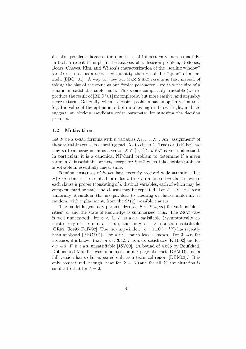
Figure 2: Sequence of clause-derived implications for a bicycle. Start thewalk from u, proceed clockwise to wi (which equals either u or u), continueright to wj , and again go clockwise to terminate at v (which equals eitherwj or wj ).
presence are cleaner in this model, but adaptation to the G(n, m) model isimmediate.
A k-bicycle (see Figure 4.1) is a sequence of clauses u, w1 , w1, w2 ,. . . , wk, v where literals w1, w2, . . . , wk are distinct as variables (none isthe same as nor the complement of another) and u ∈ wi, wi, v ∈ wj , wjfor some 1 6 i, j 6 k. (Think of it as a “walk” in which the first and lastvariables are also both visited en route.) Because satisfying a clause u, vmeans that if u is true then v must be true, such a clause yields an implica-tion u → v (and a complementary implication v → u); Figure 4.1 representssuch a sequence of implications for a bicycle. Chvatal and Reed [CR92] ar-gue that if a formula is infeasible then it contains a bicycle. Thus if wedelete an edge from every bicycle, the remaining subformula is satisfiable.
The number of potential k-bicycles, whether or not present in agiven formula F , is at most (2k)2(2n)k . The probability that all k + 1clauses of a given bicycle are present in a random formula F is at most[(cn)/(22
(
n2
)
)]k+1 = [c/(2(n− 1))]k+1 , so the expected number of k-bicyclesis . (2k)2ck+1/(2n). If we delete one edge in every bicycle, we obtain asatisfiable formula. For any fixed c = 1− ε < 1,
n∑
k=1
(2k)2ck+1/(2n) =2(2− ε)(1− ε)2
ε3n+ exp(−Ω(εn)).
Thus, the expected number of edges we need to delete is at most O(1/(ε3n))and f(n, bcnc) > bcnc −O(1/(ε3n)).
To obtain the lower bound we show that with probability at leastΘ(1/(ε3n)) the formula F is not satisfiable. This clearly implies an up-per bound f(n, bcnc) 6 bcnc − Θ(1/(ε3n)). To this goal we employ thesecond moment method.
For simplicity here, we will restrict ourselves to 3-bicycles, which will
12

only establish “Θε(1/n)”, that is, something of order Θ(1/n) but with hid-den constants that may depend on ε. The full proof is the same but usingbicycles of lengths up to 1/ε, not just length 3, and parallels the proof ofTheorem 7, case λ 6 −1. (In fact, taking λ = λ(n) = εn1/3 there establishesthe current theorem completely.)
Consider 4-tuples of clauses of the form u1, u2 , u2, u1 , u1, u3 , u3, u1,where u1, u2, u3 are arbitrary variables. One observes that this sequenceof clauses is a 3-bicycle, and, moreover, its presence in the random for-mula F implies non-satisfiability. We now show, using second momentmethod, that the number B3 of such bicycles is at least one with prob-ability at least Ω(1/n). We have E[B2
3 ] =∑
P(X ∈ F, X ′ ∈ F ), wherethe sum runs of over the pairs of 3-bicycles X, X ′ of the form above, andX ∈ F means all the clauses of X are present in F . We decompose thesum into three parts: the sum over pairs X, X ′ with X = X ′ , the sumover pairs that do not have common clauses and the rest. It is easy to seethat the first sum is simply E[B3] which is Θ(1/n), by the argument for up-per bound. To analyze the second sum note that for each fixed pair X, X ′
with no common clauses, we have P(X, X ′ ∈ F ) = P(X ∈ F )P(X ′ ∈ F ),when replacement of clauses is allowed. (When replacement is not allowedthe reader can check that the difference between the left and the right-hand sides is very small, and the rest of the argument goes through).Then, this sum is smaller than
∑
X,X′ P(X ∈ F )P(X ′ ∈ F ) = (E[B3])2 ,where the sum now runs over all the pairs X, X ′ . For the third sumwe have two cases. First case is pairs X, X ′ defined on the same setof variables. For example X = u1, u2 , u2, u1 , u1, u3 , u3, u1 andX ′ = u1, u2 , u2, u1 , u2, u3 , u3, u2, share one clause u1, u2 andare defined over the same set of variables. There are O(n3) choices for thevariables u1, u2, u3 in these pairs. But since X 6= X ′ then there are alto-gether at least five clauses in X and X ′ together. For a given pair, theprobability that all these clauses are present in F is O(1/n5). Then theexpected number of such pairs X, X ′ ∈ F is O(1/n2) = o(1/n).
The second case is pairs X, X ′ defined over different set of variables.Since they share a clause then the pair is defined on exactly four vari-ables. But then there are at least six clauses in this pair. We obtain thatthe expected number of such pairs X, X ′ which belong to F is at mostO(n4)O(1/n6) = O(1/n2) = o(1/n).
We conclude that E[B23 ] = E[B3] + o(1/n) = Θ(1/n) + o(1/n). We
now use the bound P(Z > 1) > (E[Z])2/E[Z2], which holds for any non-negative integer random variable Z . Applying this bound to B3 we obtainP(B3 > 1) > (E[B3])2/E[B2
3 ] > Θ(1/n2)/(Θ(1/n) + o(1/n)) = Θ(1/n). This
13

completes the proof.
It is worth pointing out the following simple fact, upon which we willshortly improve.
Remark 8 For c > 1, f(n, cn) & n( 34c + 1
4).
Proof. It suffices to show that for any ε > 0, for all n sufficiently large,f(n, cn) > (3
4c+ 14−ε)n. Select the first (1−ε)n clauses, and let ~X be a best
assignment for it. By Theorem 4, ~X satisfies an expected (1− ε)n− o(1) ofthese first clauses. Also, an expected 3/4ths of the remaining (c − 1 + ε)nclauses are satisfied, yielding the claim.
4.2 High-density random MAX 2-SAT
While it is well known that for c > 1, F (n, cn) is a.a.s. unsatisfiable, isit possible that even for c large, almost all clauses are satisfiable? Theo-rem 5 rules this out by showing that a constant fraction of clauses must gounsatisfied; up to a constant, it also provides a matching lower bound.
Theorem 5: Proof of the upper bound. The proof is by the first-momentmethod. A referee pointed out that “it seems odd to begin an estimate of thefirst moment with the first-moment method”, but that is exactly what wedo: We get at the expectation of max F through the probability that F hasa satisfiable subformula of some size, which (by the first-moment method)is at most the expected number of such subformulas. It is a little odd.
If max F > (1−r)cn then there is a satisfying assignment of a subformulaF ′ which omits rcn or fewer clauses, and where (taking F ′ to be maximal)all the omitted clauses are unsatisfied. Any fixed assignment satisfies each(random) clause of F ′ w.p. 3/4 and dissatisfies each omitted clause w.p. 1/4,so by linearity of expectations, the probability that there exists such an F ′
is
P = P(∃ satisfiable F ′) 6 2nrcn∑
k=0
(
cn
k
)
(3
4)cn−k(
1
4)k.
For r < 14 the last term is the largest and the sum is dominated by rcn
times the last term. From Stirling’s formula n! '√
2πn (n/e)n ,(
cn
rcn
)
' 1/√
2πr(1− r)cn · (r−r(1− r)−(1−r))cn.(3)
14

Substituting (3) into the previous expression,
P . 1/√
2πr(1− r)cn · 2n · rcn · (r−r(1− r)−(1−r)(3/4)1−r(1/4)r)cn.
Substituting r = 1/4− ε,
1
cnln P . ln(2)/c− (8/3)ε2 + O(ε3) + ln(rcn)/(cn),
so that for ε >√
(3/8) ln 2/c, as n →∞, P → 0. The conclusion follows.
Theorem 5: Proof of the lower bound. The proof is algorithmic. Whenvariables X1, . . . , Xt have been set, define the reduced formula Ft in whichany clause containing a True literal is removed and “scored”, and False lit-erals are removed from the remaining clauses. Define a potential functionq(Ft) to be the number of clauses already satisfied, plus 3/4 the number of2-variable clauses (“2-clauses”), plus 1/2 the number of 1-variable clauses(“unit clauses”). (Clauses with 0 variables remaining are permanently un-satisfied.) At this point, set Xt+1 in whichever of the two ways gives anFt+1 with larger value q(Ft+1). (Ties may be broken arbitrarily.) We nowanalyze this algorithm.
We will work in a model F (n, m), with a set of (2n)2 ordered clauses,allowing improper ones involving the same variable twice, and (as before)taking precisely m clauses uniformly at random with replacement from thisset. The expected number of improper clauses in F (n, c) is only Θ(c), andour conclusions for F (n, cn) carry over directly to F (n, m).
At any time t, randomly assigning the remaining variables satisfies (forany formula) an expected total number of clauses precisely q(Ft), so someassignment must achieve at least this. I.e., q(Ft) is a lower bound on thenumber of clauses satisfiable, q(F0) = 3
4cn, and we will focus on the incre-ments Ft+1 − Ft .
In Ft , let the number of appearances of Xt and Xt in unit clauses bedenoted by A1 and A1 , and their number of appearances in 2-clauses by A2
and A2 . If Xt+1 is set to True, then
q(Ft+1)− q(Ft) = ∆t.=
1
2(A1 − A1) +
1
4(A2 − A2),
and if Xk is set False, then q(Ft+1)− q(Ft) = −∆t . Thus q(Ft+1)− q(Ft) =|∆t|.
For most of the analysis we will only consider values of t between δn and(1− δ)n, where δ > 0 is any small value of our choosing. (We will take δ to
15

0 at the end of the proof.) Having chosen δ, we will consider only c > c0(δ),for some function c0 implicitly specified by the proof.
In the F model, the number of clauses m2(xn) containing none ofthe first xn variables is distributed as B(cn, (1 − x)2), with expectationµ2 = cn(1 − x)2 . For δ 6 x 6 1 − δ, by the Azuma-Hoeffding inequality,Pr(|B(cn, (1 − x)2) − µ2| > λ) 6 2 exp(−2λ2/(cn)). Setting λ = n−1/3µ2 ,Pr(|m2−µ2| > n−1/3µ2)) 6 2 exp(−2n1/3cδ4). Summing over the < n stepsunder consideration, the probability that m2 ever fails to be within 1±n−1/3
times its expectation is exponentially small, and we may simply ignore thesecases.
The same will be true of m1 , the number of unit clauses, but the argu-ment has additional complications. Denote by M ′
1 the set of clauses con-taining exactly one of the first xn variables: these include the m1 unitclauses and also already-satisfied clauses. m′
1 = |M ′1| is distributed as
B(cn, 2x(1 − x)), with expectation µ′1 = 2cnx(1 − x), and depends onlyon the random formula, not the algorithm. By the same argument as form2 , we may safely assume that for all δ 6 x 6 1− δ, m′
1(xn) is within therange (1± n−1/3)µ′1 .
Let L′1 ∈ [2xn]m′1 be the identities (“labels”) of the set literals in the
clauses M ′1 . The True or False settings ~X of the xn variables, together with
L′1 , determine which of the m′1 clauses are satisfied clauses, and which are
unit clauses contributing to m1 ; let us write m1 = m1(L′1, ~X). It is hard tocharacterize the setting ~X produced by the algorithm, and with it the “true”value of m1 , but for any ~X , m1(L′1, ~X) 6 m1(L′1)
.=∑xn
τ=1 maxsτ , sτ,where sτ and sτ are the numbers of occurrences in L′1 of Xτ and Xτ .
Let us first consider the expectation of Em1 over random L′1 , which is xntimes E maxs1, s1. Now s1 and s1 are respectively the number of headsand tails in a number of coin tosses itself distributed as B(m′
1, 1/(xn)),so this is no longer a question about an algorithm or random process butsimply a pair of random variables. We may assume that m′
1 = 2cnx(1 −x)(1 + on(1)), and in this case the Chernoff bound (1) shows that Pr(s1 −m′
1/(2xn) > k√
c) 6 exp(−k2c/[(2c(1 − x) + 23k√
c)]) 6 exp(−k/4), fork, c > 1. The probability that either s1 or s1 is “large” is at most twicethis, proving E maxs1, s1 = m′
1/(2xn) + O(√
c). We conclude that thereis a universal k0 such that for c sufficiently large,
1
2m′
1 6 Em1 61
2m′
1 + k0
√cxn.(4)
The Azuma-Hoeffding inequality (Theorem 3) shows that for randomlabelings L′1 , m1(L′1) is tightly concentrated around the mean given by
16

(4). Two labelings differing in a single label give values of m1 differingby at most 2, so even if m′
1 were fully cn, Pr(|m1 − Em1| >√
cn) 6
2 exp(−2cn2/(4cn)). Even when multiplied by the < n steps the algorithmruns, there is only a negligible, exponentially small probability of encounter-ing such a labeling (which is determined by the initial random formula andthe number of variables xn that have been set, independent of how they areset).
Similar, slightly easier arguments apply to m1 , and m1 6 m1 6 m1 , sowe may assume that for all δ 6 x 6 1−δ, |m1(xn)−cnx(1−x)(1+on(1))| 66√
c and (as before) that |m2(xn)− cn(1− x)2| 6 n−1/3cn(1− x)2 .Conditioned on any “history” giving values m1(xn) and m2(xn) in the
presumed ranges, for t = xn,
E|∆t| .= E|1
2(A1 − A1) +
1
4(A2 − A2)|,
where A1 and A1 are each distributed as B(m1, 1/(2(1−x)n)), and A2 andA2 as B(2m2, 1/(2(1 − x)n)). Again, this is no longer a question aboutan algorithm or random process but simply about four random variables.While the values within each pair are not independent, for large n (anduniformly over all δ 6 x 6 1 − δ), the constituents of ∆t converge toindependent Poissons or Gaussians. Specifically, (A1 − EA1)/
√c converges
in distribution to N(0, 12x) and (A2 − EA2)/
√c to N(0, 1 − x), the same
is true for A1 and A2 , and the joint distribution of the four “rescaled”variables converges to that of four independent Gaussians. The expectationof the given linear function of the original variables thus converges to (arescaling back of) the same function of the Gaussians, whose distribution is
a single Gaussian Z whose variance is σ2Z = 2 · 1
2
2 · x + 2 · 14
2 · (1 − x). It
is well known that E|N(0, σ2)| =√
2/πσ, and ∆t has mean exactly 0 (bysymmetry), so E|∆t| =
√cE|(∆t−E∆t)/
√c| =
√c(1 + oc(1) + on(1))E|Z| =
(1 + oc(1) + on(1)) ·√
2/π√
c√
12x + 2(1− x).
We conclude that the expected number of clauses satisfiable is at least
q(Fn) > q(F0) +
(1−δ)n∑
t=δn
E|∆t|
>3
4cn + (1 + oc(1) + on(1))
√
2/π√
c n
∫ 1−δ
δ
√
1
2x + 2(1− x) dx
=3
4cn +
√8− 1
3√
π
√c n · (1 + oc(1) + oδ(1) + on(1)).
17

Taking δ → 0 and c →∞ together appropriately yields the claim: the oδ(1)is subsumed into the oc(1), we write −oc(1) to highlight the pessimisticpossibility, and the on(1) is expressed by the Theorem’s “.” notation.
We remark that in the preceding proof, Xk was set True or False so as tomaximize half the number of satisfied unit clauses plus a quarter the numberof satisfied 2-clauses. This is reminiscent of the “policies” in [AS00]. There,the goal was to satisfy as a dense a 3-sat formula as possible; unit clausesalways had to be satisfied, and variables were set so as to maximize a linearcombination of the number of satisfied 2-clauses and 3-clauses. In [AS00],the linear combination which was optimal for the purpose changed during thecourse of the algorithm; the determination of the optimal combinations, andthe proof of optimality, was a main result of the paper. In the present case,though, it is evident that the ratio 1:2 is optimal: for c large, the potentialfunction q predicts the expected number of clauses satisfiable almost exactly.The difference can be ascribed to the fact that here c is “large”, and in [AS00]the corresponding parameter (the initial 3-clause density) was fixed (relevantvalues were in the range of 3.145 to 3.26). Were we to try to tune the max
2-sat algorithm above for small values of c, more complex methods likethose of [AS00] would presumably be needed.
4.3 Low-density random MAX 2-SAT
For low-density formulas, with c = 1 + ε and ε > 0 a small constant, thebounds of Theorem 5 are inapplicable. It is still true (from Remark 8) thatwe expect to satisfy at least (1 + 3
4ε)n clauses, but it is not obvious whetherthe best answer is this, or close to the full number of clauses (1 + ε)n, orsomething in between. In this section we prove Theorem 6 which shows that(1 + ε)n − f(n, cn), the number of clauses we must dissatisfy, lies betweenΘ(ε3n/ ln(1/ε)) and Θ(ε3n). That is, a linear fraction of clauses must berejected, but this fraction, at most Θ(ε3), is surprisingly small. We willemploy the following theorem of Bollobas et al. [BBC+01] on random 2-sat.
Theorem 9 ([BBC+01], Corollary 1.5) There exist positive constants α0
and ε0 such that for any 0 < ε < ε0 and sufficiently large n, P[F (n, (1 +ε)n) is satisfiable] 6 exp(−α0ε
3n).
(Here, α0 is the lim inf of the constant implicit in Θ in the theoremin [BBC+01].) The exp(−Θ(ε3n)) probability of satisfiability in random2-sat translates into an expected O(ε3n/ ln(1/ε)) unsatisfied clauses in ran-dom max 2-sat.
18

Theorem 6: Proof of the upper bound. The proof is by the first-momentmethod. Let c = 1 + ε. Let F ′ range over subformulas of F which omit rcnor fewer clauses. Specifying r < 1/4, the conditions of Theorem 9 apply, so
P = P(∃ maximally satisfiable F ′) 6
rcn∑
k=0
(
cn
k
)
(1
4)ke−α0(ε− k
n)3n;(5)
as r < 1/4, the sum is dominated by the last term. Using (3) to approximate(
cncrn
)
,
1
cnln P . −r ln r − (1− r) ln (1− r)− α0(ε− cr)3/c− r ln(4).
First observe that as ε → 0, for any r = o(ε), this is
= −r ln r(1 + o(1))− α0ε3(1 + o(1))− r ln(4).
For any constant b < 1/3, if r = bα0ε3/ ln(1/ε), this is
= 3bα0ε3(1 + o(1))− α0ε
3(1 + o(1)) < 0.
That is, it is unlikely that asymptotically fewer than (1/3)α0ε3/ ln(1/ε)
clauses can go unsatisfied.
Theorem 6: Proof of the lower bound. The proof is algorithmic, and of thesort familiar from [AS00] and similar works. It analyzes a variation on the“unit-clause” heuristic through the differential equation method. Initially,“seed” the algorithm by artificially adding some number δn of unit clauses,where δ = δ(ε) will be very small. While F has any unit clauses, select oneat random and set its variable to satisfy the clause. Continue until no unitclauses remain. The analysis consists of counting the clauses unsatisfied inthese steps, and justifying the assertion that when there are no more unitclauses, o(1) further clauses need be unsatisfied.
When t variables have been set, let the number of 2-clauses be denotedm2(t), and the number of unit clauses m1(t). In one step, assuming thatm1 > 0 before the step, the expected changes in these quantities are
E(∆m2) = − 2m2
n− t= −2m2
n
1
1− t/n,(6)
E(∆m1) = −1− m1
n
1
1− t/n+
m2
n
1
1− t/n.(7)
19

These (small) random changes are predictable in the long run: the analysisis a fairly standard application of the differential equation method. We usethe “packaging” of the method given by Wormald’s [Wor95, Theorem 2].Theorem 2 is too long to re-state explicitly, but we will summarize thehypotheses and conclusion as we show how they apply to our process.
The first hypothesis is that, over the entire space, ∆m1 and ∆m2 have“light tails”. For Wormald’s Theorem 2, choosing “w”= n0.6 and “λ”= n0.1 ,it suffices to show that, conditioned on any “history” of the process upto time t, for i = 1, 2, Pr(|∆mi| > n0.2) = o(n−3). The changes ∆mi
are bounded by the number of appearances of the variable Xt , which isdominated by a binomial random variable B(2cn, 1/(n− t)). For t 6 n/2,the Chernoff bound (1) gives Pr 6 exp(−n0.2), which is better than needed.We treat t > n/2 (which will not be of genuine interest) by replacing thealgorithmic random process with an artificial one in which the changes ∆mi
are deterministically those given by the right-hand sides of (6) and (7).While we are at it, we will also artificially apply (7) even for m1 6 0; it willbe seen that during the period to which we apply the differential-equationanalysis, this condition will never be relevant.
The second condition needed by Wormald’s theorem is that the expectedchanges in ∆mi must be expressible as Emi = fi(t/n, m1/n, m2/n) + o(1).Equations (6) and (7) do so.
The third and final condition needed is that the functions fi(s, z1, z2)should be Lipschitz continuous in some open connected domain D withprescribed properties. The subspace D with |s| < 1/2, |zi| < 2c will do,and it is clear that the functions are Lipschitz here.
The first conclusion is that for a given initial condition (0, z1, z2), thedifferential equations dzi/ds = fi(s, z1, z2) have a unique solution z(s). Inour case, starting with z2(0) = c and z1(0) = δ the solution is simply
z2(s) = c(1− s)2
z1(s) = cs(1− s) + (1− s) ln(1− s) + δ(1− s).(8)
The second conclusion is that, starting from mi/n = zi , the random processalmost surely satisfies mi(t) = nzi(t/n) + o(n).
Equation (8) gives z1 = 0 only when s = s? satisfies
c =− ln(1− s?)− δ
s?.(9)
Although both s? and δ are functions of c, it is more convenient toparametrize c and δ as functions of s? . At this point, we will define δ = s?5 .
20

Equation (9) is important because it justifies the assumption m1 > 0 (madebefore equation (6)) for all fixed s < s? . Once m1 = 0 (which a.a.s. willoccur at some time s ∈ [s?−δ, s?+d]) we will halt the algorithm and analyzethe remaining formula by other means. To first order, (9) gives c = 1 + εwhen s? = 2ε, and thus for ε sufficiently small, our earlier limitation tot 6 n/2 is also justified.
While s < s? , the only clauses ever unsatisfied are unit clauses whichcontain the negation of the variable being set, and the expected number ofsuch rejected clauses per step is m1/(2(n− t)) = z1/(2(1− s)). Integratingover the period 0 to s? ,
∫ s?
0
z1
2(1− s)ds =
1
2
∫ s?
0(cs + ln(1− s) + δ) ds
=1
2
(
cs2/2− (1− s) ln(1− s)− s + δs)
∣
∣
∣
∣
s?
0
which, substituting for c from (9)
= −1
4(2− s?) ln(1− s?)− 1
2s? +
1
4δs?.(10)
From s = 0 to s = s? , the number of clauses dissatisfied by the algo-rithm is a.a.s. a.e. n times expression (10). At time s = s? , the remaining(uniformly random) 2-sat formula has density z2 / (1 − s?) = c(1 − s?) =− ln(1−s?)−δ
s? (1− s?); with δ = s?5 , this is 1− s?/2−O(s?2), which is < 1 fors? sufficiently small. Thus by Theorem 8 the remaining formula contributeso(1) to the expected number of unsatisfied clauses.
In short, the number of clauses not satisfied is a.a.s. a.e. n times ex-pression (10). For s? asymptotically close to 0 and with δ = s?5 , this isn(s?3/24 + s?4/24 +O(s?4)), while from (9), c = 1 + s?/2 +O(s?2). Return-ing to the original parametrization, with ε > 0 asymptotically small andc = 1 + ε, s? = 2ε − 8ε2/3 ± O(ε3), and the number of dissatisfied clausesis a.a.s. n(ε3/3− 2ε4/3±O(ε4))(1 + on(1)).
Three remarks. First, the δn artificial unit clauses are introduced solelyto exclude the possibility that m1 = 0 at some early time, long before thetime of about 2ε (for c = 1+ε) when the work is really done. This simplifiesthe proof but is not necessary: if we use the shortest-clause rule, there maybe a few early revisits to m1 = 0, but then m1 will “take off” and notreturn to 0 until time about 2ε. Our proof for the “scaling window” resultof Theorem 7 uses this approach. So let us now imagine δ = 0.
21
In that case, our second remark is that in addition to the asymptote,the proof gives a precise parametric relationship (as functions of s?) be-tween the clause density c (given by (9)) and the rejected-clause density(given by (10)). For example, for c = 1.5 we find rejected-clause density≈ 0.0183275, and for c = 2 — where naively the rejected-clause densitywould be 1
4c = 0.5 — we achieve rejected-clause density ≈ 0.0809517.Third, with the solution in hand, the asymptotic behavior is easy to
see without the need for differential equations. This approach is not herepresented formally, but it is more intuitive and more robust, and is the basisfor the analysis within the scaling window (see Theorem 7).
Theorem 6: Informal argument for the lower bound. Consider what hap-pens when m = (1 − δ)n variables remain unset. The number of 2-clausesis a.a.s. m2 ' (1− δ)2(1 + ε)n ' (1 + ε− 2δ)n. The expected increase in thenumber of unit clauses is then E(∆m1) = −1−m1/m+m2/m > −1+m2/m(and the neglected m1/m is not only conservative, but will also prove to beinsignificantly small). Thus, E(∆m1) > −1+[(1+ε−2δ)n]/[(1−δ)n] ' ε−δ.At δ = 0, the number of unit clauses increases by ε per step, this increaselinearly falls to 0 per step by δ = ε, and further to −ε by δ = 2ε: theexpected number of unit clauses is bounded by an inverted parabola, withbase 2εn and height 1
2ε2n. At each step about 1/(2n)th of the unit clausesget dissatisfied. The area under the parabola, times this 1/(2n) factor, is23 · base · height · 1/(2n) = 1
3ε3n.
5 The MAX 2-SAT scaling window
For random max 2-sat, we have seen that for fixed c < 1, bcnc −f(n, bcnc) = Θ(1/n), and for c > 1, cn− f(n, cn) = Θ(n). That is, randommax 2-sat experiences a phase transition around c = 1. It is natural to askabout the scaling window around the critical threshold: What is the intervalaround c = 1 within which bcnc − f(n, bcnc) = Θ(1)? Theorem 7 showsthat the scaling window is c = 1 ± Θ(n−1/3). The corresponding questionfor random 2-sat is the range in which P(F (n, bcnc) is satisfiable) = Θ(1).This was shown by [BBC+01] to be c = 1 ± Θ(n−1/3) with their resultreproduced as Theorem 10 here.
Theorem 10 (Bollobas et al, [BBC+01]) Let F (n, cn) be a random 2-sat formula, with c = 1+λnn−1/3 . There are absolute constants 0 < ε0 < 1,0 < λ0 < ∞, such that the probability F is satisfiable is: 1 − Θ(1/|λn|3),when −ε0n
1/3 6 λn 6 −λ0 ; Θ(1), when −λ0 6 λn 6 λ0 ; and e−Θ(λ3n), when
22
λ0 6 λn 6 ε0n1/3 .
That the two scaling windows are the same is no coincidence, and in factTheorem 7 reestablishes much of Theorem 10 independently. Unfortunately,our theorem does not capture everything one would like to know about thescaling window.
Theorem 7: Proof. Note that, provided we prove the bounds for the casesλ 6 −1 and λ > 1, the bound for the case |λ| < 1 follows immediately, sincewe obtain that the probability of satisfiability is at least exp(−O(λ3)) >
exp(−O(1)) and at most 1 − Θ(1/|λ|3) 6 1 − Θ(1), where in both cases|λ| < 1 was used. The more interesting cases |λ| > 1 are considered in thetwo subsections below.
5.1 Case c = 1 + λn−1/3, λ 6 −1
For convenience we write c = 1 − λn−1/3 and λ > 1. The proof for thiscase is very similar to that of Theorem 4 and uses the notion of bicycles.(As in the earlier case, we work in the equivalent of the G(n, p) model fornotational convenience, with the understanding that the proof works equallywell in the G(n, m) model.) As before, the number of clauses that must bedissatisfied is bounded by the number of bicycles. The expected number ofk-bicycles is at most (2k)2ck+1/(2n) = (2k)2(1 − λn−1/3)k+1/(2n). Using
the formula∑
k>1 k2ρk = ρ(1+ρ)(1−ρ)3
which for ρ ' 1 is ' 2/(1− ρ)3 , we have
∑
16k<∞(2k)2(1− λn−1/3)k+1/(2n) ' 4/λ3.(11)
Therefore bcnc − f(n, bcnc) = O(1/λ3). By the first-moment method, theprobability that the formula is unsatisfiable is at most the expected numberof bicycles, that is, at most O(1/λ3).
We now obtain a matching lower bound. Consider only “bad” bicycles,in which u = wi , v = wj , and i < j . Note that no bad bicycle is completelysatisfiable, since the first “wheel” u → · · · → wi = u requires u = Falseand thus wi = True; whereupon the path (technically called the “top tube”of a bicycle) wi → · · · → wj implies wj = True; and the second wheelwj → · · · → v = wj provides a contradiction. Note that about 1/8th of thepotential bicycles are bad.
23

Let Bk denote the number of bad k-bicycles. Since
E(#unsatisfiable clauses) > Pr(F unsatisfiable)(12)
> Pr(∑
k6K
Bk > 1),
it suffices to prove that this is
= Ω(1/λ3);(13)
we will show this for K = (1/λ)n1/3 . Repeating the argument for (11), weobtain that
E[∑
k6K
Bk] & (2/(8e))/λ3,
the 1/(8e) coming from the series’ truncation at K and the use of only badbicycles. To obtain (13) it suffices to prove that
E[(∑
k6K
Bk)2] = (1 + O(1)) · E[∑
k6K
Bk],(14)
for then
P(∑
k
Bk > 1) >(E[∑
k Bk])2
E[(∑
k Bk)2]=
(E[∑
k Bk])2
E[∑
k Bk](1 + O(1))= Ω(1/λ3).
We will prove (14) with O(1/λ3) filling in for O(1) (recall that λ > 1).Consider pairs of k, k′-bicycles X, X ′ with k, k′ 6 K . It suffices to showthat for every X ,
∑
X′ 6=X
P(X ′ ⊆ F |X ⊆ F ) = O(1/λ3),(15)
because then
E[(∑
k
Bk)2] =∑
X,X′
P(X, X ′ ⊆ F )
=∑
X
Pr(X ⊆ F ) [1 +∑
X′ 6=X
Pr(X ′ ⊆ F | X ⊆ F )]
6 E[∑
k
Bk](1 + O(1/λ3)).
24

Establishing (15) is the nub of the proof. First, observe that for anybicycle X ′ sharing no literals with X , Pr(X ′ ⊆ F | X ⊆ F ) 6 Pr(X ′ ⊆ F ),and so such bicycles X ′ contribute 6 E
∑
k Bk = O(1/λ3) to the sum.Given a bicycle X ′ = u, w1 , w1, w2 , . . . , wk, v, a sequence of lit-
erals wi, wi+1, . . . , wj from X ′ is defined to be a type I excursion if literalswi, wj belong to X but literals wi+1, . . . , wj−1 do not (i.e., the sequencebranches off from X and rejoins it). (If j = i + 1, a sequence wi, wi+1 is atype I excursion if the corresponding clause (wi, wi+1) ∈ X ′ does not belongto X .) A sequence of literals u, w1, . . . , wj in X ′ is defined to be a type IIexcursion if the literal wj belongs to X , but u, w1, . . . , wj−1 do not (i.e., a“prefix” of X ′ merges into X ). Similarly, a sequence wj , wj+1, . . . , v in X ′
is defined to be a type III excursion (i.e., a suffix of X ′ branches off fromX ).
Bicycles X ′ which are neither equal to X nor disjoint from X musthave at least one excursion (and at most one each of excursions of type IIand III). It suffices to establish (15) for such bicycles X ′ . We will just showthat the expected number of bicycles X ′ with one type II excursion, notype III excursion, and any number r > 0 of type I excursions, is O(1/λ3);the other three cases (classified by the number of type II and III excursions)follow similarly.
Since a collection of excursions uniquely defines X ′ , it is enough tocount such collections. Let the lengths of the type I excursions bem1, m2, . . . , mr > 2 and that of the type II excursion mII , where the lengthis defined by the number of literals.
For each type I excursion there are two endpoints (literals) which be-long to X . Since the size of X is 6 K = (1/λ)n1/3 , there are 6 K2r =(1/λ2r)n2r/3 choices for all the end points. The ith type I excursion con-tains mi − 2 literals not from X , so there are at most (2n)mi−2 ways ofselecting them. The excursion contains mi − 1 clauses, all not from X , sothe probability they are all present in F is (1− λn−1/3)mi−1/(2n)mi−1 .
Similarly, for the type II excursion, there are at most K choices for theendpoint literal wj , which belongs to X , at most K choices for the initialliteral u (which must be the negation of another literal chosen for X ′), andat most (2n)mII−2 choices for other literals u, w1, . . . , wj−1 . The excursioncontains mII − 1 clauses, all not from X , so the probability that they areall present in F is (1− λn−1/3)mII−1/(2n)mII−1 .
Combining, we obtain that the expected number of bicycles X ′ con-taining exactly r type I excursions, one type II excursion, and no type III
25
excursions is
#(r, 0, 1) 6∑
mII ,m1,...,mr>2
(1/λ2r+2)n2r+ 2
3 (2n)mII−2+∑
imi−2r
× (1− λn−1/3)mII−1+∑
imi−r
(2n)mII−1+∑
imi−r
=1
2r+1λ2r+2nr+ 1
3
∑
mII ,m1,...,mr>2
(1− λn−1/3)mII−1+∑
imi−r.
Note that∑
mII ,m1,...,mr>2
(1− λn−1/3)mII+∑
imi−r−1
=∑
mII ,m1,...,mr>1
(1− λn−1/3)mII+∑
imi
=
∑
m>1
(1− λn−1/3)m
r+1
61
λr+1n−r+ 1
3
.
Applying this to the equality above we obtain
#(r, 0, 1) 61
2r+1λ3r+3, and
∑
r>0
#(r, 0, 1) 61
2λ3 − 1= O(1/λ3).
With similar calculations for #(r, ·, ·) this establishes (15), and completesthe proof of the case λ 6 −1 of Theorem 7.
5.2 Case c = 1 + λn−1/3, λ > 1
The proof of this part resembles our alternate, informal argument for thelower bound of Theorem 6. There we showed that m1(t) a.a.s. a.e. followeda parabolic trajectory. Both there and here, at time t = εn, the expectationgiven by the parabola is 1
2ε2n, and the typical deviations (the standard devi-ation) from summing εn binomial r.v.s with distributions near to B(n, 1/n)is about
√εn.
In the previous case, with ε = Θ(1), the deviations were a.a.s. tinycompared with the expectation, but here, with ε = λn−1/3 , if λ = Θ(1)
26

unit
clause
s
algorithm steps 2εn
12ε2n
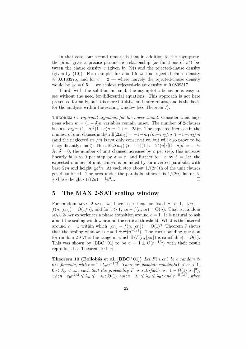
Figure 3: Nominal parabolic trajectory of m1(t) vs t, and two randomsamples for density 1 + λn−1/3 (λ = 2, n = 10, 000). With λ = Θ(1), therandom fluctuations are of the same order as the nominal values.
the standard deviation√
λn1/3 is of the same order (in terms of n) as theexpectation 1
2λ2n1/3 : the trajectory is not predictable in an a.a.s. a.e. sense.Figure 3 shows two typical samples (with λ = 2 and n = 10, 000) againstthe nominal parabolic trajectory. The analysis is thus more involved.
As before, we analyze the unit-clause resolution algorithm in which ifthere are any unit clauses (if m1(t) > 0) we choose one at random and setits literal True, and otherwise we choose a random literal (from the variablesnot already set) and set it True.
Our analysis proceeds in three phases. Phase I proceeds until time T =2εn, and we show that in this period, there is an exponentially small chancethat m1 is ever much larger than its expectation. In Phase II, we continueunit-clause resolution until m1(t) = 0; we show that this happens quickly,and the number of unit clauses is unlikely ever to grow much beyond itsinitial Phase II value. These facts will suffice to give upper bounds on thesum, over all steps in these phases, of the number of unit clauses at eachstep, and in turn on the number of unsatisfied clauses. In Phase III we beginwith a formula of density 6 1−εn, and we simply apply the Theorem’s caseλ 6 −1, proved (non-algorithmically) in Section 5.1.
27

5.2.1 Useful facts
We first establish a simple relation, useful for Phase I and essential forPhase II. The number of 2-clauses remaining (both of whose variables re-main) at time δn is m2(δn) ∼ B(n(1 + ε), (1 − δ)2). Thus for all timest 6 1
2n(1 + ε) (much longer than the times Θ(εn) in which we are inter-ested),
Pr
(
maxδ6 1
2
[
m2(δn)− n(1 + ε)(1− δ)2 > n3/5]
)
6 exp(−Θ(n1/5)).(16)
We prove (16) using the Chernoff bound (1). To establish (16) we take(1 + ε)n i.i.d. Bernoullis with pi = (1 − δ)2 . For any fixed δ in (16) thisimmediately gives probability exp(−Θ(n6/5/n)), and the sum over the Θ(n)possible values of δ can be subsumed into the exponential.
In the main we will therefore assume that
m2(δn) 6 n(1 + ε)(1− δ)2 + n3/5,(17)
and deal with the failure case only at the end.We will also need two simple distributional inequalities. First, a
Bernoulli random variable is stochastically dominated by a similar Poissonrandom variable,
Be(p) Po(− ln(1− p)),
as they give equal probability to 0, and the Bernoulli’s remaining probabil-ity is entirely on 1 whereas the Poisson’s is on 1 and larger values. (Herewe have written Be(p) and Po(− ln(1 − p)) where we really mean randomvariables with those distributions; we shall continue this practice where con-venient.) Summing n independent copies of such random variables showsthat a binomial is dominated by a similar Poisson,
B(n, p) Po(−n ln(1− p)).
In particular, for any a, b = Θ(1),
B(an, b/n) Po(−an ln(1− b/n)) = Po(ab + O(1/n))).(18)
We also recall that the exponential moments of a Poisson random vari-able are
EzPo(d) = exp((z − 1)d).(19)
We now analyze the unit-clause algorithm in Phases I and II.
28

5.2.2 Phase I
During Phase I, assuming (17), at times t = δn,
m2(t) = n(1 + ε)(1− δ)2 + O(n3/5) 6 n(1 + 1.01ε− 2δ),
using ε > n−1/3 . Meanwhile the number of unset variables is m(t) = n(1−δ), so in particular,
m2(t)/m(t) 6 1 + 1.05ε.(20)
With the random variables below all independent, the unit-clause algo-rithm gives
m1(t)−m1(t− 1)
= −1 + 1(m1(t− 1) = 0)−B(m1(t− 1), 1/(m(t− 1)))
= +B(m2(t− 1), 1/(m(t− 1)))
6 −1 + 1(m1(t− 1) = 0) + B(m2(t− 1), 1/(m(t− 1)))
6 −1 + 1(m1(t− 1) = 0) + Po(1 + 1.1ε),
where the last inequality uses (18), (20), and 0.1ε 1/n.It is easy to see that, starting from m1(0) = m′
1(0), if X(t) 6
Y (t) for all t , if
m1(t)−m1(t− 1) = 1(m1(t− 1) = 0) + X(t− 1) and
m′1(t)−m′
1(t− 1) = 1(m′1(t− 1) = 0) + Y (t− 1),
then for all t,
m1(t) 6 m′1(t).
(An easy proof is inductive. The 1(·) term may contribute to m1 and notto m′
1 if m1 < m′1 , but in that case, the inequality still holds.) In a similar
setup but with X(t) Y (t), coupling shows that m1(t) m′1(t).
Thus m1(t) m′1(t) where m′
1(0) = 0 and
m′1(t)−m′
1(t− 1) = −1 + 1(m′1(t− 1) = 0) + Po(1 + 1.1ε).
Now, let U(t) be a random walk with U(0) = 0 and independent increments
U(t)− U(t− 1) = −1 + Po(1 + 1.1ε),(21)
29

and let V (t) count the “record minima” of U , so V (0) = 0 and V (t) =V (t − 1) except that if U(t) < minτ<t U(τ), then V (t) = V (t − 1) + 1.Observe that
m1(t) m′1(t) = U(t) + V (t).(22)
(V (t) precisely takes care of the 1(·) terms.)At this point, we have reduced the behavior of the number of unit clauses
m1(t) to properties of a simple Poisson-incremented random walk.
Renewal process V
We first dispense with V , by showing that
V (∞).= sup
t>0V (t) G(2ε),(23)
where G(p) indicates a geometric random variable with parameter p. Start-ing from any time t0 at which U(t0) is a record minimum (at whichV (t0) = V (t0 − 1) + 1), define U ′(τ) = U(t0 + τ) − U(t0) + 1. Observethat U ′(0) = 1, and the first time τ for which U(τ) = 0 gives the next timet0 +τ for which V (t0 +τ) = 1. Thus the number of “restarts” of the processU ′ is V (∞).
U ′ may be viewed as a Galton-Watson branching process observed eachtime an individual gives birth (adding Po(·) offspring to the population)and itself dies (adding −1). As a super-critical Galton-Watson branchingprocess, U ′ has a positive probability of non-extinction, and thus the numberof restarts (following extinctions) is geometrically distributed.
Quantitatively, the extinction probability of a Galton-Watson processwith X offspring (the probability the process never hits 0) is well known tobe the unique root p ∈ [0, 1) of
p = E(pX).(24)
(See for example [Dur96, pp. 247–248].) Also, for any p such that p > E(pX),the probability of non-extinction exceeds 1 − p. In this case, recalling (21)and (19), we seek p such that
p > E(pX) = exp((p− 1)(1 + 1.1ε))
or equivalently, with q = 1− p,
ln(1− q) > −q(1 + 1.1ε).
30

Taking a Taylor expansion around q = 0 and cancelling like terms, it sufficesto ensure that 1
2q + 13q2 + · · · < 1.1ε, and q = 2ε suffices (for all ε < 0.37,
let alone the ε = Θ(n−1/3) of interest).Thus U ′ has non-extinction probability at least 2ε, verifying (23).
Random walk U
We now analyze the random walk U (see (21)) to show that for any 0 <ε 6 0.02 and 0 < α 6 0.06 (our principal realm of interest will be ε, α =Θ(n−1/3)), for any time t,
Pr
(
max06τ6t
U(τ) > EU(t) + αt
)
6 exp(−tα2/2.1).(25)
Observe that U(t) is a submartingale, and for any β > 0 (by convexity ofexp(βu)), exp(βU(t)) is a non-negative submartingale.
Doob’s submartingale inequality (see for example [Nev75, p. 69]) assertsthat for a positive, integrable submartingale Xn , for all n ∈ N and alla ∈ R+ , a Pr(supm6n Xm > a) 6
∫
supm6n Xm>a XndP . Applying the
weaker form Pr(supm6n Xm > a) 6 EXn to 1a exp(βU(T )) gives
Pr
(
max06τ6t
U(τ) > EU(t) + αt
)
= Pr
(
max06τ6t
exp (βU(τ)) > exp (β(EU(t) + αt))
)
6E (exp(βU(t)))
exp (β(EU(t) + αt)).(26)
Trivially,
EU(t) = −t + (1 + 1.1ε)t = 1.1εt,(27)
and, by (19),
E (exp(βU(t))) = exp(−βt + β Po((1 + 1.1ε)t))
= exp(−βt) exp((eβ − 1)(1 + 1.1ε)t),
so (26) is
exp(−t[β − (1 + 1.1ε)(eβ − 1) + β(1.1ε + α)]).(28)
31

We are free to choose β > 0 as we like, so to minimize (28) we maximize theinnermost quantity. Setting its derivative equal to 0 yields 1−(1+1.1ε)eβ +1.1ε + α = 0 or β = ln(1 + α/(1 + 1.1ε)), but we will simply take β = α.Then (eschewing asymptotes in favor of absolute bounds), for ε < 0.02 andα < 0.06 (let alone the regime ε, α = Θ(n−1/3) of interest), (28) is
6 exp(
−tα2/2.1)
,
proving (25).
Parameter substitution and m1
Recall that ε = λn−1/3 with λ > 1, and parametrize time as t = βεn =βλn2/3 , restricting to β > 1. We will allow values t > n: U(t) is welldefined for all time, and (22) remains true if we define m1(t) = 0 for t > n.In (25), parametrize α by α = α′/
√t. Validity of (25) is then guaranteed
up to α′ = 0.06n1/3 , as α = α′/√
βλn2/3 6 0.06. With these substitutionsfor t and α in (25),
Pr( maxτ6βεn
U(τ) > βλ2n1/3 + α′√
βλn1/3) 6 exp(−α′2/2.1).
I.e., with β, λ > 1, the tails of U(t) fall off exponentially with a “half-life”,√βλn1/3 , smaller than the bound on the mean, βλ2n1/3 . A weaker but
more convenient form of the above inequality is
Pr( maxτ6βεn
U(τ) > 2α′βλ2n1/3) 6 exp(−Ω(α′2)).(29)
V (∞) has expectation 1/(2ε) = 12λn1/3 6 1
2βλ2n1/3 , which is smallerthan the bound on U ’s mean, and (as a geometric random variable) fallsoff exponentially with half-life comparable to its own expectation. Thusfrom (22), for 1 6 α′ 6 n1/4 6 0.06n1.3 ,
Pr
(
maxτ6βεn
m1(τ) > 3α′βλ2n1/3
)
= exp(−Ω(α′2)) and(30)
Pr
(
βεn∑
τ=1
m1(τ) > 3α′β2λ3n
)
= exp(−Ω(α′2)).(31)
In particular, with t = 2εn, or β = 2, (30) provides the following bound onthe number of unit clauses m1(t) at the end of Phase I.
Pr
(
maxτ62εn
m1(τ) > 6α′λ2n1/3
)
= exp(−Ω(α′2)).(32)
32
The probability of a deviation with α′ > n1/4 is exp(−Ω(n1/2)), and willbe dealt with as a “failure probability” at the end.
5.2.3 Phase II
The analysis of this phase largely parallels the previous one.Assuming (17), at times t = δn, m2(t)/m(t) is roughly (1 + ε)(1 − δ),
and in particular, since in Phase II by definition δ > 2ε,
m2(t)/m(t) 6 1− 0.95ε.(33)
Since Phase II ends as soon as m1(t) = 0, there is no +1(·) term toworry about, so assuming (33),
m1(t)−m1(t− 1)
= −1−B(m1(t− 1), 1/(2m(t− 1))) + B(m2(t− 1), 1/(m(t− 1)))
6 −1 + Po(1− 0.9ε).
By the same argument as for Phase I, then,
m1(2εn + t) m1(2εn) + W (t)
where W (t) is a random walk with W (0) = 0 and independent increments−1 + Po(1− 0.9ε).
We now fix α1 and condition on Phase I ending with m1(2εn) ≤α1λ
2n1/3 . Fix α2 > 2α1 . Our next goal is to bound the probability thatthe Phase II does not end by time 2εn + α2εn. Such an event occurs onlyif W (α2εn) > −m1(2εn) > −α1ε
2n > −12α2ε
2n. We have
Pr(W (α2εn) > −12α2ε
2n)
= Pr(
Po(α1εn(1− .9ε)) > E(Po(·)) + 0.4α2ε2n)
6 exp
(
− (0.4α2ε2n)2
α2εn(1− 0.9ε) + 0.4α2ε2n
)
since the Chernoff bound (1) applies as well to the Poisson. Substitutingε = λn−1/3 , and noting that the denominator’s first term, of order Θ(α2εn),dominates the second, of order Θ(α2ε
2n), we obtain
Pr(W (α2εn) > −12α2ε
2n) 6 exp(−0.42α2λ3).(34)
Then, conditionally on Phase I ending with m1(2εn) ≤ α1λ2n1/3
(see (30)), for any α2 > 2α1 , (34) implies that Phase II ends by time2εn + α2εn, with probability exponential in α2 .
33

Furthermore, over Phase II, m1(t) is unlikely ever to increase much overits initial value. An argument along the lines used in the context of equa-tion (24) could be constructed to show that maxt>0 W (t) is exponentiallysure to be quite small, but as there are some technical complications, wetake a simple, wasteful approach. Observe that
W (t) X(t)
where X(0) = W (0) = 0 and X(t) has independent increments −1+Po(1+1.1ε). This wild over-estimation is useful because X (unlike W ) is a sub-martingale, to which we apply Doob’s inequality. In fact X is the samerandom process as U , so the tail inequality of (29) applies to X in lieuof U . We obtain that for every α2, α
′ > 1
Pr( maxτ6α2εn
X(τ) > 2α2α′λ2n1/3) 6 exp(−Ω(α′2)).(35)
We finish the analysis of Phase II by bounding the sum∑
τ m1(τ) overthe period [0, t], where, as a reminder, t is the end time of Phase II. Weclaim that for every α > 1
Pr
(
t∑
τ=0
m1(τ) > const α3λ3n
)
6 exp(−Ω(α)).(36)
(To save calculation, we will write const for universal constants whose par-ticular values may vary from equation to equation.) Indeed, applying (32)we have m1(2εn) 6 αεn with probability at least 1 − exp(−Ω(α2)) >
1 − exp(−Ω(α)). Conditioned on this event, and using α2 = 2α1 we havethat Phase II ends no later than 2εn + 2αεn with probability again at least1 − exp(−Ω(α)), where λ > 1 is used. Conditioning on this event as welland applying (35) with α2 = 2α, α′ = α
Pr
(
max06τ62εn+2αεn
m1(τ) > αεn + 2(2α2)λ2n1/3
)
= exp(−Ω(α2)),(37)
or shortly
Pr
(
max06τ62εn+2αεn
m1(τ) > const α2λ2n1/3
)
= exp(−Ω(α2)) = exp(−Ω(α2)),
(38)
Combining all the events and recalling ε = λn−1/3 , we obtain
Pr
∑
06τ6t
m1(τ) > const α3λ3n
= exp(−Ω(α)),(39)
where all the universal constants are subsumed by Ω(·). This is (36).
34

5.2.4 Phases I, II and III
We have argued that over Phases I and II the number of unit clauses m1(t)is exponentially unlikely ever to exceed a multiple of ε2n = λ2n1/3 , andthat Phase II is exponentially unlikely to end after a multiple of time εn =λn2/3 , to prove, in (31) and (36), that the summed number of unit clausesM1 =
∑
τ m1(τ) (summed over times τ from 0 to the end of phase II), isexponentially unlikely to exceed a multiple of λ3n:
Pr(M1 > const α3λ3n) 6 exp(−α).
By definition of the unit-clause algorithm, at each stage the literals form-ing the unit clauses are drawn independently at random with replacementfrom among the literals not yet set, and so the number of unit clauses dis-satisfied at each step t is
B(m1(t), 1/(2(n− t))(40)
(where m1(t) is itself a random variable). With probability 1 −exp(−Θ(n1/4)) these phases end long before time t = n/3, so (40) is Po(0.8m1(t)/n), and by independence of the random variables in (40)(each conditioned on m1(t)) for different times t, the total number of unitclauses dissatisfied in phases I and II is dominated by Po(0.8M1/n).
Since EM1 = O(λ3n), the Poisson’s expectation is O(λ3), and the num-ber X of unit clauses unsatisfied over these phases also has EX = O(λ3);this confirms (for Phases I and II) one assertion of Theorem 7. Fixingα to be a large universal constant, there is at least constant probabilitythat M1 6 const λ3n and so the probability that no unit clause is dis-satisfied is Pr(X = 0) > exp(−O(λ3)), a second assertion of the theo-rem. Since both M1 and Po(M1/n) have exponential tails, so does X —Pr(X > α3 const λ3) 6 exp(−α) — a third assertion of Theorem 7. We nowargue that Phase III leaves all these properties intact.
By construction, at the conclusion of Phases I and II the remainingformula is uniformly random, still on n(1 − o(1)) variables, but now withdensity 6 1 − ε 6 1 − n−1/3 . For Phase III we simply argue that, by thepreviously proved case λ 6 −1 of this Theorem, such a formula can besatisfied but for 6 const α clauses, with probability > 1 − exp(−α). Thisconcludes the proof of the case λ > 1 of Theorem 7.
5.2.5 Remarks
There is little doubt that for c = 1+λn−1/3 , bcnc−f(n, bcnc) = Θ(λ3), notjust O(λ3) as we proved. We assert this by analogy with Theorem 22, which
35

proves exactly this for the maximum cut of a random graph with averagedegree np = 1 + λn−1/3 . The proof in that case derives from the fact thatfor such parameters, a typical random graph Gn,p has a giant componentwhose “kernel” is a random cubic graph on Θ(λ3) vertices [J LR00, p. 123].
For 2-sat, we proved that bcnc− f(n, bcnc) = O(λ3) via the unit-clausealgorithm, but since there is no guarantee that this algorithm is doing aswell as possible, it cannot yield a lower bound. A promising alternative isto analyze the pure-literal rule, which is guaranteed to make no “mistakes”as long as it runs, and then to use other methods to analyze the remain-ing “core” formula. Indeed, concurrently with and independently of ourwork, Kim analyzed the pure-literal rule to derive an upper bound similarto ours [Kim], but a matching lower bound has not yet been produced.
Thinking of a clause (u, v) as a pair of implications u → v and v → u,the pure-literal rule is a directed-graph analog of the pruning-away of ver-tices of degree 1 which gives the 2-core of an undirected graph; from thismathematically imprecise analogy, we would expect the pure-literal rule tosatisfy most clauses, leaving a “core” formula with Θ(λ3) clauses. Makingsuch an argument explicit, as presumably Kim has done, is enough to showthat bcnc − f(n, bcnc) = O(λ3); if one could additionally show that a con-stant fraction of the clauses in the core formula must go unsatisfied, thatwould give the Θ(λ3) bound desired.
Assuming that such a program is successful, it may well yield anotherproof of the [BBC+01] result that Pr(F (n, cn) is satisfiable) = exp(Θ(λ3))(just as we have already obtained another proof that the probability isexp(−O(λ3))). Whether such a proof would be simpler than that in[BBC+01], and thus whether the order parameter max F (which in ourview is more natural) will prove as useful as the spine, remains to be seen,and may also be a matter of personal taste. Of course, simplifications of[BBC+01] may be obtained by other means, too. For example, Verhoeven[Ver01, p. 27 and Appendix B] gave a relatively simple analysis of the “left”scaling window 1 − λn−1/3 using the “bicycle” approach from [CR92], but(as a reading of our Section 5 exemplifies) this regime is always easier thanthe “right” 1 + λn−1/3 one. (Verhoeven also gave a comparatively simplebranching-process proof that for λ(n) →∞, formulas of density 1 + λn−1/4
are a.a.s. unsatisfiable [Ver99]; we do not know if it could be adapted toprove the 1 + λn−1/3 that [BBC+01] showed to be the true limit of thescaling window.)
36

6 Random MAX k-SAT and MAX CSP
In this section we present some general facts and conjectures about max
k-sat and max csp, and generalize the 2-sat high-density results.
6.1 Concentration and limits
It is known that random k-sat has a sharp threshold: that is, there existsa threshold function c(n) such that for any ε > 0, as n → ∞, a randomformula on n variables with (c(n)−ε)n clauses is a.a.s. satisfiable, while onewith (c(n)+ε)n clauses is a.a.s. unsatisfiable [Fri99]. To prove an analogousresult for random max k-sat is much easier; this was first done by [BFU93].
Let Fk(n, m) be a random k-sat formula on n variables with m clauses,and let fk(n, m) = E(max Fk); we may omit the subscripts k.
Theorem 11 ([BFU93]) For all k, n, c, and λ, P(|max Fk(n, cn) −fk(n, cn)| > λ) < 2 exp(−2λ2/(cn)).
Proof. Let Xi represent the ith clause in F . Replacing Xi with anarbitrary clause cannot change max F by more than 1. The result followsfrom Azuma’s inequality.
The theorem’s statement that for any c and large n, F (n, cn)/(cn) hassome almost-sure almost-exact value, is reminiscent of Friedgut’s theorem(Theorem 2) that (loosely interpreted) says that for large n and any c awayfrom the threshold, Pr(F (n, cn) is satisfiable) is almost exactly either 0 or 1.In our case, the target value f(n, cn)/(cn) is unknown, and it is unknownwhether it has a limit in n, and in Friedgut’s case, again, it is unknown forwhich values of c the probability is near 0 and for which it is near 1, andwhether the threshold value of c (and the distribution function) has a limitin n. To conjecture that f(n, cn)/(cn) tends to a limit in n is in this senseanalogous to the “satisfiability threshold conjecture”.
Conjecture 12 (max sat limiting function conjecture) For every k, forevery constant c > 0, as n →∞, fk(n, cn)/n converges to a limit.
The conjecture may equally well be extended to arbitrary csps, yet is openeven for max 2-sat.
If fk(n, cn)/(cn) were monotone in n, the conjecture’s truth would fol-low. Of course we do not know this, but can prove monotonicity in c: thatas the number of clauses increases, the expected fraction of clauses that canbe satisfied can only decrease.
37

Remark 13 For any k and n, fk(n, m)/m is a non-increasing functionof m.
Proof. In a uniform random instance of Fk(n, m), let the maximumnumber of satisfiable clauses be J , so that E(J) = f(n, m). By deletingsingle clauses, we obtain m uniform random instances F of F (n, m − 1).Of these, m − J each have max F = J , while the remaining J eachhave max F ∈ J − 1, J. The average of these m values is at least(m−J)(J)+(J)(J−1)
m = J(m−1)m . Taking expectations, we find f(n,m−1)
m−1 >1
m−1 × E(J(m−1)m ) = E( J
m) = f(n,m)m , as desired.
Finally, we expect a connection between the max sat limiting functionconjecture (Conjecture 12) above and the usual satisfiability threshold con-jecture (Conjecture 1). We formalize this in the following conjecture.
Conjecture 14 For any c > 0, limn→∞ f(n, cn)/(cn) = 1 if and only iflimn→∞ Pr(F (n, cn)is satisfiable) = 1.
One aspect of this is easily resolved. If lim sup f(n, cn)/(cn) <1, say 1 − δ, then on average cδn clauses per formula go unsatis-fied, at least a δ fraction of all formulas must be unsatisfiable, and solim sup Pr(F (n, cn) is satisfiable) < 1. But nothing more seems obvious.
6.2 High-density MAX k-SAT and MAX CSP
In this section we extend Theorem 5.
Theorem 15 For all k, for c large, ( 2k−12k c + 1
k+1
√
ckπ2k (1 − on(1)))n .
fk(n, cn) . (2k−12k c +
√c√
(2k−1) ln 222k−1
)n.
Note that the leading terms are equal, and the second-order terms equal towithin an absolute constant times
√k.
Proof. Upper bound. The proof is very similar to that of Theorem 5.Using the first-moment method, we have:
P = P(∃ satisfiable F ′)
6 2nrcn∑
`=0
(
cn
`
)
(2k − 1
2k)cn−`(
1
2k)`.
38

For r < 12k the sum is dominated by the last term, and so we fix ` = rcn.
Using (3), taking logarithms, and finally substituting r = 12k − ε, we have
1
cnln P ' ln(2)
c− (
22k−1
2k − 1)ε2 + O(ε3).
Thus for r < 1/(2k)−√
(2k−1) ln 2c22k−1
, P → 0 as n →∞.
Lower bound. Set the variables sequentially. Fixing ` = n k−1k+1 , set
variables X1, X2, . . . , X` randomly, and then for each ` 6 i 6 n, enumeratethose clauses involving only Xi and some subset of X1, X2, . . . , X` (thatis, unit clauses). The expected number of such clauses is
(1 + on(1))cnk(1
n)(
`
n)k−1 = (1 + on(1))ck(
`
n)k−1;
the 1+on(1) factor arises from our approximation of the true (`)k−1/(n)k−1
by (`/n)k−1 (clauses sampling variables without replacement vs. with re-placement). If we count only those left unsatisfied by their previous k − 1variables, the expected number becomes
h = (1 + on(1))ck
2k−1(`
n)k−1.
More precisely, the number of such clauses enjoys a Poisson distributionwith mean h. Set the value of Xi to maximize the number of such clauses
satisfied; as in the proof of Theorem 5, this number is 12h+(1+on(1))1
2
√
2πh.
The advantage over purely random guessing is
(1 + on(1))
√
1
2πh = (1 + on(1))
√
ck
2π2k−1(`
n)k−1.
Sum over i = `, . . . , n to obtain an advantage of
(1 + on(1))2n
k + 1
√
ck
π2k
(
k − 1
k + 1
)(k−1)/2
> (1 + on(1))n
k + 1
√
ck
π2k.
Still more generally, we may consider a csp (constraint satisfaction prob-lem). Let g be a k-ary “constraint” function, g : 0, 1k → 0, 1. Arandom formula Fg(n, m) over g is defined by m clauses, each chosen uni-formly at random (with replacement) from the 2kn(n − 1) · · · (n − k + 1)possible clauses defined by an ordered k-tuple of distinct variables each
39

appearing positively or negated. (Formally, a clause consists of a k-tuple(i1, . . . , ik) of distinct values in [n], specifying the variables, and a binaryk-vector (σ1, . . . , σk), specifying their signs.) A clause with variables (signedvariables) X1, . . . , Xk is satisfied if g(X1, . . . , Xk) = 1. (Formally, an assign-ment x1, . . . , xn of the full set of variables X1, . . . , Xn satisfies a clause asabove if g(xi1 ⊕ σ1, . . . , xin ⊕ σn) = 1, where “⊕” denotes xor, or additionmodulo 2.) As ever, such a formula F is satisfiable if there exists an assign-ment of the variables satisfying all the clauses; and max F is the maximum,over all assignments, of the number of clauses satisfied.
Generally a csp may be based on a finite family of constraint functions,of “arities” bounded by k, but for notational convenience we limit ourselvesto a single function.
Let a k-ary clause function g be given, with E(g(X)) = p over randominputs. Define P = minp, 1−p and Q = 1−P . Let Fg(n, m) be a randomformula over g on n variables, with m clauses, and let fg(n, m) = E(max F ).
Theorem 16 Given an arity k and a constraint function g, for all c suffi-ciently large, (p c +
√
PQ2c/k )n . fg(n, m) . (p c +√
2PQ ln(2)c )n.
The proof follows that of Theorem 15, and is omitted.
7 Online random MAX 2-SAT
In this section, we discuss online versions of the max 2-sat problem. This isnatural enough in any case, but was also motivated by the online “Achlioptasprocess” discussed at the start of Section 8.1. There are two natural onlineinterpretations of random max 2-sat. In both, we are told in advance thetotal number of variables n and clauses m; also in both, clauses ci arepresented one by one, and we must choose “on line” whether to accept orreject ci based on the previously seen clauses c1, . . . , ci−1 . When we accepta clause we are guaranteeing to satisfy it; when we reject a clause we arefree to satisfy or dissatisfy it. Our goal is to maximize the number of clausesaccepted.
In the first interpretation of online max 2-sat, Online I, when weaccept a clause, we are also required to satisfy it immediately, by settingat least one of its literals True; once a variable is set, it may never bechanged. The second interpretation, Online II, is more generous: thevariables’ assignments may be decided after the last clause is presented.Let fO-I(n, m) be the expected number of clauses accepted by an optimalalgorithm for Online I, and fO-II(n, m) that for Online II. Clearly, 3
4m 6
40

fO-I(n, m) 6 fO-II(n, m) 6 f(n, m). Here we present a “lazy” algorithmapplicable to both fO-I(n, cn) and fO-II(n, cn). Online-Lazy begins withno variables “set”. On presentation of a clause, Online-Lazy rejects it onlyif it must, and otherwise does the least it can to accept it. Specifically, onpresentation of clause ci , which without loss of generality we may considerto be (X ∨ Y ), it takes the following action. If X = True or Y = True,accept ci . If X = False and Y = False, reject ci . If X = False and Y isunset (or vice-versa), set Y = True (resp. X = True) and accept ci . If Xand Y are both unset, arbitrarily choose one, set it True, and accept ci .
Theorem 17 For any fixed c, Online-Lazy is the unique (up to its arbi-trary choice) optimal algorithm for Online I, and fO-I(n, cn) ' (3
4c + (1−e−c)/4 + (1− e−c)2/8)n > (3
4c + 38)n.
We note that for c = 1, fO-I(n, n) ≈ 0.957997n, and for c asymptoticallylarge, fO-I(n, cn) ' (3
4c + 38)n.
Proof. Optimality. On appearance of a clause ci , it is clearly bestnot to set any variable not appearing in ci , for this merely imposes extraconstraints. Similarly, if ci is already satisfied by one of its literals, then itis best to accept it and to set no additional variables.
The only interesting cases, then, are if ci is not already satisfied, butone or both of its variables are unset. Again, if both variables are unset,it is best to set at most one of them, and it doesn’t matter which one: the“future” performance of an optimal algorithm is solely a (random) functionof the number of unset variables and the number of clauses remaining, andthese parameters of the future, as well as the number of clauses accepted inthe past, are the same whether ci ’s first or second literal is set.
It only remains to show that if ci is not satisfied by a variable alreadyset, and at least one of its variables is not yet set, then an optimal algorithmmust set one of its literals to True. Consider a putatively optimal algorithmOpt which does not do this, so for a literal X in ci , either Opt sets X toFalse, or it leaves X unset.
In the case when Opt sets X to False, let a competing algorithm Opt′ setX to True, then simulate Opt but reversing the roles of X and X in futureclauses. (That is, if Opt′ sees a clause (X, Y ), it queries what Opt woulddo with the clause (X, Y ).) “Couple” the distribution of future randomclauses seen by Opt and Opt′ , also by reversing the roles of X and X .With this coupling, Opt′ accepts exactly the same number of clauses (insome future) as Opt (in the corresponding future under the coupling), buthas accepted one additional clause in the past (ci). The one-to-one nature
41

of the coupling means that Opt′ does better on average, which contradictsthe supposed optimality of Opt.
The slightly less obvious case is when Opt leaves X unset. Again weintroduce a competing algorithm Opt′ , which sets X to True, then simulatesOpt until such time as Opt sets X . For inputs where Opt never sets X ,Opt′ accepts every clause that Opt accepts, as well as the clause ci , andperhaps additional clauses in which X appears; Opt′ is strictly better onthese inputs. For inputs where Opt eventually sets X to True, Opt′ goeson simulating Opt, again performing exactly as well on future clauses, andstrictly better on past ones. For inputs where at time j > i, Opt sets X toFalse, Opt′ may simulate Opt but (as in the preceding paragraph) negatingany appearance of X before querying Opt. With the previous coupling, onthese inputs, Opt′ accepts exactly as many future clauses as Opt, and atleast as many in the past (Opt′ has accepted ci and perhaps other clausesrejected by Opt, while Opt has accepted cj and no other clause rejectedby Opt′). So in all three cases, the expected number of clauses acceptedby Opt′ is at least as many as for Opt, and in the first two cases, whichoccur with nonzero probability (for example, if no future clause containsX ), strictly more; this contradicts the supposed optimality of Opt.
Performance. Note that clauses causing a variable to be set byOnline-Lazy are always satisfied, and those not causing a variable to beset are satisfied with probability 3/4 (if both variables are set) or 1 (if oneis set satisfyingly).
If k variables are yet to be set, the probability that a clause has neithervariable set is (k/n)2 , the probability it has one variable set non-satisfyinglyand the other not set is 2 · 1
2 · ((n − k)/n)(k/n), so a random clause fallsinto one of these cases w.p. k/n. The “waiting time” Wk to set anothervariable when k are unset is thus geometrically distributed with mean n/k.In this period, clauses have (unconditioned) probabilities (n − k)2/n2 thatboth variables are set, and k(n− k)/n2 that one is set satisfyingly and theother unset; conditional upon one or other of these being the case (a variableis not set for this clause), the probabilities are (n − k)/n for the first caseand k/n for the second, and the clause is satisfied with probabilities 3/4and 1 in these cases, for average gain 1
4k/n over the naive 3/4. Conditionedon a waiting time Wk = wk , the expected total gain in this period is (wk −1)(1
4k/n) + 1/4, and since EWk = n/k, the expected total gain is (n/k −1)(1
4k/n)+1/4 = 1/2− 14k/n. The process goes through k = n, n−1, . . . , n−
I? , until the sum of the waiting times exceeds the number of clauses cn. Forany I specified in advance the expected gain over periods k = n, . . . , n−I is asimple sum, so we just need to deal with the (random) number of periods I? .
42

Where H(i) denotes the i’th harmonic number, for a given I , the ex-pected sum of the waiting times is
∑Ii=0 n/(n−i) = n(H(n)−H(n−I−1)) ≈
n(ln(n/(n − I))). Solving for this equal to cn gives a nominal value I forthe number of periods, where n/(n − I) = exp(c), or I = n(1 − exp(−c)).
By construction, with W =∑n−I
k=n Wk , EW = cn. (If we run out of
clauses before period I , just continue the process artificially for purposesof analysis.) Each Wk is geometrically distributed with a mean in the rangenn = 1 to n
n(exp(−c)) = exp(c), all of which are O(1), so W has standard
deviation O(√
n). The amount by which we may have overshot (or fallenshort of) the target value cn is W − cn; since each round takes time atleast 1, to reach precisely cn it suffices to back off (or add) at most W − cnrounds. That is, |I? − I| 6 |W − cn|, which with probability exponen-tially close to 1 is o(n2/3). Thus, the expected total numbers of clausessatisfied in the first I − n2/3 and I + n2/3 periods are essentially lowerand upper bounds on the true total (the exponentially rare cases whereI? fails to lie in this range making a negligible contribution). The ex-pected total number of clauses satisfied over the naive 3/4 fraction is then
E
(
∑I?
i=0(1/2− 14(n− i)/n)
)
' I/4+I2/(8n). That is, the expected number
of clauses satisfied is ' ( 34c + (1− e−c)/4 + (1− e−c)2/8)n.
Note that Online-Lazy does not, in fact, need to know the number ofclauses in advance.
A variant of Online I is that if we accept a clause we must set both itsvariables. In this case, similar arguments show that an optimal algorithmsimply sets each new literal True.
We know essentially nothing about Online II. To obtain improvedbounds, or, ideally, to identify a provably optimal algorithm, are interestingopen problems.
8 Random MAX CUT
8.1 Motivation
One source of motivation for our work was, as mentioned in the introduction,that although random constraint satisfaction problems (csps) and max cspsare well studied, random max csps seem not to have been. However, wehad a second, particular source of motivation, in recent work on “avoidinga giant component” in a random graph.
Think of max sat as the problem of, given a formula, selecting as many
43

clauses as possible so that the subformula of selected clauses is satisfiable.An analogous problem is, given a graph, to select as many edges as possibleso that the subgraph of selected edges has no giant component (of size Ω(n)).
The latter problem was first posed, in a slightly different form, byAchlioptas. He asked how many random edge pairs could be given, such thatby selecting one edge from each pair, on line, a giant component could beavoided. Bohman and Frieze showed in [BF01] that, with 0.55n edge pairs,a giant component can be avoided (where a random selection of one edgefrom each pair would almost surely generate a giant component). Bohman,Frieze, and Wormald [BFW02] considered the problem without Achlioptas’soriginal “pairing” aspect: how many edges may a random graph have, sothat some subgraph with 1/2 the edges (selected online or offline) has nogiant component. They show that this can be done up to about 1.958nedges (for the offline version) but not beyond; the precise threshold satisfiesa transcendental equation. Without the pairing aspect, there is no longeranything special about 1/2, though, and [BFW02] is easily extended to an-swer the question: for a random graph G(n, cn), how many edges f(n, cn)may be retained while avoiding a giant component? This is precisely thesame sort of question we considered for sat, and was in our minds when webegan this work.
It is tempting to imagine a particular connection between the two ques-tions, because of a well known connection between the unsatisfiability of arandom 2-sat formula and the existence of a giant component in a randomgraph, most easily explained in terms of branching processes. For a 2-satformula F , consider a branching process on literals, where a literal X hasoffspring including Y if F includes a clause
X, Y
(and if Y was not theparent of X ). (The process models the fact that if X is set true, Y must alsobe set true to satisfy F ). Although additional work is needed to prove it, arandom 2-sat formula is satisfiable with high probability if this branchingprocess is subcritical (if each X has an expected number of offspring < 1)and unsatisfiable w.h.p. if it is supercritical. For a random graph G, considera branching process on vertices, where a vertex v has offspring including wif G has an edge v, w (and if w was not the parent of v). Here, w.h.p. Ghas no giant component if the process is subcritical, and w.h.p. has one if itis supercritical. These intuitively explain the phase-transition thresholds ofcn clauses, c = 1, for a random 2-sat formula, and edge density c/n, c = 1,for a random graph.
Despite this connection between unsatisfiability of a random formula,and a giant component in a random graph, the size of a largest giant-freesubgraph of a random graph behaves very differently from the size of a
44

largest satisfiable subformula of a random formula. Specifically, for largeclause density c, there is a satisfiable subformula preserving an expectedconstant fraction (3/4ths) of the clauses, while for a random graph withcn edges, the largest giant-free subgraph has only about n edges, a 1/cfraction. This can be read off from Theorem 18, or argued more simply: ifG had a giant-free subgraph H with linearly more than n edges, H (andthus G) would have to have a linear-size dense component, but a randomsparse graph has no linear-size dense component.
Define fnogiant(n, m) to be the expected size of a largest induced sub-graph of G having no giant component.
Theorem 18 With t = t(c) < 1 defined by te−t = 2ce−2c , fnogiant(n, cn) =
rcn when t2
4c + 1 = t2c + cr.
The theorem is proved as in [BFW02] (modifying their Lemma 1 to allowvalues c > 2 by replacing a (log n)/6 with (log n)/(6 log c)).
Is there another max subgraph problem, then, which does behave likemax 2-sat? Going back to the branching process for a random graph — thesource of the intuitive connection between the graph and sat problems — itis also easy to check that w.h.p. a graph has few cycles when the branchingprocess is subcritical, and many cycles when it is supercritical. So perhapswe should consider the size of maximum cycle-free subgraph. But this is bydefinition a forest, which may have at most n−1 edges, again a 1/c fraction,not a fixed constant fraction as for max 2-sat.
In a 2-sat formula, obstructions to satisfiability come not from cycles ofimplications X =⇒ · · · =⇒ X , but only from those with X =⇒ · · · =⇒X . By a very vague analogy, then, perhaps on the graph side we shouldseek not a subgraph which is entirely cycle-free, but just one which is freeof odd cycles: a bipartite subgraph. The size of a largest bipartite subgraphH of G is by definition, and more familiarly, the size of a maximum cutof G. Here, finally, we share with max 2-sat that we may keep a constantfraction of the input structure: for a random graph (indeed any graph) G ofsize m, max cut(G) > m/2, since a random cut achieves this expectation.
8.2 MAX CUT
In addition to the fact that just as a maximum assignment satisfies at least3/4ths the clauses of any formula, a maximum cut cuts at least 1/2 theedges of a graph, there are other commonalities.
max cut, like max 2-sat, is a constraint satisfaction problem (csp).With each vertex v we associate a boolean variable representing the parti-
45

tion to which v belongs, and with each edge u, v we associate a “cut con-straint” (u ⊕ v), these xor constraints replacing 2-sat’s disjunctions.Likedecision 2-sat, the problem of whether a graph is perfectly cuttable (bipar-tite) is solvable in linear time. In further analogy with max 2-sat, max cut
is NP-hard, trivially 12 -approximable, 0.878-approximable by semidefinite
programming [GW95], and not better than 16/17-approximable in polyno-mial time unless P=NP [TSSW00].
The methods we have applied to random max 2-sat are equally appli-cable to max cut, and yield largely analogous results. (The comment afterTheorem 19 below points out the difference.) Because it is easier to workwith random graphs than random formulas, and more is known about them,our results for max cut are in some respects stronger than those for max
2-sat.When we work in the G(n, p) model we will take p = 2c/n, and in the
G(n, m) model, m = bcnc, so that in both cases the phase transition occursat c = 1/2. We now state our main results.
8.3 Results
Theorem 19 For c = c(n) = 1/2 − ε(n), with n−1/3 ε(n) < 1/2,fcut(n, bcnc) = bcnc −Θε(ln(1/(2ε))) + Θε(1).
In particular, for any constant c < 1/2, the gap fcut(n, bcnc) − bcnc isΘ(1), contrasting with the sub-threshold gap of Θ(1/n) for max 2-sat
(Theorem 4). But here too there is a phase transition, in that for c > 1/2the gap jumps to Θ(n), per Theorem 21.
Theorem 20 For c large,(
12c +
√c · (1 + oc(1))
√
8/(9π))
n . fcut(n, cn) .(
12c +
√c√
ln(2)/2)
n.
The upper bound was proved by Bertoni, Campadelli and Posenato [BCP97],and Verhoeven [Ver00] gives both bounds, along with similar results for minand max bisection. Contemporaneous with our rediscovery of Theorem 20was a rediscovery by Kalapala and Moore [KM02]. For the lower bound,Kalapala and Moore improve on our analysis, and Verhoeven’s, by comput-ing the expectation of the larger of two i.i.d. Poisson random variables withparameter λ not through a Gaussian approximation, but by a simple andelegant calculation of this quantity as 1
2λ(1 + e−λ(I0(λ) + I1(λ))), where I0
and I1 are modified Bessel functions of the first kind. This approach, and
46

the approximations of both I0(c) and I1(c) as ec/√
2πc(1+o(1/c)), narrowsour approximation factor 1 + oc(1) to 1 + Oc(1/c).
The values of 23
√
1/π and√
ln(2)/2 are approximately 0.376126 and0.588704, respectively.
Theorem 21 For any fixed ε > 0, ( 12 + ε − [8ε3/3 − 32ε4/3 ± O(ε5)])n .
fcut(n, (1/2 + ε)n) . ( 12 + ε− Ω(ε3/ ln(1/ε)))n.
The upper bound’s ε3/ ln(1/ε) can probably be replaced by ε3 , just as wesuspect it can be for Theorem 6. This presumption is largely based on thenext “scaling window” result.
Theorem 22 For any function ε = ε(n) with n−1/3 ε(n) 1,fcut(n, (1/2 + ε)n) = ( 1
2 + ε−Θ(ε3))n.
That the theorem misses out the extremes ε = Θ(n−1/3) and ε = Θ(1) thatare perhaps of greater interest than the mid-range is a direct carryover fromthe standard results on random graphs on which our proof is based; it islikely that other established results for random graphs could complete thepicture.
Before proceeding, we remark that bipartiteness is of course the sameas 2-colorability, and it is sometimes convenient to speak of coloring ver-tices black or white, rather than placing them in the left or right part of apartition, with properly colored edges (with one black and one white end-point) corresponding to cut edges; these two ways of speaking are of coursemathematically identical.
8.4 Subcritical MAX CUT
Theorem 19: Proof. For notational convenience we work in the G(n, p)model, G = G(n, 2c/n) = G(n, (1− 2ε)/n), but the proof follows identicallyfor the G(n, m) model.
Tree components of G can be cut perfectly; each unicyclic componentcan be cut for all but 1 edge at most (0 for even cycles); and complexcomponents, where more edges must go uncut but which with high proba-bility are absent from G, contribute negligibly. That is, E(#uncut edges) =(1 − o(1))E(#cycles in G). Since the number of potential k-cycles is(n)k/(2k), where (n)k = n(n − 1) · · · (n − k + 1) denotes falling factorial,
47

using (n)k = nk exp(−k2/(2n)−O(k/n + k3/n2)) (see [J LR00, eq (5.5)]),
E(#cycles in G) =n∑
k=3
(n)k
2k(2c/n)k
=∑ 1
2k(2c)k exp(−k2/(2n)) exp(−O(k/n + k3/n2)).
Because of the (2c)k , up to constant factors we need consider the sum onlyup to k 6 1/ε (recalling 2c = 1− 2ε), and since ε n−1/3 , this makes theentire final exponential term negligibly close to 1. Thus
E(#cycles in G) = Θ(1)∞∑
k=3
(2c)k/(2k)
= Θ(1)(−1
2ln(1− 2c))−Θ(1)
= Θ(1) ln(1/(2ε))−Θ(1),
where the final Θ(1) term lies between 0 and 3/2.
8.5 High-density random MAX CUT
Theorem 20: Proof. For the upper bound, we apply a first-momentargument identical to that used in the proof of Theorem 5. The prob-ability that there exists a (maximal) bipartite spanning subgraph of size> (1−r)cn is P . 2n
(
cnrcn
)
(1/2)(1−r)cn(1/2)rcn , for 1cn ln P . ln 2/c−r ln r−
(1− r) ln (1− r)−ln 2. Substituting r = 1/2−ε gives 1cn ln P . ln 2/c−2ε2 ,
so if ε >√
ln(2)/(2c) then P → 0.For the lower bound, color the vertices in random sequence. When xn
vertices have been colored, with x = Θ(1), since c is large, the next ver-tex is a.a.s. adjacent to a.e. 2cx of the colored ones. In the worst case,the full set of previously colored vertices is half black and half white, andeven then coloring the new vertex oppositely to the majority color of itscolored neighbors beats cx (in expectation) by E(|B(2cx, 1/2) − cx|) =(1 + oc(1))E(|N(0, cx/2)|) = (1 + oc(1))
√
cx/π. Integrating over x from0 to 1 gives 2
3
√
c/π(1 + o(1))n more properly colored edges than the naive12cn.
8.6 Low-density random MAX CUT
The following fact follows from small-ε asymptotics of classical randomgraph results; see, e.g., Bollobas’s [Bol98, VII.5, Theorem 17].
48

Claim 23 For ε > 0, a random graph G(n, (1/2 + ε)n) a.a.s. has a giantcomponent of size (4ε + o(ε))n.
Proof. It is well known (see, e.g., [Bol98, VII.5, Theorem 17]) that for anarbitrarily slowly growing function w(n), a.a.s., the size L(1)(G) of the giantcomponent satisfies |L(1)(G)−γn| 6 w(n)n1/2 where 0 < γ < 1 is the uniquesolution of e−2cγ = 1−γ . (We have 2c where [Bol98] has c because we use cnedges where it uses average degree c.) Take the asymptotic approximationwhen c = 1/2 + ε.
Claim 24 The probability that a random graph G(n, (1/2+ε)n) is bipartite,conditioned on the existence of a component of size Θ(εn) created by the“first” (1/2 + ε/2)n edges, is exp(−Ω(ε3n)).
Proof. If the presumed giant component is not bipartite, we are done. If itis, by connectivity, it has a unique bipartition; let the sizes of the parts be n1
and n2 . Each of the remaining εn/2 edges has both endpoints in the giantcomponent w.p. Θ(ε2), so there are Θ(ε3n) of these, w.p. 1−exp(−Ω(ε3n)).The probability that each such edge preserves bipartiteness is (2n1n2)/(n1+n2)2 6 1/2; over the Θ(ε3n) independent edges it is exp(−Ω(ε3n)).
Theorem 21: Proof. For the upper bound, the first-moment method isapplied exactly as in the proof of Theorem 6. We use the preceding Claim,and replace its Ω with an α0 for definiteness. With c = (1/2 + ε), then, theprobability that deleting any k 6 rcn edges can leave a bipartite subgraphis P 6
∑rcnk=0
(
cnk
)
exp(−α0(ε − k/n)3). This is just as in inequality (5), sohere again we conclude that r & α0ε
3/ ln(1/ε).The proof of the lower bound is algorithmic, and in direct analogy to
that of Theorem 6. Think of a graph edge neither of whose vertices has yetbeen colored as a “2-clause”, an edge one of whose vertices has been coloredas a “unit clause” implying the opposite color for the remaining vertex, anedge whose two vertices have been colored alike as an “unsatisfied clause”,and an edge whose two vertices have been colored oppositely as a “satisfiedclause”. Terminate if there are no unit clauses nor 2-clauses. If there are nounit clauses, randomly color a random vertex from a random edge. If thereare unit clauses, choose one at random and color its vertex satisfyingly.
As in the informal argument for Theorem 6, the number of 2-clauses ispredictable, and when a fraction s of vertices have been colored a step takesabout 1 + 2ε− s 2-clauses to 1-clauses, but also resolves at least 1 1-clause,
49

for a net change in 1-clauses of 2ε − s. The typical number of 1-clauses isthus given by a parabola of base 4εn and height 2ε2n, with area 16ε3n2/3,and about 1/(2n)th of these or 8ε3n clauses go unsatisfied.
A formal and exact argument parallels the differential equation methodproof for Theorem 6. Since the initial “seeding” of δn unit clauses wasshown to make no difference there, for expediency we hide it here. Whencoloring the tth vertex, ∆m2 = −2m2/(n−t) and ∆m1 = −1−m1/(n−t)+2m2/(n−t). With s = t/n, the differential equations z ′2 = −2z2/(1−s) andz′1 = −1−z1/(1−s)+2z2/(1−s), with z2(0) = cn and z1(0) = 0 have solutionz2(s) = c(1− s)2 and z1(s) = 2cs(1− s) + (1− s) ln(1− s). The time otherthan s = 0 giving z1 = 0 is s? = 4ε−32ε2/3±O(ε3). The expected number
of clauses unsatisfied in the period s ∈ [0, s?] is n∫ s?
0 z1/(2(1 − s))ds =n(8ε3/3 − 32ε4/3 ± O(ε5)). At s = s? the density of edges to uncoloredvertices is about 1/2 − ε, and by Theorem 19 the rest can be colored toviolate just Θ(1) edges.
8.7 Scaling window
The proof of Theorem 22 follows rather easily from standard — but rela-tively recent, and lovely — facts about the kernel of a random graph. Thefollowing summary of the relevant facts, which we present informally, isdistilled from [J LR00, Sec. 5.4].
First, if i n2/3 , then the number of vertices of G(n, n/2+ i) belongingto unicyclic components is asymptotically almost surely Θ(n2/i2). Considerthe components of a graph G which are trees, unicyclic, or complex. Inthe supercritical phase with n−1/3 ε 1, a random graph G(n, (1/2 +ε)n) consists of tree components, unicyclic components, and no complexcomponent other than a single “giant component”. The expected number ofvertices in the cycles of the unicyclic components is of order 1/ε. The giantcomponent’s 2-core has order (1 + o(1))8ε2n, and is obtained as a randomsubdivision of the edges of a “kernel”, which is a random cubic graph on(1 + o(1))32
3 ε3n vertices.
Theorem 22: Proof. We consider which edges of G it may be impossibleto cut. Every edge in the tree components of G = G(n, (1/2 + ε)n) canof course be cut. For each unicyclic component, at most 1 edge must gouncut (if the cycle is odd). By the symmetry rule (see for example [J LR00,Theorem 5.24]), the number of unicyclic components for G(n, (1/2 + εn)) isessentially the same as for G(n, (1/2 − εn)), which by Theorem 19 is onlyO(ln(1/ε)).
50
The dominant contribution will come from the giant component. Edgeswhich are not in its 2-core can of course all be cut, even after a partition ofthe 2-core has been decided. Moreover, an optimal partition of the 2-coreis essentially decided by a partition of the vertices of the “kernel”, whichis the 2-core where each path whose internal vertices are all of degree 2 isreplaced by a single edge. (See [J LR00, Chap. 5.4] for more on the giantcomponent, its core, and its kernel.) For any cut of the kernel, each 2-core path corresponding to a kernel edge can be partitioned either perfectlyor with one edge uncut, depending on the parity of the path’s length andwhether its endpoints are on the same side or opposite sides of the kernel’scut. Equivalently, a kernel edge whose 2-core path is of odd length imposesa “cut” constraint on its endpoints, while a kernel edge whose 2-core path isof even length imposes an “uncut” constraint on its endpoints; the numberof these constraints violated by a cut of the kernel vertices is equal to thenumber of original cut constraints violated by an optimal extension of thesame cut to all the 2-core vertices (and indeed to all the giant-componentvertices).
Since each kernel edge is randomly subdivided, on average into 3/(4ε)2-core edges, the parities of the kernel edges are almost perfectly random(with the probability of either parity approaching 1/2 as ε approaches 0).For our purposes it suffices that either parity occurs with probability at mostsome absolute constant p0 < 1, and using this we show that at least someconstant fraction β0 of the approximately 16ε3n edge constraints must beviolated.
Fix a spanning tree T of the kernel K , whose order we will write asN (expecting N ≈ 32
3 ε3n). Let K subsume not only the graph but alsothe edge parities, so that it is an instance of the generalized (cut/uncut)max cut problem. If it is possible to violate precisely a fraction β < β0 ofK ’s constraints then reversing precisely those constraints gives a perfectlysatisfiable cut/uncut constraint problem instance K ′ .
Fixing the “side” of any one vertex, the N − 1 constraints from thespanning tree T imply the rest of the cut, which must then satisfy the re-maining 1
2 |N | + 1 constraints. Viewing the parities of the spanning treeedges as arbitrary, and the remaining edges as independent random vari-ables, the probability that the randomly chosen kernel edges satisfy each of
these constraints is at most p1
2N+1
0 . The number of choices of t < β032N
edges to dissatisfy is( 3
2Nt
)
. We guarantee an exponentially small probability
51

of success by selecting β0 to satisfy:
∑
t<β03
2N
(32N
t
)
p1
2N+1
0 1
3
2NH(β0) +
1
2N ln(p0) < 0
H(β0) <1
3ln(1/p0),
where H is the entropy function H(x) = x ln(x) − (1 − x) ln(1 − x). Inparticular, in the case of interest where ε → 0, p0 → 1/2 and β0 →H−1(1/3) ≈ 0.896. Recapitulating, we must dissatisfy β0N kernel con-straints, = (32β0/3)ε3n constraints of G. The expected O(ln(1/ε)) uncutedges from unicyclic components are negligible by comparison, so in allΘ(ε3n) edges of G go uncut.
9 Conclusions and open problems
We have presented a road map for max 2-sat and max cut in a randomsetting, establishing that there is a phase transition, and deriving asymp-totics below the critical value, for constants slightly above the critical valueand in the scaling window around it, and for larger constants.
For constant densities slightly above threshold there is a logarithmic gapbetween our lower and upper bounds; we need to confirm that the ln(1/ε)factors are extraneous. In the other cases, our bounds are only separated bya constant. However, in light of the exact result of [BFW02] for the size ofa maximum subgraph which has no giant component, it would be wonderfulto get the exact asymptotics of f(n, cn)/(cn).
An obvious task is to obtain similar results for other max csps. Already,Achlioptas, Naor and Peres [ANP03] have applied powerful second-momentmethods to max k-sat; their result improves dramatically on our Theo-rem 15, but since they parametrize it in terms of finding the threshold cfor a given k, the comparison is a bit involved and we will not go into ithere. In discussing random max cut, we mentioned its formulation as acsp using the xor operator. In fact random max cut is nearly identicalto random max 2-xor sat and while neither decision problem (bipartite-ness or satisfiability) exhibits a threshold phenomenon (see the remark inCreignou and Daude’s [CD99]), our Theorems 19 and 21 show that max cut
does, and max 2-xor sat must behave just the same. Creignou and Daude,
52

in [CD03], joined by Dubois in [CDD03], prove the existence of phase tran-sitions in random k-xor sat for all k > 2, and approximate the threshold’slocation; the 3-xor sat transition point was resolved by Dubois and Man-dler in [DM02]. In short, max k-xor sat is an obvious candidate for study.max k-cut is another; it has been studied in the context of approximationalgorithms [COMS03], but not, as far as we know, with regard to a phasetransition. Beyond expanding the repertory of problems explored, there areimportant general questions.
Whether f(n, cn)/(cn) tends to a limit in n (see Conjecture 12) is toour minds a prime open problem in this area, and is not only in some senseanalogous to the satisfiability threshold conjecture, but may also be directlyconnected with it (see Conjecture 14), another important question.
A question similar in spirit to Conjecture 12 was considered in [Gam04],which defines a certain linear-programming relaxation of max 2-sat. Aninstance in characterized by its “distance to feasibility” D, with D(n, cn)the corresponding random variable for a random instance. It is shown thatfor every c > 0, D(n, cn)/(cn) almost surely converges to a limit. Theresult is established using powerful local weak convergence methods [Ald92,Ald01, AS02]. It remains to be seen whether these methods are applicableto random maximum constraint satisfaction problems, including max 2-sat
and max cut.
Acknowledgments
Greg Sorkin is very grateful to Svante Janson for pointing out the beau-tiful properties of the kernel of a random graph and its relevance, and forother technical guidance and tutelage, and to Marek Karpinski for helpfuldiscussions on the max csp limiting function conjecture. Greg also thanksMark Jerrum, Martin Dyer, and Peter Winkler for organizing the excellentNewton Institute workshop which fostered these exchanges.
The authors are obliged to Cristopher Moore and Vamsi Kalapala forcorrecting a factor-of-2 error in Theorem 20, and for sharing with us theirwork in progress [KM02]. Nick Wormald kindly counseled us on applicationof the differential equation method to Theorem 6. Finally, we thank twoanonymous referees for bringing to our attention some literature we hadoverlooked, and for calling for greater rigor in appropriate spots. One ref-eree’s report showed heroic attention to the calculational details as well asthe big picture, and we are especially grateful for his careful reading. Allagree that the paper is unmanageably long, and we apologize for the errors
53

and infelicities that surely remain.
References
[Ald92] David Aldous, Asymptotics in the random assignment problem,Probab. Theory Related Fields 93 (1992), no. 4, 507–534. MR94b:60013
[Ald01] David J. Aldous, The ζ(2) limit in the random assignment prob-lem, Random Structures Algorithms 18 (2001), no. 4, 381–418.MR 2002f:60015
[AM02] Dimitris Achlioptas and Cris Moore, The asymptotic order of the k-SAT threshold, Proceedings of the 43rd Annual IEEE Symposiumon Foundations of Computer Science, 2002.
[ANP03] Dimitris Achlioptas, Assaf Naor, and Yuval Peres, On the maxi-mum satisfiability of random formulas, Proceedings of 44th Sym-posium on Foundations of Computer Science (FOCS 2003), IEEEComputer Society, October 2003, pp. 362–370.
[AP03] Dimitris Achlioptas and Yuval Peres, The threshold for randomk-SAT is 2k(ln 2 + o(1)), Proceedings of the 35th Annual ACMSymposium on Theory of Computing, 2003.
[AS00] Dimitris Achlioptas and Gregory B. Sorkin, Optimal myopic al-gorithms for random 3-SAT, 41st Annual Symposium on Founda-tions of Computer Science, IEEE Comput. Soc. Press, Los Alami-tos, CA, 2000, pp. 590–600.
[AS02] David Aldous and J. Michael Steele, The objective method: Prob-abilistic combinatorial optimization and local weak convergence,Preprint, 2002.
[BBC+01] Bela Bollobas, Christian Borgs, Jennifer T. Chayes, Jeong HanKim, and David Bruce Wilson, The scaling window of the 2-SATtransition, Random Structures and Algorithms 18 (2001), no. 3,201–256.
[BCP97] Alberto Bertoni, Paola Campadelli, and Roberto Posenato, An up-per bound for the maximum cut mean value, Graph-theoretic con-cepts in computer science (Berlin, 1997), Lecture Notes in Comput.Sci., vol. 1335, Springer, Berlin, 1997, pp. 78–84. MR 99d:68185
54

[BF01] Tom Bohman and Alan M. Frieze, Avoiding a giant component,Random Structures and Algorithms 19 (2001), no. 1, 75–85.
[BFU93] Andrei Z. Broder, Alan M. Frieze, and Eli Upfal, On the satisfia-bility and maximum satisfiability of random 3-CNF formulas, Pro-ceedings of the Fourth Annual ACM-SIAM Symposium on DiscreteAlgorithms (Austin, TX, 1993) (New York), ACM, 1993, pp. 322–330. MR 94b:03023
[BFW02] Tom Bohman, Alan M. Frieze, and Nicholas C. Wormald, Avoid-ing a giant component II, Unpublished manuscript, February 2002.
[Bol88] Bela Bollobas, Martingales, isoperimetric inequalities and randomgraphs, Combinatorics (A. Hajnal, L. Lovasz, and V. T. Sos, eds.),Colloq. Math. Soc. Janos Bolyai, no. 52, North Holland, 1988,pp. 113–139.
[Bol98] , Modern graph theory, Springer, New York, 1998.
[CD99] Nadia Creignou and Herve Daude, Satisfiability threshold for ran-dom XOR-CNF formulas, Discrete Appl. Math. 96/97 (1999),41–53, The satisfiability problem (Certosa di Pontignano, 1996);Boolean functions. MR 2000i:68072
[CD03] Nadia Creignou and Herve Daude, Smooth and sharp thresholdsfor random k-XOR-CNF satisfiability, Theor. Inform. Appl. 37(2003), no. 2, 127–147. MR 2 015 688
[CDD03] Nadia Creignou, Herve Daude, and Olivier Dubois, Approximatingthe satisfiability threshold for random k-XOR-formulas, Combin.Probab. Comput. 12 (2003), no. 2, 113–126. MR 2004b:68119
[CGHS03] Don Coppersmith, David Gamarnik, Mohammad Hajiaghayi,and Gregory B. Sorkin, Random MAX SAT, random MAX CUT,and their phase transitions, Proceedings of the 14th Annual ACM-SIAM Symposium on Discrete Algorithms (Baltimore, MD, 2003),ACM, New York, January 2003.
[COMS03] Amin Coja-Oghlan, Cristopher Moore, and Vishal Sanwalani,MAX k-CUT and approximating the chromatic number of randomgraphs, Proceedings of Thirtieth International Colloquium on Au-tomata, Languages and Programming, 2003.
55

[CR92] Vasek Chvatal and Bruce Reed, Mick gets some (the odds are onhis side), 33th Annual Symposium on Foundations of ComputerScience (Pittsburgh, PA, 1992), IEEE Comput. Soc. Press, LosAlamitos, CA, 1992, pp. 620–627.
[DBM00] Olivier Dubois, Yacine Boufkhad, and Jacques Mandler, Typicalrandom 3-SAT formulae and the satisfiability threshold, 11th An-nual ACM-SIAM Symp. on Disc. Alg. (San Francisco, CA, 2000),ACM, New York, 2000, pp. 126–127.
[DBM03] , Typical random 3-SAT formulae and the satisfiabil-ity threshold, Tech. Report TR03-007, Electronic Colloquium onComputational Complexity, 2003, available at http://www.eccc
.uni-trier.de/eccc-reports/2003/TR03-007/index.html.
[DDSW03] J. Dıaz, N. Do, M. J. Serna, and N. C. Wormald, Bounds onthe max and min bisection of random cubic and random 4-regulargraphs, Theoret. Comput. Sci. 307 (2003), no. 3, 531–547, Selectedpapers in honor of Lawrence Harper. MR 2 021 746
[DM02] Olivier Dubois and Jacques Mandler, The 3-XORSAT threshold,C. R. Math. Acad. Sci. Paris 335 (2002), no. 11, 963–966. MR2003m:68053
[Dur96] Richard Durrett, Probability: theory and examples, second ed.,Duxbury Press, Belmont, CA, 1996. MR 98m:60001
[FdlV92] Wenceslas Fernandez de la Vega, On random 2-SAT, Manuscript,1992.
[FdlV01] W. Fernandez de la Vega, Random 2-SAT: results and problems,Theoret. Comput. Sci. 265 (2001), no. 1-2, 131–146, Phase tran-sitions in combinatorial problems (Trieste, 1999). MR 2002i:68053
[FKS89] Joel Friedman, Jeff Kahn, and Endre Szemeredi, On the secondeigenvalue in random regular graphs, 21st Annual ACM Sympo-sium on Theory of Computing, ACM press, 1989, pp. 587–598.
[Fri99] Ehud Friedgut, Necessary and sufficient conditions for sharpthresholds of graph properties, and the k-SAT problem, J. Amer.Math. Soc. 12 (1999), 1017–1054.
56

[Fri02] Joel Friedman, A proof of alon’s second eigenvalue conjecture, Un-published manuscript, available at http://www.math.ubc.ca/~jf/pubs/, 2002.
[Gam04] David Gamarnik, Linear phase transition in random linear con-straint satisfaction problems, Probab. Theory Related Fields(2004), To appear. Preliminary version appeared in Proc. 15thACM-SIAM Symposium on Discrete Algorithms (New Orleans,LA, 2004).
[Goe96] Andreas Goerdt, A threshold for unsatisfiability, J. Comput. Sys-tem Sci. 53 (1996), no. 3, 469–486.
[GW95] Michel X. Goemans and David P. Williamson, Improved approxi-mation algorithms for maximum cut and satisfiability problems us-ing semidefinite programming, J. Assoc. Comput. Mach. 42 (1995),no. 6, 1115–1145. MR 97g:90108
[Has97] Johan Hastad, Some optimal inapproximability results, STOC ’97(El Paso, TX), ACM, New York, 1997, pp. 1–10 (electronic). MR1 715 618
[J LR00] Svante Janson, Tomasz Luczak, and Andrzej Rucinski, Randomgraphs, Wiley-Interscience Series in Discrete Mathematics and Op-timization, Wiley-Interscience, New York, 2000. MR 2001k:05180
[JSV00] Svante Janson, Yiannis C. Stamatiou, and Malvina Vamvakari,Bounding the unsatisfiability threshold of random 3-SAT, RandomStructures Algorithms 17 (2000), no. 2, 103–116.
[Kim] Jeong Han Kim, Poisson cloning model for random graphs, Inpreparation.
[KKL02] A. C. Kaporis, L. M. Kirousis, and E. Lalas, The probabilistic anal-ysis of a greedy satisfiability algorithm, Fifth International Sym-posium on the Theory and Applications of Satisfiability Testing,2002, pp. 362–376.
[KM02] Vamsi Kalapala and Cristopher Moore, Max Cut on sparse randomgraphs, unpublished manuscript, September 2002.
[KZ97] Howard Karloff and Uri Zwick, A 7/8-approximation algorithm forMAX 3SAT?, Proceedings of the 38th Annual IEEE Symposium
57

on Foundations of Computer Science, Miami Beach, FL, USA,IEEE Press, 1997.
[LLZ02] Michael Lewin, Dror Livnat, and Uri Zwick, Improved roundingtechniques for the MAX 2-SAT and MAX DI-CUT problems, Proc.of IPCO, 2002, pp. 67–82.
[McD89] Colin McDiarmid, On the method of bounded differences, LondonMathematical Society Lecture Note Series, vol. 141, CambridgeUniversity Press, 1989, pp. 148–188.
[Nev75] J. Neveu, Discrete-parameter martingales, revised ed., North-Holland Publishing Co., Amsterdam, 1975, Translated from theFrench by T. P. Speed, North-Holland Mathematical Library, Vol.10. MR 53 #6729
[Spe94] Joel H. Spencer, Ten lectures on the probabilistic method, seconded., SIAM, 1994.
[TSSW00] Luca Trevisan, Gregory B. Sorkin, Madhu Sudan, and David P.Williamson, Gadgets, approximation, and linear programming,SIAM J. Comput. 29 (2000), no. 6, 2074–2097. MR 2001j:68046
[Ver99] Yann Verhoeven, Random 2-SAT and unsatisfiability, Inform. Pro-cess. Lett. 72 (1999), no. 3-4, 119–123. MR 2000k:68074
[Ver00] Yann C. Verhoeven, The bisection of random graphs: rig-orous bounds using the analysis of algorithms, Unpublishedmanuscript, available at http://ycverhoeven.free.fr/index
.en.html, 2000.
[Ver01] , Quelques utilisations des arbres en combinatoire, Ph.D.thesis, Universite Paris-Sud, 2001.
[Wil02] David Bruce Wilson, On the critical exponents of random k-SAT,Random Structures and Algorithms 21 (2002), no. 2, 182–195.
[Wor95] Nicholas C. Wormald, Differential equations for random processesand random graphs, Ann. Appl. Probab. 5 (1995), no. 4, 1217–1235.
58