Robust Monetary Policy Ruleswith Unknown Natural Rates

Athanasios OrphanidesBoard of Governors of the Federal Reserve System

andJohn C. Williams∗

Federal Reserve Bank of San Francisco

December 2002

Abstract

We examine the performance and robustness properties of alternative monetary policy rulesin the presence of structural change that renders the natural rates of interest and unemploy-ment uncertain. Using a forward-looking quarterly model of the U.S. economy, estimatedover the 1969-2002 period, we show that the cost of underestimating the extent of misper-ceptions regarding the natural rates significantly exceeds the costs of overestimating sucherrors. Naive adoption of policy rules optimized under the false presumption that misper-ceptions regarding the natural rates are likely to be small proves particularly costly. Ourresults suggest that a simple and effective approach for dealing with ignorance about the de-gree of uncertainty in estimates of the natural rates is to adopt difference rules for monetarypolicy, in which the short-term nominal interest rate is raised or lowered from its existinglevel in response to inflation and changes in economic activity. These rules do not requireknowledge of the natural rates of interest or unemployment for setting policy and are conse-quently immune to the likely misperceptions in these concepts. To illustrate the differencesin outcomes that could be attributed to the alternative policies we also examine the role ofmisperceptions for the stagflationary experience of the 1970s and the disinflationary boomof the 1990s.

Keywords: Inflation targeting, policy rules, natural rate of unemployment, natural rateof interest, misperceptions.

JEL Classification System: E52

Correspondence: Orphanides: Federal Reserve Board, Washington, D.C. 20551, Tel.: (202) 452-2654,e-mail: Athanasios.Orphanides@frb.gov. Williams: Federal Reserve Bank of San Francisco, 101Market Street, San Francisco, CA 94105, Tel.: (415) 974-2240, e-mail: John.C.Williams@sf.frb.org.∗ Prepared for the September 2002 Brookings Panel on Economy Activity. We benefited frompresentations of earlier drafts at the European Central Bank, the Deutsche Bundesbank, The JohnsHopkins University, and the University of California, Santa Cruz. This research project has benefitedfrom discussions with Bill Brainard, Flint Brayton, Richard Dennis, Thomas Laubach, Andy Levin,David Lindsey, Jonathan Parker, Mike Prell, George Perry, Dave Reifschneider, John Roberts, GlennRudebusch, Bob Tetlow, Bharat Trehan, Simon van Norden, Volker Wieland, and Janet Yellen.We thank Mark Watson, Bob Gordon, and Robert Shimer for kindly providing us with updatedestimates. Kirk Moore provided excellent research assistance. Any remaining errors are are the soleresponsibility of the authors. The opinions expressed are those of the authors and do not necessarilyreflect views of the Board of Governors of the Federal Reserve System or the management of theFederal Reserve Bank of San Francisco.

“The natural rate is an abstraction; like faith, it is seen by its works. One canonly say that if the bank policy succeeds in stabilizing prices, the bank ratemust have been brought in line with the natural rate, but if it does not, it mustnot have been.” (Williams, 1931, p. 578)

1 Introduction

The conventional paradigm for the conduct of monetary policy calls for the monetary au-

thority to attain its objectives of a low and stable rate of inflation and full employment by

adjusting its short-term interest rate instrument—in the United States, the federal funds

rate—in response to economic developments. In principle, when aggregate demand and

employment fall short of the economy’s natural levels of output and employment, or when

other deflationary concerns appear on the horizon, the central bank should ease monetary

policy by bringing real interest rates below the natural rate of interest for some time. Con-

versely, the central bank should respond to inflationary concerns by adjusting interest rates

upward so as to bring real interest rates above the natural rate. In this setting, the natural

rate of unemployment is the unemployment rate consistent with stable inflation; the natural

rate of interest is the real interest rate consistent with the unemployment rate being at its

natural rate and, therefore with stable inflation.1 In carrying out this strategy in practice,

the policymaker would ideally have accurate, quantitative, contemporaneous readings of the

natural rate of interest and the natural rate of unemployment. Under those circumstances,

economic stabilization policy would be relatively straightforward.

However, an important difficulty that complicates policymaking in practice and may

limit the scope for stabilization policy, however, is that policymakers do not know the val-

ues of these natural rates in real time, that is, when they make policy decisions. Indeed,

even in hindsight there is considerable uncertainty regarding the natural rates of unem-

ployment and interest, and ambiguity about how best to model and estimate natural rates.

Milton Friedman, arguing against natural rate-based policies in his AEA presidential ad-

dress, posited that “One problem is that [the policymaker] cannot know what the ‘natural’

rate is. Unfortunately, we have as yet devised no method to estimate accurately and read-1This definition leaves open the question of the length of the horizon over which one defines stable

inflation. Rotemberg and Woodford (1999), Woodford(2002), and Neiss and Nelson (2001), among others,consider definitions of the natural rates whereby inflation is constant in every period while many otherauthors (cited later in this paper) examine estimates of a lower frequency or “trend” natural rates.

1

ily the natural rate of either interest or unemployment. And the ‘natural’ rate will itself

change from time to time.” (Friedman, 1968, p. 10). Friedman’s comments echo those

made decades earlier by Williams (1931, quoted above) and Cassel (1928), who wrote of

the natural rate of interest: “The bank cannot know at a certain moment what is the equi-

librium rate of interest of the capital market.” Even earlier, Wicksell (1898) who stressed

that “the natural rate is not fixed or unalterable in magnitude” (p. 106). Recent research

using modern statistical techniques to estimate the natural rates of unemployment, output,

and interest indicate that this problem is no less relevant today than it was 35, 75, or 105

years ago.

These measurement problems appear to be particularly acute in the presence of struc-

tural change when natural rates may vary unpredictably, making estimates of the natural

rates subject to increased uncertainty. Staiger, Stock, and Watson (1997a) document that

estimates of a time-varying natural rate of unemployment are very imprecise (see also

Staiger, Stock, and Watson 1997b and Laubach 2001). Orphanides and van Norden (2002)

show that estimates of the related concept of the natural rate of (or potential) output are

likewise plagued by imprecision (see also Lansing 2002). Similarly, Laubach and Williams

(2002) document the great degree of uncertainty regarding estimates of the natural rate

of interest. These difficulties have led some observers to discount the usefulness of natural

rate estimates for policymaking. Brainard and Perry (2000) conclude “that conventional

estimates from a NAIRU [nonaccelerating-inflation rate of unemployment] model do not

identify the full employment range with a degree of accuracy that is useful to policymak-

ing.” (p. 69). Staiger, Stock, and Watson suggest a reorientation of monetary policy away

from reliance on the natural rate of unemployment, noting that

a rule in which monetary policy responds not to the level of the unemployment

rate but to recent changes in unemployment without reference to the NAIRU

(and perhaps to a measure of the deviation of inflation from a target rate of

inflation) is immune to the imprecision of measurement that is highlighted in

this paper. An interesting question is the construction of formal policy rules

that account for the imprecision of estimation of the NAIRU. (Staiger, Stock,

and Watson, 1997a, p. 249)

2

This question, coupled with the related issue of mismeasurement of the natural rate of

interest, is the focus of this paper.

We employ a forward-looking quarterly model of the U.S. economy to examine the per-

formance and robustness properties of simple interest rate policy rules in the presence of

real-time mismeasurement of the natural rates of interest and unemployment. Our work

builds on an active literature that has explored the implications of mismeasurement for

monetary policy, including Orphanides (1998, 2001, 2002a), Smets (1998), Wieland (1998),

Orphanides et al (2000), McCallum (2001), Rudebusch (2001, 2002), Ehrmann and Smets

(2002), and Nelson and Nikolov (2002). A key aspect of our investigation is the recognition

that policymakers may be uncertain as to the true data-generating processes describing the

natural rates of unemployment and interest and the extent of the mismeasurement problem

that they face. As a result, standard applications of certainty equivalence based on the

classical linear-quadratic-Gaussian control problem do not apply.2 To get a handle on this

difficulty, we compare the properties of policies optimized to provide good stabilization per-

formance across a large range of alternative estimates of natural rate mismeasurement. We

then examine the costs of basing policy decisions on rules that are optimized with incorrect

baseline estimates of mismeasurement, that is, rules that attempt to properly account for

the presence of uncertainty regarding the natural rates but inadvertently overestimate or

underestimate the magnitude of the problem.

These robustness exercises point to a potentially important asymmetry with regard to

possible errors in the design of policy rules attempting to account for natural rate uncer-

tainty. We find that the costs of underestimating the extent of natural rate mismeasurement

significantly exceeds the costs of overestimating it. Adoption of policy rules optimized un-

der the false presumption that misperceptions regarding the natural rates are likely to be

small proves particularly costly in terms of stabilizing inflation and unemployment. By

comparison, the inefficiency associated with policies incorrectly based on the presumption

that misperceptions regarding the natural rates are likely to be large tends to be relatively

modest. As a result, when policymakers do not possess a precise estimate of the magni-

tude of misperceptions regarding the natural rates, a robust strategy is to act as if the2See Swanson (2000) and Svensson and Woodford (2002) for recent expositions of certainty equivalence

in the absence of any model uncertainty. Hansen and Sargent (2002) offer a modern treatment of robustcontrol in the presence of possible model misspecification.

3

uncertainty they face is greater than their baseline estimates suggest it may be. We show

that overlooking these considerations can easily result in policies with considerably worse

stabilization performance than anticipated.

Our results point towards an effective, simple strategy that is a robust solution to the

difficulties associated with natural rate misperceptions. This is to adopt, as guidelines for

monetary policy, difference rules in which the short-term nominal interest rate is raised or

lowered from its existing level in response to inflation and changes in economic activity.

These rules, which do not require knowledge of the natural rates of interest and unemploy-

ment and are consequently immune to likely misperceptions in these concepts, emerge as

the solution to a robust control exercise from a wider family of policy rule specifications.

Although these rules are not “optimal” in the sense of delivering first-best stabilization per-

formance under the assumption that policymakers have precise knowledge of the form and

magnitude of uncertainty they face, they are robust in that they effectively ensure against

major mistakes when such knowledge is not held with great confidence.

Finally, our results suggest that some important historical differences in monetary policy

and macroeconomic outcomes over the past forty or so years can be traced to differences

to the formulation of monetary policy that closely relate to the treatment of the natural

rates. As we illustrate, misperceptions regarding the natural rates, importantly due to

the steady increase in the natural rate of unemployment, could have contributed to the

stagflationary outcomes of the 1970s. Paradoxically, a policy that would be optimal at

stabilizing inflation and unemployment if the natural rates of unemployment and interest

were known can account for such dismal outcomes in a period when natural rates were

rising. In contrast, our analysis suggests that had policy followed a robust rule that ignores

information about the levels of natural rates during the 1970s, economic outcomes could

have been considerably better. Conversely, outcomes during the disinflationary boom of

the 1990s appear consistent with a policy closer to our robust rule. The natural rate

of unemployment apparently drifted downward significantly during the second half of the

decade, which might have resulted in deflation had policymakers pursued the policy that

real-time assessments of the natural rates might have dictated. In the event, policymakers

during the mid- and late 1990s avoided this pitfall.

4

2 Policy in the Presence of Uncertain Natural Rates

As a starting point, we look at the nature of the problem in the context of a generalization

of the simple policy rule proposed by John Taylor (1993) ten years ago. Let ft denote the

federal funds rate, πt the rate of inflation, and ut the rate of unemployment, all measured

in quarter t. The Taylor rule can then be expressed by

ft = r∗t + πt + θπ(πt − π∗) + θu(ut − u∗t ), (1)

where π∗ is the policymaker’s inflation target and r∗t and u∗t are the policymaker’s estimates

of the natural rates of interest and unemployment, respectively. Note that here we consider

a variant of the Taylor rule that responds to the unemployment gap instead of the output

gap for our analysis, recognizing that the two are related by Okun’s (1962) law.3 As is

well known, rules of this type have been found to perform quite well in terms of stabilizing

economic fluctuations, at least when the natural rates of interest and unemployment are

accurately measured. In his 1993 exposition, Taylor examined response parameters equal to

1/2 for inflation gap and the output gap, which, using an Okun’s coefficient of 2, corresponds

to setting θπ = 0.5 and θu = −1.0. We also consider a revised version of this rule with

double the responsiveness of policy to the output gap (θu = −2.0 in our case), which Taylor

(1999b) found to yield improved stabilization performance relative to his original rule.

The promising properties of rules of this type were first reported in the Brookings vol-

ume edited by Bryant, Hooper and Mann (1993) which offered detailed comparisons of

the stabilization performance of various interest rate-based policy rules in several macroe-

conometric models. The contributions in Taylor (1999a), as reviewed in Taylor (1999b),

provided additional support for this finding. However, historical experience suggests that

policy guidance from this family of rules may be rather sensitive to misperceptions regard-

ing the natural rates of interest and unemployment. The experience of the 1970s, discussed

in Orphanides (2000a, 2000b, 2002a), offers a particularly stark illustration of policy errors

that may result.

We explore two dimensions along which the Taylor rule has been generalized that in

combination offer the potential to mitigate the problem of natural rate mismeasurement.3In what follows, we assume that an Okun’s law coefficient of 2 is appropriate for mapping the output gap

to the unemployment gap. This is significantly lower that Okun’s original suggestion of about 3.3. Recentviews, as reflected in the work by various authors place this coefficient in the 2 to 3 range.

5

The first aims to mitigate the effects of mismeasurement of the natural rate of unemployment

by partially (or even fully) replacing the response to the unemployment gap with one to

the change in the unemployment rate. This modification parallels that made by McCallum

(2001), Orphanides (2000b), Orphanides et al. (2000), Leitemo and Lonning (2002), and

others, who have argued in favor of policy rules that respond to the growth rate of output

rather than the output gap when real-time estimates of the natural rate of output are prone

to measurement error. Although in general it is not a perfect substitute for responding

to the unemployment gap directly, responding to the change in the unemployment rate is

likely to be reasonably effective because it calls for a easing of policy when unemployment

is rising and tightening when unemployment is falling.4 The second dimension we explore is

incorporation of policy inertia, represented by the presence of the lagged short-term interest

rate in the policy rule. As shown by Williams (1999), Levin et al. (1999, 2002), Rotemberg

and Woodford (1999) and others, rules that exhibit a substantial degree of inertia can

significantly improve the stabilization performance of the Taylor rule in forward-looking

models. The presence of inertia in the policy rule also reduces the influence of the estimate

of the natural rate of interest on the current setting of monetary policy and, therefore, the

extent to which misperceptions regarding the natural rate of interest affect policy decisions.

To see this, consider the generalized Taylor rule of the form

ft = θfft−1 + (1 − θf )(r∗t + πt) + θπ(πt − π∗) + θu(ut − u∗t ) + θ∆u(ut − ut−1). (2)

The degree of policy inertia is measured by θf ≥ 0; cases where 0 < θf < 1 are fre-

quently referred to as “partial adjustment”; the case of θ = 1 is termed a “difference rule”

or “derivative control” (Phillips 1954), whereas θf > 1 represents superinertial behavior

(Rotemberg and Woodford 1999). These rules nest the Taylor rule as the special case when

θf = θ∆u = 0.5

To illustrate more precisely the difficulty associated with the presence of misperceptions

regarding the natural rates of unemployment and interest it is useful to distinguish the

real-time estimates of the natural rates, u∗t and r∗t , available to policymakers when policy4Interestingly, as Woodford (1999) has shown, the optimal policy from a “timeless perspective” in the

purely forward-looking “new synthesis” model responds to the change in the output gap, but not to its level.5Policy rules that allow for a response to the lagged instrument and the change in the output gap or un-

employment rate as in equation (2) have been found to offer a simple characterization of historical monetarypolicy in the United States for the past few decades in earlier studies (Orphanides 2002b, Orphanides andWieland 1998, McCallum and Nelson 1999, and Levin et al 1999, 2002).

6

decisions are made, from their “true” values u∗ and r∗. If policy follows the generalized rule

given by equation (2), then the “policy error” introduced in period t by misperceptions in

period t is given by

(1 − θf )(r∗t − r∗) + θu(u∗t − u∗t ).

Although unintentional, these errors could subsequently induce undesirable fluctuations

in the economy, worsening stabilization performance. The extent to which misperceptions

regarding the natural rates translate into policy induced fluctuations depends on the param-

eters of the policy rule. As is evident from the expression above, policies that are relatively

unresponsive to real-time assessments of the unemployment gap, that is, those with small θu

minimize the impact of misperceptions regarding the natural rate of unemployment. Simi-

larly, inertial policies with θf near unity reduce the direct effect of misperceptions regarding

the natural rate of interest. That said, inertial policies also carry forward the effects of past

misperceptions of the natural rates of interest and unemployment on policy, and one must

take account of this interaction in designing policies robust to natural rate mismeasurement.

One policy rule that is immune to natural rate mismeasurement of the kind considered

here is a “difference” rule, in which θf = 1 and θu = 0:6

ft = ft−1 + θπ(πt − π∗) + θ∆u(ut − ut−1). (3)

We note that this policy rule is as simple, in terms of the number of parameters, as the orig-

inal formulation of the Taylor rule. In addition, this rule is certainly simpler to implement

in practice than the Taylor rule, because it does not require knowledge of the natural rates

of interest or unemployment. However, because this type of rule ignores potentially useful

information about the natural rates of interest and unemployment, its performance relative

to the Taylor rule and the generalized rule will depend on the degree of mismeasurement

and the structure of the model economy, as we explore below. It is also useful to note

that this rule is closely related to price-level and nominal income targeting rules, stated in

first-difference form.6This specification is similar to those examined by Judd and Motley (1992) and Fuhrer and Moore

(1995b), in which the change in the short-term rate responds to the growth of nominal income or to inflation,respectively.

7

3 Historical Estimates of Natural Rates

Considerable evidence suggests that the natural rates of unemployment and interest vary

significantly over time. In the case of the unemployment rate, a number of factors have been

put forward as underlying time variation, including changing demographics, changes in the

efficiency of job matching, changes in productivity, effects of greater openness to trade, and

the changing rates of disability and incarceration (Shimer 1998, Katz and Krueger 1999,

Ball and Mankiw 2002). However, a great deal of uncertainty surrounds the magnitude

and timing of these effects on the natural rate of unemployment. Similarly, the natural

rate of interest is likely influenced by variables that appear to change over time, including

the rate of trend income growth, fiscal policy, and household preferences, as discussed in

Laubach and Williams (2002). But the factors determining the natural rate of interest are

not directly observed, and the quantitative relationship between them and the natural rate

remains poorly understood.

Even with the benefit of hindsight and “best practice” techniques, our knowledge about

the natural rates remains cloudy, and this situation is unlikely to improve in the foreseeable

future. Staiger, Stock, and Watson (1997a) highlight three types of uncertainty regarding

natural rate estimates. For estimated models with deterministic natural rates, sampling

uncertainty related to the imprecision of estimates of model parameters is one source of

uncertainty. Sampling uncertainty alone yields 95 percent confidence intervals with widths

between 2 and 4 percentage points for the natural rate of unemployment (Staiger, Stock,

and Watson 1997a), and between 3 and 4 percentage points for the natural rate of inter-

est (Rudebusch 2001, Laubach and Williams 2002). Allowing the natural rate to change

unpredictably over time adds an another source of uncertainty; for example, the 95 per-

cent confidence intervals for a stochastically time-varying natural rate of interest is over

7 percentage points, twice that associated with a constant natural rate. Finally, there is

considerable uncertainty and disagreement about the most appropriate approach of mod-

eling and estimating natural rates, and this model uncertainty implies that the confidence

intervals based on any one particular model may understate the true degree of uncertainty

that policymakers face. Importantly for the analysis in this paper, policymakers cannot be

confident that their natural rate estimates are efficient or consistent, but most realistically

8

must make due with imperfect modeling and estimating methods.

Of course, in practice, policymakers are at an even greater disadvantage than the econo-

metrician who attempts to estimate natural rates retrospectively, because policymakers

must act on “one-sided,” or real-time natural rate estimates, which are based only on the

data available at the time the decision is made. As documented below, such estimates typ-

ically are much noisier than the smooth retrospective, or “two-sided,” estimates generally

reported in the literature. For a given model, the difference between the one-sided and

two-sided estimates provides an estimate of natural rate misperceptions resulting from the

real-time nature of the policymaker’s problem.

To illustrate the extent of these measurement difficulties, we provide comparisons of

retrospective and real-time estimates of the natural rates of unemployment and interest.

The various measures correspond to alternative implementations of two basic statistical

methodologies that have been employed in the literature: univariate filters and multivariate

unobserved- components models. The univariate filters separate the cyclical component of a

series from its secular trend and use the latter as a proxy of the natural level of the detrended

series. Univariate filters possess the advantages that they impose very little structure on

the problem and are relatively simple to implement. Because multivariate methods bring

additional information to bear on the decomposition of trend and cycle, they can provide

more accurate estimates of natural rates assuming that the underlying model is correctly

specified. However, there is a great degree of uncertainty about model misspecification,

especially regarding the proper modeling of low-frequency behavior, and as a result the

theoretical benefits from multivariate methods may be illusory in practice.

We examine two versions each of two popular univariate filters, the Hodrick-Prescott

(1997) filter (HP) and the Band-Pass filter (BP) described by Baxter and King (1999).

For the HP filter, we consider two alternative implementations, one with the smoothness

parameter λ = 1, 600, the value most commonly used in analyzing quarterly data, and

one with λ = 25, 600 which smoothes the data more and is also closer to the approach

advocated by Rotemberg (1999). Application of the BP filter requires a choice of the range

of frequencies identified as associated with the business cycle, which are to be filtered from

the underlying series. We examine two popular alternatives, an 8-year window favored

by Baxter and King (1999) and Christiano and Fitzgerald (2002) and a 15-year window

9

employed by Staiger, Stock and Watson (2002) to estimate a “trend” for the unemployment

rate. We apply these four univariate filters to obtain both one-sided (real time) and two-

sided (retrospective) estimates of the natural rates of unemployment and interest.

We also obtain estimates of the natural rates based on two multivariate unobserved

components models, and we offer comparisons with models similar to those proposed by

other authors. These models suppose that the “true” processes for the natural rates of

interest and unemployment can be reasonably modeled as random walks:

u∗t = u∗t−1 + ηu,t ηu ∼ N(0, σ2ηu

), (4)

r∗t = r∗t−1 + ηr,t ηr ∼ N(0, σ2ηr

). (5)

For the natural rate of unemployment, we implement a Kalman filter model, similar to those

in Staiger, Stock, and Watson (1997a, 2002) and Gordon (1998), to estimates a time-varying

NAIRU rate from an estimated Phillips curve.7 (In what follows, we treat the NAIRU and

the natural rate of unemployment as synonymous.) We also examine estimates following the

procedure detailed by Ball and Mankiw (2002). These authors posit a simple accelerationist

Phillips curve relating the annual change in inflation to the annual unemployment rate.

They estimate the natural rate of unemployment be applying the HP filter to the residuals

from this relationship.

For the natural rate of interest, we apply the Kalman filter to an equation relating the

unemployment gap and the real interest rate gap (the difference between the real federal

funds rate and the natural rate of interest). The basic specification and methodology are

close to that used by Laubach and Williams (2002), but we assume that the natural rate of

interest follows a random walk, whereas they allow for an explicit relationship between the

natural rate and the estimated trend growth rate of GDP. The basic identifying assumption

is that the unemployment gap converges to zero if the real rate gap is zero. Thus, stable

inflation in this model is consistent with both the real interest rate and the unemployment

rate equaling their respective natural rates.8

7In the measurement equation, the inflation rate depends on lags of inflation with the unity sum restrictionon the coefficients, relative oil and non-oil import price inflation, and the unemployment rate gap. We applyStock and Watson’s (1998) median unbiased estimator for the signal-to-noise ratio and estimate the remainingparameters by maximum likelihood over the sample period 1969:1-2002:2.

8In two papers, Bomfim uses other approaches to estimate the natural rate of interest. Bomfim (2001)uses yields on indexed bonds to estimate investors’ view of the natural rate of interest; unfortunately, these

10

As noted above, these multivariate approaches to estimating natural rates are subject to

specification error and therefore the resulting estimates may be inefficient or inconsistent.

For example, the models used for estimating the natural rate of unemployment impose the

accelerationist restriction that the sum of the coefficients on lagged inflation in the inflation

equation equals unity. But as Sargent (1971) demonstrated, reduced-form characterizations

of the Phillips curve consistent with the natural rate hypothesis do not necessarily imply

this restriction and imposing it is invalid. A very different view, which likewise comes to the

conclusion that these models are misspecified, is provided by Modigliani and Papademos

(1975), who view the Phillips curve as a structural relationship but, instead of imposing the

natural rate hypothesis, propose the concept of a “noninflationary rate of unemployment,

or NIRU” (p. 145) Following this approach, Brainard and Perry (2000) report estimates

of the natural rate of unemployment when the assumption of constant parameters and the

accelerationist restriction are relaxed.

Retrospective estimates of the natural rate of unemployment exhibit variation over time

and across methods at given points in time. Table 1 reports estimates for the natural

rate using the methods described above as well as the most recent Congressional Budget

Office (2001, 2002) NAIRU estimates, the Kalman filter-based NAIRU estimates in Staiger,

Stock, and Watson (2002) and Gordon (2002), and Shimer’s (1988) estimates based on

demographic factors. All of these estimates are two-sided in the sense that they use data

over the whole sample period to arrive at an estimate for the natural rate at any given

past quarter. Figure 1 plots a representative set of these estimates over 1969-2002; for

comparison, the average rate of unemployment over that period was nearly 6 percent.

The retrospective estimates share a common pattern: generally they are relatively low at

the end of the 1960s, rise during the late 1960s and 1970s, and trend downward thereafter,

reaching levels in the late 1990s similar to those in the late 1960s. However, these estimates

also exhibit substantial dispersion at most points in time, indicating that, even in hindsight,

precisely identifying the natural rate of unemployment is quite difficult. For example, the

estimates for both 1970 and 1980 cover a 2-percentage point range.

As stressed above, the estimates of the natural rate of unemployment that are relevant

securities have only been in existence for a relatively short time so we have scant time series evidence usingthis approach. In earlier work, Bomfim (1997) estimated a time-varying natural rate of interest using theFederal Reserve Boards’s MPS model.

11

for setting policy are not those shown in Table 1 and Figure 1 but rather the one-sided esti-

mates that incorporate only information available at the time. Figure 2 shows the one-side

estimates for a range of the methods described above. In the case of the univariate filters,

the reported series are constructed from the estimates of the trend at the last available

observation at each point in time. In the case of the multivariate filters, the natural rate

estimates are likewise based only on observed data, but the estimates of the model param-

eters are from data for the full sample. Given the relative imprecision of the estimates of

many of the latter estimates, the true real-time estimates in which all model parameters

are estimated using only data available at the time are likely to be considerably worse than

the one-sided estimates reported here.

A striking feature of univariate filter real-time estimates is how much more closely they

track the actual data than do the smooth, retrospective estimates reported in Figure 1.

This excess sensitivity of univariate filters to final observations is a well known problem

(see e.g. St. Amant and van Norden (1998), Christiano and Fitzgerald (2001), Orphanides

and van Norden (2002), and van Norden (2002)). Evidently, these filters have difficulty

distinguishing between cyclical and secular fluctuations in the underlying series until the

subsequent evolution of the data becomes known. This problem is less evident in the

multivariate filters where the natural rate estimate is updated based on inflation surprises

as opposed to movements in the unemployment rate itself.

Figures 3 and 4 plot a set of two-sided and one-sided estimates, respectively, of the

natural rate of interest. Throughout this paper, the real interest rate is constructed as the

difference between the federal funds rate and ex post rate of inflation (based on the GDP

price index). Each figure shows two multivariate estimates (our Kalman filter estimate

described above as well as that from Laubach and Williams (2002)9) and estimates from

the same univariate filters used for the natural rate of unemployment. As in the case of

the natural rate of unemployment, the various techniques yield a broad range of possible

retrospective and real-time estimates of the natural rate of interest over time.

Given the wide dispersion in these natural rate estimates, especially the more policy-

relevant one-sided estimates, a natural question is whether one can discriminate between9Laubach and Williams (2002) construct the real interest rate using the inflation rate of personal con-

sumption expenditure prices; we have adjusted their natural rate estimates to place them on the basis ofGDP price inflation.

12

the methods based on their empirical usefulness in predicting inflation and unemployment.

To test the forecasting performance of methods using the natural rate of unemployment,

we compare inflation forecast errors using a simple Phillips curve model in which inflation

depends on four lags of inflation, the lagged change in the unemployment rate, and two lags

of the unemployment gap based on the various one-sided estimates of the natural rate of

unemployment. We also consider the performance of a simple fourth-order autoregressive,

or AR(4), inflation forecasting equation without any unemployment rate terms. For this

exercise, we use the revised data current as of this writing. As seen in the upper part of

Table 2, the equations that include the unemployment gap outperform (that is, have a lower

forecast standard error than) the AR(4) specification, but inflation forecasting accuracy is

virtually identical across the specifications that include the unemployment gaps.10 To test

the forecasting performance of methods using the natural rate of interest, we apply the

same basic procedure to a simple unemployment equation, where the unemployment rate

depends on two lags of itself and the lagged real rate gap. This yields the parallel result,

shown in the lower panel of the table. Evidently, one cannot easily discriminate across

specifications of the natural rates based on forecasting performance.

We now use the different natural rate estimates presented above to gauge the likely

magnitude and persistence of natural rate misperceptions. We start by computing natural

rate misperceptions solely due to the limitation that only observed data can be used in real

time, assuming that the correct model for the natural rate is known. Given the problems of

sampling and model uncertainty, we view these estimates as lower bounds on the true degree

of uncertainty of natural rate estimates. The first column of the upper portion of Table 3

reports the sample standard deviations of the difference between the two-sided and one-sided

estimates of the natural rate of unemployment (u∗− u∗) for the various estimation methods.

This standard deviation ranges from about 0.5 to 0.8 percentage point, with the Kalman

filter lying in the center at 0.66 percentage point. The lower parnel of the table reports the

corresponding results for estimates of the natural rate of interest. The standard deviations

in this case range from 0.9 to 1.7 percentage point, with the Kalman filter at 1.44 percentage

point. In our subsequent analysis, we use the estimates from our multivariate Kalman filter10However, the suggested forecast improvement from including the unemployment gap is based on within-

sample performance. The usefulness of unemployment or output gap estimates for out-of-sample forecastsof inflation is much less clear (Stock and Watson, 1999; Orphanides and van Norden, 2001.)

13

method as a baseline measure of the uncertainty regarding real-time perceptions of the

natural rates of interest and unemployment in the historical data.

Natural rate misperceptions are highly persistent. The persistence of these series can

be characterized with the first order autoregressive processes:

(u∗t − u∗t ) = ρu(u∗t−1 − u∗t−1) + νu,t, (6)

(r∗t − r∗t ) = ρr(r∗t−1 − r∗t−1) + νr,t, (7)

where the errors νu,t and νr,t are independent over time but may be correlated with each

other and with other shocks realized during period t, including, importantly, the unobserved

errors of the underlying processes for the natural rates, ηu,t and ηr,t. Table 3 also presents

least squares estimates of ρ and σν for the various misperceptions measures. In all cases,

misperceptions are highly persistent, with the Kalman filter lying in the middle of the range

on this dimension also. Note that the persistence in misperceptions does not necessarily

imply any sort of inefficiency in the real-time estimates, but merely reflects the nature of

these filtering problems.

We now extend our analysis of the mismeasurement problem to include model uncer-

tainty. For this purpose we compare the one-sided estimate using each method to each

of the two-sided estimates. For our set of six methods, this yields thirty-six measures of

misperceptions for the natural rates of unemployment and interest. Table 4 summarizes

the frequency distribution of the standard deviations and persistence from these alternative

estimates of misperceptions. Both the standard deviations and the persistence measure of

our baseline (Kalman filter) estimates for both natural rates, from Table 3, are close to

the 25th percentile as shown in Table 4. Table 4 indicates generally larger and much more

persistent misperceptions than those based on comparing the one- and two-sided estimates

from a single model; indeed, the magnitude of misperceptions can be as much as twice that

implied by the Kalman filter model. Moreover, these calculations do not reflect sampling

uncertainty. In summary, combining the three forms of natural rate uncertainty suggests

that conventional estimates of misperceptions based on comparing one-sided and two-sided

estimates using a single estimation method are overly optimistic about the magnitude and

persistence of the problem faced by policymakers.

14

4 A Simple Estimated Model of the U.S. Economy

We evaluate monetary policy rules using a simple rational expectations model, the core of

which consists of the following two equations:

πt = φππet+1 + (1 − φπ)πt−1 + απu

et + eπ,t, eπ ∼ iid(0, σ2

eπ), (8)

ut = φuuet+1 + χ1ut−1 + χ2ut−2 + αu r

at−1 + eu,t, eu ∼ iid(0, σ2

eu). (9)

Here we use u to denote the unemployment gap and ra to denote the real interest rate

gap based on a one-year bill. This model combines forward-looking elements of the New

Synthesis model studied by Goodfriend and King (1997), Rotemberg and Woodford (1999),

Clarida, Gali and Gertler (1999), and McCallum and Nelson (1999), with intrinsic inflation

and unemployment inertia as in Fuhrer and Moore (1995a), Batini and Haldane (1999),

and Smets (2000). Given, the uncertainty regarding the proper specification of inflation

and unemployment dynamics, later in the paper we also consider alternative specifications,

including one with no intrinsic inflation and one with adaptive expectations.ause of its

superior fit of the data.

The “Phillips curve” in this model (equation 8) relates inflation (measured as the annu-

alized percent change in the GDP price index) during quarter t to lagged inflation, expected

future inflation, and expectations of the unemployment gap during the quarter, using ret-

rospective estimates of the natural rate discussed below. The estimated parameter φπ

measures the importance of expected inflation on the determination of inflation. The un-

employment equation (equation 9) relates the unemployment gap during quarter t to the

expected future unemployment gap, two lags of the unemployment gap, and the lagged real

interest rate gap. Here two elements importantly reflect forward-looking behavior. The

first element is the estimated parameter φu, which measures the importance of expected

unemployment, and the second is the duration of the real interest rate, which serves as a

summary of the influence of interest rates of various maturities on economic activity. Be-

cause data on long-run inflation expectations are lacking, we limit the duration of the real

rate to one year.

In estimating this model we are confronted with the difficulty that expected inflation

and unemployment are not directly observed. Instrumental variable and full-information

maximum likelihood methods impose the restriction that the behavior of monetary policy

15

and the formation of expectations be constant over time, neither of which appears tenable

over the sample period that we consider (1969–2002). Instead, we follow the approach of

Roberts (1997, 2001) and Rudebusch (2002) and use the median values of the Survey of

Professional Forecasters as proxies for expectations. We use the forecast from the previous

quarter; that is, we assume expectations are based on information available at time t − 1.

To match the inflation and unemployment data as best as possible with the forecasts, we

use first announced estimates of these series.11 Our primary sources for these data are the

Real-Time Dataset for Macroeconomists and the Survey of Professional Forecasters, both

currently maintained by the Federal Reserve Bank of Philadelphia (Zarnowitz and Braun

(1993), Croushore (1993) and Croushore and Stark (2001)). Using the least squares method,

we obtain the following estimates over the sample 1969:1 to 2002:2 (this choice of sample

reflects the availability of the Survey of Professional Forecasters data):

πt = 0.540(0.086)

πet+1 +0.460

(−−)

πt−1 −0.341(0.099)

uet + eπ,t, (10)

SER = 1.38, DW = 2.09,

ut = 0.257(0.084)

uet+1 +1.170

(0.107)

ut−1 −0.459(0.071)

ut−2 + +0.043(0.013)

rat−1 + eu,t, (11)

SER = 0.30, DW = 2.08,

In these results the numbers in parentheses are the estimated standard errors of the cor-

responding regression coefficients. The estimated unemployment equation also includes a

constant term (not reported) that captures the average premium of the one-year Treasury

bill rate we use for estimation over the average of the federal funds rate, which corresponds

to the natural rate of interest estimates we employ in the model. In the model simulations

we impose the expectations theory of the term structure whereby the one-year rate equals

the expected average of the federal funds rate over four quarters.

In addition to the equations for inflation and the unemployment rate, we need to model

the processes that generate both the true values for the natural rate of unemployment

and interest and policymakers’ real-time estimates of these rates. For this purpose we use

our Kalman filter estimates as a baseline for the specification of the natural rate processes.11Romer and Romer (2000) follow a similar procedure when comparing Federal Reserve Board Greenbook

forecasts to the data.

16

Throughout the remainder of the paper, we assume that the true values for the natural rates

are given by the two-sided retrospective Kalman filter estimates. Specifically, we append

the basic macroeconomic model to include equations (4) and (5) for u∗ and r∗, respectively,

and compute the equation residuals—the “shocks” to the true natural rates—using the

two-sided Kalman filter estimates.

For the policymakers’ estimates of natural rates, we assume the difference between the

true and estimated values follows an AR(1) process described by equations (6) and (7),

with the AR(1) set equal to that based on the regression using the difference between the

one- and two-sided Kalman filter estimates reported in Table 3. As seen in that table,

this specification approximates several common filtering methods. The residuals from these

equations represent the shocks to mismeasurement under the assumption that the policy-

maker possesses the correctly specified Kalman filter models.

Because we are interested in the possibility that the policymakers’ natural rate esti-

mates result from a misspecified model, we allow for a range of estimates of the magnitude

of natural rate mismeasurement, indexed by s, in our policy experiments. The case of s = 0

corresponds to the “best case” benchmark (a standard assumption in the policy rule liter-

ature), in which the policymaker is assumed to observe the true value of both natural rates

in real time. For this case, we set the residuals of the two mismeasurement equations to

zero. The case of s = 1 corresponds to the assumption that the policymaker possesses the

correctly-specified Kalman filter models (including knowledge of all model parameters). In

this case, the residuals from the mismeasurement equation are set to their historical values.

As discussed above, owing to the possibility of model misspecification, this calculation most

likely yields a conservative figure for the magnitude of real-world natural rate mispercep-

tions. To approximate the policymakers’ use of a misspecified model of natural rates, we

examine simulations where we amplify the magnitude of misperceptions by multiplying the

residuals to the mismeasurement equations by s. As indicated by the results in Table 4,

incorporating model misspecification can yield differences between one- and two-sided on

average twice as large as those implied by comparing the one- and two-sided Kalman filter

estimates, implying a value of s of up to 2.12 In addition, these calculations ignore sampling12For example, s = 2 approximately corresponds to the case of a policymaker who may incorrectly rely on

the HP filter (with λ = 1600) for real-time estimates of the natural rates when the true process continuesto be described by our two-sided Kalman filter. In terms of the policy evaluations we report later on, we

17

uncertainty associated with estimated models; in consideration of this source of uncertainty,

we also consider the case of s = 3.

For a given value of s, we estimate the variance-covariance of the six model equation

innovations (corresponding to equations 4–7, 10, and 11) using the historical equation resid-

uals, where the misperception residuals are multiplied by s, as described above. Note that,

by estimating the variance-covariance matrix in this way, we preserve the correlations among

shocks to inflation, the unemployment rate, changes in the natural rates, and natural rate

misperceptions present in the data. For example, shocks to misperceptions of r∗ are pos-

itively correlated with shocks to the unemployment rate and to u∗ misperceptions, and

shocks to u∗ misperceptions are negatively correlated with shocks to inflation.

For a given monetary policy rule of the form of equation (1), we solve for the unique

stable rational expectations solution, if one exists, using the Anderson and Moore (1985)

implementation of the Blanchard and Kahn (1980) method.13 Given the model solution and

the variance-covariance matrix of equation innovations, we then numerically compute the

unconditional moments of the model. This method of computing unconditional moments

is equivalent to, but computationally more efficient than, computing them from stochastic

simulations of extremely long length (see Levin, Wieland, and Williams 1999 for a detailed

discussion).

5 Policy Rule Evaluation

We now examine how uncertainty regarding the natural rates of interest and unemployment

influences the design and performance of policy rules. We assume that the policymaker is

interested in minimizing the loss, L, equal to the weighted sum of the unconditional squared

deviations of inflation from its target, those of the the unemployment rate from its true

natural rate, and the change in the short-term interest rate:

L = ωV ar(π − π∗) + (1 − ω)V ar(u− u∗) + ψV ar(∆f). (12)

confirmed that using s = 2 with the Kalman filter errors are also very similar to those based on thesemispecified errors. This suggests that our approach of summarizing the magnitude of misperceptions bya single parameter, s, captures the key implications of policymakers’ misspecification of the natural rateprocess.

13We abstract from the complications arising from imperfections in the formation of expectations (Or-phanides and Williams, 2002). For simplicity, we also abstract from errors in within-quarter observations ofthe rates of inflation and unemployment.

18

As a benchmark for our analysis and for comparability with earlier policy evaluation work,

we consider preferences equivalent to placing equal weights on the variability of inflation

and the output gap. Assuming an Okun’s law coefficient of 2, this weighting implies setting

ω = 0.2. We include a relatively modest concern for interest rate stability, setting ψ = 0.05

Later in the paper, we show that the main qualitative results are not sensitive to changes

in ω and ψ. In all our experiments, we assume the policymaker has a fixed and known

inflation target, π∗.14

We start our analysis of the effects of natural rate mismeasurement by examining

macroeconomic performance under the classic and revised forms of the original Taylor rules:

ft = r∗t + πt + 0.5(πt − π∗) − 1.0(ut − u∗t ) (the classic rule),

ft = r∗t + πt + 0.5(πt − π∗) − 2.0(ut − u∗t ) (the revised rule).

The direct effects of natural rate mismeasurement on the setting of policy are transpar-

ent under these rules: a 1-percentage-point error in r∗ translates into a one percentage

point error in the interest rate, while a 1-percentage-point error in u∗ translates into a

–1-percentage-point error in the classic Taylor rule and a –2-percentage-point error for the

revised rule. The first panel of Table 5 reports the standard deviations of the inflation

rate, the unemployment rate gap, and the change in the federal funds rate, as well as the

associated loss under the classic Taylor rule in our model, for values of s between 0 and

3. The next panel does the same for the revised Taylor rule. Figure 5 illustrates some of

these results graphically, tracing out the unconditional standard deviations of inflation (top

panel) and the unemployment gap (bottom panel) for our model economy when policy is

based on the classic Taylor rule or the revised Taylor rule for different values of s.

Starting with the case of no misperceptions, s = 0, we see that both the classic and

revised Taylor rules are effective at stabilizing inflation and the unemployment rate gap.

The revised variant of the rule is more responsive to the perceived degree of slack in labor

markets and thereby achieves lower variability of both inflation and the unemployment

gap, at the cost of modestly higher variability of the change in the interest rate. This

result is consistent with the findings reported in the studies collected in Taylor (1999a) and14We assume that the inflation target is sufficiently above zero to minimize issues related to the zero bound

on interest rates and other nonlinearities associated with very low inflation or deflation (Akerlof, Dickensand Perry, 1996; Orphanides and Wieland, 1998; Reifschneider and Williams, 2000).

19

elsewhere. However, policy outcomes for both rules deteriorate markedly and increasingly

so as the degree of misperceptions regarding the natural rates increases. For example, under

the classic Taylor rule, the standard deviation of inflation is 2.14 when s is assumed to be 0,

but increases to 3.67 under the assumption that s = 1. In addition, and of greater interest

from a policy design perspective, Figure 5 illustrates that the performance deterioration

owing to natural rate uncertainty is worse for the revised Taylor rule, because it places

greater emphasis on the unemployment gap. Indeed, for even modest levels of natural rate

misperceptions, the classic Taylor rule performs better than the revised version, a result

consistent with findings based on output gap mismeasurement in Orphanides (2000b).

We now examine the efficient choices for the two parameters, θπ and θu, that measure

the responses to the inflation and unemployment gaps, respectively, in a policy rule of the

same functional form as the Taylor rule with natural rate uncertainty. In this exercise, we

assume that the policymaker is interested in identifying a simple fixed policy rule that can

provide guidance for minimizing the weighted variances in the loss function (12) with the

weights described above. Figure 6 presents the optimal choices of the two parameters for

various values of s. As the left-hand panel shows, the optimal responsiveness to inflation

increases with uncertainty in this case. From the right-hand panel it is also evident that the

optimal response to the unemployment gap drops (in absolute value) and approaches zero

as the degree of mismeasurement increases to values of s beyond 2. This finding confirms

the parallel result, reported by Orphanides (1998), Smets (1998), Rudebusch (2001, 2002),

McCallum (2001), and Ehrmann and Smets (2002), of attenuated responses to the output

gap as an efficient response to uncertainty regarding the measurement of the output gap in

level rules.

This attenuation result contrasts with standard applications of the principle of certainty

equivalence whereby, under certain conditions, the policymaker could compute the optimal

policy abstracting from uncertainty and apply the resulting optimal rule by substituting

into it, for the unobserved values, estimates of the natural rates based on an optimal filter

(Swanson (2000) and Svensson and Woodford (2002) offer recent expositions on this issue.)

Rather, our result is similar to Brainard’s (1967) conservatism principle, where attenuation

is shown to be optimal when policy effectiveness is uncertain.

Two key conditions that are necessary for the standard application of certainty equiv-

20

alence are violated in our analysis. First, we focus on “simple” policy rules that respond

to only a subset of the relevant state variables of the system, and certainty equivalence

only applies to fully optimal rules. The distinction is especially important in the presence

of concern about model misspecification. As discussed by Levin, Wieland, and Williams

(1999, 2002), simple rules appear to be more robust to general forms of model uncertainty

than rules optimized to a specific model, arguing that in the broader context of the types

of uncertainty that policymakers face, an exclusive focus on fully optimal rules may be

misguided. Second, and especially relevant for our analysis, the traditional applications of

certainty equivalence rely on the existence of a model that is presumed to be true and known

with certainty, and which policymakers can apply to obtain “optimally” filtered estimates

of the natural rates. In light of the uncertainty about how to best model and estimate the

natural rate processes discussed earlier, we find this assumption untenable.15

We now assess the implications of ignorance regarding the precise degree of uncertainty

policymakers may face about the natural rates. We start by examining the costs of basing

policy decisions on rules that are optimized with incorrect baseline estimates of this uncer-

tainty. We examine the performance of rules optimized for natural rate mismeasurement

of degree s = 0 and s = 1 when the true extent of mismeasurement may be different. The

economic outcomes associated with this experiment are shown in Figure 7 and the third

panel of Table 5, for true values of s ranging from 0 to 3. As seen in the figure, the rule

optimized on the assumption of no misperceptions performs poorly even at the baseline

value of s = 1, whereas the rule optimized assuming s = 1 is much more robust to natural

rate mismeasurement.15To gain some insight into the breakdown of the traditional certainty equivalence results in the presence

of filter uncertainty, consider the simple static problem of minimizing the expected squared value of variabley = x − c, where x is a random variable and c is the policy control. If x is observed, then the solution istrivial: set c = x. Suppose, instead, that x is not directly observable but instead must be inferred from thevariable z = ξx + η. Let x and η be zero mean independently and normally distributed random variableswith constant and known variances σ2

x and σ2η = σ2

η, respectively, and without loss of generality let ξ = 1.Then, if all these parameters are known, certainty equivalence applies and the optimal control is c = x = κz,

where κ =σ2

x

σ2x+σ2

ηis the optimal filter applied to z. Next, to illustrate filter uncertainty, suppose that instead

of being fixed and known, ση and ξ are independently drawn with equal probabilities from {ση −sη, ση +sη},and {1 − sξ, 1 + sξ}, respectively. In this case, if we consider the optimal linear policy c = θz, the optimalchoice of θ is given by:

θ =σ2

x

(1 + s2ξ)σ

2x + (σ2

η + s2η)

.

Note that θ = κ for sξ = sη = 0 but is strictly decreasing in both sξ and sη. Thus, the optimal linear policyattenuates the response relative to that implied assuming certain and known ση and ξ.

21

These experiments point to an asymmetry in the costs associated with natural rate

mismeasurement: the cost of underestimating the extent of misperceptions significantly

exceeding the cost of overestimating it. Policy rules optimized under the false presumption

that misperceptions regarding the natural rates are likely to be small are characterized by

large responses to the unemployment gap. This can prove extremely costly. By comparison,

policies incorrectly based on the presumption that misperceptions regarding natural rates

are likely to be large are more timid in their response to the unemployment gap, but

this is associated with relatively little inefficiency. In the case where there are in fact

no misperceptions, the policy optimized under the assumption of s = 1 delivers modestly

worse results than the policy optimized under the assumption of no misperceptions; however,

in the presence of even a modest degree of misperception, the performance of the policy

designed on the assumption of no misperceptions deteriorates dramatically as the degree of

mismeasurement increases.

Given the potential difficulties associated with the optimized Taylor rules in the presence

of natural rate mismeasurement, it is of interest to compare the performance of these rules

to our alternative family of “robust” difference rules of the form given by equation (3). In

the present context, this class of rules is robust to natural rate mismeasurement because

natural rate estimates do not enter into the implied policy setting decision. The final row

of Table 5 presents the efficient choice of the parameters θπ and θ∆u corresponding to this

robust rule chosen to minimize the same loss as the optimized Taylor rules. The stabilization

performance of this rule is also shown in Figure 7. In this model this rule performs about as

well as the Taylor rules (1) when the natural rates are assumed known, and, consequently,

dominates these rules in the presence of uncertainty, since with greater uncertainty about

misperceptions regarding the natural rates, the performance of the Taylor rules deteriorates,

whereas the performance of the robust rule remains unchanged. The key reason that the

robust difference rule performs so well relative to the Taylor-type rules even absent natural

rate uncertainty is that it naturally incorporates a great deal of policy inertia. As noted

above, this is an important ingredient of successful policies in forward-looking macro models

when policymakers are concerned about interest rate variability.

Given these results, we now consider a more flexible form of policy rule that combines

level and first-difference features. Figure 8 presents the optimized parameters corresponding

22

to the generalized policy rules given in equation (2) for different values of s, which is assumed

to be known by the policymaker. If the natural rates of interest and unemployment are

assumed to be known, then the efficient policy rule exhibits partial adjustment and a strong

response to the unemployment gap, along with a response to inflation and the change in the

unemployment rate. We now examine how the optimal policy responses are altered when

the degree of mismeasurement is increased and this is known by the policymaker. First, the

response to the unemployment gap diminishes sharply and approaches zero as the degree of

uncertainty increases. Second, compensating for the reduced response to the unemployment

gap, in the face of increased uncertainty the efficient rules call for larger responses to changes

in the rate of unemployment. Third, the degree of inertia in the efficient rules increases as

the degree of uncertainty rises, approaching the limiting value θf = 1. In the limit as the

degree of uncertainty increases, the generalized rule collapses to the robust difference rule.

The performance of optimized generalized rules is shown in Figure 9, which repeats the

experiments reported in Figure 7 but using optimized generalized policy rules. As in the

case of Taylor rules, the performance of the generalized rule optimized assuming no natural

rate misperceptions deteriorates dramatically if natural rates are in fact mismeasured. In

contrast, the rule optimized assuming s = 1 is quite robust to natural rate mismeasure-

ment. As noted, this rule features very modest responses to estimates of r∗ and u∗. The

performance of the robust difference rule is invariant to the degree of mismeasurement and

exceeds that of the generalized rule optimized assuming s = 1 for all values of s > 1.5.

The asymmetry in outcomes due to incorrect assessments, shown in Figure 9, suggests

that, when policymakers do not possess a precise estimate of the magnitude of mispercep-

tions regarding the natural rates, it may be advisable to act as if the uncertainty they face

is greater than their baseline estimates. We examine this issue in greater detail with an

example shown in Figure 10. To facilitate comparisons, the figure plots pairs of the policy

responses, θu and θf , corresponding to different values of a known degree of uncertainty

(from Figure 8). Note in particular the location of the efficient policies corresponding to

s = 0, 1, and 2 and the limiting case of difference rules (“Robust policy” in the figure).

Consider the following problem of Bayesian uncertainty regarding s. Suppose that the

policymaker has a diffuse prior with support [0,2] regarding the likely value of s. By con-

struction, the baseline estimate of uncertainty is thus s = 1. As the figure shows, however,

23

the efficient choice based on the optimization with the diffuse prior over s, corresponds to

a choice of θu and θf that is closer to the certain efficient choice with value s = 2, the

worse outcome for this distribution. In this sense a policymaker with a Bayesian prior over

the likely degree of uncertainty he may face about the natural rates should act as if he

were confident that the degree of uncertainty he faces is greater than his baseline estimates.

Of course, complete ignorance regarding the distribution of s leads to the robust control

solution, which here corresponds to the limiting case of the robust difference rule given by

equation (3).

The precise parameterization of the robust difference rule for our model depends on

the loss function parameters, ω and ψ. As noted earlier, in our analysis thus far we set

ω = .2, and ψ = 0.05 which can be interpreted as a “balanced” preference for output and

inflation stability but exhibits relatively low concern for interest variability. For comparison,

in Table 6, we present alternative robust rules corresponding to different values of the loss

function parameters: 0.1, 0.2, and 0.5 for ω and 0.05, 0.5 and 5.0 for ψ. Given ψ, higher

values for ω correspond to a larger inflation response coefficient, θπ, with a relatively small

effect on θ∆u. Given ω, a greater concern for interest rate smoothing reduces both response

coefficients, θπ and θ∆u. This leads to a noticeable reduction in the standard deviation

of interest rate changes, but at the cost of higher variability in both inflation and the

unemployment gap.

6 Robustness in Alternative Models

Thus far our analysis has been conditioned on the assumption that the baseline model we

estimated in section 4 offers a reasonable characterization of the workings of the economy

in our sample, including, importantly, the role of expectations. This assumption may be

critical for interpreting our policy evaluation analysis and finding that the simple difference

policy rule we identify offers a useful and robust benchmark for policy analysis. Given that

researchers and policymakers may hold different views about the most appropriate model

for characterizing the role of expectations, and given the uncertainty associated with any

estimated model, it is of interest to examine whether the basic insight regarding the robust-

ness of difference rules in the face of unknown natural rates holds in alternative models.

To that end we also examined two alternative models based on the same historical data as

24

our baseline model but reflecting quite different views regarding the role for expectations: a

new synthesis model in which economic outcomes depend much more critically on expecta-

tions than in our baseline model, and an accelerationist model in which the role of rational

expectations is largely assumed away.

6.1 A New Synthesis Model

In the new synthesis model we examine, no lagged terms of inflation and unemployment

appear in equations (8) and (9), the short-term interest gap enters the unemployment

equation, and there is no lag in the information structure regarding expectations (that is,

we assume time t expectations):

πt = πet+1|t + απu

et|t + eπ,t, (13)

ut = uet+1|t + αu rt + eu,t. (14)

We calibrated this model to the 1969-2002 sample so that the characteristics of the un-

derlying data are the same as in our baseline model. As is well known, this specification

does not capture the dynamic behavior of the inflation and unemployment (or output gap)

data very well when the shocks to the inflation and unemployment equations, eπ and eu

are serially uncorrelated (Estrella and Fuhrer, 2002). Following Rotemberg and Woodford

(1999), McCallum (2001) and others, we therefore allow the errors eπ and eu to be serially

correlated and estimated the model with this modification using the same data as in our

baseline model, with the changes noted above. Because our unrestricted least squares esti-

mate of αu was essentially zero, and therefore inconsistent with the theoretical foundations

of this model, we imposed a value for that parameter. We set αu = 0.05, following with the

theoretically motivated calibration presented in McCallum (2001) based on a model of the

output gap (see Nelson and Nikolov (2002) for further discussion). The resulting estimated

form of this model is

πt = πet+1|t + −0.408

(0.103)

uet|t + eπ,t (15)

ρe,π = 0.26, SER = 1.33, DW = 2.04

ut = uet+1|t + 0.05 rt + eu,t, (16)

ρe,u = 0.72, SER = 0.21, DW = 2.23.

25

Using these estimates and the associated covariance structure of the errors in this model, we

computed efficient policy responses for the generalized rule given by equation (2) without

and with uncertainty regarding the natural rates as with our baseline model. An interesting

feature of the new synthesis model that differs from our baseline model is that, in the

absence of uncertainty about the natural rates, the efficient policies are super-inertial, that

is θf > 1. (This is explored in detail by Rotemberg and Woodford (1999).) In the presence

of uncertainty, of course, such policies also introduce policy errors from misperceptions

about the natural rate of interest similar to policies with θf < 1. The only difference is that

the sign of the error is reversed. Figure 11, which repeats for this model the experiments

shown in Figure 8 for our baseline model, confirms that, in the presence of increasingly

higher uncertainty regarding the real-time estimates of the natural rate, the efficient policy

again converges towards θf → 1 and θu → 0. Evidently, the difference rule of the form

given by equation (3) represents the robust policy for dealing with natural rate uncertainty

in this model as well as in the baseline model. This can also be confirmed in Table 7, which

compares the values of the loss function corresponding to the robust rule given by equation

(3) and the generalized rule given by equation (2) optimized for s = 0. From the second row

of the table it is evident that the cost of adopting the robust rule relative to the optimized

one is modest when s = 0, and the benefits considerable if the true level of uncertainty is

s = 1 or higher. This is similar to the result indicated earlier for our baseline model, as

shown in the first row of the table.

6.2 An Accelerationist Model

A key feature of the baseline and new synthesis models is the assumption of rational ex-

pectations. As noted above,difference rules perform reasonably well in those models even

in the absence of natural rate misperceptions. In “backward-looking” models with adaptive

expectations, however, difference rules generally perform very poorly and may be destabi-

lizing because of the instrument instability problem. Moreover, in such models the costs

associated with responding to the change in the output gap or the unemployment rate, as

opposed to the levels of the gaps, tend to much greater than in forward-looking models with

rational expectations. To explore the sensitivity of policy to a different specification of ex-

pectations, we estimate a backward-looking model that imposes an accelerationist Phillips

26

curve and assumes that rational expectations are unimportant for determining aggregate

demand, with the exception of the determination of the real interest rate, where we retain

the ex ante real rate of interest from our baseline model:

∆πt = +0.477(0.089)

πt−1 +0.099(0.094)

πt−2 +0.255(0.093)

πt−3 +0.123(0.088)

πt−4

−0.278(0.096)

ut−1 −1.189(0.323)

(ut−1 − ut−2) + eπ,t (17)

SER = 1.36, DW = 1.96

ut = 1.415(0.074)

ut−1 −0.485(0.072)

ut−2 + +0.049(0.014)

rat−1 + eu,t (18)

SER = 0.31, DW = 2.14

Figure 12, which parallels Figures 8 and 11 for our baseline and new-synthesis models, re-

spectively, presents the simulated efficient response coefficients of the generalized rule in

equation (2) for this model. Two findings are apparent. As in the baseline and new syn-

thesis models, uncertainty regarding the natural rates raises the efficient degree of inertia

in the policy rule and leads to a significant attenuation of the policy response to the unem-

ployment gap. However, the efficient policy for this model does not converge to the robust

difference rule given by equation (3) as quickly as in the other two models. Evidently, in a

backward-looking world, there are costs from completely ignoring the estimated levels of the

unemployment gap and the natural rate of interest, even when the uncertainty regarding

natural rates is significant. The last row of Table 7 confirms this result. However, even in

this model our experiments suggest that policies should exhibit significant smoothing and

attenuated responses to the unemployment gap.

As the last row in also Table 7 indicates, even in this case the robust rule for this model

performs better than the rule optimized under the assumption of no misperceptions when

the true degree of misperceptions is as high as s = 3. However, this is a much higher

threshold than that for our baseline and new synthesis models.

6.3 Robustness to Both Model and Natural Rate Uncertainty

McCallum (1988) and Taylor (1999b) argue that monetary policy should be designed to

perform across a wide range of reasonable models. In this section, we follow Levin, Wieland,

27

and Williams (2002) and compute the optimized policy rule given priors over the three

models discussed above. For this experiment we assign equal weights to the three models

and compute the optimal choice of parameters for the robust policy rule. The results of this

exercise are reported in Table 8, which follows a format similar to that of Table 6, which

was based on the baseline model alone. The third and fourth columns show the optimal

rule parameters for the objective of minimizing the sum of the losses in the three models.

The last three columns show the corresponding losses. Comparison of the two tables reveals

that the optimal rule allowing for model uncertainty features slightly larger responses to

the change in the unemployment rate, but the response to the inflation rate is from 3 to 5

times larger than in the baseline model. Although not shown in the table, the parameters

of the generalized rule that accounts for model uncertainty lie between those of the baseline

and accelerationist models.

7 Misperceptions and Historical Policy Outcomes

Our policy evaluation experiments highlight that overconfidence regarding the policymaker’s

ability to detect changes in the natural rates—that is, the pursuit of policies that are “op-

timal” under the false assumption that misperceptions regarding real-time assessments of

the natural rates are smaller than they actually are—can have potentially disastrous con-

sequences for economic stability. The sensitivity of economic outcomes to policy design is

potentially informative for understanding the historical performance of monetary policy, es-

pecially during episodes when natural rates changed significantly and real-time assessments

of these rates were likely subject to substantial misperceptions. As an illustration, we per-

form two experiments comparing outcomes from the Taylor, optimized, and robust rules,

designed to highlight some elements we find important for understanding the stagflationary

experience of the 1970s and the disinflationary boom of the 1990s.

7.1 The 1970s

The stagflationary experience of the 1970s has proven a rich laboratory for understanding

potential pitfalls in policy design. A number of plausible explanations that boil down to

inherently “bad” policy have already been put forward for the dismal outcomes of that

period: possible confusion of real and nominal interest rates, insufficient responsiveness

28

of policy to inflation, attempted exploitation of a Phillips curve that was misspecified to

include a with a stable long-run tradeoff between inflation and unemployment, and so

forth. In our illustration we instead highlight the more subtle complication arising from

comparing policies that, as already pointed out, would appear to be “good” under certain

circumstances, but have different degrees of sensitivity to the presence of misperceptions

regarding the natural rates.

To set the stage, consider first the evolution of perceptions regarding the natural rates

of interest and unemployment following unanticipated increases in the natural rates such

as appear to have been an integral part of the 1970s experience. (We review some direct

evidence from the historical record on the evolution of beliefs below.) To illustrate the

misperceptions that we wish to consider for this experiment, Figure 13 traces an example

that assumes that both natural rates increase over a period of 2-1/2 years by 1.5 percentage

points. We assume that, at the beginning of the simulation, before the unexpected increases,

policymakers know the correct levels of the natural rates. Despite starting with correct es-

timates, their gradual learning of the evolution of the natural rates when they unexpectedly

rise results in temporary but nonetheless persistent misperceptions. Given the average speed

of learning implied by our baseline estimates of historical misperceptions in our sample, the

1.5 percentage increase shown by the solid lines in Figure 13 results in real-time estimates

shown by the dashed lines. For both natural rates, errors in real-time estimates—the differ-

ence between the true natural rate and the real-time estimates—gradually increase at first,

to about 1 percentage point, and then dissipate slowly over a period of many years.

The effect of these misperceptions on economic outcomes for the classic and revised

Taylor rules are compared in Figure 14. The upper panel shows that, when policy follows

the classic Taylor rule, natural rate misperceptions lead to a persistent rise in inflation,

whcih peaks at 3 percentage points above the policymaker’s objective. The bulk of this

unfavorable outcome is due to the strong response of this policy rule to an incorrectly

estimated unemployment gap, which can be seen in the lower panel. As the policymaker’s

perceptions of the natural rate lag behind reality, the policymaker incorrectly and strongly

attempts to stabilize the rate of unemployment at a level that is persistently too low.

Throughout the simulation, the policymaker believes that the actual unemployment rate is

above the natural rate, and policy actions impede the movement of the economy towards

29

the true natural rate. The outcome is the modest stagflationary experience shown in the

figure. The magnitude of the increase in inflation is greater for the Revised Taylor Rule

because this rule is more responsive to the size of the perceived unemployment rate gap.

The magnitude of the peak inflationary effect depends on the parameters of the policy

rule, but as long as policy responds to natural rates, the effects are quite persistent. The top

two panels of Figure 15 show the responses from the generalized rule optimized under the

assumption of no misperceptions. The peak rise in the inflation rate is nearly 7 percentage

points and even after seven years inflation is nearly 3 percentage points above target. The

robust policy cannot avoid the initial increase in unemployment and inflation either, as seen

in the bottom two panels of the figure. However, because the robust policy is not guided by

perceptions of the unemployment gap, but only by the evolution of inflation and changes

in the unemployment rate, policy does not impede the movement of the economy towards

the true natural rate in the way the optimized policy does. Consequently, the increase in

the natural rates leads to a much less persistent deviation of inflation from its target in this

case (bottom left-hand panel).

The relevance of this comparison for explaining the events of the 1970s rests on two

elements. The first is that the misperceptions regarding the natural rate of unemployment,

and to a lesser degree the natural rate of interest, significantly influenced policy. Second,

and perhaps more controversial element is that policymakers at the time actually operated

in a way resembling the Taylor rule or our “optimal” policy approach, instead of a more

robust policy.

Bearing on this are the fascinating intellectual debates regarding “activist” counter-

cyclical stabilization policies and the observation that proponents of such policies appeared

to have won the day at the turn of the 1970s. (See Orphanides, 2000a,b for a historical

review.) The perceived triumph of activist stabilization policy is reflected in many writ-

ings, including those of Heller (1966) and Okun (1970), and appeared to capture the hopes

of both academic economists and policymakers across a wide spectrum of ideologies and

backgrounds. One succinct accounting of the policy errors committed using this lens was

offered by Stein (1984) who reflected on policymakers’ attempts to guide the economy to

its “optimum feasible path” (p. 171) at the turn of the 1970s by targeting “ ‘the natural

rate of unemployment’ which we thought to be 4 percent” (p. 19). In contrast, our baseline

30

estimates, as well as those by the Congressional Budget Office, suggest that the natural

rate of unemployment at the beginning of the 1970s was nearly 6 percent. Stein’s account

is corroborated by the recent retrospective on Paul McCracken’s service at the Council of

Economic Advisers (Jones 2000). The view from the Federal Reserve suggests a similar

picture. Shortly after he left the Federal Reserve Board, Arthur Burns (1979), who had

served as Chairman from 1970 to 1978, expressed his anguish over the the deleterious ef-

fects of underestimating the natural rate of unemployment; like Stein, he noted that the

initial estimate of 4 percent proved, retrospectively, to have been too low. As Orphanides

(2000a,b) documents, the related estimates of potential output and the output gap during

the early 1970s proved, retrospectively, to have been exceedingly high.

Many issues complicated the measurement of the natural rate of unemployment in the

early 1970s, including disagreements regarding modelling inflation dynamics and the Phillips

curve, the meaning of “full employment,” the proper accounting of demographics, modelling

expectations and so forth. Starting with the first volume in 1970, the first few years of the

Brookings Papers on Economic Activity provide a valuable source documenting the debate

and evolution of views regarding the natural rate of unemployment. Indeed, in the very first

meeting of the Brookings panel, Okun and Teeters (1970) presented an analysis of the “full

employment” surplus assuming that the appropriate definition for “full employment” was

the widely accepted during the previous decade 4 percent rate. Hall (1970) identified the

“equilibrium level of unemployment” or “full employment unemployment” as the level that,

“...if maintained permanently, would produce a steady rate of inflation of 3 or 4 percent per

year,” (p. 370) and noted that “[m]ost economists agree that this is somewhere between 4

and 5 percent unemployment.” (p. 370). Perry (1970) presented estimates of the shifting

Inflation-Unemployment tradeoff adjusting for changes in the demographic composition of

the employment force (what later became known as “Perry weighting”), and the dispersion

of unemployment among the age-sex groups of the labor force. According to his estimates

(Figure 2, p. 432), whereas an unemployment rate of about 4 percent was consistent with

a 3 percent annual increase in the consumer price index during the mid-1950s, by 1970 the

unemployment rate would have had to be around five percent to be consistent with the

same 3 percent rate of inflation. Finally, in one of the earliest exercises of policy design

based on an estimated econometric model at the Federal Reserve (and,as far as we are

31

aware, the earliest such exercise using a model consistent with the natural rate hypothesis),

Poole (1971) presented experiments using the Federal Reserve’s econometric model with two

versions of a Phillips curve, the “standard model” (with a sloping “long-run” Phillips curve)

and an “accelerationist model.” Poole’s simulations using the standard model showed that

inflation could be stabilized below 3 percent with a 4 percent rate of unemployment. In

simulations of the accelerationist model the implicit “natural” rate of unemployment was

4.5 percent. Already from this work from 1970 and 1971 it is clear that estimates of the

natural rate were beginning to rise from the 4 percent view that had prevailed during the

1960s. Nonetheless, the evidence is compelling that misperceptions regarding the natural

rate of unemployment were sizable at the turn of the 1970s.

Whereas such real-time estimates of the natural rate of unemployment are well docu-

mented, real-time estimates of the natural rate of interest are hard to come by. One source

is the report prepared each year by the trustees of the Social Security system; for several

decades this report has included projections of long-term interest rates. The forecast long-

run real interest rate reported by the trustees rose from 2-1/2 percent in 1972 to 3-1/4

percent in 1975. Before 1972 only nominal rates were projected, and estimates of this rate

rose by a full percentage point between 1969 and 1972. Given the relatively modest rise in

inflation during that period, this rise in nominal rates can be interpreted as a significant

increase in long-run real rates. Overall, this evidence provides some support for a significant

increase in the perceived natural rate of interest over this period.

7.2 The 1990s

What Blinder and Yellen (2001) have called the “fabulous decade” arguably constitutes, in

some respects, an exact opposite of the dismal experience of the 1970s. During the 1990s

the natural rate of unemployment apparently drifted downward, and significantly so. This

lower level of the natural rate of unemployment went hand in hand with somewhat lower

inflation; however, inflation more or less remained in line with policymaker descriptions of

their price stability objectives.

One possible difference from the experience of the 1970s is that natural rate misper-

ceptions may have been smaller and less persistent in the more recent episode. Ball and

Tchaidze (2002), for example, argue that Federal Reserve’s implicit NAIRU estimates may

32

have fallen rapidly in the second half of the 1990s. Even so, the record indicates the possi-

bility of significant misperceptions. The FOMC transcripts for 1994 and 1995, for example,

indicate that some members of the Committee as well as Federal Reserve Board staff held

the view that the natural rate of unemployment was around 6 percent at the time. By

2000, then Governor Meyer, indicated that a range of 5 to 5-1/4 percent was a better es-

timate (Meyer, 2000). This points towards a nontirivial misperception, perhaps as high as

1 percentage point, for the middle of the decade.16 Table 9 suggests similar revisions in

responses from the Survey of Professional Forecasters as well as the estimates published by

the he Congressional Budget Office and the Council of Economic Advisers.

An alternative possibility is that, despite significant misperceptions regarding the nat-

ural rate of unemployment, economic outcomes were better because monetary policy was

more robust to such errors than the policy framework in place during the 1970s. To highlight

this possibility, Figure 16 presents two alternative illustrations for this period, tracing the

evolution of the economy following a reduction in the natural rate of unemployment under

our optimized and robust policies. Here we assume that the natural rate of interest remains

unchanged and that the change in the natural rate of unemployment has the the same size

and timing as that shown in the right-hand panels of Figure 13, but opposite sign. Assuming

the 1.5 percent reduction in the natural rate of unemployment underlying the simulation,

policy under the optimized rule would have led to deflation over this period—with infation

falling by almost 6 percentage points during the simulation and staying well below its initial

value for many years. By contrast, our robust policy appears more successful in replicating

the “Goldilocks”-like of economic outcomes of this period.

8 Concluding Remarks

This paper has critically reexamined the usefulness of the natural rates of interest and

unemployment in the setting of monetary policy. Our results suggest that underestimating

the unreliability of real-time estimates of the natural rates may lead to policies that are very

very costly in terms of the stabilization performance of the economy. It is important to note

that our critique does not necessarily imply any disagreement with the validity or usefulness16Transcripts and other documents relating to FOMC meetings are released with a five-year lag and are

therefore not yet available for years after 1996.

33

of these concepts for understanding and describing historical macroeconomic relationships.

Indeed, our analysis and conclusions are based entirely on models where deviations from

natural rates are the primary drivers of inflation and unemployment. Instead, we argue

that uncertainty about natural rates in real time recommends against excessively relying

on these intrinsically noisy indicators for monetary policy decisions. In that respect, our

critique echoes similar concerns voiced decades ago about the operational usefulness of policy

based on natural rates—concerns also reflected, at least in part, in more recent discussions

of monetary policy.17

A key aspect of natural rate measurement is the profound uncertainty regarding the

degree of mismeasurement. Because the losses from underestimating measurement error

exceed those from exaggerating it, Bayesian and robust control strategies indicate that the

policy rule should incorporate a biased protection against measurement error and respond

only modestly to estimates of the natural rates of interest and unemployment. Indeed, in

forward-looking models, a “difference” policy rule in which the change in the interest rate

responds to the inflation rate and the change in the unemployment rate, and not to levels

of the natural rates, performs nearly as well as more complicated rules that incorporate

both level and difference features. Only in a backward-looking model do we find a strong

argument for maintaining a nontrivial response to natural rates, but even in this model

the basic conclusion of our analysis holds: natural rate uncertainty implies very muted

responses to both the natural rates of interest and unemployment relative to policy rules

designed in the context of no measurement error.18

The historical experiences of the 1970s and the late 1990s provide insights into the design

of monetary policy in light of natural rate uncertainty. In the former episode, arguably,

policymakers mistakenly held to the belief that the natural rate of unemployment was

lower than we now (with hindsight) believe it was, and they actively sought to stabilize17For example, As Chairman Greenspan (2000) recently pointed out that “However one views the op-

erational relevance of a Phillips curve or the associated NAIRU (the nonaccelerating inflation rate ofunemployment)—and I am personally decidedly doubtful about it—there has to be a limit to how far thepool of available labor can be drawn down without pressing wage levels beyond productivity. The existenceor nonexistence of an empirically identifiable NAIRU has no bearing on the existence of the venerable lawof supply and demand.”

18Interestingly, Walsh (2002) reaches similar conclusions in a recent paper that assumes no measurementproblem but in which policymakers cannot commit to a policy rule. He shows that in a forward-lookingmodel it is optimal to assign an objective of stabilizing inflation and the change in the output gap to apolicymaker who acts with discretion, when the true social welfare objective is to stabilize inflation and thelevel of the output gap.

34

unemployment at that level. The result was rising inflation and eventually stagflation. In

the 1990s, the reverse shock took place, but inflation remained relatively stable.

35

References

Akerlof, George, William Dickens and George Perry (1996), “The Macroeconomics of LowInflation,” Brookings Papers on Economic Activity, 1, 1-76.

Anderson, Gary and George Moore (1985), ”A Linear Algebraic Procedure for SolvingLinear Perfect Foresight Models”, Economic Letters, 17, 247-252.

Ball, Laurence, and N. Gregory Mankiw (2002), “The NAIRU in Theory and Practice,”NBER Working Paper 8940, May.

Ball, Laurence, and Robert R. Tchaidze (2002), “The Fed and the New Economy,” AmericanEconomic Review, 92(2), 108-114, May.

Batini, Nicoletta and Andrew Haldane (1999), “Forward-looking Rules for Monetary Pol-icy,” in Taylor (1999a).

Baxter, Marianne, and Robert G. King (1999) “Measuring Business Cycles: ApproximateBand-Pass Filters for Economic Time Series,” Review of Economics and Statistics, 81(4),575-593, November.

Bernanke, Ben S. and Frederic S. Mishkin (1997), “Inflation Targeting: A New Frameworkfor Monetary Policy?” Journal of Economic Perspectives, 11(2), 97-116.

Blanchard, Olivier and Charles Kahn (1980), “The solution of linear difference models underrational expectations,” Econometrica, 48(5), 1305-1311.

Blinder Alan, S. and Janet L. Yellen (2002), “The Fabulous Decade: Macroeconomic Lessonsfrom the 1990s,” in Krueger and Solow ed., New York: Russell Sage Foundation.

Bomfim, Antulio (1997), “The Equilibrium Fed Funds Rate and the Indicator Properties ofTerm-Structure Spreads,” Economic Inquiry, 35(4), 830-46, October.

Bomfim, Antulio (2001), “Measuring Equilibrium Real Interest Rates: What can we learnfrom yields on indexed bonds?” manuscript, Board of Governors of the Federal ReserveSystem, July.

Brainard, William C. (1967), ‘Uncertainty and the Effectiveness of Policy,” American Eco-nomic Review, 57, 411-425.

Brainard, William C. and George C. Perry (2000), “Making Policy in a Changing World,” inEconomic Events, Ideas, and Policies: the 1960s and After, edited by George L. Perryand James Tobin, Washington, DC: The Brookings Institution.

Bryant, Ralph C., Peter Hooper and Catherine Mann eds. (1993), Evaluating PolicyRegimes: New Research in Empirical Macroeconomics, Washington, DC: The Brook-ings Institution.

Burns, Arthur (1979), The Anguish of Central Banking, The 1979 Per Jacobsson Lecture,Belgrade, Yugoslavia, September 30.

Cassel, Gustav (1928), “The Rate of Interest, the Bank Rate, and the Stabilization ofPrices,” Quarterly Journal of Economics, 42(4), August, 511-529.

Christiano, Laurence J. and Terry J. Fitzgerald (2002), “The Band Pass Filter,” Interna-tional Economic Review, forthcoming.

36

Clarida, Richard, Jordi Gali, and Mark Gertler (1999), “The Science of Monetary Policy,”Journal of Economic Literature, 37(4), 1661-1707, December.

Congressional Budget Office (2001), “CBO’s Method for Estimating Potential Output: AnUpdate,” Washington, DC: Government Printing Office (August).

Congressional Budget Office (2002), The Budget and Economic Outlook: An Update. Wash-ington DC: Government Printing Office (August).

Croushore, Dean (1993), “Introducing: The Survey of Professional Forecasters,” FederalReserve Bank of Philadelphia Business Review, November/December, 3-13.

Croushore, Dean and Tom Stark (2001), ”A Real-Time Data Set for Macroeconomists,”Journal of Econometrics 105, 111-130, November.

Ehrmann, Michael and Frank Smets (2002) “Uncertain potential output: implications formonetary policy, Journal of Economic Dynamics and Control, forthcoming.

Estrella, Arturo, and Jeffrey Fuhrer (2002), “Dynamic Inconsistencies: Counterfactual Im-plications of a Class of Rational Expectations Models.” American Economic Review,forthcoming.

Friedman, Milton (1968), “The Role of Monetary Policy,” American Economic AssociationPapers and Proceedings, 58(1), March, 1-17.

Fuhrer, Jeffrey C. and George R. Moore (1995a) “Inflation Persistence,” Quarterly Journalof Economics, 110(1), 127-59.

Fuhrer, Jeffrey C. and George R. Moore (1995b) “Forward-Looking Behavior and the Sta-bility of a Conventional Monetary Policy Rule,” Journal of Money, Credit and Banking,27(4, Part 1), 1060-1070, November.

Goodfriend, Marvin, and Robert King (1997), “The New Neoclassical Synthesis and theRole of Monetary Policy,” NBER Macroeconomics Annual, (12), 231-283.

Gordon, Robert J. (1998), “Foundations of the Goldilocks Economy: Supply Shocks andthe Time-Varying NAIRU,” Brookings Papers on Economic Activity, 2, 297-333.

Gordon, Robert J. (2002), Macroeconomics, Eighth Edition, New York: Harper Collins.

Greenspan, Alan (2000), “Technology and the economy,” Remarks Technology and theeconomy Before the Economic Club of New York, New York, New York January 13.

Hall, Robert E. (1970), “Why Is the Unemployment Rate So High at Full Employment?”Brookings Papers on Economic Activity, 3, 369-402.

Hansen, Lars Peter, and Thomas J. Sargent (2002), Robust Control amd Model Uncertaintyin Macroeconomics monograph, in process.

Heller, Walter W. (1966), New Dimensions of Political Economy, Cambridge, MA: HarvardUniversity.

Hodrick, Robert J., and Edward L. Prescott, “Post-war Business Cycles: An EmpiricalInvestigation,” Journal of Money, Credit, and Banking, 29, 1997, 1-16.

Jones, Sidney L. (2000), Public & Private Economic Adviser: Paul W. McCracke, Lanham,MD: University Press.

37

Judd, John P. and Brian Motley (1992), “Controlling Inflation with an Interest Rate In-strument,” Federal Reserve Bank of San Francisco Economic Review, No. 3, 3–22.

Katz, Lawrence F, and Alan B. Krueger (1999), “The High-Pressure U.S. Labor Market ofthe 1990s” Brookings Papers on Economic Activity, 1, 2-87.

Lansing, Kevin J. (2002),”Real-time Estimation of Trend Output and the Illusion of InterestRate Smoothing,” Federal Reserve Bank of San Francisco Economic Review, 17–34.

Laubach, Thomas (2001), ”Measuring the NAIRU: Evidence from Seven Economies,” Re-view of Economics and Statistics, 83(2), May, 218–231.

Laubach, Thomas and John C. Williams (2002), “Measuring the Natural Rate of Interest,”Review of Economics and Statistics, forthcoming.

Leitemo, Kai, and Ingum Lonning (2002), “Monetary Policymaking without the OutputGap,” Norges Bank (October).

Levin, Andrew, Volker Wieland and John Williams (1999), “Robustness of Simple MonetaryPolicy Rules under Model Uncertainty,” in Taylor (1999a).

Levin, Andrew, Volker Wieland and John Williams (2001), “The Performance of Forecast-Based Policy Rules under Model Uncertainty,” American Economic Review, forthcom-ing.

Levin, Andrew and John C. Williams (2002), “Robust Monetary Policy with CompetingReference Models,” Federal Reserve Bank of San Francisco, mimeo.

McCallum, Bennett T. 1988), “Robustness Properties of a Rule for Monetary Policy,”Carnegie-Rochester Conference Series on Public Policy, 29, Autumn, 175-203.

McCallum, Bennett (2001) “Should Monetary Policy Respond Strongly to Output Gaps?”American Economic Review, 91(2), 258-262, May.

McCallum, Bennett T. and Edward Nelson (1999), “Performance of Operational PolicyRules in an Estimated Semiclassical Structural Model.” in Taylor (1999a).

Meyer, Laurence (2000), “The New Economy Meets Supply and Demand,” Remarks Beforethe Boston Economics Club, June 6.

Meyer, Laurence, Eric Swanson, adn Volker Wieland (2001), “NAIRU Uncertainty andNonlinear Policy Rules,” Board of Governors of the Federal Reserve System (January).

Modigliani, Franco, and Lucas Papademos (1975), “Targets for Monetary Policy in theComing Year,” Brookings Papers on Economic Activity, 1, 141-163.

Neiss, Katharine S. and Edward Nelson (2001), “The Real Interest Rate Gap as an InflationIndicator,” Bank of England working paper No. 130 (April).

Nelson, Edward and Kalin Nikolov, “UK inflation in the 1970s and 1980s: the role of outputgap mismeasurement,” Bank of England Working Paper no. 148 and CEPR DiscussionPaper no. 2,999.

Nelson, Edward and Kalin Nikolov, “Monetary Policy and stagflation in the U.K.” Bank ofEngland Working Paper 155, London: Bank of England.

Okun, Arthur (1962), “Potential Output: Its Measurement and Significance,” in Amer-ican Statistical Association 1962 Proceedings of the Business and Economic Section,Washington, D.C.: American Statistical Association.

38

Okun, Arthur (1970), The Political Economy of Prosperity, Brookings, Washington D.C.

Okun, Arthur M., and Nancy H. Teeters (1970), “The Full Employment Surplus Revisited,”Brookings Papers on Economic Activity, 1, 77-110.

Orphanides, Athanasios (1998), “Monetary Policy Evaluation With Noisy Information,”Finance and Economics Discussion Series, 1998-50, Federal Reserve Board, October.

Orphanides, Athanasios (2000a), “Activist Stabilization Policy and Inflation: The TaylorRule in the 1970s,” Finance and Economics Discussion Series, 2000-13, Federal ReserveBoard, February.

Orphanides, Athanasios (2000b), “The Quest for Prosperity Without Inflation,” EuropeanCentral Bank Working Paper No. 15, March.

Orphanides, Athanasios (2001), “Monetary Policy Rules Based on Real-Time Data,” Amer-ican Economic Review, September.

Orphanides, Athanasios (2002a), “Monetary Policy Rules and the Great Inflation,” Amer-ican Economic Review, 92(2), 115-120, May.

Orphanides, Athanasios (2002b), “Historical Monetary Policy Analysis and the TaylorRule,” Board of Governors of the Federal Reserve System (November).

Orphanides, Athanasios, Richard Porter, David Reifschneider, Robert Tetlow and FredericoFinan (2000), “Errors in the Measurement of the Output Gap and the Design of Mon-etary Policy,” Journal of Economics and Business, 52(1/2), 117-141, January/April.

Orphanides, Athanasios and Volker Wieland (1998), ”Price Stability and Monetary PolicyEffectiveness when Nominal Interest Rates are Bounded at Zero”, Finance and Eco-nomics Discussion Series Working Paper 1998-35, Board of Governors of the FederalReserve System.

Orphanides, Athanasios and Simon van Norden (2001) “The Reliability of Inflation Fore-casts Based on Output Gap Estimates in Real Time,” mimeo, September.

Orphanides, Athanasios and Simon van Norden (2002) “The Unreliability of Output GapEstimates in Real Time,” Review of Economics and Statistics, November, forthcoming.

Orphanides, Athanasios and John C. Williams (2002) “Imperfect Knowledge, Inflation Ex-pectations and Monetary Policy,” Finance and Economics Discussion Series, 2002-27,Federal Reserve Board, June.

Perry, George L. (1970), “Changing Labor Markets and Inflation,” Brookings Papers onEconomic Activity, 3, 411-448.

Phillips, A. W. (1954), “Stabilisation Policy in a Closed Economy,” Economic Journal,290-323, June.

Poole, William (1971), “Alternative Paths to s Stable Full Employment Economy,” Brook-ings Papers on Economic Activity, 3, 579-606.

Reifschneider, David, and John Williams (2000), “Three Lessons for Monetary Policy in aLow Inflation Era,” Journal of Money, Credit and Banking, 32(4), 936–66, November

Roberts, John M. (1997), “Is Inflation Sticky?” Journal of Monetary Economics, 39, 173–196.

39

Roberts, John M. (2001), “How Well Does the New Keynesian Stick-Price Model Fit theData?” Finance and Economics Discussion Series, 2001-13, Federal Reserve Board(February).

Romer, Christina D. and David H. Romer (2000), “Federal Reserve Information and theBehavior of Interest Rates,” American Economic Review, 90(3), June, 429-457.

Rotemberg, Julio J. (1999), “A Heuristic Method for Extracting Smooth Trends from Eco-nomic Time Series,” NBER Working Paper No. 7439 (December).

Rotemberg, Julio J. and Michael Woodford (1999), “Interest Rate Rules in an EstimatedSticky Price Model,” in Taylor (1999a).

Rudebusch, Glenn (2001), “Is the Fed Too Timid? Monetary Policy in an Uncertain World”Review of Economics and Statistics, 83(2), 203-17, May.

Rudebusch, Glenn (2002) “Assessing Nominal Income Rules for Monetary policy with Modeland Data Uncertainty,” Economic Journal, 112, 402-432, April.

Rudebusch, Glenn and Lars Svensson (1999), “Policy Rules for Inflation Targeting” inTaylor (1999a).

Sack, Brian, and Volker Wieland (2000) “Interest-Rate Smoothing and Optimal MonetaryPolicy: A Review of Recent Empirical Evidence” Journal of Economics and Business,52(1/2), 205-228, January/April.

Sargent, Thomas J. (1971) “A Note on the ‘Accelerationist’ Controversy,” Journal of Money,Credit and Banking, 3(3), 721-725, August.

Shimer, Robert (1998), “Why is the Unemployment Rate So Much Lower” in NBER Macroe-conomics Annual 1998, ed. by Benjamin S. Bernanke and Julio J. Rotemberg, 11–60.

Smets, Frank (2000), “What Horizon for Price Stability,” European Central Bank WorkingPaper No 24.

Smets, Frank (2002), “Output Gap Uncertainty: Does it Matter for the Taylor Rule?”Empirical Economics, 22(1), 113–29.

St. Amant, Pierre and Simon van Norden (1997), “Measurement of the Output Gap: Adiscussion of recent research at the Bank of Canada,” Bank of Canada Technical ReportNo. 79 (1997).

Social Security Administration (various years) , Annual Report of the Board of Trusteesof the Federal Old-age and Survivors Insurance and Disability Insurance Trust Funds,Washington, DC.

Staiger, Douglas, James H. Stock, and Mark W. Watson (1997a), “How Precise are Es-timates of the Natural rate of Unemployment?” in: Reducing Inflation: Motivationand Strategy, ed. by Christina D. Romer and David H. Romer, Chicago: University ofChicago Press. 195-246.

Staiger, Douglas, James H. Stock, and Mark W. Watson (1997b), “The NAIRU, Unemploy-ment, and Monetary Policy,” Journal of Economic Perspectives, 11, 33–51, Winter.

Staiger, Douglas, James H. Stock, and Mark W. Watson (2002), “Prices, Wages, and theU.S. NAIRU in the 1990s,” in Krueger and Solow ed. (2002)

40

Stein, Herbert (1984), Presidential Economics, New York: Simon and Schuster.

Stock, James H. and Mark W. Watson (1998), “Median Unbiased Estimation of CoefficientVariance in a Time-Varying Parameter Model,” Journal of the American StatisticalAssociation, 93, 349-358, March.

Stock, James H. and Mark W. Watson, “Forecasting Inflation,” Journal of Monetary Eco-nomics, 44, 293-335, 1999.

Svensson, Lars and Michael Woodford (2002), ”Indicator Variables for Optimal Policy,”Journal of Monetary Economics, forthcoming.

Swanson, Eric T. (2000), “On Signal Extraction and Non-Certainty-Equivalence in OptimalMonetary Policy Rule,” Finance and Economics Discussion Series, 2000-32, Board ofGovernors of the Federal Reserve System, June.

Taylor, John B. (1993), “Discretion versus Policy Rules in Practice,” Carnegie-RochesterConference Series on Public Policy, 39, December, 195-214.

Taylor, John B., ed., (1999a), Monetary Policy Rules, Chicago: University of Chicago.

Taylor, John B. (1999b), “The Robustness and Efficiency of Monetary Policy Rules asGuidelines for Interest Rate Setting by the European Central Bank,” Journal of Mone-tary Economics, 43(3), 655-679.

Taylor, John B. and Michael Woodford, eds. (1999), Handbook of Macroeconomics, Ams-terdam: Elsevier.

van Norden, Simon (2002), “Filtering for Current Analysis” Bank of Canada Working Paper.

Walsh, Carl E. (2002), ”Speed Limit Policies: The Output Gap and Optimal MonetaryPolicy,” American Economic Review, forthcoming.

Wicksell, Knut (1898), Interest and Prices, 1936 translation from the German by R. F.Kahn, London: Macmillan.

Wieland, Volker (1998), “Monetary Policy and Uncertainty about the Natural Unemploy-ment Rate,” Finance and Economics Discussion Series, 98-22, Board of Governors ofthe Federal Reserve System, May.

Williams, John C. (1999), “Simple Rules for Monetary Policy,” Finance and EconomicsDiscussion Series, 99-12, Board of Governors of the Federal Reserve System, February.

Williams, John H. (1931), “The Monetary Doctrines of J. M. Keynes” Quarterly Journalof Economics, 45(4), August, 547-587.

Woodford, Michael (1999), “Optimal Monetary Policy Inertia,” NBER Working Paper 7261(July).

Woodford, Michael (2002), Interest and Prices: Foundations of a Theory of Monetary Pol-icy, manuscript.

Zarnowitz, Victor and Phillip A. Braun (1993), “Twenty-two Years of the NBER-ASAQuarterly Economic Outlook Surveys: Aspects and Comparisons of Forecasting Perfor-mance,” in Stock and Watson (1993).

41

Table 1. Retrospective Estimates of the Natural Rate of Unemployment

Source or method 1960 1970 1980 1990 2000

Congressional Budget Office (2002)1 5.5 5.9 6.2 5.9 5.2Gordon (2002)1 5.6 6.3 6.3 6.2 5.0Ball and Mankiw method2 5.0 6.0 6.9 6.2 4.5Staiger, Stock, and Watson (2002)1 5.8 4.7 7.7 6.3 4.5Kalman filter2 — 5.7 6.4 5.8 5.0Brainard and Perry (2000)1 3.8 4.7 9.8 5.8 3.83

Shimer (1998)1 5.3 6.5 7.1 5.9 5.9BP filter (8-year window)2 6.0 4.2 7.3 5.9 4.9BP filter (15-year window)2 5.6 4.4 7.9 6.3 5.0HP filter (λ = 1600)2 5.9 4.6 7.5 6.1 4.5HP filter (λ = 25600)2 5.3 5.0 7.4 6.4 4.6

Memoranda:Median of estimates 5.6 5.0 7.3 6.1 4.9Range of extimates 3.8–5.9 4.2–6.5 6.2–9.8 5.8–6.4 3.8–5.9Actual unemployment rate 5.5 5.0 7.2 5.6 4.0

Notes:1. Estimates are taken from the indicated source, in some cases updated by source author.2. Estimates are authors’ calculations, based on methods described in sources cited in thetext.3. Estimate is for 1998.

42

Table 2. Forecast Errors of Alternative Natural Rate-Based and Autoregressive Methods

Standard error of the regression1

1-quarter 4-quarter 8-quarterMethod horizon horizon horizon

Forecasting inflation2

Constant natural rate of unemployment 1.11 1.12 1.74Kalman filter 1.10 1.14 1.80Ball and Mankiw method 1.14 1.11 1.73BP filter (8-year window) 1.10 1.13 1.78BP filter(15-year window) 1.11 1.16 1.74HP filter(λ = 1600) 1.13 1.13 1.79HP filter(λ = 25600) 1.14 1.16 1.80AR(4) (no unemployment rate term) 1.18 1.24 1.92

Unemployment rate3

Constant natural rate of interest 0.26 0.55 1.10Kalman filter 0.25 0.52 1.07Laubach and Williams method 0.26 0.54 1.11BP filter (8-year window) 0.26 0.53 1.09BP filter (15-year window) 0.25 0.52 1.06HP filter (λ = 1600) 0.26 0.54 1.07HP filter (λ = 25600) 0.25 0.51 1.03AR(2) (no real rate term) 0.26 0.55 1.12

Notes:1. The sample period is 1970:1–2002:2. For the one-quarter forecast horizon the forecastrate is that in the next quarter; for the four-quarter forecast horizon it is the average ofthe next four quarters; for the eight-quarter horizon it is the average of the subsequent fourquarters.2. All except the AR(4) equation include four lags of inflation, one lag of the change in theunemployment rate, and two lags of the unemployment gap.3. All except the AR(2) equation include two lags of the unemployment rate gap and onelag of the four-quarter moving average of the real rate gap.

43

Table 3. Natural Rate Misperceptions Assuming the Model is Known1

Standard deviationof difference between Persistence measures

real-time and Persistence Standard errorretrospective coefficient of regression

Method or source estimates ρ σν

Natural rate of unemploymentKalman filter 0.66 0.95 0.21Ball-Mankiw method 0.58 0.97 0.14BP filter (8-year window) 0.52 0.89 0.23BP filter(15-year window) 0.61 0.92 0.23HP filter(λ = 1600) 0.75 0.97 0.18HP filter(λ = 25600) 0.78 0.98 0.12

Natural rate of interestKalman filter 1.44 0.93 0.55Laubach-Williams 0.90 0.91 0.38BP filter(8-year window) 1.04 0.92 0.42BP filter(15-year window) 1.34 0.96 0.41HP filter(λ = 1600) 1.26 0.96 0.37HP filter(λ = 25600) 1.70 0.99 0.25

Note:1. For each method, the real-time misperception is defined as the difference between thereal-time and the retrospective estimate of the natural rate. The sample period for thesestatistics is 1969:1–1998:2.

44

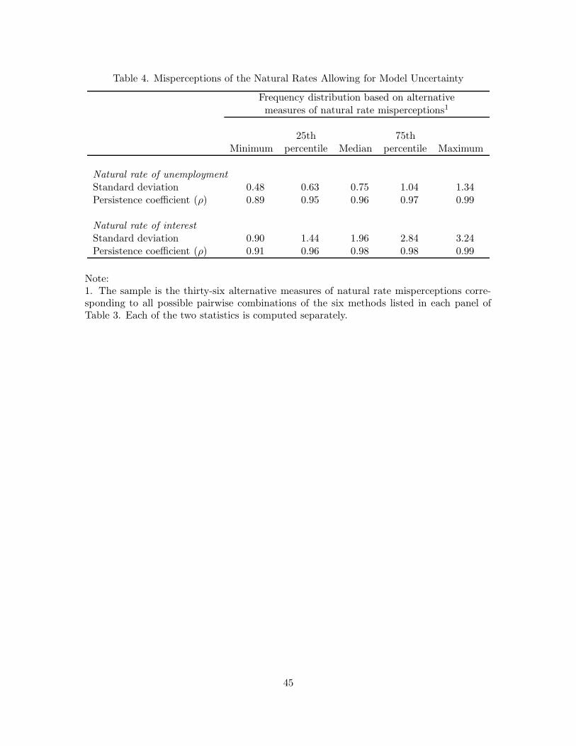
Table 4. Misperceptions of the Natural Rates Allowing for Model Uncertainty

Frequency distribution based on alternativemeasures of natural rate misperceptions1

25th 75thMinimum percentile Median percentile Maximum

Natural rate of unemploymentStandard deviation 0.48 0.63 0.75 1.04 1.34Persistence coefficient (ρ) 0.89 0.95 0.96 0.97 0.99

Natural rate of interestStandard deviation 0.90 1.44 1.96 2.84 3.24Persistence coefficient (ρ) 0.91 0.96 0.98 0.98 0.99

Note:1. The sample is the thirty-six alternative measures of natural rate misperceptions corre-sponding to all possible pairwise combinations of the six methods listed in each panel ofTable 3. Each of the two statistics is computed separately.

45

Table 5. Macroeocnomic Performance under Alternative Policy Rules

Rule parameter2 Standard deviation3 LossRule and (ω = 0.2,misperception index1 θf θπ θu θ∆u u− u∗ π ∆f (ψ = 0.05)Classic Taylor rules = 0 0.0 0.5 −1.0 0.0 0.81 2.14 2.83 1.84s = 1 0.0 0.5 −1.0 0.0 0.88 3.67 2.88 3.73s = 2 0.0 0.5 −1.0 0.0 1.01 6.11 3.38 8.85s = 3 0.0 0.5 −1.0 0.0 1.18 8.72 4.15 17.18

Revised Taylor rules = 0 0.0 0.5 −2.0 0.0 0.71 2.03 2.89 1.64s = 1 0.0 0.5 −2.0 0.0 0.77 4.13 2.91 4.32s = 2 0.0 0.5 −2.0 0.0 0.91 7.28 3.56 11.89s = 3 0.0 0.5 −2.0 0.0 1.09 10.57 4.59 24.36

Taylor rule optimized for s = 0s = 0 0.0 0.31 −3.81 0.0 0.61 2.05 2.83 1.54s = 1 0.0 0.31 −3.81 0.0 0.71 7.15 3.09 11.11s = 2 0.0 0.31 −3.81 0.0 0.94 13.64 4.54 38.94s = 3 0.0 0.31 −3.81 0.0 1.22 20.22 6.41 85.05

Taylor rule optimized for s = 1s = 0 0.0 1.37 −1.23 0.0 0.73 1.86 4.25 2.02s = 1 0.0 1.37 −1.23 0.0 0.79 2.07 4.90 2.56s = 2 0.0 1.37 −1.23 0.0 0.82 2.50 4.94 3.01s = 3 0.0 1.37 −1.23 0.0 0.86 3.05 5.11 3.76

Generalized rule optimized for s = 0s = 0 0.72 0.26 −1.83 −2.39 0.62 1.82 2.23 1.23s = 1 0.72 0.26 −1.83 −2.39 0.70 4.49 2.32 4.71s = 2 0.72 0.26 −1.83 −2.39 0.95 8.36 3.01 15.16s = 3 0.72 0.26 −1.83 −2.39 1.27 12.35 4.00 32.58

Generalized rule optimized for s = 1s = 0 0.97 0.39 −0.23 −5.39 0.66 1.94 2.45 1.40s = 1 0.97 0.39 −0.23 −5.39 0.66 1.95 2.42 1.40s = 2 0.97 0.39 −0.23 −5.39 0.66 2.08 2.40 1.50s = 3 0.97 0.39 −0.23 −5.39 0.66 2.32 2.40 1.71

Robust difference rules = ∞ 1.0 0.35 0.0 −5.96 0.66 2.01 2.49 1.46

Notes:1. s indexes the magnitude of policymakers’ misperception of the true natural rates.2. Parameters measure policymakers’ response to the lagged federal funds rate, the inflationgap, the unemployment gap, and the change in the unemployment rate, respectively.3. Unconditional standard deviation of the unemployment gap, the inflation rate, and thechange in the federal funds rate, respectively.

46

Table 6. Robust Policy Rule Parameters under Alternative Policymaker Preferences1

Loss parameters Rule parameter2 Standard deviationω ψ θπ θ∆u u− u∗ π ∆f0.5 0.05 0.57 −6.29 0.67 1.94 2.780.5 0.50 0.25 −3.56 0.82 2.22 1.770.5 5.00 0.13 −2.43 1.05 2.67 1.48

0.2 0.05 0.35 −5.96 0.66 2.01 2.490.2 0.50 0.17 −3.34 0.85 2.32 1.660.2 5.00 0.12 −2.34 1.09 2.76 1.46

0.1 0.05 0.24 −5.79 0.65 2.08 2.360.1 0.50 0.14 −3.25 0.87 2.38 1.620.1 5.00 0.11 −2.30 1.11 2.80 1.46

Notes:1. See Table 5 for definitions of parameters and performance measures.2. Parameters of the robust rule in equation (3) of the text.

47

Table 7. Performance under Optimized and under Robust Rules for Alternative Models

Loss when policy follows1

Robust Generalized Taylor rule optimized for s = 0Model rule True s = 0 True s = 1 True s = 2 True s = 3

Baseline 1.46 1.23 4.71 15.16 32.58New-Synthesis 0.63 0.56 0.69 1.02 1.56Accelerationist 5.13 2.19 2.53 3.54 5.24

Note:1. Loss as calculated by equation (12) in the text assuming ω = 0.2, ψ = 0.05.

48

Table 8. Robust Policy Rules across Alternative Models1

Rule Loss when true model is:Loss parameters parameter2 Baseline Accelerationist New synthesisω ψ θπ θ∆u model model model0.5 0.05 1.56 −7.13 2.89 5.45 1.120.5 0.50 0.84 −4.23 5.84 10.19 2.200.5 5.00 0.56 −3.21 24.21 32.06 9.61

0.2 0.05 1.28 −7.85 1.88 5.27 0.740.2 0.50 0.76 −4.41 4.60 9.73 1.840.2 5.00 0.54 −3.26 22.55 30.72 9.32

0.1 0.05 1.15 −8.19 1.53 5.14 0.600.1 0.50 0.72 −4.49 4.17 9.51 1.720.1 5.00 0.53 −3.28 21.98 30.22 9.23

Notes:1. See Table 5 for definitions of parameters and performance measures.2. Parameters of the robust rule (equation (3) in the text) chosen to minimize the expectedloss for the indicated values of the loss parameters, when the model is unknown and eachof the models is assigned equal likelihood of being the true model. Loss is calculated byequation (12) in the text.

49

Table 9: Estimates of the Natural Rate of Unemployment, 1995–2002

Council ofSurvey of Professional Congressional EconomicForecasters (real-time)1 Budget Office Advisers

Year Low Median High Real-Time2 Retrospective3 (real-time)4

1995 — — — 6.0 5.3 5.5–5.81996 5.00 5.65 6.00 5.8 5.2 5.71997 4.50 5.25 5.88 5.8 5.2 5.51998 4.50 5.30 5.80 5.8 5.2 5.41999 4.13 5.00 5.60 5.6 5.2 5.32000 4.00 4.50 5.00 5.2 5.2 5.22001 3.50 4.88 5.50 5.2 5.2 5.12002 3.80 5.10 5.50 5.2 5.2 4.9

Notes:1. Responses are those from the third-quarter in the indicated year.2. Estimates are from the The Budget and Economic Outlook published in the indicatedyear (usually in January).3. Estimates are from Congressional Budget Office (2002).4. Estimates are from the Economic Report of the President published in the year shown(usually in February) and reflect either explicit references to a NAIRU estimate, or, whenno explicit reference appears, the unemployment rate at the end of the long-term economicforecast presented in the report.

50

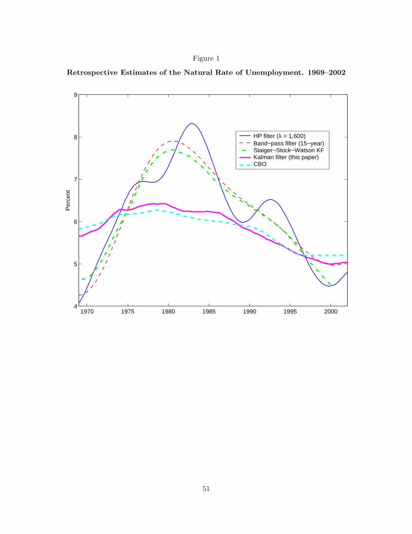
Figure 1

Retrospective Estimates of the Natural Rate of Unemployment. 1969–2002

1970 1975 1980 1985 1990 1995 20004

5

6

7

8

9

Per

cent

HP filter (λ = 1,600)Band−pass filter (15−year)Staiger−Stock−Watson KFKalman filter (this paper)CBO

51

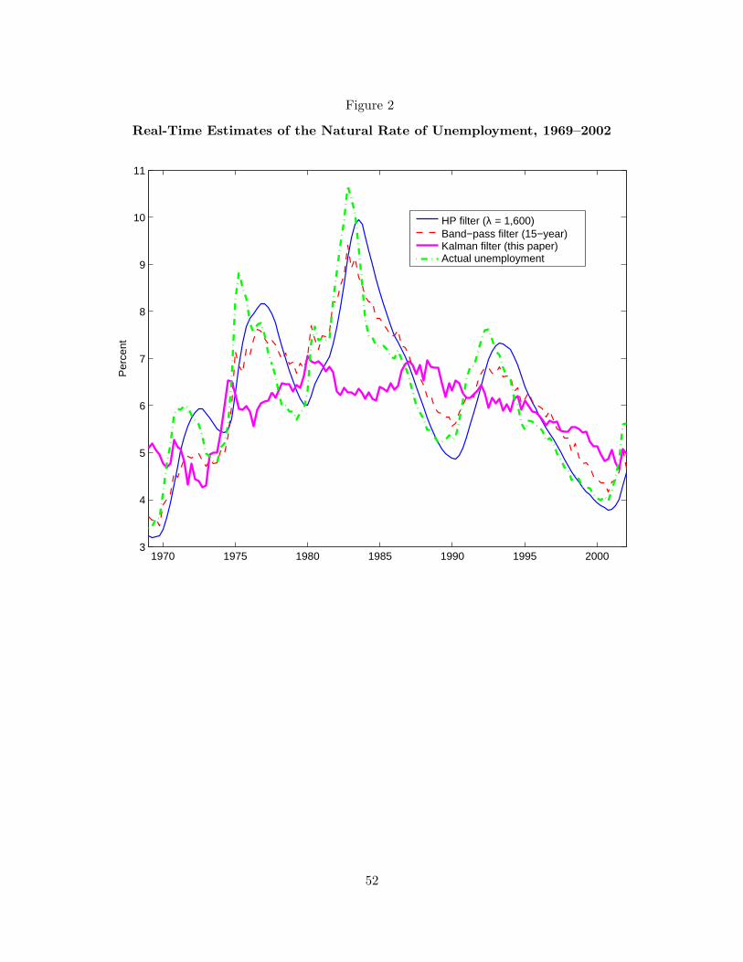
Figure 2

Real-Time Estimates of the Natural Rate of Unemployment, 1969–2002

1970 1975 1980 1985 1990 1995 20003

4

5

6

7

8

9

10

11

Per

cent

HP filter (λ = 1,600)Band−pass filter (15−year)Kalman filter (this paper)Actual unemployment

52

Figure 3

Retrospective Estimates of the Natural Rate of Interest, 1969–2002

1970 1975 1980 1985 1990 1995 2000−1

0

1

2

3

4

5

6

7

8

Per

cent

HP filter (λ = 1,600)Band−pass filter (15−year)Kalman filter (this paper)Laubach−Williams KF

53

Figure 4

Real-Time Estimates of the Natural Rate of Interest, 1969–2002

1970 1975 1980 1985 1990 1995 2000−4

−2

0

2

4

6

8

10

12

14

Per

cent

HP filter (λ = 1,600)Band−pass filter (15−year) Kalman filter (this paper) Laubach−Williams KF Actual real rate

54

Figure 5

Macroeconomic Performance of Taylor Rules forGiven Degrees of Natural Rate Misperceptions

0 0.5 1 1.5 2 2.5 31

2

4

8

SD

(lo

g sc

ale)

Inflation

S

Standard Taylor ruleRevised Taylor rule

0 0.5 1 1.5 2 2.5 30.5

0.75

1

1.25

SD

(lo

g sc

ale)

Unemployment Gap

S

Notes: The two panels show the asymptotic standard deviation of inflation and the un-employment gap (vertical axis, in percent) corresponding to the degree of misperceptionsregarding the natural rates, s (horizontal axis) when policy follows the original and revisedTaylor rules, reflected by the solid and dashed lines, respectively.

55

Figure 6

Optimal Policy Response Parameters under Taylor Rules forGiven Degrees of Natural Rate Misperceptions

0 0.5 1 1.5 2 2.5 30

0.5

1

1.5

2

S

θπ

0 0.5 1 1.5 2 2.5 3−4

−3

−2

−1

0

S

θu

Notes: The lines indicate the optimal choices of the parameters θπ and θu in the policy rule:ft = r∗t +πt + θπ(πt −π∗)+ θu(ut −u∗t ) for different degrees of misperceptions regarding thenatural rates, s.

56

Figure 7

Performance with Optimized and Robust Taylor Rules forGiven Degrees of Natural Rate Misperceptions

0 0.5 1 1.5 2 2.5 31

2

4

8

Inflation

S

SD

(lo

g sc

ale)

Optimized for s=0Optimized for s=1Robust rule

0 0.5 1 1.5 2 2.5 3.50

.75

1.00

1.25 Unemployment Gap

S

SD

(lo

g sc

ale)

0 0.5 1 1.5 2 2.5 32

3

4

5

6Change in Funds Rate

S

SD

(lo

g sc

ale)

0 0.5 1 1.5 2 2.5 31

2

4

8

Loss

log

scal

e

S

Notes: The three lines in each panel show the asymptotic standard deviations/loss (ver-tical axes) corresponding to the degree of misperceptions regarding the natural rates, s(horizontal axis) for three alternative policy rules: the Taylor rule (1) optimized with theassumption that s = 0 (solid lines); the Taylor rule (1) optimized with the assumption thats = 1 (dashed lines); and the robust rule (3) (dash-dot lines).

57

Figure 8

Optimal Policy Response Parameters under Generalized Policy Rules forGiven Degrees of Natural Rate Misperceptions

0 0.5 1 1.5 2 2.5 30.7

0.75

0.8

0.85

0.9

0.95

1θf

S0 0.5 1 1.5 2 2.5 3

0.25

0.3

0.35

0.4

0.45

S

θπ

0 0.5 1 1.5 2 2.5 3−2

−1.5

−1

−0.5

0

S

θu

0 0.5 1 1.5 2 2.5 3−6

−5

−4

−3

−2 θ∆(u)

S

Notes: The lines indicate the optimal choices of the parameters θf , θπ, θu and θ∆u in thepolicy rule: ft = θfft−1 + (1− θf )(r∗t + πt) + θπ(πt − π∗) + θu(ut − u∗t ) + θ∆u(ut − ut−1) fordifferent degrees of misperceptions regarding the natural rates, s.

58

Figure 9

Performance with Robust and Generalized Taylor Rules forGiven Degrees of Natural Rate Misperceptions

0 0.5 1 1.5 2 2.5 31

2

4

8

Inflation

S

SD

(lo

g sc

ale)

Optimized for s=0Optimized for s=1Robust rule

0 0.5 1 1.5 2 2.5 3.5

.75

1.0

1.25 Unemployment Gap

S

SD

(lo

g sc

ale)

0 0.5 1 1.5 2 2.5 32

3

4

5

6

S

SD

(lo

g sc

ale)

Change in Funds Rate

0 0.5 1 1.5 2 2.5 31

2

4

8

S

Loss

log

scal

e

Notes: The three lines in each panel show the asymptotic standard deviations/loss (verticalaxes) corresponding to the degree of misperceptions regarding the natural rates, s (hori-zontal axis) for three alternative policy rules: the generalized rule (2) optimized with theassumption that s = 0, (solid lines); the generalized rule (2) optimized with the assumptionthat s = 1 (dashed lines); and the robust rule (3) (dash-dot lines).

59

Figure 10

Efficient Policy Response Parameters under Generalized Taylor Rules forGiven Degrees of Natural Rate Misperceptions

0.7 0.8 0.9 1 −2

−1.5

−1

−0.5

0 θu

θf

S=0

S=1

Bayesian over [0,2]

S=2 Robust policy

Notes: The solid line traces the pairs of optimal choices of the parameters θf (horizontalaxis) and θu (vertical axis) for different known degrees of misperceptions shown in Figure10. Movements along the line in the northeast direction correspond to higher values ofs and the pairs corresponding to s = 0, 1, 2 are marked with an x. “Bayesian” indicatesthe optimal choices when the policymakers has a uniform prior about s on the [0,2] range.“Robust” indicates our simple difference rule.

60

Figure 11

Optimal Policy Response Parameters in New Synthesis Model forGiven Degrees of Natural Rate Misperceptions

0 0.5 1 1.5 2 2.5 31

1.05

1.1

1.15

1.2

S

θf

0 0.5 1 1.5 2 2.5 30.5

0.6

0.7

0.8

0.9

S

θπ

0 0.5 1 1.5 2 2.5 3−1.25

−1

−0.75

−0.5

−0.25

0 θu

S0 0.5 1 1.5 2 2.5 3

−2.2

−2

−1.8

−1.6

−1.4

−1.2

−1θ∆(u)

S

Notes: The lines indicate the optimal choices of the parameters θf , θπ, θu and θ∆u in theNew-Synthesis model when policy follows the rule: ft = θfft−1 +(1− θf)(r∗t +πt)+ θπ(πt −π∗) + θu(ut − u∗t ) + θ∆u(ut − ut−1) for different degrees of misperceptions regarding thenatural rates, s.

61

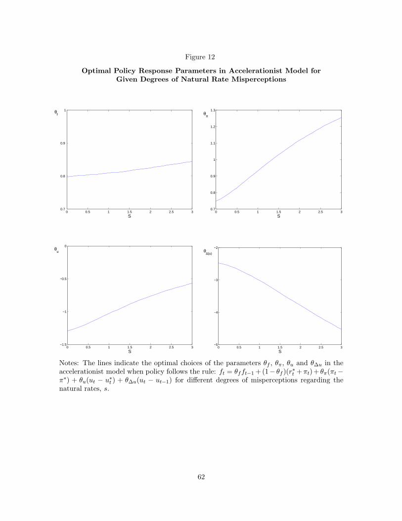
Figure 12

Optimal Policy Response Parameters in Accelerationist Model forGiven Degrees of Natural Rate Misperceptions

0 0.5 1 1.5 2 2.5 30.7

0.8

0.9

1

S

θf

0 0.5 1 1.5 2 2.5 30.7

0.8

0.9

1

1.1

1.2

1.3

S

θπ

0 0.5 1 1.5 2 2.5 3−1.5

−1

−0.5

0θ

u

S0 0.5 1 1.5 2 2.5 3

−5

−4

−3

−2θ

∆(u)

S

Notes: The lines indicate the optimal choices of the parameters θf , θπ, θu and θ∆u in theaccelerationist model when policy follows the rule: ft = θfft−1 +(1− θf )(r∗t +πt)+ θπ(πt −π∗) + θu(ut − u∗t ) + θ∆u(ut − ut−1) for different degrees of misperceptions regarding thenatural rates, s.

62

Figure 13

Misperceptions of Natural Rates Following an Unexpected Increase

0 2 4 60

0.5

1

1.5

R*

True valueReal−time est.

0 2 4 60

0.5

1

1.5

U*

0 2 4 60

0.2

0.4

0.6

0.8

1

1.2

Real−time R* Errors

Years0 2 4 6

0

0.2

0.4

0.6

0.8

1

1.2

Real−time U* Errors

Years

Notes: The top panels indicate the evolution of the true and perceived natural rate of inter-est (left) and unemployment (right) over time, following a series of unanticipated increasesin the natural rates which cumulate to 1.5 percentage points over a period of 10 quarters(2 1/2 years). The bottom panels trace the resulting evolution of misperceptions aboutthe natural rates over time. In all panels, we plot deviations from steady state values, inpercent.

63

Figure 14

Performance under Taylor Rules Following aMisperceived Increase in Natural Rates

0 1 2 3 4 5 6 7

0

1

2

3

4

5

6

7Inflation

Years

Classic Taylor RuleRevised Taylor Rule

0 1 2 3 4 5 6 70

0.2

0.4

0.6

0.8

1

1.2

1.4

1.6

Years

Unemployment Rate

True U*Real−time U* Est.Classic Taylor RuleRevised Taylor Rule

Notes: The two panels trace the evolution of inflation and unemployment (deviations fromsteady state values, in percentage points) in an economy subjected to the unexpected in-creases in the natural rates of interest and unemployment shown in Figure 13 for the classicand revised versions of the Taylor rule.

64

Figure 15

Performance under Optimized Generalized and Robust RulesFollowing a Misperceived Increase in Natural Rates

Optimized generalized rule

0 1 2 3 4 5 6 7

0

1

2

3

4

5

6

7Inflation

Years0 1 2 3 4 5 6 7

0

0.2

0.4

0.6

0.8

1

1.2

1.4

1.6

Years

Unemployment Rate

True U*Real−time U*Unemployment rate

Robust Rule

0 1 2 3 4 5 6 7

0

1

2

3

4

5

6

7Inflation

Years0 1 2 3 4 5 6 7

0

0.2

0.4

0.6

0.8

1

1.2

1.4

1.6

Years

Unemployment Rate

True U*Real−time U*Unemployment rate

Notes: The top and bottom panels trace the evolution of inflation and unemploymentin an economy subjected to the unexpected increases in the natural rates of interest andunemployment shown in Figure 13 for two alternative policies: The optimized generalizedrule for s = 0 (row 17 in Table 2) shown in the top panels, and the robust rule (row 25 inTable 2) in the bottom panels. In all panels, we plot deviations from steady state values,in percent.

65

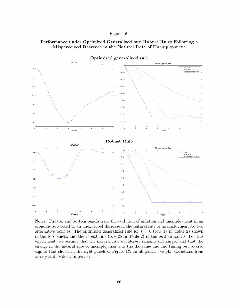
Figure 16

Performance under Optimized Generalized and Robust Rules Following aMisperceived Decrease in the Natural Rate of Unemployment

Optimized generalized rule

0 1 2 3 4 5 6 7

−6

−5

−4

−3

−2

−1

0

Inflation

Years0 1 2 3 4 5 6 7

−1.6

−1.4

−1.2

−1

−0.8

−0.6

−0.4

−0.2

0

Years

Unemployment Rate

True U*Real−time U*Unemployment rate

Robust Rule

0 1 2 3 4 5 6 7

−6

−5

−4

−3

−2

−1

0

Years

Inflation

0 1 2 3 4 5 6 7

−1.6

−1.4

−1.2

−1

−0.8

−0.6

−0.4

−0.2

0

Years

Unemployment Rate

True U*Real−time U*Unemployment rate

Notes: The top and bottom panels trace the evolution of inflation and unemployment in aneconomy subjected to an unexpected decrease in the natural rate of unemployment for twoalternative policies: The optimized generalized rule for s = 0 (row 17 in Table 2) shownin the top panels, and the robust rule (row 25 in Table 2) in the bottom panels. For thisexperiment, we assume that the natural rate of interest remains unchanged and that thechange in the natural rate of unemployment has the the same size and timing but reversesign of that shown in the right panels of Figure 13. In all panels, we plot deviations fromsteady state values, in percent.

66