the biosolids emissions assessment model (beam): a … · 2014-04-24 · emissions from canadian...
TRANSCRIPT

The Biosolids Emissions Assessment Model (BEAM): A Method for Determining Greenhouse Gas Emissions from Canadian Biosolids Management Practices
Final Report
July 2009
Prepared for:
Canadian Council of Ministers of the Environment 123 Main Street, Suite 360
Winnipeg, Manitoba Canada R3C 1A3
Prepared by:
SYLVIS 427 Seventh Street
New Westminster, British Columbia Canada V3M 3L2
Toll-Free: 1.800.778.1377 www.sylvis.com
PN 1432
Disclaimer: This report was prepared by SYLVIS Environmental for the Canadian Council of Ministers of
the Environment (CCME). This publication is a working paper only. It contains information which has
been prepared for, but not approved by, CCME. CCME is not responsible for the accuracy of the data
contained in the publication and does not warrant or necessarily share or affirm, in any way, any opinions
expressed therein.
© Canadian Council of Ministers of the Environment, 2009

THE BIOSOLIDS EMISSIONS ASSESSMENT MODEL (BEAM) JULY 2009 FINAL REPORT PAGE II
EXECUTIVE SUMMARY Biosolids management practices are evaluated based on environmental, economic and social impacts. A consideration of increasing importance is the impact of greenhouse gas (GHG) emissions from biosolids (treated sludge). The Canadian Council of Ministers of the Environment (CCME) retained the services of SYLVIS Environmental, and their project team, composed of Ned Beecher (Northeast Biosolids and Residuals Association), Dr. Sally Brown (University of Washington, College of Forest Resources), and Andrew Carpenter (Northern Tilth) who undertook a review of literature and leading GHG accounting and verification protocols, and developed a model for calculating GHG emissions from biosolids management. Using the model, GHG emissions estimates were calculated for nine biosolids management scenarios across Canada.
The literature review was completed to verify potential GHG sources and emission factors for biosolids and sludge management processes in the model development. Where possible, values, emission factors and assumptions were corroborated by multiple sources to ensure the use of the most current and accurate information possible.
A review of existing GHG accounting and verification protocols was completed to ensure the terminology and reporting methods adopted in the model were consistent with these protocols. Development of the model was based on leading protocols to facilitate the use of the model as a tool that is widely accepted as a verifiable method of determining carbon credits which can be sold or traded to offset the cost of biosolids management.
The model, termed the “Biosolids Emissions Assessment Model”, (BEAM) consists of 12 unit process calculator modules and an aggregating spreadsheet that calculates net GHG emissions based on the values determined within each applicable module.
The BEAM was developed to be flexible and user friendly and to facilitate use throughout Canada. The BEAM accomplishes this by:
• allowing the user to select only the unit process calculator modules that apply to their management practices;
• clearly highlighting within each calculator module the data required to generate a GHG emission value for each unit process;
• having the option to use default values that are used in the absence of user-provided data;
• locked calculator modules that are not input cells, thereby reducing calculation errors; and

THE BIOSOLIDS EMISSIONS ASSESSMENT MODEL (BEAM) JULY 2009 FINAL REPORT PAGE III
• having the flexibility to be easily revised based on new information gained through scientific research in the fields of GHG emissions and biosolids management.
The BEAM returns a net and per dry megagram (Mg) biosolids GHG emissions value based on user inputs and the use of default values as required. The BEAM, in following conventional GHG reporting and protocols, delineates emissions by Scope 1, 2 and 3 emissions; descriptions and examples of these emission scopes are provided within the final report.
A user guide was developed to assist jurisdictions using the BEAM. The user guide provides a step-by-step description of how to use the BEAM and includes captioned figures that show specific elements of the model. The user guide provides an explanation of how to review and interpret results. The appendices within the final report provide further explanation on the calculations and assumptions used in each BEAM unit process module.
The start and endpoints (boundaries) for the BEAM are from solids thickening at the wastewater treatment plant through to biosolids end use/disposal. Calculator tools were developed to determine GHG emissions from commonly used technologies within this segment of the process train (unit processes). Table 1 provides a summary of factors considered within each unit process module in the BEAM. The extensive lists of considerations for each unit process module demonstrate the level of detail involved in the development of the BEAM.
Table 1: Summary of considerations for unit process calculations.
Unit Process Considerations
Storage • mass of BOD in storage (kg/day) • aeration and electricity use (kWh/day) • depth of storage lagoon (m)
Solids Conditioning / Thickening
• volume of sludge thickened (m3/day) • sludge solids content (%) • thickening process • polymer use (kg/day) • electricity use (kWh/day)
Aerobic Digestion
• volume of sludge to digestion (m3/day) • sludge solids content (%) • volatile solids content (%) • volatile solids destruction (%) • electricity use (kWh/day) • fuel use, if needed (m3/day)

THE BIOSOLIDS EMISSIONS ASSESSMENT MODEL (BEAM) JULY 2009 FINAL REPORT PAGE IV
Anaerobic Digestion
• volume of sludge to digestion (m3/day) • sludge solids content (%) • volatile solids content (%) • volatile solids destruction (%) • biogas and methane yield (m3/day) • net electricity use/gain (kWh/day) • net fuel use/gain (m3/day) • flaring and fugitive emissions of methane (%)
Dewatering
• volume of sludge thickened (m3/day) • sludge solids content (%) • thickening process • polymer use (kg/day) • electricity use (kWh/day)
Thermal Drying
• mass of sludge to be dried (Mg/day) • sludge solids content before and after drying (%) • electricity use (kWh/day) • fuel use (m3/day)
Alkaline Stabilization
• mass of sludge to be stabilized (Mg/day) • sludge solids content (%) • degree of stabilization • amount of alkaline material added (Mg/day) • lime is a by-product (yes/no) • electricity use (kWh/day) • fuel use (m3/day)
Composting
• mass of sludge to be composted (Mg/day) • sludge solids content (%) • sludge density (kg/m3) • processing prior to composting • nutrient content of sludge • fertilizer replacement (yes/no) • amount of amendment used (volumetric ratio) • amendment grinding (yes/no) • density of amendment (kg/m3) • type of composting equipment • biofilter (yes/no) • fuel use (L-diesel/day) • electricity (kWh/day)

THE BIOSOLIDS EMISSIONS ASSESSMENT MODEL (BEAM) JULY 2009 FINAL REPORT PAGE V
Landfill Disposal
• mass of sludge to be landfilled (Mg/day) • sludge solids content (%) • sludge density (kg/m3) • processing prior to landfilling • nutrient content of sludge • methane correction factor • quality of daily cover • methane captured (%) • methane used for generating electricity (%) • Degradable organic carbon that will decompose in a
landfill (DOCf) (%) • Degradable organic carbon that will degrade prior to
methane capture (%)
Combustion
• mass of sludge to be incinerated (Mg/day) • sludge solids content (%) • processing prior to incineration • nitrogen/nutrient content of sludge • type of incinerator • energy recovered as electricity and/or heat (%) • disposition/recycling of ash • urea-based selective noncatalytic reduction emissions
system (yes/no) • temperature of combustion • net fuel use/gain, including afterburner fuel requirements
in multiple hearth incineration (m3/day) • net electricity use/gain (kWh/day)
Land Application
• mass of biosolids to be land applied (Mg/day) • biosolids solids content (%) • biosolids density (kg/m3) • processing prior to land application • nutrient content of biosolids • calcium carbonate equivalence (%) • fertilizer replacement (yes/no) • lime replacement (yes/no) • lime is a by-product (yes/no) • biosolids storage time prior to land application (days) • texture of soils, fine, coarse (%) • fuel use (L-diesel/day)
Transportation • fuel use for transportation of biosolids or sludge • biodiesel use (% of total fuel)
The BEAM does not include calculations for emissions from emerging/pilot technologies (e.g. plasma oxidation); GHG associated with infrastructure construction; and GHG emissions from upstream wastewater processes (e.g. wastewater conveyance). Emissions from septic tanks and the pumping and management of septage (including its direct land application or

THE BIOSOLIDS EMISSIONS ASSESSMENT MODEL (BEAM) JULY 2009 FINAL REPORT PAGE VI
transportation to a wastewater treatment facility) are also not within the boundaries of the BEAM.
The BEAM was developed to be applicable to a wide variety of biosolids management scenarios. Nine Canadian jurisdictions provided “real-world” technical data from their biosolids management programs and these data were used in the development and validation of the BEAM. The nine jurisdictions were selected from an initial list of over forty Canadian cities. Selection of the participating jurisdictions was based upon a variety of biosolids management practices, regional representation, leadership in biosolids management, and their commitment to participate in model development. The scenarios cover land use, composting, incineration and landfilling, with or without energy recovery, including anaerobic digestion. While biosolids management from lagoons is not addressed in the nine scenarios, it is still covered by the model.
Table 2 summarizes the scenarios and the unit processes that were used in the BEAM GHG determinations. Net and per dry Mg (tonne) biosolids GHG emissions from these scenarios are provided in Table 3. A summary of net GHG emissions on a per dry Mg (tonne) biosolids basis is presented graphically in Figure 1.
Table 2: Biosolids management scenario unit process summary.
Scenario Jurisdiction Unit Processes Considered in BEAM Calculations
1 Thunder Bay1
• primary clarifier thickening
• dissolved air floatation secondary thickening
• anaerobic digestion
• centrifuge dewatering
• transportation
• biosolids/soil mix to cover on landfill (final cover, see text)
2 Incineration scenario2
• primary gravity thickening
• rotary press dewatering
• incineration (760°C) with heat recovery
• ash recycling
3 Laval
• primary thickening
• anaerobic solids storage of liquid sludge
• rotary press dewatering
• landfill a portion (14%) of dewatered cake
• thermal drying and pelletization
• transportation
• cement kiln incineration of most biosolids (1460°C)
4 Windsor • primary solids gravity thickening

THE BIOSOLIDS EMISSIONS ASSESSMENT MODEL (BEAM) JULY 2009 FINAL REPORT PAGE VII
• high speed centrifuge dewatering
• thermal drying and pelletizing
• agricultural land application
5 Moncton
• primary clarifier thickening
• centrifuge dewatering / polymer addition
• alkaline stabilization
• composting
• compost use
6 Vancouver
• primary gravity thickening
• dissolved air floatation secondary thickening
• anaerobic digestion
• digester gas utilization (electricity production)
• centrifuge dewatering
• transportation
• mine site applications
7 Halifax
• primary clarifier thickening
• anaerobic digestion
• digester gas utilization (heat production)
• Fournier press dewatering
• stabilization using recycled alkaline sources (e.g. cement kiln dust)
• transportation
• agricultural land application
8 Nanaimo
• primary and secondary gravity thickening
• aerobic digestion
• centrifuge dewatering
• transportation
• silvicultural land application
9 Halton
• dissolved air floatation thickening and polymer addition
• anaerobic digestion
• liquid biosolids storage
• belt filter press dewatering
• transportation
• liquid and dewatered biosolids agricultural applications
1. Landfilling of sludge/biosolids is only covered partially in Scenario 3 where Laval landfills a part (14%) of the primary sludge. In Scenario 1, Thunder Bay sends anaerobically digested biosolids at a landfill, where it is used as a blended soil product applied on the surface of the landfill for final cover. Hence it is more related to land application scenarios.

THE BIOSOLIDS EMISSIONS ASSESSMENT MODEL (BEAM) JULY 2009 FINAL REPORT PAGE VIII
2. This scenario corresponds to one of the seven Canadian cities that operate sludge incinerators.

Biosolids Management
Scenario1Jurisdiction WWTP Name Population
Served Wastewater
Treated (MLD)
Net GHG Emissions (Mg CO2
equivalents / year)
GHG Emissions Mg CO2eq/ Mg
dry solids
1 Thunder Bay Atlantic Avenue 100,000 70 1,462 0.09
2 Incineration Scenario - - 295 19,608 1.63
3 Laval La Pinière 271,633 254 10,277 1.02
4 Windsor Lou Romano 181,348 161 2,427 0.22
5 Moncton GMSC 125,000 79 1,123 0.18
6 Vancouver Annacis Island 980,000 436 –1,868 –0.16
7 Halifax Mill Cove 54,000 27 –875 –0.15
8 Nanaimo French Creek 25,000 10 177 0.11
9 Halton Burlington Skyway 165,000 96 –531 –0.18
HE BIOSOLIDS EMISSIONS ASSESSMENT MODEL (BEAM) JULY 2009 FINAL REPORT PAGE IX
Table 3: Summary of GHG emissions from the biosolids management scenarios.
1 See Table 2 for scenario description.
T

A summary of net GHG emissions on a per dry Mg biosolids basis are presented graphically in Figure 1.
Figure 1: Summary of net GHG emissions on a per dry Mg (tonne) biosolids basis. (Refer to Table 2 for descriptions of each scenario.)
The BEAM outputs indicate higher emissions from two jurisdictions, the incineration scenario and Laval. In the incineration scenario, the burning of dewatered sludge at relatively low temperature (760°C) produces significant N2O emissions, according to Japanese studies and the algorithm used in the model. For Laval, N2O emissions remain low, due to high temperatures of combustion, while CO2 emissions from heat drying at the WWTP are entirely offset by fuel savings at the cement kiln. Laval’s emissions are mainly associated with anaerobic storage of liquid sludge and landfilling a portion (14%) of the primary sludge cake, both of which result in significant CH4 emissions.
Conversely it appears that net GHG neutrality or offsets can be obtained through land application/surface cover. It is due to less methane and N2O emissions and also to carbon sequestration in soil and reduced use of chemical fertilizers to promote plant growth.
Interestingly, biosolids transportation distances generally have little impact on GHG emissions from biosolids management. Although Metro Vancouver hauls their biosolids a relatively long distance to mine application sites, they have one of the lowest GHG emissions totals on a per dry tonne biosolids basis (negative value). In some jurisdictions, polymer use in thickening / conditioning is a greater source of GHGs than transportation, due to the GHG intensive nature of their industrial production.

THE BIOSOLIDS EMISSIONS ASSESSMENT MODEL (BEAM) JULY 2009 FINAL REPORT PAGE II
The results presented here are best estimates based on the current state of knowledge regarding GHG emissions from biosolids management. However, accuracy may vary according to some general factors including the use of default values as opposed to local or regional data, and assumptions made with respect to the biosolids management scenarios. In general, there is more known about sources and emissions relating to processes which release carbon dioxide (CO2), followed be methane (CH4) and nitrous oxide (N2O). The understanding of these three GHGs is inversely related to the relative importance of the GHGs; N2O and CH4 are 310 and 21 times more potent GHGs than CO2 respectively. Thus, as research progresses, particularly with respect to N2O and CH4, the model is amenable to revising default values and emission factors to improve overall model accuracy.
Identification of the incineration scenario and Laval management practices as the largest GHG emission scenarios prompted an investigation into process modifications that could decrease GHG emissions. The BEAM was used to evaluate the changes in biosolids processing and management. Modification of the incineration scenario focused on increasing the standard burn temperature of their fluidized bed incinerators from 760°C to 800°C. Areas for modifying the Laval scenario included the implementation of aerobic as opposed to anaerobic storage and composting the portion of dewatered biosolids which is currently landfilled.
Implementation of these modifications to the Laval and the incineration scenarios indicates a decrease in estimated GHG emissions from each modified management practice (Figure 2). Greenhouse gas emissions were decreased in the incineration scenario from 1.63 to 1.09 Mg CO2eq/Mg dry biosolids, due to reduced N2O emission from the incinerators. Increased fuel and electricity use associated with an increase in standard burn temperature were considered for the incineration scenario and found to have minimal impact on the net GHG emissions.
Greenhouse gas emissions from the Laval scenario were decreased from 1.01 to 0.22 Mg CO2eq/Mg dry biosolids, due largely to net negative (i.e. carbon credit generating) emissions from compost used as opposed to landfilling the equivalent volume of primary sludge. Compost use results in increased carbon sequestration and the displacement of chemical fertilizers and removal of the sludge from landfilling mitigates CH4 emissions associated with landfill disposal. Additionally, the elimination of CH4 emissions from anaerobic storage were mitigated by changing to aerobic storage. Figure 2 illustrates the potential GHG reductions predicted by the BEAM for these process modifications.

THE BIOSOLIDS EMISSIONS ASSESSMENT MODEL (BEAM) JULY 2009 FINAL REPORT PAGE III
Figure 2: Potential GHG reductions through process modifications.
Results highlight the usefulness of the BEAM as a tool for biosolids generators to estimate the impacts that process modifications can have on GHG emissions. Opportunities to reduce GHG emissions from the remaining seven scenarios are discussed qualitatively in the report. Examples of these opportunities include:
• increasing energy efficiency in processes that require electricity and fossil fuels;
• digester gas capture and utilization to offset purchased energy requirements; and
• increasing land application to obtain credits through carbon sequestration and displacement of chemical fertilizers.
The BEAM will be useful to wastewater treatment plant operators and biosolids managers as it:
• is designed to enable the calculation of GHG emissions from multiple management scenarios through the use of unit process calculators;
• isolates and summarizes the net emissions from each unit process, so that the user can clearly see which processes are the largest GHG contributors;

THE BIOSOLIDS EMISSIONS ASSESSMENT MODEL (BEAM) JULY 2009 FINAL REPORT PAGE IV
• allows the user to evaluate other unit processes they employ or are considering, so that their impact on overall GHG emissions can be estimated;
• can be used to calculate existing or potential carbon credits, which will become marketable as carbon trading systems develop, and facilitate opportunities for cost recovery or revenue generation from biosolids management programs.
The BEAM provides estimates of emissions for the solids management train that can be added to estimates for the wastewater treatment process to establish an overall estimate for the entire operation. The BEAM could serve as an important tool in the identification of opportunities for GHG mitigation measures and offset potentials in biosolids management that could serve as a cost recovery or revenue generation mechanism in emerging carbon markets. As market incentives for GHG emissions reductions develop further, documentation using BEAM, combined with an independent verification step, could lead to the generation of marketable carbon credits.

THE BIOSOLIDS EMISSIONS ASSESSMENT MODEL (BEAM) JULY 2009 FINAL REPORT PAGE V
TABLE OF CONTENTS
1 Introduction ........................................................................................................................ 1
1.1 Project Approach ......................................................................................................... 1
2 Report Organization........................................................................................................... 2
3 Summary of Tasks ............................................................................................................. 3
3.1 Literature Review......................................................................................................... 3
3.2 Review of Leading GHG Accounting and Verification Protocols ................................. 3
3.3 Background Review of Canadian Biosolids Management Practices ........................... 4
3.4 Method Development and the BEAM .......................................................................... 5
3.4.1 BEAM Overview...................................................................................................... 6
4 Jurisdictional Biosolids Management Options and GHG Emissions............................ 7
4.1 Jurisdiction Summaries and Results............................................................................ 9
4.1.1 Thunder Bay – Scenario 1 ...................................................................................... 9
4.1.2 Incineration – Scenario 2 ...................................................................................... 11
4.1.3 Laval – Scenario 3 ................................................................................................ 12
4.1.4 Windsor – Scenario 4............................................................................................ 14
4.1.5 Moncton – Scenario 5 ........................................................................................... 16
4.1.6 Metro Vancouver – Scenario 6.............................................................................. 17
4.1.7 Halifax – Scenario 7 .............................................................................................. 19
4.1.8 Regional District of Nanaimo – Scenario 8 ........................................................... 20
4.1.9 Halton – Scenario 9............................................................................................... 21
4.1.10 Edmonton.............................................................................................................. 23
5 BEAM User Guide............................................................................................................. 26

THE BIOSOLIDS EMISSIONS ASSESSMENT MODEL (BEAM) JULY 2009 FINAL REPORT PAGE VI
6 Conclusions and Recommendations ............................................................................. 26
6.1 Recommendations..................................................................................................... 27
7 References........................................................................................................................ 28
8 Review of Literature ......................................................................................................... 36
8.1 Scope of Reviewed Literature.................................................................................... 36
8.2 Potential GHG Debits from Biosolids Management Scenarios .................................. 37
8.2.1 Carbon dioxide emissions ..................................................................................... 37
8.2.2 Methane emissions ............................................................................................... 39
8.2.3 Nitrous oxide emissions ........................................................................................ 39
8.3 Greenhouse gas emissions from unit processes....................................................... 39
8.3.1 Lagoons ................................................................................................................ 40
8.3.2 Conditioning & Thickening .................................................................................... 41
8.3.3 Aerobic digestion................................................................................................... 41
8.3.4 Anaerobic digestion............................................................................................... 42
8.3.4.1 Combustion of Digester Gas......................................................................... 42
8.3.5 Dewatering ............................................................................................................ 43
8.3.6 Thermal drying ...................................................................................................... 43
8.3.7 Alkaline stabilization.............................................................................................. 44
8.3.8 Composting ........................................................................................................... 44
8.3.8.1 Carbon dioxide emissions from energy consumption for composting .......... 45
8.3.8.2 Methane emissions from composting ........................................................... 45
8.3.8.3 Nitrous oxide emissions from composting .................................................... 46
8.3.8.4 Biofilters ........................................................................................................ 49
8.3.9 Landfilling.............................................................................................................. 49

THE BIOSOLIDS EMISSIONS ASSESSMENT MODEL (BEAM) JULY 2009 FINAL REPORT PAGE VII
8.3.9.1 Carbon dioxide emissions............................................................................. 49
8.3.9.2 Methane emissions....................................................................................... 49
8.3.9.3 Methane emissions – landfill climate ............................................................ 50
8.3.9.4 Methane emissions – volatile solids reduction.............................................. 51
8.3.9.5 Methane emissions – Landfill gas capture.................................................... 53
8.3.9.6 Methane emissions – using biosolids as cover material............................... 57
8.3.9.7 Nitrous oxide emissions................................................................................ 57
8.3.10 Combustion ........................................................................................................... 58
8.3.10.1 Carbon dioxide emissions from incineration of biosolids .............................. 58
8.3.10.2 Methane emissions from incineration ........................................................... 60
8.3.10.3 Nitrous oxide emissions from incineration .................................................... 60
8.3.11 Land application.................................................................................................... 63
8.3.11.1 Carbon dioxide emissions from land application .......................................... 63
8.3.11.2 Methane emissions from land application..................................................... 64
8.3.11.3 Nitrous oxide emissions - agronomic rates................................................... 64
8.3.11.4 Nitrous oxide emissions – climate and soil ................................................... 65
8.3.11.5 Nitrous oxide emissions - higher rates of land application............................ 68
8.3.11.6 Timing of emissions from land application.................................................... 68
8.3.11.7 Nitrous oxide emissions - incorporation or topdressing ................................ 69
8.3.11.8 Nitrous oxide emissions – biosolids type ...................................................... 69
8.3.11.9 Impact of C:N ratio on N2O emissions .......................................................... 70
8.3.11.10 Nitrous oxide emissions - storage ................................................................ 70
8.4 Potential GHG Credits from Biosolids Management Scenarios................................. 73
8.4.1 Land application and compost use for fertilizer replacement ................................ 73

THE BIOSOLIDS EMISSIONS ASSESSMENT MODEL (BEAM) JULY 2009 FINAL REPORT PAGE VIII
8.4.2 Tapping the energy value of biosolids................................................................... 74
8.4.3 Credits for use of incinerator ash .......................................................................... 75
8.4.4 Sequestering carbon in soils and landfills ............................................................. 76
9 Review of Greenhouse Gas Accounting Protocols ...................................................... 80
9.1 Protocols for GHG Emissions Accounting ................................................................. 80
9.1.1 IPCC Protocol ....................................................................................................... 80
9.1.2 Clean Development Mechanism (CDM)................................................................ 82
9.1.3 The Greenhouse Gas Protocol ............................................................................. 82
9.1.4 ISO 14064............................................................................................................. 83
9.1.5 California Climate Action Registry (CCAR) ........................................................... 83
9.1.6 The Climate Registry (TCR).................................................................................. 83
9.1.7 National Inventories .............................................................................................. 85
9.2 Verification Programs ................................................................................................ 87
9.2.1 ISO 14065............................................................................................................. 87
9.2.2 The Climate Registry General Verification Protocol 2008..................................... 87
9.2.3 American National Standards Institute (ANSI) ...................................................... 87
9.2.4 Reliance on accounting protocols ......................................................................... 88
9.2.5 Canadian federal standards .................................................................................. 89
9.2.6 Protocols specific to wastewater treatment........................................................... 89
9.2.7 Biosolids management GHG emissions inventory projects .................................. 90
9.2.8 How does this relate to Life Cycle Analysis (LCA)? .............................................. 91
9.2.9 Critical issues in developing GHG emission protocols.......................................... 91
10 Review of Current Management Practices Across Canada ......................................... 94
11 Developing the BEAM.................................................................................................... 103

THE BIOSOLIDS EMISSIONS ASSESSMENT MODEL (BEAM) JULY 2009 FINAL REPORT PAGE IX
11.1 BEAM Development ................................................................................................ 103
11.2 BEAM General Principles ........................................................................................ 103
11.3 Critical issues in developing GHG emission protocols............................................. 104
11.4 General Assumptions .............................................................................................. 105
11.5 Comparison of the BEAM to Existing Methodologies .............................................. 106
11.6 Accuracy Estimates ................................................................................................. 107
11.7 Negligible Emissions................................................................................................ 108
11.8 Unit Process Information ......................................................................................... 109
11.8.1 Storage Lagoons................................................................................................. 112
11.8.2 Storage Tanks..................................................................................................... 112
11.8.3 Conditioning & Thickening .................................................................................. 112
11.8.4 Aerobic Digestion................................................................................................ 113
11.8.5 Anaerobic Digestion............................................................................................ 114
11.8.6 Combustion of Digester Gas ............................................................................... 114
11.8.7 Dewatering .......................................................................................................... 115
11.8.8 Alkaline Stabilization ........................................................................................... 115
11.8.9 Composting ......................................................................................................... 115
11.8.10 Biofiltration .......................................................................................................... 117
11.8.11 Landfill Disposal .................................................................................................. 117
11.8.12 Combustion ......................................................................................................... 118
11.8.13 Use of ash for cement manufacture .................................................................... 119
11.8.14 Land application questions.................................................................................. 119
11.8.15 Credits associated with biosolids applications .................................................... 123
12 BEAM Calculation Details.............................................................................................. 126

THE BIOSOLIDS EMISSIONS ASSESSMENT MODEL (BEAM) JULY 2009 FINAL REPORT PAGE X
12.1 Storage .................................................................................................................... 128
12.1.1 Critical GHG Emissions Factors.......................................................................... 128
12.1.2 Relevant Equations............................................................................................. 129
12.1.3 Assumptions & Discussion.................................................................................. 130
12.2 Conditioning & Thickening ....................................................................................... 131
12.2.1 Critical GHG Emissions Factors.......................................................................... 131
12.2.2 Relevant Equations............................................................................................. 131
12.2.3 Assumptions & Discussion.................................................................................. 132
12.3 Aerobic Digestion..................................................................................................... 133
12.3.1 Critical GHG Emissions Factors.......................................................................... 133
12.3.2 Relevant Equations............................................................................................. 133
12.3.3 Assumptions & Discussion.................................................................................. 134
12.4 Anaerobic Digestion................................................................................................. 135
12.4.1 Critical GHG Emissions Factors.......................................................................... 135
12.4.2 Relevant Equations............................................................................................. 136
12.4.3 Assumptions & Discussion.................................................................................. 138
12.5 Dewatering............................................................................................................... 140
12.5.1 Critical GHG Emissions Factors.......................................................................... 140
12.5.2 Relevant Equations............................................................................................. 140
12.5.3 Assumptions & Discussion.................................................................................. 141
12.6 Thermal Drying ........................................................................................................ 141
12.6.1 Critical GHG Emissions Factors.......................................................................... 141
12.6.2 Relevant Equations............................................................................................. 141
12.6.3 Assumptions & Discussion.................................................................................. 142

THE BIOSOLIDS EMISSIONS ASSESSMENT MODEL (BEAM) JULY 2009 FINAL REPORT PAGE XI
12.7 Alkaline Stabilization................................................................................................ 143
12.7.1 Critical GHG Emissions Factors.......................................................................... 143
12.7.2 Relevant Equations............................................................................................. 143
12.7.3 Assumptions & Discussion.................................................................................. 145
12.8 Composting.............................................................................................................. 145
12.8.1 Critical GHG Emissions Factors.......................................................................... 145
12.8.2 Relevant Equations............................................................................................. 146
12.8.3 Assumptions & Discussion.................................................................................. 150
12.9 Landfill Disposal....................................................................................................... 153
12.9.1 Critical GHG Emissions Factors.......................................................................... 153
12.9.2 Relevant Equations............................................................................................. 154
12.9.3 Assumptions & Discussion.................................................................................. 157
12.10 Combustion (Incineration)........................................................................................ 158
12.10.1 Critical GHG Emissions Factors.......................................................................... 158
12.10.2 Relevant Equations............................................................................................. 159
12.10.3 Assumptions & Discussion.................................................................................. 163
12.11 Land application....................................................................................................... 166
12.11.1 Critical GHG Emissions Factors.......................................................................... 166
12.11.2 Relevant Equations............................................................................................. 167
12.11.3 Assumptions & Discussion.................................................................................. 172
12.12 Transportation.......................................................................................................... 175
12.12.1 Critical GHG Emissions Factors.......................................................................... 176
12.12.2 Relevant Equation............................................................................................... 177
12.12.3 Assumptions & Discussion.................................................................................. 177

THE BIOSOLIDS EMISSIONS ASSESSMENT MODEL (BEAM) JULY 2009 FINAL REPORT PAGE XII
LIST OF TABLES
Table 1: Summary of considerations for unit process calculations..............................................iii
Table 2: Biosolids management scenario unit process summary. ..............................................vi
Table 3: Summary of GHG emissions from the biosolids management scenarios. ....................ix
Table 4: Short-listed jurisdictions for method development......................................................... 5
Table 5: Participating jurisdictions – summary of general information. ....................................... 8
Table 6: Summary of GHG emissions from the biosolids management scenarios. .................. 24
Table 7: Summary of research reporting N2O and CH4 emissions from composting operations.................................................................................................................... 48
Table 8: Collection efficiency for various cover reported in Spokas et al. (2006)...................... 55
Table 9: Collection Efficiency for Various Covers Reported in Borjesson et al. (2007)............ 55
Table 10: Impact of delays in collecting gas from newer landfill cells. ...................................... 57
Table 11: Rates of N2O emissions from different types of combusted biosolids. ...................... 61
Table 12: Land application of agronomic rate limits or guidance by province. .......................... 67
Table 13: Summary of research reporting N2O emissions from soils and treated soils............. 71
Table 14: Comparison of constituents in cement and sludge ash. ............................................ 75
Table 15: Comparison of greenhouse gas accounting protocols. ............................................. 86
Table 16: Summary of biosolids scenarios and corresponding generators............................... 95
Table 17: Detailed information for biosolids generators. ........................................................... 98
Table 18: Negligible GHG sources. ......................................................................................... 108
LIST OF FIGURES
Figure 1: Summary of net GHG emissions on a per dry Mg (tonne) biosolids basis.................... i
Figure 2: Potential GHG reductions through process modifications............................................iii
Figure 3: Summary of net GHG emissions on a per dry Mg biosolids basis. ............................ 25

THE BIOSOLIDS EMISSIONS ASSESSMENT MODEL (BEAM) JULY 2009 FINAL REPORT PAGE XIII Figure 4: Landfill cell and ambient temperature data (Lefebvre et al., 2000). ........................... 50
Figure 5: Volatile solids destruction versus time in anaerobic digestion (Metcalf & Eddy, 2002). ................................................................................................................ 51
Figure 6: Schematic of a wastewater treatment plant. ............................................................ 110
Figure 7: Unit process diagram. .............................................................................................. 111
LIST OF APPENDICES
Appendix One: Review of Literature
Appendix Two: Review of Greenhouse Gas Accounting Protocols
Appendix Three: Review of Current Canadian Biosolids Management Practices
Appendix Four: BEAM Development
Appendix Five: BEAM Calculation Development

THE BIOSOLIDS EMISSIONS ASSESSMENT MODEL (BEAM) JULY 2009 FINAL REPORT PAGE 1
1 INTRODUCTION
Biosolids generators evaluate the feasibility of biosolids management practices based on a number of environmental, economic, logistical and social criteria. These criteria often reflect a combination of the current understanding of biosolids management and generator-specific core values and objectives, and can include regulatory compliance; capital, operating and maintenance costs; interdepartmental synergies and public acceptance. Traditional environmental criteria include the protection of water resources, plants and animals; and odour abatement.
Concerns regarding climate change and the likelihood of more stringent greenhouse gas (GHG) emission regulations has resulted in biosolids generators interested in evaluating biosolids management projects, in part, based on the potential to minimize GHG emissions. In addition to being an environmental criterion, there are economic and social implications to considering GHG emission impacts. As GHG offset markets emerge, projects that sequester carbon and generate offsets could serve as a cost recovery or revenue generating mechanism. The potential impacts of GHG emissions on our climate are “top of mind” concerns in contemporary society; projects that seek to minimize these impacts promote corporate social responsibility and can increase public acceptance.
Biosolids are a significant organic residual that requires responsible management. Canadian biosolids generators produce approximately 2.5 million bulk tonnes of biosolids annually – quantities comparable in magnitude to other residuals including household waste and green waste (e.g. leaves and yard trimmings). While methodologies exist for determining GHG emissions from management of other organic residuals, there is a dearth of analogous information for biosolids management.
The Canadian Council of Ministers of the Environment (CCME) identified this knowledge gap and has pursued the development of a model for quantifying GHG emissions from biosolids management practices. The intent of the “Biosolids Emissions Assessment Model”, or “BEAM”, is to provide Canadian biosolids generators with a model for evaluating GHG emissions from current and proposed biosolids management practices.
1.1 Project Approach
The project was undertaken in sequential stages. The first stage involved a literature and background review. The literature review involved a synthesis of GHG emissions from possible unit processes associated with solids processing and biosolids management. The literature review also included a review of leading GHG accounting and verification protocols. The background review involved a summary of biosolids management practices currently implemented by Canadian jurisdictions.

THE BIOSOLIDS EMISSIONS ASSESSMENT MODEL (BEAM) JULY 2009 FINAL REPORT PAGE 2 The information gathered from the literature formed the basis for the development stage of the project. The BEAM and data request spreadsheets were developed. The BEAM and data spreadsheets are delineated by unit process modules, thus providing flexibility in use and increased applicability. Augmenting the BEAM and data spreadsheets a user guide to assist biosolids generators in using the BEAM and associated spreadsheets was developed.
The CCME identified ten biosolids management scenarios for GHG emissions calculations. These scenarios include the majority of biosolids management options currently employed in Canada. The goal of the background review of biosolids management in Canada was to identify jurisdictions engaged in these prioritized management practices, and have them assist in method development by providing information and data from their operations. Ten jurisdictions were identified and were provided relevant data request spreadsheets. This information was used to populate the corresponding unit process modules within the BEAM to quantify net GHG emissions from the specified biosolids management scenario provided by each jurisdiction.
2 REPORT ORGANIZATION
In the development of the BEAM, substantial background and review work was undertaken. Section 3 provides a summary of the work completed in the literature and background review, as well as the method development. Reports containing the literature and background reviews and details on the method development were prepared over the course of the project. The reader is referred to respective appendices (Sections 8-11) contained in this report, under continuous pagination, for details related to the literature review, overview of Canadian biosolids management practices and development of the BEAM.
An important aspect of method development was the application of “real-life” data to the BEAM corresponding to the biosolids management scenarios. Section 3.3 discusses the selection of ten Canadian jurisdictions to participate in this stage of the project. This section provides summaries of the participating jurisdictions’ biosolids management practices and preliminary results of their GHG emissions from specific biosolids management practices.
Section 5 introduces the user guide that supports the BEAM. The user guide provides a stepwise explanation of how to use the BEAM. The BEAM will be used by a wide range of professionals with varying degrees of knowledge related to biosolids and GHG emissions. As such, sufficient detail is provided in the user guide to enable those with limited knowledge on these topics to use the BEAM to generate meaningful data on GHG emissions from their biosolids management practices. This increases the applicability of the BEAM to a greater number of biosolids generators across Canada.
Conclusions and suggested next steps are provided in Section 6, followed by references in Section 7.

THE BIOSOLIDS EMISSIONS ASSESSMENT MODEL (BEAM) JULY 2009 FINAL REPORT PAGE 3
3 SUMMARY OF TASKS
3.1 Literature Review
In support of developing the BEAM, the literature review was conducted to synthesize information discussing GHG emissions (debits) and offsets (credits) from solids (i.e. sludge) processing and biosolids management. The literature review is delineated by sources of GHG debits and credits. The GHG debits section introduces general factors contributing to the production of carbon dioxide, methane and nitrous oxide in solids processing and biosolids management. This is followed by a detailed review of specific literature pertaining to GHG emissions from solids processing and biosolids management unit processes. The GHG credits section identified opportunities to generate GHG offsets through solids processing and biosolids management.
Solids processing and biosolids management solutions are continuously evolving. As such, there are limited data and information related to GHGs and new technologies within these fields. The literature review focused on GHG debits and credits associated with common solids processing and biosolids management unit processes within the following categories:
• solids thickening;
• stabilization;
• dewatering;
• drying;
• additional treatment (e.g. composting);
• utilization and disposal; and
• energy resources / recovery.
The review of literature also provided other information vital to the development of the BEAM, including emissions factors and default values used in GHG emission calculations.
The literature review is provided in Appendix One.
3.2 Review of Leading GHG Accounting and Verification Protocols
Leading GHG accounting protocols and verification standards were reviewed. The development of the BEAM was built upon transferable information from the reviewed protocols including guidance on establishing project boundaries, emission factors and verifiable reporting

THE BIOSOLIDS EMISSIONS ASSESSMENT MODEL (BEAM) JULY 2009 FINAL REPORT PAGE 4 standards. Developing the BEAM in consideration of the leading protocols increases the likelihood of reporting verifiable emissions commensurate with the requirements of offset trading markets, and the potential for cost recovery or revenue generation. Details on the review of these accounting and verification protocols are provided in Appendix Two.
3.3 Background Review of Canadian Biosolids Management Practices
A component of subsequent model development was the application of “real-life” data to further refine the BEAM. A primary objective in the development of the BEAM is that it is applicable to a myriad of biosolids management practices across Canada. The BEAM was designed to calculate GHG emissions from the following biosolids management scenarios:
1. landfilling of sludge with methane capture;
2. incineration of sludge, with or without ash recycling in cement factories;
3. drying and incineration in a cement kiln;
4. drying and land-applying biosolids granules as fertilizer;
5. composting and land-applying;
6. anaerobic digestion (methanization) and land application on degraded sites or in silviculture;
7. liming and agricultural land application;
8. land applying aerobic activated sludges;
9. agricultural land application of liquid biosolids from mechanical sewage treatment plants; and
10. agricultural land application of liquid biosolids from lagoons.
The background review of Canadian jurisdictions was conducted to identify Canadian biosolids generators currently engaged in these prioritized biosolids management practices. Wastewater treatment processes and biosolids management practices were reviewed from over forty jurisdictions across Canada. The selection of these jurisdictions was based on population; the jurisdictions that were reviewed generally have population greater than 40,000. An initial short-list of potential participating biosolids generators was completed based solely on their current biosolids management practice matching those identified above. A final short-list of ten jurisdictions was prepared using the following additional criteria:

THE BIOSOLIDS EMISSIONS ASSESSMENT MODEL (BEAM) JULY 2009 FINAL REPORT PAGE 5
• inclusion would facilitate regional representation across Canada;
• considered leaders in biosolids management (e.g. generator is active in the Canadian Biosolids Partnership, biosolids certified by the Bureau de Normalisation du Québec (e.g. Moncton and Laval), etc.);
• biosolids management practices beneficially reuse biosolids as a nutrient and organic matter source, or produce other reusable products including biogas and ash; and
• through initial discussion and/or past experience, would be willing to participate and provide information in a timely manner.
Table 4 provides the final list of short-listed jurisdictions and their corresponding management practices.
Table 4: Short-listed jurisdictions for method development.
Jurisdiction RFP Scenario # City of Thunder Bay 1 Incineration scenario 2 Ville de Laval 3 City of Windsor 4 Greater Moncton Sewerage Commission 5 Metro Vancouver 6 Halifax Water 7 Regional District of Nanaimo 8 Regional Municipality of Halton 9 City of Edmonton 10
Details of these jurisdictions’ participation in the method development phase continues in Section 4. The background review of these jurisdictions is provided in Appendix Three.
3.4 Method Development and the BEAM
The project consulting team used the information obtained through the literature and GHG protocol review to develop the BEAM for determining GHG emissions from biosolids management. The BEAM was developed in close consultation with Climate Registry and IPCC protocols, and uses the most current emission factors. Whenever possible, these factors were corroborated by cross-referencing multiple information sources. The BEAM is based on unit process modules within the boundary conditions identified. The sum of the applicable unit processes is the generator’s biosolids management program. This approach provides more flexibility and applicability to a wider range of Canadian biosolids generators.

THE BIOSOLIDS EMISSIONS ASSESSMENT MODEL (BEAM) JULY 2009 FINAL REPORT PAGE 6 The BEAM incorporates the most current equations for estimating GHG emissions from various processes. These equations are embedded within the unit process modules. Incorporated into the modules are default emission factors gleaned from the most current literature and protocols.
3.4.1 BEAM Overview
The BEAM consists of 14 worksheets in one Microsoft Excel™ workbook. Worksheet 1 provides an overview of all the unit processes included and instructions on use. Worksheets 2-13 contain the modules that calculate GHG emissions from individual unit processes. Worksheet 14 contains the default emissions factors, conversions, and references. The calculations for each of the unit processes link to this data table, thus it is simple to update a default value and have the updated value applied to all appropriate calculations. The default emissions factors and other default values listed in Worksheet 14 are best estimates obtained from the current literature; at least two independent sources or calculations were used to corroborate each default factor or value.
Each individual biosolids management unit process, such as “lagoon storage” or “composting,” has its own worksheet or discreet module in the BEAM. For each unit process, inputs may consist of local, site-specific measurements, regional estimates or default values, or more general default values.
In addition, users of the BEAM are provided the opportunity to use local data inputs. For example, if an agency has a dewatering system and its electricity use can be isolated, they can input the annual kilowatt-hour consumption and their province and the BEAM will provide an estimate of GHG emissions for that unit process. However, if the generator does not have a particular dewatering system but would like to investigate the outcome of this option, they can input additional data (e.g. sludge volume and % solids) that allows the BEAM to determine the emissions from this hypothetical scenario.
User-friendly features of the BEAM include:
a single worksheet for summarizing the outputs from all unit processes;
naming of cells;
colour-coding to identify default values and data input cells; and
output totals on each unit process worksheet, so that the impacts of any changes in input data are apparent for that unit process.
Complete details of the method development, including details on the principles from other leading protocols, assumptions applied to the BEAM, and a detailed description on how calculations were developed for the individual unit process are provided in Appendix Four and Appendix Five.

TF
HE BIOSOLIDS EMISSIONS ASSESSMENT MODEL (BEAM) JULY 2009 INAL REPORT PAGE 7
4 JURISDICTIONAL BIOSOLIDS MANAGEMENT OPTIONS AND GHG EMISSIONS
Following the short listing of participating jurisdictions, unit processes for each biosolids management practice were validated. A unit process diagram was sent to each jurisdiction, and they indicated which unit processes applied to their biosolids management program. Concurrent with the development of the BEAM, separate data and information request sheets were prepared that corresponded with each unit process module. Based on the information provided regarding their unit processes, only the corresponding data and information request sheets were provided to each jurisdiction specific to their unit processes.
Each jurisdiction completed the data and information request sheets. As required, follow-up consultation with each jurisdiction was conducted to assist with completing these sheets. The information and data were used to populate the relevant unit process modules, and determine net GHG emissions from the selected scenarios.
Section 4.1 provides summaries of the biosolids management scenarios for each jurisdiction, based on the information received from their completion of the data and information request spreadsheets. A summary of general information for each jurisdiction is provided in Table 5.

Biosolids Management
Scenario Jurisdiction
WWTP Included in
Study Service
Population
Industrial Contribution
to Wastewater Flow (%)
Average Daily Flow
(MLD)
Design Capacity
(MLD)
Mean Monthly
Temperature Minimum (°C)
Mean Monthly
Temperature Maximum
(°C)
Annual Precipitation
1 Thunder Bay Atlantic Avenue 100,000 3.4 70 109 -14.5 (Jan.) 17.4 (Jul.) 705
2 Incineration - 330,000 ~10 295 330 -10 (Jan.) 21 (July) 1,000
3 Laval La Pinière 272,000 5.77 254 605 -10 (Jan.) 21 (July) 1,000
4 Windsor Lou Romano 181,000 N/A 161 270 -4.5 (Jan.) 22.7 (Jul.) 918
5 Moncton Greater Moncton
Sewerage Commission
125,000 30 79 115 -8.3 (Jan.) 19.4 (Jul.) 1,143
6 Vancouver Annacis Island 980,000 N/A 436 580 5.6 (Jan.) 17.9 (Jul.) 1,322
7 Halifax Mill Cove 54,000 2 27 10 -6 (Jan.) 18.6 (Jul.) 1,452
8 Nanaimo French Creek 25,000 0 9.8 16 2.7 (Jan.) 17.9 (Jul.) 1,160
9 Halton Burlington Skyway 165,000 40 96 118 -5.3 (Jan.) 24.1 (Jul.) 858
HE BIOSOLIDS EMISSIONS ASSESSMENT MODEL (BEAM) JULY 2009 FINAL REPORT PAGE 8
Table 5: Participating jurisdictions – summary of general information.
1 Scenario description: 1. anaerobically digested, dewatered biosolids mixed with native topsoil and applied as cover on a landfill; 2. incineration of dewatered sludge and use of incinerator ash in cement production; 3. high temperature drying of dewatered, undigested sludge, followed by incineration at a cement kiln and landfilling primary sludge; 4. high temperature drying / pelletization and land application; 5. composting of alkaline stabilized, dewatered biosolids; 6. application of dewatered, anaerobically digested biosolids to disturbed land, and anaerobic digester gas utilization to produce electricity; 7. agricultural land application of alkaline stabilized, dewatered biosolids and anaerobic digester gas utilization to produce heat; 8. land application of dewatered, aerobically digested biosolids; and 9. agricultural land application of liquid and dewatered anaerobically digested biosolids.
T

THE BIOSOLIDS EMISSIONS ASSESSMENT MODEL (BEAM) JULY 2009 FINAL REPORT PAGE 9
4.1 Jurisdiction Summaries and Results
The participating Canadian biosolids generators provided data on wastewater treatment and biosolids management specific to the identified scenarios. Data was provided using data entry forms developed by the project team. The completed BEAM and data for each jurisdiction were used to determine GHG emissions for the biosolids management scenarios specific to each of the participating agencies. The results for each jurisdiction are discussed below. A summary of the results is provided in Table 6 and Figure 3 at the end of this section.
4.1.1 Thunder Bay – Scenario 1
Thunder Bay is the largest city on Lake Superior. With a population of 109,140, it is the most populous municipality in Northwestern Ontario. From 1971-2000, the mean monthly average temperature in Thunder Bay was 2.6°C. The coldest month of the year is January with an average temperature of -14.5°C. The warmest month is July with an average temperature of 17.4°C. This region receives an average of 705 mm of precipitation annually.
Greenhouse gas calculations for solids processing and biosolids management were conducted from the Atlantic Avenue Water Pollution Control Plant (AAWPCP). The AAWPCP services a population of 100,000, treating approximately 70 megalitres per day (MLD). Primary sludge thickening is achieved by gravity settling. The AAWPCP has four primary clarifiers which are used to thicken the primary solids. Aluminum sulphate and polymer are added to the influent to aid in the settling process. Prior to gravity settling the total solids content is 0.01% and following the process the total solids content is 4.1%. The plant uses dissolved air flotation (DAF) to thicken the product from the secondary treatment plant. Aluminum sulphate and polymer are added to the secondary waste sludge before entering the DAF. For the DAF process, the plant uses approximately 115,000 kg of Alum and 9,500 kg of polymer annually. The total solids content following the DAF process is 5%.
The dewatering process at AAWPCP employs three centrifuges on site to dewater the digested sludge from the digesters. Polymer is added to aid in the dewatering process and only two centrifuges run at one time. Sludge dewatering operations run for approximately 42 hours per week.
The AAWPCP has four primary anaerobic digesters, each are operated in the mesophilic temperature range. Primary sludge and secondary sludge are fed discretely into the digesters. Approximately 4,900 m3/yr total solids enter the digester annually. The methane gas produced during the digestion process is pumped back into the digesters to provide mixing. The excess methane gas is burned in the plant boilers to supply heat for the digestion process and plant buildings.

THE BIOSOLIDS EMISSIONS ASSESSMENT MODEL (BEAM) JULY 2009 FINAL REPORT PAGE 10 The end use for the AAWPCP biosolids is a landfill. The dewatered biosolids are transported 18.2 km to the landfill and are co-disposed of with landfill waste. The biosolids are mixed with native top soil to cover capped areas of the landfill at a depth of approximately 50 cm.
GHG emissions were estimated for the management of biosolids from the City of Thunder Bay’s Atlantic Avenue Water Pollution Control Plant (AAWPCP). The estimated net emissions from biosolids generated at this plant are 1,462 Mg CO2 equivalents / year, or approximately 0.09 Mg CO2 equivalents / Mg dry biosolids.
The AAWPCP process involves gravity thickening in primary clarifiers. This is a common process, but it presents a challenge for producing a GHG emissions estimate that is comparable to other biosolids management programs. Typically for the GHG estimates the biosolids management program begins at the point where wastewater solids are removed from the primary and, if applicable, secondary clarifiers. Thus, clarifier operations are not typically included as part of the biosolids management program. However, conditioning and thickening – which, at Thunder Bay, occur in the primary clarifiers – are part of the biosolids management program. To account for the GHG emissions from biosolids management electricity use for the alum and polymer pumps was included in the calculation while the electricity use for pumping sludge in the primary clarification process was excluded. The polymer use at this stage was assumed to be 5 kg/Mg dry solids and any supply chain emissions associated with the alum used were not included (i.e. a default value for alum production emissions was not included).
Both alum and polymer are used in dewatering the secondary solids in a DAF unit. The alum use (115,000 kg / year) and its supply chain emissions were not included. The estimate did account for the secondary polymer use an additional conditioning thickening calculation.
Excluding the GHG emissions from the application at the landfill, Thunder Bay’s biosolids program produces about 983 Mg CO2 equivalents / year, which is relatively high for a program that includes anaerobic digestion. This is because, despite the fact that digester gas is being used for mixing and heating the digesters, a large volume of natural gas is required. Typically an anaerobic digestion unit process will provide a net carbon credit, offsetting GHG emissions from other parts of the program.
Typically GHG emissions from landfilled biosolids would be relatively high as CH4 is produced which is a much more potent GHG than CO2. However, biosolids from the AAWPCP are mixed with a topsoil and used in a 50 cm thick capping layer on a landfill. While this represents an emerging option for biosolids use in a soil to cover a landfill, this is not typical of biosolids disposal in a landfill. That is, this scenario is more typical of a land application than landfilling. It is likely that CH4 is not generated since the biosolids are placed in an aerobic environment. This application of biosolids may help to reduce the GHG potential of the landfill if the correct conditions are present for the growth of methanotrophs, bacteria that oxidize CH4, thereby reducing its GHG potential. The GHG mitigation aspects of this biosolids application were not

THE BIOSOLIDS EMISSIONS ASSESSMENT MODEL (BEAM) JULY 2009 FINAL REPORT PAGE 11 considered in the emissions calculations but could be further investigated as it may be represent an opportunity to decrease net GHG emissions from this management scenario.
One consideration for further investigation is the impact of CH4 pumped back into the digesters. For the analysis it was assumed that fugitive methane is not emitted when solids are moved to the dewatering process, but this may not be the case. Significant fugitive methane could be emitted from this process, which would significantly increase the estimated emissions. Additional analysis including on-site measurements would be required to confirm whether fugitive methane is emitted.
4.1.2 Incineration – Scenario 2
There are 7 cities that operate sludge incinerators in Canada. This incineration scenario involves one of these city that graciously provided data but wished to remain unidentified. The City X has a population of approximately 230,000 people. The average annual precipitation in the area is approximately 1,000 mm. The average daily temperature ranges from a low of -10°C in January to a high of 21°C in July.
The City operates a waste water treatment plant which handles wastewater from three cities. The treatment plant services approximately 330,000 people and treats approximately 295 megalitres per day (MLD). After the wastewater completes the pre-treatment process it undergoes a decantation process that consists of chemical mixing, flocculation and settlement. The floc is removed from the bottom of the flocculation tanks using skimmers that guide the sludge to hoppers.
Sludge is then conveyed to the sludge thickening stage of the treatment process. Sludge thickening consists of two concrete tanks fitted with mechanical scrapers. Sludge at approximately 5% total solids is continuously drawn off the bottom of the thickening tanks while liquid from the top is returned to the decantation process.
Sludge from the thickening tanks is conveyed to homogenization tanks where the sludge is mixed to form a homogeneous product. From there it is dewatered using rotary presses. The dewatered sludge is collected in hoppers and pumped to a fluidized bed incinerator. Approximately 12,000 dry tonnes of biosolids are incinerated annually. Heat from the incinerator is used in the process and to create steam for heating and cooling the building. Approximately eight tonnes of ash is generated daily and transported to a cement kiln for use in cement production. The cement kiln is approximately 35 km from the wastewater treatment plant.
GHG emissions were estimated for management of biosolids from the waste water treatment plant. The estimated net emissions from biosolids generated at this plant are 19,608 Mg CO2 equivalents / year, or approximately 1.63 Mg CO2 equivalents / Mg dry biosolids.

THE BIOSOLIDS EMISSIONS ASSESSMENT MODEL (BEAM) JULY 2009 FINAL REPORT PAGE 12 The estimated emission of N2O is responsible for 99.3% of the total estimated GHG emissions. Depending on the mean freeboard temperature, biosolids combustion can create significant quantities of N2O, which has a global warming potential 310 times that of CO2. If this combustion temperature is above 900 °C, N2O emissions are likely minimal. City X burns its dewatered solids at an average of 760 °C. This results in N2O emissions of approximately 0.172 Mg/day.
The data provided by City X details the total fuel oil and electricity consumption for the biosolids incineration process, as well as the extent of heat recovery from the combustion process. In multiple hearth incineration systems, additional fuel consumption can result from the use of afterburners to treat volatile organic contaminants. Fuel use in the afterburner can represent 85-90% of the total combustible fuel used in a multiple hearth incinerator. However, City X uses fluidized bed incineration which does not use afterburners, hence this additional fuel requirement is avoided. Fuel oil accounts for 111 Mg CO2 equivalents / year. Adjustments were made to the model to account for fuel oil rather than natural gas use.
The incinerator and air emissions systems require 131 Mg CO2 equivalents / year from purchased electricity.
Polymer use is a significant GHG emission debit. It was assumed that polymer is used for both gravity thickening and the rotary press at a default rate of 5 kg / Mg dry solids processed. This resulted in indirect emissions of 5,016 Mg CO2 equivalents / year.
The ash from the incineration process is used as an ingredient in cement production, replacing the need for lime. This results in a credit of approximately 15 Mg CO2 equivalents / year.
Identification of the City X management practices as one of the largest GHG emission scenarios prompted an investigation into process modifications that could decrease GHG emissions. Modification of the City X scenario focused on increasing the standard burn temperature of their fluidized bed incinerators from 760°C to 800°C. Greenhouse gas emissions were decreased in the City X scenario from 1.63 to 1.09 Mg CO2eq/Mg dry biosolids, due to reduced N2O emission from the incinerators. Increased fuel and electricity use associated with an increase in standard burn temperature were considered for the City X scenario and found to have minimal impact on the net GHG emissions.
4.1.3 Laval – Scenario 3
The City of Laval is bound by the Rivière des Prairies and Montréal to the south and the Rivière des Mille Îles to the north. The population of Laval is approximately 377,000 people. The average annual precipitation in the area is approximately 1,000 mm. The average daily temperature ranges from a low of -10°C in January to a high of 21°C in July.
The City operates three wastewater treatment plants including La Pinière treatment plant, the largest of the three which services approximately 272,000 people located on Île Jésus. The

THE BIOSOLIDS EMISSIONS ASSESSMENT MODEL (BEAM) JULY 2009 FINAL REPORT PAGE 13 plant treats approximately 254 megalitres per day (MLD). After the wastewater completes the pre-treatment process it undergoes clarification and disinfection processes. The clarification process involves the addition of chemicals to produce floc that settles to form sludge. A rotary scraper moves the sludge into hoppers and is pumped to holding tanks. The solids content of the sludge at this stage is approximately 5%.
The sludge treatment process consists of dewatering, drying and pelletizing the wet sludge. First a cationic polymer is added to enhance the dewatering process. The sludge is then dewatered using rotary presses to a solids content of approximately 30%. Approximately 5,000 tonnes of dewatered sludge is sent to landfill annually. The remainder is combined with sludge from all three wastewater treatment plants and stored in transfer hoppers. It is then dried in a high temperature rotary drum chamber to create biosolids pellets having a total solids content of 95%. The pellets and gas in the drum are separated in a cyclone separator and the final pelletized product is stored in silos. Approximately 31,000 tonnes of sludge from La Pinière treatment plant passes through the drying process annually. Of the approximately 9,200 tonnes of pellets produced from La Pinière treatment plant, between 50 and 60% are transported to Ciment St-Laurent’s plant in Joliette where they are used as a fuel source in their cement kiln. The biosolids pellets produced through high temperature drying are certified by the Bureau de Normalisation du Québec.
GHG emissions were estimated for management of biosolids from the City of Laval’s La Pinière Treatment Plant. The estimated net emissions from biosolids generated at this plant are 10,277 Mg CO2 equivalents / year, or approximately 1.02 Mg CO2 equivalents / Mg dry biosolids.
La Pinière treatment plant employs storage tanks for holding the wastewater solids prior to dewatering. Solids are held for approximately 80 hours. The closed tanks vent to the atmosphere, and the length of time of storage and the tank depths (~3.5 meters) create conditions for CH4 emissions. Based on this it was assumed that the estimated CH4 emissions from storage are approximately 10 Mg CO2 equivalents / day, which equates to 3,659 Mg CO2 equivalents / year.
The largest single source of GHG emissions is the thermal drying process and its associated natural gas use; the estimated emissions from thermal drying are 4,683 Mg CO2 equivalents / year and are based on actual fuel consumption figures.
The use of polymer creates significant indirect emissions. The estimated emissions from polymer use are 2,496 Mg CO2 equivalents / year and are based on actual data regarding annual polymer use.
The second largest single source of GHG emissions is from the small proportion (~5,000 wet Mg) of biosolids disposed of in a landfill. Using default values for landfill disposal, it is estimated that net GHG emissions from disposal are 4,170 Mg CO2 equivalents / year.

THE BIOSOLIDS EMISSIONS ASSESSMENT MODEL (BEAM) JULY 2009 FINAL REPORT PAGE 14 The majority of the biosolids – the heat-dried pellets (95% solids) – are burned as a replacement fuel at the Ciment St. Laurent cement kiln. This beneficial use of the biosolids results in a reduction of fossil fuel use at the kiln. It was assumed that natural gas is displaced, and, based on the estimated energy content of the Laval heat-dried, undigested biosolids, it was estimated that approximately 11,000 m3 of natural gas are offset each day, resulting in an annual reduction in GHG emissions from the kiln of 4,941 Mg CO2 equivalents / year. The kiln operates at an extremely high temperature (1,460°C) and as such, N2O emissions resulting from the combustion of biosolids were assumed to be negligible.
Hauling distances were not provided, therefore a one-way haul distance of 50 km (100 km round-trip) for both destinations was assumed. The resulting emissions from transportation are 125 Mg CO2 equivalents / year.
Identification of the Laval management practices as one of the largest GHG emission scenarios prompted an investigation into process modifications that could decrease GHG emissions. Areas for modifying the Laval scenario included the implementation of aerobic as opposed to anaerobic storage and composting the portion of dewatered biosolids which is currently landfilled.
Greenhouse gas emissions from the Laval scenario were decreased from 1.01 to 0.22 Mg CO2eq/Mg dry biosolids, due largely to net negative (i.e. carbon credit generating) emissions from composting as opposed to landfilling the equivalent volume of primary sludge. Composting results in increased carbon sequestration and the displacement of chemical fertilizers and removal of the sludge from landfilling mitigates CH4 emissions associated with landfill disposal. Additionally, the elimination of CH4 emissions from anaerobic storage were mitigated by changing to aerobic storage.
4.1.4 Windsor – Scenario 4
The City of Windsor has a population of approximately 216,000 people. From 1971-2000, the mean monthly average temperature in Windsor was 9.4°C. The coldest month of the year is January with an average temperature of -4.5°C and the warmest month is July with an average temperature of 22.7°C. This region receives an average of 918 mm of precipitation annually.
The City of Windsor operates two wastewater treatment plants, the Little River Pollution Control Plant, and the Lou Romano Water Reclamation Plant (LRWRP). Greenhouse gas calculations for solids processing and biosolids management were conducted from the LRWRP. The LRWRP services a population of 181,000, treating approximately 161 megalitres per day (MLD).
Sludge thickening is achieved by gravity thickening in the primary settling tanks, and followed by dewatering using three high speed centrifuges. The subsequent total solids content is 26%. Following gravity thickening the sludge is transferred to a holding tank and sent to the three

THE BIOSOLIDS EMISSIONS ASSESSMENT MODEL (BEAM) JULY 2009 FINAL REPORT PAGE 15 high-speed centrifuges for dewatering. The dewatered sludge is then relocated to hoppers and transported using trucks to an off-site drying/pelletizing facility.
At the pelletizing facility the sludge is unloaded into a receiving bin and it is conditioned with dried recycled product to form a homogeneous material through a series of pumps and a holding tank. The material is then deposited into a drying drum. The sludge is treated in the drum by heating. The sludge resides in the drying for approximately 20 minutes. During this time the sludge is dried and pasteurized. When the residence time has elapsed, the sludge is removed from the drum and is separated from the air/vapour stream by means of a cyclone-filter and the sludge is allowed to cool. The dried sludge is then screened and the ideal size fraction is transported to the finished product storage. The surplus product that does not conform to the ideal size requirements is recycled to the beginning of the process and is incorporated with the incoming dewatered sludge. The finished pelletized sludge is then transported by a pneumatic conveying system to a storage area from where it is distributed for use as a soil conditioner.
All of the sludge from the LRWRP is pelletized and no other end use options are currently taking place. The final pelletized product is registered as a fertilizer.
GHG emissions were estimated for management of the biosolids produced at the City of Windsor’s Lou Romano Water Reclamation Plant (LRWRP). Biosolids management produces an estimated net of 1,761 Mg of CO2 equivalents / year, or approximately 0.16 Mg CO2 equivalents / Mg dry biosolids.
The most significant emissions are from combustion of natural gas, which is required in the thermal drying process, and accounts for 5,081 Mg CO2 equivalents / year of the total emissions. Investigating ways to increase drier efficiency could result in reduced energy consumption and reduce the GHG emissions from this process.
Other direct emissions are caused by the fuel needed to transport the processed biosolids to land application sites. Data on haul distances was not available, therefore a one-way haul distance of 150 km was used for the analysis, resulting in an estimated 158 Mg CO2 equivalents / year – or 3% of total direct and purchased electricity emissions. Purchased electricity is used predominantly for dewatering and thermal drying and represents approximately 10% of the total Scope 1 and Scope 2 emissions.
The LRWRP produces about 12,000 Mg of dry biosolids pellet fertilizer each year. As an organic fertilizer, significant credits are realized for offsetting the need for synthetic fertilizers and for sequestration of carbon in soil. The credits reduce the net GHG emissions by approximately 70%.
The plant uses an anionic polymer to condition solids in the primary settling tanks; this polymer use was not included in the GHG emissions calculations due to insufficient data. If included, it would increase emissions significantly.

THE BIOSOLIDS EMISSIONS ASSESSMENT MODEL (BEAM) JULY 2009 FINAL REPORT PAGE 16 4.1.5 Moncton – Scenario 5
Greater Moncton is made up of three communities: the City of Moncton, the City of Dieppe and the Town of Riverview and has a population of approximately 125,000 people. From 1971-2000, the mean monthly average temperature in Moncton was 5.8°C. The coldest month of the year is January with an average temperature of -8.3°C and the warmest month is July with an average temperature of 19.4°C. This region receives an average of 1,143 mm of precipitation annually.
Prior to the creation of the Greater Moncton Sewerage Commission (GMSC) in 1983, all of the wastewater in Greater Moncton was discharged untreated into the Petitcodiac River. Today, Greater Moncton’s wastewater is treated prior to being discharged into the Petitcodiac River and the sludge generated is processed into biosolids for subsequent recycling and beneficial use. Greenhouse gas calculations for solids processing and biosolids management were conducted from the GMSC WWTP. The GMSC WWTP services a population ranging from 100,000 to 125,000 people and treats approximately 80 megalitres per day (MLD).
Sludge thickening is completed by well-type primary clarifiers. The solids are collected and drawn off the bottom in the form of a thick, wet sludge, while clarified water is decanted off the top of the tank into a separate channel. The thickening process is completed with centrifugal dewatering and the mean total solids content of the sludge at the end of the process is 30.3%. Cationic flocculant is added at 2-3 kg/dry tonne. The amount of electricity used each year in the dewatering process is 260,000 (kWh/yr). The GMSC WWTP is currently pilot testing an energy recovery program.
The GMSC WWTP performs a partial alkaline stabilization at the plant. The lime stabilization process incorporates two 25 tonne lime storage silos, a transfer system, a volumetric feeder and a pugmill mixer. Lime (CaOH) is added to the sludge in slurry form prior to dewatering. The addition of the lime increases the pH to 12. The lime is added again following dewatering, in solid form using the volumetric feeder and pugmill mixer. Approximately 11,275 bulk tonnes of biosolids are produced and 133,000 kg of lime are used in the alkaline stabilization process annually.
The GMSC WWTP focuses primarily on composting of the biosolids with the finished compost being used in landscaping and manufactured topsoil. The compost produced by the GMSC is certified by the Bureau de Normalisation du Québec. Annually, 7,750 tonnes of biosolids produced from the GMSC WWTP are composted. 50% biosolids are combined with 50% wood bark on a weight basis to achieve an optimal blend for composting. The biosolids and wood bark are mixed together and covered and composted using the GORE™ system which is covered compost windrows with a positive aeration system. Annually, 20,000 tonnes of biosolids and wood bark are combined and 10,000 tonnes of finished compost are produced for a 50% mass reduction.

THE BIOSOLIDS EMISSIONS ASSESSMENT MODEL (BEAM) JULY 2009 FINAL REPORT PAGE 17 GHG emissions were estimated for management of biosolids produced by the Greater Moncton Sewerage Commission’s Wastewater Treatment Plant. The estimated net emissions generated by the Moncton biosolids management program are 1,123 Mg CO2 equivalents per year, or approximately 0.18 Mg CO2 equivalents / Mg dry biosolids.
The largest single source of emissions is associated with the use of hydrated lime for stabilizing a portion of Moncton’s wastewater solids. This indirect emission is 479 Mg CO2 equivalents / year, approximately 41% of total debits from all sources. Alkaline stabilization can be achieved using recycled lime substitutes including cement kiln dust and fly ash. Incorporating recycled lime substitutes eliminates the indirect emissions associated with the use of hydrated lime, and would substantially decrease GHG emissions from this unit process.
The second largest single source of emissions is polymer use, which is also an indirect Scope 3 emission. Moncton uses 2.5 kg polymer / Mg dry sludge resulting in 349 Mg CO2 equivalents / year, 30% of total debits from all sources.
The processed biosolids, both alkaline stabilized and composted, must be transported to end. No data were received pertaining to the fuel use or travel distances transportation. An average round-trip haul distance of 150 km was used, resulting in a total debit of 208 Mg CO2 equivalents / year.
The use of compost can sequester carbon in soils and offset the use of synthetic fertilizers. Carbon sequestration credits the Moncton biosolids program -587 Mg CO2 equivalents, assuming that the compost would not offset chemical fertilizer use. If all the compost were used to displace chemical fertilizers, the net GHG emissions would decline significantly, to 813 Mg CO2 equivalents.
Heat from the composting piles is captured and used around the composting site (e.g. to heat the compost control structures). The degree to which this offsets the purchase and use of fossil fuel is uncertain. Fuel used for heating buildings was not considered in the calculations as it is assumed to be minimal.
4.1.6 Metro Vancouver – Scenario 6
Metro Vancouver has a population of 2.2 million people and is composed of 22 municipalities and one electoral area. In 2007, mean monthly average temperature in Metro Vancouver (Vancouver International Airport) ranged from a low of 5.6°C in January to 22.8 °C in July, and the area received 1,322.4 mm of total precipitation.
Metro Vancouver operates five wastewater treatment plants. Greenhouse gas calculations for solids processing and biosolids management were conducted for the Annacis Island Wastewater Treatment plant and the associated land application of biosolids generated at this plant. The Annacis Island WWTP is Metro Vancouver’s largest WWTP. It services a population of 980,000 and treating and average of 436 MLD. Primary solids are thickened gravimetrically

THE BIOSOLIDS EMISSIONS ASSESSMENT MODEL (BEAM) JULY 2009 FINAL REPORT PAGE 18 and secondary solids are thickened by dissolved air flotation. The thickened solids are combined and fed to four primary, thermophilic anaerobic digesters. Digester gas is burned to produce approximately 61 MJ/yr of heat, or burned to generate approximately 20,000,000 kWh/yr of electricity.
Biosolids are dewatered to approximately 31% total solids using centrifuges. Approximately 40,000 bulk tonnes of biosolids are transferred to land application projects annually. Round-trip transportation distances to the land application sites range from 520-875 km.
GHG emissions were estimated for land applied biosolids generated at Metro Vancouver’s largest wastewater treatment plant, the Annacis Island plant. The estimated net emissions from biosolids generated at this plant are -1,089 Mg CO2 equivalents / year, or approximately -0.10 Mg CO2 equivalents / Mg dry biosolids.
The land reclamation programs undertaken by Metro Vancouver result in credits of approximately –3,009 Mg CO2 equivalents / year from sequestering carbon in the soil. Additional credits of approximately –2,848 Mg CO2 equivalents / year are achieved by offsetting the use of chemical fertilizer.
The largest GHG debits are for the use of polymers and fuel used for transporting biosolids to land application sites. The estimated emissions are 2,783 Mg CO2 equivalents / year and 1,556 Mg CO2 equivalents / year respectively. The BEAM default value of 5 kg polymer / Mg dry biosolids was used to estimate polymer consumption. It was also estimated that polymer was used in the thickening process at the same rate. Emissions from transportation were based on data provide by Metro Vancouver on the approximate number of truckloads required to transport the annual supply of biosolids to land reclamation and other end-use sites.
The Annacis plant produces a significant quantity of digester gas, 14,901,282 m3 / year. With a reported methane content of 64.5%, approximately 26,332 m3 of methane is generated each day. Of this, 62% is used to generate electricity, 17% percent is used to generate heat, and 21% is combusted using a flare. Based on these data, greater than 20 million kWh of electricity is generated. It was assumed that this serves all electricity requirements for the biosolids management program. In addition, no ancillary natural gas or other fossil fuel is required to heat the digesters. Therefore, the GHG emissions due to fossil fuel consumption at the plant are minimal.
Metro Vancouver has net negative GHG emissions from this scenario. However, conditioning and dewatering were determined to be the largest net positive emission sources in their solids management train, largely due to the indirect emissions associated with polymer use. Investigating options to minimize polymer use would mitigate these indirect emissions and decrease GHG emissions from these unit process. In comparison to other scenarios, Metro Vancouver’s GHG emissions from biosolids transportation were relatively high. Opportunities to use biosolids within shorter transportation distances would reduce fuel use and associated GHG emissions.

THE BIOSOLIDS EMISSIONS ASSESSMENT MODEL (BEAM) JULY 2009 FINAL REPORT PAGE 19 4.1.7 Halifax – Scenario 7
The Halifax Regional Municipality is made up of the Halifax county region of Nova Scotia and has a population of 372,855. From 1971-2000, the mean monthly average temperature at the Halifax International Airport was 6.3°C. The coldest month of the year is January with a average temperature of -6°C. The warmest month is July with an average temperature of 18.6°C. This region receives an average of 1,452 mm of precipitation annually.
The Halifax Regional Municipality operates four wastewater treatment plants and eight small community plants. Greenhouse gas calculations for solids processing and biosolids management were conducted from the Mill Cove WPCC, the largest municipal secondary treatment facility in Atlantic Canada. The Mill Cove WPCC services a population of 54,000, treating approximately 27 MLD of wastewater. Sludge for the primary clarifiers are sent to a primary digester, then to further gravity settling in two anaerobic digesters. The tanks of these digesters are sealed and gas vented as required. The total solids content is 2% before the gravity thickening process, and 3% upon completion of the process. The dewatering process occurs at the central Aerotech facility which uses a fornier press to thicken/dewater before the material before it is transferred to the N-Viro facility for processing and distribution. Approximately 5,700 dry tonnes per year are transferred to the N-Viro facility for high temperature drying and alkaline stabilization. The total solids content is 27.7% before high temperature drying, and 57.5% after.
Annually, approximately 800 bulk tonnes of dewatered biosolids are transferred 15 km, 7,200 bulk tonnes are transferred 40 — 50 kilometres, 1,200 bulk tonnes are transferred 70 km, 3,500 bulk tonnes are transferred 128 — 150 km, and 60 bulk tonnes are transferred 185 km from the Mill Cove WPCC. All of the material is transferred to various land application sites. Approximately 86% of the sites are fine textured soils and 14% are coarse textured. Biosolids are incorporated following application at all the sites.
The methane concentration in the digester gas at the Mill Cove WPCC is 65%. Of this, 61% is flared and 38% is burned for heat while only 1% of the methane is vented directly into the atmosphere.
GHG emissions were estimated for biosolids generated at the Mill Cove Wastewater Treatment Plant. The estimated net emissions from biosolids generated at this plant are -875 Mg CO2 equivalents / year, or approximately -0.15 Mg CO2 equivalents / Mg dry biosolids.
As with other agencies, polymer use is a significant contributor to GHG emissions. Estimated emissions from polymer use are 250 Mg CO2 equivalents / year. For the calculations it was assumed that polymer was consumed at a typical rate for the DAF thickening process and dewatering using Fournier presses.
There is an estimated credit of -1,718 Mg CO2 equivalents / year for carbon sequestration and offsetting the use of chemical fertilizers through land application of biosolids.

THE BIOSOLIDS EMISSIONS ASSESSMENT MODEL (BEAM) JULY 2009 FINAL REPORT PAGE 20 The N-Viro process generally uses recycled lime sources (e.g. cement kiln dust, lime kiln dust and fly ash). If the liming agent used by Halifax were not a recycled material, the supply chain emissions associated with purchasing new lime would be 18 Mg CO2 equivalents / day or 6,570 Mg CO2 equivalents / year. Using recycled inputs can make a significant difference in net GHG emissions. The primary sources of GHG debits in this scenario are associated with energy use in the alkaline stabilization process. Investigating opportunities to reduce energy use could result in decreased GHG emissions from this process.
Compared to other provinces, Nova Scotia has the third highest CO2 emissions rate from purchased electricity; only Saskatchewan and Alberta have higher rates. The resulting Scope 2 emissions from the Halifax biosolids program are estimated to be 1,436 Mg CO2 equivalents / year.
Transporting biosolids to farm sites requires the use of diesel fuel and accounts for GHG emissions of 89 Mg CO2 equivalents/year. Estimated emissions from transportation include additional emissions required to transport the liming agent with the biosolids (i.e. there is a greater quantity of product to transport).
4.1.8 Regional District of Nanaimo – Scenario 8
The Regional District of Nanaimo (RDN) has a population of approximately 140,000 people. From 1971-2000, the mean monthly average temperature at the Nanaimo Airport was 9.8°C. The coldest month of the year is January with an average temperature of 2.7°C and the warmest month is July with an average temperature of 17.9°C. This region receives an average of 1,160 mm of precipitation annually.
The RDN operates two wastewater treatment plants, the Greater Nanaimo Pollution Control Center, and French Creek Pollution Control Center (FCPCC). Greenhouse gas calculations for solids processing and biosolids management were conducted from the FCPCC. The FCPCC services a population of 25,000, treating approximately 9.8 megalitres per day (MLD) of wastewater.
The primary solids thickening process is gravity thickening in the three primary settling tanks. Sludge enters the three large primary tanks where it has a detention time of approximately three hours. The sludge is collected at sludge sumps, and is then pumped to the Autothermal Thermophilic Aerobic Digesters (ATAD).
The ATAD consists of four digesters and three cooling storage cells, which treat the sludge from the primary settling tanks. Each year 2,460 kg of a liquid polymer is added to the digesters. Each of the four ATAD digesters contains two mixers per tank which are controlled by a temperature probe. Should the temperature drop, the mixers accelerate until the desired temperature is reached. The residence time for the sludge in the ATAD tanks is 10 to 12 days

THE BIOSOLIDS EMISSIONS ASSESSMENT MODEL (BEAM) JULY 2009 FINAL REPORT PAGE 21 at a temperature of 40 — 60°C. The biosolids are dewatered through a centrifuge following ATAD digestion.
Biosolids produced at the FCPCC are utilized in forest fertilization. Annually, approximately 1,560 dry tonnes of FCPCC biosolids are transported 50 — 60 km to the Vancouver Island University demonstration forest. Here the biosolids are applied to the forest stand as a fertilizer.
GHG emissions were estimated for management of biosolids from the Regional District of Nanaimo’s French Creek Pollution Control Center (FCPCC). The estimated net emissions from biosolids generated at this plant are 177 Mg CO2 equivalents / year, or approximately 0.11 Mg CO2 equivalents / Mg dry biosolids. In other land application scenarios (e.g. agricultural and disturbed land applications) substantial credits were gained through the displacement of chemical fertilizers. In the RDN scenario, where biosolids are applied to a mature forest stand, it was assumed that the biosolids applications were not displacing the use of chemical fertilizer. If, in fact, these applications are displacing chemical fertilizers, this will be an important source of credits for the RDN scenario which would substantially reduce GHG emissions from this scenario.
While data on the volume of solids processed was incomplete, it was possible to generate a reasonable estimate of emissions based on the available information for unit processes. For example, data for calculating electricity use was provided for thickening, aerobic digestion, and dewatering. In addition, polymer use for the year was provided. This allowed for a reasonable estimate even though throughput volumes are unknown.
As the dataset was incomplete, the following defaults and assumptions were used:
• The polymer used for centrifuge dewatering is one-half of the total reported for the year (i.e., the total for the year was split between thickening and dewatering).
• The bulk density of biosolids is 950 kg/m3.
• Half of the biosolids are applied to fine-textured soil and half to coarse-textured soil. Changing this soil application breakdown has a very significant impact on total GHG emissions, due to the impact on N2O emissions.
• The biosolids are applied for silviculture (i.e. forestry) and, thus, do not replace synthetic commercial fertilizer use.
4.1.9 Halton – Scenario 9
The Region of Halton is composed of the municipalities of Burlington, Halton Hills, Milton and Oakville and has a population of 470,000. In 2005, mean monthly average temperature in the

THE BIOSOLIDS EMISSIONS ASSESSMENT MODEL (BEAM) JULY 2009 FINAL REPORT PAGE 22 Region of Halton (Oakville Gerard Station) ranged from a low of -5.3 °C in February to 24.1 °C in July; and the area received 858 mm of total precipitation.
The Region of Halton operates seven wastewater treatment plants. Greenhouse gas calculations for solids processing and biosolids management were conducted for the Burlington Skyway WWTP, the Region of Halton’s largest WWTP. The Skyway WWTP services a population of 165,000, treating approximately 96 megalitres per day (MLD). Sludge thickening is achieved via three dissolved air floatation units with polymer addition. Solids are anaerobically digested. Two of the digesters provide primary digestion and the third digester provides secondary digestion. Seventy–five percent of the biosolids are fed from the secondary digester to two belt filter presses that dewater the biosolids to a total solids content of 20-24%. The remaining liquid biosolids are transferred to a storage facility and subsequently land applied.
Approximately 20,000 bulk tonnes of dewatered biosolids, referred to as “PowerGro” are transferred 95 kilometres from the Skyway WWTP to a central storage facility and are then transferred between 50-190 km to various land application sites. Approximately half of the sites are fine textured soils and half are coarse textured. Biosolids are incorporated following application at all the sites.
The liquid biosolids are transferred to a series of nine storage tanks. The depth of the biosolids stored in each tank is approximately 6 metres. The biosolids are thickened gravimetrically from 2 to 4 % total solids. Supernatant is decanted from the top of each tank and is returned to the Skyway WWTP for treatment. Approximately 100,000 cubic metres of liquid biosolids (4% total solids) are applied to agricultural land annually. Seventy-five percent of the biosolids are applied within 40 km of the Skyway WWTP, and 25% are applied 40-120 km from the plant. Seventy-five percent of the biosolids are applied to fine-textured soils and 25% to coarse textured soils. All of the biosolids are incorporated following application.
GHG emissions were estimated for management of biosolids produced by the Region of Halton’s Burlington Skyway Wastewater Treatment Plant. The estimated net emissions for management of biosolids from this plant are -531 Mg CO2 equivalents / year, or approximately -0.18 Mg CO2 equivalents / Mg dry biosolids.
The estimate of net emissions consists of relatively large debits and credits; debits total 3,772 Mg CO2 equivalents / year, and credits total -4,303 Mg CO2 equivalents / year.
The largest debit is a direct emission from use of anaerobic storage to store liquid biosolids, this totals 1,641 Mg CO2 equivalents/year. Anaerobic storage results in significant CH4 production; aerobic storage of the liquid biosolids essentially eliminates CH4 emissions and would result in a substantial decrease in GHG emission from storage. The next largest debit is from the use of natural gas to heat the wastewater solids treated in the anaerobic digesters; this totals approximately 869 Mg CO2 equivalents/year. The other significant use of fuel is for
TF
HE BIOSOLIDS EMISSIONS ASSESSMENT MODEL (BEAM) JULY 2009 INAL REPORT PAGE 23
transportation of biosolids to a storage / staging facility and then to land application sites; the total estimated debits for transportation are 517 Mg CO2 equivalents / year.
Data on digester gas utilization was not provided. It was assumed that the gas was combusted using a flare. If this is incorrect there may be significant CH4 emissions, resulting in a significant additional debit. For example, if 10% of the digester gas reaches the atmosphere, the emissions from the digestion process increase from approximately 910 to 1,788 Mg CO2 equivalents / year. Credits would apply for digester gas used for heat and power.
Purchased electricity emissions are a relatively small component of the GHG emissions at Halton (59 Mg CO2 equivalents / year).
As for other biosolids management scenarios, supply chain Scope 3 emissions are significant. The primary contributor is polymer for biosolids conditioning and dewatering. The estimated emissions associated with the use of polymer are 685 Mg CO2 equivalents/year.
Halton’s GHG credits are from sequestration of carbon in the soil from land application and from offsetting the use of chemical fertilizer. Carbon sequestration credits are estimated to be -2,100 Mg CO2 equivalents / year and credits for displacing chemical fertilizer are -2,308 Mg CO2 equivalents / year.
If all land-applied Halton biosolids, both liquid and dewatered, were not used in place of synthetic fertilizers, the net GHG emissions would increase from a credit of -531 Mg CO2 equivalents / year to a debit of 5,245 Mg CO2 equivalents / year.
4.1.10 Edmonton
Edmonton expressed interest in participating in the model development phase of this project. Unfortunately, due to the need to allocate time and resources to transitioning their wastewater treatment plant to private operations management company, they were unable to provide the required data before the submission of the final report.

HE BIOSOLIDS EMISSIONS ASSESSMENT MODEL (BEAM) JULY 2009 INAL REPORT PAGE 24
Biosolids Management
Scenario Jurisdiction Population
Served Wastewater
Treated (MLD)
Net GHG Emissions (Mg CO2
equivalents / year)
GHG Emissions Mg CO2eq/ Mg
dry solids
1 Thunder Bay 100,000 70 1,462 0.09
2 City X 330,000 295 19,608 1.63
3 Laval 271,633 254 10,277 1.02
4 Windsor 181,348 161 2,427 0.22
5 Moncton 125,000 79 1,123 0.18
6 Vancouver 980,000 436 –1,868 –0.16
7 Halifax 54,000 27 –875 –0.15
8 Nanaimo 25,000 10 177 0.11
9 Halton 165,000 96 –531 –0.18
6. application of dewatered, anaerobically digested biosolids to disturbed land, and anaerobic digester gas utilization to produce electricity;
3. high temperature drying of dewatered, undigested sludge, followed by incineration at a cement kiln and landfilling primary sludge;
7. agricultural land application of alkaline stabilized, dewatered biosolids and anaerobic digester gas utilization to produce heat;
1. anaerobically digested, dewatered biosolids mixed with native topsoil and applied as cover on a landfill;
9. agricultural land application of liquid and dewatered anaerobically digested biosolids.
2. incineration of dewatered sludge and use of incinerator ash in cement production;
Table 6: Summary of GHG emissions from the biosolids management scenarios.
8. land application of dewatered, aerobically digested biosolids; and
4. high temperature drying / pelletization and land application;
5. composting of alkaline stabilized, dewatered biosolids;
1 Scenario description:
TF

THE BIOSOLIDS EMISSIONS ASSESSMENT MODEL (BEAM) JULY 2009 FINAL REPORT PAGE 25
Figure 3: Summary of net GHG emissions on a per dry Mg biosolids basis. 1 Scenario description:
1. anaerobically digested, dewatered biosolids mixed with native topsoil and applied as cover on a landfill;
2. incineration of dewatered sludge and use of incinerator ash in cement production;
3. high temperature drying of dewatered, undigested sludge, followed by incineration at a cement kiln;
4. high temperature drying / pelletization and land application;
5. composting of alkaline stabilized, dewatered biosolids;
6. application of dewatered, anaerobically digested biosolids to disturbed land, and anaerobic digester gas utilization to produce electricity;
7. agricultural land application of alkaline stabilized, dewatered biosolids and anaerobic digester gas utilization to produce heat;
8. land application of dewatered, aerobically digested biosolids; and
9. agricultural land application of liquid and dewatered anaerobically digested biosolids.

THE BIOSOLIDS EMISSIONS ASSESSMENT MODEL (BEAM) JULY 2009 FINAL REPORT PAGE 26
5 BEAM USER GUIDE
To facilitate use of the BEAM, a user guide was prepared. This separate document provides general background, rationale, and a terse summary of the steps involved in the BEAM development. The user guide provides a brief discussion on GHG emissions accounting, defines key terminology, and discusses biosolids management and GHGs.
The user guide discusses the goals and applicability of the BEAM, provides a general example of the principles implemented within the BEAM and unit process modules, and describes the boundaries of the BEAM. Step-by-step instructions for using the BEAM are provided, as well as a brief discussion on the interpretation of the results. A reference section refers the reader to additional information regarding GHG reporting and model development.
6 CONCLUSIONS AND RECOMMENDATIONS
Biosolids management practices are evaluated using environmental, social, economic and logistical criteria. Concerns regarding GHGs and their potential impact on our climate have precipitated the evaluation of impacts from human activities on GHG emissions and potential mitigation measures. While other organic residuals streams have methodologies for calculating GHG emissions associated with their management, there is a shortage of analogous information for use in biosolids management.
The BEAM was developed for Canadian biosolids generators and managers and will assist in evaluating environmental impacts of current and future biosolids management options, such as land application, composting, incineration and landfilling. The BEAM will also assist in identifying sources of significant GHG emissions within a solids processing and biosolids management process chain, which will assist in prioritizing potential GHG mitigation measures.
A literature and background review were undertaken to support subsequent development of the BEAM. The literature review identified GHG sources (debits) and offset (credits) opportunities associated with solids processing and biosolids management and was used to determine and corroborate GHG emission factors and calculations. A review of leading GHG accounting and verification protocols was completed. Developing the BEAM in consideration of the leading protocols increases the likelihood of reporting verifiable emissions commensurate with the requirements of offset trading markets, and facilitates future development of the BEAM into an approved protocol.
An objective of the model development stage was to ensure that the BEAM could be applied to a wide variety of biosolids management practices so that it can be used across Canada. A background review of Canadian biosolids management practice was conducted to identify jurisdictions that are currently undertaking these prioritized management practices.

THE BIOSOLIDS EMISSIONS ASSESSMENT MODEL (BEAM) JULY 2009 FINAL REPORT PAGE 27 Jurisdictions engaged in these management practices agreed to provide “real-world” data for the model development.
Data and information for the validation phase of the project were solicited from ten Canadian jurisdictions. These included Metro Vancouver, Regional District of Nanaimo, City of Edmonton, City of Windsor, City of Thunder Bay, Regional District of Halton, Ville de Laval, Halifax Regional Municipality, Greater Moncton Sewerage Commission, and the incineration scenario. Participating jurisdictions were selected based on their current biosolids management practices, their leadership, the availability of data, and to provide regional representation across Canada. The data and information received from these ten jurisdictions were used to refine the BEAM and determine net annual GHG emissions from the participating jurisdictions’ biosolids management practices.
In general, higher net GHG emissions were associated with jurisdictions that use thermal drying or incineration in their management practices. Thermal drying requires the use of a substantial amount of energy; incineration generates substantial N2O emissions. Lower net GHG emissions were associated with biosolids management programs that conduct land application due to the potential to offset the use of chemical fertilizers and to sequester carbon.
The literature and background review, model development and user guide accompanies the BEAM which provides a flexible, user-friendly model that can be applied to biosolids management scenarios across Canada and assist generators in evaluating biosolids management options.
6.1 Recommendations
The CCME biosolids committee will ultimately decide on future use of the BEAM. Recommendations for next steps relating to further development of the BEAM include:
• provide the report, model and support documents to the participating jurisdictions to allow their review and input as part of the report review process. This will reduce the uncertainty and increase the accuracy in the jurisdictional comparisons based upon assumptions employed where the data sets provided were incomplete. Participating jurisdictional review will also promote the acceptance and use of the model;
• engage participating jurisdictions to apply the model to other WWTPs within their region and provide feedback on the BEAM use;
• develop a process of addressing user questions, the development of additional unit processes and periodically updating the BEAM to reflect changes in default values and calculations;

THE BIOSOLIDS EMISSIONS ASSESSMENT MODEL (BEAM) JULY 2009 FINAL REPORT PAGE 28
• develop and implement a program to “roll-out” the BEAM to biosolids generators and stakeholders across Canada;
• determine the existence of and synergies with upstream wastewater conveyance and treatment GHG methodologies; and
• initiate the steps involved in developing the BEAM into a federally or provincially recognized GHG accounting protocol.
Taking these steps will lead to increased awareness and further refinement of the BEAM, and facilitate use by biosolids generator across Canada.
7 REFERENCES
Aggelides, S.M. and P.A. Londra. 2000. Effects of compost produced from town wastes and sewage sludge on the physical properties of a loamy and a clay soil. Bioresource Tech 71:253-259.
Australia Department of Climate Change. 2006. National Inventory of Greenhouse Gases.
Ball, B.C., I.P. McTaggart and A. Scott. 2004. Mitigation of greenhouse gas emissions from soil under silage production by use of organic manures or slow-release fertilizer. Soil Use Manage 20:287-295.
Barton, P. K. and J. W. Atwater. 2002. Nitrous oxide emissions and the anthropogenic nitrogen in wastewater and solid waste. J. Environ. Engin. 137-151
Bäumler, R. and I. Kögel-Knabner. 2008. Spectroscopic and wet chemical characterization of solid waste organic matter of different age in landfill sites, Southern Germany. J. Environ. Qual. 37:146-153
Beecher, N.; G. Kuter; and B. Petroff. 2009. Another reason not to landfill: Composting can help reduce greenhouse gas emissions. Water Env. & Tech. 21:4, April.
Börjessoon, G. and B.H. Svensson. 1997. Nitrous oxide emissions from landfill cover soils in Sweden. Tellus. 49B:357-363
Brown, S. and P. Leonard. 2004. Biosolids and global warming: Evaluating the management impacts. Biocycle August
Brown, S and S. Subler. 2007. Generating carbon credits through mine site restoration with organic amendments. Mine Closure 2007 Proceedings, A. Fourie, M. Tibbett, and J. Wiertz, eds. Mine Closure, Santiago Chile October 16-19.

THE BIOSOLIDS EMISSIONS ASSESSMENT MODEL (BEAM) JULY 2009 FINAL REPORT PAGE 29 Brown, S., C. Kruger, and S. Subler. 2008. Greenhouse gas balance for composting
operations. J. Environ. Qual. 37:1396-1410
Calderón, G.W. McCarty, J.A. Van Kessel and J. B. Reeves III. 2004. Carbon and nitrogen dynamics during incubation of manured soil. Soil Sci Soc. Am. J. 68:1592-1599.
California Climate Action Registry (CCAR). 2008. California Climate Action Registry General Reporting Protocol: Reporting Entity-Wide Greenhouse Gas Emissions. See http://www.climateregistry.org/.
CH2M Hill. 2008. Discussion paper for a wastewater treatment plant sector greenhouse gas emissions reporting protocol, final report. Prepared for the California Wastewater Climate Change Group.
Chicago Climate Exchange, 2007. http://www.chicagoclimatex.com/
Clean Development Mechanism. http://cdm.unfccc.int/index.html.
Clean Development Mechanism. 2008. Tool to determine methane emissions avoided from disposal of waste at a solid waste disposal site, version 04, EB 41. UNFCC/CCNUCC: htp://cdm.unfccc.int/methodologies/PAmethodologies/approved.html
Clemens, J., M. Trimborn, P. Weiland, and B. Amon. 2006. Mitigation of greenhouse gas emissions by anaerobic digestion of cattle slurry. Agric. Ecosyst. Environ. 112:171-177.
Climate Registry, The. 2008(a). http://www.theclimateregistry.org.
Climate Registry, The. 2008(b). General reporting protocol, version 1.1.
Climate Registry, The. 2008(c). General verification protocol for the voluntary reporting program.
Climate Registry, The. 2008(d). Local government operations protocol.
Czepiel, P.; E. Douglas; R. Harriss; and P. Crill. 1996. Measurements of N2O from composted organic wastes. Environ. Sci. & Technol., 30, 2519-2525
Environment Canada. 2006. Canada’s Fourth National Report on Climate Change. Available at http://www.ec.gc.ca/climate/home-e.html
Environment Canada. 2007. http://www.ec.gc.ca/default.asp?lang=En&n=75038EBC-1
Environment Canada. 2008(a). Canada’s National Inventory Report: Greenhouse Gas Sources and Sinks in Canada. Available at www.ec.gc.ca/pdb/ghg/inventory_e.cfm

THE BIOSOLIDS EMISSIONS ASSESSMENT MODEL (BEAM) JULY 2009 FINAL REPORT PAGE 30 Environment Canada. 2008(b). Turning the corner: offset system for greenhouse gases.
Canada’s http://www.ec.gc.ca/doc/virage-corner/2008-03/526_eng.htm#autop
Ferreira, C., A. Ribeiro, and L. Ottosen. 2003. Possible applications for municipal solid waste fly ash. J. Hazardous Materials B96:201-216.
Fine, P., U. Mingelgrin and A. Feigin. 1989. Incubation studies of the fate of organic nitrogen in soils amended with activated sludge. Soil Sci. Soc. Am. J. 53:444-450.
Foley, J. and P. Lant. 2007. Fugitive greenhouse gas emissions from wastewater systems. WSAA Literature Review No. 1. Water Services Association of Australia, http://www.wsaa.asn.au.
Grant, R.F., N. G. Juma, J.A. Robertson, R.C. Izaurralde, and W.B. McGill. 2001. Long-term changes in soil carbon under different fertilizer, manure, and rotation: testing the mathematical model ecosys with data from the Breton Plots. Soil Sci. Soc. Am. J. 65:205-214.
Grant, R.F., E. Pattey, T.W. Goddard, L.M. Kryzanowski and H. Puurveen. 2006. Modeling the effects of fertilizer application rate on nitrous oxide emissions. Soil Sci. Soc Am. J. 70:235-248
Greenhouse Gas Protocol. 2008. A Corporate Accounting and Reporting Standard, Revised Edition. http://www.ghgprotocol.org/about-ghgp
Greenhouse Gas Protocol. 2005. A Corporate Accounting and Reporting Standard, Appendix E: Base year recalculation methodologies for structural changes.
Greenhouse Gas Protocol. 2003. GHG protocol guidance on uncertainty assessment in GHG inventories and calculating statistical parameter uncertainty; includes spreadsheets. http://www.ghgprotocol.org.
Hao, X. 2007. Nitrate accumulation and greenhouse gas emissions during compost storage. Nutr Cycl Agroecosyst 78:189-195
Hospido, A., M. Moreira, M. Martín, M. Rigola, and G. Feijoo. 2005. Environmental evaluation of different treatment processes for sludge from urban wastewater treatments: anaerobic digestion versus thermal processes. Int J LCA 10:336-345
Huang, Y., J. Zou, X. Zheng, Y. Wang, and X. Xu. 2004. Nitrous oxide emissions as influenced by amendment of plant residues with different C:N ratios. Soil Biol. Biochem. 973-981.
Hydromantis, Inc. 2006. Energy Consumption Implications for Wastewater Treatment in Canada, Final Report submitted to Environment Canada (solicitation number K2610-05-0103)

THE BIOSOLIDS EMISSIONS ASSESSMENT MODEL (BEAM) JULY 2009 FINAL REPORT PAGE 31 Intergovernmental Panel on Climate Change Guidelines for Solid Waste Inventories. Cambridge
University Press.
Intergovernmental Panel on Climate Change (IPCC). 2006. Guidelines for National Greenhouse Gas Inventories.
International Organization for Standardization (ISO). http://www.iso.org/iso/home.htm
Jones, S.K., R.M. Rees, U.M. Skiba, and B.C. Ball. 2007. Influence of organic and mineral N fertiliser on N2O fluxes from a temperate grassland. Agric. Ecosys Environ. 121:74-83.
Jones, S.K., R.M. Rees, D. Kosmas, B.C. Ball and U.M. Skiba. 2006. Carbon sequestration in a temperate grassland; management and climate controls. Soil Use Manage 22:132-142.
Kelly, H. G. 2006. Emerging processes in biosolids treatment, 2005. J. Environ. Eng. Sci. 5: 175-186.
Kim, S. and B.E. Dale. 2008. Effects of nitrogen fertilizer application on greenhouse gas emissions and economics of corn production. Environ. Sci. Tech 42:6028-6033
Lal, R. 2007. Soil science and the carbon civilization. Soil Sci. Soc. of Am. Jrnl. 71:5, 1425-1437.
Leckner, B., K.-E. Åmand, K. Lücke, and J. Werther. 2004. Gaseous emissions from co-combustion of sewage sludge and coal/wood in a fluidized bed. Fuel 83:477-486.
Lefebvre, X., S. Lanini and D. Houi. 2000. The role of aerobic activity on refuse temperature rise I. Landfill experimental study. Waste Manage Res 18:444-452.
Metcalf & Eddy, 2003. Wastewater Engineering, 4th ed.. Tata McGraw-Hill.
Metz, B., O. Davidson, R. Swart and J. Pan (eds) 2001. Climate Change 2001:mitigation. Contribution of Working Group III to the Third Assessment Report of the Intergovernmental Panel on Climate Change (IPCC), Cambridge University Press Cambridge UK.
Moss, L.H., E. Epstein, and T. Logan. 2002. Research digest: evaluating risks and benefits of soil amendments used in agriculture. Water Environment Research Federation, Alexandria, Virginia, USA Publication # 99-PUM-1RD.
Murray, A., A. Horvath and K.L. Nelson. 2008. Hybrid life-cycle environmental and cost inventory of sewage sludge treatment and end-use scenarios: a case study from China. Environ. Sci Tech published on line on 3/20/08

THE BIOSOLIDS EMISSIONS ASSESSMENT MODEL (BEAM) JULY 2009 FINAL REPORT PAGE 32 NACWA (National Association of Clean Water Agencies). 2008. Letter to USEPA quoted in
California Wastewater Climate Change Group report, 2008.
NRAES (Natural Resource, Agriculture, and Engineering Service). 1992. On-farm Composting Handbook.
Peterson, S.O. 1999. Nitrous oxide emissions from manure and inorganic fertilizers applied to spring barley. J. Environ. Qual. 28:1610-1618.
Pipatti, R., J. Wagner, S. Alves, Q. Gao, C. LCabrera, K. Mareckova, H. Oonk, E. Scheehle, C. Sharma, A. Smith, and M. Yamada. 2006 Chapter 3 Solid Waste Disposal
Recycled Organics Unit. 2006. Life cycle inventory and life cycle assessment for windrow composting systems. The Univ. of New South Wales, Sydney, Australia. Available at http://www.recycledorganics.com/publications/reports/lca/lca.htm (verified 5 Mar. 2008).
Rinne, J., M. Pihlatie, A. Lohila, T. Thum, M. Aurela, J. Tuovinen, T. Laurila, and T. Vesala. 2005. Nitrous oxide emissions from a municipal landfill. Environ. Sci. Tech. 39:7790-7793.
Rochette, P. E. van Bochove, D. Prévost, D.A. Angers, D. Côté and N. Betrand. 2000. Soil carbon and nitrogen dynamics following application of pig slurry for the 19th consecutive year:II Nitrous oxide fluxes and mineral nitrogen. Soil Sci. Soc. Am. J. 64:1396-1403
Rochette, P., D.A. Angers, M.H. Chantigny, and N. Bertrand. 2008. Nitrous oxide emissions respond differently to no-till in a loam and a heavy clay soil. Soil Sci. Soc Am. J. 72:5:1363-1369
Sabin, G.H., M. Koch, L. Hockstad, R. Pipatti, and M. Yamada. 2006. Chapter 5. Incineration and open burning of waste. Intergovernmental Panel on Climate Change Guidelines for Solid Waste Inventories. Cambridge University Press
Sänger, M., J. Werther, and T. Ogada. 2001. NOx and N2O emission characteristics from fluidized bed combustion of semi-dried municipal sewage sludge. Fuel 80:167-177.
Schroder, J.L., H. Zhang, D.Zhou, N. Basta, W.R. Raun, M.E. Payton and A. Zazuk. 2008. The effect of long-term annual application of biosolids on soil properties, phorphorus and metals. Soil Sci. Soc. Am J. 72:73-82
Scott, A., B.C. Ball, I.J. Crichton, and M.N. Aitken. 2000. Nitrous oxide and carbon dioxide emissions from grassland amended with sewage sludge. Soil Use and Manage 16:36-41
Smith, P., D. Martino, Z.Cai, D. Gwary, H. Janzen, P. Kumar, B. McCarl, S. Ogle, F. O’Mara, C. Rice, B. Scholes, and O. Sirotenko. 2007. Agriculture. In Climate change 2007: Mitigation. Contribution of Working Group III to the Fourth Assessment Report of the

THE BIOSOLIDS EMISSIONS ASSESSMENT MODEL (BEAM) JULY 2009 FINAL REPORT PAGE 33
Ingergovernmental Panel on Climate Change. [B. Metx, O.R. Davidson, P.R. Bosch, R. Dave, L.A. Meyer (eds.)], Cambridge University Press, Cambridge, UK
Spargo, J.T., M. Alley, R. Follett, and J.V. Wallace. 2008. Soil carbon sequestration with continuous no-till management of grain cropping systems in the Virginia Coastal Plain.
Stuczynski, T.. and G. McCarty. 2007. Assessing the potential for greenhouse gas emissions from sewage sludge. Poster presented at the Soil Science Society of America annual meetings, New Orleans, LA Nov
Suzuki, Y.; S. Ochi; Y. Kawashima; and R. Hiraide. 2003. Determination of emission factors of nitrous oxide from fluidized bed sewage sludge incinerators by long-term continuous monitoring. Jrnl. Chem. Engnrg. of Japan, 36:4, 458-463
Tay, J.H. and KY. Show. 1997. Resource recovery of sludge as a building and construction material- a future trend in sludge management. Water Sci. Tech. 36:11:259-266.
USEPA. 2004. Unit conversions, emissions factors, and other reference data. www.epa.gov.
USEPA. 2005. Landfill gas emissions model (LandGEM) version 3.02 user’s guide. EPA-600/R-05/047
USEPA. 2006. Solid waste management and greenhouse gases: A life-cycle assessment of emissions and sinks, 3rd. ed. http://www.epa.gov/climatechange/wycd/waste/SWMGHGreport.html
USEPA. 2007(a). Inventory of greenhouse gas emissions and sinks, 1990 – 2005.
USEPA. 2007(b). Emission factor documentation for AP-42 section 2.4 municipal solid waste landfills, revised. Office of Air Quality Planning and Standards.
Water Environment Federation (WEF). 1998. Design of Municipal Wastewater Treatment Plants, 4th ed. (MOP 8).
Water Environment Federation (WEF). 2008. Carbon Emissions Task Force of the WEF Residuals and Biosolids Committee.
Werther, J. and T. Ogada. 1999. Sewage sludge combustion. Progress in Energy and Combustion Science 25:55-116.
West and McBride. 2005.
Zaman, M., M. Matsushima, S.X. Chang, K. Inubushi, L. Nguyen, S. Goto, F. Kaneko, and T. Yoneyama. 2004. Nitrogen mineralization, N2O production and soil microbiological

THE BIOSOLIDS EMISSIONS ASSESSMENT MODEL (BEAM) JULY 2009 FINAL REPORT PAGE 34
properties as affected by long-term applications of sewage sludge composts. Biol. Fertil Soils 40:101-109.

THE BIOSOLIDS EMISSIONS ASSESSMENT MODEL (BEAM) JULY 2009 FINAL REPORT PAGE 35
APPENDIX ONE – REVIEW OF LITERATURE
Provided overleaf is a review of literature conducted in support of the development of the BEAM. Topics covered in this literature review included:
• general factors contributing to GHG emissions in biosolids processing and management, delineated by GHG;
• specific details on GHG debits and credits associated with biosolids management unit processes; and
• tables summarizing key findings of literature.

THE BIOSOLIDS EMISSIONS ASSESSMENT MODEL (BEAM) JULY 2009 FINAL REPORT PAGE 36
8 REVIEW OF LITERATURE
The project team researched the factors that can affect carbon dioxide (CO2), methane (CH4), and nitrous oxide (N2O) emissions from the various biosolids management unit processes. Research also focused on potential sources of GHG debits and GHG credits through biosolids management, the latter including offsetting the use of chemical fertilizers and fossil fuels and soil carbon sequestration. Lastly, research involved exploring GHG accounting protocols in use around the world and in Canada.
There is abundant technical literature on the operations of a wide variety of biosolids management technologies and processes. Biosolids management operations – and the operations of the technologies involved – can have impacts on GHG emissions. Any technology can be operated in ways to maximize energy efficiency and minimize GHG emissions. Thus, for example, the GHG emissions from a poorly managed biosolids composting operation could conceivably be greater than the GHG emissions from a carefully-operated landfilling system. Another example includes optimizing biogas production in biosolids anaerobic digesters, as this can significantly affect net GHG emissions (Peck, 2008).
It is important to note that estimating greenhouse gas emissions from wastewater and wastewater solids management is a relatively new endeavor, and there are gaps in available information that confound the best efforts to reach reasonably accurate estimates (WSAA, 2007). These gaps are being addressed fairly quickly with research efforts by several organizations. For example, the Water Environment Research Foundation (WERF) in the United States is undertaking a project to measure N2O emissions from wastewater treatment processes and the United Kingdom Water Industry Research (UKWIR) is reviewing energy efficiency in the water industry.
8.1 Scope of Reviewed Literature
The review of literature, the modelling and calculations for this project, focus on the most common biosolids management processes. The reviewed literature focuses on GHG emission sources and sinks specific to these biosolids management processes. As research advances, emissions factors may diminish in importance while others may become more important. For example, evaluation of the global warming potential of CH4 shows that over a shorter time span than 100 years, it has a global warming impact significantly greater than 21 times that of CO2. Different greenhouse gases have different potential impacts on the warming of the atmosphere. Carbon dioxide, the most abundant GHG, is used as the standard and has a global warming potential (GWP) of 1. The GWP of other gases have to be determined by complex research and modelling. As the research has advanced, the IPCC has adjusted the GWPs for some gases. For example, CH4 was assigned a GWP of 25 in the IPCC’s most recent 4th Assessment report. Earlier IPCC and other protocols set it at 21, which is the value adopted in The Climate Registry General Reporting Protocol, which is the protocol followed for this project. IPCC gives

THE BIOSOLIDS EMISSIONS ASSESSMENT MODEL (BEAM) JULY 2009 FINAL REPORT PAGE 37 N2O a GWP of 296 in its 4th Assessment, whereas The Climate Registry uses 310. These differences are not significant since the uncertainty inherent in current GHG accounting estimates can have a much greater impact on the results.
There are developing biosolids management technologies (Kelly, 2006) for which there is limited experience and literature. Examples include electro-dewatering, Biotech sludge minimization, pyrolysis and gasification. To illustrate how research and experience is evolving, Stamford, Connecticut is currently piloting a biosolids gasification system that the city hopes will eventually lead to the generation of 10 MW of electricity using local wastewater solids. This may be the first large-scale effort of its kind in North America. The wastewater solids feeding the process are dewatered to greater than 90% solids. As yet, the net energy gain from this technology is uncertain. Another illustration is the Enertech carbonization technology that is being used in a full-scale project in Rialto, California, where wastewater solids from Orange County and other parts of southern California will be treated to create fuel. The proponents of this technology state that it produces a renewable fuel, the use of which reduces GHG emissions. To date, however, there are no publicly available analyses of the total net energy and GHG emissions impacts of these developing technologies. It is therefore difficult to make fair comparisons of these technologies to other technologies and systems.
To reiterate, the literature review focuses on potential GHG debits and credits associated with conventional, biosolids management practices widely used in Canada.
8.2 Potential GHG Debits from Biosolids Management Scenarios
Release of anthropogenic GHG emissions to the atmosphere are considered debits – positive numbers of metric tonnes given as mega grams (Mg) of CO2 equivalents (CO2eq). Activities that offset GHG emissions, such as sequestering short-term-cycle carbon (C) from biosolids in soil, are considered credits – negative numbers of Mg of CO2eq. The net emissions consider both positive emissions and negative offsets.
8.2.1 Carbon dioxide emissions
Combustion of fuel is the greatest source of direct anthropogenic CO2 emissions from biosolids management programs. Fossil fuel combustion is required for generating heat for digesters, for incineration (including the use of afterburners in multiple hearth systems to destroy volatile organic compounds), to power biosolids-handling machinery, to power transport vehicles .
Brown (2009, unpublished data) measured fuel use for land application machinery in Washington State. Resulting emissions factors for applications at two sites were 0.0032 Mg CO2 / dry Mg biosolids and 0.015 Mg CO2 / dry Mg biosolids. Based on published fuel use for mid-sized tractors of 25 L/hour (http://tractortestlab.unl.edu), it is possible to estimate the fuel used for land application to be 3.2 liters / Mg dry biosolids applied, assuming 3 loads of 12 m3 applied / hour and a biosolids bulk density of 1000 kg/m3. The fuel use required per dry Mg

THE BIOSOLIDS EMISSIONS ASSESSMENT MODEL (BEAM) JULY 2009 FINAL REPORT PAGE 38 biosolids applied will be significantly different for a dry, pelletized material and a wet product. Using this methodology, a 25% cake biosolids application would emit 0.007 Mg CO2 / dry Mg biosolids applied and a 90% solids biosolids would emit 0.002 Mg CO2 / dry Mg biosolids applied.
Management facilities also purchase electricity, most of which, in Canada, is generated by combustion of fossil fuels. However, from province to province, there is considerable variation in the amounts of fossil fuel used for electricity generation (The Climate Registry, 2009; Sahely et al. 2006, as quoted in Hydromantis, 2006). Fossil-fuel-derived CO2 emissions from electricity generation range from a low of 10 g / kWh in Quebec, where hydropower dominates, to 920 g / kWh in Alberta (The Climate Registry, 2009).
While carbon dioxide emissions from the combustion of fossil fuels is important for all sectors at the national and global scale, especially in the electrical-generation sector, it is often dwarfed by other sources in the carbon accounting of wastewater and biosolids management programs. This is because CH4 and N2O have a far greater GWP than CO2, and there are significant emissions of these gases from management of wastewater and biosolids.
For this project, CO2 emissions from fossil fuel combustion and purchased electricity were tracked and calculated, even though they have less impact on net GHG emissions than CH4 and N2O. Regardless, energy efficiency and minimization of CO2 emissions should not be ignored. These measures can save energy and money. Engineers and operators are currently focusing considerable attention on upgrades “that keep energy in mind,” such as switching to high-efficiency variable speed drives in pumps and low-speed screw presses instead of centrifuges or belt filter presses (Crawford, 2008). There is likely plenty of room for increased efficiency. In Montréal, the sludge incinerators account for 10% of the City’s total natural gas consumption (M. Hébert, personal communication).
Additional sources of CO2 emissions attributable to wastewater solids management are indirect emissions associated with materials used in the treatment process. For example, polymers used to condition solids prior to dewatering generate significant greenhouse gas emissions during production (Northeast Ohio Regional Sewer District, 2008). Such carbon emissions associated with purchased materials are included in the GHG emissions accounting for agencies in other sectors of the economy. Supply chain CO2 emissions associated with purchased dewatering polymers are included in the analysis and in the BEAM, as this one of the most significant and common inputs to the solids management process.
The on-site use of renewable biomass fuels represents a special form of CO2 emissions when it comes to carbon accounting. When the fuel burned during biosolids management is biomass – for example biogas from anaerobic digestion or the wastewater solids themselves in an incinerator – the CO2 emitted is not considered to have long-term global warming impacts in the atmosphere. This is because the carbon in biomass is from the short-term carbon cycle.

THE BIOSOLIDS EMISSIONS ASSESSMENT MODEL (BEAM) JULY 2009 FINAL REPORT PAGE 39 Typically these emissions are not included in net GHG emissions; however, they are tracked and reported separately (The Climate Registry, 2008).
8.2.2 Methane emissions
Methane is produced under highly anaerobic conditions during the decomposition of organic matter by methanogenic bacteria. It can be created during the wastewater treatment process when anaerobic conditions exist over an extended period. Research is underway to examine components in the wastewater treatment process from which significant methane may be emitted, such as in the collection system. Analysis of wastewater treatment emissions is outside the scope of this biosolids-focused carbon accounting methodology.
Methane is oxidized by methanotrophic bacteria in aerated matrices that receive methane-rich air, such as the surface layer of a landfill, a coarse-textured compost pile or in a biofilter. Therefore, methane generated in some parts of a biosolids management system may be oxidized and will not reach the atmosphere. Methane generated in an anaerobic digester is purposefully burned in flares or used in other ways to take advantage of the energy in this natural gas.
In wastewater solids management, methane emissions are most likely to occur during storage, thickening, digestion, landfill disposal, composting, and compost or biosolids curing and storage. Minimal amounts of methane may also be generated by combustion of organic materials, including biosolids and digester biogas (e.g. an inefficient combustor may release up to 1% unburned CH4 (USEPA, 2007a)). For this project, the relatively minor “leakages” of CH4 from a variety of solids handling processes are not included.
8.2.3 Nitrous oxide emissions
Nitrous oxide emissions can be generated by all potential end-use options for municipal biosolids, including direct land application at agronomic rates, land application at reclamation rates, composting, combustion, and landfilling. Nitrous oxide is a very potent GHG with a GWP 310 times that of CO2.
Nitrous oxide is a by-product that can be formed during two stages of the nitrogen cycle. As organic nitrogen is transformed initially into ammonia (NH3) and subsequently to nitrate (NO3
-) during mineralization and nitrification, N2O can form as an intermediary. As NO3
- is converted into N2 gas during denitrification, N2O can also be released. Although both processes can produce N2O, it is generally thought that denitrification is the dominant source of N2O production in soils systems (e.g. Calderon et al., 2004; Fine et al., 1989, Scott et al., 2000). Nitrous oxide can also be formed during combustion, particularly at combustion temperatures ranging from 500-920°C (Guendehou et al., 2006).
8.3 Greenhouse gas emissions from unit processes

THE BIOSOLIDS EMISSIONS ASSESSMENT MODEL (BEAM) JULY 2009 FINAL REPORT PAGE 40 8.3.1 Lagoons
Some wastewater solids management systems – many in small towns – rely on lagoon treatment and / or storage. An example of larger-scale lagoon storage is biosolids produced by EPCOR (City of Edmonton) that are stored at its Clover Bar Recycling Facility. Lagoons are relatively inexpensive to build and operate. They require considerable space, which is often readily available in rural areas. Most lagoons are partly or mostly anaerobic and CH4 emissions can occur. N2O emissions may also occur, but would be best confirmed via site specific investigations.
The Unites States Environmental Protection Agency (USEPA) builds on IPCC protocols to estimate CH4 emissions from wastewater lagoons (USEPA, 2007). Lagoons over 2 meters in depth are expected to have a methane correction factor (MCF) of 0.8; for those under 2 meters in depth, the value is 0.2, although the range is from 0 to 0.3. Calculations for the Canadian GHG inventory use the USEPA factors. The National Association of Clean Water Agencies (NACWA, 2008) argues that the maximum possible generation of methane from organic matter in wastewater is 2/3 (0.67) and that this is what the MCF should be (replacing USEPA’s 0.8). The maximum potential for methane generation is considered to be 0.6 kg CH4 / kg BOD5 (IPCC 2006, USEPA 2007). This value multiplied by the NACWA MCF results in a methane emissions factor of 0.40 for lagoons greater than 2 m in depth. However, as Foley and Lant (2007) note, it is unclear whether these factors and equations apply to sludge-only lagoons as well as standard wastewater lagoons; it seems reasonable that they should. Assuming this, and using the NACWA recommendation, the following factors apply:
• lagoons > 2 meters in depth: 0.40 kg CH4 emitted / kg BOD5
• lagoons < 2 meters in depth: 0.12 kg CH4 emitted / kg BOD5
NACWA (2008) also observed, rightly, that BOD5 removal from the solids is not 100%, and recommends a factor of 90% (0.9).
However, many lagoons, especially facultative lagoons, have an aerated surface layer in which methanotrophs likely oxidize methane. Foley and Lant (2007) cite a study by Nozhevnikova et al. that reported higher methane oxidation than methane generation in a 3-4 m deep sludge storage lagoon throughout a range of temperatures from 5o to 25o C. This resulted in negligible methane emissions. Based on the sparse literature and conflicting information, Foley and Lant were unable to recommend a definitive emissions factor for solids storage lagoons. In the absence of further information, the IPCC default may be utilized, but it should likely only apply to deeper lagoons (> 2 m) with no active surface aeration (i.e. facultative lagoons can be considered unlikely to emit significant amounts of methane).
An additional factor in the potential for CH4 emissions from lagoons is temperature. Below 15o C., methane generation is unlikely (IPCC, 2006). Based on climate data (Atlas of Canada, 2009), sustained temperatures above 15o C occur in the populated areas of each province from

THE BIOSOLIDS EMISSIONS ASSESSMENT MODEL (BEAM) JULY 2009 FINAL REPORT PAGE 41 4% to 16% of each year. Thus, methane production will be limited – and negligible in the northern portion of any of the provinces.
Thus, methane generation from sludge lagoons in Canada can be expressed as:
for lagoons > 2 m depth: kg CH4 emissions = 0.48 * kg BOD5 into lagoon • % time with temp above 15o C for province
for lagoons < 2 m depth: 0.12 * kg BOD5 into lagoon • % time with temp above 15o C for province
The Water Environment Research Foundation (WERF) is undertaking a study to measure actual methane emissions from various stages in the wastewater collection and treatment process, including solids management. Specifically, the project is assessing the efficiency of a variety of biogas utilization processes and the methane emissions from wastewater sludge lagoons.
8.3.2 Conditioning & Thickening
Conditioning is unlikely to generate significant GHG emissions other than those attributable to electricity generation. Some programs may use fossil fuels to condition solids with heat to enhance dewatering (Metcalf & Eddy, 2003).
Emissions from gravity thickening are similar to those generated by storage lagoons (see above) and may be a source of CH4 and N2O emissions. Field measurements are needed to confirm emissions factors. Other forms of thickening, such as gravity belt thickeners or air flotation, are unlikely to produce CH4 or N2O, because they are aerobic processes. They will, however, generate CO2 emissions from electricity use (Metcalf & Eddy, 2003).
Polymers used to enhance dewatering are significant and widely used in wastewater treatment processes. Emissions associated with the manufacturing of an input are considered indirect, supply-chain emissions. Producing polymers takes considerable energy and produces considerable GHG emissions, an estimated 22.9 Mg CO2eq / Mg polymer (S. Harder, pers. communications, from a German national inventory report). Roughly 5 kg of polymer are used to condition each Mg of dry solids in thickening and dewatering processes (Metcalf & Eddy, 2003).
8.3.3 Aerobic digestion
Aerobic digestion is currently part of the Regional District of Nanaimo’s French Creek Water Pollution Control Centre’s solids management train. Aerobic digestion is unlikely to be a source of significant CH4 or N2O emissions. Electricity use for aeration typically ranges from 30 – 150 W / m3 wet wastewater solids (Metcalf & Eddy, 2003).

THE BIOSOLIDS EMISSIONS ASSESSMENT MODEL (BEAM) JULY 2009 FINAL REPORT PAGE 42 8.3.4 Anaerobic digestion
Anaerobic digestion (e.g. used by Thunder Bay and Metro Vancouver) is a common sludge stabilization process in many regions of North America. It results in a sizeable reduction (30 – 60%) in volatile solids and total biosolids volume (Metcalf & Eddy, 2003), thus reducing the costs of subsequent biosolids management. Anaerobic digestion produces a significant quantity of biogas, which is up to 65% CH4 (Hydromantis, 2006), a useable fuel similar to natural gas. Therefore, anaerobic digestion has the additional benefit of providing an alternative to fossil fuel for energy.
Operators of most wastewater treatment facilities that have anaerobic digesters are aware of the volatile solids reduction attained in these systems. With this information and data on the volume of sludge entering the digester(s), it is possible to determine a reasonably accurate estimate of CH4 production. Volatile solids (VS) reduction in a typical digester ranges from 50 – 60%, with higher values possible with longer detention times and in multi-stage (mesophilic – thermophilic) systems (J. Novak, unpublished data, 2008; Metcalf & Eddy, 2003). At East Bay Municipal Utility District in California, the average is 56%. Biogas yield from VS destruction averages 0.9 m3 / kg VS destroyed (WEF, 1998).
Well-established default values are available for use in determining the energy value of the CH4 produced and the CO2 emitted from burning natural gas or fuel oil, which allows for the estimation of the amount of fossil fuel combustion and CO2 avoided through generation and use of digester gas. However, more challenging is defining default values for the efficiency of heating the sludge to maintain the digester temperature (i.e. heat exchanger efficiency), including taking into consideration the heat loss from the digester. Metcalf & Eddy (2003) provide an example of a typical digester heat loss scenario and calculate the energy needed to maintain temperature; this can be used to estimate digester heating requirements of 4.62 m3 of natural gas / m3 sludge treated.
8.3.4.1 Combustion of Digester Gas
When the CH4 in digester gas (biogas) is burned for heat, electricity generation, or in a flare, CO2 is emitted. For example, Metro Vancouver combusts 62% of the digeter gas produced at the Annacis Island WWTP to produce electricity. As digester biogas is comprised of biogenic carbon, these emissions of CO2 are not included in total net GHG emissions calculations. However, reporting protocols (e.g. The Climate Registry General Reporting Protocol, 2008) require reporting of emissions from the combustion of biomass, including digester gas.
The combustion of CH4 is not 100% efficient. A generally accepted standard is that 1% of the CH4 remains and is emitted (USEPA, 2007). Foley and Lant (2007) argue that this is likely to be the case only with highly inefficient combustion processes. Smith et al. (2000) estimated 0.3%; this may be more typical of modern combustion systems.

THE BIOSOLIDS EMISSIONS ASSESSMENT MODEL (BEAM) JULY 2009 FINAL REPORT PAGE 43 Emissions of N2O from incomplete combustion of digester gas have been reported to be in the range of 0.0039 (IPCC, 2006) to 1.69 g N2O / kg CH4 burned (Foley and Lant, 2007). As with methane release from this source, the efficiency of the combustion process makes a significant difference. Compared to other sources of N2O from wastewater solids management, this one is minimal and, until further research shows otherwise, can reasonably be ignored.
8.3.5 Dewatering
Dewatering is generally an active process that includes little time for anaerobic conditions to develop. The majority of the participating cities in this project dewater their biosolids or undigested sludge using several technologies. Electricity use will be the only significant source of GHG emissions. Belt filter presses typically use from 0.0041 to 0.0111 kWh / m3 of wet solids treated, while centrifuges will use from 0.0413 to 0.1888 kWh / m3 of wet solids treated (Hydromantis, 2006). At Merrimack, NH, belt filter presses use 14.3 kWh / Mg dry wastewater solids (Beecher, 2008).
As noted above, emissions associated with polymer production are estimated to be 22.9 Mg CO2eq / Mg polymer. Roughly 5 kg of polymer are used to condition each Mg of dry solids in typical dewatering processes (Metcalf & Eddy, 2003).
8.3.6 Thermal drying
Laval and Windsor incorporate high temperature drying into their biosolids management train. There is little published data regarding GHG emissions from biosolids drying facilities. Rotary dryers are the most common direct drying systems in North America today (Metcalf & Eddy, 2003).
Peters and Lundie (2002) estimated that the entire biosolids treatment process, from exiting the clarifiers to delivery to a land application site (excluding land application itself) at the three largest treatment plants in Sydney, Australia would emit 18,300 Mg CO2 equivalents in managing 178 dry Mg per day. This equates to 103 Mg / Mg dry biosolids; however, the proportion of this total applicable to the drying unit process is not reported, and whether or not CH4 or N2O emissions were attributed to the drying process is not clear.
In Massachusetts, the Greater Lawrence Sanitary District has a modern rotating drum drying system that creates pelletized biosolids that are 95% solids. The electricity required for the entire drying operation, including rotating the drums, conveying the solids within the drying process, screening, crushing, and air emissions controls is 257 kWh / Mg dry solids.
Direct dryers treat the solids with temperatures in the range of 340 °C – 370 °C, approximately half of the low end of the range for incineration (Metcalf & Eddy, 2003). These moderate temperatures produce odorous compounds and may produce N2O emissions. Thus, dryers require air emissions control systems. Odour control thermal oxidizers, typically operating at

THE BIOSOLIDS EMISSIONS ASSESSMENT MODEL (BEAM) JULY 2009 FINAL REPORT PAGE 44 730 °C, may not destroy N2O. Additional research is required to determine the levels of N2O emissions from thermal drying systems.
8.3.7 Alkaline stabilization
If biosolids are land applied, and sometimes when they are disposed in a landfill, they may be treated with lime. Halifax uses a proprietary technology developed by N-Viro which consists of alkaline stabilization using recycled lime sources and drying. Moncton adds hydrated lime to dewatered raw sludge. If the lime is mined and processed specifically for biosolids stabilization, it has significant embedded, supply-chain carbon emissions associated with the mining, processing, and transportation (Murray et al., 2008). If the liming agent is a residual from another process, such as lime kiln dust or wood ash, emissions debits would not apply. Furthermore, when a recycled liming agent in biosolids is applied to soils, it displaces the need for agricultural lime that requires fossil fuel, and its associated GHG emissions, to mine and transport and is itself a source of fossil carbon emissions that will enter the short-term carbon cycle as it is oxidized in the soil (IPCC, 2006; USEPA, 2007). The IPCC (2006) estimated emissions of 0.12 and 0.13 Mg C / Mg agricultural limestone and dolomite, respectively. West & McBride (2005) estimated net CO2 emissions from the application of agricultural lime to be 0.059 Mg C / Mg limestone and 0.064 Mg C per Mg dolomite – considerably lower. They argued that C in lime also leaches to groundwater, where it is likely to eventually precipitate as CaCO3 there or in the ocean. USEPA (2007) adopted this reasoning.
In Canada, a common form of alkaline stabilization is the N-Viro™ process, in which used cement kiln dust is the alkaline material used for stabilization. Therefore, this use for biosolids treatment does not result in supply-chain emissions. In fact, through use of this kind of recycled alkaline material, not only are supply chain emissions avoided, but, when put on soils, this material replaces the use of agricultural lime that would bring with it supply chain emissions.
The emissions associated with lime production are estimated to be 3.6 kg CO2eq / kg lime (Murray et al., 2008). Assuming lime stabilization requires adding 150 kg of lime to each Mg dry biosolids, alkaline stabilization includes supply-chain emissions of 0.54 Mg CO2 / dry Mg biosolids processed. If this lime in biosolids is applied in place of equivalent lime being applied by a farmer, then the biosolids program’s emissions debit for use of lime is equaled by the farmer’s credit for not using lime. However, if the biosolids are stabilized with a recycled product and are used to displace the farmer’s use of lime, the biosolids program can claim a supply-chain credit, similar to the credit for the use of biosolids instead of fertilizer.
8.3.8 Composting
There are several composting technologies used to co-compost biosolids with other organic feedstock including wood waste, green waste (i.e. yard trimmings), pulp and paper residuals and food waste. Moncton uses a proprietary cover technology developed by Gore™ to compost biosolids and carbon sources such as sawdust and hay. The City of Edmonton has a rotating

THE BIOSOLIDS EMISSIONS ASSESSMENT MODEL (BEAM) JULY 2009 FINAL REPORT PAGE 45 drum system which co-composts dewatered biosolids and municipal solids waste. Other examples of composting technologies include aerated static piles, which the City of Kelowna uses to compost biosolids, and in-vessel or channel systems.
8.3.8.1 Carbon dioxide emissions from energy consumption for composting
A survey of 16 in-vessel composting plants in NL (Wannholt, 1998 cited by Smith et al., 2001) found the energy consumption of in-vessel composting (not ABPR) to be 40 kWh equivalents / tonne of waste, i.e. 18 kg CO2eq / tonne at the EU-average power emission factor. This average from the 16 plants surveyed includes the use of gas cleaning systems to remove odours as well as the electricity used for blowing air to aerate the piles and maintain correct temperature and humidity. The additional requirements of ABPR would likely result in somewhat greater energy use, because ABPR requires pre-shredding and two stages of treatment to prevent by-pass.
An analysis of energy use at an in-vessel biosolids composting facility at Merrimack, NH, found higher energy use for approximately the same functions: 291 kWh of electricity / dry tonne for aeration, mechanical mixing, other building electrical uses, and biofilter operations (Beecher, 2008). It was noted, however, that this facility was not operating at full capacity, which increases the per tonne energy costs.
Beecher (2008) reviewed the implications of diverting sawdust typically used for composting to an alternative fuel, which would lead to reduced fossil fuel consumption. In a competitive wood waste marketplace, which currently exists in Canada (Hamilton, 2008), diverting wood waste of combustion quality to composting could be seen as creating more demand for fossil fuel and associated emissions. While this is an unusual accounting concept, the fact is that use of high quality wood waste by biosolids composting facilities could reduce biomass energy production. In the New Hampshire study, assuming 30% of the sawdust was used for energy instead of as a compost feedstock led to the largest single debit on the compost operation’s accounts.
However, this debit would be accounted for as indirect Scope 3 emissions. This makes for simpler accounting and allows for this unusual debit to be ignored, if desired. To include this kind of calculation, the data from Kristen and Raymer (2006) can be used: approximately 0.425 Mg of CO2eq emissions are avoided by burning 1 m3 of wood in place of a standard mix of traditional fossil fuels.
8.3.8.2 Methane emissions from composting
Methane emissions from composting operations follow a predictable pattern. The highest CH4 emissions are observed early in the process, when oxygen is consumed and the compost settles, forming anaerobic microsites. Methane emissions decline as piles dry out and decompose (Brown et al., 2008). In a windrow system for example, the highest concentrations

THE BIOSOLIDS EMISSIONS ASSESSMENT MODEL (BEAM) JULY 2009 FINAL REPORT PAGE 46 of CH4 are observed near the bottom of the windrow, with highest release occurring during turning (Hao et al., 2001).
Methane emissions from different types of compost systems range from below detection to 2.5% of initial carbon (Brown et al., 2008). It should be noted that the highest CH4 emissions were reported in a study where emissions were calculated as the sum of CH4 at the compost windrow surface and at 14, 40, 70, and 100 cm below the surface (Hao et al., 2004).
Other studies have noted that CH4 formed within a compost windrow is generally oxidized in the aerobic upper portion of the pile by methanotrophic bacteria that convert CH4 to CO2, mitigating the release of CH4 to the atmosphere. Consequently, compost has been used as landfill cover material (i.e. biocover) for its ability to effectively oxidize CH4 (USEPA, 2006). Storage of finished compost has been shown to release only trace quantities of CH4 and N2O (Hao, 2007).
An argument could be made that biosolids triggers methane emissions from feedstocks (e.g. sawdust and wood chips). However, this is unlikely, since well run composting operations maintain an aerobic environment – and this is part of the purpose of the woody feedstock, to promote aeration. As long as composting is well managed, reaching the time and temperature requirements, significant anaerobic conditions are unlikely. In addition, the carbon in biosolids is much more readily available and quickly released by biological activity in comparison to the C in wood. It is reasonable to assume that even if there was minimal methane generation from mostly-aerobic composting, it would come mostly from the biosolids, not the wood.
8.3.8.3 Nitrous oxide emissions from composting
Emissions of N2O are possible early in the composting process, as well as during curing, storage, and end use. Hao et al. (2004) monitored gas production at different depths in manure compost windrows. Total N released as N2O was 0.08 kg / Mg of feedstock. In another study using feedstock with a high moisture content (65%), N2O release was significantly greater totaling 46.5 g N2O / kg N or 4.6% of total N (Fukumoto et al., 2003). However, this was in a static pile with no aeration. Another study in which biosolids were composted in an aerated static pile using wood ash as a bulking agent, and a compost moisture content of 75%, showed even greater emissions of N2O (Czepiel et al., 1996). In this study 1.3% of total N was released as N2O.
For other studies in which the moisture content of the pile was optimized to reduce the potential for anaerobic conditions, N2O release was much less significant. For example, Sommer and Moller (2000) composted pig litter with low straw content (76% moisture) and pig litter with high straw content (35% moisture). In the pile with lower straw content, 0.8% of initial N was released as N2O. In the pile with higher straw content, N2O was not detected. These results suggest that N2O release from composting can be mitigated by maintaining an aerobic environment through a combination of aeration and moisture control. They also suggest that a high C:N ratio, such as 30:1 or greater – which is a common target for composting operations –

THE BIOSOLIDS EMISSIONS ASSESSMENT MODEL (BEAM) JULY 2009 FINAL REPORT PAGE 47 should reduce N2O emissions to negligible levels. Although 30:1 is a good target, because of the cost of amendments (e.g. sawdust), many composting operations work with C:N ratios of perhaps 20 - 25%, and are still able to meet time and temperature requirements. There is likely an operational tradeoff between composting amendment costs and N2O emissions.
Table 7 summarizes the literature reviewed pertaining to GHG emissions from composting.

THE BIOSOLIDS EMISSIONS ASSESSMENT MODEL (BEAM) JUNE 2009 FINAL REPORT PAGE 48
Table 7: Summary of research reporting N2O and CH4 emissions from composting operations.
Reference Feedstock System % Moisture C:N Ratio CH4 loss N2O loss
8.92 kg C/Mg manure 0.077 kg N/Mg manure cattle feedlot manure
+ straw windrow 60% 16.1
2.5% of initial C 0.38% of initial N
8.93 kg C Mg 0.084 kg N/Mg manure
Hao et al., 2004
cattle feedlot manure
+ wood chips windrow 60% 36.1
1.9% of initial C 0.6% of initial N
static pile 70% 19.3 6.3 kg CH4-C/Mg manure 0.11 kg N2O–N/Mg
manure Hao et al., 2001
cattle manure and
straw bedding windrow 70% 19.3 8.1 kg CH4-C/Mg manure
0.19 kg N2O–N/Mg
manure
He et al., 2001 food waste aerated static
pile 65% - not measured 4 µL/L for 60 d
1.9 kg/Mg OM 46.5 kg N/Mg Fukumoto et al., 2003
swine manure +
sawdust
static pile – no
aeration 68% -
(0.5% of initial C) 4.6% of initial N
Beck-Friis et al. 2001
food waste aerated static
pile 65% 22 not measured <0.7% of initial N
Hellebrand and Kalk, 2001
cattle, pig manures +
straw windrow - - 1.3 kg/m2 12.8 g/m2
191.6 g C 58.6 g N Sommer and Moller, 2000
pig litter, low straw static pile 76% 12.8-16.3 0.2% of initial C 0.8% of initial N
Hellman et al., 1997
yard waste + MSW windrow 60% 26.1 252 g C-CH4 54 g N-N2O
biosolids + wood ash aerated static
pile 75% - not measured
0.5 kg N2O/Mg dry
feedstock (1.3% of initial
N) Czepiel et al., 1996
manure + seasoned
hay windrows not reported - not measured
0.125 kg N2O/Mg dry
feedstock
Kuroda et al. 1996
swine manure +
cardboard windrow 65% - negligible 0.1% of initial N
windrow 75% - Background not measured
aerated static
pile 75% - Background - cattle manure + straw
static pile 75% - 48,675 ppm per volume -
Lopez-Real and Baptista, 1996
pig litter, high straw - 35% - below detection below detection

THE BIOSOLIDS EMISSIONS ASSESSMENT MODEL (BEAM) JULY 2009 FINAL REPORT PAGE 49
8.3.8.4 Biofilters
Biofilters that treat malodorous volatile organic compounds in process air – often associated with composting operations – have been shown to emit N2O (Mark Gould, personal communication, 2008). If high levels of ammonia (NH3) are not removed prior to biofiltration, oxidation of CH4 will be reduced and N2O emissions are possible (Amlinger et al., 2008). Additional research is needed to determine such emissions, taking into account the proportion of process air attributable to biosolids management as opposed to wastewater treatment. If N2O is found to be emitted from a biofilter, it may be relatively easy to reduce the emissions by removing ammonia from the process air before it enters the biofilter.
8.3.9 Landfilling
Participating jurisdictions that use landfilling to manage biosolids included Thunder Bay and Laval. A discussion of GHG emission associated with biosolids management a landfilling is provided below.
8.3.9.1 Carbon dioxide emissions
Anthropogenic CO2 emissions from landfill operations will be minimal, derived mostly from the operation of machinery that places and compacts the wastes. Because biosolids would be a very small proportion of waste entering a landfill, the proportion of CO2 emissions attributable to biosolids disposal is likely negligible and can be ignored.
8.3.9.2 Methane emissions
Methane emissions from biosolids that are landfilled or used as landfill cover can be significant. Methane is, by far, the most significant greenhouse gas emitted from the management of municipal solid waste. For example, in 2002, methane emissions from waste disposal on land (i.e. in landfills) in Canada were estimated at 22,000,000 Mg CO2eq, in comparison to 1,000,000 Mg CO2eq of N2O from landfill disposal and 400,000 Mg CO2eq from wastewater management (Environment Canada, 2004).
The Clean Development Mechanism (CDM), a program for reducing GHG emissions in developing countries at lower cost than would be possible in developed countries, established a protocol for determining CH4 avoidance for waste diversion and composting of organics. In the methodology, k factors (decay rate constants) are provided for different organic residuals, including biosolids, which, along with food waste, are classified as rapidly degrading waste (Pipatti et al., 2006). Half lives for biosolids are given and vary based on the temperature and precipitation at the landfill site. These range from 1 to 14 years.

THE BIOSOLIDS EMISSIONS ASSESSMENT MODEL (BEAM) JULY 2009 FINAL REPORT PAGE 50 8.3.9.3 Methane emissions – landfill climate
The environment within a sanitary landfill is likely to be determined largely by conditions within the landfill as opposed to the climate at the landfill.
Lefebvre et al. (2000) monitored temperature and gas composition in a 200,000 m3 landfill cell during filling. The waste in the cell was exposed to the atmosphere for two months before being covered by a membrane and soil layer. A 20 °C temperature increase was observed during the first 20 days of waste deposition in the cell to between 35 °C and 50 °C which they attributed to aerobic decomposition. The cell was covered 55 days after waste deposition began in the cell. After closure the temperature decreased. The temperature remained between 30-40 °C for the next 100 days of the study. Ambient temperature during the period of the study varied between 9 - 20° C. Temperature data is shown in Figure 4.
Figure 4: Landfill cell and ambient temperature data (Lefebvre et al., 2000).
In another study, waste samples and temperature data were collected from a number of sanitary landfills in Germany (Bäumler and Kögel-Knabner, 2008). Temperatures in two of three landfills that separated sections by age showed outside influence in the cells closest to the surface. At depths of 0 - 2 m below the surface temperatures were approximately 20 °C. At lower depths temperatures in the newest cells ranged from 30-60 °C.
The results from both of these studies suggest that decomposition of biosolids within landfills – which is expected to happen fairly quickly – will not be slowed by ambient temperature. The climate within the landfill cell is likely be similar to that within a mesophilic anaerobic digester.
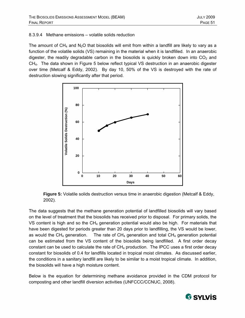
THE BIOSOLIDS EMISSIONS ASSESSMENT MODEL (BEAM) JULY 2009 FINAL REPORT PAGE 51 8.3.9.4 Methane emissions – volatile solids reduction
The amount of CH4 and N2O that biosolids will emit from within a landfill are likely to vary as a function of the volatile solids (VS) remaining in the material when it is landfilled. In an anaerobic digester, the readily degradable carbon in the biosolids is quickly broken down into CO2 and CH4. The data shown in Figure 5 below reflect typical VS destruction in an anaerobic digester over time (Metcalf & Eddy, 2002). By day 10, 50% of the VS is destroyed with the rate of destruction slowing significantly after that period.
0
20
40
60
80
100
0 10 20 30 40 50 6
Vola
tile
Solid
s D
estr
uctio
n (%
)
Days
0
Figure 5: Volatile solids destruction versus time in anaerobic digestion (Metcalf & Eddy, 2002).
The data suggests that the methane generation potential of landfilled biosolids will vary based on the level of treatment that the biosolids has received prior to disposal. For primary solids, the VS content is high and so the CH4 generation potential would also be high. For materials that have been digested for periods greater than 20 days prior to landfilling, the VS would be lower, as would the CH4 generation. The rate of CH4 generation and total CH4 generation potential can be estimated from the VS content of the biosolids being landfilled. A first order decay constant can be used to calculate the rate of CH4 production. The IPCC uses a first order decay constant for biosolids of 0.4 for landfills located in tropical moist climates. As discussed earlier, the conditions in a sanitary landfill are likely to be similar to a moist tropical climate. In addition, the biosolids will have a high moisture content.
Below is the equation for determining methane avoidance provided in the CDM protocol for composting and other landfill diversion activities (UNFCCC/CCNUC, 2008).

THE BIOSOLIDS EMISSIONS ASSESSMENT MODEL (BEAM) JULY 2009 FINAL REPORT PAGE 52
Equation 1.
Where:
= Methane emissions avoided during the year y from preventing waste disposal at the solid
waste disposal site (SWDS) during the period from the start of the project activity to the end
of the year y (tCO2e)
= Model correction factor to account for model uncertainties (0.9)
= Fraction of methane captured a the SWDS and flared, combusted or used in another
manner (zero for the first three years)
= Global Warming Potential (GWP) of methane, valid for the relevant commitment period (21)
= Oxidation factor (reflecting the amount of methane from SWDS that is oxidized in the soil or
other material covering the waste (0.10)
= Fraction of methane in the SWDS gas (volume fraction) (0.5)
= Fraction of degradable organic carbon (DOC) that can decompose (from Table 1)
= Methane correction factor (1)
= Amount of organic waste type j prevented from disposal in the SWDS in the year x (metric
tonnes) (monitored)
= Fraction of degradable organic carbon by weight in the waste type j (from Table 1)
= Decay rate for the waste type j (from Table 1)
j = Waste type category (index)
x = Year during the crediting period: x runs from the first year of the first crediting period (x = 1)
to the year y for which avoided emissions are calculated (x = y)
y = Year for which methane emissions are calculated
In the case of landfill disposal of biosolids, the decay rate constant k is 0.4 and the VS content of the material is used for the degradable organic carbon (DOC) value. In this way, the CH4 generation rate from landfilled biosolids can be determined.
Using Equation 1 and assuming a CH4 content of landfill gas of 50% (USEPA, 1997; USEPA 2005(b)) and a time of three years, one dry Mg of biosolids, assuming a solids content of 18%, will produce 0.067 Mg of CH4.

THE BIOSOLIDS EMISSIONS ASSESSMENT MODEL (BEAM) JULY 2009 FINAL REPORT PAGE 53 8.3.9.5 Methane emissions – Landfill gas capture
The IPCC provides a default value of 40-50% for landfill gas capture efficiency. The USEPA value for gas capture efficiency as detailed in the Waste Reduction Model (WARM) is 75%. Landfill-specific practices, such as time between waste deposition and gas collection implementation are important in determining the most appropriate value.
Once placed in a landfill, biosolids will become anaerobic within a period of weeks or months, and methane generation will commence. USEPA (2005(b)) notes that, in general, landfill gas production rates from mixed municipal solid waste peak “during the first or second year following waste placement and decline thereafter.” In the United States, most large municipal solid waste landfills (i.e. >2.3 million Mg) have landfill gas collection and control systems in place (Thorneloe, 2008). For such large landfills, federal regulations require installation of such systems within 5 years after waste burial. For smaller and older landfills, there are no landfill gas control requirements. It is likely that most biosolids will have decomposed considerably – emitting methane – before gas collection commences.
The only way to rigorously quantify methane collection efficiency is to have a measure of collected methane and fugitive methane emissions from the same area at the same time. While measures of collected methane are readily available, measures of fugitive emissions are considerably more difficult to obtain and have only been reported for a few landfills. Spokas et al. (2006) summarized intensive field studies of the methane mass balance for nine individual landfill cells at three French landfills with well-defined waste inputs. The collection efficiency was calculated as the ratio of recovered gas to empirically modeled gas generation. Specifically, Spokas et al. used the following equation:
Equation 2.
CH4 generated = CH4 emitted + CH4 oxidized + CH4 recovered + CH4 migrated + D CH4 storage
Methane generation was estimated using a gas production model. Emitted methane was measured by using either static chambers or an atmospheric tracer technique. Methane oxidation was measured by using a stable isotope technique that provides a conservative estimate of oxidation. Estimates of recovered methane were based on direct measurements at each landfill, and methane migration was based on calculations of methane diffusion through liners. Maximum potential methane storage was calculated from an estimate of waste porosity and changes in methane concentration and used as an upper limit of the value required to close a mass balance.
The results are summarized in Table 8. As illustrated, collection efficiencies for final clay covers were uniformly above 90% while the collection efficiency for the temporary covers was slightly above 50% in the summer and over 90% in the winter. Collection efficiencies were then recalculated to be consistent with other literature, which exclude the oxidation and migration

THE BIOSOLIDS EMISSIONS ASSESSMENT MODEL (BEAM) JULY 2009 FINAL REPORT PAGE 54 terms that can introduce more uncertainty. The differences are minor in consideration of the uncertainty of these types of studies.

THE BIOSOLIDS EMISSIONS ASSESSMENT MODEL (BEAM) JULY 2009 FINAL REPORT PAGE 55
Table 8: Collection efficiency for various cover reported in Spokas et al. (2006).
Cover Type Collection Efficiency
(%)a
Collection Efficiency
(%)b
Final clay cover (1 meter) with LFG recovery 91.5 92.6 Final geosynthetic clay with LFG recovery 51.5 53.0 Final clay cover (1 meter) with LFG recovery - summer 90.7 92.9 Final clay cover (1 meter) with LFG recovery - winter 97.8 98.6 Thin clay temporary cover (30 cm) with LFG recovery – summer 53.9 54.7 Thin clay temporary cover (30 cm) with LFG recovery – winter 93.2 95.1 Final clay cover (1 meter) with LFG recovery 99.2 100 Final geomembrane with horizontal gas collection 98.1 99.2
a Calculated as methane collected/(methane collected + emissions + oxidation + migration). b Calculated as methane collected/(methane collected + emissions).
Borjesson et al. (2007) reported on methane oxidation and collection at six Swedish landfills using Fourier-transformed infrared (FTIR) in combination with a tracer. While the emphasis of their study was on methane oxidation, sufficient data were published to calculate collection efficiency as in Equation 2 above. Data from two of the landfills (Hagby and Visby) were excluded from this review because it was reported that the gas collection systems were not working properly during the test period. The results for each landfill test are presented in Table 9. All landfills were active and only minimal information was reported on the cover type. These data are likely applicable for daily covers in the context of U.S. landfills, although U.S. landfills do not typically use sludge as a cover material.
Table 9: Collection Efficiency for Various Covers Reported in Borjesson et al. (2007)
Cover Type Collection Efficiency
(%)a
Fiborna (wood chips and sludge) 68.4 Fiborna (wood chips and sludge) 65.0 Fiborna (wood chips and sludge) 70.0 Heljestorp (sewage sludge and soil) 57.8 Hogbytorp (sewage sludge and soil) 33.9 Hogbytorp (sewage sludge and soil) 43.2 Sundsvall (sewage sludge and soil) 63.3
a Calculated as methane collected/(methane collected + emissions).
Mosher et al., (1999) reported a summary of methane emissions from nine landfills in the northeastern US. Emissions were measured by both static chambers and a tracer flux technique. Two of the landfills collected gas, making it possible to compare emissions to gas amount of gas collected. One of the two landfills was closed and had a geomembrane plus soil cover. A collection efficiency of 90.5% was calculated. However, the authors indicate that the

THE BIOSOLIDS EMISSIONS ASSESSMENT MODEL (BEAM) JULY 2009 FINAL REPORT PAGE 56 gas collected was not measured accurately, which casts some doubt on this value. This collection efficiency is nonetheless likely to be reasonable from two perspectives. First, this landfill had the lowest emissions of the sites studied, and second, the collection efficiency is consistent with other values in this review. A collection efficiency of 70% was calculated for an active landfill in which part of the landfill was covered with a geomembrane but other had daily cover only.
Huitric and Kong (2006) reported collection efficiencies for the Palos Verdes Landfill (PVLF) in Los Angeles County. The PVLF was closed in 1980, has a 5-foot thick clay cap and an active gas collection system. The efficiency of the LFG collection system at the PVLF was calculated to be 94 to 96%. While these results are consistent with Spokas et al. (2006), methane generation at the PVLF is relatively low given the refuse age. Total gas collection was equivalent to 36.3 gm CH4 (m-2 d-1). In Huitric et al (2007), the collection efficiency determined was supported by the results of a static flux chamber study completed at the PVLF. In fact, even higher collection efficiencies were reported for the PVLF.
Lohila et al. (2007) reported methane fluxes for a section of a Finnish landfill that included an active disposal area and a sloped area. The active area was covered daily with soil and construction and demolition waste rejects, and the sloped area had a cover that included 0.2 to 0.5 meters of compost over 0.5 to 2 meters of diamicton and clay. Three estimates of collection efficiency were reported. First, it was reported that the mean methane flux over seven days was reduced by 79% when the gas collection system was turned on. This measurement was made by using methane concentration data coupled to an eddy covariance method. A second measure of methane flux with the gas system activated suggested a reduction of only 39%. However, this second estimate was based on 7 to 10 static chamber measurements and is not likely representative of the entire landfill. The third estimate was made by comparing the mean methane emission to the volume of gas collected and assuming that methane production was the sum of emissions plus collection. This resulted in an estimate of 69% collection efficiency.
In 2008, the USEPA updated its methodology for estimating emissions from municipal solid waste landfills. Updated emissions factors for inclusion in the AP-42 Section 2.4 landfill management standards were developed from recent research. This recent work includes estimates of landfill gas capture efficiency, including the key variable of time between deposition of waste and installation of gas collection systems.
A typical landfill will not capture gas from the most recent two to five years of waste. The impact of excluding the most recent portions of the waste mass from the collection system is magnified by the fact that the LFG emission rate is greatest in the first few years after placement and drops rapidly with time. Therefore, a system capable of collecting 90% of the gas generated from the landfill cells in which it is installed is operating at reduced landfill-wide collection efficiency (i.e., less than 90%) due to the loss of gas from cells that have yet to be capped and connected to the collection system. All active landfills contain open cells and waste cells that have yet to be capped and fitted with a gas collection system. Table 10 demonstrates the

THE BIOSOLIDS EMISSIONS ASSESSMENT MODEL (BEAM) JULY 2009 FINAL REPORT PAGE 57 impact of the delay in collecting gas from newer cells. The values in this table were generated using the first order decay model (Pelt, 1993) and assuming a Lo of 100 and a k of 0.04. The landfill was assumed to be operating (i.e. accepting waste) over a 20 year timeframe.
Table 10: Impact of delays in collecting gas from newer landfill cells.
Effective Landfill-wide Gas Collection Efficiency Time Between Waste Placement and Initial
Gas Collection for Individual Cells
(years) System Collection Efficiency 90%
System Collection Efficiency 85%
1 84 79 2 77 73 3 72 68 4 66 62
5 60 57
6 55 52
Thus, if it is assumed that gas collection becomes effective in 3 years, a reasonable assumed rate of gas capture is 70%.
8.3.9.6 Methane emissions – using biosolids as cover material
It is likely that, for biosolids-generated CH4, collection efficiency will be low, whether the biosolids are mixed into solid waste or used as daily cover. If they are used for final cover (i.e. not mixed to create a ‘soil’), no provision for gas collection would be used and so a higher rate of CH4 release would be likely. On the other hand, a biosolids-based cover material that is properly composted and managed as an aerated final cover soil on a landfill would not emit methane; on the contrary, it will mitigate methane emissions from the landfill below it through methane oxidation (Huber-Humer, 2008).
8.3.9.7 Nitrous oxide emissions
There have been few studies on emissions of N2O from landfilled biosolids or biosolids used as landfill cover. The IPCC guidance document on waste mentions landfills as a source of N2O, but does not provide specific guidance on sources of N2O within the landfill or means to quantify N2O release (Pipatti et al., 2006). One study measured N2O emissions from landfills in Sweden, where soil or biosolids were used as cover soil (Börjesson and Svensson, 1997). On two of the four landfills included in the study, biosolids was used as soil at a depth of 0.5-1 m. Nitrous oxide emissions from the biosolids cover soil sites ranged from -0.011 to 35.7 mg N2O-

THE BIOSOLIDS EMISSIONS ASSESSMENT MODEL (BEAM) JULY 2009 FINAL REPORT PAGE 58 N / m2 / h. For comparison, N2O emissions from sites covered with soil ranged from -0.0017 to 1.07 mg N2O-N / m2 / h.
These results suggest that use of biosolids as landfill cover can be expected to release N2O. It is likely that landfilled biosolids would release N2O at the same or a similar rate to materials used as surface cover, as the environment within a landfill will be more oxygen deficient than the environment at the landfill surface.
In addition, biosolids contain sufficient moisture and high nitrogen. This suggests that for other components of MSW that may be moisture and N limited, mixing with biosolids will increase the potential for N2O formation. Limited studies have suggested that this can occur for methane, and similar results would be expected for N2O (Chan et al., 2002).
8.3.10 Combustion
There is a growing interest in combustion of biosolids as a management option that includes provisions for energy capture. Approximately 50% of the biosolids produced in Québec is incinerated, including in Montréal, Longueuil, Québec and Laval). Pyrolysis, combustion under high pressure and temperature with limited oxygen, or modifications of this process are receiving attention as potential alternatives to standard combustion technologies. As there are no operating facilities at this time, actual efficiencies or even the efficacy of these technologies for biosolids combustion is not known. A single facility that was operating in Perth, Australia, was shut down due to operational difficulties. As a result, for this project emissions factors for combustion of biosolids are based only on proven technologies currently in use. The most prevalent technologies for biosolids combustion are multiple hearth furnaces and fluidized bed combustion facilities. These are common technologies for co-combustion, as well as mono-incineration of biosolids (Werth and Ogada, 1999).
8.3.10.1 Carbon dioxide emissions from incineration of biosolids
Mono-incineration of biosolids requires supplemental energy from the combustion of natural gas or fuel oil, especially if the total solids content of the biosolids is <65%. Biosolids dewatered using conventional dewatering technologies (e.g. centrifuges, rotary presses, belt filter presses, etc.) generally achieve total solids contents of 20-30 % total solids. Although City X did not include their total solids content for their dewatered cake, they use rotary presses for dewatering, so it can be assumed that the total solids content of their cake is much less than 65%. Energy requirements for dewatering technologies are discussed in another section of this report. For combustion, a default value of no additional energy required has been included – which is reasonable for a modern, well-managed fluidized bed incinerator. However, included in the possible data inputs, is the option to enter external energy required for combustion, such as natural gas or fuel oil. Even with drier biosolids, bringing the incinerator to operating temperature requires supplemental fuel, and the fuel required for afterburners in multiple hearth incinerators can be 85-90% of the total system fuel requirements.

THE BIOSOLIDS EMISSIONS ASSESSMENT MODEL (BEAM) JULY 2009 FINAL REPORT PAGE 59 At the Northeast Ohio Regional Sewer District (Cleveland, OH) approximately 34,500 dry Mg of biosolids are combusted annually in multiple hearth furnaces (B. Dominak, pers. comm.). Most of the solids are dewatered with the Zimpro process to approximately 47% dry matter; the remainder is processed in centrifuges that produce a cake with approximately 31.5% solids. A total of approximately 4.56 million m3 of natural gas are used to burn the solids, resulting in an average of 132 m3 of natural gas use per Mg of solids burned. These fuel requirements are expected to be reduced by 95% with the installation of new fluidized bed incinerators that include comprehensive energy recovery.
The power required for the operations of the Westerly incinerators is approximately 186 kW (250 hp). With two of them running (not simultaneously) for a combined total of 7,000 hours each year, the result is 285 kWh of energy use per Mg wastewater solids processed. It is estimated that the power required for operations of new fluidized bed incinerators (i.e. that include comprehensive energy recovery) will be 70% of the existing power requirements for the multiple hearth units, or about 200 kWh / Mg solids burned. Less energy is required to operate a fluidized bed incinerator because and afterburner is not required to treat volatile organic compounds. Operational electricity requirements include blowers, feed mechanisms, and air emissions control systems.
The Northeast Ohio Regional Sewer District (Cleveland, OH) has four multiple hearth incinerators at its Southerly WWTP and two at its Westerly WWTP. The wastewater solids at Southerly are thermally conditioned and dewatered with high solids centrifuges that produce a cake containing approximately 47% dry matter. Westerly's wastewater solids are chemically conditioned and dewatered with high solids centrifuges that produce a cake with approximately 31.5% solids.
During 2007, a total of 2.8 million m3 (99,000 mcf) of natural gas were used to burn ~30,020 dry Mg (70,400 wet U.S. tons) of biosolids. In addition, a total of 1.756 million m3 (62,000 mcf) of natural gas was used to burn 4,570 dry Mg (16,000 wet U.S. tons) of biosolids. These result in natural gas use figures of 93 m3 / Mg dry biosolids processed and 384 m3 / Mg dry biosolids processed, respectively. The difference in fuel use is due to the difference in moisture content of the biosolids.
The fuel requirements at Southerly are expected to be reduced by 95% with the installation of new fluidized bed incinerators that include comprehensive heat recovery and the generation of electricity. This would require natural gas at the rate of 5 m3 / Mg biosolids processed. The new incinerators are scheduled to be placed into service in 2012.
The power required for the operations of Cleveland's incinerators is about 190 kW / h for each of the six multiple hearth units. This includes the incinerators and air emissions control systems. The Southerly facilities processed approximately 30,020 Mg biosolids in 18,700 hours of run time in 2007, resulting in a rate of about 118 kWh / Mg of dry biosolids processed. The Westerly facilities, running approximately 7,000 total hours, used approximately 291 kWh / Mg

THE BIOSOLIDS EMISSIONS ASSESSMENT MODEL (BEAM) JULY 2009 FINAL REPORT PAGE 60 biosolids processed. This facility manages biosolids with a higher moisture content. It is estimated that the power required for operations of new fluidized bed incinerators will be slightly less. However, each of the new fluidized bed incineration systems will be equipped with boilers that will utilize the heat in each incinerator’s exhaust gases to produce high pressure steam. The steam will be used operate a turbine that will produce electricity that will be used to operated fluidizing air blowers and other equipment in the incineration facility.
8.3.10.2 Methane emissions from incineration
For incinerators that operate fairly continuously, emissions of CH4 are minimal. The IPCC provides a default value of 4.85 x 10⁻⁵ kg CH4 emitted / dry kg wastewater solids burned. This is small enough in comparison to other emissions associated with incineration to be considered negligible.
8.3.10.3 Nitrous oxide emissions from incineration
Nitrous oxide emissions from biosolids combustion vary primarily as a function of the combustion temperature. The current best available technology is the fluidized bed incinerator; these are being installed whenever wastewater solids incinerator upgrades are completed.
Multiple hearth furnaces have long been used for mono-incineration of biosolids. In these facilities, temperatures vary based on the location in the furnace, suggesting a greater potential for N2O emissions than from fluidized bed incinerators, where temperature is more uniform (Werther and Ogada, 1999).
The IPCC provides default values for N2O release from biosolids combustion (Sabin et al., 2006). These are based on data provided for combustion of different types of biosolids and are summarized in Table 11. The factors are 900 g of N2O per wet (10% solids) Mg biosolids combusted and 990 g of N2O per dry Mg biosolids combusted. This is equivalent to 800-1500 g-N2O / Mg dry sludge. The data that formed the basis for these default values were based on single point observations at combustion facilities (Gutierrez et al., 2006; Svoboda et al., 2006).
Suzuki et al. (2003) conducted a study to refine N2O emission factors from biosolids incinerators. Continuous monitoring of N2O and freeboard temperature was conducted at six facilities between 7-14 days. The data showed high N2O concentrations, ranging from 100-300 ppm (approximately 300-900 times the ambient N2O concentration) and it was observed that N2O emissions decreased with increasing freeboard temperature. Large fluctuations in N2O concentrations measured over the course of the study indicate that emission factors based on short-term analysis or grab sampling are not likely accurate.
Nitrous oxide emission factors of 1,520-6,400 g N2O / dry tonne biosolids were calculated. These emission factors were higher than the emission factors previously used to calculate N2O emissions in Japanese incinerators; however, the previous numbers were based on short-term

THE BIOSOLIDS EMISSIONS ASSESSMENT MODEL (BEAM) JULY 2009 FINAL REPORT PAGE 61 analysis and grab sampling and were therefore considered unreliable. Furthermore, this emission factor range is higher than the values of 800-1,500 g N2O / dry tonne published in the “Good Practices Guidance and Uncertainty Management in National Greenhouse Gas Inventories” published by the IPCC. However the data that formed the basis for these default values were also based on single point observations at combustion facilities (Gutierrez et al., 2006; Svoboda et al., 2006) and may not be as reliable as those derived by Suzuki et al. (2003).
Comparing the N2O emission results to freeboard temperature and assuming a linear relationship yielded the following equation:
η = 161.3-0.140Tf
Where η is the % of total N that is volatilized as N2O and Tf is the average highest freeboard temperatures from the fluidized bed facilities. This equation can be used to estimate the N2O emission factor of a given incinerator from its long-term average freeboard temperature.
Based on the rigor with which the Suzuki et al. (2003) was conducted, and concerns regarding the reliability of emission factors based on much shorter analysis times, the calculations in the BEAM are based on the findings of the Suzuki et al. (2003) study.
In other studies, the relative amounts of N2O produced ranged from 200 pg (N2O, dry basis) / mg m3) for dry biosolids, 325 for semi-dry biosolids, and 600 for wet biosolids. These relative emissions are not provided for in terms of Mg of biosolids. Svoboda et al. (2006) also argue that increased oxygen content in the combustion chamber will also increase N2O concentration, however, the data shown clearly does not follow this pattern (Suzuki et al., 2003). Co-combustion of biosolids with coal also creates high N2O emissions. From the data given in Svoboda et al (2006), it is not clear that co-combustion of coal and biosolids or MSW and biosolids should be treated differently from mono-combustion of biosolids with respect to net emissions. For this study, mono and co-combustion are treated in the same manner.
Table 11: Rates of N2O emissions from different types of combusted biosolids.
Country Biosolids g N2O/Mg Biosolids Weight basis
Dehydrated 900 Wet weight
Lime sludge 294 Wet weight Japan
Cake 1520 - 6400 Dry weight
Germany Cake 990 Dry weight
Montreal (preliminary data, 2008) Cake 1 – 5 kg Dry weight
IPCC default - 990 Dry weight

THE BIOSOLIDS EMISSIONS ASSESSMENT MODEL (BEAM) JULY 2009 FINAL REPORT PAGE 62
IPCC default - 900 Wet weight
Additional studies have provided more detail on these emission factors. Sänger et al., (2001) tested the importance of total solids content on N2O emissions from lab-scale fluidized combustion in a semi-pilot-scale facility. Emissions were similar for wet (20-40% solids), semi-dry (30-55% solids), and dry (> 80% solids) biosolids. No decreases were observed for N2O emissions with staged combustion, although increasing the freeboard temperature to > 900˚C reduced N2O emissions. Another study notes that for co-combustion of biosolids with coal and wood in a fluidized bed, only a low percentage of the fuel nitrogen is converted to N2O (Leckner et al., 2004). No specific data is given on actual N release from these systems.
As part of the evaluation of combustion, discussions were held with facility operators in the US and Canada. North East Ohio recently conducted a greenhouse gas analysis as part of a plan to upgrade from multiple hearth to fluidized bed incinerators. The N2O emissions they independently calculated from their current system are roughly predicted by the Suzuki et al. equation provided above. The same is true for preliminary measurements using FTIR technology of N2O emissions from the four Montréal incinerators, which are also multiple hearth units running at approximately 760o C. Montréal expects to have long-term continuous FTIR monitoring in place by mid-2009.
There is widespread agreement that additional, continuous monitoring of N2O emissions are needed.
Other factors with smaller influences on N2O emissions from combustion of biosolids include the following:
• The number of start-ups and shut-downs required for maintenance: Generally, modern fluidized bed incinerators are shut down only a couple of times a year (Metcalf & Eddy, 2003; B. Dominak, pers. communications). However, the Québec City incinerator has greater than 40 shutdowns annually. Multiple hearth furnaces are shut down more often – 4 to 5 times each year. Each of these cycles requires supplemental fuel (natural gas) to return the furnace to high temperature. However, N2O emissions will not necessarily increase dramatically during start-up, because wastewater solids will not be injected until the high combustion temperature is reached. However, sometimes an incinerator that is not in use is kept on standby, burning fuel, in order to be ready to process solids on short notice.
• Emissions reduction technology can also be a source of N2O emissions depending on the processes used. Use of selective non-catalytic reduction (SNCR) using urea as a catalyst can be a significant source of additional N2O. Use of SCR or SNCR with ammonia is a much less

THE BIOSOLIDS EMISSIONS ASSESSMENT MODEL (BEAM) JULY 2009 FINAL REPORT PAGE 63
significant source of N2O, however no details on emissions increase with urea based SNCR are provided.
• The Northeast Ohio Regional Sewer District (2008) included in its debit accounting the small amounts of fossil fuel-derived substances in biosolids combusted in an incinerator (i.e. traces of oils, fuels, etc.). As biosolids generally contain minimal concentrations of these constituents and, if present, would be converted to CO2, they are unlikely to have much significance in comparison to N2O and CH4 emissions, would likely create equivalent emissions from one biosolids management scenario to another, and are likely best ignored.
Regarding combustion of wastewater solids, there is one final aspect of note, use of ash in agriculture or cement or brick manufacturing. Depending on the quality of the wastewater solids and the resulting ash, this material is sometimes used as a replacement for agricultural lime and to provide micro-nutrients (i.e. trace elements). Alternatively, ash is used in place of some portion of the lime needed for manufacturing cement or, less commonly, brick. This is the case in City X, where approximately eight tonnes per day of ash from their fluidized bed incinerator are transferred to a cement kiln where it is incorporated into the cement. Conversely, Laval transfers thermally dried biosolids (95% total solids) to a cement kiln where they are incinerated as a fuel source in the kiln. In any case, these uses of ash will displace some use of lime (CaCO3). Given the significant GHG emissions associated with lime production (see section on alkaline stabilization, above), ash use can provide a credit to the biosolids management program.
8.3.11 Land application
Land application of biosolids and biosolids compost is commonly practiced in Canadian jurisdictions, and represents an important utilization option for biosolids nationwide. Several of the participating jurisdictions engage in some form of biosolids land application. The Regional District of Nanaimo, applies biosolids in a forest fertilization project; Metro Vancouver biosolids are applied to disturbed lands including mineral and aggregate mines; the Region of Halton applies liquid and dewatered biosolids to agricultural land; and Moncton blend their biosolids compost with topsoil to provide biosolids based products for multiple uses. As with other unit processes, there are GHG debits associated with biosolids land application. These sources are described below.
8.3.11.1 Carbon dioxide emissions from land application
As noted above, fuel and electricity consumption are the sources of anthropogenic CO2 emissions from biosolids management programs. For land application, fuel is burned by transporting biosolids to farm fields and other end-use sites and during the land application
THE BIOSOLIDS EMISSIONS ASSESSMENT MODEL (BEAM) JULY 2009 FINAL REPORT PAGE 64 process (e.g. using tractors and spreaders). Discussion of these CO2 emissions appears at the beginning of the literature review section.
8.3.11.2 Methane emissions from land application
When biosolids are land applied in accordance with provincial regulations and / or guidance, they are generally applied in small, dispersed amounts to aerobic soils. Thus, land applied biosolids are not likely a significant source of methane emission. Biosolids are not typically applied to anaerobic soils due to concerns regarding nutrient leaching and run-off. Because of this, CH4 release from land application of biosolids is considered negligible. Previous work has shown minimal release even in poorly drained soils (Ball et al., 2004; Jones et al., 2006). For example, in a three year study, CH4 emissions from a poorly drained soil in Scotland ranged from 0.3 to 0.5 kg CH4-C / ha with an annual biosolids application that provided approximately 3,000 kg total N / ha (Jones et al., 2006).
However, if biosolids are stored onsite in piles prior to being land applied, anaerobic conditions are likely (Peckenham et al., 2008) and methane generation could occur. One study documented release of CH4 from stored raw and digested manure with higher releases during summer months and from raw materials (Clemens et al., 2006). This suggests that storage of wet material should be minimized during summer months. Conversely, stored biosolids with low moisture content (e.g. pellets), compost, and alkaline biosolids are not likely to emit significant quantities of GHGs until they are land applied and carbon mineralization occurs.
8.3.11.3 Nitrous oxide emissions - agronomic rates
Biosolids are generally applied to agricultural land as a substitute for synthetic fertilizers. By regulation, they are applied at agronomic rates. The agronomic rate is the amount of biosolids required to provide the amount of nutrients needed by the crop being grown. In most cases, nitrogen is the plant nutrient by which the agronomic rate is set; however, in Québec, phosphorus is the limiting factor. Canadian provincial regulations and guidelines for biosolids land application specify use of agronomic rates or include agronomic rate requirements in case-by-case permits. Refer to Table 12 for a summary of provincial requirements. Limiting biosolids applications to the agronomic rate has important implications. Not only does it limit the total amounts of trace elements of concern (e.g. heavy metals) applied, it also limits the total nitrogen (N), which reduces the potential for N2O emissions.
A number of studies have quantified N2O release from soil. Refer to Table 13 for a summary. The IPCC gives direct and indirect default emissions factors for N2O emissions for fertilizer use. Direct emissions from application of synthetic fertilizer, compost, or municipal biosolids are estimated to generate N2O from 1% of the total N added. A higher emissions factor is used for cattle, pig, and chicken manures (2%). Grant et al.,(2006) provide default factors for N2O emissions from fertilized soils of 1.25 ± 1% of total N applied. Development of country specific emissions factors are encouraged by the IPCC for more precise estimates. The IPCC also

THE BIOSOLIDS EMISSIONS ASSESSMENT MODEL (BEAM) JULY 2009 FINAL REPORT PAGE 65 encourages use of manures as a means to reduce N2O emissions from agricultural soil (Metz et al., 2001).
A study of the total GHG emissions using the DAYCENT model, a process-based biogeochemical model used by scientists to estimate N2O emissions, in combination with data from several counties in the northern US, determined that soil N2O emissions accounted for 31-59% (88-284 g CO2 / kg dry grain) of the total GHG emissions from corn production (Kim and Dale, 2008).
8.3.11.4 Nitrous oxide emissions – climate and soil
A number of studies have documented soil and climate specific factors that control N2O emissions (Fine et al., 1998; Grant et al., 2006; Peterson, 1999;Rochette et al., 2008). Fine et al. (1989) conducted a greenhouse study measuring N2O release from two soils that had been amended with two different rates of activated sludge. Nitrous oxide emissions were detected only after NO3
- concentrations had increased and were significant only in the high clay content soil. In a study conducted on a well-drained soil in Denmark, Peterson et al. (2004) observed N2O release across different fertilizer and manure treatments of 0.14-0.64% of total N added, which is below the default IPCC value. Grant et al. (2006) measured N2O flux from two soils in Canada to determine if cooler and dryer conditions would reduce N2O emissions. The site in Alberta, which was cooler and dryer, had significantly lower emissions than the site in Ontario. Rochette et al. (2008) tested N2O emissions from a site south of Québec City. Emissions in the clay soil ranged from 12-45 kg N2O / ha over the three year period of the study. Emissions in the loam soil ranged from 1.0-1.1 kg N2O / ha over the same period. In general, if anoxic conditions are not present (i.e. soil is very well drained or coarse), even if a product has a high potential to emit N2O, it is unlikely to cause emissions (Chantigny, pers. comm.). On a poorly drained grassland site in Scotland, emissions from soils that had received high loading rates of biosolids (3,066 kg N / ha) were 4.3 ± .5% of total N in year 1 and 1.3 ± .2% of total N in year two with rainfall of 1,107 mm and 718 mm in years 1 and 2, respectively (Jones et al., 2007). Emissions tend to be significantly greater in warmer months, however, emissions have also been measured from soils over the winter (Dobbie and Smith, 2001; Jones et al., 2007).
In a field study in Scotland, emissions were highest during the three summer months following amendment addition in June (Jones et al., 2007). Emissions increased after rainfall events and were also detected in the winter following heavy rains. Peterson (1999) observed the highest N2O fluxes in fertilizer and manure amended soils in the spring when soils were saturated and crop growth was slow. Rochette et al. (2000) observed a flux of N2O in a field study after manure addition in June which was followed by a heavy rain event. Ball et al. (2004) also noted fluxes after rainfall events. In this study a range of biosolids products were compared to synthetic N and cattle slurry. Nitrous oxide release continued over a longer period in organic amended soils but total emissions were lower than those from plots that received synthetic fertilizer. These results suggest that N2O fluxes are highest as the organic N in manures or

TF
HE BIOSOLIDS EMISSIONS ASSESSMENT MODEL (BEAM) JULY 2009 INAL REPORT PAGE 66
biosolids is mineralized and becomes available over time from denitrification in anaerobic soil microsites or after high rainfall when soil moisture is high.
In summary, poor drainage and fine soil texture are the primary factors that contribute to elevated N2O release. Site-specific factors, including the percentage of time that soil moisture is greater than 60%, the clay content of the soil, and the relative position of a field (e.g., low lying areas) will determine the extent of N2O release (Grant et al., 2006). The research findings suggest that because denitrification occurs under anoxic or anaerobic conditions, restricting applications to coarser textured soils would reduce the potential for N2O emissions. Wet conditions will tend to increase N2O emissions.

HE BIOSOLIDS EMISSIONS ASSESSMENT MODEL (BEAM) JULY 2009 INAL REPORT PAGE 67
Province Regulatory Maximum Agronomic Rate Notes
Alberta Maximum of 25 dt/ha every 3 yrs. Factors that are considered in determining application rates include
nitrogen and phosphorus concentrations in the biosolids, soil texture, soil slope, and depth to potable aquifers.
British Columbia
Varies, case-by-case, based on crop nutrient needs and avoiding nutrients moving off-site; rates as high as 300 dt/ha for a one-time reclamation of disturbed lands.
Application rate is specified by the applicant and approved by the Ministry of Environment.
Manitoba Addressed on a case-by-case basis under the province’s environmental protection act.
New Brunswick Maximum of 8 dt/ha every 3 yrs., but based on crop nutrient needs; biosolids must meet highest quality metals standards.
Covered in “Guidelines for Issuing Certificates of Approval for the Utilization of Wastes as Soil Additives”
Newfoundland Probably addressed on a case-by-case basis under the province’s environmental protection act.
Nova Scotia Based on required nutrient management plan that considers crop nutrient needs and properties of the biosolids.
Application rates are determined using a methodology outlined in “Guidelines For Land Application and Storage of Biosolids in Nova Scotia," (2004) involving nutrient management planning.
Ontario Based on crop nutrient needs and site constraints, to a maximum of 22 dt/ha every five years.
If biosolids meet the strictest trace element concentration standards, they me be applied to the maximum rate. Otherwise, if they meet the less strict trace element concentration standards, they may be applied only up to 8 dt/ha every five years.
Prince Edward Island
Probably addressed on a case-by-case basis under the province’s environmental protection act.
Québec Application rates are limited based on agronomic phosphorus requirements.
Agricultural guidelines: http://www.mddep.gouv.qc.ca/matieres/mat_res-en/fertilisantes/critere/index.htm Silvicultural and degraded site applications have different limits.
Saskatchewan Based on crop nutrient needs and existing N in soil; typical maximum rate is ~30 dt/ha/yr.
Covered by “Land Application of Municipal Sewage Sludge Guidelines EPB 296”
Table 12: Land application of agronomic rate limits or guidance by province.
TF

THE BIOSOLIDS EMISSIONS ASSESSMENT MODEL (BEAM) JULY 2009 FINAL REPORT PAGE 68
8.3.11.5 Nitrous oxide emissions - higher rates of land application
Nitrous oxide emissions have also been shown to increase when application rates are in excess of agronomic requirements. Rochette et al. (2000) monitored N2O emissions from a soil in Québec that had received synthetic fertilizer (150 kg N) and pig slurry at two rates (60 and 120 Mg / ha). Nitrous oxide emissions for the high rate of slurry application were 1.65% of N added and decreased to 1.23% of N added for the lower rate of slurry application. In comparison, the synthetic fertilizer application resulted in emissions of N2O of 0.62% of N added. The authors suggest that these values correspond with the IPCC default value of 1.25 that was the default at the time that this study was published. Since that time, however, the IPCC default values have been reduced and separate values have been suggested for different types of animal manures including pig slurry. Other studies have shown increased emissions based on over-application of N (see below). Kim and Dale (2008) calculated N fertilization rates to provide sufficient N for plant growth while simultaneously limiting the potential for N2O evolution. Using the DAYCENT model, excess addition of fertilizer resulted in significant increases in N2O fluxes from soils.
Other studies have shown variable results in terms of N2O emissions at high agronomic / reclamation rates. A lab incubation tested the addition of 10% dry weight of a range of biosolids to a single soil (Stucyznski and McCarty, 2007). Soils were maintained at field capacity in the dark for the incubation. Average N2O release was 0.021% of total N applied. In field studies in Scotland, application of high rates of biosolids on a poorly drained soil resulted in relatively low N2O emissions in one study and very high emissions in another (Scott et al., 2000; Jones et al., 2007). In the first study, biosolids were applied at 185 Mg / ha for 3 years (total N / year was 2,500 kg / ha) (Scott et al., 2000). Nitrous oxide emissions were up to 1% of total N applied. In a follow-up study on similar soils, up to 5% of total N applied was emitted as N2O for biosolids added to soils with a total N addition of 3,066 kg / ha / yr. A study on tropical soils found increases in N2O as the rate of biosolids application increased to well above standard agronomic rates (Fernandes et al., 2005).
8.3.11.6 Timing of emissions from land application
Studies have also been undertaken to monitor N2O emissions over time. In a six-week lab incubation, 100 different animal manures were added to a soil (Calderon et al., 2004). Measurable N2O emissions occurred during the first three weeks of the incubation. The authors tested denitrification enzyme activity, NH4, and other variables and determined that there was no correlation between any of these variables and N2O production. In another lab incubation of soils that had received high rates of biosolids composts, N2O emissions peaked in weeks 3-4 (Zarman et al., 2004). In this particular study, the plots from which the soils were collected had received a split application of biosolids compost, either composted with rice hulls or sawdust, since 1978, applied at a rate of 240 kg N / ha. The rice hull compost had a carbon-to-nitrogen (C:N) ratio of 14 and the sawdust compost had a C:N ratio of 20.

THE BIOSOLIDS EMISSIONS ASSESSMENT MODEL (BEAM) JULY 2009 FINAL REPORT PAGE 69 8.3.11.7 Nitrous oxide emissions - incorporation or topdressing
Rochette et al. (2006) found that, in course-textured soil, having the biosolids topdressed or incorporated does not make a significant difference in N2O emissions. However, when applied to fine-textured soil, significantly higher N2O emissions occurred when the biosolids were not incorporated (3.3% of N) in comparison to when the biosolids were tilled in (1.3%).
8.3.11.8 Nitrous oxide emissions – biosolids type
There are characteristics of different amendments that will influence the potential for N2O release. As N2O is formed as a half reaction in the oxidation of carbon by anaerobic soil microbes, a readily available carbon source is necessary for this reaction to occur (Wan et al., 2009; Chantigny, pers. comm.). Carbon in anaerobically or composted biosolids may be less available for microbial decomposition than carbon in animal manures or primary solids (Ball et al., 2004; Peterson, 1999). However, if soil N is limiting, then the addition of N even in a stable compost may still trigger increased N2O emissions (Chantigny, pers. comm.). In addition, the form of N in the amendment may increase the potential for N2O emissions (Perron and Hébert, 2004). If N is present primarily as organic N, it must be converted to mineral N before there is a potential for N2O production during denitrification reactions. If a substantial portion of N in the amendment is present in mineral form, this will increase the available N for denitrification and N2O production. The IPCC sets higher default emissions factors for animal manures (e.g. pig slurry, 2% total N) than for municipal biosolids and synthetic fertilizers (1% total N), because of the combination of available carbon and high mineral N content in the former.
Peterson et al. (2004) measured emissions from spring barley grown in Denmark in a well-drained soil (77% sand) that had been fertilized with a) raw manure, b) anaerobically-digested manure, and c) synthetic fertilizer. Nitrous oxide emissions from the anaerobically-digested material (food waste and manure) were similar to synthetic fertilizer and significantly lower than raw manure. This was attributed to lower and more stable carbon in the digested material.
In another study, emissions from digested liquid biosolids, pelletized biosolids, and biosolids composts were compared (Ball et al., 2004). The study also included raw cattle slurry. Emissions were highest from the cattle slurry (15.3 kg N / ha over a 3 year period), with lower emissions from all biosolids products (10.3 kg N / ha for compost – 8.0 kg N / ha for pellets). These results suggest that application of primary biosolids may result in higher N2O emissions than secondary, digested biosolids. As the volatile solids content of the biosolids is reduced, either through anaerobic digestion or composting, it is likely that the potential for N2O emissions will decrease. In addition, compost will have lower available N than biosolids, which will further decrease the potential for denitrification and formation of N2O (Huang et al., 2004).

TF
HE BIOSOLIDS EMISSIONS ASSESSMENT MODEL (BEAM) JULY 2009 INAL REPORT PAGE 70
8.3.11.9 Impact of C:N ratio on N2O emissions
Some literature suggests that increasing the C:N ratio of the amendment can decrease N2O release. In a greenhouse study, plant materials with C:N ratios ranging from 8:1 to 118:1 were added at low rates to a high clay content soil (Huang et al., 2004). Emissions were highest with application of the 8:1 material and lowest with application of the 118:1 material. In another lab incubation using high rates of biosolids addition, biosolids with a C:N ratio < 16:1 had higher emissions than those with a C:N ratio > 19:1 (Stuczynski and McCarty, 2007). This information is pertinent for reclamation sites where biosolids can be blended with high C residuals. It is also important for composted biosolids, as composting will result in a higher C:N ratio product, and, thus, lower N2O emissions.
8.3.11.10 Nitrous oxide emissions - storage
Research is limited regarding the potential emissions from storage or curing of biosolids. One study showed fairly consistent N2O emissions from stored manure regardless of time of year or whether the manure had previously been digested (Clemens et al., 2006). Findings from studies on animal manures have differed. High N2O releases (~30% of total N) have been measured from deep animal manure deposits in farmyards, where compaction is significant and urine and water accumulate (Chantigny, pers. comm.). However, another study of stored pig and cattle farmyard manures found N2O releases of 2.6% and 4.3% of the total-N, respectively (Thorman et al., 2007). While these latter emission rates are not significant, they are higher than the IPCC default value of 2% of total N. While biosolids, especially those that are stabilized, are likely to emit N2O at lower rates than animal manures (IPCC, 2007), further research is warranted to understand the potential impacts of storage of semi-solid biosolids at the wastewater treatment plant or in the field.

THE BIOSOLIDS EMISSIONS ASSESSMENT MODEL (BEAM) JULY 2009 FINAL REPORT PAGE 71
Table 13: Summary of research reporting N2O emissions from soils and treated soils.
Author Title Year Summary Comments
Kim and Dale Effects of nitrogen fertilizer application on GHG emissions and economics of corn production
2008 Use DAYCENT model to calculate when yield increases and resultant carbon are high enough to compensate for emissions associated with N application- determine an optimum fertilizer rate re GHG. Emissions for corn range from 227 to 518 g CO2/dry kg grain
N2O emissions from soil account from 31-59% of total GHG emissions from crop (88-284 g CO2/kg grain. N fertilizer associated with grain 63-97 g CO2e/kg grain or 17-28% total emissions
Rochette et al. Nitrous oxide emissions respond differently to no-till in a loam and a heavy clay soil 2008 High clay soils with high organic matter release significantly more N2O than coarser textured
soils under no till (Canadian study) In clay soil, NT doubled N2O emissions in comparison to plow. In loam soil emissions were similar under NT and plow
Jones et al. Influence of organic and mineral N fertilizer on N2O fluxes from a temperate grassland 2007
300 kg available N applied to a grassland in Scotland for two years as synthetic fertilizer, poultry manure, dairy manure and pelletized biosolids Much higher N2O release from biosolids amended soil as a % of N applied; however, application rates were significantly higher in biosolids so difficult to determine what release would be on agronomic rates
Total N applied per year for dairy 500 kg/ha, poultry, 2,486 kg/ha for poultry and 3,066 kg/ha for biosolids
Stuczynski and McCarty
Assessing the potential for GHG emissions from sewage sludge 2007
Used reclamation rates of biosolids (10% dry weight to an altisol) range of biosolids tested included anaerobically digested and aerobically stabilized. Kept wet and dark in lab incubation no plants
Saw relationship between C:N ratio and N2O emissions, with emissions decreasing at higher C:N ratios/average emission 0.021% of total N applied
Grant et al. Modeling the effects of fertilizer application rate on N2O emissions. 2006
IPCC uses a default of 1.25+/-1% of N applied as N2O for organic and synthetic N, majority of differences come from site specific factors including % time soil moisture is >60%, clay content and topography
Modeled N2O flux at two stations in CA, one in Alberta and one in Ontario to see if cooler and dryer reduced N2O and they did, Emissions much higher in sites with higher fertilization.
Ball et al. Mitigation of GHG emissions from soil under silage production by use of organic manures or slow-release fertilizer
2004 Field trial conducted in Scotland on a poorly drained soil, synthetic N, cattle slurry, pelletized, digested liquid and composted biosolids were all applied to give 150 kg available N per year; not clear if wet or dry application rates are provided
Loss of N ranged from 0.2% for dried pellets to 5.5% for cattle slurry. Dryer materials had generally lower emissions. Total emissions highest from NPK, 26.4 kg N/ha, cattle slurry 15.3, biosolids compost 10.3, liquid 10.3 and pellets 8.0 over 3 years
Calderon et al. Carbon and nitrogen dynamics during incubation of manured soil 2004
Tested >100 manures on an ultisol. Saw mineralization on manures with C:N < 16:1, about 75% of denitrified N evolved as N2 gas, with average losses of N about 5% of added N N2O evolution limited to first 3 weeks of study
Huang et al. Nitrous oxide emissions as influenced by amendment of plant residues with different C:N ratios
2004 Measured N2O emissions from a high clay (51% clay, 45% silt) soil amended with plant material with C:N ratios varying from 116-8 / added at 4 Mg/ha
N2O concentration release from 8:1 amendment was 568 ng/g, for 118:1 amendment was 384 ng/g, 37:1 was 476 ng/g. Some effect of C:N ratio observed
Zaman et al.
Nitrogen mineralization, N2O production and soil microbiological properties as affected by long-term applications of sewage sludge composts.
2004 Incubated soils collected from the field for six weeks, measured N2O every week, compost soils higher than fertilizer with increased emissions in week 3-4. As controlled incubation, not clear on field implications
Applied 240 kg N/ha as biosolids compost since 1978 to andisol silt loam- N2O emissions ranged from 3-8 ug N/kg dry soil
Barton and Atwater
Nitrous oxide emissions and the anthropogenic nitrogen in wastewater and solid waste
2002 Environment Canada uses a factor of 1.6 kg CO2/kg NH3/landfill cover material or 1.6% of total N emitted as N2O, notes limited studies on combustion but gives a factor of 101-1,528 g of N2O/tonne of waste, section on compost emissions limited
Rochette et al.
Soil carbon and nitrogen dynamics following application of pig slurry for the 19th consecutive year: II Nitrous oxide fluxes and mineral nitrogen
2000 Studied site where pig slurry had been applied for 19 years near Québec. High (120 Mg/ha), low (60 Mg/ha), and 150 kg/ha synthetic N were treatments. N2O emissions totaled 1.65, 1.23 and 0.62% of total N applied for each treatment, in line with IPCC values
Sampled in the pig slurry treatments above the banded application area-cumulative emissions per ha were 0.93 kg/ha control, 1.55 in low application treatment and 4.16 in high application treatment; no measures of total soil C or N given
Scott et al. Nitrous oxide and CO2 emissions from grassland amended with sewage sludge 2000 Up to 1% of total N added evolved as N2O in poorly drained, high rainfall in Scotland, in the
range of emissions for mineral fertilizers
100-150 kg N/ha, per 6 months total N loss was 23 kg N/ha in wet soils/sandy clay loam with imperfect drainage/ plot had received 185 dry Mg biosolids ha for three previous years Total N applied = 2,500 kg N/ha/yr with 30% of total considered available
Peterson Nitrous oxide emissions from manure and inorganic fertilizer applied to spring barley 1999
Experiment on an ultisol with 77% sand/spring barley in Denmark. Found that digested slurry was similar to fertilizer re N2O emissions. Total emissions over all treatments ranged from 0.14-0.64% of total N added
Results from this study using IPCC guidelines suggest that digestion of slurry prior to land application could reduce N2O emissions by 1.2-2.5%

HE BIOSOLIDS EMISSIONS ASSESSMENT MODEL (BEAM) JULY
INAL REPORT PAG
2009 E 72
Fine et al. Incubation studies of the fate of organic nitrogen in soils amended with activated sludge
1989 Formation of NH4 peaks by day 20 with NO3- and also potential demineralization beginning at
day 20-30 and growing over time
Only monitored denitrification to day 26. Saw measurable N2O formation in the clay soil with sludge added at 10%, 6.5 mg N2O-N kg/d at day 26
TF

THE BIOSOLIDS EMISSIONS ASSESSMENT MODEL (BEAM) JULY2009 FINAL REPORT PAGE 73
8.4 Potential GHG Credits from Biosolids Management Scenarios
8.4.1 Land application and compost use for fertilizer replacement
When biosolids are applied to agricultural soils, they are often added as a substitute for synthetic fertilizers. Synthetic fertilizers require energy to produce and transport to agricultural fields. Therefore, the use of biosolids in lieu of synthetic fertilizers may provide opportunities for GHG avoidance.
Murray et al. (2008) calculated a GHG savings for the fertilizer value of biosolids to be 1.1 Mg CO2/dry Mg biosolids, considering the P and N content of the biosolids. The N content of the biosolids used in the model for this study was 7 kg / dry Mg; the P concentration was not provided. Brown and Leonard (2004) used a GHG equivalent value of 1.4 units of C per unit of N and 3 units of C per one unit of P as P2O5. Hospido et al. (2005) in a life-cycle analysis (LCA) of different biosolids management options with a biosolids containing 5% N and 1.44% P used a factor of 17.9 units per Mg biosolids for N and 14.3 units per Mg biosolids for P. The Recycled Organics Unit (ROU) of the University of New South Wales quantified CO2 emissions for production of N and P fertilizers as 3.96 and 1.76 kg CO2 / kg respectively (ROU, 2006). These last figures appear to be conservative and may be used for a range of different biosolids with different total N and P concentrations.
Not all of biosolids N will be plant-available immediately after application. However, N will mineralize over the growing season and will also supply some level of fertility in subsequent growing seasons. There is a much lower potential for N loss through leaching than with the application of synthetic fertilizers and a greater potential for carryover fertility. The rate of N mineralization will depend on soil, biosolids, climate, and crop specific factors (Cogger et al., 2001; Gilmour et al., 2003, Wang et al., 2003). The N cycle is not fully understood and attempts to conduct an N balance in soil systems have not met with great success.
Phosphorus added using biosolids is also likely not fully plant-available immediately following biosolids application (O’Connor et al., 2004). However movement of P through soils is limited and so P added to soils will remain in the topsoil and will likely gradually become available over time (http://www.sera17.ext.vt.edu) – as long as over-the-surface migration (runoff) is limited.
For this project the energy requirements to produce micronutrients or K that are also contained in the biosolids were not considered. However, taking credit for these would not make sense unless synthetic micronutrient fertilizers would be applied if biosolids were not – a less common occurrence. For simplicity, it was assumed that taking a credit for only N and P and basing it on total concentrations in biosolids is straightforward and relatively accurate.
In addition to emissions associated with fertilizer production, there are energy costs associated with transport and application of synthetic fertilizers – as there are with municipal biosolids. Due to the high moisture content and lower fertilizer value of biosolids, higher emissions will be

THE BIOSOLIDS EMISSIONS ASSESSMENT MODEL (BEAM) JULY2009 FINAL REPORT PAGE 74 associated with application of biosolids as opposed to synthetic fertilizers. Higher volumes of biosolids required will also involve higher transportation costs. However, it is likely that transport distances for biosolids will be significantly lower than for synthetic fertilizers. Credits on a per hectare basis for specific projects will depend on the nutrient content of the biosolids, haul distance, fuel requirements for application, and application rate.
8.4.2 Tapping the energy value of biosolids
Anaerobic digestion of biosolids is a common practice that reduces the mass of the material and stabilizes it to Class B or Class A standards. It also produces methane, which is often used as a fuel for in-plant processes such as heating the digesters, drying the biosolids, or for electricity generation. Standard mesophilic anaerobic digestion has been well studied and energy capture can be calculated fairly accurately (Metcalf & Eddy, 2003).
Biosolids can also be combusted to produce energy. When biosolids are used in place of energy sources that have associated anthropogenic GHG emissions, such as coal and other fossil fuels, there is a potential for GHG avoidance credits.
The energy value of the biosolids will depend on the treatment process, with higher energy (i.e. BTUs or joules) for primary sludges than for anaerobically digested cake, which has transferred energy to the methane produced (Metcalf et al., 2005).
The most important factor in tapping the energy in biosolids is the water in the process. Calculating the net energy gain or loss is required, whether for use of digester gas or for incineration with energy recovery. Biosolids combustion has traditionally had a net negative energy balance, rather than being a net energy source (Werther and Ogada, 1999; B. Dominak, pers. comms.). A direct calculation of the energy required to evaporate water in comparison to the energy value of biosolids shows no potential for energy recovery for biosolids with moisture content > 65% (Metcalf et al., 2005). This comparison does not take into account any inefficiencies in the combustion process, nor the potential to maximize efficiency through use of waste heat.
The most commonly used combustion technologies for mono-incineration of biosolids are multiple hearth furnaces and fluidized bed systems, although smelting furnaces have also been used in Japan (Werther and Ogada, 1999). Co-combustion of biosolids with municipal solid waste, coal, or other fuels is another means to capture the energy value in the material. It should be noted that when biosolids are combusted with drier feedstocks, no additional energy is generally required for combustion. To assess the net energy gain from combustion of biosolids, it is important to consider the characteristics of the biosolids and not the combustion stream as a whole.
In addition to the commonly used practices listed above, there are other proposed technologies for more efficient combustion of biosolids. These include pyrolysis, gasification, and chemical

THE BIOSOLIDS EMISSIONS ASSESSMENT MODEL (BEAM) JULY2009 FINAL REPORT PAGE 75 processes to produce gas or fuel from sludge (Werther and Ogada, 1999). The project team is not aware of any facilities in operation using these technologies for biosolids (Canadian Water & Wastewater Association, 2007) – the pyrolysis facility in Perth, Australia is now closed – so it is not possible to evaluate the net energy production from full scale systems.
To calculate the net energy and associated credits for biosolids combustion, it is important to work on a case-by-case basis. If biosolids are dried to meet the total solids content suitable for combustion, energy required for this drying is important to include in the balance. Credits will depend on net energy produced, as well as the type of energy that is replaced (e.g. fuel oil, natural gas). The use of low moisture biosolids produced by Laval as a fuel in a cement kiln can displace fossil fuels that would be used otherwise. In areas with a large percentage of power from hydroelectric or wind energy, minimal displacement credits will be available. For areas where coal fired power plants are the primary source of power, displacement credits would be available and valuable. It is also important to note that combustion of biosolids has associated N2O emissions, and these need to be taken into account in any credit balance.
8.4.3 Credits for use of incinerator ash
It is also possible to consider the GHG benefits of using biosolids ash as a replacement material in cement and brick manufacture and in agriculture. City X transfers approximately eight tonnes of ash per day from its fluidized bed incinerator to a cement kiln where it is incorporated in cement products. Cement production is one of the most energy- and raw-material-intensive industrial processes. It is also a source of GHG emissions, releasing one tonne of CO2 per tonne of cement produced (Ferreira et al., 2003). The chemical composition of ash from biosolids incineration is similar to typical cement (refer to Table 14) (Werther and Ogada, 1999), although it has lower calcium oxide concentration. Incinerator ash use is common in Japan (UN-HABITAT, 2008).
Table 14: Comparison of constituents in cement and sludge ash.
Cement Sludge ash Cement Constituent Weight % (dry)
SiO2 21-24 30-49 Al2O3 4-6 8-15 Fe2O3 3-4 5-23 CaO 64-66 9-22
Tay and Show (1997) summarize previous studies that tested the suitability of biosolids ash for a range of building materials, including cement and concrete. Studies indicated that it is possible to use the ash both as aggregates for concrete and for cement. Aggregates from sludge ash could replace up to 30% of the standard ingredients for a concrete mixture. Murray et al. (2008) assumed that combustion would result in 0.3 Mg ash / dry Mg biosolids. A credit of 55 kg CO2 / dry Mg of biosolids was provided for use of ash in cement manufacturing. In this study, an alternative scenario was also examined in which biosolids with a solids content of 36%

THE BIOSOLIDS EMISSIONS ASSESSMENT MODEL (BEAM) JULY2009 FINAL REPORT PAGE 76 were burned in a kiln that operated at 75% efficiency and the ash by-product was used for cement. In this case the total credit increased to 202 kg CO2 / dry Mg biosolids. This analysis did not deduct debits for N2O emissions as recommended in the IPCC guidelines on combustion. This would have eliminated any credits and resulted in a net GHG debit.
8.4.4 Sequestering carbon in soils and landfills
The IPCC does not provide specific factors for carbon accumulation in soils as a result of the use of organic soil amendments. But use of organic amendments, including biosolids, has been recommended by the IPCC as a means to sequester soil carbon (Smith et al., 2007). “Carbon sequestration in solids and terrestrial ecosystem is an important strategy with global implications” and “the biotic processes of terrestrial sequestration are cost-effective measures with numerous ancillary benefits” (Lal, 2007). There is a protocol provided by the Chicago Climate Exchange for soil carbon accumulation for fields that are managed as no till systems.
Long-term studies have documented increases in soil C as a result of organic amendments. For example, in a 70-year field trial conducted in Breton, Alberta, Grant et al. (2001) showed crop carbon input alone was insufficient to maintain soil carbon in a 2-year rotation; losses were 14 and 7 g C / m2 / yr in the control and fertilizer plots, respectively. In the same rotation, plots that received manure showed gains of 7 g C / m2 / yr. In the five year rotation, gains of 4, 14, and 28 g C / m2 / yr were measured in the control, fertilizer, and manure treatments, respectively.
Increases in soil carbon have also been observed in biosolids amended soils (Moss et al., 2002; Schroder et al., 2008; Spargo et al., 2008). Spargo examined increases in soil carbon as a function of both conversion to no till, as well as biosolids amendments, for 63 farms in the Virginia middle coastal plain. Changing to no-till resulted in soil carbon increases of approximately 0.308 ± 0.280 Mg C / ha / yr over a 14 year period. Biosolids applications in combination with no till resulted in an increase of 4.19 ± 1.93 Mg C / ha in the 0-15 cm soil profile. No information is provided on the frequency or rate of biosolids application. However, 41 of the sites tested had a history of biosolids use. Schroder et al. (2008) examined changes in soil carbon on a site in Oklahoma that had received annual applications of biosolids from 1993 - 2005. The soil was tilled and planted with winter wheat each year. Biosolids were applied at several rates based on multiples of the N demand of the crop. Biosolids application increased soil carbon in comparison to the control for the higher application rates, whereas synthetic fertilizer had no effect on soil carbon. Increases were most pronounced in the 180, 269, and 539 plant-available-N rates where soil carbon was increased from 6.43 g / kg in the control to 10.6, 10.3, and 15.8 g / kg in the amended soils respectively. In a long term study on dry land wheat in eastern Washington state using conventional tillage practices, soil carbon increased from 0.8% C to 1.4% C with biosolids applied every four years at approximately 10 Mg / ha (Craig Cogger, Washington State University, personal communication). Fernandes et al. (2005) observed carbon sequestration from biosolids applied to a tropical soil. Increases in soil carbon have also been observed when biosolids composts have been applied to soil (e.g.

THE BIOSOLIDS EMISSIONS ASSESSMENT MODEL (BEAM) JULY2009 FINAL REPORT PAGE 77 Aggelides and Londra, 2000). Beecher (2008) estimated carbon sequestration from the biosolids portion of compost applied to soils of 0.07 Mg CO2 / dry Mg biosolids.
Tian et al. (2009) analyzed carbon sequestration in soil in Fulton County, IL, where 41 fields (3.6–66 ha) received biosolids at a cumulative loading rate from 455 to 1654 dry Mg / ha for 8 to 23 years in rotation from 1972 to 2004. The fields were cropped with corn, wheat, and sorghum and also with soybean and grass or fallowed. Soil organic carbon (SOC) increased rapidly with the application of biosolids, whereas it fluctuated slightly in the fertilizer controls. The peak SOC in the 0- to 15-cm depth of biosolids-amended fields ranged from 4 to 7% and was greater at higher rates of biosolids application. In fields where biosolids application ceased for 22 years, SOC was still much higher than the initial levels. Over the 34-year reclamation, the mean net soil C sequestration was 1.73 (0.54–3.05) Mg C / ha / yr in biosolids-amended fields as compared with -0.07 to 0.17 Mg C / ha / yr in fertilizer controls, demonstrating a high potential for soil C sequestration by the land application of biosolids. Soil C sequestration was correlated well with the biosolids application rate, and the equation can be expressed as y = 0.064x – 0.11, in which y is the annual net soil C sequestration (Mg C / ha / yr), and x is annual biosolids application in dry weight (Mg ha-1 yr-1).” This study found that an application rate of 22.4 Mg / ha / yr (a typical application rate for corn and close to the maximum application rate allowed by Ontario and Quebec) results in 1.3 Mg C-sequestered / ha / yr. This equates to 0.21 Mg CO2 sequestered / dry Mg biosolids applied, which is close to the value of 0.25 average calculated by Brown from unpublished data (see below).
Brown and others have recently started collecting data on carbon accumulation in long-term biosolids amended soils, with the aim of developing additional default values for carbon storage as a result of biosolids addition to soils. Soils were sampled at the Highland Valley Copper Mine in British Columbia. Mine tailings had been amended with biosolids from the Metro Vancouver. Total carbon in the top 15 cm of the soil was 0.57% in the control, 2.32% in the areas treated with 133 Mg / ha biosolids, and 2.54% in the areas treated with 139 Mg / ha biosolids (Brown, unpublished data). Total carbon increase (assuming the same bulk density) as a result of biosolids addition was approximately 1.75%. Based on a soil weight of 2,000 Mg / ha, this would be equivalent to 35 Mg / ha. This is equivalent to 128 Mg CO2 / ha. Expressed on the basis of a dry Mg of biosolids, this is equivalent to 0.875 Mg CO2 / dry Mg biosolids.
Samples were also taken at biosolids land application sites growing dryland wheat in eastern Washington state and grass in western Washington, as well as at compost amended soils in eastern Washington. Without correcting for bulk density, relative increases in soil CO2 were 2 Mg / Mg of biosolids applied for dryland wheat with conventional tillage, 0.9 for grassland application in an area of high rainfall, and 0.8 for compost use in high value crops in irrigated agriculture. A similar sampling in California of compost added as a mulch to high value crops in irrigated agriculture yielded a net credit of 0.5 Mg CO2 / Mg of compost applied.
Carbon is also sequestered in landfills, and it is likely that at least a small portion of the carbon in biosolids placed in landfills will be sequestered. For Merrimack, NH, Beecher (2008)

THE BIOSOLIDS EMISSIONS ASSESSMENT MODEL (BEAM) JULY2009 FINAL REPORT PAGE 78 estimated this to be 0.08 Mg CO2eq / Mg biosolids landfilled – a relatively low value due to the assumption that biosolids, being highly putrescible, will decompose fairly quickly and release most carbon as methane or CO2.

THE BIOSOLIDS EMISSIONS ASSESSMENT MODEL (BEAM) JULY2009 FINAL REPORT PAGE 79
APPENDIX TWO – REVIEW OF GREENHOUSE GAS ACCOUNTING PROTOCOLS
Provided overleaf is a review of leading international GHG protocols in support of the development of the BEAM. This review covered:
• GHG accounting protocols;
• GHG verification protocols; and
• A review of critical issues in protocol development.

THE BIOSOLIDS EMISSIONS ASSESSMENT MODEL (BEAM) JULY2009 FINAL REPORT PAGE 80
9 REVIEW OF GREENHOUSE GAS ACCOUNTING PROTOCOLS
9.1 Protocols for GHG Emissions Accounting
The United Nations Framework Convention on Climate Change (UNFCCC), the Kyoto Protocol, and national and local initiatives to address GHG emissions require calculations of GHG emissions to establish “baseline” numbers from which reductions can be determined. A variety of organizations around the world have created protocols for how to set boundaries regarding what emissions to include in such calculations and how to perform these calculations. The various protocols follow the same general principles developed by the IPCC through a consensus process. But each subsequent protocol developed with slightly different assumptions, approaches, and terminology, as is typical in an emerging discipline. More significantly, the different protocols have developed different methodologies specific to particular sectors of the economy. Thus, it is often difficult to make “apples-to-apples” comparisons of GHG emissions reports from similar entities. Discussion of the leading protocols follows. A comparison of the reviewed protocols is provided in Table 15.
9.1.1 IPCC Protocol
“The 2006 IPCC Guidelines for National Greenhouse Gas Inventories were produced at the invitation of the United Nations Framework Convention on Climate Change (UNFCCC) to update the Revised 1996 Guidelines and associated good practice guidance which provide internationally agreed methodologies intended for use by countries to estimate GHG inventories to report to the UNFCCC” (IPCC, 2006). The 1996 guidelines were the first widely-used international standard for GHG emissions accounting.
The IPCC 2006 Guidelines lay out the boundaries for any GHG inventory, such as the definition of what constitutes “anthropogenic” GHGs and must be included in the scope of an inventory. IPCC defines sectors of the economy for accounting purposes, “which are groupings of related processes, sources and sinks:
• Energy
• Industrial Processes and Product Use (IPPU)
• Agriculture, Forestry and Other Land Use (AFOLU)
• Waste
• Other (e.g., indirect emissions from nitrogen deposition from non-agriculture sources)
Each sector comprises individual categories (e.g., transport) and sub-categories (e.g., cars)”

THE BIOSOLIDS EMISSIONS ASSESSMENT MODEL (BEAM) JULY2009 FINAL REPORT PAGE 81 (IPCC, 2006).
Biosolids management falls within both the waste sector and, when applied to soils, the agriculture, forestry, and other land use sector.
The IPCC Guidelines provide methods for estimating GHG emissions: “the most common simple methodological approach is to combine information on the extent to which a human activity takes place (called activity data or AD) with coefficients which quantify the emissions or removals per unit activity. These are called emission factors (EF). The basic equation is therefore: Emissions = AD • EF (IPCC, 2006). This basic equation is adequate for establishing a baseline or “snapshot” of a nation’s, company’s, agency’s or biosolids program’s GHG emissions.
IPCC guidance also provides methods for estimating changes in natural biogenic carbon stores, which apply to biosolids management when estimating carbon sequestration in soils due to biosolids additions.
IPCC Guidelines also set other basic parameters essential to creating comparable GHG emissions totals from different nations, companies, or agencies. These “good practices” have the aim of ensuring that all GHG inventories, no matter their scale, “contain neither over- nor under-estimates so far as can be judged, and in which uncertainties are reduced as far as practicable.”
Key concepts defined by IPCC include:
• “Tiers” - levels of methodological complexity in a GHG emissions analysis. Three tiers are generally recognized: Tier 1 is simplified and relies on default values, resulting in the highest level of uncertainty and margin of error. Tiers 2 and 3 involve increasing complexity and reliability. Tier 3 GHG emissions inventories use local, real-life data to derive accurate estimates.
• GHG emissions inventories should be “consistent, comparable, complete, accurate, and transparent.” Because any GHG emissions analysis involves many decisions regarding, for example, the boundaries of the inventory, it is critical that those making these analyses use consistent approaches and guidelines and provide details about their assumptions to facilitate comparison of one inventory to another.
The IPCC provides protocols and default estimated values for developing rough (on a national scale) estimates of GHG emissions from wastewater treatment, composting, and other practices relevant to biosolids management. Most other protocols do not yet have specific methodologies for these activities.
THE BIOSOLIDS EMISSIONS ASSESSMENT MODEL (BEAM) JULY2009 FINAL REPORT PAGE 82 9.1.2 Clean Development Mechanism (CDM)
The CDM was instigated in response to the Kyoto Protocol and is a program of the UNFCCC. It “allows emission-reduction (or emission removal) projects in developing countries to earn certified emission reduction (CER) credits, each equivalent to one tonne of CO2. These CERs can be traded and sold, and used by industrialized countries to a meet a part of their emission reduction targets under the Kyoto Protocol. The mechanism stimulates sustainable development and emission reductions, while giving industrialized countries some flexibility in how they meet their emission reduction limitation targets.
“The projects must qualify through a rigorous and public registration and issuance process designed to ensure real, measurable and verifiable emission reductions that are additional to what would have occurred without the project. The mechanism is overseen by the CDM Executive Board, answerable ultimately to the countries that have ratified the Kyoto Protocol.
“Operational since the beginning of 2006, the mechanism has already registered more than 1,000 projects and is anticipated to produce CERs amounting to more than 2.7 billion tonnes of CO2 equivalent in the first commitment period of the Kyoto Protocol, 2008–2012.”
9.1.3 The Greenhouse Gas Protocol
“The GHG Protocol offers an internationally accepted management tool to help businesses compete in the global marketplace and governments to make informed decisions about climate change. By forming partnerships with business, government, and environmental constituents in both developed and rapidly industrializing economies, the GHG Protocol is building the capacity to participate in a meaningful way in tackling the global climate challenge while meeting local sustainable development needs” (Greenhouse Gas Protocol, 2008).
This protocol was developed through cooperation of the World Business Council for Sustainable Development (WBCSD), “a coalition of 200 international companies united by a shared commitment to sustainable development via the three pillars of economic growth, ecological balance and social progress,” and the World Resources Institute (WRI), whose mission is “to move human society to live in ways that protect Earth’s environment and its capacity to provide for the needs and aspirations of current and future generations” (Greenhouse Gas Protocol, 2008).
“WRI and WBCSD, through the GHG Protocol Initiative, work with governments, industry associations, NGOs, businesses, and other organizations around the world to build credible, effective, and robust GHG accounting and reporting platforms that serve as a foundation to address climate change.”
The GHG Protocol: A Corporate Accounting and Reporting Standard (“the Corporate Standard”) was first published in 2001. Spreadsheet calculators for a variety of businesses and activities have been developed. The GHG standard does not have protocols specific to wastewater

THE BIOSOLIDS EMISSIONS ASSESSMENT MODEL (BEAM) JULY2009 FINAL REPORT PAGE 83 treatment or biosolids management.
In 2006, the International Organization for Standardization (ISO) adopted the Corporate Standard as the basis for its 14064 protocol.
9.1.4 ISO 14064
In March 2006, the ISO published its GHG accounting protocol: ISO 14064. They “provide government and industry with an integrated set of tools for programs aimed at reducing GHG emissions, as well as for emissions trading.” During the development of this protocol, ISO noted “that governments, business corporations and voluntary initiatives were using a number of approaches to account for organization- and project-level GHG emissions and removals with no generally accepted validation or verification protocols.” With more and more financial and political decisions made in consideration of GHG emissions, it is critical to have consistent, credible standards.
ISO is well-known worldwide for its many standards, including quality management standards such as ISO 9000 and the environmental management system (EMS) standard ISO 14001.
9.1.5 California Climate Action Registry (CCAR)
The California Climate Action Registry (CCAR) is an organization established in 2000 that accepts and registers reports of GHG emissions from California corporations, non-profit organizations, government agencies, and other organizations that voluntarily choose to measure and track their GHG emissions from 1990 or later.
The CCAR General Reporting Protocol (California Climate Action Registry, 2008) is built on The Corporate Standard. “It is designed to support the complete, transparent, and accurate reporting of an organization’s GHG emissions inventory in a fashion that minimizes the reporting burden and maximizes the benefits associated with understanding the connection between fossil fuel consumption, electricity use, and GHG emissions in a quantifiable manner. The Protocol guides participants through the reporting rules,” and actual reporting using an online tool for reporting, known as the Climate Action Registry Reporting Online Tool (CARROT). Besides providing general protocols, this Registry has developed three industry-specific protocols for forestry, power/utilities, and cement making, and has plans to develop more protocols.
9.1.6 The Climate Registry (TCR)
The Climate Registry aims to set the North American standard for GHG emissions accounting, reporting, and verification. It is “a collaboration between over 40 states, provinces, and tribes in the United States, Canada, and Mexico” (The Climate Registry, 2008(a)). Developed for these diverse interests, the Registry is intended to be flexible enough to support a variety of GHG

THE BIOSOLIDS EMISSIONS ASSESSMENT MODEL (BEAM) JULY2009 FINAL REPORT PAGE 84 reporting and reduction policies, including tracking both voluntarily-created reporting and reporting required by regulations.
“The Climate Registry is founded on the GHG Protocol Corporate Accounting and Reporting Standard. WRI provided technical support and facilitation throughout the development process,” so that The Climate Registry protocol is compatible with the GHG protocol. TCR aims to bring together existing state programs, such as the CCAR and the Eastern Climate Registry, a project of several Northeastern states.
Besides unifying efforts in North America, the TCR’s goals include:
• “Standardize best practices in greenhouse gas emissions reporting. The WRI/WBCSD GHG Protocol Corporate Standard has already established internationally-recognized standards for greenhouse gas accounting at the entity-level. The Registry operationalizes these standards.
• “Promote full and public disclosure of greenhouse gas emissions. The Registry will ensure that greenhouse gas emissions data is made available to the public through annual reports posted on the Registry’s website. The Registry will ensure that sensitive business information remains confidential.
• “Lower policy implementation costs for states, provinces and territories, Native Sovereign Nations and Members. Highest savings will come from standard measurement and reporting protocols, a common software platform, and centralization of technical expertise and support.
• “Establish a common infrastructure to support current and future mandatory reporting programs. The Registry will develop a greenhouse gas emissions reporting system to help support and link state-mandated greenhouse gas emissions reporting programs.”
In early 2008, TCR published its General Reporting Protocol, v. 1.1 and began accepting reports of emissions. Later in the year, TCR published the first version of its Local Government Operations protocol, which includes details on calculating emissions from wastewater treatment facilities, although it has only limited information regarding biosolids management.
The current BEAM follows The Climate Registry General Reporting Protocol, because it is quickly becoming the most widely-adopted protocol in North America and was developed based on the experience of earlier protocols. In addition, by following this protocol, the BEAM will produce results that will meet the North American standard for reporting GHG emissions, making that next step easier for biosolids management programs.

THE BIOSOLIDS EMISSIONS ASSESSMENT MODEL (BEAM) JULY2009 FINAL REPORT PAGE 85 9.1.7 National Inventories
As the governments of Canada, the United States of America, and other countries develop national estimates of GHG emissions to report to their citizens and the international community, they build on the IPCC and other protocols, adapting and refining them to fit local conditions. For example, the USEPA (2007) has integrated refined estimates of citizens’ average protein consumption and other sources of N in wastewater to create a more accurate estimate of N2O emissions from wastewater treatment.
As was observed throughout this literature review, information specific to biosolids management is limited. In Canada, an important resource for GHG emissions accounting, with coefficients and default factors, has nothing specific to biosolids (ICF Consulting, 2005).

THE BIOSOLIDS EMISSIONS ASSESSMENT MODEL (BEAM) JULY 2009 FINAL REPORT PAGE 86
Table 15: Comparison of greenhouse gas accounting protocols.
Protocol Name Year Created by / Program of
Where Used Intended use and outcome
Comments
2006 IPCC Guidelines for National Greenhouse Gas Inventories
1996, 2006
IPCC, a program of the World Meteorological Organization and UN Environment Programme
Widespread worldwide use
For general carbon accounting use, targeted at governments, especially for calculating national inventories
The original, recently updated. Still the universally accepted standard. It sets the standards, for example, regarding what is to be tracked (anthropogenic), what the sectors are (e.g. energy, waste, agriculture…), and what basic equations are to be applied (e.g. emissions = activity x emission factor), tiers, and scopes.
Clean Development Mechanism (CDM)
2006 UNFCCC widespread use in countries signatory to Kyoto Protocol
Specific to creating detailed methodologies; intended for use by NGOs, corporations, and governments.
CDM is a targeted, specific application of the more general IPCC and other protocols and is used for calculating Certified Emissions Reductions (CERs) for projects in developing countries.
GHG Protocol: A Corporate Accounting and Reporting Standard
2001 World Business Council for Sustainable Development and World Resources Institute
Widespread worldwide use in corporations
For corporations to produce consistent and comparable estimates of GHG emissions
Often called “The Corporate Standard;” is a leader in having detailed carbon accounting methodologies for many industry sectors and activities
ISO 14064 2006 International Organization for Standardization, which sets standards for products and activities worldwide
Used by some corporations, worldwide
Intended to ensure consistency in accounting as carbon markets develop among corporations and governments
“The Corporate Standard” is the basis of this protocol; ISO established the first major verification protocol, ISO 14065 in 2007
CCAR General Reporting Protocol
2008 California Climate Action Registry (CCAR) (formed in 2000)
Specific to California
For corporations and other organizations
Built on “The Corporate Standard;” includes an online reporting tool “CARROT”
The Climate Registry General Reporting Protocol
2008 The Climate Registry North America (almost all states and provinces have adopted it)
For corporations, NGOs, and governments
Built on “The Corporate Standard” with WRI assistance and collaboration with CCAR.

THE BIOSOLIDS EMISSIONS ASSESSMENT MODEL (BEAM) JULY 2009 FINAL REPORT PAGE 87
9.2 Verification Programs
As with any standard that involves self-reporting, there are credibility concerns. Therefore, GHG accounting protocols require independent third-party audits of reported GHG inventories.
9.2.1 ISO 14065
ISO quickly followed the publication of its ISO 14064 standard in 2006 with the ISO 14065:2007 standard, which provides requirements for those organizations that wish to provide independent verification of GHG reports. This verification program establishes standards for independent auditors. “The aim of GHG validation or verification is to give confidence to parties that rely upon a GHG assertion or claim, for example regulators or investors, that the bodies providing the declarations are competent to do so, and have systems in place to manage impartiality and to provide the required level of assurance on a consistent basis (International Organization for Standardization, 2007).”
The ISO 14065 standard is intended to be used for audit and verification of any GHG inventory, regardless of the carbon accounting protocol used to create the inventory.
9.2.2 The Climate Registry General Verification Protocol 2008
Shortly after releasing its reporting protocol, The Climate Registry released its verification protocol. The verification protocol provides “Registry-approved Verification Bodies with clear instructions for executing a standardized approach to the independent verification of annual GHG emissions reported to the Registry. This standardized approach defines a verification process that promotes the completeness, consistency, comparability, accuracy, and transparency of emissions data reported to the Registry” (Climate Registry, 2008(c)). It was “based on” the ISO standard and TCR intends to maintain “as much consistency with the standard as possible.”
9.2.3 American National Standards Institute (ANSI)
In August 2008, the American National Standards Institute (ANSI signed an agreement with CCAR – the California Registry – that will lead to a pilot program of accreditation for GHG verification and validation bodies. The ANSI program will provide standards by which auditors and verifiers will ensure that GHG reports consistently meet international standards and the California Registry standards. In July 2008, ANSI signed a similar agreement with the Chicago Climate Exchange (CCX).
In December, ANSI announced it had accredited the first six verification organizations. According to an ANSI news release, “Members of The Climate Registry may use these ANSI-accredited Verification Bodies to meet the verification requirements of The Climate

Registry’s voluntary reporting program.” At that time, another 30 organizations were working their way through ANSI’s accreditation program.
9.2.4 Reliance on accounting protocols
There are numerous organizations, markets, and legal structures that rely on GHG emissions accounting protocols.
The UNFCCC is the largest international treaty addressing global climate change. It came into force in 1994 and has been signed by 192 countries. The Kyoto Protocol was adopted in 1997 and came into force in 2005. It sets more specific targets and policies for reducing GHG emissions.
Canada ratified the UNFCCC treaty in 1992 and the Kyoto Protocol in 2002. In 2006, Canada published its fourth national report on climate change for the UNFCCC (Canada, 2006). In 2007, Canada published the Turning the Corner plan, “putting into place one of the toughest regulatory regimes in the world to meet its target of reducing GHGs an absolute 20% from 2006 by 2020” (Environment Canada, 2007). The plan includes a system of offset trading. In August, 2008, Environment Canada published a draft for public consultation of Canada’s Offset System for Greenhouse Gases: Guide for Protocol Developers. This program requires the use of credible, consistent and reliable accounting protocols.
Under the Kyoto Protocol, GHG emissions must be substantially reduced by each nation, working mostly within its borders. However, other mechanisms including carbon trading markets and the CDM provide some flexibility. Both of these structures rely on credible carbon accounting protocols. The Kyoto Protocol market is maintained by the UN Climate Change Secretariat in Bonn, Germany.
The first carbon market established in North America was the Chicago Climate Exchange (CCX), which started in 2003 (Chicago Climate Exchange, 2007). It is a “voluntary, legally binding integrated trading system to reduce emissions of all six major greenhouse gases (GHGs), with offset projects worldwide.” In 2008, the price of a Mg of carbon on the CCX varied from less than $2.00 to $7.50. The Montreal Climate Exchange, a joint venture of the Montreal Exchange and the CCX, began trading in carbon futures emissions contracts in mid-2008. Other carbon markets exist overseas.
January 2009 marks the formal start-up of a carbon market created by the Regional Greenhouse Gas Initiative (RGGI) which focuses on reducing GHG from electricity generation in ten states in the northeastern United States. The Regional Greenhouse Gas Initiative is a cap-and-trade program where electricity generators must cap their emissions and slowly reduce them annually. If reduction targets are not attainable or too costly, generators can purchase carbon offsets. As in other markets, these offsets must be credible and verified. The Regional Greenhouse Gas Initiative relies on The Climate Registry’s accounting and verification protocols.

All of these growing carbon markets require standardized accounting protocols to ensure equitable valuation of offsets and other exchangeable carbon instruments. The CCX follows IPCC and other international accounting standards in developing its own protocols for specific carbon offsets. For an offset to sell on the CCX, it must be verified as accounted for in accordance with a CCX protocol. The CCX’s first biosolids-related protocol is being created in 2008; it provides for a valued offset when organic residuals, such as biosolids, are diverted from disposal in a landfill.
9.2.5 Canadian federal standards
Environment Canada has developed requirements and protocols for reporting of GHG emissions. A February 2008 notice in the Canada Gazette provides details.
A guidance document, Technical Guidance On Reporting Greenhouse Gas Emissions in Canada is also available, the current edition of which is labeled for the 2006 reporting year (2005 data) but is still in use for subsequent years until further notice (Environment Canada, 2006).
The current requirements in Canada are that any facility that emits more than 100 kilotonnes of carbon dioxide equivalent (CO2 eq) in a year is required to report for that year. Reporting is done electronically, through an electronic reporting data (EDR) system. The protocol for this reporting is built on, and consistent, with the IPCC protocol. For example, it follows the three-tier system and requires separate reporting of emissions from biomass (e.g. biogas) combustion. The Guidance does not currently require that facilities have their reports verified by an independent third party, and it does not prescribe any particular accounting and reporting protocol, although the IPCC protocol or something consistent with it (i.e. The Climate Registry General Reporting Protocol) is strongly recommended. The Guidance specifically includes a category of facility called “waste and wastewater emissions,” which “refers to… waste and wastewater treatment.” Sources of emissions from on-site waste disposal and waste or wastewater treatment at a facility may include landfilling of solid waste, flaring of landfill gas, treatment of liquid waste, and waste incineration.
9.2.6 Protocols specific to wastewater treatment
In December, 2007, the Water Services Association of Australia (WSAA) published Fugitive Greenhouse Gas Emissions from Wastewater Systems (Foley and Lant, 2007). This excellent report includes a thorough literature review and identification of emissions factors for a wide variety of wastewater treatment unit processes. Although its scope is the entire wastewater collection and treatment system, it includes detailed sections on wastewater solids management, providing the most specific compiled information currently available on GHG emissions from biosolids management activities.

In the United Kingdom, UK Water Industry Research (UKWIR) reports that the Water Industry has made significant progress in improving the methods and consistency of reporting GHG emissions from wastewater treatment (UKWIR, 2008). The GHG accounting tools and guidelines recently developed by a partnership of UKWIR, Water UK, and the Carbon Trust will play a crucial role in ensuring companies in the United Kingdom are able to measure and report emissions consistently. These protocols, targeted to the water industry’s operational activities, include spreadsheet calculators available for a cost from UKWIR.
9.2.7 Biosolids management GHG emissions inventory projects
In recent years, the wastewater and biosolids management professions have become focused on energy and GHG emissions concerns. Academicians, consulting scientists, and engineers have been conducting inventories at a variety of biosolids programs around the continent.
Below are examples of recent wastewater and biosolids GHG emission accounting projects:
• In mid-2008, the Northeast Ohio Regional Sanitary District (NEORSD) convened a team of biosolids management experts to review the District’s proposed future biosolids management program in terms of its cost, energy consumption, efficiency, and GHG emissions. For the carbon accounting part of this exercise, The Climate Registry protocol was utilized. The exercise made comparisons between the existing program and two future options that were being planned: continued incineration with additional energy recovery and with land application of a unique Class A material. The boundaries of the analysis did not include embedded carbon in the infrastructure (e.g. incinerators).
• The North East Biosolids and Residuals Association (NEBRA) estimated the energy use and greenhouse gas emissions associated with two biosolids management options at Merrimack, New Hampshire, USA: landfilling and in-vessel composting (Beecher, 2008). This study attempted a Tier A analysis, using actual data, but had to make many assumptions about methane and nitrous oxide emissions. It found that composting would use considerably more energy, but landfilling likely would create two to three times as much global warming impact due to sizeable methane releases.
• The consulting firm CDM is developing a spreadsheet calculator of carbon emissions from biosolids management operations (Mark Gould conference presentation, 2007).
• The consulting firm MWH completed an accounting of the GHG emissions at Inland Empire’s Utilities Agency in California. IEUA operates regional wastewater treatment facilities and water districts, distributes reclaimed

water, co-owns two desalination plants, and manages biosolids, including in the state’s first completely enclosed composting facility. Notably, this study calculated some biogenic emissions, such as from aerobic decay of biosolids (to CO2); biogenic emissions totals were kept separate from anthropogenic emissions totals. The study did not include CH4 or N2O emissions from biosolids management.
• The Washington, DC Water and Sewer Authority operates the Blue Plains wastewater treatment facility at Washington, DC. In its biosolids program 2007 annual report, it discusses GHG emissions and the role its land application program plays in sequestering biogenic carbon in soils and keeping biosolids out of landfills where they could produce CH4.
In California, the wastewater management profession has taken the initiative to form the California Wastewater Climate Change Group, which has developed a discussion “for a wastewater treatment plant sector greenhouse gas emissions reporting protocol” (CH2M Hill, 2008). It focuses attention on developing estimation methods for N2O and CH4 emissions from wastewater treatment systems. It also reviews existing protocols and makes recommendations for improving on existing general protocols as they are applied to wastewater treatment. Biosolids management is a part of the focus.
9.2.8 How does this relate to Life Cycle Analysis (LCA)?
Life Cycle Analysis (LCA) is a process of assessing the total environmental, economic, and social impacts of a product or action. Estimating GHG emissions is usually one part of an LCA; other parts typically include such parameters as other air emissions (e.g. NOx, SOx) and other pollutants entering the environment (e.g. heavy metals).
9.2.9 Critical issues in developing GHG emission protocols
Review of existing protocols and experience of those in the biosolids management field indicates that the following aspects of GHG emissions accounting need to be addressed carefully in developing biosolids management GHG protocols for this project.
Boundaries – If a biosolids management program wishes to compare different biosolids management options with regards to GHG emissions, the boundaries of the analysis must be consistent in the analysis of all options. As is clear from the few examples of recent analyses conducted in the biosolids management field, each analysis has set its own boundaries. Thus, not only is it impossible to compare the outcomes of the analyses, but it also becomes possible to argue that any technology is best for limiting GHG emissions – the numbers can prove anything, so long as the boundaries are set in certain ways.
An example of the kind of uncertainty created by inconsistent setting of boundaries is when a biosolids incineration program claims that, because it can burn biosolids autogenously (without

supplemental fuel, once the burner is hot), that it has a small carbon footprint. Properly setting the boundaries of the analysis to include the GHG emissions associated with dewatering and to include N2O emissions is necessary to have a fair analysis.
For this project, it was agreed that the analysis should begin at the point the wastewater solids leave the clarifiers and continue through all treatment processes and end use or disposal. It should also include any significant emissions from purchased supplies (e.g. polymer or lime) and/or impacts on emissions caused by end use or disposal.
Uncertainty – All of the leading protocols discuss the inherent uncertainty regarding the accuracy of calculated estimates of GHG emissions from an organization or operation. Mathematical methods have been developed to quantify the uncertainty (Greenhouse Gas Protocol, 2003). But, while The Climate Registry’s protocol discusses uncertainty at length, it also notes “almost all comprehensive estimates of uncertainty for GHG inventories will be not only imperfect but also have a subjective component and, despite the most thorough efforts, are themselves considered highly uncertain. In most cases, uncertainty estimates cannot be interpreted as an objective measure of quality, nor can they be used to compare the quality of emission estimates between source categories or companies.”
In the current project, the level of uncertainty with regards to N2O and, to a lesser extent, CH4 emissions is so large that estimating uncertainty levels is fruitless at this time.
Tracking emissions over time – Carbon accounting protocols and climate registries perform best when used by one entity to track emissions over time. Provided protocols and calculations are kept consistent, comparisons on a year-to-year basis can be made. However, there are times when a program changes enough that it is no longer possible to follow the very same protocol; rather than losing the ability for comparisons to past years, there are systems for recalculating “base year” emissions (e.g. Greenhouse Gas Protocol, 2005). Another example is at the national level in Australia, where compilers of the national inventory have relied on the IPCC 1996 national inventory protocols and continue to use them to retain the ability for tracking over time, even as they slowly integrate some of the newer 2006 guidelines (Australia Dept. of Climate Change, 2006).
Accurate input data – IPCC defines three tiers of accounting based on whether or not anything better than gross default values are available for inputs to GHG accounting equations. Using gross estimates provided by IPCC and other sources results in Tier 1 estimates of GHG emissions – estimates that include a lot of uncertainty. For some aspects of biosolids management, there are good estimates based on regional or local situations, allowing for Tier 2 estimates. But, in some aspects of biosolids management, IPCC’s estimates are all that are available – including for some aspects that may have significant impacts on total GHG emissions, such as N2O emissions from biofilters or other solids management processes.

APPENDIX THREE – REVIEW OF CURRENT CANADIAN BIOSOLIDS MANAGEMENT PRACTICES
Provided overleaf is a review of Canadian biosolids management practices conducted in support of the method development sections of the project.

10 REVIEW OF CURRENT MANAGEMENT PRACTICES ACROSS CANADA
A review was conducted to assess current biosolids management practices across Canada. The intent of the review was to identify several jurisdictions engaged in a variety of biosolids management practices for which GHG accounting protocols will be developed. From this initial review a shortlist will be developed, and biosolids generators will be contacted to request participation in developing GHG quantification examples using the developed protocols.
An initial list of biosolids generators and biosolids management practices was compiled based on our current knowledge, and review of readily available reports and documents. Where information gaps existed, additional information was obtained through internet searches, liaising with colleagues, and contacting jurisdictions directly. In total, biosolids management practices were retrieved for 43 jurisdictions from nine provinces.
In the RFP, the CCME identified ten management scenarios that will be considered in developing GHG quantification examples. Table 17 lists these 43 biosolids management scenarios and the reviewed generators that currently conduct these biosolids management practices. Some biosolids generators have multiple biosolids management practices that are included under all applicable management scenarios. Note that this is not an inclusive list of all biosolids in generators in Canada currently engaged in these practices; there are several other jurisdictions in Canada that utilize similar management practices for their biosolids.

Table 16: Summary of biosolids scenarios and corresponding generators.
Biosolids Management Scenario Currently Practiced by
Landfilling of sludge with methane capture
• Regional Municipality of Waterloo – Kitchener, ON
• City of North Bay, ON • City of London, ON • City of Peterborough, ON • City of Greater Sudbury, ON
Incineration of sludge, with or without ash recycling in cement factories
• Region of Peel, ON • Region of Durham, ON • Montreal, QC • Ville de Lonqueuil, QC • City of London, ON • City of Toronto, ON • Québec City (QC)
Drying and incineration in a cement kiln • Ville de Laval, QC
Drying and land-applying biosolids granules as fertilizer
• City of Windsor, ON • City of Toronto • Ville de Laval, QC
Composting and land-applying
• City of Edmonton, AB • City of Regina, SK • City of Kelowna, BC • City of Ottawa, ON • City of Kamloops, BC • Moncton, NB
Anaerobic digestion (methanization) and land application on degraded sites or in silviculture
• Metro Vancouver, BC • Regional District of Nanaimo, BC • City of Abbotsford, BC • City of Ottawa, ON • City of Hamilton, ON • City of Guelph, ON • City of Kingston, ON
Liming and agricultural land application • Capital Regional District, BC • City of Sarnia, ON • Regional Municipality of Niagara, ON
Land application of aerobic activated sludges • Regional District of Nanaimo, BC
Agricultural land application of liquid biosolids from mechanical sewage treatment plants
• Metro Vancouver, BC • City of Lethbridge, AB • Regional Municipality of Halton, ON • City of Hamilton, ON • City of Winnipeg, MB • City of Prince George
Agricultural land application of liquid biosolids from lagoons
• City of Calgary, AB • City of Edmonton, AB • City of Red Deer, AB • City of Saskatoon, SK • Regional Municipality of Halton, ON • City of Brandon, MB

As anticipated, some biosolids management practices are more prevalent than others. In scenarios where only one or two jurisdictions have been identified, further consultation with the CCME GHG task group subcommittee may be required to identify other jurisdictions that undertake these biosolids management practices.
A detailed table providing additional information on biosolids management for the identified generators is provided in Appendix One. Included in this table is the following information:
• total service population;
• wastewater treatment plant names;
• average daily flow;
• level of treatment;
• sludge digestion method;
• sludge dewatering/drying method;
• average solids content; and
• annual biosolids production.
DETAILED BIOSOLIDS GENERATORS INFORMATION
Provided in Table 17 is additional information for biosolids generators and associated wastewater treatment plants collected in the review of biosolids management practices. Included in this table is information on:
• total service population;
• wastewater treatment plant names;
• average daily flow;
• level of treatment;
• sludge digestion method;
• sludge dewatering/drying method;
• average solids content; and
• annual biosolids production.


THE BIOSOLIDS EMISSIONS ASSESSMENT MODEL (BEAM) JULY 2009 FINAL REPORT PAGE 98
Table 17: Detailed information for biosolids generators.
Province Jurisdiction Total
Service Population
WWTP Name Average Daily Flow (MLD) Level of Treatment Sludge Digestion
Method Sludge Dewatering /
Drying Method
Average Solids
Content (%)
Annual Average Biosolids
Production (dt)
Biosolids Use / Disposal Options
Bonnybrook 366 Tertiary Anaerobic
Fish Creek 67 Secondary Anaerobic AB City of Calgary 980,000
Pine Creek 100 Tertiary -
Gravimetric at Shepard storage lagoons - 20,000 bt land
applied annualy Liquid applications to agricultural land (CALGRO)
AB City of Edmonton 800,000 Gold Bar 320 Tertiary Mesophilic, anaerobic Gravimetric Class B 20,000 Agricultural land application and co-composting.
AB City of Lethbridge 84,000 City of Lethbridge WWTP 35 Secondary Mesophilic anaerobic Gravity belt thickener - 5,763 Agricultural applications
AB City of Red Deer 85,000 City of Red Deer WWTP 40 Secondary Anaerobic digestion Lagooning / gravimetric 9.8 3,469 Agricultural applications
BC Capital Regional District 29,000 Saanich Peninsula 10 Secondary Activated sludge, lime stabilization
Rotary press, gravity belt thickener 48 1,500 Agricultural application in development
BC City of Abbotsford 180,000 JAMES Plant 66 Secondary Anaerobic, mesophilic - - 2,500? Land reclamation/product development
BC City of Kamloops 80,000 Kamloops Wastewater Treatment Centre 32 Teritiary Cryophilic - Lagoons Centrifuge - - Composting
BC City of Kelowna 106,700 City of Kelowna
Wastewater Treatment Facility
34.5 (2007) Primary Activated sludge Centrifuge 18.1 (2007) 3,882 ASP composting (100%)
BC City of Prince George 71,000 Landsdowne Road WWTC 29 - Mesophilic anaerobic Centrifuge - - Agricultural Land Application
Annacis Island 497 discharge Secondary Anaerobic thermophilic Centrifuge 24-34 15,500
Lulu Island 80 discharge Secondary Anaerobic mesophilic Centrifuge 24-34 1,900
Lions Gate 92 discharge Primary Anaerobic thermophilic Centrifuge 24-34 726
Iona Island 587 discharge Primary Anaerobic mesophilic Lagoon and land drying 15 5,000
BC Metro Vancouver 2,200,000
Northwest Langley 10 discharge Secondary Aerobic cryophilic (ambient) Lagoon and land drying 15 240
Mine reclamation, agriculture, soil product development
French Creek WWTP 10 Secondary Aerobic thermophilic Centrifuge 26 522 Land reclamation / forest fertilization BC Regional District of
Nanaimo 104,000 Greater Nanaimo WWTP 33 Enhanced primary Anaerobic, mesophilic Centrifuge 30 621 Land reclamation / forest fertilization
MB City of Brandon 41,500 Municipal Wastewater Treatment Facility 17 - Activated sludge, lagoon
stabilization None - - Agricultural Land Application
North End Water Pollution Centrol Centre 316 (2007)
Screening, grit removal, primary settling,
secondary settling Mesophilic, anaerobic Centrifuge 26.8 (2007)
13,200 (average 2005 -
2007) Agricultural land application (73%), landfill (27%)
South End Water Pollution Centrol Centre - -
MB City of Winnipeg 633,400
West End Water Pollution Centrol Centre - -
All solids handling done at the North End Water Pollution Control Centre
NB Moncton 130,000 GMSC WWTP 115 Chemically enhanced primary Lime stabilization Centrifuge 30 2,600 Composted and land applied
Halifax WWTP - Enhanced primary - Fornier Press - -
Darmouth WWTP - Enhanced primary - Fornier Press - - NS Halifax Regional Municipality 372,700
Herring Cove WWTP - Enhanced primary - Fornier Press - -
N-Viro Soil: dewatered biosolids trucked in to N-Viro facility from all 3 plants, treated with lime - Completed?

THE BIOSOLIDS EMISSIONS ASSESSMENT MODEL (BEAM) JULY 2009 FINAL REPORT PAGE 99
Province Jurisdiction Total
Service Population
WWTP Name Average Daily Flow (MLD) Level of Treatment Sludge Digestion
Method Sludge Dewatering /
Drying Method
Average Solids
Content (%)
Annual Average Biosolids
Production (dt)
Biosolids Use / Disposal Options
ON City of Barrie 128,400 Barrie WPCP 76 rated capacity Tertiary Anaerobic - - - Land application
ON City of Belleville 48,800 Belleville WPCP 55 rated capacity Secondary - - - - Land Application
ON City of Brantford 90,200 Brantford WPCP 81.8 rated capacity Secondary Anaerobic - - - Land application
ON City of Cornwall 46,000 Cornwall STP 54 rated capacity Primary Anaerobic - - - Land Application
ON City of Greater Sudbury 21,400 Sudbury WWTP 102 rated capacity Secondary None - - - Landfill
ON City of Guelph 114,900 Guelph WWTP 55 rated capacity Secondary Anaerobic Yes, Lystek - - Land Application
ON City of Hamilton 380,000 Woodward Avenue 409 Secondary Anaerobic Centrifuge - - Land spreading
Kingston West WPCP 39 rated capacity Secondary Anaerobic - - - Land Application ON City of Kingston 117,000
Ravensview WPCP 95 rated capacity Secondary - Yes - - Land application
ON City of London 224,000
Greenway Pollution Control Center - sludge from 5 other plants is
trucked to GPCC
130 Secondary - - - - Mixed with pulp and incinerated or landfilled, ash is landfilled
ON City of North Bay 54,000 North Bay Wastewater Treatment Plant 54 rated capacity Secondary Anaerobic - - - Landfill
ON City of Ottawa 700,000 Robert O. Pickard Environmental Centre 545 Secondary Mesophilic anaerobic
digestion - - - 2006: Compost (63%), land application (24%), Landfill cover and site restoration / re-vegetation (13%)
ON City of Peterborough 74,900 Peterborough WPCP 60 rated capacity Secondary Anaerobic Planned - - Landfill
Sarnia Water Polution Control Centre 38.6 - -
ON City of Sarnia 71,400
Bright Grove Plant -
Secondary, Step feed activated sludge
-
N-Viro process: alkaline, temperature and drying -
both plants? -
16.8 dt/d, N-Viro 55 dt/d (14,500 N-Viro
Soil/yr - biosolids plus lime)
Sold to Lakeshore Soils, Land application
ON City of Thunder Bay 100,000 Atlantic Avenue WPCP 67 (2004) Secondary - - - - -
Highland Creek STP 219 rated capacity secondary Anaerobic - - - Incineration
Humber WPCP 473 rated capacity secondary Anaerobic - - - Transfer biosolids to Ashbridges
North Toronto WPCP 45.5 rated capacity secondary Anaerobic - - - Transfer biosolids to Ashbridges ON City of Toronto 2,200,000
Ashbridges Bay 685 Secondary Anaerobic digestion Centrifuge 30 46,000 (includes
Humber and North Toronto)
Ag applications, pelletization, landfill, export for composting

THE BIOSOLIDS EMISSIONS ASSESSMENT MODEL (BEAM) JULY 2009 FINAL REPORT PAGE 100
Province Jurisdiction Total
Service Population
WWTP Name Average Daily Flow (MLD) Level of Treatment Sludge Digestion
Method Sludge Dewatering /
Drying Method
Average Solids
Content (%)
Annual Average Biosolids
Production (dt)
Biosolids Use / Disposal Options
167,000 Lou Romano WPCP 149 Primary - Pelletization 30 7,000 ON City of Windsor
83,000 Little River PCP 46 Secondary - Centrifuge 30 3,300
Heat dried, pelletized and used as a soil conditioner
68,200 Courtice WPCP 68.2 rated capacity Secondary Anaerobic - - - Land application
928,000 Duffin Creek WPCP 343 Secondary Anaerobic - - - Incineration and ash recycling
153,000 Harmony Creek 62 Secondary - - - -
ON Region of Durham, York - Durham
86,000 Corbett Creek 52 Secondary - - - - Agricultural application or incineration at Duffin Creek
WPCP?
ON Regional Municipality of Halton 156,000
7 plants: Burlington Skyway WWTP is the
largest 96 Secondary Mesophilic anaerobic Belt filter press (2 plants)
25-27 for dewatered, 3
for liquid 11,000 Land application of liquid and dewatered biosolids, landfill
as contingency
Niagara Falls WWTP 68 rated capacity Secondary Anaerobic Yes, N-Viro - - Land application
Port Dalhousie WPCP 61 rated capacity Secondary Anaerobic - - - Land application
Port Weller STP 56 rated capacity Secondary Anaerobic - - - Land application
ON Regional Municipality of Niagara 427,400
River Road WPCP 55 rated capacity Tertiary Anaerobic Yes, N-Viro (alkaline) - - Land application
ON Regional Municipality of Waterloo - Kitchener 439,000
13 plants (the Kitchener plant is the largest in terms
of flow)
122 (Kitchener Plant)
Waterloo WPCP and Galt WWTP are Tertiary
Anaerbic and aerobic digestion
Belt filter press (for biosolids sent to landfill)
2-4 Liquid biosolids
applications, 18 landfill
- Land application, Landfill
700,000 Lakeview 448 Secondary Anaerobic Centrifuge 28 - Incineration ON Region of Peel
300,000 Clarkson 145 Secondary Anaerobic Centrifuge - - Trucked to Lakeview for incineration
PEI Charlottetown 30,000 Riverside Drive Treatment
Plant? Charlottetown Pollution Control Centre?
- - - - - - Agricultural land application
QC Montreal 1,620,700 Montreal Wastewater Treatment Plant - Primary No - raw sludge - - - Incineration
40,000 Auteuil wastewater treatment plant 38.3 Secondary - Biofiltration
with UV disinfection - 3 Rotary presses 32 - Drying at La Pinière
59,000 Fabreville wastewater treatment plant 44
Physicochemical decantation and UV
disinfection -
Rotary and band filters (belt press?) with
polymer
32 rotary, 25 band filter
300 wet tonne/ month Drying at La Pinière QC Ville de Laval
280,000 La Pinière wastewater treatment plant 240 - - - 92 after
drying 25 - 35 tonnes/ day
of dry granules Revolving drying at 400 C. Used as fuel for cement kilns
SK City of Regina 194,000 City of Regina WWTP 70 Secondary Anaerobic digetsion Belt filter press 30 1,624 composting
SK City of Saskatoon 210,000 - 87 - Anearobic, mesophilic with methane recovery,
power generation Gravimetric - - Agricultural applications

BIOSOLIDS EMISSIONS ASSESSMENT MODEL (BEAM) JULY 2009 REPORT PAGE 101
Province Jurisdiction Total
Service Population
WWTP Name Average Daily Flow (MLD) Level of Treatment Sludge Digestion
Method Sludge Dewatering /
Drying Method
Average Solids
Content (%)
Annual Average Biosolids
Production (dt)
Biosolids Use / Disposal Options
Longueuil 229,300 South Shore treatment
centre (Centre d’épuration Rive-Sud — CERS)
300
screening, grit / oil/ greese removal,
decantation, flash mixer, floculation, settling
thickening, homogenization,
dewatering, incineration Rotary press 35? - incineration
THE
FINAL

THE BIOSOLIDS EMISSIONS ASSESSMENT MODEL (BEAM) JULY 2009 FINAL REPORT PAGE 102
APPENDIX FOUR – BEAM DEVELOPMENT
Provided overleaf is a summary of the development of the BEAM. This appendix includes information on:
• BEAM general principles;
• critical issues and considerations in model development;
• general assumptions;
• comparison to other methodologies;
• accuracy estimates;
• negligible emissions; and
• unit process information.

THE BIOSOLIDS EMISSIONS ASSESSMENT MODEL (BEAM) JULY 2009 FINAL REPORT PAGE 103
11 DEVELOPING THE BEAM
The planning and assumptions that went into developing the BEAM are discussed below.
11.1 BEAM Development
The literature and background review formed the basis for the development of GHG quantification methodologies specific to biosolids management in Canada (but usable for other regions as well, with attention to modification of default values, such as emissions associated with electricity generation). Concurrently, the BEAM was developed that includes each unit process involved in any common management scenario. Unit process refers to one biosolids treatment or management function conducted during the biosolids management scenario. For example, a screw press is an example of a dewatering unit process.
11.2 BEAM General Principles
The following principles were incorporated into the BEAM:
• The BEAM should be clearly explained, with all assumptions included and the sources of default values referenced.
• The BEAM should be flexible and applicable to any of the diverse biosolids management scenarios in use in Canada.
• The BEAM should be incorporated into an interface with clear, user-friendly data input pages.
• Biosolids management scenarios share common unit processes. Therefore, the BEAM is divided into unit processes rather than focusing on complete biosolids management scenarios. This allows the user of the BEAM to combine unit processes for their particular biosolids management scenario. The BEAM sums the GHG emission estimates from each unit process in a biosolids management scenario and provides total GHG emissions for that scenario.
• By separating unit processes, it is easier to evaluate the accuracy of default values and the factors that have the greatest impacts on GHG emissions. It also allows for the inputs for one unit process calculation to be improved without disrupting the calculations for other unit processes. This allows for future, incremental improvements of the BEAM.
• Users of the BEAM should be able to enter either a) data that they are likely to have on hand (e.g. % solids after digestion) or b) default values

THE BIOSOLIDS EMISSIONS ASSESSMENT MODEL (BEAM) JULY 2009 FINAL REPORT PAGE 104
conveniently listed beside the appropriate input cells in each unit process module.
• Consistent with GHG emissions reporting protocols, the BEAM does not reference any baseline or assumed typical scenario. Rather, they output total GHG emissions in tonnes of carbon dioxide equivalent (Mg CO2eq). This allows for totals of GHG emissions from different biosolids management scenarios to be compared – an important goal of the BEAM. In addition, the impact of a change to one unit process in a biosolids scenario can be determined (e.g. estimating the impact on GHG emissions caused by switching from aerobic digestion to anaerobic digestion).
• The BEAM should be able to be used by an organization to establish a baseline GHG emissions total and calculate subsequent annual totals to document progress towards goals of reducing emissions. This is the focus of The Climate Registry and other formal protocols. Therefore, the BEAM has been made consistent with The Climate Registry General Reporting Protocol and its Local Government Operations Protocol (2008). These protocols are likely to become more widely used throughout North America. As markets for carbon reduction credits mature, following established, verifiable protocols will be necessary to create marketable offsets that can be sold on carbon exchanges (e.g. the Chicago Climate Exchange).
• Currently, Environment Canada requires reporting of GHG emissions from facilities that emit more than 100 kilotonnes in a year. The protocol for calculating emissions is not specified; however, The Climate Registry General Reporting Protocol is recommended, since 12 provinces have signed onto it. Environment Canada provides specific guidance at http://www.ghgreporting.gc.ca. A biosolids management facility (e.g. a compost or palletizing facility) can utilize the BEAM to determine its GHG emissions. A wastewater treatment facility can use the BEAM to calculate emissions from its biosolids management program and add those emissions to those from the liquid train.
11.3 Critical issues in developing GHG emission protocols
Review of existing protocols and experience of those in the biosolids management field indicated that the following aspects of GHG emissions accounting needed to be addressed carefully in developing the BEAM.

THE BIOSOLIDS EMISSIONS ASSESSMENT MODEL (BEAM) JULY 2009 FINAL REPORT PAGE 105 Boundaries – If a biosolids management program wishes to compare different biosolids management options with regards to GHG emissions, the boundaries of the analysis must be consistent in the analysis of all options. As is clear from the few examples of recent analyses conducted in the biosolids management field, each analysis has set its own boundaries. Thus, not only is it impossible to compare the outcomes of the analyses, but it also becomes possible to argue that any technology is superior in limiting GHG emissions – the numbers can prove it, so long as the boundaries are set appropriately.
It is important to note that there will not be one solution that is best for different local situations. For example, if built infrastructure already exists, then replacing it with other infrastructure, with the GHG emissions resulting from construction, may not be the best choice. The BEAM provides a fair comparision of options in one locality, using data representative of the local situation.
Uncertainty – All of the leading GHG accounting protocols discuss the inherent uncertainty regarding the accuracy of calculated estimates of GHG emissions from a facility or operation. Mathematical methods have been developed to quantify the uncertainty (Greenhouse Gas Protocol, 2003). But, while The Climate Registry’s protocol discusses uncertainty at length, it also notes “almost all comprehensive estimates of uncertainty for GHG inventories will be not only imperfect but also have a subjective component and, despite the most thorough efforts, are themselves considered highly uncertain. In most cases, uncertainty estimates cannot be interpreted as an objective measure of quality. Nor can they be used to compare the quality of emission estimates between source categories or companies.” Because of large uncertainties due to lack of research regarding emissions of nitrous oxide and, to a lesser extent, methane from common biosolids management options, uncertainty estimates were not incorporates into the BEAM at this time.
Tracking emissions over time – Carbon accounting protocols and climate registries perform best when used by one entity to track emissions over time. Provided protocols and calculations are kept consistent, comparisons on a year-to-year basis can be made. However, there are times when a program changes enough that it is no longer possible to follow the very same protocol. Rather than losing the ability for comparisons to past years, there are systems for recalculating “base year” emissions (e.g. Greenhouse Gas Protocol, 2005). Another example is at the national level in Australia, where compilers of the national inventory have relied on the IPCC 1996 national inventory protocols and continue to use them to retain the ability for tracking over time, even as they slowly integrate some of the newer 2006 guidelines (Australia Dept. of Climate Change, 2006).
11.4 General Assumptions
The following assumptions have been made in developing the BEAM:

THE BIOSOLIDS EMISSIONS ASSESSMENT MODEL (BEAM) JULY 2009 FINAL REPORT PAGE 106
• Existing protocols generally only take into consideration CH4 and N2O emissions from wastewater treatment. Despite this international convention, CO2 from electricity and fossil fuel use was included within the boundary of the BEAM. While CO2 emissions have far less impact on the total net GHG emissions from any biosolids management scenario, it is useful for biosolids managers to be able to compare these emissions from one scenario to another and find ways to reduce them. Including CO2 emissions helps achieve a more precise (Tier A) estimate.
• Emissions from septic tanks and the pumping and management of septage, including its direct land application or transportation to a wastewater treatment facility, are not within the boundaries of this project and the BEAM.
• When the BEAM is used for determining a biosolids program’s GHG emissions for reporting purposes, attention should be paid to identifying the scope of each emission source. In the BEAM, the scope of each emissions is shown separate from the total. When using the BEAM for reporting purposes, review the requirements in The Climate Registry General Reporting Protocol and Environment Canada guidance.
• The following are considered to be approximately equal between all biosolids management scenarios and are not included in the BEAM: electricity used for sludge pumping, negligible methane (CH4) and nitrous oxide (N2O) leakage throughout every biosolids process scenario, heat and power used in process buildings, and incidental fossil fuel and electricity used by peripheral machinery and process maintenance.
• The BEAM does not perform life cycle analyses (LCA); for example, they do not include the GHG emissions associated with the construction of infrastructure (e.g. digesters, landfills, incinerators). Carbon embedded in infrastructure can be significant, and will vary significantly between low-tech biosolids management options, such as passive drying beds, and hi-tech options, such as incineration; estimating such emissions was beyond the scope of this project. The BEAM assumes carbon embedded in infrastructure will be more or less equal from one biosolids management scenario to another. When comparing a low-tech, passive system to a complicated, high-tech system, take into account the significant difference in embedded emissions, i.e. even if the BEAM indicates equivalent emissions from both systems, the low-tech option will likely have lower overall emissions on a life-cycle basis.
11.5 Comparison of the BEAM to Existing Methodologies

THE BIOSOLIDS EMISSIONS ASSESSMENT MODEL (BEAM) JULY 2009 FINAL REPORT PAGE 107 The BEAM builds on prior work and is intended to be consistent with the major developing international protocols, most especially The Climate Registry General Reporting Protocol. However, it is more detailed and specific:
• It focuses on biosolids management only; other existing protocols in the wastewater field (e.g. WSAA from Australia, 2007 or the Local Government Operations Protocol of The Climate Registry, 2008) lead to estimates of emissions from the entire wastewater treatment process, including solids management.
• It goes into greater detail regarding solids management processes, parsing biosolids management scenarios into separate unit processes.
• It includes CO2 emissions from activities throughout each biosolids management scenario.
• It integrates the three tier levels into one model. For some unit processes for which the BEAM user has site-specific data, a Tier A (most accurate) estimate can be calculated, while for another unit process in the same biosolids management scenario, a Tier C estimate (least accurate, based on rough default factors) may be all that is currently possible.
For example, Metcalf & Eddy (2003) notes that the expected solids content of biosolids coming from the anaerobic digestion of mixed primary and waste-activated solids is 2.5%. In the BEAM default value can be input when there is no site-specific value available (such as when the user of the BEAM is trying to estimate what the emissions would be if an anaerobic digester were to be installed). This results in a Tier C estimate. However, if a biosolids program has an anaerobic digester in operation, it is likely they have measured the solids content of the material coming out of the digester and can enter this into the BEAM to help in achieving a Tier A or Tier B result for that particular unit process. (The Climate Registry Information System (CRIS) tool of The Climate Registry also integrates all three tier levels and goes one step further: it provides the user with a report on the tier levels used, which gives a sense of the level of the accuracy of the final total GHG emissions estimate.)
11.6 Accuracy Estimates
Greenhouse gas emissions accounting creates estimates with varying levels of accuracy. The accuracy of any estimate depends on the quality of the data from which the estimate is calculated. Higher accuracy emission measurements are associated with activities that release

TF
HE BIOSOLIDS EMISSIONS ASSESSMENT MODEL (BEAM) JULY 2009 INAL REPORT PAGE 108
CO2, such as the use of diesel fuel or natural gas are fairly uniform, standardized materials and activities. However, there are still variables to consider in these activities. For example, the efficiency of the engine or burner will affect the quantity of emissions, as will variability in the fuels. Therefore, the standard published coefficients for, for example, the amount of CO2 released per liter of combusted diesel fuel, varies: The Climate Registry (and the BEAM) uses 2.77 g CO2 / liter (the Canadian default value), whereas a USEPA source uses 2.67 g CO2 / liter.
Most GHG emissions accounting currently focuses on CO2 emissions, most notably from fuel use (including electricity generation). But The Climate Registry and other protocols require reporting of emissions of methane, nitrous oxide, and other greenhouse gases with far greater greenhouse warming potential (GWP). In general, accurately estimating (or even measuring) the emissions of these gases is far more difficult.
In biosolids management, CH4 and N2O emissions are the result of biological processes that are influenced by myriad factors. Biological systems, and the natural physical and chemical systems with which they interact, are inherently highly variable. Additionally, research relating to GHG emissions in these processes is an emerging field; peer review literature investigating these processes are often limited. Therefore, in some cases the development of the calculations relating to CH4 and N2O emissions rely on a very small pool of knowledge. This uncertainty is exacerbated when considering the global warming potentials for both CH4 and N2O, 21 and 310. In general, it is understood that measurements of CO2 emissions are most accurate due to the extensive studies that have been completed, followed by CH4 and N2O. Consequently, less is known about the N2O emissions, despite the fact that it is the most potent of these three GHGs.
11.7 Negligible Emissions
In the determination of significant sources of GHG for each unit process, some sources were considered negligible. Table 18 provides a summary of the sources of negligible GHG sources and the rational for exclusion from the BEAM.
Table 18: Negligible GHG sources.
Unit Process Negligible GHG Rationale
Facultative lagoon CH4Aerobic surface layer effectively
oxidizes CH4
Aerated lagoon CH4Maintenance of an aerobic
environment limits production
Mesophilic aerobic digestion CH4 and N2O Maintenance of an aerobic environment limits production
Physical addition of polymer in thickening CO2
Minimal energy requirement for process
Biogas recovery and combustion N2O Anecdotal evidence of small releases, but not supported by

TF
HE BIOSOLIDS EMISSIONS ASSESSMENT MODEL (BEAM) JULY 2009 INAL REPORT PAGE 109
data
Composting CH4 and N2O
Considered negligible if total solids content of windrow is >
55% as this promotes an aerobic environment
Composting CH4Considered negligible if process
air treated in a biofilter Composting N2O Considered negligible if C:N > 30
Compost curing CH4 and N2O Compost is stable and microbial processes minimized; supporting data indicates minimal emissions
Gravity thickening CH4 and N2O Assumed that this process is kept aerobic
Passive dewatering CO2 Minimal energy use Thermal drying CH4 and N2O Lack of supporting data
11.8 Unit Process Information
The following section summarizes the information used and considerations made with respect to the development of GHG emission / offset calculations for each biosolids management unit process. Figure 6 provides a general schematic of unit operations in wastewater treatment. Figure 7 provides a summary of the unit processes considered in the development of the BEAM.

THE BIOSOLIDS EMISSIONS ASSESSMENT MODEL (BEAM) JULY 2009 FINAL REPORT PAGE 110
Figure 6: Schematic of a wastewater treatment plant.

HE BIOSOLIDS EMISSIONS ASSESSMENT MODEL (BEAM) JULY 2009 INAL REPORT PAGE 111
1.2 Dissolved Air Floatation
1.1 Gravity
1. Thickening
1.6 Other
1.4 Gravity Belt Thickener
3. Dewatering
2.1 Anaerobic Digestion
2.3 Other
2.2 Aerobic Digestion
2. Stabilization
3.1 Centrifuge
1.5 Rotary Drum
1.3 Centrifuge
6.2 Land Application
6.1 Landfill Disposal
4. Drying
4.1 High Temperature Drying
7.4 Biogas for Heat and Power
3.6 Lagoon / Reed Bed
3.5 Solar Drying
3.4 Belt Filter Press
3.3 Rotary Press
3.2 Screw Press 4.2 Other
6.5 Incineration
5.2 Composting
5.1 Alkaline Stabilization
5.3 Other
5. Additional Treatment
6. Utilization and Disposal
7. Energy/Resource Recovery
7.1 Landfill Gas Utilization
7.2 Incinerator Heat Recovery
7.3 Ash Recovery / Utilization
6.6 Other
7.5 Other
3.8 Vacuum Assisted Drying Beds
3.7 Geotubes / Bags
Other
Figure 7: Unit process diagram.
TF

THE BIOSOLIDS EMISSIONS ASSESSMENT MODEL (BEAM) JULY 2009 FINAL REPORT PAGE 112
11.8.1 Storage Lagoons
Anaerobic lagoons storing organic residuals such as manures and wastewater solids (including drying lagoons) have been widely identified as sources of CH4. The IPCC (2006) notes the potential for CH4 release from such lagoons. Both temperature and depth of the lagoon are factors that influence the potential for CH4 release. According to the IPCC, with average temperatures below 15°C, significant CH4 production is unlikely, because methanogens are not active and the lagoon will serve principally as a sedimentation tank. Average annual temperatures for all municipalities in Canada are less than 15°C, so the potential for CH4 release is likely to be minimal. However anaerobic lagoon storage was included in the BEAM and requires users to input the number of days in the year that have an average temperature above 15°C. Other requested inputs include lagoon depth and surface area.
Facultative sludge lagoons have not been studied much with regards to CH4 emissions, but it is assumed that the aerobic upper layer will likely contain methanotrophs that will oxidize CH4 produced in the lower, anaerobic layer. Thus, it is assumed such lagoons will emit negligible amounts of CH4. This is a topic that needs more research.
Aerated lagoons are expected to emit minimal amounts of CH4; therefore, such emissions are not considered in the BEAM. However, CO2 emissions due to electricity consumption by aeration blowers or mechanical mixers are included.
11.8.2 Storage Tanks
Some utilities store liquid wastewater solids for periods of time prior to dewatering or other processing. If these tanks are not aerated, they have the potential to produce CH4. In the BEAM, anaerobic storage tanks are assumed to behave similarly to anaerobic lagoons.
11.8.3 Conditioning & Thickening
In many wastewater solids management systems, the solids are conditioned with any of a number of different polymers or compounds (alum, ferric chloride). Mixing these materials into the solids requires minimal electricity, and this is not considered in the BEAM. However, the production of these substances causes GHG emissions, and the BEAM can be used to calculate these indirect (Scope 3) emissions.
Wastewater solids are thickened by a variety of processes that can be divided into a) those that are active and depend on electric blowers, vacuums, or motors and b) those that are passive.
Estimating GHG emissions – CO2 only – from active systems (belt thickeners, centrifuges, vacuum-assisted drying beds, etc.) requires data on electricity use for that particular option. In the BEAM, this can be input in one of two ways:

THE BIOSOLIDS EMISSIONS ASSESSMENT MODEL (BEAM) JULY 2009 FINAL REPORT PAGE 113
• total electricity use for a year (kWh), based on separate metering for this unit process, or
• using the known horsepower of each motor involved in the process to determine kW of electricity used combined with plant operator or engineer estimates of the hours of operation of the motors; this yields an estimate of kWh/year.
Electricity use (kWh/year) is converted to CO2 emissions based on estimates of emissions from electricity generation in each province (Sahely et al.,2006, as quoted in Hydromantis, 2006).
Gravity thickening has the potential to generate CH4, and possibly, N2O emissions. However, to avoid malodors and other challenges, most gravity thickeners are kept minimally aerobic by the addition of effluent or other aerated water (Metcalf & Eddy, 2003). In general, the minimal energy requirements to operate a gravity thickener result in lower electricity use and GHG emissions, as long as anaerobic conditions are avoided. The potential for CH4 and N2O emissions from gravity thickening systems is a topic that needs more research.
11.8.4 Aerobic Digestion
In most cases, the only GHG emission attributable to mesophilic aerobic digestion is CO2 associated with electricity use, and, possibly, fossil fuel use. Electricity is used to run mechanical mixers or aeration blowers. In colder climates, the biological activity in aerobic digesters can only be maintained by heating the solids, which usually requires combustion of fossil fuels (natural gas or fuel oil).
Autothermal thermophilic aerobic digestion (ATAD) and similar more complex aerobic digestion systems require additional energy, mostly in the form of heat from combustion of fossil fuels.
The BEAM module for aerobic digestion asks for inputs on fossil fuel use and electricity use. The data inputs and calculations for electricity use emissions are the same as described above under “conditioning and thickening.”
The emissions of CH4 and N2O are likely to be negligible from mesophilic aerobic digesters. Conversely, ATAD systems often operate with microaerobic conditions (Metcalf & Eddy, 2003), which can potentially create the opportunity for N2O production. Anaerobic conditions can also occur in these systems, so CH4 emissions are possible. However, because the off-gases from ATAD systems are well-known to be odorous, the treatments used to reduce odors (scrubbers, biofilters) likely reduce CH4 and at least some N2O (the potential for N2O emissions from biofiltration is discussed below). Because of such treatment and the lack of published literature regarding fugitive GHG emissions from ATAD systems, BEAM does not consider this potential.

THE BIOSOLIDS EMISSIONS ASSESSMENT MODEL (BEAM) JULY 2009 FINAL REPORT PAGE 114 11.8.5 Anaerobic Digestion
Anaerobic digestion is a common sludge stabilization process in many regions of North America. It results in a sizeable reduction (30 – 60%) in volatile solids and total biosolids volume, thus reducing the costs of subsequent biosolids management. Anaerobic digestion produces significant quantities of biogas, which is approximately 50% CH4, a useable fuel. Therefore, anaerobic digestion has the additional benefit of providing an alternative to fossil fuel for energy.
Most wastewater treatment facilities that have anaerobic digesters are aware of the volatile solids reduction attained in these systems. With this information and data on the volume of sludge entering the digester(s), it is possible to calculate a reasonably accurate estimate of CH4 production. Well-established default values are available for use in calculating the energy value of this CH4, which allows for the estimation of the amount of fossil fuel combustion that is avoided through generation and use of digester gas. These default values are provided in the BEAM. The user of the BEAM is asked to input the mass of volatile solids destruction per day or year and the percentages of digester gas that are flared, used to generate heat, and used to generate electricity. The default efficiency of CH4 destruction upon combustion is 99%. With these inputs, the BEAM calculates estimates of the CO2 and fugitive CH4 released from digester gas utilization.
Concurrently, these emissions from digester gas utilization are offset by GHG emissions avoided due to use of the energy in the digester gas. The BEAM uses default values and the user-input volume of digester gas utilized to estimate these credits.
If the user of the BEAM does not have data on volatile solids destruction and digester gas production, they can enter details about the sludge feeding into the digester, including volume, % solids, % volatile solids, etc. From these, the BEAM will calculate CO2eq GHG emissions and digester gas utilization offsets.
11.8.6 Combustion of Digester Gas
When the CH4 in digester gas (biogas) is burned for heat, electricity generation, or in a flare, CO2 is emitted. As CH4 is comprised of biogenic carbon, these emissions of CO2 are not included in total net GHG emissions calculations. However, reporting protocols (e.g. The Climate Registry General Reporting Protocol, 2008) require reporting of emissions from the combustion of biomass, including digester gas (biogas). Therefore, the BEAM calculates and tracks these emissions separately, but does not add them to the total net GHG emissions.
The combustion of CH4 is an incomplete process, and the generally accepted standard is that 1% of the CH4 remains and is emitted. This standard is followed in the BEAM, and these minimal CH4 emissions are included in the total net GHG emissions. In addition, traces of N2O can be emitted from incomplete combustion of digester gas. These emissions are not

THE BIOSOLIDS EMISSIONS ASSESSMENT MODEL (BEAM) JULY 2009 FINAL REPORT PAGE 115 considered in the BEAM because there is a lack of supporting data and the expected N2O emissions from this source are assumed to be negligible.
If digester gas is used to generate heat or electricity (or combined heat and power, CHP) that is used within the sludge processing system, then it is accounted for through the reduction in fossil fuel or electricity that needs to be purchased. However, if heat or electricity are sold and no renewable energy credits are claimed, then a credit can be applied to the sludge processing systems’ emission equivalent to emissions from an equal amount of electricity from the grid or combustion of fossil fuels to produce an equal amount of heat.
Note that if the BEAM is being used to calculate emissions for reporting to a formal registry, care must taken regarding how to account for the use of biogas. Biogas use can accrue marketable renewable energy credits or carbon offsets. If a wastewater treatment plant sells these credits or offsets, they can no longer include them as credits in their carbon accounting. In such cases, it is important to check with the appropriate registry and protocol for instructions.
11.8.7 Dewatering
The GHG impacts of most dewatering systems are principally due to the use of electricity to operate mechanical dewatering systems. The data inputs and calculations for electricity use emissions are the same as described above under “conditioning and thickening.”
There are some passive dewatering systems, such as geomembrane tubes, freeze-thaw, and solar drying beds. These passive systems require minimal energy use, and emissions from them are ignored in the BEAM.
11.8.8 Alkaline Stabilization
The production of lime or other alkaline products used to treat sludge for pathogen reduction results in significant GHG emissions. These indirect supply chain emissions (Scope 3) can be avoided if the alkaline stabilization uses recycled lime (e.g. cement kiln dust or fly ash), as opposed to manufactured quicklime or hydrated lime. Therefore, the GHG emissions impacts of alkaline feedstock have been considered in the BEAM. Since alkaline stabilization is most often utilized when biosolids are used for land application, the GHG emissions of this process are calculated in the land application scenario – see below.
11.8.9 Composting
Emissions associated with composting include energy and fuel requirements for grinding, moving and aerating the compost feedstocks. Different compost systems will have different energy requirements. Default factors for emissions for windrow systems have been taken from Brown et al., 2008. These were based on energy requirements outlined in a US EPA publication as well as a publication by the Recycled Organics Unit of the University of New

THE BIOSOLIDS EMISSIONS ASSESSMENT MODEL (BEAM) JULY 2009 FINAL REPORT PAGE 116 South Wales. Both modeled energy use in windrow compost systems and have nearly identical estimates of energy use. Energy use is based on a per wet metric tonne (1,000 kg) of feedstocks.
For systems that use forced aeration, an estimate of energy use is also provided in Brown et al., 2008. This estimate is used as a default. Associated GHG emissions will depend on sources of electricity for a particular region. The BEAM requires energy inputs for specific compost systems for municipalities that respond that compost a portion of their biosolids.
There is also the potential for emissions of fugitive gasses during the composting process. These include CH4 and N2O, which are formed under oxygen limiting conditions. Nitrous oxide is more likely to form where there is a low C:N ratio in the compost mixture. There is a Clean Development Mechanism that includes default factors for emissions of both of these gases based on %of total N and total C for compost operations. In comparison, the Chicago Climate Exchange has recently adopted a protocol for CH4 avoidance for diversion of yard waste, food scraps and biosolids from landfills to compost facilities. Here, the protocol states that if US EPA time and temperature requirements are met for pathogen destruction and production of a Class A compost, no debits for fugitive gas emissions are taken as the temperature requirements will largely assure aerobic decomposition.
For this estimate default emissions factors for both CH4 (2.5% of organic C in the pile) and N2O (1.5% of total N in the pile) based on percent concentrations of C and N in the final mixture that is used to produce compost are used. These default factors are based on recommendations in the Brown et al. (2008) paper that derived the factors from a review of literature on fugitive gas emissions from composting. Criteria that can be used to determine if these default factors should be used.
• If water is required to keep the compost sufficiently moist to assure decomposition conditions in the pile will be sufficiently aerobic to minimize release of CH4 and N2O.
• If the initial moisture content of the pile is <45% it will be dry enough to minimize emissions
• If the C:N ratio of the pile > 30:1, N will likely be limiting and release of N2O will be minimal
• If a biofilter is used to control odors or if a finished layer of compost is placed over a windrow or pile during composting, CH4 will be oxidized before it is released.
Studies have shown minimal release of fugitive gasses during curing and storage of the finished compost. Because these emissions are considered to be minimal they are not included the BEAM.

THE BIOSOLIDS EMISSIONS ASSESSMENT MODEL (BEAM) JULY 2009 FINAL REPORT PAGE 117 It should be noted that, depending on the source of the carbonaceous material used as compost feedstock with the biosolids, there may be some debits associated with its use. For example, if a compost facility diverts woody material from a biomass or co-generation facility, then the energy that would have been produced had the wood remained at that facility could be counted as a debit in the biosolids management system. (This would be an indirect, Scope 3, supply chain impact.) For yard debris or other waste woody materials, this would not be the case, and so no debits would be taken.
11.8.10 Biofiltration
Biofilters are commonly used to treat malodorous air from sludge and biosolids processing. These systems will usually oxidize any minimal amount of CH4 from a composting or aerobic (ATAD) digestion operation or other process. However, biofilters require proper operation and maintenance to maximize their effectiveness. In addition, if high levels of ammonia (NH3) are not removed from the malodorous process air prior to biofiltration, oxidation of CH4 will be reduced and N2O emissions are possible (Amlinger et al., 2008). For the BEAM it is assumed that ammonia removal is in place and all biofilters are optimally operated and maintained, resulting in negligible GHG emissions from these sources (as noted in Table 18). If these are assumptions are not valid for a particular operation, significant GHG emissions are likely and should be measured or estimated.
11.8.11 Landfill Disposal
Fugitive gas emissions from landfilled biosolids will depend on how the landfill is managed as well as what type of biosolids are disposed of in the landfill. Landfilling regulations governing allowable materials and requirements for landfill gas management vary provincially. If the landfill has no operating gas collection system for a period of time after the biosolids have been disposed of, it is likely that both CH4 and N2O will be released from decomposition of the biosolids. In sanitary landfills in the United States for example, gas collection systems are not required for 2-5 years from the time that material is deposited in a cell. For periods with no gas collection system in place, collection efficiency can be assumed to be 0%. Once collection systems are in place, efficiency can be taken to be 75% based on US EPA default assumptions.
There is an existing Clean Development Mechanism (CDM) protocol to calculate avoided CH4 emissions for landfill diversion. Here the potential CH4 release is based on default factors for % solids, total carbon, the fraction of carbon that can degrade under anaerobic conditions and a decay rate constant. This equation will be used for the default values in the BEAM. The default values used for this equation in the IPCC are 10% solids with a wet weight degradable organic carbon (DOC) content of 5%, equivalent to a 40-50% dry weight DOC content.
Information on the volatile solids reduction and associated CH4 emissions from biosolids during anaerobic digestion is prevalent, as this is a common unit process employed by many jurisdictions. Primary sludge (more common in Québec) will have a much higher CH4

THE BIOSOLIDS EMISSIONS ASSESSMENT MODEL (BEAM) JULY 2009 FINAL REPORT PAGE 118 generation potential than anaerobically digested cake. This information can be incorporated when available to determine site-specific CH4 generation potential values into the CDM equation. The user of the BEAM is asked for this data in the section on biosolids processing.
Research indicates that when landfills are covered with compost or mulch in which conditions are supportive of the growth of methanotrophic bacteria, CH4 is oxidized, reducing fugitive emissions to the atmosphere. However, one of the critical factors is temperature; higher emissions have been widely reported during cooler landfill surface temperatures. Optimum temperatures for methanotrophic activity were found to be 25 – 35oC (Park et al., 2008). Therefore, in Canada, reduction of CH4 emissions from landfills by the use of cover materials – including daily cover – will be limited and is not taken into account in the BEAM.
The CDM protocol does not provide any factors for N2O emissions. As conditions in a landfill are likely to be much more conducive to anaerobic decomposition than conditions in a compost pile, a default factor for N2O emissions similar to that used for compost (1.5% of total N in the biosolids) can be used. The literature does not provide information on N2O release from landfilled biosolids, so this default factor is based on the best judgment of the authors.
11.8.12 Combustion
Currently, the two accepted technologies for combustion of biosolids are multiple hearth furnaces and fluidized bed combustion. There is a growing interest in combustion of biosolids as a disposal option that includes provisions for energy capture. Pyrolysis, combustion under high pressure and temperature with limited oxygen, or modifications of this process are receiving attention as potential alternatives to the standard combustion technologies. As there are no operating facilities at this time, actual efficiencies or even the efficacy of these technologies for biosolids combustion is not known. As a result emissions factors for this section are based only on proven technologies currently in use.
Mono-incineration of biosolids may require supplemental energy if the total solids content of the biosolids is <65%. Energy requirements for dewatering technologies are included in a different section of the BEAM. For combustion a default value of no additional energy required for combustion was used. The BEAM requests values for external energy that is required for combustion. Calculation of GHG emissions associated with energy use will be calculated as for other sections.
Suzuki et al. (2003) conducted a study to refine N2O emission factors from biosolids incinerators. Continuous monitoring of N2O and freeboard temperature was conducted at six facilities between 7-14 days. The data showed high N2O concentrations, ranging from 100-300 ppm (approximately 300-900 times the ambient N2O concentration) and it was observed that N2O emissions decreased with increasing freeboard temperature. Large fluctuations in N2O concentrations measured over the course of the study indicate that emission factors based on short-term analysis or grab sampling are not likely accurate.

THE BIOSOLIDS EMISSIONS ASSESSMENT MODEL (BEAM) JULY 2009 FINAL REPORT PAGE 119 Nitrous oxide emission factors of 1,520-6,400 g N2O / dry tonne biosolids were calculated. These emission factors were higher than the emission factors previously used to calculate N2O emissions in Japanese incinerators; however, the previous numbers were based on short-term analysis and grab sampling and were therefore considered unreliable. Furthermore, this emission factor range is higher than the values of 800-1,500 g N2O / dry tonne published in the “Good Practices Guidance and Uncertainty Management in National Greenhouse Gas Inventories” published by the IPCC. However the data that formed the basis for these default values were also based on single point observations at combustion facilities (Gutierrez et al., 2006; Svoboda et al., 2006) and may not be as reliable as those derived by Suzuki et al. (2003).
Comparing the N2O emission results to freeboard temperature and assuming a linear relationship yielded the following equation:
η = 161.3-0.140Tf
Where η is the % of total N that is volatilized as N2O and Tf is the average highest freeboard temperatures from the fluidized bed facilities. This equation can be used to estimate the N2O emission factor of a given incinerator from its long-term average freeboard temperature.
Based on the rigor with which the Suzuki et al. (2003) was conducted, and concerns regarding the reliability of emission factors based on much shorter analysis times, the calculations in the BEAM are based on the findings of the Suzuki et al. (2003) study.
11.8.13 Use of ash for cement manufacture
Ash from biosolids combustion can be beneficially used. The most common use for ash is cement manufacture although there is some work to suggest that biosolids ash can be used as either the sole ingredient or one of the ingredients for brick manufacture.
We are using a default credit of 55 kg CO2 per dry Mg biosolids for beneficially used ash. This is the value used in a recent publication that completed a life cycle assessment of different biosolids treatment and end use options for a mid-sized municipality in China (Ashley et al., 2008).
11.8.14 Land application questions
Biosolids are commonly applied to agricultural lands, forest lands and reclamations sites. Application rates and methods of application will vary across types of sites. It is likely that in the future, as our understanding of GHG emissions becomes more sophisticated, different GHG debits and credits can be provided for these different end uses. At this point in time however, understanding of N2O emissions from soils as well as the rates of carbon accumulation in soils are suitably limited to suggest a uniform approach for all types of land application sites.
Land application of biosolids has the potential for the following debits:

THE BIOSOLIDS EMISSIONS ASSESSMENT MODEL (BEAM) JULY 2009 FINAL REPORT PAGE 120
• transport related emissions;
• application related emissions; and
• fugitive GHG emissions following land application, including CO2 emissions resulting from lime addition.
Land application also has the potential for the following credits
• fertilizer replacement; and
• soil carbon sequestration.
Transport emissions can be calculated based on the tonnage per vehicle, the % solids, and the distance to the site. This is information that should be readily available from each municipality and so there is no need to set up default values. The municipalities may also know the average fuel efficiency per vehicle. In the event that this is not available, an average fuel efficiency (2.1 kilometres per litre) can be used as a default.
Limestone related emissions will depend on the addition rate of lime.
The IPCC has a CO2 emissions debit for lime addition to soils. This debit is based on a direct conversion of C in the limestone to CO2 emissions. The following equation is used:
CO2-C emissions = M (amount of CaCO3)* 44/12 (CO2/C) *0.12 (efficiency)
If materials other than CaCO3 are used to stabilize the biosolids, this equation can be corrected by changing the M or weight of CaCO3 to the weight *calcium carbonate equivalent of the liming agent used.
• CaO – 178% CaCO3 equivalent
• Ca(OH)2 – 134 % CaCO3 equivalent
Fugitive gas emissions from land application of biosolids
Biosolids are typically applied to aerobic soils. The potential for eutrophication for application to wetlands due to high N and P content of the materials suggests that these types of applications are not practical. Because of this, the potential for CH4 release from land applied biosolids is minimal.
N2O emissions
Default values for the N2O emissions component are provided by the IPCC. The IPCC report gives direct and indirect default emissions factors for N2O emissions for fertilizer use. A general factor of 1% of total N added as volatilized as N2O is used for direct emissions from synthetic

THE BIOSOLIDS EMISSIONS ASSESSMENT MODEL (BEAM) JULY 2009 FINAL REPORT PAGE 121 fertilizer, composts and municipal biosolids. A higher emissions factor is used for cattle, pig, and chicken manures (2%).
Direct emissions (N volatilized) are converted to N2O using the following equation:
N2O = N2On * 44/28
Indirect emissions are calculated using the following equation:
Fon = Application rate (kg N applied)*Frac GASM 0.2* EF4 0.01
Where Frac GASM is the fraction of the added N that will volatilize and EF4 is a conversion factor for the fraction of N that volatilizes that will convert to N2O.
For GHG accounting purposes, it could be argued that biosolids are land applied primarily to fields that would have received synthetic fertilizer. As the emissions factors for both materials are similar, there is no net change in N2O emissions for substituting biosolids for N2O. However, research suggests that net N2O emissions from use of biosolids or synthetic fertilizer can be reduced or increased based on soil specific factors. In addition, results from studies that are specific to or pertinent to Canadian agriculture can be used to alter the default emissions factors.
Default factors
Rochette et al., (2000) measured N2O emissions from long-term plots established on a loam soil that had received synthetic N, or pig slurry at 60 and 120 Mg ha-1 for 19 years. The N that evolved as N2O from each treatment was 0.6, 1.2 and 1.65% of total N added. The authors suggest that these values correspond with the IPCC default value of 1.25 that was the current default at the time that this study was published. Since that time, the default values have been reduced and separate values have been suggested for certain types of animal manures including pig slurry. Other studies have shown increased emissions based on over-application of N. Nineteen years of these rates of pig slurry would likely qualify as over-application. In addition, higher rates of N2O emissions have been given for soils in warmer regions. Grant et al. (2006) tested N2O emissions in Alberta and in Ontario to test the effect of rainfall, temperature and rate of fertilizer addition. Rates varied from 0.3% to 2.4% in Alberta, depending on rainfall and 0.1-1.83% in Ontario depending on rainfall. Rates increased with application rate.
• Based on Rochette et al. and the relative emissions of the pig slurry in comparison to the synthetic N, it may be appropriate to use 0.75% instead of 1.0% as the default emissions factor for synthetic N or biosolids applied to Canadian soils.

THE BIOSOLIDS EMISSIONS ASSESSMENT MODEL (BEAM) JULY 2009 FINAL REPORT PAGE 122
• Based on Grant et al it may be appropriate to change annual emissions based on annual rainfall data. For years with above average rainfall, emissions can be increased by 25% and for years with below average rainfall, emissions can be decreased by 25%.
Soil Texture
Rochette et al., (2007) tested the effect of soil texture and tillage practice on two soils in eastern Canada. Fertilizer was added to each soil at 32.5 kg N ha-1, however, the authors discount the importance of fertilizer in the measured N2O fluxes. Fluxes of N2O in the high clay soil in no till ranged from 12-45 kg N2O-N per ha, double that in conventional till in the same soil. In comparison, emissions in the loam soil were 0.9 to 1.2 kg N2O-N ha with no differences as a result of tillage practices.
• If biosolids are added to soils with a loam or sandier texture, the default emissions for both conventional till and no till systems can be taken as 50% of the standard default value of 1% or 0.5% of total N added [0.375 %, with lower default value of 0.75%]of total N added.
• If biosolids are added to soils with the % clay > 30, the emissions factor should be changed to 2% (or double the normal default) of total N added [1.5% with the lower default factor]with this increasing to 4% [3% with the lower default factor ]for fields managed as no till.
• If soil texture at the application site is not known, default values for emissions should be used.
Type of biosolids
Ball et al. (2004) tested N2O emissions from fields amended with pelletized biosolids, composted biosolids and digested liquid biosolids in a study that also included standard and slow release synthetic N and cattle slurry. The amendments were added to an imperfectly drained clay loam in Scotland. Total emissions after five amendment applications were (in kg N ha-1):
• 26.4±1.29 NPK fertilizer
• 15.3± 1.31 cattle slurry
• 10.0 ± 0.67 biosolids compost
• 8.0± 1.91 dried pellets
• 10.3 ± 2.12 digested liquid biosolids

THE BIOSOLIDS EMISSIONS ASSESSMENT MODEL (BEAM) JULY 2009 FINAL REPORT PAGE 123 These results suggest that the same default emissions factors should be used for all types of biosolids products
11.8.15 Credits associated with biosolids applications
Fertilizer credits
Fertilizer based credits on N and P are based on total nutrient content. We are recommending use of default values of 4 kg CO2 per kg N and 2 kg CO2 per kg P based on total N and P applied (Recycled Organics Unit, 2006).
Not all of biosolids N will be plant available immediately after application. However, N will mineralize over the growing season and will also supply some level of fertility in subsequent growing seasons. There is a much lower potential for N loss through leaching than with the application of synthetic fertilizers and a greater potential for carryover fertility. The rate of N mineralization will depend on soil, biosolids, climate and crop specific factors (Cogger et al., 2001; Gilmour et al., 2003, Wang et al., 2003). The N cycle is not fully understood and attempts to conduct an N balance in soil systems have not met with great success. Phosphorus added biosolids is also likely not fully plant available immediately following biosolids application (O’Connor et al., 2004). However movement of P through soils is limited and so P added to soils will remain in the topsoil and will likely gradually become available over time (http://www.sera17.ext.vt.edu). We have not considered the energy requirements to produce micronutrients or K that are also contained in the biosolids. This adds a built in level of conservatism in our estimate. For simplicity, we feel that taking a credit for only N and P and basing it on total concentration in biosolids is straightforward and relatively accurate.
Carbon sequestration
The IPCC does not provide specific factors for carbon accumulation as a result of the use of organic soil amendments. However, the IPCC does recommend use of these amendments specifically for that reason (Smith et al., 2007). There is also a protocol on the Chicago Climate Exchange for soil carbon accumulation for fields that are managed as no till systems. We have recently started collecting data on carbon accumulation in long-term biosolids amended soils. This data can be used to develop default values for carbon storage as a result of biosolids addition to soils.
We sampled soils at the Highland Valley Copper mine in British Columbia. Mine tailings had been amended with biosolids from the Greater Vancouver Regional District. Total carbon in the top 15 cm of the soil was 0.57% in the control, 2.32% in the areas treated with 133 Mg ha biosolids and 2.54% in the areas treated with 139 Mg ha-1 biosolids.
Total carbon increase (assuming same bulk density) as a result of biosolids addition was approximately 1.75%. Based on a soil weight of 2,000 Mg ha, this would be equivalent to 35 Mg

THE BIOSOLIDS EMISSIONS ASSESSMENT MODEL (BEAM) JULY 2009 FINAL REPORT PAGE 124 ha-1. This is equivalent to 128 Mg CO2 per ha. Expressed on the basis of a dry Mg of biosolids, this is equivalent to 0.875 Mg CO2 per dry Mg biosolids.
We have also sampled biosolids applications in dryland wheat in eastern Washington state, grassland applications in western WA, and in compost amended soils in eastern WA. Not correcting for bulk density we saw relative increases in soil CO2 per Mg of biosolids applied of >3 per dry Mg biosolids for dryland wheat with conventional tillage, 0.9 for grassland application in an area of high rainfall and 1.36 for compost use in high value crops in irrigated agriculture. These results suggest that a conservative default value for CO2 credits for all types of agriculture and restoration would be 0.25 Mg CO2 per dry Mg biosolids.

THE BIOSOLIDS EMISSIONS ASSESSMENT MODEL (BEAM) JULY 2009 FINAL REPORT PAGE 125
APPENDIX FIVE – BEAM CALCULATION DEVELOPMENT
Provided overleaf is a summary of the calculation development of the BEAM. This appendix includes information on:
• critical emission factors;
• relevant equations; and
• assumptions and discussion.

THE BIOSOLIDS EMISSIONS ASSESSMENT MODEL (BEAM) JULY 2009 FINAL REPORT PAGE 126
12 BEAM CALCULATION DETAILS
The Biosolids Emissions Assessment Model (BEAM) was developed for the Canadian Council of Ministers of the Environment (CCME). The model consists of an MS Excel spreadsheet consisting of thirteen worksheets that require user input and one worksheet that contains default values and assumptions. Of the worksheets that require user input, one provides general information and a summary of emissions while the other twelve are for determining emissions from common biosolids management unit processes. The unit processes in the model are:
1. Storage
2. Conditioning & Thickening
3. Aerobic Digestion
4. Anaerobic Digestion
5. Dewatering
6. Thermal Drying
7. Alkaline Stabilization
8. Composting
9. Landfill Disposal
10. Combustion
11. Land Application
12. Transportation
Each unit process worksheet requires that the user input specific information or use default values, which are then used to determine equivalent carbon dioxide (CO2eq) emissions. The net emissions for a specific unit process are the sum of calculated debits and credits. In general, the BEAM applies the following equation, or variations, to determine total CO2eq emissions from biosolids management facilities and activities:
Emissions = AD x EF

THE BIOSOLIDS EMISSIONS ASSESSMENT MODEL (BEAM) JULY 2009 FINAL REPORT PAGE 127
where AD = activity data, or the extent to which a human activity takes place,
and where EF = an emission factor, which is the quantity of emissions or removals per unit of activity.
Example: A front-end loader uses 20 liters (L) of diesel fuel to move 100 wet tonnes of biosolids. Calculating the GHG emissions associated with this particular activity involves applying the emission factor (EF) for diesel combustion: 2.67 kg CO2 is emitted by the combustion of one liter of diesel fuel.
Thus, emissions from moving the biosolids in the example above are calculated as:
Emissions (CO2) = 20 L x 2.67 kg CO2/L, or
Emissions (CO2) = 53.4 kg CO2 emitted for moving 100 wet tonnes of biosolids, or
Emissions (CO2) = 0.534 kg CO2 emissions / wet tonne biosolids moved
In order to create meaningful totals that combine all greenhouse gas emissions into one standardized unit that reflects total global warming potential, all methane (CH4) and nitrous oxide (N2O) emissions are converted to carbon dioxide equivalents (CO2eq) by multiplying the amount of emissions of each gas by its global warming potential (GWP). Global warming potential is a relative measure of the strength of a GHG, with carbon dioxide assigned a value of 1. CH4 and N2O have GWP values of 21 and 310, respectively.
Example: An anaerobic digester with a leaky cover is known to emit 10 kg of CH4 per day.
Emissions (CO2eq) = 10 kg CH4/day x 21 = 210 kg CO2eq/day

THE BIOSOLIDS EMISSIONS ASSESSMENT MODEL (BEAM) JULY 2009 FINAL REPORT PAGE 128 The total GHG emissions for an entire biosolids management program are calculated by adding together all of the CO2 and CO2eq emissions from all unit processes. The following general notes apply to the BEAM:
• All equations within each unit process worksheet yield Mg (tonnes) CO2 or CO2eq emissions per day.
• On each unit process worksheet, daily emissions are summed and multiplied by 365 to generate total Mg CO2eq per year (the standard for reporting to The Climate Registry or other organizations).
• On each unit process page, the total Mg CO2eq / year is broken down into emissions categorized as Scope 1, 2, Scopes 1 & 2, Scope 3, and, where applicable, “biomass combustion.” More discussion on scopes and biomass combustion is provided in the main report and the user guide.
• All of the totals from each unit process page are transferred to the Summary of Wastewater Treatment Inputs and CO2eq Totals worksheet, where they are summed with the totals from other unit processes, providing an estimate of total annual emissions in Mg CO2eq.
The following sections provide detailed information on the calculations used in the BEAM. For each unit process and worksheet in the BEAM, the most critical factors controlling GHG emissions are identified, the calculations used for determining greenhouse gas (GHG) emissions are presented, and the assumptions made and the sources of information are discussed.
12.1 Storage
12.1.1 Critical GHG Emissions Factors
The most influential factors for GHG emissions from storage are provided in the following table:
Parameter Impact Scope Description
Methane (CH4) emissions
debit 1 Anaerobic lagoons can be a source of methane.
Lagoon depth > 2 meters will increase the likelihood of CH4 emissions.
Lagoon temperature < 15°C results in minimal CH4 production.

THE BIOSOLIDS EMISSIONS ASSESSMENT MODEL (BEAM) JULY 2009 FINAL REPORT PAGE 129
CO2 emissions from purchased electricity
debit 2 Aerated lagoons require electricity for mixers or blowers.
12.1.2 Relevant Equations
For CH4 emissions from anaerobic lagoons only:
If lagoon is < 2 m depth, then
CO2eq (Mg/day) = influent BOD5 (kg/day) * % of BOD5 (%) / 1000 kg/Mg * methane emission factor (0.12) * % of year above 15°C. * 365 days/year * GWP CH4 (21) (1)
where BOD5 is estimated to be the total BOD5 entering the treatment plant, and assuming all solids are treated in anaerobic lagoons, and where % of BOD5 is the % of BOD5 that is removed with the solids (90%, interpreted from NACWA 2008).
Methane emissions factor = Bo * MCF (2)
where Bo is the maximum CH4-producing capacity of domestic wastewater, in kg CH4 / kg BOD5 (0.6, from IPCC, USEPA.) and MCF is the methane correction factor for partially anaerobic systems (0.2, USEPA 2007).
If lagoon is > 2 m depth, then
CO2eq (Mg/day) = influent BOD5 (kg/day * % of BOD5 (%) / 1000 kg/Mg * methane emission factor (0.40) * % of year above 15°C. * 365 days/year * GWP CH4 (21) (3)
which is the same equation as (1), except that the methane emissions factor is 0.40 (Bo = 0.6 from IPCC, USEPA and MCF = 0.67 from NACWA 2008).

THE BIOSOLIDS EMISSIONS ASSESSMENT MODEL (BEAM) JULY 2009 FINAL REPORT PAGE 130 For CO2 emissions from purchased electricity:
CO2 (Mg/day) = electricity use (kWh/day) * electricity emission factor for province (g/kWh) / 1,000,000 g/Mg (4)
where electricity use (kWh/day) = power needed for aerators (kW/m3 sludge treated; default value: 0.0056, from Metcalf & Eddy 2003) * 24 h/day * sludge volume (m3 /day).
12.1.3 Assumptions & Discussion
Lagoons
Anaerobic lagoons (including drying lagoons) storing organic residuals such as manures and wastewater solids have been identified as likely sources of CH4. Both temperature and depth of the lagoon are factors that influence the potential for CH4 release. According to the IPCC, significant CH4 production is unlikely at average temperatures below 15°C because methanogens are not active and the lagoon will serve principally as a sedimentation tank. Average annual temperatures for all municipalities in Canada are lower than 15°C, which minimizes the likelihood of CH4 emissions from lagoons. However, anaerobic lagoon storage is included in the spreadsheet tool and, based on the province entered, the BEAM calculates an estimate of the percent of the year that the particular province has temperatures above 15°C.; this, along with lagoon depth and the average mass of BOD5 entering the lagoon daily, are used in estimating CH4 emissions from an anaerobic lagoon. Emissions factors are based on IPCC, USEPA, Foley & Lant, and NACWA discussions.
Note that the CH4 emissions estimates from this worksheet of the BEAM may be somewhat overestimated: Foley and Lant note that methanotrophic bacteria in the aerobic surface layer of a lagoon may consume most or all methane produced in the deeper parts of the lagoon. Further field research is needed, specifically measuring actual emissions from a variety of lagoons in climates like those in Canada.
Facultative Lagoons
Facultative sludge lagoons, which include an intentionally aerobic upper layer, have not been studied much with regards to CH4 emissions. However, it is assumed that the aerobic upper layer will likely contain methanotrophs that will oxidize any CH4 produced in the lower, anaerobic layer. Thus, it is assumed that such lagoons will emit negligible amounts of CH4. Further field research is needed to corroborate this assumption.
Aerated Lagoons

THE BIOSOLIDS EMISSIONS ASSESSMENT MODEL (BEAM) JULY 2009 FINAL REPORT PAGE 131 Aerated lagoons are expected to emit little or no CH4 and such emissions are therefore not considered in the BEAM. However, CO2 emissions due to electricity consumption by aeration blowers or mechanical mixers are important considerations and are therefore included in the BEAM.
Storage Tanks
Some utilities store liquid wastewater solids prior to dewatering or other processing. If these tanks are not aerated, they have the potential to produce CH4. In the BEAM, such anaerobic storage tanks are treated as anaerobic lagoons.
CO2 Emissions from Purchased Electricity
Electricity use (kWh/year) is either derived from energy bills or estimated; the BEAM provides default values for mechanical aerators, which are reasonably representative of all aeration options. Electricity use is converted to CO2 emissions based on estimates of emissions from electricity generation in each province.
12.2 Conditioning & Thickening
12.2.1 Critical GHG Emissions Factors
The most critical factors for GHG emissions from conditioning and thickening are provided in the following table:
Parameter Impact Scope Description
CO2 emissions from purchased electricity
debit 2 Thickening machines (e.g. DAFs, gravity belt thickeners) use electricity.
CO2eq emissions from polymer manufacturing
debit 3 Polymer manufacture requires energy and causes GHG emissions.
12.2.2 Relevant Equations
For CO2 emissions from purchased electricity:

THE BIOSOLIDS EMISSIONS ASSESSMENT MODEL (BEAM) JULY 2009 FINAL REPORT PAGE 132
CO2 (Mg/day) = electricity use (kWh/day) * electricity emission factor for province (g/kWh) / 1,000,000 g/Mg (5)
where electricity use (kWh/day) = power needed for centrifuge or other dewatering equipment (kWh/m3 sludge treated; default values below) * 24 h/day * sludge volume (m3 /day),
where default value for centrifuge = 101.4 kWh / dry Mg sludge treated (M. Gould, pers. comm., 2008),
and where default value for other options = 4.9 kWh / dry Mg sludge treated (M. Gould, pers. comm.,2008).
For supply-chain CO2eq emissions from purchased polymer:
CO2eq (Mg/day) = sludge volume (m3 /day) * polymer use (kg/Mg solids treated; default = 5 from Metcalf & Eddy 2003) / 1000 kg/Mg * CO2eq for polymer manufacturing (Mg/Mg polymer; default = 22.9 from S. Harder, pers. comm., 2009) (6)
12.2.3 Assumptions & Discussion
Active Systems Using Electricity
Wastewater solids are thickened by a variety of processes that can be divided into a) those that are active and depend on electric blowers, vacuums, or motors and b) those that are passive.
Estimating GHG emissions – CO2 only – from active systems (e.g. belt thickeners, centrifuges, and vacuum-assisted drying beds) requires data on electricity use for that particular option. The BEAM provides default values, if needed: one for centrifuges, which have high energy demand, and one for all other active thickening systems. Electricity use (kWh/year) is converted to CO2 emissions based on estimates of emissions from electricity generation in the relevant province.
Gravity Thickening
Gravity thickening has the potential to generate CH4 and N2O emissions. However, to avoid malodours and other challenges, most gravity thickeners are kept minimally aerobic by the

THE BIOSOLIDS EMISSIONS ASSESSMENT MODEL (BEAM) JULY 2009 FINAL REPORT PAGE 133 addition of effluent or other aerated water (Metcalf & Eddy, 2003). Therefore, CH4 and N2O emissions are likely minimal and are ignored in the BEAM. In general, gravity thickeners will have minimal energy requirements and this too is ignored in the BEAM. The potential for CH4 and N2O emissions from gravity thickening systems is a topic that requires more research.
Polymer Use
In many wastewater solids management systems, the solids are conditioned with any of a number of different polymers or compounds (e.g. alum, ferric chloride). Mixing these materials into the solids requires minimal electricity, and this is not considered in the BEAM. However, the production of these substances causes GHG emissions, and the BEAM calculates these indirect (Scope 3) emissions. If the dosage of polymer per Mg solids treated is not known, a default value is provided.
12.3 Aerobic Digestion
12.3.1 Critical GHG Emissions Factors
The most important factors for GHG emissions from aerobic digestion are provided in the following table:
Parameter Impact Scope Description
CO2 emissions from purchased electricity
debit 2 Aeration requires electricity for mixers or blowers.
CO2 emissions from fossil fuel burned
debit 1 Combustion of fossil fuels to heat sludge emits CO2.
12.3.2 Relevant Equations
For CO2 emissions from purchased electricity:
CO2 (Mg/day) = electricity use (kWh/day) * electricity emission factor for province (g/kWh) / 1,000,000 g/Mg (7)

THE BIOSOLIDS EMISSIONS ASSESSMENT MODEL (BEAM) JULY 2009 FINAL REPORT PAGE 134
where electricity use (kWh/day) = power needed for aerators (kW/m3 wet sludge treated; default values below) * 24 h/day * sludge volume (m3 /day),
where default value for standard aerobic system = 0.03 kW/m3 wet sludge treated (Metcalf & Eddy 2003),
and where default value for ATAD or dual digestion: 0.15 kW/m3 wet sludge treated (Metcalf & Eddy 2003).
For CO2 emissions from fossil fuel burned:
CO2 (Mg/day) = natural gas used (m3/day) * CO2 from natural gas combustion (1.901 kg/m3 from The Climate Registry, for Canada) (8)
where natural gas used (m3/day) = natural gas use (m3/m3 wet sludge treated; default = 4.62, calculated from Metcalf & Eddy 2003) * sludge volume (m3/day).
12.3.3 Assumptions & Discussion
In most cases, the only GHG emission attributable to mesophilic aerobic digestion is CO2 associated with electricity use, and, possibly, fossil fuel use. Electricity is used to run mechanical mixers or aeration blowers. In colder climates, the biological activity in aerobic digesters can only be maintained by heating the solids, which usually requires combustion of fossil fuels (i.e. natural gas or fuel oil).
Autothermal thermophilic aerobic digestion (ATAD) and similarly complex aerobic digestion systems require additional energy, mostly in the form of heat from combustion of fossil fuels.
The emissions of CH4 and N2O from mesophilic aerobic digesters are likely to be negligible. Conversely, ATAD systems often operate with micro-aerobic conditions (Metcalf & Eddy, 2003), which may create the opportunity for N2O production. Anaerobic conditions can also occur in these systems, so CH4 emissions are possible. However, because the off-gases from ATAD systems are well-known to be odorous, the treatments used to reduce odours (e.g. scrubbers, biofilters) likely reduce CH4 and at least some N2O (the potential for N2O emissions from biofiltration is discussed below). Because of such treatment and the lack of published literature regarding fugitive GHG emissions from ATAD systems, the BEAM ignores this potential.

THE BIOSOLIDS EMISSIONS ASSESSMENT MODEL (BEAM) JULY 2009 FINAL REPORT PAGE 135 12.4 Anaerobic Digestion
12.4.1 Critical GHG Emissions Factors
The most important factors for GHG emissions from anaerobic digestion are provided in the following table:

THE BIOSOLIDS EMISSIONS ASSESSMENT MODEL (BEAM) JULY 2009 FINAL REPORT PAGE 136
Parameter Impact Scope Description
Methane (CH4) emissions
debit 1 Anaerobic digesters produce abundant methane; if this is not captured & burned, it can be a significant source of GHG emissions. The BEAM ignores this potential (well-run digesters should have little leakage), but includes minimal methane emissions from inefficiency of biogas combustion.
CO2 emissions from purchased electricity
debit
(credit)
2 The mixing of the solids in the digesters requires electricity. If digester gas is used to generate electricity, it may be possible to offset all electricity use and have a net credit for electricity.
CO2 emissions from fossil fuel burned
debit
1 Combustion of fossil fuels is required to heat sludge to mesophilic or thermophilic temperatures. If digester gas is used to replace fossil fuel consumption, it will reduce anthropogenic CO2 emissions from burning fuel, but it is unlikely to replace all fossil fuel needed to heat the digesters.
CO2 from biomass combustion
Reported separately
Burning methane in biogas produces biogenic CO2.
12.4.2 Relevant Equations
For fugitive CH4 emissions:
Fugitive methane emissions (Mg CO2eq/day) = ((CH4 produced (m3/day) * (1 - % of CH4 burned)) + (CH4 produced (m3/day) * % of CH4 burned * CH4 combustion inefficiency (0.3%))) * CH4 density (kg/m3) * GWP of CH4 (21) / 1000 kg/Mg (9)
where CH4 produced (m3/day) = volatile solids (VS) destroyed (kg/day) * biogas yield (m3/kg VS; default = 0.9 from WEF MOP 8 1998) * % methane in biogas (default = 65% from Monteith et al. 2005),

THE BIOSOLIDS EMISSIONS ASSESSMENT MODEL (BEAM) JULY 2009 FINAL REPORT PAGE 137
where % of CH4 burned = the sum of the percents of CH4 burned for heat, electricity, or flaring,
and where CH4 density = 0.634 kg/m3 at 35°C.
For CO2 emissions from purchased electricity:
CO2 (Mg/day) = electricity use (kWh/day) * electricity emission factor for province (g/kWh) / 1,000,000 g/Mg (10)
where electricity use (kWh/day) = power needed for mixing (kW/m3 wet sludge treated; default value: 0.0065, from Metcalf & Eddy 2003) * 24 h/day * sludge volume (m3/day).
For CO2 emissions from fossil fuel burned:
CO2 (Mg/day) = natural gas used (m3/day) * CO2 from natural gas combustion (1.901 kg/m3 from The Climate Registry, for Canada) (11)
where natural gas used (m3/day) = natural gas use (m3/m3 wet sludge treated; default = 4.62, calculated from Metcalf & Eddy 2003) * m3 wet sludge/day.
For CO2 from biomass combustion:
CO2 (Mg/day) = VS destroyed (kg/day) / 1000 kg/Mg * Biogas yield from VS destroyed (m3/kg VS destroyed; default = 0.9 from WEF MOP 8 1998) * methane in biogas (default = 65%, Monteith et al. 2005) * CO2 emissions factor from burning methane from biogas (kg CO2/m3; default = 0.9267 from The Climate Registry Local Government Operations Protocol 2008) (12)

THE BIOSOLIDS EMISSIONS ASSESSMENT MODEL (BEAM) JULY 2009 FINAL REPORT PAGE 138 12.4.3 Assumptions & Discussion
Anaerobic digestion is a common sludge stabilization process in many regions of North America. It results in a sizeable reduction (30 – 60%) in volatile solids and total biosolids volume, thus reducing the costs of subsequent biosolids management. Anaerobic digestion produces a significant amount of biogas, which is approximately 65% CH4, a useable fuel. Therefore, anaerobic digestion has the additional benefit of providing an alternative to fossil fuel for energy.
Most operators of wastewater treatment facilities that have anaerobic digesters are aware of the volatile solids reduction attained in these systems. With this information, data on the volume of sludge entering the digester(s), and other information, it is possible to calculate a reasonably accurate estimate of CH4 production. The BEAM provides default values, if needed, based on typical wastewater solids.
Methane (CH4) Emissions
Well-maintained and –operated anaerobic digesters leak a minimal quantity of methane. The BEAM ignores these emissions. Older digesters may leak more methane, and such emissions need to be directly measured in order to properly account for GHG emissions in such systems.
The other source of methane in an anaerobic digestion process relates to the efficiency of CH4 destruction upon combustion. Estimates for this efficiency range from 99 % to 99.98%, and the BEAM uses a moderate 99.7%. The BEAM tracks the 0.3% that is emitted, which is reported as a Scope 1 emission.
CO2 Emissions from Purchased Electricity
Anaerobic digestion requires extensive mixing of the sludge to ensure maximum volatile solids destruction. This mixing requires electricity, which results in CO2 emissions.
If a facility generates electricity from burning biogas, the BEAM estimates this electricity and subtracts it from the purchased electricity consumption, resulting in a net purchased electricity amount (see “Biomass Combustion” below).
CO2 Emissions from Fuel Burned
Anaerobic digesters require added heat to maintain a normal operating temperature of ~35°C (for mesophilic digestion). Some digesters operate at higher temperatures (i.e. ~55°C, for thermophilic digestion). While some digesters are heated with fuel oil, the BEAM assumes the use of natural gas, which is the most efficient fuel in terms of minimizing GHG emissions.

THE BIOSOLIDS EMISSIONS ASSESSMENT MODEL (BEAM) JULY 2009 FINAL REPORT PAGE 139 It is difficult to establish default values for the efficiency of heating the sludge to maintain digester temperature, including heat exchanger efficiency and heat loss from the digester. Metcalf & Eddy (2003) provide an example of a typical digester heat loss scenario and calculate the energy needed to maintain temperature; this can be used to estimate digester heating requirements of 4.62 m3 of natural gas / m3 sludge treated.
Biomass Combustion
When the CH4 in digester gas (biogas) is burned for heat, for electricity generation, and/or in a flare, CO2 is emitted. As this CH4 is comprised of biogenic carbon, these emissions of CO2 are not included in total net anthropogenic GHG emissions. However, reporting protocols (e.g. The Climate Registry General Reporting Protocol, 2008) require reporting of emissions from the combustion of biomass, including digester gas (biogas). Therefore, the BEAM tracks these emissions separately but does not add them to the total net anthropogenic GHG emissions.
The BEAM provides default values for calculating the energy value of the methane produced, which allows for estimation of the amount of fossil fuel combustion that is avoided through the use of digester gas. The BEAM user must input the mass of volatile solids destruction per day or year and the percentages of digester gas that are flared, used to generate heat, and/or used to generate electricity. Combined with the assumed 99.7% efficiency of methane combustion, the BEAM uses these inputs to calculate the CO2 released from digester gas utilization.
If digester gas is used to generate heat or electricity (or combined heat and power, CHP) used within the sludge processing system, then the BEAM accounts for this through a reduction in fossil fuel or electricity needs. Through this reduction, if heat or electricity is sold and no renewable energy credits are claimed, then a credit is applied to the anaerobic digestion system’s emissions; this reduction is equivalent to the emissions from an equal amount of purchased fuel or electricity.
If the BEAM is being used to calculate emissions for reporting to a formal registry, care must be taken regarding the method of accounting for biogas use. Biogas use can accrue marketable renewable energy credits or carbon (C) offsets. If a wastewater treatment plant or biosolids program sells these credits or offsets, they can no longer include them as credits in their carbon accounting. If they are not sold, they can be included; the BEAM assumes this latter scenario. It may be necessary to check with the appropriate registry and protocol for details.
If data on volatile solids destruction and digester gas production are not available, the BEAM user can enter details about the sludge feeding into the digester, including the volume, % solids, and % volatile solids. From these details, the BEAM will calculate CO2eq GHG emissions and digester gas utilization credits.
Traces of N2O can be emitted from incomplete combustion of digester gas. These emissions are not considered in the BEAM because there is a lack of supporting data and the expected N2O emissions from this source are assumed to be negligible.

THE BIOSOLIDS EMISSIONS ASSESSMENT MODEL (BEAM) JULY 2009 FINAL REPORT PAGE 140 12.5 Dewatering
12.5.1 Critical GHG Emissions Factors
The most important factors for GHG emissions from dewatering are provided in the following table:
Parameter Impact Scope Description
CO2 emissions from purchased electricity
debit 2 Dewatering machines use electricity; centrifuges use significantly more than other dewatering systems.
CO2eq emissions from polymer manufacturing
debit 3 Polymer manufacture requires energy and thus causes GHG emissions.
12.5.2 Relevant Equations
For CO2 emissions from purchased electricity:
CO2 (Mg/day) = electricity use (kWh/day) * electricity emission factor for province (g/kWh) / 1,000,000 g/Mg (13)
where electricity use (kWh/day) = power needed for centrifuge or other dewatering equipment (kWh/Mg dry sludge treated; default for centrifuge = 101.4, from M. Gould, pers. comm.; default for other dewatering equipment = 4.9, from M. Gould, pers. comm. 2008) * sludge treated (dry Mg/day).
For CO2eq emissions from purchased polymer:
CO2eq (Mg/day) = dry sludge mass (Mg/day) * polymer use (kg/Mg solids treated; default = 5 from Metcalf & Eddy 2003) / 1000 kg/Mg * CO2eq for polymer manufacturing (Mg/Mg polymer; default = 22.9 from S. Harder, pers. comm. 2009) (14)

THE BIOSOLIDS EMISSIONS ASSESSMENT MODEL (BEAM) JULY 2009 FINAL REPORT PAGE 141 12.5.3 Assumptions & Discussion
The GHG impacts of most dewatering systems are principally due to the use of electricity to operate mechanical dewatering systems and the use of polymers. The data inputs and calculations for these emissions are the same as described above under “Conditioning and Thickening.”
There are some passive dewatering systems, such as geomembrane tubes, freeze-thaw, and solar drying beds. These passive systems require minimal energy use, and their emissions are ignored in the BEAM. Therefore, when calculating total GHG emissions from a complete biosolids management system, the BEAM will show zero emissions if any of these passive systems are used for dewatering. However, if polymers are used in these passive systems, the polymer uses, and not electricity use, should be input into the BEAM dewatering page in order to account for the GHG emissions associated with the manufacturing of polymers.
12.6 Thermal Drying
12.6.1 Critical GHG Emissions Factors
The most important factors for GHG emissions from thermal drying are provided in the following table:
Parameter Impact Scope Description
CO2 emissions from purchased electricity
debit 2 Electricity is used for conveyance, drying equipment, and – most importantly – exhaust gas treatment.
CO2 emissions from fossil fuel burned
debit 1 Combustion of fossil fuels used to dry sludge emits CO2.
12.6.2 Relevant Equations
For CO2 emissions from purchased electricity:
CO2 (Mg/day) = electricity use (kWh/day) * electricity emission factor for province (g/kWh) / 1,000,000 g/Mg (15)

THE BIOSOLIDS EMISSIONS ASSESSMENT MODEL (BEAM) JULY 2009 FINAL REPORT PAGE 142
where electricity use (kWh/day) = power needed for all drying equipment systems, including air emissions control (kWh/m3 sludge treated; default = 214 from Windsor, ON experience) * 24 h/day * sludge volume (m3 /day).
For CO2 emissions from fossil fuel burned:
CO2 (Mg/day) = natural gas used (m3/day) * CO2 from natural gas combustion (1.901 kg/m3 from The Climate Registry, for Canada) (16)
where natural gas used (m3/day) = sludge entering dryer (wet Mg/day) * (% solids leaving dryer - % solids entering dryer) * energy to evaporate water (default = 4.5 GJ/Mg water from Metcalf & Eddy 2003) / heat content of natural gas (GJ/m3 of natural gas).
12.6.3 Assumptions & Discussion
There is little if any published data regarding GHG emissions from biosolids drying facilities. Rotary dryers are the most common direct drying systems in North America today (Metcalf & Eddy, 2003). Because of the necessary air emissions treatment systems, thermal dryers are expected to have minimal emissions of CH4. However, because thermal oxidizing air emissions control systems operate at moderate temperatures (e.g. 730°C), emissions of N2O are possible. More research is needed to determine the extent of these emissions in typical applications. Because of the current lack of information, as well as the assumption that these emissions will be minimal, the BEAM ignores these possibilities.
Drying beds, which are passive and require smaller amounts of energy to operate, may emit CH4 and/or N2O, likely depending on the depth of the material and the frequency of turning (i.e. degree of aeration). However, there is little if any published research on this (Foley and Lant, 2007), and the BEAM does not include passive drying operations. Biosolids management programs that use passive drying systems may assume zero emissions from this unit process, but should take local measurements of CH4 and N2O to be sure.
For thermal drying, the two remaining significant factors contributing to GHG emissions are from the use of purchased electricity and the burning of fossil fuel (typically natural gas). These are accounted for in the BEAM thermal drying unit process worksheet. Default factors for electricity requirements were derived from electricity consumption data provided by New England Fertilizer’s facility at the Greater Lawrence Sanitary District, MA, and Windsor, Ontario. Natural

THE BIOSOLIDS EMISSIONS ASSESSMENT MODEL (BEAM) JULY 2009 FINAL REPORT PAGE 143 gas use is estimated based on the amount of energy needed to evaporate the water that is removed when the % solids is increased.
If biogas from anaerobic digestion (or other renewable fuel) is used in the thermal drying process, it should not be included on the BEAM thermal drying page; only the volume of purchased (fossil) natural gas (which is reduced by use of biogas) should be input. The combustion of biogas for thermal drying and other purposes is calculated on the anaerobic digestion page, and the CO2 emissions from this combustion are reported under a separate category: “biomass combustion.”
12.7 Alkaline Stabilization
12.7.1 Critical GHG Emissions Factors
The most important factors for GHG emissions from alkaline stabilization are provided in the following table:
Parameter Impact Scope Description
CO2 emissions from lime production
debit 3 Lime manufacturing is an energy-intensive process which produces considerable CO2 emissions.
CO2 emissions from fossil fuel burned
debit 1 Mixing lime into solids may require fuel (e.g. diesel). Also, some alkaline stabilization systems may use natural gas or fuel oil to boost sludge temperatures to meet Class A standards; this fuel use causes CO2 emissions.
CO2 emissions from purchased electricity
debit 2 Electricity is used for wastewater solids conveyance and treatment systems.
12.7.2 Relevant Equations
For CO2 emissions from lime production:
If the lime is recycled (e.g. cement kiln dust):
CO2eq (Mg/day) = zero (0) (17)

THE BIOSOLIDS EMISSIONS ASSESSMENT MODEL (BEAM) JULY 2009 FINAL REPORT PAGE 144
If the lime is not recycled (e.g. purchased CaO):
CO2eq (Mg/day) = sludge treated (dry Mg/day) * alkaline product added (Mg/Mg dry sludge) * CO2eq emissions from lime production (Mg/Mg lime produced; default = 3.6 from Murray et al., 2008) (18)
where alkaline product added (Mg/Mg dry sludge) = 0.2 for Class B systems (S. Brown, pers. comm. based on experience at DC-WASA, Washington, DC) or 0.3 for Class A systems (R. Reid, pers. comm. based on experience with N-Viro process, Halifax, NS).
For CO2 emissions from fossil fuel burned:
CO2 (Mg/day) = natural gas used (m3/day) * CO2 from natural gas combustion (1.901 kg/m3 from The Climate Registry, for Canada) (19)
where natural gas used (m3/day) = local measured data only.
For CO2 emissions from purchased electricity:
CO2 (Mg/day) = electricity use (kWh/day) * electricity emission factor for province (g/kWh) / 1,000,000 g/Mg (20)
where electricity use (kWh/day) = 4.9 kWh/Mg wet solids for Class B systems (M. Gould, CDM, pers. comm. 2008) or 218.2 kWh/Mg wet solids for Class A systems (M. Gould, CDM, pers. comm. 2008).

THE BIOSOLIDS EMISSIONS ASSESSMENT MODEL (BEAM) JULY 2009 FINAL REPORT PAGE 145 12.7.3 Assumptions & Discussion
Lime Production
The production of lime used to treat sludge for pathogen reduction results in significant GHG emissions. These indirect supply chain emissions (Scope 3) can be avoided if the biosolids management process utilizes another form of stabilization or recycled alkaline materials, such as lime kiln dust. In this latter case, the GHG emissions are considered debits on the accounts of the original user of the lime (e.g. the cement producer). The BEAM can include the GHG emissions impacts of alkaline feedstocks. Many alkaline stabilization programs in Canada use recycled alkaline materials, which results in zero emissions from lime production.
Since alkaline stabilization is most often utilized in preparation for applying biosolids to land, the GHG emissions associated with carbon (C) release from the biosolids after application are calculated in the land application unit process (see below). In addition, the land application unit process takes into account the fact that use of alkaline stabilized biosolids almost always replaces the use of agricultural lime products. This means that if the lime in the biosolids is recycled and the agricultural lime it replaces is not, a credit is gained by the use of the biosolids.
CO2 Emissions from Purchased Electricity
During alkaline stabilization, electricity is needed to convey the wastewater solids through the process (minimal power use) and for mixing in the alkaline material. Some Class A systems use electricity to boost the temperature of the biosolids during treatment to reach Class A standards (Class A refers to processes to further reduce pathogens, as defined by USEPA). This accounts for the significantly higher default value for electricity use in Class A systems as compared to Class B systems (see equations above).
CO2 Emissions from Fuel Burned
Fuel may be used in two ways during alkaline stabilization:
1) for machinery that mixes the lime into the biosolids, which is commonly done with front end loaders mixing lime into dewatered cake; and/or
2) to boost the temperature of the biosolids during treatment to reach Class A standards; this heat is sometimes added with electricity instead.
12.8 Composting
12.8.1 Critical GHG Emissions Factors
The most important factors for GHG emissions from composting are provided in the following table:

THE BIOSOLIDS EMISSIONS ASSESSMENT MODEL (BEAM) JULY 2009 FINAL REPORT PAGE 146
Parameter Impact Scope Description
CO2 emissions from fossil fuel burned
debit 1 Fuel is used for grinding, mixing, moving materials, etc.
CO2 emissions from purchased electricity
debit 2 Purchased electricity is used for aeration, mixing, biofiltration, other air emissions controls, etc.
Methane (CH4) emissions
debit 1 If compost piles are covered or process air is treated in a biofilter, CH4 emissions are negligible; otherwise, small amounts are possible.
Nitrous oxide (N2O) emissions
debit 1 Minimal nitrous oxide emissions from the composting process are possible. Additional emissions may occur after biosolids compost is applied to soil.
Carbon (C) sequestration
credit 1 When biosolids compost is applied to soil, a small proportion of the carbon (C) becomes sequestered in the soil.
Offsetting fertilizer use
credit 3 If compost is used in place of synthetic nitrogen (N) and/or phosphorus (P) fertilizer, it can be counted as a credit for the biosolids management program.
12.8.2 Relevant Equations
For CO2 emissions from fossil fuel burned:
CO2 (Mg/day) = diesel fuel used (L/day) * CO2 from diesel fuel combustion (g/L, default = 2772 from The Climate Registry, for Canada) * 1000000 g/Mg (21)
where diesel fuel used at facility (L/day) = Fuel use (L/Mg of mixed wet sludge + amendment; defaults below) * wet sludge + amendment (Mg/day),
where default value for aerated static pile (ASP) = 2.5 (Recycled Organics Unit, 2006),

THE BIOSOLIDS EMISSIONS ASSESSMENT MODEL (BEAM) JULY 2009 FINAL REPORT PAGE 147
where default value for windrow = 5 (Brown et al., 2008),
where default value for grinding feedstock = 3.3 (Brown et al., 2008),
and where diesel fuel used for applying compost to land (L/day) = sludge managed (wet Mg/day) * 1000 kg/Mg / density of compost (default = 950 kg/m3, authors’ estimate) / size of loads (m3/truckload; default = 13, authors’ estimate) / time to apply (loads/h.; default = 3, authors’ estimate) * tractor diesel fuel use (L/hr.; default = 25 from http://tractortestlab.unl.edu).
For CO2 emissions from purchased electricity:
CO2 (Mg/day) = electricity use (kWh/day) * electricity emission factor for province (g/kWh) / 1,000,000 g/Mg (22)
where electricity use (kWh/day) = sum of electricity used for aeration, mixing, biofiltration, etc. (kWh/dry Mg sludge; defaults below) * dry sludge mass (Mg/day),
where default value for aerated static pile (ASP) = 180 (Brown et al., 2008),
and where default value for in-vessel system = 291 (Beecher, 2009).
For CH4 emissions from composting operations:
If composting air emissions are treated and/or piles are covered, then
CH4 emissions (Mg/day) = zero (0) (23)
If composting air is released to the atmosphere and compost is > 55% solids, then

THE BIOSOLIDS EMISSIONS ASSESSMENT MODEL (BEAM) JULY 2009 FINAL REPORT PAGE 148
CH4 emissions (Mg/day) = zero (0) (24)
If composting air is released to the atmosphere and compost is < 55% solids, then
CH4 emissions (Mg/day) = sludge treated (dry Mg/day) * % organic C in sludge * CH4 emissions for uncovered pile (% of initial C in solids; default = 2.5% from Brown et al. 2008) * C to CH4 conversion factor (1.3) (25)
where % organic C in sludge is determined from % volatile solids (VS), assuming that C is 56% of VS and taking into account whether sludge has been digested (51% of sludge is VS) or not (70% of sludge is VS).
For N2O emissions from composting operations:
If C:N ratio is > 30, then
N2O emissions (Mg/day) = zero (0) (26)
If C:N ratio is < 30 and compost is > 55% solids, then
N2O emissions (Mg/day) = zero (0) (27)
If C:N is < 30 and compost is < 55% solids, then

THE BIOSOLIDS EMISSIONS ASSESSMENT MODEL (BEAM) JULY 2009 FINAL REPORT PAGE 149
N2O emissions (Mg/day) = sludge treated (Mg/day) * % total N (default = 4%, authors’ estimate) * N2O emissions for low C:N (% of initial N in solids; default = 1.5% from Brown et al., 2008) * N to N2O conversion factor (1.57) (28)
For N2O emissions after compost is applied to soil:
If compost is used in place of synthetic nitrogen (N) fertilizer, then
N2O (Mg/day) = zero (0) (29)
If compost is not used in place of synthetic nitrogen (N) fertilizer, then
N2O (Mg/day) = sludge treated (Mg/day) * % total N (default = 4%, authors’ estimate) * N2O emissions for coarse soils (% of initial N in solids; default = 0.5% authors’ estimate from interpretation of Rochette, 2000) * N to N2O conversion factor (1.57) (30)
For CO2 emissions reduction from carbon (C) sequestration in soil (credit):
CO2eq. sequestered (–Mg/day) = dry sludge mass (Mg/day) * estimated CO2 equivalent sequestered (-Mg CO2eq/dry Mg sludge; default = -0.25 from authors’ estimate based on data from BC reclamation site) (31)
For CO2 emissions reduction resulting from offsetting fertilizer use (credit):

THE BIOSOLIDS EMISSIONS ASSESSMENT MODEL (BEAM) JULY 2009 FINAL REPORT PAGE 150
If compost use does not replace commercial fertilizer use, then
CO2eq emissions credit (Mg/day) = zero (0) (32)
If compost use replaces commercial nitrogen (N) fertilizer, then
CO2 equivalent avoided (–Mg/day) = dry sludge mass (Mg/day) * % total N (default = 4%, authors’ estimate) * N fertilizer credit (–Mg CO2eq/Mg N; default = –4 from Recycled Organics Unit, 2006) (33)
If compost use replaces commercial phosphorus (P) fertilizer, then
CO2 equivalent avoided (–Mg/day) = dry sludge mass (Mg/day) * % total P (default = 1.5%, authors’ estimate) * P fertilizer credit (–Mg CO2eq/Mg P; default = –2 from Recycled Organics Unit, 2006) (34)
12.8.3 Assumptions & Discussion
Composting presents a special challenge in carbon emissions accounting, shared by alkaline stabilization. With both processes, a large volume of amendment or feedstock is added. In setting the boundaries of the analysis, it is necessary to decide whether or not the carbon (C) in the feedstocks (i.e. not the wastewater solids) is to be counted. The BEAM tool does not count the carbon (C) in the amendment or feedstock when estimating methane emissions nor in estimating carbon sequestration in soils. Only the carbon (C) in the wastewater solids is included in the calculations, although the amendment (default, when composting, is sawdust mixed at a ratio of 3:1) is factored in, as it affects the mass of the material to be managed and other factors. This makes for a better comparison between composting and other end use or disposal options.
CO2 Emissions from Fossil Fuel Burned and Purchased Electricity
Emissions associated with composting include energy and fuel requirements for grinding, moving, and aerating the wastewater solids and other compost feedstocks. Different compost

THE BIOSOLIDS EMISSIONS ASSESSMENT MODEL (BEAM) JULY 2009 FINAL REPORT PAGE 151 systems will have different energy requirements; the BEAM includes different default factors for aerated static pile, windrow, and in-vessel composting systems. It is assumed that windrow systems will involve greater fuel than electricity use, as the piles are managed with large machines. In-vessel systems tend to use a lot of electricity and less fuel, because the turning is done with electric-motor-driven machines. ASP systems use both electricity (for aeration) and fuel (for mixing and turning piles).
Methane (CH4) and Nitrous Oxide (N2O) Emissions
There is a potential for emissions of fugitive gases during the composting process. These include CH4 and N2O, which are formed under oxygen-limiting conditions. Nitrous oxide is more likely to form where there is a low C:N ratio in the compost mixture. There is a Clean Development Mechanism protocol that includes default factors for emissions of both of these gases based on % of total nitrogen (N) and total carbon (C) for compost operations. In comparison, the Chicago Climate Exchange has recently adopted a protocol for CH4 avoidance for diversion of yard waste, food scraps and biosolids from landfills to compost facilities. The protocol states that if U.S. EPA time and temperature requirements are met for pathogen destruction and production of a Class A compost, there are no debits for fugitive gas emissions, as the temperature requirements will largely assure aerobic decomposition.
The BEAM includes default emissions factors for both CH4 (2.5% of organic carbon (C) in the pile) and N2O (1.5% of total nitrogen (N) in the pile) based on percent concentrations of carbon (C) and nitrogen (N) in the original wastewater solids going into the compost. These default factors are based on recommendations in the Brown et al. (2008) paper that derived the factors from a review of literature on fugitive gas emissions from composting.
There are several criteria that can be used to determine if these default factors should be applied; if these conditions are not met, then emissions of these gases can be assumed to be negligible. The BEAM requests input regarding the following:
• If the solids content of the pile is > 55%, it will be dry enough – and thus aerated enough – to minimize emissions.
• If the C:N ratio of the pile > 30:1, nitrogen (N) will likely be limiting and release of N2O will be minimal.
• If a biofilter is used to control odours and/or the compost piles are covered and/or a finished layer of compost is placed over a windrow or pile during composting, CH4 will be oxidized before it is released and CH4 emissions will be minimal.
Studies have shown minimal release of fugitive gases during curing and storage of finished compost. For example, estimates of CH4 and N2O emissions from compost curing at

THE BIOSOLIDS EMISSIONS ASSESSMENT MODEL (BEAM) JULY 2009 FINAL REPORT PAGE 152 Merrimack, NH were 0.01 and 0.1 Mg CO2eq/dry Mg wastewater solids composted. Because these emissions are considered to be minimal they are not included in the BEAM accounting methodology.
N2O emissions are also possible after compost is applied to soils. The same is true for any nitrogen (N)-rich fertilizer, including non-composted biosolids. The BEAM estimates these emissions, but only includes them in the accounting if the biosolids compost is not being used in place of synthetic nitrogen (N) fertilizer. The rationale is that any N2O emissions from biosolids compost in soils will be equal to or less than N2O emissions caused by the use of synthetic nitrogen (N) fertilizer.
Finally, an argument can be made that biosolids triggers methane emissions from the feedstocks (i.e. sawdust or wood chips). This argument is dismissed, however, because the goal of a good composting operation is to maintain an aerobic environment – and this is part of the purpose of the woody feedstock. As long as composting is well-managed and reaches the time and temperature requirements, significant anaerobic conditions are unlikely to occur. In addition, the carbon (C) in biosolids is much more readily and quickly released by biological activity than the carbon (C) in wood. It is therefore reasonable to assume that even if there were minimal methane generation from mostly-aerobic composting, it would come from the biosolids, not the wood. Therefore, BEAM ignores emissions from carbon (C) in amendments. All of the carbon (C) in biosolids, however, is included in calculating any methane from composting operations.
Carbon (C) Sequestration in Soil
Use of compost in soils has the potential to increase soil carbon (C) stores and gain credits for carbon (C) sequestration. There has been considerable research on carbon (C) sequestration from various soil amendments, tillage and cropping practices, and other factors. The Recycled Organics Unit (2006) estimated compost use on soils results in 8% of the compost carbon (C) being sequestered for 100 years. This equates to 0.13 Mg CO2eq/dry Mg wastewater solids. Brown estimates a larger mass of carbon (C) sequestration – 0.25 Mg CO2eq/dry Mg wastewater solids – based on unpublished research at biosolids land reclamation sites in British Columbia.
Offsetting Fertilizer Use
Sometimes, when biosolids compost is applied to soils, it replaces the use of synthetic, commercial fertilizers that supply nitrogen (N) and phosphorus (P), two of the three most significant plant nutrients (biosolids have little potassium (K)). Often, however, biosolids compost is used as a soil amendment, and its use does not replace the use of commercial fertilizer. The BEAM takes this into account, and will not provide a credit for offsetting fertilizer use unless this is specified in the model. When the compost use does offset commercial fertilizer use, the CO2 emissions avoided are significant and are calculated by the BEAM.

THE BIOSOLIDS EMISSIONS ASSESSMENT MODEL (BEAM) JULY 2009 FINAL REPORT PAGE 153 The use of compost can also replace the use of other materials with associated CO2 emissions, including peat moss, micronutrient fertilizers, and irrigation water. The BEAM does not currently include calculations of these benefits of compost use and the associated possible reductions in GHG emissions.
12.9 Landfill Disposal
12.9.1 Critical GHG Emissions Factors
The most important factors for GHG emissions from landfill disposal are provided in the following table.
Parameter Impact Scope Description
Methane (CH4)
emissions debit 1 CH4 emissions from biosolids placed in a typical
landfill are significant and difficult to control. Considerable research has been conducted on landfill methane emissions in general, and refined formulas have been developed and are used in the BEAM. Additional minimal emissions are created when the CH4 is burned for heat or power.
Nitrous oxide (N2O) emissions
debit 1 Landfilled biosolids will likely be anaerobic or close to anaerobic, resulting in potential N2O emissions.
Carbon (C) sequestration
credit 1 When waste is buried, its carbon (C) is entombed and sequestered. Biosolids tend to break down to a large extent prior to entombment, but it is assumed that some biosolids carbon (C) will be sequestered.
Reduced CO2 emissions from purchased electricity
credit 2 Landfill operations require minimal electricity (e.g. for gas extraction) and, if landfill gas is used to generate electricity, can result in a net credit.
CO2 from biomass combustion
Reported separately
Burning methane in landfill gas produces biogenic CO2.

THE BIOSOLIDS EMISSIONS ASSESSMENT MODEL (BEAM) JULY 2009 FINAL REPORT PAGE 154 12.9.2 Relevant Equations
For fugitive methane emissions from biosolids decomposition in the landfill during the first 3 years after placement:
CH4 (Mg/day) = sludge treated (dry Mg/day) * % VS * % organic C in VS (default = 56%, NRAES, 1992) * model uncertainty factor (0.9; from UNFCCC/CCNUC, 2008) * C to CH4 conversion (1.3) * CH4 in landfill gas (default = 50%, from Clean Development Mechanism, 2008) * DOCf * % decomposed in first 3 years * MCFlandfill (35)
where %VS depends on whether sludge has been digested (51% VS) or not (70% VS),
where DOCf = the decomposable organic fraction of raw wastewater solids (default = 80% from Brown et al., 2008 and Metcalf & Eddy, 2003),
where % decomposed in first 3 years = 69.9%, calculated from CDM equation (UNFCCC/CCNUCC, 2008) for warm, wet conditions (landfills creates warm, wet conditions),
and where MCFlandfill = methane correction for anaerobic managed landfills (default = 1, UNFCCC/CCNUCC, 2008).
For fugitive methane emissions from biosolids decomposition in the landfill more than 3 years after placement (when landfill gas capture is occurring):
CH4 (Mg/day) = sludge treated (dry Mg/day) * % VS * % organic C in VS (default = 56%, NRAES, 1992) * model uncertainty factor (0.9; from Clean Development Mechanism, 2008) * (1 –% decomposed in first 3 years) * (1 – % landfill gas capture rate) * (1 – % CH4 oxidation in cover soil) * C to CH4 conversion (1.3) * CH4 in landfill gas (50%, from Clean Development Mechanism, 2008) * DOCf * MCFlandfill (36)

THE BIOSOLIDS EMISSIONS ASSESSMENT MODEL (BEAM) JULY 2009 FINAL REPORT PAGE 155
where % landfill gas capture rate: Default = 75% (USEPA),
and where % CH4 oxidation in cover soil = depends on quality of soil over closed landfill, as follows:
default for high quality soil = 25% (authors’ estimate),
default for low quality soil = 10% (UNFCCC/CCNUCC, 2008),
and default for no soil = 0% (UNFCCC/CCNUCC, 2008).
For fugitive methane emissions from combustion of landfill gas:
CH4 (Mg/day) = dry sludge mass (Mg/day) * % VS * % organic C in VS (default = 56%, NRAES, 1992) * model uncertainty factor (0.9; from UNFCCC/CCNUC, 2008) * C to CH4 conversion (1.3) * CH4 in landfill gas (50%, from Clean Development Mechanism, 2008) * DOCf * % landfill gas capture rate (default 75%, USEPA) * MCFlandfill * (1 - % decomposed in first 3 years) * CH4 combustion inefficiency (0.3%, from Foley and Lant, 2008) (37)
For N2O emissions from landfilled biosolids:
If C:N ratio is > 30, then
N2O emissions (Mg/day) = zero (0) (38)
If C:N ratio is < 30, then
N2O emissions (Mg/day) = dry sludge mass (Mg/day) * % N * N2O emissions for low C:N (% of initial N in solids;

THE BIOSOLIDS EMISSIONS ASSESSMENT MODEL (BEAM) JULY 2009 FINAL REPORT PAGE 156
default = 1.5% from Brown et al., 2008) * N to N2O conversion (1.57) (39)
where % N depends on whether sludge has been digested (default = 5% N, authors’ estimate) or not (default = 4% N, authors’ estimate).
For CO2 emissions reduction from carbon sequestration in landfill (credit):
CO2eq sequestered (–Mg/day) = dry sludge mass (Mg/day) * % VS * % organic C in VS (default = 56%, NRAES, 1992) * (1 – DOCf) * C to CO2 conversion (3.667) (40)
where %VS depends on whether sludge has been digested (51% VS) or not (70% VS),
and where DOCf = the decomposable organic fraction of raw wastewater solids (default = 80% from Brown et al., 2008 and Metcalf & Eddy, 2003).
For reduced CO2 emissions from purchased electricity (credit):
CO2 emissions reduction (–Mg/day) = CH4 captured (–Mg) * % of CH4 used for electricity production * Btu of CH4 (35830 Btu/m3 from EPA, 2004) * Btu to kWh conversion (0.0000854 from USEPA LMOP calculator) * net capacity factor for CH4 to electricity (default = 85% from EPA, 2006) * 1000 kg/Mg / density of CH4 (at standard temp. and pressure = 0.707 from EPA, 2006) (41)
For CO2 from biomass combustion:

THE BIOSOLIDS EMISSIONS ASSESSMENT MODEL (BEAM) JULY 2009 FINAL REPORT PAGE 157
CO2 (Mg/day) = CH4 captured (Mg) * (1 – CH4 combustion inefficiency (0.3%, from Foley and Lant, 2008)) * C to CO2 conversion (3.667) (42)
12.9.3 Assumptions & Discussion
Methane (CH4) Emissions
Fugitive methane emissions are potentially significant. The level of these emissions will depend on how the landfill is managed, as well as what type of biosolids are disposed of in the landfill. More stable, digested or composted biosolids will produce lower levels of methane emissions. The BEAM requires the user to indicate whether the biosolids are digested or not.
If the landfill does not have an operating gas collection system for a period after the biosolids have been disposed of, it is likely that both CH4 and N2O will be released from the rapid decomposition of the biosolids. In sanitary landfills in the United States, for example, gas collection systems are not required for 2-5 years from the time that material is deposited in a cell. For periods during which no gas collection system is in place, collection efficiency can be assumed to be 0%. During this time, much of the carbon (C) will be converted to CH4 as the biosolids readily become anaerobic in the compacted landfill environment. Once landfill gas collection systems are in place, their efficiency can be assumed to be 75%, based on U.S. EPA default assumptions. The BEAM assumes gas capture will begin 3 years after biosolids are placed in the landfill.
There is an existing Clean Development Mechanism (CDM) protocol to calculate avoided CH4 emissions for landfill diversion (UNFCCC/CCNUCC, 2008). The potential CH4 release is based on default factors for % solids, total carbon, the fraction of carbon (C) that can degrade under anaerobic conditions, and a decay rate constant. The BEAM relies on this equation.
Research indicates that when landfills are covered with compost or mulch, which provides conditions supportive of the growth of methanotrophic bacteria, CH4 is oxidized, reducing fugitive emissions to the atmosphere. However, temperature is a critical factor; higher methane emissions (i.e. less oxidation) have been widely reported during cooler landfill surface temperatures. Optimum temperatures for methanotrophic activity were found to be 25 – 35°C (Park et al., 2008). In Canada, therefore, reduction of CH4 emissions from landfills by the use of cover materials – including daily cover – will be limited. The BEAM uses maximum CH4 oxidation factors of 25% for a high-quality soil cover, 10% for a low quality soil, and 0% for no soil cover.
Nitrous Oxide (N2O) Emissions

THE BIOSOLIDS EMISSIONS ASSESSMENT MODEL (BEAM) JULY 2009 FINAL REPORT PAGE 158 The CDM methodology does not provide factors for N2O emissions but it is reasonable to assume that conditions in a landfill are likely to be much more conducive to anaerobic decomposition than conditions in a compost pile. There is one reference for use of biosolids as landfill cover (Börjessoon, and Svensson, 1997). In that study, N2O emissions were estimated to be approximately 1% of the total nitrogen (N) content of the biosolids. The BEAM estimates 1.5% of total nitrogen (N) in landfilled biosolids is released as N2O, which is similar to the factor for compost.
Carbon (C) Sequestration
The BEAM assumes that 80% of the carbon (C) in landfilled biosolids will eventually be converted to CH4 or CO2. The remaining 20% is considered sequestered in the landfill for the long term (100 years). The BEAM calculates the amount of CO2 that is not emitted to the atmosphere because of this sequestered biogenic carbon (C). This is accounted for as a credit.
Reduced CO2 Emissions from Purchased Electricity
Landfills use relatively little electricity. Landfill gas (methane) is sometimes used to generate electricity. Biosolids added to the landfill will contribute some of the methane used to generate electricity. The BEAM calculates the amount of electricity generated that is attributable to the biosolids.
Biomass Combustion
When landfill gas (methane) is burned in a flare or for heat or power, CO2 is released into the atmosphere. This CO2 is biogenic in origin and is not added to total anthropogenic CO2 emissions. However, because protocols (e.g. The Climate Registry) require reporting of biomass combustion emissions separately from other emissions, the BEAM calculates an estimate of biomass combustion emissions from combusted methane created from the landfilled biosolids. See further discussion of biomass combustion under “anaerobic digestion,” above.
12.10 Combustion (Incineration)
12.10.1 Critical GHG Emissions Factors
The most important factors for GHG emissions from combustion are provided in the following table:

THE BIOSOLIDS EMISSIONS ASSESSMENT MODEL (BEAM) JULY 2009 FINAL REPORT PAGE 159
Parameter Impact Scope Description
CO2 emissions from fossil fuel burned
debit 1 Incinerators, especially multiple hearth furnaces, require considerable natural gas (or other fossil fuel) to burn biosolids.
CO2 emissions from purchased electricity
debit 2 The greatest use of electricity for combustion of biosolids is for the air emissions control systems but some electricity is also used for biosolids conveyance and injection as well as aeration and mixing in the furnace.
Methane (CH4) emissions
debit 1 CH4 emissions from combustion are minimal.
Nitrous oxide (N2O) emissions
debit 1 N2O emissions are the largest concern with combustion of biosolids. They are caused mostly by thermal conversion of nitrogen (N) and by use of urea-based SNCR emissions control systems.
Reduced CO2 from ash replacement of lime in cement
credit 3 Incinerator ash is being used more and more as a substitute for lime in cement. This use of a recycled material reduces the emissions associated with the production lime.
Reduced CO2 from ash replacement of phosphorus (P) fertilizer
credit 3 Sometimes incinerator ash that meets land application standards is used as a replacement for phosphorus (P) fertilizers.
CO2 from biomass combustion
Reported separately
Burning methane in landfill gas produces biogenic CO2.
12.10.2 Relevant Equations
For CO2 emissions from fossil fuel burned:

THE BIOSOLIDS EMISSIONS ASSESSMENT MODEL (BEAM) JULY 2009 FINAL REPORT PAGE 160
CO2 (Mg/day) = natural gas burned * CO2 from natural gas combustion (1.901 kg/m3 from The Climate Registry, for Canada) (43)
If the amount of natural gas required per day is not known, BEAM calculates the likely requirement as follows:
Natural gas needed to evaporate water (m3/day) = wastewater solids burned (wet Mg/day) * % moisture in solids * energy required (GJ/Mg water) * GJ to Btu conversion (947,817) / heat content in natural gas (Btu/m3; default for Canada = 36,263 from The Climate Registry, 2008) (44)
(multiplied by 1.2 to account for greater inefficiencies if multiple hearth units are used (authors’ estimate)
where energy required (GJ/Mg water) = energy required to remove water from sludge (default = 4.5, from Metcalf & Eddy, 2003).
Natural gas avoided due to energy in solids (m3/day) = solids burned (dry Mg/day) * heating value of solids (MJ/dry Mg solids) * MJ to Btu conversion (947.82) * % of energy recovered as heat / Btu value of natural gas (Btu/m3; default = 36,263 from The Climate Registry, 2008) * efficiency of converting sludge energy to heat (default = 80% authors’ estimate) (45)
where heating value of digested sludge (MJ/dry Mg solids) = 12,000 for digested solids (Metcalf & Eddy, 2003) and 23,000 for undigested solids (Metcalf & Eddy, 2003).

THE BIOSOLIDS EMISSIONS ASSESSMENT MODEL (BEAM) JULY 2009 FINAL REPORT PAGE 161
Net natural gas needed (m3/day) = (44) above - (45) above (46)
For CO2 emissions from purchased electricity:
CO2 (Mg/day) = electricity use (kWh/day) * electricity emission factor for province (g/kWh) / 1,000,000 g/Mg (47)
where electricity use (kWh/day) = sum of electricity used for sludge injection, mixing, aeration, and air emissions controls, etc. (kWh/dry Mg sludge; defaults below) * dry sludge mass (Mg /day),
where default value for multiple hearth = 285 (B. Dominak, pers. comm.),
and where default value for fluidized bed = 200 (B. Dominak, pers. comm.).
For CH4 emissions from combustion:
CH4 (Mg/day) = 0.0000485 Mg CH4/dry Mg sludge (default value, assuming 20% solids, from Foley & Lant, 2007) (48)
For N2O emissions from combustion:
N2O (Mg/day) = % total N (default = 4%, authors’ estimate)*η (49)
where η = 161.3 - 0.140Tf, where = η is the % of total N (nitrogen) that is emitted as N2O, and where Tf is the average highest freeboard temperatures (K) from the fluidized bed facilities (from Suzuki, et al., 2003).
However, if (N in biosolids (Mg/day) * (161.3 - (0.140 * (highest freeboard temp + 273.15)))/100 < 0, then

THE BIOSOLIDS EMISSIONS ASSESSMENT MODEL (BEAM) JULY 2009 FINAL REPORT PAGE 162
N2O emissions = zero (0) (50)
since highest freeboard temperatures > 879°C produce zero N2O emissions,
where 161.3 is Suzuki et al., 2003 equation first constant,
where 0.140 is the Suzuki et al., 2003 equation second constant,
where highest freeboard temp = average highest temperature of combustion achieved in a fluidized bed incinerator in degrees Kelvin,
and where 273.15 is the conversion of °C to K.
If highest freeboard temperature < 750°C, then 750°C is used in the Suzuki et al., 2003 equation, which creates a reasonable maximum for N2O emissions.
The same equation is used for multiple hearth furnace incinerators, which are expected to have equal or greater N2O emissions to those of fluidized bed incinerators (authors’ estimate, based on Suzuki et al., 2003, and others).
If SNCR air emissions technology with urea is used, the N2O emissions are increased 20%.
N2O emissions are reduced for dryer solids, as follows, based on authors’ interpretations of data from the literature:
% decrease in N2O emissions for wet biosolids (< 24% dry solids),
% decrease in N2O emissions for semi-dry biosolids (24-87% dry solids),
and % decrease in N2O emissions for dry biosolids (> 87% dry solids).
For CO2 emissions reduction from ash replacement of lime in cement (credit):

THE BIOSOLIDS EMISSIONS ASSESSMENT MODEL (BEAM) JULY 2009 FINAL REPORT PAGE 163
CO2eq avoided (–Mg/day) = dry sludge mass (–Mg/day) * credit for ash use in cement (–kg CO2eq/Mg dry sludge, default = –1.2675 from Murray et al., 2008) / 1000 kg/Mg (51)
For CO2 emissions reduction from ash replacement of phosphorus (P) fertilizer (credit):
CO2eq avoided (–Mg/day) = dry sludge mass (dry Mg/day) * % total P (default = 2%, authors’ estimate) * P fertilizer credit (–Mg CO2eqMg P applied in biosolids; default = –2 from Recycled Organics Unit, 2006) (52)
For CO2 from biomass combustion:
CO2 (Mg/day) = wastewater solids combusted (Mg/day) * % VS in solids * % C in VS (default = 56% from NRAES, 1992) * C to CO2 conversion (3.667) (53)
12.10.3 Assumptions & Discussion
Currently, the two accepted technologies for combustion of biosolids are multiple hearth furnaces and fluidized beds. These are common technologies for co-combustion as well as mono-incineration of biosolids (Werth and Ogada, 1999). There is a growing interest in combustion of biosolids as a disposal option that includes provisions for energy capture.
Pyrolysis and gasification, which involve combustion under varying high pressures and temperatures with limited oxygen, or modifications of these processes, are receiving attention as potential alternatives to standard combustion technologies. As there are no such operating facilities for wastewater solids management at this time, actual efficiencies or even the efficacy of these technologies are not known. A single facility that was operating in Perth, Australia, was shut down due to operational difficulties. As a result, the BEAM bases emissions factors for this section only on proven technologies currently in use.
CO2 Emissions from Fossil Fuel Burned
THE BIOSOLIDS EMISSIONS ASSESSMENT MODEL (BEAM) JULY 2009 FINAL REPORT PAGE 164 Incineration of biosolids may require supplemental energy if the water content of the material is > 40%. To dewater biosolids to this level of dryness requires energy. This energy requirement is accounted for on the dewatering worksheet of the BEAM.
Typically, supplemental energy for burning biosolids is provided by injection of natural gas into the furnace. Most existing incinerator operators will know how much natural gas is required per year. However, the BEAM can estimate the amount of natural gas required based on the quantity of wet solids to be processed and the water content (% moisture). This calculation takes into account the energy potential of the solids, which is based on whether or not the solids are digested before incineration. In addition, the BEAM takes into consideration the percentage of heat recovered from the incineration process.
CO2 Emissions from Purchased Electricity
Incinerators use electricity for conveying the solids into the furnaces (e.g. by injection) and aerating the combustion process. In addition, relatively large amounts of electricity are required for air emissions control systems. If the actual electricity use of incineration is not known, the BEAM applies default values calculated from measured electricity use at the multiple hearth furnaces of the Northeast Ohio Regional Sanitary District and their related estimates for fluidized bed systems.
Methane (CH4) Emissions from Combustion
For incinerators that operate fairly continuously, emissions of CH4 are minimal. The IPCC provides a default value of 4.85 x 10⁻⁵ kg CH4 emitted / dry kg wastewater solids burned. This is small enough in comparison to other emissions associated with incineration to be considered negligible. However, the BEAM tool does calculate these emissions, based on the IPCC factor.
Nitrous Oxide (N2O) Emissions from Combustion
The primary factors that will affect the quantity of N2O formed during combustion are the combustion temperature, use of urea-based selective non-catalytic reduction (SNCR) air emissions technology, and the % solids of the biosolids:
• Lower average combustion temperature, including shut-down and start-up periods, increases N2O emissions (IPCC states that temperatures > 920 °C are associated with negligible emissions).
• Use of SNCR using urea as a catalyst increases N2O emissions.
• Highest emissions rates are observed for wet biosolids.
The IPCC provides default factors for N2O emissions for combustion of biosolids. These are 900 g of N2O per wet (10% solids) Mg biosolids combusted and 990 g of N2O per dry Mg biosolids combusted. This is equivalent to 800-1500 g-N2O/Mg dry sludge. The data that

THE BIOSOLIDS EMISSIONS ASSESSMENT MODEL (BEAM) JULY 2009 FINAL REPORT PAGE 165 formed the basis for these default values were based on single-point observations at combustion facilities. However, a study of fluidized bed combustion facilities for mono-incineration of biosolids in Japan showed significantly higher emissions factors as well as greater detail on both materials combusted and the combustion facilities (Suzuki et al., 2003). Emissions were measured at 6 facilities for 7-14 days and ranged from 1520-6400 g N per dry Mg biosolids. Suzuki et al. describe the N2O emissions as a function of total N in the material using the equation:
η = 161.3 - 0.140Tf
where η is the % of total N that is volatized as N2O,
and where Tf is the average highest freeboard temperatures (K) from the fluidized bed facilities.
The BEAM applies the Suzuki et al. equation, which takes into account water content only as it might impact average highest freeboard combustion temperature. This equation results in zero N2O emissions when that temperature is > 879°C (a breakpoint temperature lower than the IPCC default). However, for temperatures below 879°C, the equation results in higher N2O emissions than the IPCC default.
Emissions reduction technology can also be a source of N2O emissions, depending on the process used. Use of selective SNCR which use urea as a catalyst can be a significant source of N2O. Use of SNCR or other technologies with ammonia is a much less significant source of N2O. The BEAM applies, as a default, an additional 20% N2O emissions if SNCR with urea is in use.
Lastly, the BEAM takes into account the moisture in the solids to be combusted, subtracting the product of N2O emissions and different factors for dryer solids (< 24% solids), semi-dry solids (24 – 87%), or dry solids (> 87%).
Reduced CO2 from Ash Replacement of Lime in Cement
Ash from biosolids combustion can be beneficially used. The most common use for ash is cement manufacture, although there is some work to suggest that biosolids ash can be used as either the sole ingredient or one of the ingredients in brick manufacturing as well. In both cases, there are potential GHG credits associated with beneficial use of ash. When the ash is used instead of virgin materials that have associated GHG emissions for processing, the credits reflect the energy avoided by using a recycled material in place of the virgin material. For

THE BIOSOLIDS EMISSIONS ASSESSMENT MODEL (BEAM) JULY 2009 FINAL REPORT PAGE 166 cement manufacture, biosolids ash can replace limestone. The benefits associated with the use of ash would be in direct proportion to the avoided CO2 emissions from limestone production. BEAM applies a default credit when the ash is used in cement (or brick).
Reduced CO2 from Ash Replacement of Phosphorus (P) Fertilizer
Similarly, incinerator ash can be used as a phosphorus (P) fertilizer, if it is tested and meets land application standards. The BEAM applies a default credit for this use.
CO2 from Biomass Combustion
When wastewater solids are burned, the organic materials in them oxidize, resulting in CO2 emissions to the atmosphere. Since these CO2 emissions are from biogenic carbon (C), they are not included in the total of anthropogenic GHG emissions from this biosolids management option. However, protocols require separate reporting of these emissions, and the BEAM calculates an estimate based on the percent carbon (C) in the solids.
12.11 Land application
12.11.1 Critical GHG Emissions Factors
The most important factors for GHG emissions from land application are provided in the following table:

THE BIOSOLIDS EMISSIONS ASSESSMENT MODEL (BEAM) JULY 2009 FINAL REPORT PAGE 167
Parameter Impact Scope Description
CO2 emissions from fossil fuel burned
debit 1 CO2 emissions arise from fuel use for land application machinery.
Methane (CH4) emissions
debit 1 Methane emissions are possible when biosolids are stored after stabilization and prior to land application.
Nitrous oxide (N2O) emissions
debit 1 N2O emissions are possible when nitrogen fertilizers, including biosolids, are applied to soils. Emissions are likely greater when biosolids are applied to fine-textured soils and when solids are wetter (< 55% solids). N2O emissions are also possible during storage.
Carbon (C) sequestration
credit 1 When biosolids are applied to soil, some small proportion of carbon (C) becomes sequestered in the soil.
Offsetting fertilizer use
credit 3 If biosolids are used in place of synthetic nitrogen (N) and/or phosphorus (P) fertilizer, it can be counted as a credit for the biosolids management program.
CO2 emissions from lime or other alkaline material
debit 1 When limed biosolids are applied to soil, it is assumed that 100% of the carbon liming agent (e.g. CaCO3) will eventually enter the atmosphere as CO2.
12.11.2 Relevant Equations
For CO2 emissions from fossil fuel burned:
CO2 (Mg/day) = diesel fuel used (L/day) * CO2 from diesel fuel combustion (g/L, default = 2772 from The Climate Registry, for Canada) * 1000000 g/Mg (54)

THE BIOSOLIDS EMISSIONS ASSESSMENT MODEL (BEAM) JULY 2009 FINAL REPORT PAGE 168
where diesel fuel used for applying biosolids to land (L/day) = sludge managed (wet Mg /day) * 1000 kg/Mg / density of biosolids (kg/ m3, default = 950, authors’ estimate) / size of loads applied (m3/truckload, default = 13, authors’ estimate) / time to apply (loads/h; default = 3, authors’ estimate) * tractor diesel fuel use (L/hr, default = 25 from http://tractortestlab.unl.edu)
For CH4 emissions from storage of biosolids prior to land application:
If the solids content of the biosolids is > 55%, then
CH4 (Mg/day) = zero (0) (55)
If the solids content of the biosolids is < 55%, then
CH4 (Mg/day) = wet mass of biosolids stored (Mg/day) * density of biosolids (kg/m3, default = 950, authors’ estimate / 1000 kg/Mg * average days in storage (d) * CH4 emissions from stored biosolids (0.0091 kg/m3-day, from Clemens et al., 2006) / 1000 kg/Mg (56)
For N2O emissions from land application on fine-textured soils:
If the biosolids C:N ratio > 30, then
N2O (Mg/day) = zero (0) (57)
If the biosolids C:N ratio < 30, then

THE BIOSOLIDS EMISSIONS ASSESSMENT MODEL (BEAM) JULY 2009 FINAL REPORT PAGE 169
N2O (Mg/day) = biosolids applied (dry Mg/day) * % N in biosolids * % of biosolids applied to fine textured soils * % of N that goes to N2O * N to N2O conversion (1.57) (58)
where % of N that goes to N2O is for fine-textured soils (default = 2.3%, authors’ best estimate based on data from Rochette, 2006).
If the biosolids are > 80% solids, the N2O emissions calculated in (58) above are reduced by 50% (authors’ estimate).
For N2O emissions from land application on coarse-textured soils:
If the biosolids C:N ratio > 30, then
N2O (Mg/day) = zero (0) (59)
If the biosolids C:N ratio < 30, then
N2O (Mg/day) = biosolids applied (Mg/day) * % N in biosolids * % of biosolids applied to coarse-textured soils * % of N that goes to N2O * N to N2O conversion (1.57) (60)
where % of N that goes to N2O is for coarse-textured soils (default = 0.50%, authors’ estimate based on data from Rochette, 2006).
For N2O emissions from storage of biosolids prior to land application:

THE BIOSOLIDS EMISSIONS ASSESSMENT MODEL (BEAM) JULY 2009 FINAL REPORT PAGE 170
If the solids content of the biosolids is > 55%, then
N2O (Mg/day) = zero (0) (61)
If the solids content of the biosolids is < 55%, then
N2O (Mg/day) = wet mass of biosolids stored (Mg/day) * density of biosolids (kg/m3, default = 950, authors’ estimate / 1000 kg/Mg * average days in storage * N2O emissions from stored biosolids (kg/m3-day, default = 0.00043 from Clemens et al, 2006) / 1000 kg/Mg (62)
For CO2 emissions reduction from carbon sequestration in soil (credit):
CO2eq sequestered (–Mg/day) = dry sludge mass (Mg/day) * estimated CO2 equivalent sequestered (Mg CO2eq/dry Mg sludge; default = 0.25, authors’ estimate)) (63)
For CO2 emissions reduction resulting from offsetting fertilizer use (credit):
If biosolids use does not replace commercial fertilizer use, then
CO2eq emissions credit (Mg/day) = zero (0) (64)
If biosolids use replaces commercial nitrogen (N) fertilizer use, then

THE BIOSOLIDS EMISSIONS ASSESSMENT MODEL (BEAM) JULY 2009 FINAL REPORT PAGE 171
CO2 equivalent avoided (–Mg/day) = dry biosolids mass (Mg/day) * % total N (default = 4%, authors’ estimate) * N fertilizer credit (–Mg CO2eq/Mg N; default = 4 from Recycled Organics Unit, 2006) (65)
If biosolids use replaces commercial phosphorus (P) fertilizer use, then
CO2 equivalent avoided (–Mg/day) = dry sludge mass (Mg/day) * % total P (default = 1.5%, authors’ estimate) * P fertilizer credit (–Mg CO2eq/Mg P; default = 2 from Recycled Organics Unit, 2006) (66)
For CO2 emissions from limed or other alkaline biosolids:
If biosolids are not alkaline/lime stabilized, then
CO2 (Mg/day) from biosolids-amended soil = zero (0) (67)
If biosolids are alkaline/lime stabilized and the lime is from a waste product and the biosolids are used to replace agricultural lime, then
CO2 (Mg/day) from biosolids-amended soil = zero (0) (68)
If biosolids are alkaline/lime stabilized and the lime is not from a waste product and/or the biosolids do not replace agricultural lime, then

THE BIOSOLIDS EMISSIONS ASSESSMENT MODEL (BEAM) JULY 2009 FINAL REPORT PAGE 172
CO2 (Mg/day) from biosolids-amended soil = biosolids applied (dry Mg/day) * % CaCO3 equivalence of the biosolids * fraction of C in CaCO3 (0.12) * C to CO2 conversion (3.667) (69)
12.11.3 Assumptions & Discussion
Biosolids are commonly applied to agricultural lands, forest lands, and reclamation sites. Application rates and methods of application will vary across types of sites. In the future, as understanding of GHG emissions becomes more sophisticated, it is likely that different GHG debits and credits can be provided for these different end uses. At this point in time, however, understanding of N2O emissions from soils and the rates of carbon (C) accumulation in soils is limited, so a uniform approach for all types of land application sites is appropriate. The BEAM does not differentiate between different land application scenarios.
Land Application Machinery
The BEAM uses default values to estimate the diesel fuel usage and resulting CO2 emissions from running the machinery that applies the biosolids on land. If actual diesel fuel usage on a daily or annual basis is known, this can be input instead of the calculated default value.
Methane (CH4) Emissions from Storage
It is possible that biosolids in the form of a wet cake could generate and emit CH4 during storage. Based on research of CH4 and N2O emissions from materials with similar physical and nutrient qualities to biosolids, CH4 and N2O emissions factors were developed that can be used in combination with the number of days that biosolids are stored in order to determine emissions for these two GHGs.
Nitrous Oxide (N2O) Emissions
For GHG accounting purposes, it can be argued that biosolids are usually applied to fields that would have received synthetic fertilizer. As the emissions factors for both materials are similar (IPCC, 2006), it can be assumed that there is no net change in N2O emissions for substituting biosolids for synthetic nitrogen (N) fertilizer.
However, research suggests that N2O emissions from use of either biosolids or synthetic fertilizer can be reduced or increased based on soil-specific factors. In addition, results from studies that are specific to or pertinent to Canadian agriculture can be used to make appropriate modifications to the default emissions factors. The BEAM therefore includes estimates of N2O emissions.
Several papers discussed in the literature review point to two parameters that have significant impacts: the texture of the soil and the wetness of the biosolids. Current understanding is that

THE BIOSOLIDS EMISSIONS ASSESSMENT MODEL (BEAM) JULY 2009 FINAL REPORT PAGE 173 N2O are increased when available (mineral) nitrogen (N) is in a low oxygen (O) or anaerobic matrix. Fine-textured soils and moisture promote these conditions. For this reason, the BEAM outputs a higher level of N2O emissions if the soil is > 30% clay (fine-textured). In Québec, for phosphorus saturation assessments, soils are separated between those with < 30% clay and those with > 30% clay, and soil data tables provide this information, making it easy to find the proper input for the BEAM. Similarly, the BEAM outputs a higher level of N2O emissions if the biosolids have a low C:N ratio (< 30) and a solids content of less than 80%.
Other parameters discussed in the literature review that potentially increase N2O emissions include rainfall soon after application, a high availability of carbon (C), less stable biosolids, a higher application rate, and, possibly, top-dressing. However, research has not yet clarified the impacts of these parameters adequately enough to include them in the BEAM tool.
Lastly, there has been research conducted on the impact of the particular type of biosolids. The results suggest that the same default emissions factors can reasonably be used for all types of biosolids products. As stated above, N2O emissions are also possible during storage of biosolids prior to land application, and this is accounted for in the BEAM calculator.
Carbon (C) Sequestration in Soil
Use of biosolids in soils has the potential to increase soil carbon (C) stores and gain credits for carbon (C) sequestration. There has been considerable research on carbon (C) sequestration from various soil amendments, tillage and cropping practices, as well as other factors. Brown estimates carbon (C) sequestration to be 0.25 Mg CO2eq/dry Mg wastewater solids, based on unpublished research at biosolids land reclamation sites in British Columbia.
Offsetting Fertilizer Use
Biosolids are often applied to soils in place of synthetic commercial fertilizers that supply nitrogen (N) and phosphorus (P), two of the three the most significant plant nutrients (biosolids have little potassium (K)). The BEAM takes this into account, but will not provide a credit for offsetting fertilizer use unless the biosolids use specifically does so.
The use of biosolids can also replace the use of other materials with associated CO2 emissions, including micronutrient fertilizers and irrigation water. The BEAM does not currently include calculations of these benefits of biosolids use and the associated possible reductions in GHG emissions.
CO2 Emissions from Lime or other Alkaline Material
When alkaline-stabilized biosolids are applied to land, the carbon (C) in the liming agent (CaO, CaCO3, etc.) will likely eventually oxidize in the soil environment and be released to the atmosphere as CO2. However, biosolids are not the only source of lime; it is common agricultural practice to apply lime to raise the soil pH. Therefore, by using alkaline-stabilized

THE BIOSOLIDS EMISSIONS ASSESSMENT MODEL (BEAM) JULY 2009 FINAL REPORT PAGE 174 biosolids in place of agricultural lime, there is minimal net difference between biosolids use and standard agricultural practice. The BEAM takes this into account, and returns an estimate of zero CO2 emissions from application of biosolids to soils if the biosolids are not alkaline-stabilized, or if they are stabilized but are used in place of agricultural lime, which is most often the case. If alkaline-stabilized biosolids are applied in addition to agricultural lime, a significant debit is output by the BEAM.
Carbon (C) Sequestration
When biosolids or other organic amendments are applied to soils, some of the carbon (C) in them becomes bound in the soil over the long term. This carbon (C) becomes unavailable for oxidation and conversion to CO2 and release into the atmosphere. It is considered sequestered.
The results of review of the literature and unpublished data collected by Brown and others suggest that a conservative default value for CO2 credits for all types of agriculture and restoration would be 0.25 Mg CO2 per dry Mg biosolids. An alternative, lower value would be on the order of 0.07 Mg CO2 per dry Mg biosolids.
Fertilizer Offset
If biosolids are used to displace synthetic fertilizer use, a credit can be included in the GHG accounting. This is because the manufacturing of nitrogen (N) and phosphorus (P) fertilizers uses considerable energy. The BEAM tool uses the default values of 4 kg CO2/kg nitrogen (N) and 2 kg CO2/kg phosphorus (P) based on total nitrogen (N) and phosphorus (P) applied (Recycled Organics Unit, 2006).
Not all of the nitrogen (N) in biosolids will be plant-available in the first year after application. Nitrogen (N) will mineralize over the growing season and will also supply some level of fertility in subsequent growing seasons. Because of this slow release, there is a much lower potential for nitrogen (N) loss through leaching than with the application of synthetic fertilizers, and there is a greater potential for carryover fertility. The rate of nitrogen (N) mineralization will depend on soil, biosolids, climate and crop specific factors (Cogger et al., 2001; Gilmour et al., 2003, Wang et al., 2003).
Phosphorus (P) added in biosolids is also likely not fully plant-available immediately following biosolids application (O’Connor et al., 2004). However, movement of phosphorus (P) through soils is limited and so phosphorus (P) added to soils will remain in the topsoil and will likely gradually become available over time (http://www.sera17.ext.vt.edu), as long as over-the-surface migration (runoff) is limited.
For simplicity, taking a credit for only nitrogen (N) and phosphorus (P) and basing it on total concentration in biosolids is considered straightforward and relatively accurate.

THE BIOSOLIDS EMISSIONS ASSESSMENT MODEL (BEAM) JULY 2009 FINAL REPORT PAGE 175 NB: If it is likely that no synthetic fertilizer would be used if biosolids were not used, then this credit should not be taken. Zero (0) should be entered in the appropriate cells (under “Fertilizer offset credits”) on the “land application” page of the BEAM.
Calcium Carbonate
The IPCC has a CO2 emissions debit for lime addition to soils. This debit is based on a direct conversion of carbon (C) in the limestone to CO2 emissions. The following equation is used:
CO2 emissions (Mg) = dry biosolids mass (Mg/day) * CaCO3 equivalence (% dry weight) * Fraction of C in CaCO3 (0.12)* C to CO2 conversion (3.667) (70)
If materials other than CaCO3 are used to stabilize the biosolids, the CaCO3 equivalent should be calculated and entered into BEAM on the row “CaCO3 equivalence;” the following values may be used:
For CaO: 178% CaCO3 equivalent * the average CaO dose (%)
For Ca(OH)2: 134 % CaCO3 equivalent * the average Ca(OH)2 dose (%)
The IPCC (2006) estimated emissions of 0.12 and 0.13 Mg C per Mg agricultural limestone and dolomite, respectively. West & McBride (2005) estimated net CO2 emissions from the application of agricultural lime to be 0.059 Mg C per Mg limestone and 0.064 Mg C per Mg dolomite – considerably lower. They argued that C in lime also leaches to groundwater, where it is likely to eventually precipitate as CaCO3 there or in the ocean. The U.S. EPA (2007) adopted this reasoning.
Although there is some research indicating some difference in emissions between biosolids topdressed and biosolids incorporated, the data were not robust enough and the difference did not appear significant enough to warrant inclusion in the BEAM.
12.12 Transportation

THE BIOSOLIDS EMISSIONS ASSESSMENT MODEL (BEAM) JULY 2009 FINAL REPORT PAGE 176 12.12.1 Critical GHG Emissions Factors
The most important factors for GHG emissions from transportation are provided in the following table:

THE BIOSOLIDS EMISSIONS ASSESSMENT MODEL (BEAM) JULY 2009 FINAL REPORT PAGE 177
Parameter Impact Scope Description
CO2 emissions from fuel burned
debit 1 Combustion of fossil fuels emits CO2.
12.12.2 Relevant Equation
CO2 (Mg/day) = diesel fuel used (L/day) * CO2 from diesel fuel combustion (g/L, default = 2772 from The Climate Registry, for Canada) * 1000000 g/Mg (71)
12.12.3 Assumptions & Discussion
Biosolids are transported at different stages of operations. Most often, such transportation takes place when biosolids are moved to their final use or disposal site. However, biosolids are sometimes transported within the area of a facility or to an intermediary facility (e.g. for composting). All of these transportation events must be included in the calculations on the BEAM transportation worksheet. There are 3 ways to calculate GHG emissions from transportation. The required inputs are as follows:
Necessary data Units
Total diesel fuel used for all biosolids transporting
Liters (L) / year
% biodiesel used %
OR
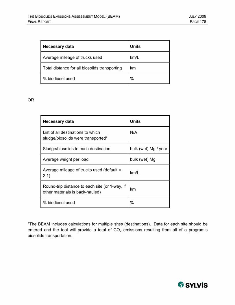
THE BIOSOLIDS EMISSIONS ASSESSMENT MODEL (BEAM) JULY 2009 FINAL REPORT PAGE 178
Necessary data Units
Average mileage of trucks used km/L
Total distance for all biosolids transporting km
% biodiesel used %
OR
Necessary data Units
List of all destinations to which sludge/biosolids were transported*
N/A
Sludge/biosolids to each destination bulk (wet) Mg / year
Average weight per load bulk (wet) Mg
Average mileage of trucks used (default = 2.1)
km/L
Round-trip distance to each site (or 1-way, if other materials is back-hauled)
km
% biodiesel used %
*The BEAM includes calculations for multiple sites (destinations). Data for each site should be entered and the tool will provide a total of CO2 emissions resulting from all of a program’s biosolids transportation.