the net climate impact of coal-ﬁred power plant … d. shindell and g. faluvegi: the net climate...

Atmos. Chem. Phys., 10, 3247–3260, 2010www.atmos-chem-phys.net/10/3247/2010/© Author(s) 2010. This work is distributed underthe Creative Commons Attribution 3.0 License.

AtmosphericChemistry

and Physics

The net climate impact of coal-fired power plant emissions

D. Shindell and G. Faluvegi

NASA Goddard Institute for Space Studies and Columbia University, New York, NY, USA

Received: 1 September 2009 – Published in Atmos. Chem. Phys. Discuss.: 9 October 2009Revised: 23 March 2010 – Accepted: 24 March 2010 – Published: 6 April 2010

Abstract. Coal-fired power plants influence climate via boththe emission of long-lived carbon dioxide (CO2) and short-lived ozone and aerosol precursors. Using a climate model,we perform the first study of the spatial and temporal pat-tern of radiative forcing specifically for coal plant emissions.Without substantial pollution controls, we find that near-termnet global mean climate forcing is negative due to the well-known aerosol masking of the effects of CO2. Impositionof pollution controls on sulfur dioxide and nitrogen oxidesleads to a rapid realization of the full positive forcing fromCO2, however. Long-term global mean forcing from stable(constant) emissions is positive regardless of pollution con-trols. Emissions from coal-fired power plants until∼1970,including roughly 1/3 of total anthropogenic CO2 emissions,likely contributed little net global mean climate forcing dur-ing that period though they may have induce weak NorthernHemisphere mid-latitude (NHml) cooling. After that timemany areas imposed pollution controls or switched to low-sulfur coal. Hence forcing due to emissions from 1970 to2000 and CO2 emitted previously was strongly positive andcontributed to rapid global and especially NHml warming.Most recently, new construction in China and India has in-creased rapidly with minimal application of pollution con-trols. Continuation of this trend would add negative near-term global mean climate forcing but severely degrade airquality. Conversely, following the Western and Japanesepattern of imposing air quality pollution controls at a latertime could accelerate future warming rates, especially atNHmls. More broadly, our results indicate that due to spatialand temporal inhomogenaities in forcing, climate impacts ofmulti-pollutant emissions can vary strongly from region toregion and can include substantial effects on maximum rate-of-change, neither of which are captured by commonly usedglobal metrics. The method we introduce here to estimateregional temperature responses may provide additional in-sight.

Correspondence to:D. Shindell([email protected])

1 Introduction

Coal combustion currently produces roughly 27% of theworld’s energy, second only to crude oil, and is the largestsingle source of electricity (∼41%). Coal is also a majorindustrial and residential fuel in some countries. At currentconsumption rates, enough reserves are available to last morethan a century (Energy Information Administration, 2009;hereafter EIA, 2009). Nearly half the known reserves arein the US, China and India, countries with large projected in-creases in energy demand over coming decades. Coal-firedpower plants are also currently the least expensive powersource in cost to generators per kWh of electricity. Hencethere are enormous economic and socio-political incentivesto expanded construction of coal-fired power plants. How-ever, emissions from coal-fired plants have substantial im-pacts on both air quality and climate change. Large amountsof CO2 are emitted, which lead to warming of the Earthand associated climate changes. Coal-fired power plants alsoemit substantial amounts of sulfur dioxide (SO2), a precur-sor of fine particulate and acid rain, and of nitrogen oxides(NOx, which is NO+NO2), gases influencing troposphericozone and methane as well as particulate, in addition to pro-ducing other pollutants such as mercury and solid waste. Tro-pospheric ozone and particulate are both harmful to humanhealth, with ozone and sulfur-containing species also damag-ing to both managed and natural ecosystems, and both influ-ence climate.

Tropospheric ozone, methane, sulfate and nitrate aerosolsall change in response to NOx and SO2 emissions, whichwe term the “air quality pollutant” emissions. All theseconstituents influence climate. Methane responds indirectlyto changes in its oxidation rate induced by NOx and SO2emissions, and hence we include it along with the othershort-lived air quality pollutants though it is relatively long-lived. The balance between the positive radiative forcing(RF) (leading to warming) from CO2 and the sum of RFfrom the various shorter-lived species will determine the netRF due to emissions from coal-fired power plants. It is

Published by Copernicus Publications on behalf of the European Geosciences Union.

http://creativecommons.org/licenses/by/3.0/

3248 D. Shindell and G. Faluvegi: The net climate impact of coal-fired power plant emissions

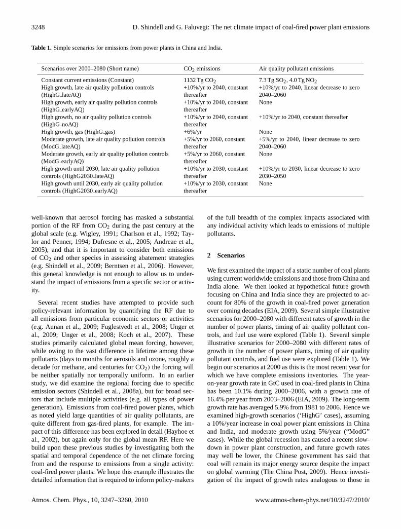
Table 1. Simple scenarios for emissions from power plants in China and India.

Scenarios over 2000–2080 (Short name) CO2 emissions Air quality pollutant emissions

Constant current emissions (Constant) 1132 Tg CO2 7.3 Tg SO2, 4.0 Tg NO2High growth, late air quality pollution controls(HighG lateAQ)

+10%/yr to 2040, constantthereafter

+10%/yr to 2040, linear decrease to zero2040–2060

High growth, early air quality pollution controls(HighG earlyAQ)


None

High growth, no air quality pollution controls(HighG noAQ)


+10%/yr to 2040, constant thereafter

High growth, gas (HighGgas) +6%/yr NoneModerate growth, late air quality pollution controls(ModG lateAQ)



Moderate growth, early air quality pollution controls(ModG earlyAQ)


None

High growth until 2030, late air quality pollutioncontrols (HighG2030lateAQ)



High growth until 2030, early air quality pollutioncontrols (HighG2030earlyAQ)


None

well-known that aerosol forcing has masked a substantialportion of the RF from CO2 during the past century at theglobal scale (e.g. Wigley, 1991; Charlson et al., 1992; Tay-lor and Penner, 1994; Dufresne et al., 2005; Andreae et al.,2005), and that it is important to consider both emissionsof CO2 and other species in assessing abatement strategies(e.g. Shindell et al., 2009; Berntsen et al., 2006). However,this general knowledge is not enough to allow us to under-stand the impact of emissions from a specific sector or activ-ity.

Several recent studies have attempted to provide suchpolicy-relevant information by quantifying the RF due toall emissions from particular economic sectors or activities(e.g. Aunan et al., 2009; Fuglestvedt et al., 2008; Unger etal., 2009; Unger et al., 2008; Koch et al., 2007). Thesestudies primarily calculated global mean forcing, however,while owing to the vast difference in lifetime among thesepollutants (days to months for aerosols and ozone, roughly adecade for methane, and centuries for CO2) the forcing willbe neither spatially nor temporally uniform. In an earlierstudy, we did examine the regional forcing due to specificemission sectors (Shindell et al., 2008a), but for broad sec-tors that include multiple activities (e.g. all types of powergeneration). Emissions from coal-fired power plants, whichas noted yield large quantities of air quality pollutants, arequite different from gas-fired plants, for example. The im-pact of this difference has been explored in detail (Hayhoe etal., 2002), but again only for the global mean RF. Here webuild upon these previous studies by investigating both thespatial and temporal dependence of the net climate forcingfrom and the response to emissions from a single activity:coal-fired power plants. We hope this example illustrates thedetailed information that is required to inform policy-makers

of the full breadth of the complex impacts associated withany individual activity which leads to emissions of multiplepollutants.

2 Scenarios

We first examined the impact of a static number of coal plantsusing current worldwide emissions and those from China andIndia alone. We then looked at hypothetical future growthfocusing on China and India since they are projected to ac-count for 80% of the growth in coal-fired power generationover coming decades (EIA, 2009). Several simple illustrativescenarios for 2000–2080 with different rates of growth in thenumber of power plants, timing of air quality pollutant con-trols, and fuel use were explored (Table 1). Several simpleillustrative scenarios for 2000–2080 with different rates ofgrowth in the number of power plants, timing of air qualitypollutant controls, and fuel use were explored (Table 1). Webegin our scenarios at 2000 as this is the most recent year forwhich we have complete emissions inventories. The year-on-year growth rate in GtC used in coal-fired plants in Chinahas been 10.1% during 2000–2006, with a growth rate of16.4% per year from 2003–2006 (EIA, 2009). The long-termgrowth rate has averaged 5.9% from 1981 to 2006. Hence weexamined high-growth scenarios (‘HighG’ cases), assuminga 10%/year increase in coal power plant emissions in Chinaand India, and moderate growth using 5%/year (“ModG”cases). While the global recession has caused a recent slow-down in power plant construction, and future growth ratesmay well be lower, the Chinese government has said thatcoal will remain its major energy source despite the impacton global warming (The China Post, 2009). Hence investi-gation of the impact of growth rates analogous to those in

Atmos. Chem. Phys., 10, 3247–3260, 2010 www.atmos-chem-phys.net/10/3247/2010/

D. Shindell and G. Faluvegi: The net climate impact of coal-fired power plant emissions 3249

past years seems warranted. For comparison, growth in en-ergy produced from coal between 2000 and 2050 in the SRESscenarios ranged from−78% to +679% (Nakicenovic et al.,2000). Our scenarios span +174% to +713% for this timeperiod, which overlaps fairly well with and covers a largeportion of the SRES range.

World coal reserves are estimated at 930 Gt coal (EIA,2009). In the high-growth scenario, usage grows very rapidlyas time progresses due to the geometric increase when ap-plying a constant percentage growth. We stop the increase inpower plant capacity when 1/4 of world reserves have beenused up solely by the additional usage in China and India(i.e. 232 Gt used), which is in year 40 for a 10%/yr growthrate. Maintaining constant usage after 2040 exhausts currentreserves at 2075 under that scenario. As the date at whichgrowth ceases has a strong effect on the total usage, we alsoinclude a high-growth scenario where growth terminates at2030 instead of 2040. Air quality pollution controls (removalof SO2 and NOx) are imposed either at the start of the sce-nario (“earlyAQ” cases) or at the end of the addition of coal-fired power plants (2030 or 2040; “lateAQ” cases). In theformer cases, we assume full air quality pollutant controlsare put in place as new plants are constructed, so there areno air quality pollutant emissions. In the latter, we assumeair quality pollutant controls are gradually retrofitted to theplants constructed since 2000 over 20 years (2031–2050 or2041–2060) during which time the SO2 and NOx emissionsboth decrease linearly to zero. An additional high-growthscenario never imposes pollution controls, even after all newconstruction ceases in 2040. This provides another view ofthe emissions of a constant number of power plants, as in thefirst “constant current emissions” case, but this time includ-ing the effects of the CO2 emissions during the earlier yearswhen the number of plants was increasing (i.e. RF at a giventime in this scenario after 2040 is due to SO2 and NOx emis-sions at that time plus the effect of all CO2 emitted from 2000to that time). In the moderate-growth scenarios, new plantsare added until 2060, but pollution controls are still imposedat 2040 (Table 1).

Finally, we include a scenario for comparison in whichgrowth of 10% per year in year 2000 coal-fired power ca-pacity is again assumed, but all additional capacity is gener-ated through natural gas rather than coal. CO2 emissions are15 kg C/GJ from gas-fired power plants, as compared with25 kg C/GJ from coal-fired plants (Ramanathan and Feng,2008), but virtually no SO2 or NOx is generated from gascombustion. Hence the effect is a 40% drop in CO2 emis-sions relative to coal and a complete removal of air qualitypollution effects. Note that neither coal- nor gas-fired powerplants emit substantial quantities of carbonaceous aerosols(black and organic carbon). In all scenarios, all emissionsother than these changes in power generation-related emis-sions are held fixed as we wish to examine the RF due tothese emissions alone.

Table 2. Year 2000 emissions from coal-fired power generation (Tgor Mt).

China India US

CO2 771 361 2442 (2517)SO2 5.4 1.9 12.0 (9.0)NOx 2.7 1.3 5.6 (3.7)

Footnotes to Table 2: Emissions are in Tg CO2, Tg SO2 andTg NO2. Conversion from PJ coal used for power to emissionsbased on 29.3 GJ per ton of coal. Emission factors are 16 gSO2/kg coal for China and 12 g/kg for India, 8 g NO2/kg coal forboth, and 2278 g CO2/kg coal for both based on mid-range values(Streets et al., 2003). US data is also given for 2007 in paren-theses (US data from EIA, 2009) (http://www.eia.doe.gov/cneaf/electricity/epa/epates.html).

3 Experimental setup

We examined the radiative forcing relative to the year 2000due to these hypothetical scenarios for emissions of CO2,SO2 and NOx. We first performed full three-dimensionalchemistry-climate model calculations of the effect of increas-ing SO2 and NOx from China and India. In these calcu-lations, aerosol and ozone precursor emissions from coal-fired power plants were increased throughout China (20–48 N, 100–125 E) and India (5–30 N, 65–90 E). Base caseemissions for all species and sectors are the 2000 inventoryof the International Institute for Applied Systems Analysis(IIASA) which is based on the 1995 EDGAR3.2 inventory,extrapolated to 2000 using national and sector economic de-velopment data (Dentener et al., 2005). For the power sec-tor, the IIASA inventory provides the spatial distribution ofemissions. The magnitude of emissions specifically originat-ing in coal-fired power generation is taken from a detailedspecies- and sector-specific 2000 inventory for Asia (Streetset al., 2003) (Table 2).

Calculations were performed using the composition-climate model G-PUCCINI to calculate the atmosphericcomposition response to the SO2 and NOx emissions changesand their radiative forcing. This model incorporates gas-phase (Shindell et al., 2006), sulfate (Koch et al., 2006) andnitrate (Bauer et al., 2007) aerosol chemistry within the GISSModelE general circulation model (Schmidt et al., 2006).The model used here has 23 vertical layers and 4 by 5 degreehorizontal resolution. Evaluations of the present-day compo-sition in the model against observations are generally quitereasonable (as documented in the references given above).The model was initially integrated for 5 years to allow adjust-ment of ozone and aerosol concentrations to emissions. An-nual average all-sky aerosol optical depths (AOD) during theinitial 5-yr period are 0.040 for sulfate and 0.020 for nitrate.A recent comparison of multiple models (Schulz et al., 2006)shows a mean sulfate AOD of 0.035 (range 0.015 to 0.055),

www.atmos-chem-phys.net/10/3247/2010/ Atmos. Chem. Phys., 10, 3247–3260, 2010

http://www.eia.doe.gov/cneaf/electricity/epa/epates.html

http://www.eia.doe.gov/cneaf/electricity/epa/epates.html


2080

0.15

0.1

0.05

0

-0.05

-0.1

Rad

iativ

e F

orci

ng (

W/m

2 )

OzoneMethane

Sulfate(direct)

Nitrate

Total

Sulfate(direct+indirect)

Carbondioxide

-0.4

-0.2

0

.2

.4

.6

2080

Year

2080-0.1

indirect)

-0.4

-0.2

0

.2

.4

.6

2080

Year YY

Rad

iativ

e F

orci

ng (

W/m

2 )

Total

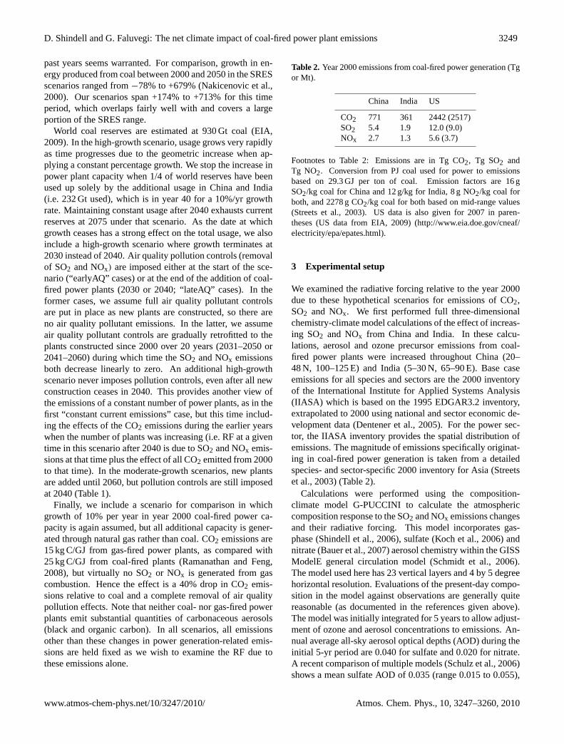
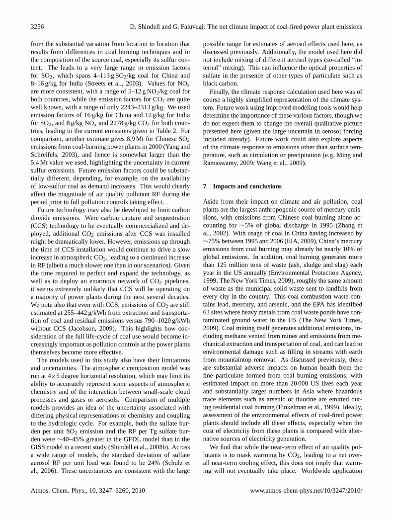
Fig. 1. Timeseries of global mean annual average radiative forcingfor the case of constant emissions from coal burning power plants.Emissions are year 2000 emissions in China and India (upper panel)and worldwide from coal-burning power plants (lower panel). In theupper panel, values are shown for individual forcing agents as wellas for the total forcing, with all values relative to 2000 and includingonly emissions from 2000 onward. Forcings are adjusted values atthe tropopause (in all figures).

so that our values are mid-range. Observational constraintson the all-sky value are not readily available, as most of theextant measurement techniques are reliable only in clear-sky(cloud-free) conditions. Sampling clear-sky areas only, themodel’s global total AOD for all species is 0.14, while ob-servations give global mean values of 0.135 (ground-basedAERONET) or 0.15 (satellite composites), though these havesubstantial limitations in their coverage (Kinne et al., 2006).The radiative forcing per unit burden change in this modelhas been discussed and compared with other models previ-ously (Shindell et al., 2008b; Schulz et al., 2006) (see dis-cussion in Sect. 6). Following initialization, the compositionresponse to increasing emissions was simulated from 2000 to2040.

The direct RF due to ozone and aerosols was calculatedinternally within the climate model. Aerosol indirect effects(AIE) are highly uncertain (Penner et al., 2006; Forster etal., 2007) and hence not robustly characterized using a sin-gle model. To provide a rough idea of the magnitude of po-tential AIE, we include their effect using the conservativeestimate that they are equal to the direct effect from sulfateaerosols. Calculations based on detailed modeling and ob-

servations suggest that the ratio of AIE to direct sulfate RF is1.5 to 2.0 (Kvalevag and Myhre, 2007), but we use a lowervalue of 1.0 as AIE may saturate at the very large regionalsulfate loadings reached in our simulations, and recent anal-yses based on satellite data suggest that at least a portion ofthe AIE may be fairly weak (Quaas et al., 2008). We includean uncertainty of a factor of three in the AIE estimate (50%),similar to the ranges given in recent assessments (Penner etal., 2006; Forster et al., 2007) and large enough to reasonablycharacterize the overall uncertainty in sulfate aerosol forc-ing. Uncertainties in greenhouse gas forcings are neglectedas these are very small in comparison with aerosol-relatedforcing uncertaintes.

The response to CO2 emissions was calculated using im-pulse response functions derived from the Bern Carbon Cy-cle Model (Siegenthaler and Joos, 1992) based on the versionused in the IPCC TAR. Exponential fits to those functionsare used to calculate the CO2 concentration at a given yearresulting from all emissions in prior years. This approach isexpected to yield fairly similar results to a more sophisticatedcarbon cycle model for the cases studied here, at least untilthe latter part of the 21st century when CO2 level becomesubstantially larger in some scenarios and could induce ad-ditional feedbacks. We also perform an offline calculation ofthe steady-state methane response to changes in modeled ox-idants, as in prior work (Shindell et al., 2008a). As methaneis prescribed at present-day values in the chemistry model,changes in modeled methane oxidation result solely fromchanges in oxidizing agents, and fully capture spatial andseasonal variations. We also include the feedback of methaneon its own lifetime (usingδln(OH)=−0.32δln(CH4) as rec-ommended in Prather et al., 2001). We include the slow re-sponse of ozone to the decadal timescale changes in methane,the so-called primary mode ozone (Wild et al., 2001), basedon prior modeling (Shindell et al., 2005). Radiative forc-ing from CO2 and methane are calculated using the standardIPCC TAR formulation (Ramaswamy et al., 2001). All val-ues are adjusted forcing (allowing stratospheric temperaturesto respond) at the tropopause.

4 Radiative forcing results

We first examine the net radiative forcing from CO2, sulfate,ozone, methane and nitrate for the reference cases of con-stant emissions from power plants. These cases include onlyemissions from the present and future, and do not accountfor any prior emissions from these plants. They thus pro-vide a reference for the effect of newly added plants, or forthe effect of those emissions that can still be affected by pol-icy for existing plants. The influence of historical emissionsfrom current plants is discussed later (Sect. 5). Using cur-rent emissions from China and India that are largely withoutpollution controls (Fig. 1; upper panel), we see that there isan immediate negative overall forcing that slowly decreases



with time and eventually turns into a positive forcing as CO2accumulates in the atmosphere. In addition to CO2, forcingis dominated by the direct and indirect effects of increasedsulfate aerosol (due to the SO2 emissions), with a small addi-tion from reduced methane (due to increased NOx and henceozone and OH). There are very small positive forcings fromincreased ozone (due to the NOx emissions) and decreasednitrate aerosol. The latter arises from a greater formation ofammonium sulfate at the expense of ammonium nitrate (asthere is competition for the limited supply of ammonium).The net result is that the short-term climate impact of coalburning in power plants without pollution controls is oppo-site to the long-term impact, with the transition time (∼20–40 years) highly dependent upon the magnitude of the AIE.Note that the results were highly linear despite pollutant in-creases up to a factor of 40. However, photochemical regimes(sunlight and cloud cover, temperature, removal rates, etc.)and background concentrations do vary with geographic lo-cation, and can lead to differences as large as a factor of 2 inthe RF per unit SO2 emission change (Shindell et al., 2008a).Thus our results are specific to emissions from Asia, thoughtypically regional differences are fairly small and well withinthe uncertainty ranges given here. Hence these results canalso provide a fairly rough estimate for the instantaneous RFof US (or European) emissions during the early 1970s, whichwere comparable in magnitude to those from China and Indiain 2000.

To put the future forcing from added power plants in con-text, we also show the total forcing from current worldwideemissions from coal-burning power plants (Fig. 1; lowerpanel). In this case, we have assumed that air quality pol-lutant emissions per Gt coal burnt in other OECD countriesare comparable to those in the US and in other non-OECDcountries they are comparable to those in India. Total coaluse was taken from EIA (2009). Results are similar to thosefor China and India alone but with greater magnitude andan earlier transfer time from negative to positive forcing dueto the presence of air quality pollutant emission controls inmany parts of the world. These results are not intended tobe a control scenario, but instead serve as references for con-stant current emissions to allow comparison of the effects ofnew plants with those of existing plants and to see how forc-ing from a particular plant changes with time.

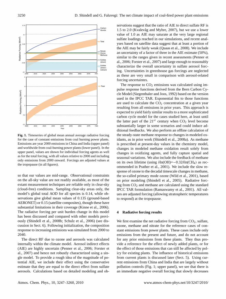
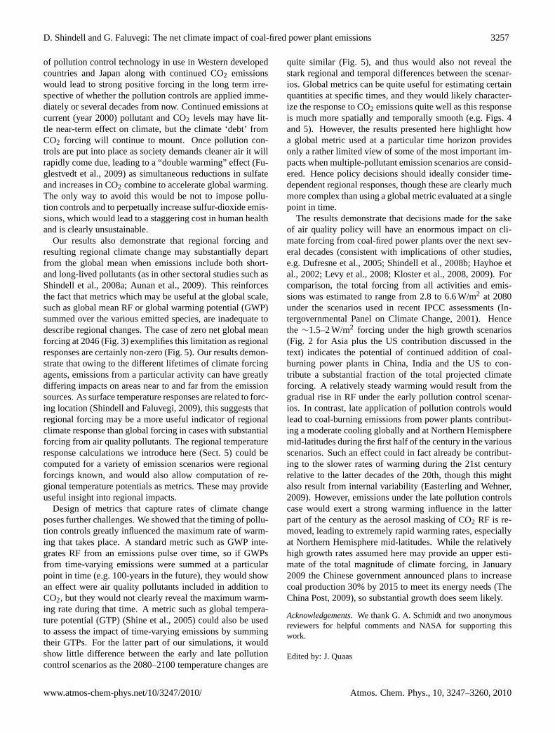
We next examine results from the hypothetical scenariosfor additional plants in China and India (Fig. 2). The high-growth scenarios show that the timing at which pollutantcontrols are imposed has an enormous effect on the net RFover the next several decades. The HighGearlyAQ scenarioshows a net forcing of nearly 0.7 W/m2 at 2040, while theHighG lateAQ scenario has a forcing in the range of−0.3 to−1.0 W/m2. Hence until they are controlled, the air qualitypollutants emitted by a steadily increasing number of powerplants exert an even more powerful, but opposite sign, globalmean forcing than the CO2 emissions. However, the timingof pollution controls has no effect on the radiative forcing

2080

Year

Rad

iativ

e F

orci

ng (

W/m

2 )

Fig. 2. Timeseries of global mean annual average radiative forcingrelative to the year 2000 in the various indicated scenarios. Note thatthe high growth scenarios are shown in red-orange-green colors andthe moderate growth in blues. Forcing is the sum of contributionsfrom carbon dioxide, sulfate, ozone, methane and nitrate. Dashedlines are those scenarios with substantial aerosol forcing (late or nopollution controls). The shaded region shows the uncertainty asso-ciated with aerosol forcing in the “Highlate” case as an example.All the dashed lines would have comparable uncertainty ranges (theothers are omitted for visual clarity).

once those controls are fully in place, leading to identicalvalues past 2060 in the earlyAQ and lateAQ high-growth sce-narios (there will be an effect on the integrated RF felt by theEarth however, which will impact the trajectory of the sur-face temperature climate response even if not the final state,as discussed in Sect. 5). The high-growth scenarios show acontinued increase in RF throughout the period studied de-spite constant emissions after 2040. The continued increase,which is still fairly rapid at 2080 (0.25 W/m2 per decade) re-sults from the long adjustment time of atmospheric CO2 toemissions.

The high-growth scenarios in which growth ceases at 2030instead of 2040 show substantially less forcing during thelatter part of the century. Forcing at 2080 is roughly half incomparison with the scenarios in which growth persists until2040. A large impact is not surprising given that adding 10%per year coal-fired power generation capacity from 2030–2039 increases annual average total coal usage by 260%.

The overall growth rate (high vs. moderate) has a greaterimpact on the forcing in our various scenarios in the laterdecades than the year at which growth ceases or even whetherair quality pollution controls are imposed at all. A more mod-est 5% per year growth rate all the way though 2060 leads to60% less RF at 2080 than a 10% per year growth rate through2040. Use of gas instead of coal also leads to decreased forc-ing, but not as dramatic a reduction as lowering the growthrate by half.



.2 .5 2.5 5 10-.2-.5-2.5-5-10Radiative forcing (W/m2)

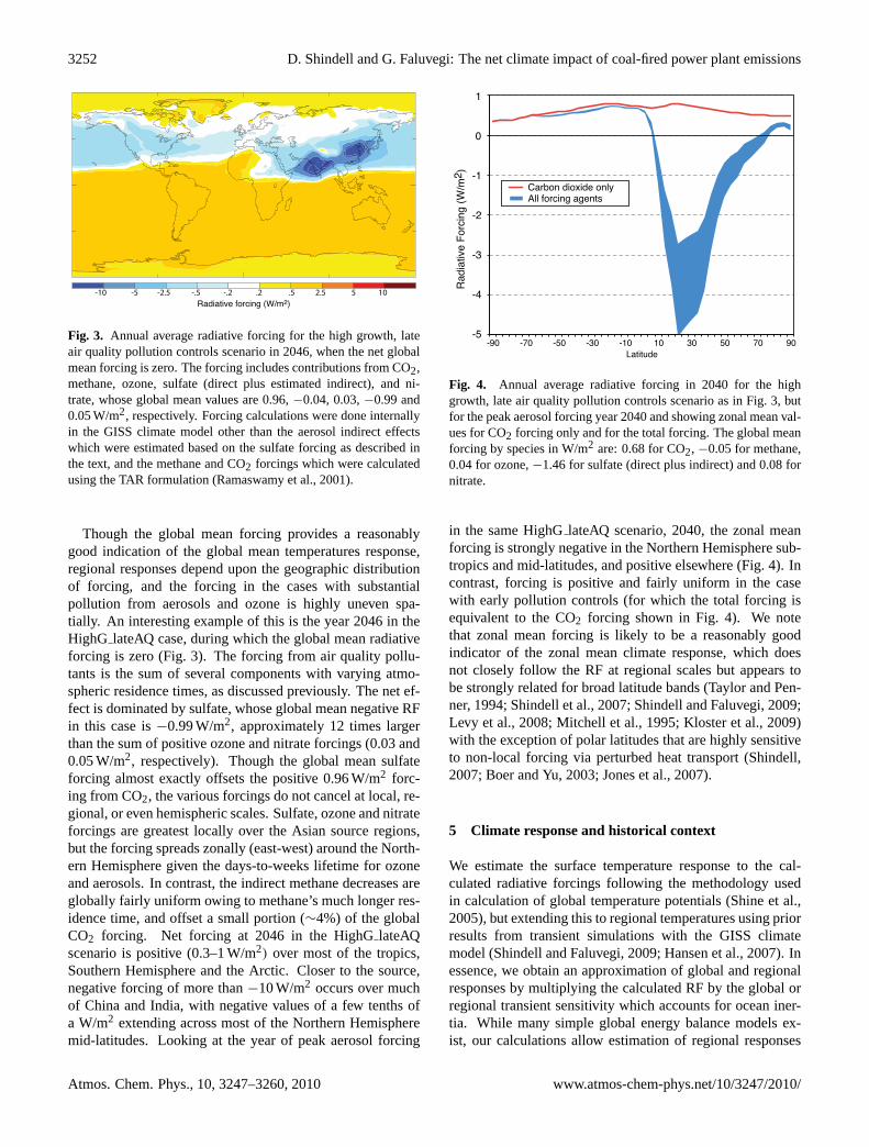
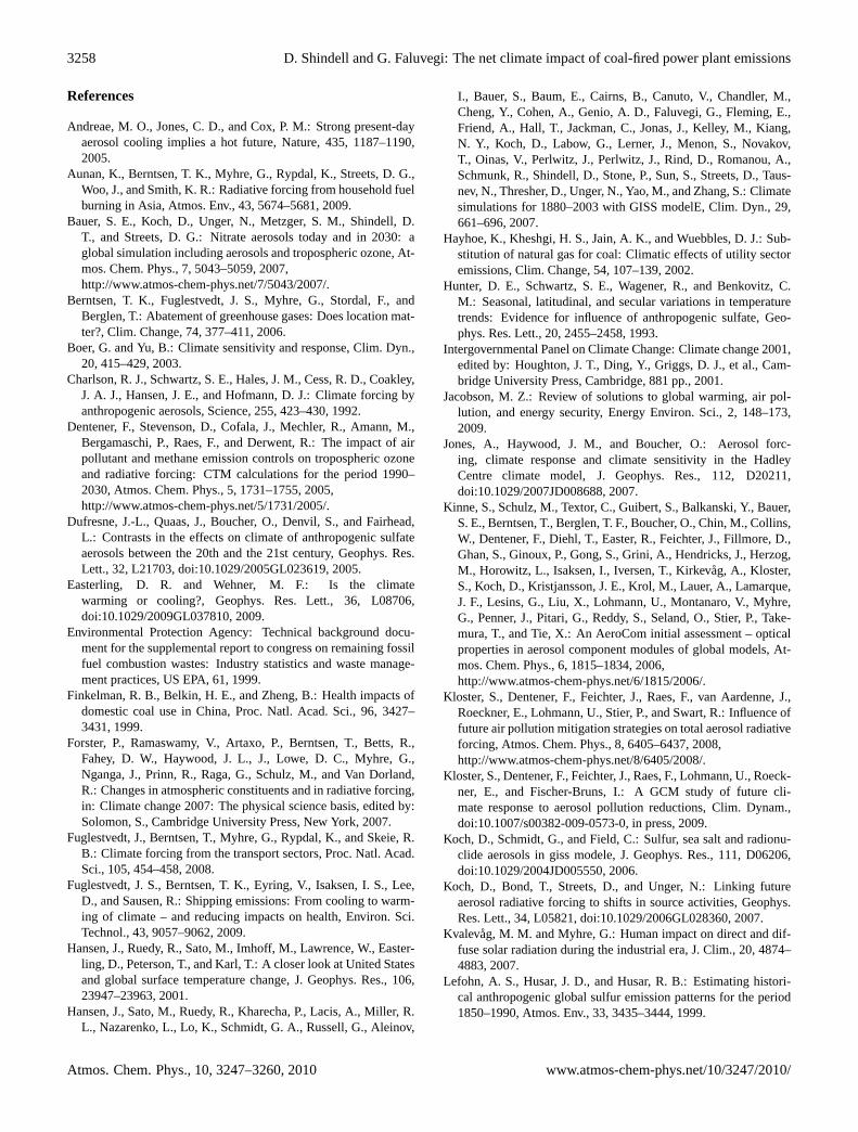
Fig. 3. Annual average radiative forcing for the high growth, lateair quality pollution controls scenario in 2046, when the net globalmean forcing is zero. The forcing includes contributions from CO2,methane, ozone, sulfate (direct plus estimated indirect), and ni-trate, whose global mean values are 0.96,−0.04, 0.03,−0.99 and0.05 W/m2, respectively. Forcing calculations were done internallyin the GISS climate model other than the aerosol indirect effectswhich were estimated based on the sulfate forcing as described inthe text, and the methane and CO2 forcings which were calculatedusing the TAR formulation (Ramaswamy et al., 2001).

Though the global mean forcing provides a reasonablygood indication of the global mean temperatures response,regional responses depend upon the geographic distributionof forcing, and the forcing in the cases with substantialpollution from aerosols and ozone is highly uneven spa-tially. An interesting example of this is the year 2046 in theHighG lateAQ case, during which the global mean radiativeforcing is zero (Fig. 3). The forcing from air quality pollu-tants is the sum of several components with varying atmo-spheric residence times, as discussed previously. The net ef-fect is dominated by sulfate, whose global mean negative RFin this case is−0.99 W/m2, approximately 12 times largerthan the sum of positive ozone and nitrate forcings (0.03 and0.05 W/m2, respectively). Though the global mean sulfateforcing almost exactly offsets the positive 0.96 W/m2 forc-ing from CO2, the various forcings do not cancel at local, re-gional, or even hemispheric scales. Sulfate, ozone and nitrateforcings are greatest locally over the Asian source regions,but the forcing spreads zonally (east-west) around the North-ern Hemisphere given the days-to-weeks lifetime for ozoneand aerosols. In contrast, the indirect methane decreases areglobally fairly uniform owing to methane’s much longer res-idence time, and offset a small portion (∼4%) of the globalCO2 forcing. Net forcing at 2046 in the HighGlateAQscenario is positive (0.3–1 W/m2) over most of the tropics,Southern Hemisphere and the Arctic. Closer to the source,negative forcing of more than−10 W/m2 occurs over muchof China and India, with negative values of a few tenths ofa W/m2 extending across most of the Northern Hemispheremid-latitudes. Looking at the year of peak aerosol forcing

Carbon dioxide onlyAll forcing agents

Rad

iativ

e F

orci

ng (

W/m

2 )

-90 -70 -50 -30 -10 10 30 50 70 90 Latitude

0

1

-1

-2

-3

-4

-5

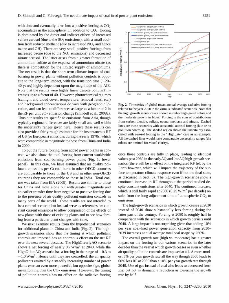
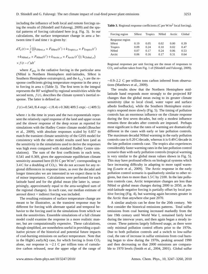
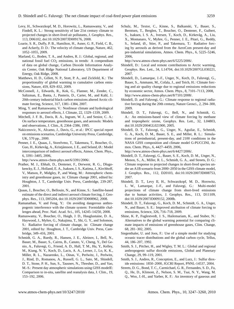
Fig. 4. Annual average radiative forcing in 2040 for the highgrowth, late air quality pollution controls scenario as in Fig. 3, butfor the peak aerosol forcing year 2040 and showing zonal mean val-ues for CO2 forcing only and for the total forcing. The global meanforcing by species in W/m2 are: 0.68 for CO2, −0.05 for methane,0.04 for ozone,−1.46 for sulfate (direct plus indirect) and 0.08 fornitrate.

in the same HighGlateAQ scenario, 2040, the zonal meanforcing is strongly negative in the Northern Hemisphere sub-tropics and mid-latitudes, and positive elsewhere (Fig. 4). Incontrast, forcing is positive and fairly uniform in the casewith early pollution controls (for which the total forcing isequivalent to the CO2 forcing shown in Fig. 4). We notethat zonal mean forcing is likely to be a reasonably goodindicator of the zonal mean climate response, which doesnot closely follow the RF at regional scales but appears tobe strongly related for broad latitude bands (Taylor and Pen-ner, 1994; Shindell et al., 2007; Shindell and Faluvegi, 2009;Levy et al., 2008; Mitchell et al., 1995; Kloster et al., 2009)with the exception of polar latitudes that are highly sensitiveto non-local forcing via perturbed heat transport (Shindell,2007; Boer and Yu, 2003; Jones et al., 2007).

5 Climate response and historical context

We estimate the surface temperature response to the cal-culated radiative forcings following the methodology usedin calculation of global temperature potentials (Shine et al.,2005), but extending this to regional temperatures using priorresults from transient simulations with the GISS climatemodel (Shindell and Faluvegi, 2009; Hansen et al., 2007). Inessence, we obtain an approximation of global and regionalresponses by multiplying the calculated RF by the global orregional transient sensitivity which accounts for ocean iner-tia. While many simple global energy balance models ex-ist, our calculations allow estimation of regional responses



including the influence of both local and remote forcings us-ing the results of (Shindell and Faluvegi, 2009) and the spa-tial patterns of forcing calculated here (e.g. Fig. 3). In ourcalculations, the surface temperature change in areaa be-tween time 0 and timet is given by:

dTa(t) =t

∫0

((kSHext,a ×FSHext(t

′)+kTropics,a ×FTropics(t′)

+kNHml,a ×FNHml(t′)+kArctic,a ×FArctic(t

′))/kGlobal,a

)×f (t − t ′)dt ′

whereFarea is the radiative forcing in the particular area(NHml is Northern Hemisphere mid-latitudes, SHext isSouthern Hemisphere extratropics), and thekx,y’s are the re-sponse coefficients giving temperature response in the area yto forcing in area x (Table 3). The first term in the integralrepresents the RF weighted by regional sensitivities while thesecond term,f (t), describes the climate system’s inertial re-sponse. The latter is defined as:

f (t)=0.541/8.4 exp(−t/8.4)+0.368/409.5 exp(−t/409.5)

wheret is the time in years and the two exponentials repre-sent the relatively rapid response of the land and upper oceanand the slower response of the deep ocean as reported forsimulations with the Hadley Centre climate model (Boucheret al., 2009), with absolute responses scaled by 0.857 tomatch the transient climate sensitivity of the GISS model forconsistency with the other model results used here (and asthe sensitivity in the simulations used to derive the responseswas high even compared with standard Hadley Centre sim-ulations). The sum of the first coefficients in each term,0.541 and 0.369, gives the approximate equilibrium climatesensitivity assumed here (0.91 C per W/m2; corresponding to3.4 C for a doubling of CO2). We do not account for any re-gional differences in response times, as over the decadal andlonger timescales we are interested in we expect these to beof minor importance. Calculations were performed for eachlatitude band and for the global mean (the latter is, unsur-prisingly, approximately equal to the area-weighted sum ofthe regional changes). In each case, our median estimate ofaerosol direct + indirect forcing was included.

The resulting estimates of surface temperature change aremeant to be illustrative, as the transient response may bedifferent for forcing with alternate spatial and temporal be-havior to the forcing used in the simulations from which wetook the sensitivities. Ensemble simulations of a full climatemodel could examine the response in a more realistic man-ner, but are computationally expensive. These calculations,though simplified, are nonetheless useful in providing a qual-itative picture of the historical and potential future impactsof coal-burning emissions on surface temperature. Note thatin the HighGearlyAQ case, for which forcing is from CO2alone, our response is∼2.1 C per trillion tons of cumula-tive carbon released, near the upper edge of the range of

Table 3. Regional response coefficients (C per W/m2 local forcing).

Forcing region SHext Tropics NHml Arctic Global

Response regionSHext 0.19 0.05 0.02 0.00 0.39Tropics 0.09 0.24 0.10 0.02 0.47NHml 0.07 0.17 0.24 0.06 0.53Arctic 0.06 0.16 0.17 0.31 0.64

Regional responses per unit forcing are the mean of responses toCO2 and sulfate taken from Fig. 1 of (Shindell and Faluvegi, 2009).

∼0.9–2.2 C per trillion tons carbon inferred from observa-tions (Matthews et al., 2009).

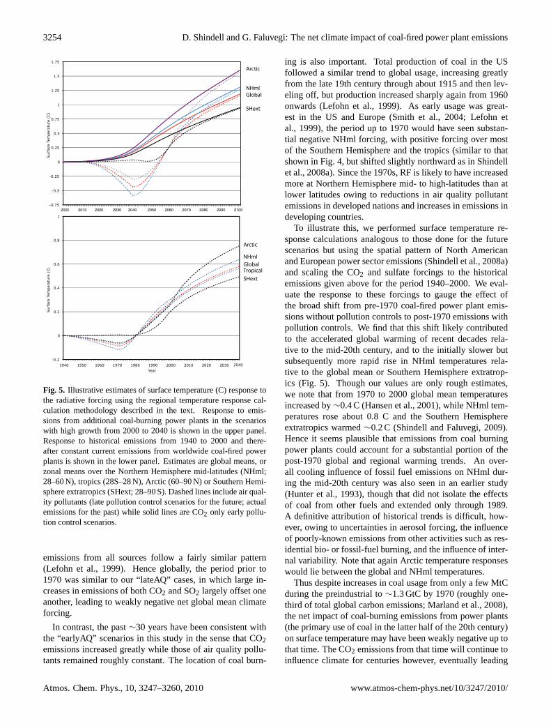
The results show that the Northern Hemisphere mid-latitude band responds more strongly to the projected RFchanges than the global mean owing to its greater climatesensitivity (due to local cloud, water vapor and surfacealbedo feedbacks), while the Southern Hemisphere extrat-ropics respond more slowly (Fig. 5). The timing of pollutioncontrols has an enormous influence on the climate responseduring the first seven decades, but only a modest influenceremains three decades after controls are imposed. Perhapsmost significant is that the rates of warming are dramaticallydifferent in the cases with early or late pollution controls.The maximum decadal NHml warming in the early pollutioncontrols case is 0.20 C/decade, whereas it is 0.49 C/decade inthe late pollution controls case. The tropics also experiencesconsiderably faster warming rates in the late pollution controlscenario than with early pollution controls (tropical warmingis very similar to the global mean values shown in Fig. 5).This may have profound effects on biological systems whichface increasing difficulty in adapting to more rapid warm-ing (Loarie et al., 2009). The Arctic response in the earlypollution control scenario is qualitatively similar to other re-gions, but rises to more than 1.5 C by 2100. In the late pollu-tion controls case, Arctic temperature changes are less thanNHml or global mean changes during 2000 to 2050, as themid-latitude negative forcing is partially offset by local pos-itive forcing (Fig. 4), but warming again becomes greater inthe Arctic than anywhere else past 2070.

A similar analysis can be done for the 20th century. Wefirst consider the historical emissions patterns. Total sulfuremissions from coal burning increased markedly from thelate 19th century until World War I, remained fairly levelduring the interwar years, and then again began a steady in-crease. These patterns largely followed usage, as there wereonly minimal pollution control efforts prior to the 1970s.Due to both pollution controls and a switch to low-sulfurcoal, the rate of increase in sulfur emissions from coal burn-ing began to slow during the 1970s, peaking around 1990and then decreasing so that 2000 emissions are compara-ble to 1970 levels (Smith et al., 2004, 2001). Global sulfur



2010 2020 2030 2040 2050 2060 2070 2080 2090 2100 2000 2010 2020 2030 2040 2050 2060 2070 2080 2090 21002000-0.75

-0.5

-0.25

0

0.25

0.5

0.75

1

1.25

1.5

1.75

Sur

face

Tem

pera

ture

(C)

Arctic

NHmlGlobal

SHext

2010 2020 2030 2040 2050 2060 2070 2080 2090 2100 2000

-0.2

0

0.2

0.4

0.6

0.8

1

1940 1950 1960 1970 1980 1990 2000 2010 2020 2030

Sur

face

Tem

pera

ture

(C)

Year

Arctic

NHmlGlobalTropicalSHext

2040

Fig. 5. Illustrative estimates of surface temperature (C) response tothe radiative forcing using the regional temperature response cal-culation methodology described in the text. Response to emis-sions from additional coal-burning power plants in the scenarioswith high growth from 2000 to 2040 is shown in the upper panel.Response to historical emissions from 1940 to 2000 and there-after constant current emissions from worldwide coal-fired powerplants is shown in the lower panel. Estimates are global means, orzonal means over the Northern Hemisphere mid-latitudes (NHml;28–60 N), tropics (28S–28 N), Arctic (60–90 N) or Southern Hemi-sphere extratropics (SHext; 28–90 S). Dashed lines include air qual-ity pollutants (late pollution control scenarios for the future; actualemissions for the past) while solid lines are CO2 only early pollu-tion control scenarios.

emissions from all sources follow a fairly similar pattern(Lefohn et al., 1999). Hence globally, the period prior to1970 was similar to our “lateAQ” cases, in which large in-creases in emissions of both CO2 and SO2 largely offset oneanother, leading to weakly negative net global mean climateforcing.

In contrast, the past∼30 years have been consistent withthe “earlyAQ” scenarios in this study in the sense that CO2emissions increased greatly while those of air quality pollu-tants remained roughly constant. The location of coal burn-

ing is also important. Total production of coal in the USfollowed a similar trend to global usage, increasing greatlyfrom the late 19th century through about 1915 and then lev-eling off, but production increased sharply again from 1960onwards (Lefohn et al., 1999). As early usage was great-est in the US and Europe (Smith et al., 2004; Lefohn etal., 1999), the period up to 1970 would have seen substan-tial negative NHml forcing, with positive forcing over mostof the Southern Hemisphere and the tropics (similar to thatshown in Fig. 4, but shifted slightly northward as in Shindellet al., 2008a). Since the 1970s, RF is likely to have increasedmore at Northern Hemisphere mid- to high-latitudes than atlower latitudes owing to reductions in air quality pollutantemissions in developed nations and increases in emissions indeveloping countries.

To illustrate this, we performed surface temperature re-sponse calculations analogous to those done for the futurescenarios but using the spatial pattern of North Americanand European power sector emissions (Shindell et al., 2008a)and scaling the CO2 and sulfate forcings to the historicalemissions given above for the period 1940–2000. We eval-uate the response to these forcings to gauge the effect ofthe broad shift from pre-1970 coal-fired power plant emis-sions without pollution controls to post-1970 emissions withpollution controls. We find that this shift likely contributedto the accelerated global warming of recent decades rela-tive to the mid-20th century, and to the initially slower butsubsequently more rapid rise in NHml temperatures rela-tive to the global mean or Southern Hemisphere extratrop-ics (Fig. 5). Though our values are only rough estimates,we note that from 1970 to 2000 global mean temperaturesincreased by∼0.4 C (Hansen et al., 2001), while NHml tem-peratures rose about 0.8 C and the Southern Hemisphereextratropics warmed∼0.2 C (Shindell and Faluvegi, 2009).Hence it seems plausible that emissions from coal burningpower plants could account for a substantial portion of thepost-1970 global and regional warming trends. An over-all cooling influence of fossil fuel emissions on NHml dur-ing the mid-20th century was also seen in an earlier study(Hunter et al., 1993), though that did not isolate the effectsof coal from other fuels and extended only through 1989.A definitive attribution of historical trends is difficult, how-ever, owing to uncertainties in aerosol forcing, the influenceof poorly-known emissions from other activities such as res-idential bio- or fossil-fuel burning, and the influence of inter-nal variability. Note that again Arctic temperature responseswould lie between the global and NHml temperatures.

Thus despite increases in coal usage from only a few MtCduring the preindustrial to∼1.3 GtC by 1970 (roughly one-third of total global carbon emissions; Marland et al., 2008),the net impact of coal-burning emissions from power plants(the primary use of coal in the latter half of the 20th century)on surface temperature may have been weakly negative up tothat time. The CO2 emissions from that time will continue toinfluence climate for centuries however, eventually leading



to a substantial warming. This can be seen in the strongwarming response during 2000 to 2040 that results from thecombined effect of historical emissions of CO2 and constantyear 2000 emissions (Fig. 5; lower panel). It’s clear that thiswarming is driven by the response to pre-2000 emissions ofCO2 since the forcing from constant current emissions aloneis negative for the 2000–2020 period (Fig. 1).

The influence of coal-burning in the early 20th centuryis more difficult to assess. The rapid increase in US coalusage from∼1900, when it was∼200 Mt, to 1915, whenit reached∼550 Mt (EIA, 2009), was accompanied by con-comitant increases in sulfur emissions which likely maskedmuch of the warming from CO2. However, coal usage at thattime primarily consisted of residential and industrial uses,not electricity generation. These types of combustion aretypically much less complete, and hence emit large quanti-ties of black carbon, a powerful positive short-lived radiativeforcing agent. Consistent with this, the abundance of blackcarbon in ice cores from Greenland, downwind of the US,peaks in the early 20th century (McConnell et al., 2007).Hence even if the warming effect of CO2 was largely off-set by increased sulfur emissions, the net effect of emissionsfrom the rapid increase in early 20th century coal burningwould likely have been a positive RF. This may have con-tributed to the observed global and regional warming duringroughly 1915–1930 (assuming a 1–2 decade lag in climateresponse to forcing). From∼1950 to 2000, usage of coal togenerate electricity increased from∼20% of the total US us-age to∼90% (it was∼54% in China in 2000, and∼70% inIndia). Hence current emissions from coal burning withoutpollution controls are much more likely to have near-zero netshort-term forcing than those of the early 20th century.

6 Uncertainties and limitations

There are many sources of uncertainty in estimating the cli-mate impact of future emissions, including the emission sce-narios, the emissions themselves, the chemistry model andthe climate response calculations. Beginning with the sce-narios, the socio-economic factors that govern future growthrates cannot be reliably predicted and emissions projectionsare based on many assumptions. While we investigated twopossible growth rates to explore sensitivity, actual trends willvary from either of those idealized projections. Under thehigh growth scenario, coal usage is 9.6 Gt coal in China andIndia for power generation at 2030, while under the moderategrowth scenario it is 2.3 Gt coal. EIA projections have 3.8 Gtcoal usage by China at 2030 and 0.6 Gt coal by India for allpurposes (∼60–70% of current coal usage in China and Indiais for power (Streets et al., 2003), so∼2.6–3.1 Gt of the to-tal), so our scenarios bracket those projections although ourmoderate scenario is much closer. The EIA projected growthrate for China decreases from 6% during 2005–2010 to lessthan 3% after 2015, however. As noted previously, histori-

cal growth rates have been substantially greater, so it is notobvious which path will be closer to actual future emissions.

Our scenarios also assume that when air quality pollutantcontrols are introduced, they are 100% effective. Thoughthis is clearly unrealistic, the impact of residual emissionswhen controls are in place is likely to be quite small basedon current US emissions and trends. Current air quality pol-lutant emissions from US coal-fired power plants create anannual average RF of less than 0.1 W/m2 despite CO2 emis-sions more than double those of China and India (Table 2).More importantly, from 1998 to 2007, US emissions of SO2and NOx decreased by∼30% and 40%, respectively. Thisoccurred despite an overall growth in coal usage (resulting inCO2 emissions increasing by∼7%) and air quality pollutantemissions in 1998 that were already quite reduced comparedwith 1970s levels. Further decreases are expected, demon-strating that technology exists to remove the vast majorityof SO2 and NOx emissions, so that the RF from residual airquality pollutant emissions if strict controls were put in placewould be very small.

Our scenarios were also limited in that they explored onlythe impact of hypothetical additional emissions from Chinaand India. EIA projections of total coal usage for 2005 to2030 show 80% of total growth in these two countries, withthe remainder divided nearly equally between the US and thedeveloping world (the latter mostly in other Asian countries).It is not completely clear how much of this growth is due tousage in power plants, however, and residential and indus-trial use of coal may have rather different effects as it alsoleads to substantial emissions of carbon monoxide, black andorganic carbon. Nonetheless, we can roughly estimate thecontributions from other regions. The contribution of ad-ditional coal burning plants in Asia would add∼10–15%to the estimated contribution from China and India usingthe EIA growth rates. The contribution of added US powerplants, which are projected to grow at 1.1%/yr (EIA, 2009)and we assume generate exclusively CO2 emissions, wouldbe an additional RF of 0.08 W/m2 at 2030 and 0.19 W/m2 at2080 from plants added between 2005 and 2030. Hence toget an estimate of the global forcing from worldwide addi-tion of coal-fired power plants,∼20–40% would be addedto the total 2080 forcing from power plants in China and In-dia, depending upon the scenario assumed for those coun-tries (Fig. 2). An estimate of the total forcing from coal-fired power plants should also include the forcing from ex-isting power plants worldwide. This adds roughly another0.4 W/m2 at 2080, though the value would be higher if pollu-tion controls were improved on existing plants; with a maxi-mum addition of∼0.25 W/m2 if all current air quality pollu-tant emissions were eliminated (Fig. 1). However, the valuecould also be lower if plants are taken out of commission,but again, neither future application of pollutant controls norplant lifetimes cannot be reliably projected.

Another large source of uncertainty is our incompleteknowledge of the emission factors for coal combustion and



from the substantial variation from location to location thatresults from differences in coal burning techniques and inthe composition of the source coal, especially its sulfur con-tent. The leads to a very large range in emission factorsfor SO2, which spans 4–113 g SO2/kg coal for China and8–16 g/kg for India (Streets et al., 2003). Values for NOxare more consistent, with a range of 5–12 g NO2/kg coal forboth countries, while the emission factors for CO2 are quitewell known, with a range of only 2243–2313 g/kg. We usedemission factors of 16 g/kg for China and 12 g/kg for Indiafor SO2, and 8 g/kg NOx and 2278 g/kg CO2 for both coun-tries, leading to the current emissions given in Table 2. Forcomparison, another estimate gives 8.9 Mt for Chinese SO2emissions from coal-burning power plants in 2000 (Yang andSchreifels, 2003), and hence is somewhat larger than the5.4 Mt value we used, highlighting the uncertainty in currentsulfur emissions. Future emission factors could be substan-tially different, depending, for example, on the availabilityof low-sulfur coal as demand increases. This would clearlyaffect the magnitude of air quality pollutant RF during theperiod prior to full pollution controls taking effect.

Future technology may also be developed to limit carbondioxide emissions. Were carbon capture and sequestration(CCS) technology to be eventually commercialized and de-ployed, additional CO2 emissions after CCS was installedmight be dramatically lower. However, emissions up throughthe time of CCS installation would continue to drive a slowincrease in atmospheric CO2, leading to a continued increasein RF (albeit a much slower one than in our scenarios). Giventhe time required to perfect and expand the technology, aswell as to deploy an enormous network of CO2 pipelines,it seems extremely unlikely that CCS will be operating ona majority of power plants during the next several decades.We note also that even with CCS, emissions of CO2 are stillestimated at 255–442 g/kWh from extraction and transporta-tion of coal and residual emissions versus 790–1020 g/kWhwithout CCS (Jacobson, 2009). This highlights how con-sideration of the full life-cycle of coal use would become in-creasingly important as pollution controls at the power plantsthemselves become more effective.

The models used in this study also have their limitationsand uncertainties. The atmospheric composition model wasrun at 4×5 degree horizontal resolution, which may limit itsability to accurately represent some aspects of atmosphericchemistry and of the interaction between small-scale cloudprocesses and gases or aerosols. Comparison of multiplemodels provides an idea of the uncertainty associated withdiffering physical representations of chemistry and couplingto the hydrologic cycle. For example, both the sulfate bur-den per unit SO2 emission and the RF per Tg sulfate bur-den were∼40–45% greater in the GFDL model than in theGISS model in a recent study (Shindell et al., 2008b). Acrossa wide range of models, the standard deviation of sulfateaerosol RF per unit load was found to be 24% (Schulz etal., 2006). These uncertainties are consistent with the large

possible range for estimates of aerosol effects used here, asdiscussed previously. Additionally, the model used here didnot include mixing of different aerosol types (so-called “in-ternal” mixing). This can influence the optical properties ofsulfate in the presence of other types of particulate such asblack carbon.

Finally, the climate response calculation used here was ofcourse a highly simplified representation of the climate sys-tem. Future work using improved modeling tools would helpdetermine the importance of these various factors, though wedo not expect them to change the overall qualitative picturepresented here (given the large uncertain in aerosol forcingincluded already). Future work could also explore aspectsof the climate response to emissions other than surface tem-perature, such as circulation or precipitation (e.g. Ming andRamaswamy, 2009; Wang et al., 2009).

7 Impacts and conclusions

Aside from their impact on climate and air pollution, coalplants are the largest anthropogenic source of mercury emis-sions, with emissions from Chinese coal burning alone ac-counting for∼5% of global discharge in 1995 (Zhang etal., 2002). With usage of coal in China having increased by∼75% between 1995 and 2006 (EIA, 2009), China’s mercuryemissions from coal burning may already be nearly 10% ofglobal emissions. In addition, coal burning generates morethan 125 million tons of waste (ash, sludge and slag) eachyear in the US annually (Environmental Protection Agency,1999; The New York Times, 2009), roughly the same amountof waste as the municipal solid waste sent to landfills fromevery city in the country. This coal combustion waste con-tains lead, mercury, and arsenic, and the EPA has identified63 sites where heavy metals from coal waste ponds have con-taminated ground water in the US (The New York Times,2009). Coal mining itself generates additional emissions, in-cluding methane vented from mines and emissions from me-chanical extraction and transportation of coal, and can lead toenvironmental damage such as filling in streams with earthfrom mountaintop removal. As discussed previously, thereare substantial adverse impacts on human health from thefine particulate formed from coal burning emissions, withestimated impact on more than 20 000 US lives each yearand substantially larger numbers in Asia where hazardoustrace elements such as arsenic or fluorine are emitted dur-ing residential coal burning (Finkelman et al., 1999). Ideally,assessment of the environmental effects of coal-fired powerplants should include all these effects, especially when thecost of electricity from these plants is compared with alter-native sources of electricity generation.

We find that while the near-term effect of air quality pol-lutants is to mask warming by CO2, leading to a net over-all near-term cooling effect, this does not imply that warm-ing will not eventually take place. Worldwide application



of pollution control technology in use in Western developedcountries and Japan along with continued CO2 emissionswould lead to strong positive forcing in the long term irre-spective of whether the pollution controls are applied imme-diately or several decades from now. Continued emissions atcurrent (year 2000) pollutant and CO2 levels may have lit-tle near-term effect on climate, but the climate ‘debt’ fromCO2 forcing will continue to mount. Once pollution con-trols are put into place as society demands cleaner air it willrapidly come due, leading to a “double warming” effect (Fu-glestvedt et al., 2009) as simultaneous reductions in sulfateand increases in CO2 combine to accelerate global warming.The only way to avoid this would be not to impose pollu-tion controls and to perpetually increase sulfur-dioxide emis-sions, which would lead to a staggering cost in human healthand is clearly unsustainable.

Our results also demonstrate that regional forcing andresulting regional climate change may substantially departfrom the global mean when emissions include both short-and long-lived pollutants (as in other sectoral studies such asShindell et al., 2008a; Aunan et al., 2009). This reinforcesthe fact that metrics which may be useful at the global scale,such as global mean RF or global warming potential (GWP)summed over the various emitted species, are inadequate todescribe regional changes. The case of zero net global meanforcing at 2046 (Fig. 3) exemplifies this limitation as regionalresponses are certainly non-zero (Fig. 5). Our results demon-strate that owing to the different lifetimes of climate forcingagents, emissions from a particular activity can have greatlydiffering impacts on areas near to and far from the emissionsources. As surface temperature responses are related to forc-ing location (Shindell and Faluvegi, 2009), this suggests thatregional forcing may be a more useful indicator of regionalclimate response than global forcing in cases with substantialforcing from air quality pollutants. The regional temperatureresponse calculations we introduce here (Sect. 5) could becomputed for a variety of emission scenarios were regionalforcings known, and would also allow computation of re-gional temperature potentials as metrics. These may provideuseful insight into regional impacts.

Design of metrics that capture rates of climate changeposes further challenges. We showed that the timing of pollu-tion controls greatly influenced the maximum rate of warm-ing that takes place. A standard metric such as GWP inte-grates RF from an emissions pulse over time, so if GWPsfrom time-varying emissions were summed at a particularpoint in time (e.g. 100-years in the future), they would showan effect were air quality pollutants included in addition toCO2, but they would not clearly reveal the maximum warm-ing rate during that time. A metric such as global tempera-ture potential (GTP) (Shine et al., 2005) could also be usedto assess the impact of time-varying emissions by summingtheir GTPs. For the latter part of our simulations, it wouldshow little difference between the early and late pollutioncontrol scenarios as the 2080–2100 temperature changes are

quite similar (Fig. 5), and thus would also not reveal thestark regional and temporal differences between the scenar-ios. Global metrics can be quite useful for estimating certainquantities at specific times, and they would likely character-ize the response to CO2 emissions quite well as this responseis much more spatially and temporally smooth (e.g. Figs. 4and 5). However, the results presented here highlight howa global metric used at a particular time horizon providesonly a rather limited view of some of the most important im-pacts when multiple-pollutant emission scenarios are consid-ered. Hence policy decisions should ideally consider time-dependent regional responses, though these are clearly muchmore complex than using a global metric evaluated at a singlepoint in time.

The results demonstrate that decisions made for the sakeof air quality policy will have an enormous impact on cli-mate forcing from coal-fired power plants over the next sev-eral decades (consistent with implications of other studies,e.g. Dufresne et al., 2005; Shindell et al., 2008b; Hayhoe etal., 2002; Levy et al., 2008; Kloster et al., 2008, 2009). Forcomparison, the total forcing from all activities and emis-sions was estimated to range from 2.8 to 6.6 W/m2 at 2080under the scenarios used in recent IPCC assessments (In-tergovernmental Panel on Climate Change, 2001). Hencethe ∼1.5–2 W/m2 forcing under the high growth scenarios(Fig. 2 for Asia plus the US contribution discussed in thetext) indicates the potential of continued addition of coal-burning power plants in China, India and the US to con-tribute a substantial fraction of the total projected climateforcing. A relatively steady warming would result from thegradual rise in RF under the early pollution control scenar-ios. In contrast, late application of pollution controls wouldlead to coal-burning emissions from power plants contribut-ing a moderate cooling globally and at Northern Hemispheremid-latitudes during the first half of the century in the variousscenarios. Such an effect could in fact already be contribut-ing to the slower rates of warming during the 21st centuryrelative to the latter decades of the 20th, though this mightalso result from internal variability (Easterling and Wehner,2009). However, emissions under the late pollution controlscase would exert a strong warming influence in the latterpart of the century as the aerosol masking of CO2 RF is re-moved, leading to extremely rapid warming rates, especiallyat Northern Hemisphere mid-latitudes. While the relativelyhigh growth rates assumed here may provide an upper esti-mate of the total magnitude of climate forcing, in January2009 the Chinese government announced plans to increasecoal production 30% by 2015 to meet its energy needs (TheChina Post, 2009), so substantial growth does seem likely.

Acknowledgements.We thank G. A. Schmidt and two anonymousreviewers for helpful comments and NASA for supporting thiswork.

Edited by: J. Quaas



References

Andreae, M. O., Jones, C. D., and Cox, P. M.: Strong present-dayaerosol cooling implies a hot future, Nature, 435, 1187–1190,2005.

Aunan, K., Berntsen, T. K., Myhre, G., Rypdal, K., Streets, D. G.,Woo, J., and Smith, K. R.: Radiative forcing from household fuelburning in Asia, Atmos. Env., 43, 5674–5681, 2009.

Bauer, S. E., Koch, D., Unger, N., Metzger, S. M., Shindell, D.T., and Streets, D. G.: Nitrate aerosols today and in 2030: aglobal simulation including aerosols and tropospheric ozone, At-mos. Chem. Phys., 7, 5043–5059, 2007,http://www.atmos-chem-phys.net/7/5043/2007/.

Berntsen, T. K., Fuglestvedt, J. S., Myhre, G., Stordal, F., andBerglen, T.: Abatement of greenhouse gases: Does location mat-ter?, Clim. Change, 74, 377–411, 2006.

Boer, G. and Yu, B.: Climate sensitivity and response, Clim. Dyn.,20, 415–429, 2003.

Charlson, R. J., Schwartz, S. E., Hales, J. M., Cess, R. D., Coakley,J. A. J., Hansen, J. E., and Hofmann, D. J.: Climate forcing byanthropogenic aerosols, Science, 255, 423–430, 1992.

Dentener, F., Stevenson, D., Cofala, J., Mechler, R., Amann, M.,Bergamaschi, P., Raes, F., and Derwent, R.: The impact of airpollutant and methane emission controls on tropospheric ozoneand radiative forcing: CTM calculations for the period 1990–2030, Atmos. Chem. Phys., 5, 1731–1755, 2005,http://www.atmos-chem-phys.net/5/1731/2005/.

Dufresne, J.-L., Quaas, J., Boucher, O., Denvil, S., and Fairhead,L.: Contrasts in the effects on climate of anthropogenic sulfateaerosols between the 20th and the 21st century, Geophys. Res.Lett., 32, L21703, doi:10.1029/2005GL023619, 2005.

Easterling, D. R. and Wehner, M. F.: Is the climatewarming or cooling?, Geophys. Res. Lett., 36, L08706,doi:10.1029/2009GL037810, 2009.

Environmental Protection Agency: Technical background docu-ment for the supplemental report to congress on remaining fossilfuel combustion wastes: Industry statistics and waste manage-ment practices, US EPA, 61, 1999.

Finkelman, R. B., Belkin, H. E., and Zheng, B.: Health impacts ofdomestic coal use in China, Proc. Natl. Acad. Sci., 96, 3427–3431, 1999.

Forster, P., Ramaswamy, V., Artaxo, P., Berntsen, T., Betts, R.,Fahey, D. W., Haywood, J. L., J., Lowe, D. C., Myhre, G.,Nganga, J., Prinn, R., Raga, G., Schulz, M., and Van Dorland,R.: Changes in atmospheric constituents and in radiative forcing,in: Climate change 2007: The physical science basis, edited by:Solomon, S., Cambridge University Press, New York, 2007.

Fuglestvedt, J., Berntsen, T., Myhre, G., Rypdal, K., and Skeie, R.B.: Climate forcing from the transport sectors, Proc. Natl. Acad.Sci., 105, 454–458, 2008.

Fuglestvedt, J. S., Berntsen, T. K., Eyring, V., Isaksen, I. S., Lee,D., and Sausen, R.: Shipping emissions: From cooling to warm-ing of climate – and reducing impacts on health, Environ. Sci.Technol., 43, 9057–9062, 2009.

Hansen, J., Ruedy, R., Sato, M., Imhoff, M., Lawrence, W., Easter-ling, D., Peterson, T., and Karl, T.: A closer look at United Statesand global surface temperature change, J. Geophys. Res., 106,23947–23963, 2001.

Hansen, J., Sato, M., Ruedy, R., Kharecha, P., Lacis, A., Miller, R.L., Nazarenko, L., Lo, K., Schmidt, G. A., Russell, G., Aleinov,

I., Bauer, S., Baum, E., Cairns, B., Canuto, V., Chandler, M.,Cheng, Y., Cohen, A., Genio, A. D., Faluvegi, G., Fleming, E.,Friend, A., Hall, T., Jackman, C., Jonas, J., Kelley, M., Kiang,N. Y., Koch, D., Labow, G., Lerner, J., Menon, S., Novakov,T., Oinas, V., Perlwitz, J., Perlwitz, J., Rind, D., Romanou, A.,Schmunk, R., Shindell, D., Stone, P., Sun, S., Streets, D., Taus-nev, N., Thresher, D., Unger, N., Yao, M., and Zhang, S.: Climatesimulations for 1880–2003 with GISS modelE, Clim. Dyn., 29,661–696, 2007.

Hayhoe, K., Kheshgi, H. S., Jain, A. K., and Wuebbles, D. J.: Sub-stitution of natural gas for coal: Climatic effects of utility sectoremissions, Clim. Change, 54, 107–139, 2002.

Hunter, D. E., Schwartz, S. E., Wagener, R., and Benkovitz, C.M.: Seasonal, latitudinal, and secular variations in temperaturetrends: Evidence for influence of anthropogenic sulfate, Geo-phys. Res. Lett., 20, 2455–2458, 1993.

Intergovernmental Panel on Climate Change: Climate change 2001,edited by: Houghton, J. T., Ding, Y., Griggs, D. J., et al., Cam-bridge University Press, Cambridge, 881 pp., 2001.

Jacobson, M. Z.: Review of solutions to global warming, air pol-lution, and energy security, Energy Environ. Sci., 2, 148–173,2009.

Jones, A., Haywood, J. M., and Boucher, O.: Aerosol forc-ing, climate response and climate sensitivity in the HadleyCentre climate model, J. Geophys. Res., 112, D20211,doi:10.1029/2007JD008688, 2007.

Kinne, S., Schulz, M., Textor, C., Guibert, S., Balkanski, Y., Bauer,S. E., Berntsen, T., Berglen, T. F., Boucher, O., Chin, M., Collins,W., Dentener, F., Diehl, T., Easter, R., Feichter, J., Fillmore, D.,Ghan, S., Ginoux, P., Gong, S., Grini, A., Hendricks, J., Herzog,M., Horowitz, L., Isaksen, I., Iversen, T., Kirkevag, A., Kloster,S., Koch, D., Kristjansson, J. E., Krol, M., Lauer, A., Lamarque,J. F., Lesins, G., Liu, X., Lohmann, U., Montanaro, V., Myhre,G., Penner, J., Pitari, G., Reddy, S., Seland, O., Stier, P., Take-mura, T., and Tie, X.: An AeroCom initial assessment – opticalproperties in aerosol component modules of global models, At-mos. Chem. Phys., 6, 1815–1834, 2006,http://www.atmos-chem-phys.net/6/1815/2006/.

Kloster, S., Dentener, F., Feichter, J., Raes, F., van Aardenne, J.,Roeckner, E., Lohmann, U., Stier, P., and Swart, R.: Influence offuture air pollution mitigation strategies on total aerosol radiativeforcing, Atmos. Chem. Phys., 8, 6405–6437, 2008,http://www.atmos-chem-phys.net/8/6405/2008/.

Kloster, S., Dentener, F., Feichter, J., Raes, F., Lohmann, U., Roeck-ner, E., and Fischer-Bruns, I.: A GCM study of future cli-mate response to aerosol pollution reductions, Clim. Dynam.,doi:10.1007/s00382-009-0573-0, in press, 2009.

Koch, D., Schmidt, G., and Field, C.: Sulfur, sea salt and radionu-clide aerosols in giss modele, J. Geophys. Res., 111, D06206,doi:10.1029/2004JD005550, 2006.

Koch, D., Bond, T., Streets, D., and Unger, N.: Linking futureaerosol radiative forcing to shifts in source activities, Geophys.Res. Lett., 34, L05821, doi:10.1029/2006GL028360, 2007.

Kvalevag, M. M. and Myhre, G.: Human impact on direct and dif-fuse solar radiation during the industrial era, J. Clim., 20, 4874–4883, 2007.

Lefohn, A. S., Husar, J. D., and Husar, R. B.: Estimating histori-cal anthropogenic global sulfur emission patterns for the period1850–1990, Atmos. Env., 33, 3435–3444, 1999.


http://www.atmos-chem-phys.net/7/5043/2007/





Levy, H., Schwarzkopf, M. D., Horowitz, L., Ramaswamy, V., andFindell, K. L.: Strong sensitivity of late 21st century climate toprojected changes in short-lived air pollutants, J. Geophys. Res.,113, D06102, doi:10.1029/2007JD009176, 2008.

Loarie, S. R., Duffy, P. B., Hamilton, H., Asner, G. P., Field, C. B.,and Ackerly, D. D.: The velocity of climate change, Nature, 462,1052–1055, 2009.

Marland, G., Boden, T. A., and Andres, R. J.: Global, regional, andnational fossil fuel CO2 emissions, in trends: A compendiumof data on global change, Carbon Dioxide Information Analy-sis Center, Oak Ridge National Laboratory, US Department ofEnergy, Oak Ridge, 2008.

Matthews, H. D., Gillett, N. P., Stott, P. A., and Zickfeld, K.: Theproportionality of global warming to cumulative carbon emis-sions, Nature, 459, 829–832, 2009.

McConnell, J., Edwards, R., Kok, G., Flanner, M., Zender, C.,Saltzman, E., Banta, J., Pasteris, D., Carter, M., and Kahl, J.:20th-century industrial black carbon emissions altered Arctic cli-mate forcing, Science, 317, 1381–1384, 2007.

Ming, Y. and Ramaswamy, V.: Nonlinear climate and hydrologicalresponses to aerosol effects, J. Climate, 22, 1329–1339, 2009.

Mitchell, J. F. B., Davis, R. A., Ingram, W. J., and Senior, C. A.:On surface temperature, greenhouse gases, and aerosols: Modelsand observations, J. Clim., 8, 2364–2386, 1995.

Nakicenovic, N., Alcamo, J., Davis, G., et al.: IPCC special reporton emissions scenarios, Cambridge University Press, Cambridge,UK, 570 pp., 2000.

Penner, J. E., Quaas, J., Storelvmo, T., Takemura, T., Boucher, O.,Guo, H., Kirkevag, A., Kristjansson, J. E., and Seland, Ø.: Modelintercomparison of indirect aerosol effects, Atmos. Chem. Phys.,6, 3391–3405, 2006,http://www.atmos-chem-phys.net/6/3391/2006/.

Prather, M. J., Ehhalt, D., Dentener, F., Derwent, R. G., Dlugo-kencky, E. J., Holland, E. A., Isaksen, I. S., Katima, J., Kirchhoff,V., Matson, P., Midgley, P., and Wang, M.: Atmospheric chem-istry and greenhouse gases, in: Climate change 2001, edited by:Houghton, J. T., Cambridge Univ. Press, Cambridge, 239-287,2001.

Quaas, J., Boucher, O., Bellouin, N., and Kinne, S.: Satellite-basedestimate of the direct and indirect aerosol climate forcing, J. Geo-phys. Res., 113, D05204, doi:10.1029/2007JD008962, 2008.

Ramanathan, V. and Feng, Y.: On avoiding dangerous anthro-pogenic interference with the climate system: Formidable chal-lenges ahead, Proc. Natl. Acad. Sci., 105, 14245–14250, 2008.

Ramaswamy, V., Boucher, O., Haigh, J. D., Hauglustaine, D. A.,Haywood, J., Myhre, G., Nakajima, T., Shi, G. Y., and Solomon,S.: Radiative forcing of climate change, in: Climate change2001, edited by: Houghton, J. T., Cambridge Univ. Press, Cam-bridge, 349–416, 2001.

Schmidt, G. A., Ruedy, R., Hansen, J. E., Aleinov, I., Bell, N.,Bauer, M., Bauer, S., Cairns, B., Canuto, V., Cheng, Y., Del Ge-nio, A., Faluvegi, G., Friend, A. D., Hall, T. M., Hu, Y., Kelley,M., Kiang, N. Y., Koch, D., Lacis, A. A., Lerner, J., Lo, K. K.,Miller, R. L., Nazarenko, L., Oinas, V., Perlwitz, J., Perlwitz,J., Rind, D., Romanou, A., Russell, G. L., Sato, M., Shindell,D. T., Stone, P. H., Sun, S., Tausnev, N., Thresher, D., and Yao,M.-S.: Present day atmospheric simulations using GISS modelE:Comparison to in-situ, satellite and reanalysis data, J. Clim., 19,153–192, 2006.

Schulz, M., Textor, C., Kinne, S., Balkanski, Y., Bauer, S.,Berntsen, T., Berglen, T., Boucher, O., Dentener, F., Guibert,S., Isaksen, I. S. A., Iversen, T., Koch, D., Kirkevag, A., Liu,X., Montanaro, V., Myhre, G., Penner, J. E., Pitari, G., Reddy,S., Seland, Ø., Stier, P., and Takemura, T.: Radiative forc-ing by aerosols as derived from the AeroCom present-day andpre-industrial simulations, Atmos. Chem. Phys., 6, 5225–5246,2006,http://www.atmos-chem-phys.net/6/5225/2006/.

Shindell, D.: Local and remote contributions to Arctic warming,Geophys. Res. Lett., 34, L14704, doi:10.1029/2007GL030221,2007.

Shindell, D., Lamarque, J.-F., Unger, N., Koch, D., Faluvegi, G.,Bauer, S., Ammann, M., Cofala, J., and Teich, H.: Climate forc-ing and air quality change due to regional emissions reductionsby economic sector, Atmos. Chem. Phys., 8, 7101–7113, 2008,http://www.atmos-chem-phys.net/8/7101/2008/.

Shindell, D. and Faluvegi, G.: Climate response to regional radia-tive forcing during the 20th century, Nature Geosci., 2, 294–300,2009.

Shindell, D. T., Faluvegi, G., Bell, N., and Schmidt, G.A.: An emissions-based view of climate forcing by methaneand tropospheric ozone, Geophys. Res. Lett., 32, L04803,doi:10.1029/2004GL021900, 2005.

Shindell, D. T., Faluvegi, G., Unger, N., Aguilar, E., Schmidt,G. A., Koch, D. M., Bauer, S. E., and Miller, R. L.: Simula-tions of preindustrial, present-day, and 2100 conditions in theNASA GISS composition and climate model G-PUCCINI, At-mos. Chem. Phys., 6, 4427–4459, 2006,http://www.atmos-chem-phys.net/6/4427/2006/.

Shindell, D. T., Faluvegi, G., Bauer, S. E., Koch, D. M., Unger, N.,Menon, S., A., Miller, R. L., Schmidt, G. A., and Streets, D. G.:Climate response to projected changes in short-lived species un-der an A1B scenario from 2000–2050 in the GISS climate model,J. Geophys. Res., 112, D20103, doi:10.1029/2007JD008753,2007.

Shindell, D. T., Levy II, H., Schwarzkopf, M. D., Horowitz,L. W., Lamarque, J.-F., and Faluvegi, G.: Multi-modelprojections of climate change from short-lived emissionsdue to human activities, J. Geophys. Res., 113, D11109,doi:10.1029/2007JD009152, 2008b.

Shindell, D. T., Faluvegi, G., Koch, D. M., Schmidt, G. A., Unger,N., and Bauer, S. E.: Improved attribution of climate forcing toemissions, Science, 326, 716–718, 2009.

Shine, K. P., Fuglestvedt, J. S., Hailemariam, K., and Stuber, N.:Alternatives to the global warming potential for comparing cli-mate impacts of emissions of greenhouse gases, Clim. Change,68, 281–302, 2005.

Siegenthaler, U. and Joos, F.: Use of a simple model for studyingoceanic tracer distributions and the global carbon cycle, Tellus,44, 186–207, 1992.

Smith, S. J., Pitcher, H., and Wigley, T. M. L.: Global and regionalanthropogenic sulfur dioxide emissions, Global and PlanetaryChange, 29, 99–119, 2001.

Smith, S. J., Andres, R., Conception, E., and Lurz, J.: Sulfur diox-ide emissions: 1850–2000, JGCRI Report, PNNL-14537, 2004.

Streets, D. G., Bond, T. C., Carmichael, G. R., Fernandes, S. D., Fu,Q., He, D., Klimont, Z., Nelson, S. M., Tsai, N. Y., Wang, M.Q., Woo, J.-H., and Yarber, K. F.: An inventory of gaseous and







primary aerosol emissions in Asia in the year 2000, J. Geophys.Res., 108, 8809, doi:10.1029/2002JD003093, 2003.

Taylor, K. E. and Penner, J. E.: Response of the climate system toatmospheric aerosols and greenhouse gases, Nature, 369, 734–737, 1994.

Unger, N., Shindell, D. T., Koch, D. M., and Streets, D. G.: Air pol-lution radiative forcing from specific emissions sectors at 2030, J.Geophys. Res., 113, D02306, doi:10.1029/2007JD008683, 2008.

Unger, N., Shindell, D. T., and Wang, J. S.: Climate forcing bythe on-road transportation and power generation sectors, Atmos.Env., 43, 3077–3085, 2009.

Wang, C., Kim, D., Ekman, A. M. L., Barth, M. C., and Rasch, P. J.:Impact of anthropogenic aerosols on indian summer monsoon,Geophys. Res. Lett., 36, L21704, doi:10.1029/2009GL040114,2009.

Wigley, T. M. L.: Could reducing fossil-fuel emissions cause globalwarming?, Nature, 349, 503–506, 1991.

Wild, O., Prather, M., and Akimoto, H.: Indirect long-term globalradiative cooling from NOx emissions, Geophys. Res. Lett., 28,1719–1722, 2001.

Yang, J. and Schreifels, J.: Implementing SO2 emissions in ChinaOECD Global Forum on Sustainable Development: EmissionsTrading, Paris, 2003,

Zhang, M. Q., Zhu, Y. C., and Deng, R. W.: Evaluation of mer-cury emissions to the atmosphere from coal combustion, China,Ambio, 31, 482–484, 2002.


the net climate impact of coal-ﬁred power plant … d. shindell and g. faluvegi: the net climate...

Documents