the problem: how to detect significant differences in more ... · one-way analysis of variance 173...

One-Way analysis Of Variance

173

THE PROBLEM: HOW TO DETECT SIGNIFICANT DIFFERENCES IN MORE THAN TWO GROUPS

In a rural school district, three elementary schools feed the middle school. All the elementary schools serve students who are demographically similar, but the philosophies of the principals are very different. The principal at Roosevelt Elementary is very involved with his teachers. He often monitors their instruction and creates opportunities for them to meet with one another to discuss what works well in their classrooms. The principal at Anthony is supportive and encouraging, but prefers to allow her teachers more latitude regarding how they approach their classroom activities. The principal at MacArthur Elementary is primarily oriented toward managing the school. His priority is to see procedures followed, schedules maintained, and students’ behavior managed. Organization is his by-word. The superintendent’s question is whether the different leadership styles are reflected in students’ performances.

QUESTIONS AND ANSWERS

How can the analyses performed with t-test be extended to more than two groups?

This question will bring us to analysis of variance (ANOVA).

If results in a comparison of more than two groups indicate significance, which groups are significantly different from which?

This question will bring us to what are called post-hoc tests.

With t-test an effect size calculation indicated the importance of a significant outcome. Is there an equivalent for ANOVA?

There are actually several ways to estimate effect size. We’ll use eta-squared.

– –

Chapter 7

174–Part III ExamInIng DIffErEncEs

a cOntext fOr analysis Of Variance

Analysis of variance (ANOVA) allows one to compare any number of groups and with one test, determine whether there are significant differences between any two of the groups. The name deserves some comment. Since they both examine how scores vary between groups, doesn’t it seem that z test and the t-tests should also be called analyses of variance? In fact those procedures do analyze variance. Indeed, nearly all statistical procedures analyze variance, but the analysis of variance we’re concerned with here is a procedure associated with Ronald Fisher who, in naming it as he did, emphasized the need to analyze variability coming from multiple sources. The test statistic for ANOVA is, not coincidentally, labeled F.

Fisher believed that one could answer important questions about differences among groups by analyzing the variance from multiple sources in relatively small samples, and do so all in one experiment. For example, and directly relevant to the superintendent’s problem in the introduction, Fisher’s approach at an agricultural station in the English countryside was to have several small plots of ground each with different levels of whatever independent variables he was studying (fertilizer, pesticide), and then note the different impact on crops. This was in contrast to the approach by his primary professional adversary, Karl Pearson (yes, the Pearson Correlation Pearson, if you’re familiar with that procedure). Pearson advocated altering just one variable at a time and employing the largest samples possible. Fisher and Pearson became highly critical of each other. Their conflict spilled into the public arena when they attacked one another’s conclusions in the published literature.

In an irony of ironies, when Pearson died, Fisher was offered Pearson’s endowed chair at University College, London. The story gets even better because a second endowed chair was awarded to Pearson’s son, Egon. To pursue what seems too much like a soap opera now, the Fisher/Pearson acrimony continued unabated to the second Pearson generation. Fisher resented the criticism he had received when Pearson was an established scholar and Fisher was just beginning his career, and of course Pearson’s son felt the need to defend his father’s legacy.

In any event, in the course of his interest in biology and in genetics particularly, Fisher made an enormous contribution to the development of statistical analysis. The ANOVA, testing the null hypothesis, and the .05 criterion for statistical significance are all connected to Fisher. He also did a great deal to develop some of the nonparametric statistical procedures that we’ll cover in later chapters.

Analysis of variance is a procedure for detecting significant differences among any number of groups with one test.

Chapter 7 One-Way Analysis of Variance–175

A Look Backward

It’s easy to become a little overwhelmed with all that a statistics course involves, but at least there’s a consistency to what we’ve done. To this point, the dependent variable in each procedure has been interval or ratio scale, and the independent variable has been nominal scale. This pattern holds for z test, the t-tests, and now continues with ANOVA.

Furthermore, note that the z and the t-tests’ test statistics are all based on ratios. They are ratios of the difference between groups (M – µM, or M1 – M2), to some measure of the variability within the groups (σM, SEM, or SEd). Although the notation will change as we shift to a new measure of data variability, the pattern of comparing between-groups variability with within-groups variability to determine the value of the test statistic continues with the ANOVA. The test statistic is F rather than t or z, but the ratio indicates a comparison similar to those earlier tests. There is order in the statistical universe!

The Advantages of Analysis of Variance

Gossett’s t-tests (Chapter 6) allow one to determine whether there are statistically significant differences between a sample and a population, or between two groups. Since the superintendent has three groups (three elementary schools), why not just use the t-test to make all possible comparisons between the performance of students at Roosevelt, Anthony, and MacArthur schools and answer the question that way? For example:

t-test #1: compare Roosevelt students to those at Anthony

t-test #2: compare Roosevelt students to those at MacArthur

t-test #3: compare Anthony students to MacArthur students

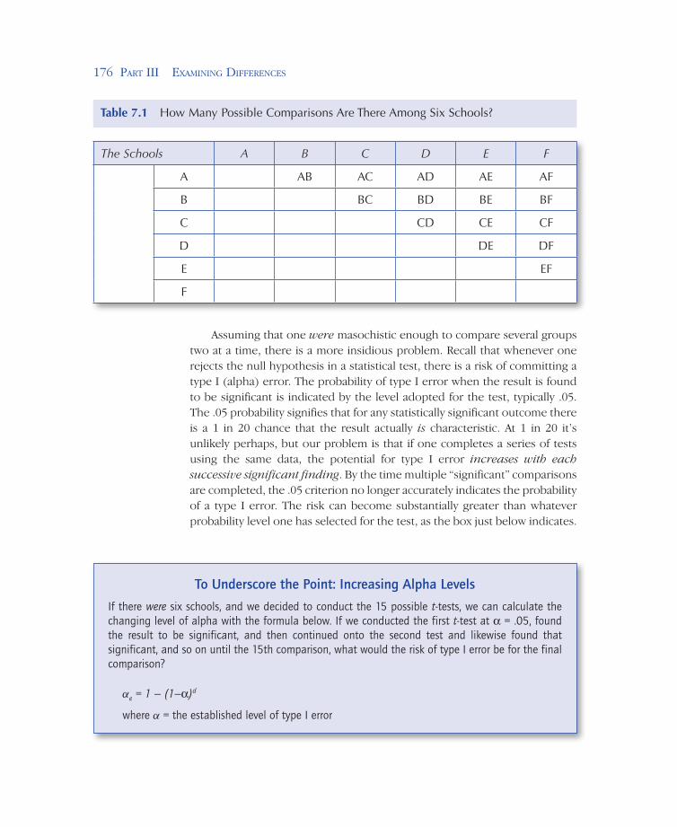
Extending this to more than three groups will reveal one of the problems with this approach. Calculating all possible comparisons with three schools is one thing, but it becomes unmanageable with large numbers of groups. What if there were six schools? Table 7.1 provides a matrix indicating all possible comparisons for six groups. Completing three independent t-tests probably isn’t an inordinate amount of work, but completing 15 tests (the number of groups times the number of groups minus 1, divided by 2) starts to look more than a little tedious, even with computer help!


Assuming that one were masochistic enough to compare several groups two at a time, there is a more insidious problem. Recall that whenever one rejects the null hypothesis in a statistical test, there is a risk of committing a type I (alpha) error. The probability of type I error when the result is found to be significant is indicated by the level adopted for the test, typically .05. The .05 probability signifies that for any statistically significant outcome there is a 1 in 20 chance that the result actually is characteristic. At 1 in 20 it’s unlikely perhaps, but our problem is that if one completes a series of tests using the same data, the potential for type I error increases with each successive significant finding. By the time multiple “significant” comparisons are completed, the .05 criterion no longer accurately indicates the probability of a type I error. The risk can become substantially greater than whatever probability level one has selected for the test, as the box just below indicates.

Table 7.1 How Many Possible Comparisons Are There Among Six Schools?

The Schools A B C D E F

A AB AC AD AE AF

B BC BD BE BF

C CD CE CF

D DE DF

E EF

F

To Underscore the Point: Increasing Alpha Levels

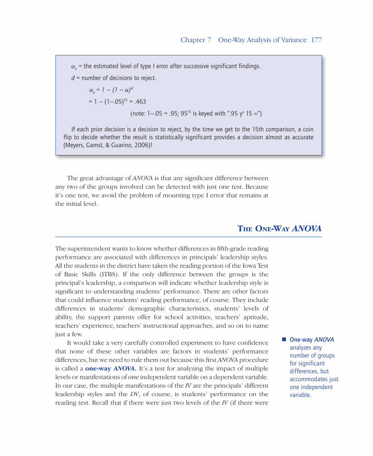
If there were six schools, and we decided to conduct the 15 possible t-tests, we can calculate the changing level of alpha with the formula below. If we conducted the first t-test at a = .05, found the result to be significant, and then continued onto the second test and likewise found that significant, and so on until the 15th comparison, what would the risk of type I error be for the final comparison?

αe = 1 − (1−a)d

where α = the established level of type I error


The great advantage of ANOVA is that any significant difference between any two of the groups involved can be detected with just one test. Because it’s one test, we avoid the problem of mounting type I error that remains at the initial level.

the One-Way ANOVA

The superintendent wants to know whether differences in fifth-grade reading performance are associated with differences in principals’ leadership styles. All the students in the district have taken the reading portion of the Iowa Test of Basic Skills (ITBS). If the only difference between the groups is the principal’s leadership, a comparison will indicate whether leadership style is significant to understanding students’ performance. There are other factors that could influence students’ reading performance, of course. They include differences in students’ demographic characteristics, students’ levels of ability, the support parents offer for school activities, teachers’ aptitude, teachers’ experience, teachers’ instructional approaches, and so on to name just a few.

It would take a very carefully controlled experiment to have confidence that none of these other variables are factors in students’ performance differences, but we need to rule them out because this first ANOVA procedure is called a one-way ANOVA. It’s a test for analyzing the impact of multiple levels or manifestations of one independent variable on a dependent variable. In our case, the multiple manifestations of the IV are the principals’ different leadership styles and the DV, of course, is students’ performance on the reading test. Recall that if there were just two levels of the IV (if there were

One-way ANOVA analyzes any number of groups for significant differences, but accommodates just one independent variable.

αe = the estimated level of type I error after successive significant findings.

d = number of decisions to reject.

αe = 1 − (1 − α)d

= 1 − (1−.05)15 = .463

(note: 1−.05 = .95; 9515 is keyed with “.95 yx 15 =”)

If each prior decision is a decision to reject, by the time we get to the 15th comparison, a coin flip to decide whether the result is statistically significant provides a decision almost as accurate (Meyers, Gamst, & Guarino, 2006)!


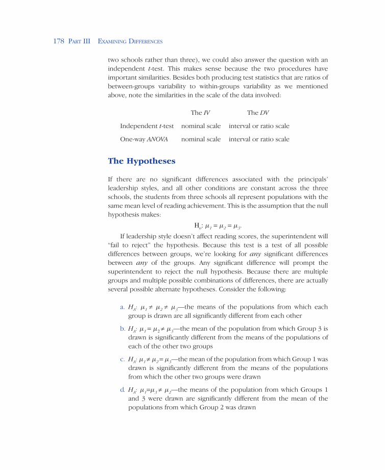
two schools rather than three), we could also answer the question with an independent t-test. This makes sense because the two procedures have important similarities. Besides both producing test statistics that are ratios of between-groups variability to within-groups variability as we mentioned above, note the similarities in the scale of the data involved:

The IV The DV

Independent t-test nominal scale interval or ratio scale

One-way ANOVA nominal scale interval or ratio scale

The Hypotheses

If there are no significant differences associated with the principals’ leadership styles, and all other conditions are constant across the three schools, the students from three schools all represent populations with the same mean level of reading achievement. This is the assumption that the null hypothesis makes:

Ho: µ1 = µ2 = µ3.

If leadership style doesn’t affect reading scores, the superintendent will “fail to reject” the hypothesis. Because this test is a test of all possible differences between groups, we’re looking for any significant differences between any of the groups. Any significant difference will prompt the superintendent to reject the null hypothesis. Because there are multiple groups and multiple possible combinations of differences, there are actually several possible alternate hypotheses. Consider the following:

a. HA: µ1 ≠ µ2 ≠ µ3—the means of the populations from which each group is drawn are all significantly different from each other

b. HA: µ1 = µ2 ≠ µ3—the mean of the population from which Group 3 is drawn is significantly different from the means of the populations of each of the other two groups

c. HA: µ1 ≠ µ2 = µ3—the mean of the population from which Group 1 was drawn is significantly different from the means of the populations from which the other two groups were drawn

d. HA: µ1=µ3 ≠ µ2—the means of the population from which Groups 1 and 3 were drawn are significantly different from the mean of the populations from which Group 2 was drawn


Perhaps prior research indicates that the students at the laissez-faire principal’s school (those at MacArthur School, No. 3) will perform differently than students at the other two schools. If that’s the hypothesis being tested, “b” is the alternate hypothesis. Ordinarily, however, the question is just whether there is a significant difference anywhere, so rather than listing all alternatives, something that gets messy with multiple groups, the alternate hypothesis is just a general:

HA: not so

This abbreviated alternate hypothesis just indicates that all groups do not represent populations with the same mean; that somewhere there’s a difference.

In the event that all groups don’t belong to populations with the same means and we reject Ho, there’s a problem we didn’t have with the t-test. The ANOVA test won’t indicate which group is significantly different from which, or whether all are different from each other, only that somewhere there’s a significant difference. We’ll tackle that problem later in the chapter with what are called post-hoc tests.

The Sources of Variance

Conceptually at least, much of what Fisher did was not entirely novel. We keep noting that in the independent t-test, Gosset examined the variability between groups (M1 − M2 , the numerator in the t ratio) and within groups (the standard error of the difference SEd, the denominator in the t-ratio) and there are corollaries in ANOVA. But rather than using the variance statistics used in the t-tests, the estimated standard error of the mean (SEM) and the standard error of the difference (SEd), Fisher used the sum of squares (SS) to measure data variability. Like any of the other measures of data variability, the sum of squares indicates how much scores tend to vary from a mean, and also like the others, the minimum possible SS value is 0; there’s no such thing as negative variance.

The Total Sum of Squares

Analysis of variance involves a number of group means. Besides the means of each group, M1, M2, and so on we will need a mean for all of the data. It’s the sum of all the scores in all of the groups divided by the total

Sum of squares values are the sum of the squared deviations of individual scores from a mean.


number of all subjects, N. We’ll call this mean the grand mean (MG). Recall from Chapter 2 that part of what we did to calculate variance and standard deviation statistics was to subtract the mean of the group from each individual score, square the differences, and then sum the squared differences.

If one were to follow that same procedure with the MG, subtracting it from each score in all of the groups, the result is a measure of data variability for all the groups together. Based on the sum of the squared deviations of all the individual scores from the grand mean, it’s called a sum of squares value. In this case, because it’s based on data from all the individuals in all of the groups it’s called the sum of squares total, SStot and it’s an important component of analysis of variance. The formula for SStot is as follows:

SStot = Σ(x − MG)2 7.1

Where,

SStot = the total sum of squares

x = each individual score

MG = the mean of all scores, “the grand mean”

Σ(x − MG)2= the sum of the squared differences between each individual score in each group and the grand mean

To repeat the steps for calculating SStot:

1. Calculate the mean of all scores from all groups combined (MG)

2. Subtract MG from each individual score

3. Square each of the differences

4. Sum the squared differences to get SSt

There are other ways to calculate SStot, as well as the other SS values that are coming up, but they all result in the same values. When there are large data sets and a good deal of longhand calculating, some authors recommend the use of what are called “calculation formulae” (see, for example, Sprinthall, 2007). They make the work less tedious, but sometimes the logic isn’t very clear. Since using the computer is likely how you’ll do most of your ANOVA work anyway, we’ll take a conceptual approach so that the logic behind these SS statistics makes more intuitive sense.

Remember that the designation “SStot” indicates that this statistic includes all variability from all sources. The “analysis” in analysis of variance is the


business of deriving and comparing the variance between individual groups and the grand mean MG, and the variability that occurs within the individual groups. The ANOVA test statistic, F, is going to be the ratio of the between-groups variability to the within-groups variability.

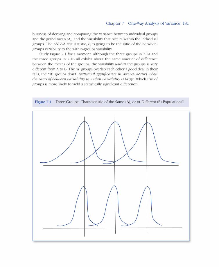
Study Figure 7.1 for a moment. Although the three groups in 7.1A and the three groups in 7.1B all exhibit about the same amount of difference between the means of the groups, the variability within the groups is very different from A to B. The “A” groups overlap each other a good deal in their tails; the “B” groups don’t. Statistical significance in ANOVA occurs when the ratio of between variability to within variability is large. Which trio of groups is more likely to yield a statistically significant difference?

Figure 7.1 Three Groups: Characteristic of the Same (A), or of Different (B) Populations?


With the same between variability in both, but much more within variability in the “A” groups, can you see that the “B” groups are going to yield a much larger ratio of between-to-within variability? The within variability is likely going to overwhelm the between variability in the “A” groups. Although we’re calculating variability differently, it is still the ratio of between groups variability to within groups variability that we’re interested in, just as it was with the independent t-test in Chapter 6.

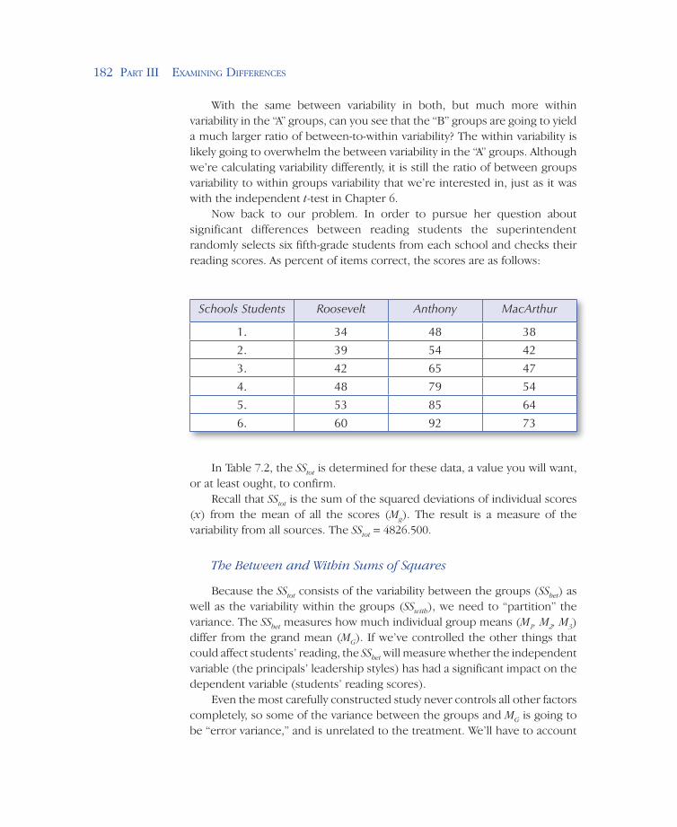
Now back to our problem. In order to pursue her question about significant differences between reading students the superintendent randomly selects six fifth-grade students from each school and checks their reading scores. As percent of items correct, the scores are as follows:

Schools Students Roosevelt Anthony MacArthur

1. 34 48 38

2. 39 54 42

3. 42 65 47

4. 48 79 54

5. 53 85 64

6. 60 92 73

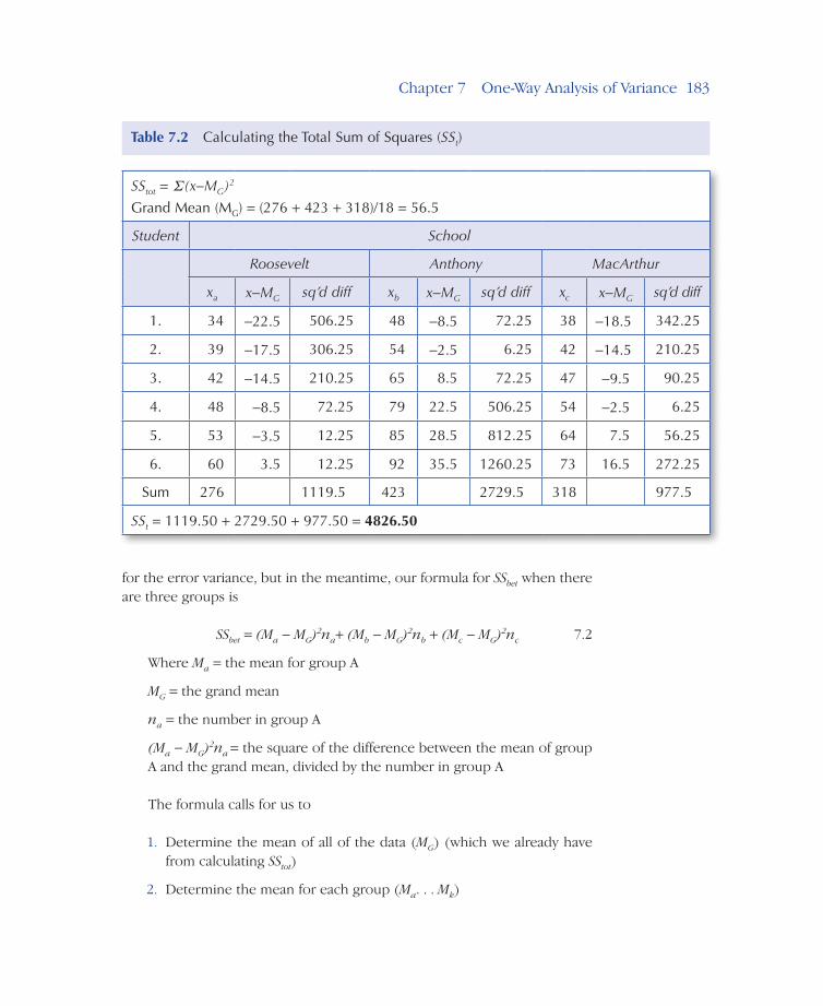
In Table 7.2, the SStot is determined for these data, a value you will want, or at least ought, to confirm.

Recall that SStot is the sum of the squared deviations of individual scores (x) from the mean of all the scores (Mg). The result is a measure of the variability from all sources. The SStot = 4826.500.

The Between and Within Sums of Squares

Because the SStot consists of the variability between the groups (SSbet) as well as the variability within the groups (SSwith), we need to “partition” the variance. The SSbet measures how much individual group means (M1, M2, M3) differ from the grand mean (MG). If we’ve controlled the other things that could affect students’ reading, the SSbet will measure whether the independent variable (the principals’ leadership styles) has had a significant impact on the dependent variable (students’ reading scores).

Even the most carefully constructed study never controls all other factors completely, so some of the variance between the groups and MG is going to be “error variance,” and is unrelated to the treatment. We’ll have to account


for the error variance, but in the meantime, our formula for SSbet when there are three groups is

SSbet = (Ma − MG)2na+ (Mb − MG)2nb + (Mc − MG)2nc 7.2

Where Ma = the mean for group A

MG = the grand mean

na = the number in group A

(Ma − MG)2na = the square of the difference between the mean of group A and the grand mean, divided by the number in group A

The formula calls for us to

1. Determine the mean of all of the data (MG) (which we already have from calculating SStot)

2. Determine the mean for each group (Ma. . . Mk)

SStot = Σ(x−MG)2

Grand Mean (MG) = (276 + 423 + 318)/18 = 56.5

Student School

Roosevelt Anthony MacArthur

xa x−MG sq’d diff xb x−MG sq’d diff xc x−MG sq’d diff

1. 34 −22.5 506.25 48 −8.5 72.25 38 −18.5 342.25

2. 39 −17.5 306.25 54 −2.5 6.25 42 −14.5 210.25

3. 42 −14.5 210.25 65 8.5 72.25 47 −9.5 90.25

4. 48 −8.5 72.25 79 22.5 506.25 54 −2.5 6.25

5. 53 −3.5 12.25 85 28.5 812.25 64 7.5 56.25

6. 60 3.5 12.25 92 35.5 1260.25 73 16.5 272.25

Sum 276 1119.5 423 2729.5 318 977.5

SSt = 1119.50 + 2729.50 + 977.50 = 4826.50

Table 7.2 Calculating the Total Sum of Squares (SSt)


3. Subtract MG from each group mean

4. Square the difference

5. Adjust for sample size by multiplying the squared difference by the number in each group

For the students from the three schools, the group means are

• Roosevelt Ma = 46.0 • Anthony Mb = 70.50 • MacArthur Mc = 53.0

For all the data together the mean (MG) = 56.5 (Table 7.2). Since n = 6 in each group, we calculate SSbet as follows:

SSbet = (46 − 56.5)26 + (70.50 − 56.5)26 + (53.0 − 56.50)26 = 1911.00

The SSw, conversely, is a measure of how much data vary within the groups. Because they differ individually, even students from the same school don’t all respond the same way to a stimulus (the principal’s leadership). Unavoidably, some of this variability shows up in SSbet, but in SSw it’s all differences within groups. The evidence for it is the differences there are between the scores of individuals in the same group. We’ll measure SSw by comparing scores in each group to their group means. Consider Formula 7.3:

SSwith = Σ (xa − Ma)2 + Σ (xb − Mb)2 + Σ (xc − Mc)

2 7.3

This formula indicates that there are three groups, a, b, and c (representing the three schools), and we understand the terms as follows:

SSwith = the sum of squares within and

Σ = summation, or sum of xa = for each score in group “a”

Ma = the mean of the scores in group “a”

Σ (xa− Ma)2= the sum of the squared differences between individuals in group a (xa) and the mean of group a

To calculate SSw

1. Determine the mean of the scores from group “a” (Ma)

2. Subtract Ma from each score in group “a”


3. Square each difference value

4. Sum the squared differences for the group

5. Repeat Steps 1–4 for each of the other groups

6. Sum the results across the groups

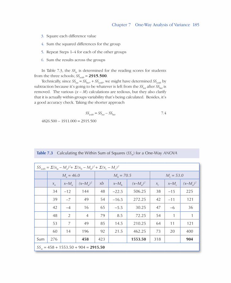
In Table 7.3, the SSw is determined for the reading scores for students from the three schools; SSwith = 2915.500.

Technically, since SStot = SSbet, + SSwith, we might have determined SSwith by subtraction because it’s going to be whatever is left from the SStot after SSbet is removed. The various (x – M) calculations are tedious, but they also clarify that it is actually within-groups variability that’s being calculated. Besides, it’s a good accuracy check. Taking the shorter approach

SSwith = SStot – SSbet 7.4

4826.500 – 1911.000 = 2915.500

SSwith = Σ(xa − Ma)2+ Σ(xb − Mb)

2 + Σ(xc − Mc)2

Ma = 46.0 Mb = 70.5 Mc = 53.0

xa x−Ma (x−Ma)2 xb x−Mb (x−Ma)

2 xc x−Mc (x−Ma)2

34 −12 144 48 −22.5 506.25 38 −15 225

39 −7 49 54 −16.5 272.25 42 −11 121

42 −4 16 65 −5.5 30.25 47 −6 36

48 2 4 79 8.5 72.25 54 1 1

53 7 49 85 14.5 210.25 64 11 121

60 14 196 92 21.5 462.25 73 20 400

Sum 276 458 423 1553.50 318 904

SSw = 458 + 1553.50 + 904 = 2915.50

Table 3.1 The Percentage of Scores in a Particular StanineTable 7.3 Calculating the Within Sum of Squares (SSw) for a One-Way ANOVA


Subtraction is certainly the easier approach, but if we derive SSwith this way and there is an error with the SSbet calculation, it’s just perpetuated with SSwith. If the SSbet and SSwith are calculated independently, we can always dou-ble-check when finished to make sure they sum to SStot.

Interpreting the Variability Measures

So what do these SS values mean? Although sums of squares are variability measures like standard deviation and variances, a difference is that sums of squares values increase as the number of scores increases. Recall that standard deviation and variance measures values tend to shrink with additional data because scores near the mean of the distribution are more common than scores in the tails. Sums of squares don’t shrink. Adding scores means more squared differences to add, which will always result in larger values.

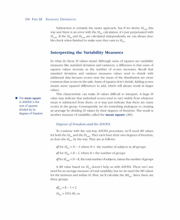
This characteristic can make SS values difficult to interpret. A large SS value may indicate that individual scores tend to vary widely from whatever mean is subtracted from them, or it may just indicate that there are many scores in the group. Consequently, we do something analogous to creating an average by dividing SS values by their degrees of freedom. The result is another measure of variability called the mean square (MS).

Degrees of Freedom and the ANOVA

To continue with the one-way ANOVA procedure, we’ll need MS values for both the SSbet and the SSwith. They each have their own degrees of freedom, as does the SStot, by the way. They are as follows:

df for SStot = N − 1 where N = the number of subjects in all groups

df for SSbet = k − l, where k = the number of groups

df for SSwith = N − K, the total number of subjects, minus the number of groups

A MS value based on SStot doesn’t help us with ANOVA. There isn’t any need for an average measure of total variability, but we do need the MS values for the between and within SS. First, we’ll calculate the MSbet. Since there are three groups

dfbet = k – 1 = 2

SSbet = 1911.00, so

The mean square in ANOVA is the sum of squares divided by its degrees of freedom.


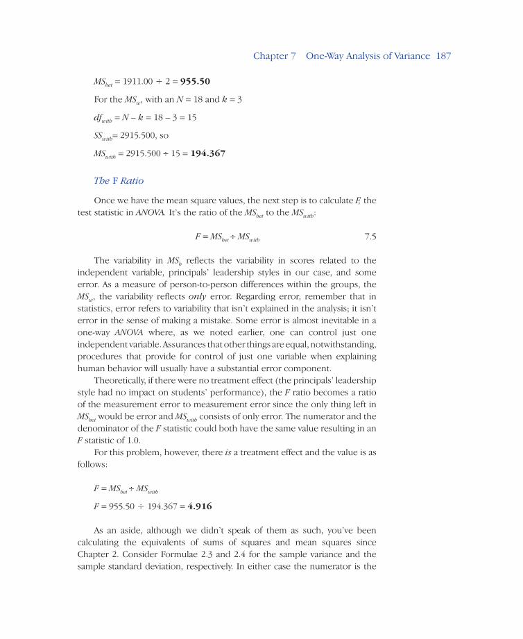
MSbet = 1911.00 ÷ 2 = 955.50

For the MSw, with an N = 18 and k = 3

dfwith = N – k = 18 – 3 = 15

SSwith= 2915.500, so

MSwith = 2915.500 ÷ 15 = 194.367

The F Ratio

Once we have the mean square values, the next step is to calculate F, the test statistic in ANOVA. It’s the ratio of the MSbet to the MSwith:

F = MSbet ÷ MSwith 7.5

The variability in MSb reflects the variability in scores related to the independent variable, principals’ leadership styles in our case, and some error. As a measure of person-to-person differences within the groups, the MSw, the variability reflects only error. Regarding error, remember that in statistics, error refers to variability that isn’t explained in the analysis; it isn’t error in the sense of making a mistake. Some error is almost inevitable in a one-way ANOVA where, as we noted earlier, one can control just one independent variable. Assurances that other things are equal, notwithstanding, procedures that provide for control of just one variable when explaining human behavior will usually have a substantial error component.

Theoretically, if there were no treatment effect (the principals’ leadership style had no impact on students’ performance), the F ratio becomes a ratio of the measurement error to measurement error since the only thing left in MSbet would be error and MSwith consists of only error. The numerator and the denominator of the F statistic could both have the same value resulting in an F statistic of 1.0.

For this problem, however, there is a treatment effect and the value is as follows:

F = MSbet ÷ MSwith

F = 955.50 ÷ 194.367 = 4.916

As an aside, although we didn’t speak of them as such, you’ve been calculating the equivalents of sums of squares and mean squares since Chapter 2. Consider Formulae 2.3 and 2.4 for the sample variance and the sample standard deviation, respectively. In either case the numerator is the


sum of the squared deviations of individual scores from their mean, Σ(x – M)2. That makes those numerators SS values. The denominator was n − 1, the degrees of freedom value. Dividing the SS value by their df produces what we have here called the mean square!

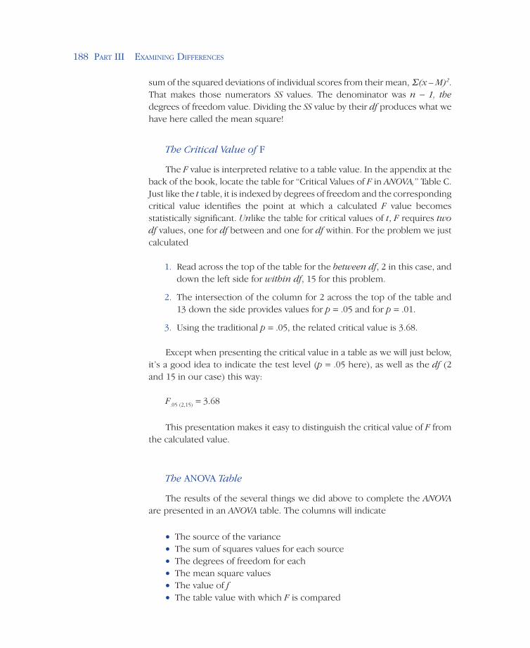
The Critical Value of F

The F value is interpreted relative to a table value. In the appendix at the back of the book, locate the table for “Critical Values of F in ANOVA,” Table C. Just like the t table, it is indexed by degrees of freedom and the corresponding critical value identifies the point at which a calculated F value becomes statistically significant. Unlike the table for critical values of t, F requires two df values, one for df between and one for df within. For the problem we just calculated

1. Read across the top of the table for the between df, 2 in this case, and down the left side for within df, 15 for this problem.

2. The intersection of the column for 2 across the top of the table and 13 down the side provides values for p = .05 and for p = .01.

3. Using the traditional p = .05, the related critical value is 3.68.

Except when presenting the critical value in a table as we will just below, it’s a good idea to indicate the test level (p = .05 here), as well as the df (2 and 15 in our case) this way:

F.05 (2,15) = 3.68

This presentation makes it easy to distinguish the critical value of F from the calculated value.

The ANOVA Table

The results of the several things we did above to complete the ANOVA are presented in an ANOVA table. The columns will indicate

• The source of the variance • The sum of squares values for each source • The degrees of freedom for each • The mean square values • The value of f • The table value with which F is compared


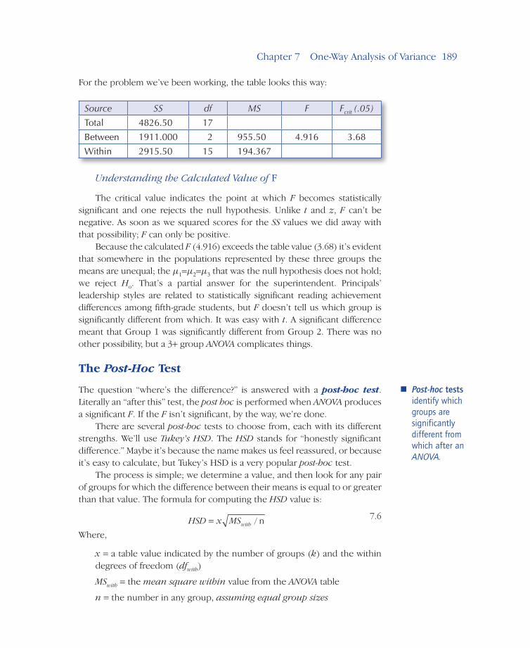
For the problem we’ve been working, the table looks this way:

Source SS df MS F Fcrit (.05)

Total 4826.50 17

Between 1911.000 2 955.50 4.916 3.68

Within 2915.50 15 194.367

Understanding the Calculated Value of F

The critical value indicates the point at which F becomes statistically significant and one rejects the null hypothesis. Unlike t and z, F can’t be negative. As soon as we squared scores for the SS values we did away with that possibility; F can only be positive.

Because the calculated F (4.916) exceeds the table value (3.68) it’s evident that somewhere in the populations represented by these three groups the means are unequal; the µ1=µ2=µ3 that was the null hypothesis does not hold; we reject Ho. That’s a partial answer for the superintendent. Principals’ leadership styles are related to statistically significant reading achievement differences among fifth-grade students, but F doesn’t tell us which group is significantly different from which. It was easy with t. A significant difference meant that Group 1 was significantly different from Group 2. There was no other possibility, but a 3+ group ANOVA complicates things.

The Post-Hoc Test

The question “where’s the difference?” is answered with a post-hoc test. Literally an “after this” test, the post hoc is performed when ANOVA produces a significant F. If the F isn’t significant, by the way, we’re done.

There are several post-hoc tests to choose from, each with its different strengths. We’ll use Tukey’s HSD. The HSD stands for “honestly significant difference.” Maybe it’s because the name makes us feel reassured, or because it’s easy to calculate, but Tukey’s HSD is a very popular post-hoc test.

The process is simple; we determine a value, and then look for any pair of groups for which the difference between their means is equal to or greater than that value. The formula for computing the HSD value is:

HSD x MSwith= / n 7.6

Where,

x = a table value indicated by the number of groups (k) and the within degrees of freedom (dfwith)

MSwith = the mean square within value from the ANOVA table

n = the number in any group, assuming equal group sizes

Post-hoc tests identify which groups are significantly different from which after an ANOVA.


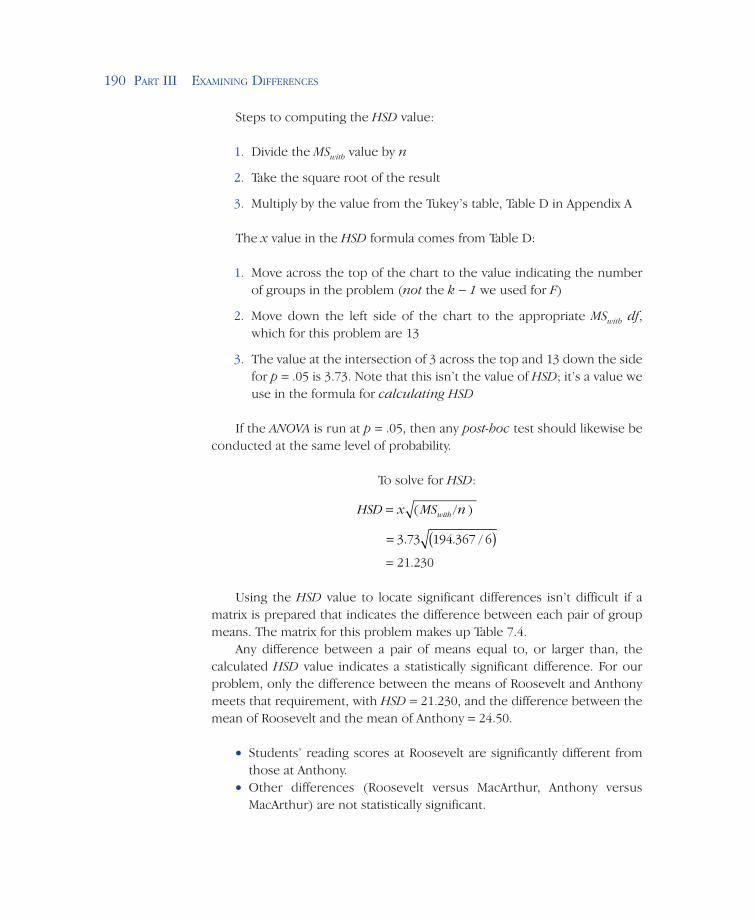
Steps to computing the HSD value:

1. Divide the MSwith value by n

2. Take the square root of the result

3. Multiply by the value from the Tukey’s table, Table D in Appendix A

The x value in the HSD formula comes from Table D:

1. Move across the top of the chart to the value indicating the number of groups in the problem (not the k − 1 we used for F)

2. Move down the left side of the chart to the appropriate MSwith df, which for this problem are 13

3. The value at the intersection of 3 across the top and 13 down the side for p = .05 is 3.73. Note that this isn’t the value of HSD; it’s a value we use in the formula for calculating HSD

If the ANOVA is run at p = .05, then any post-hoc test should likewise be conducted at the same level of probability.

To solve for HSD:

HSD x MS nwith= ( / )

= ( )3.73 194 367 6. /

= 21.230

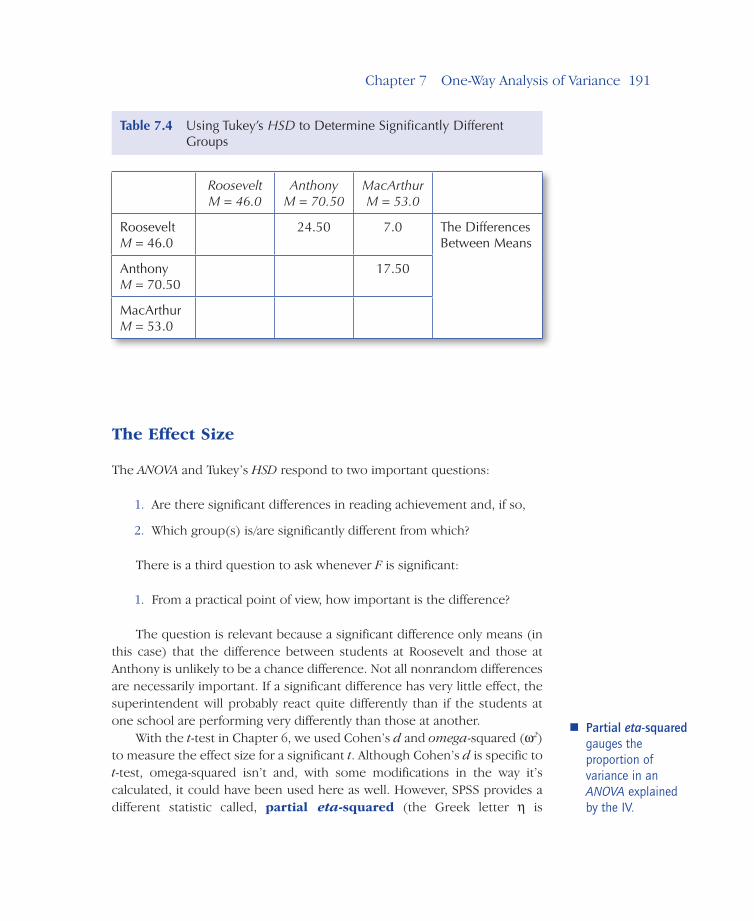
Using the HSD value to locate significant differences isn’t difficult if a matrix is prepared that indicates the difference between each pair of group means. The matrix for this problem makes up Table 7.4.

Any difference between a pair of means equal to, or larger than, the calculated HSD value indicates a statistically significant difference. For our problem, only the difference between the means of Roosevelt and Anthony meets that requirement, with HSD = 21.230, and the difference between the mean of Roosevelt and the mean of Anthony = 24.50.

• Students’ reading scores at Roosevelt are significantly different from those at Anthony.

• Other differences (Roosevelt versus MacArthur, Anthony versus MacArthur) are not statistically significant.


The Effect Size

The ANOVA and Tukey’s HSD respond to two important questions:

1. Are there significant differences in reading achievement and, if so,

2. Which group(s) is/are significantly different from which?

There is a third question to ask whenever F is significant:

1. From a practical point of view, how important is the difference?

The question is relevant because a significant difference only means (in this case) that the difference between students at Roosevelt and those at Anthony is unlikely to be a chance difference. Not all nonrandom differences are necessarily important. If a significant difference has very little effect, the superintendent will probably react quite differently than if the students at one school are performing very differently than those at another.

With the t-test in Chapter 6, we used Cohen’s d and omega-squared (w2) to measure the effect size for a significant t. Although Cohen’s d is specific to t-test, omega-squared isn’t and, with some modifications in the way it’s calculated, it could have been used here as well. However, SPSS provides a different statistic called, partial eta-squared (the Greek letter h is

Partial eta-squared gauges the proportion of variance in an ANOVA explained by the IV.

Roosevelt M = 46.0

AnthonyM = 70.50

MacArthurM = 53.0

RooseveltM = 46.0

24.50 7.0 The Differences Between Means

AnthonyM = 70.50

17.50

MacArthurM = 53.0

Table 7.4 Using Tukey’s HSD to Determine Significantly Different Groups


pronounced like “ate a”), so we’ll use that instead. It answers the same question that omega-squared answered for t-test:

How much of the variability in the DV (reading scores) can be attributed to the IV (the principal’s leadership style)?

The formula for partial eta-squared is

η p

bet

bet with

SS

SS SS2 =

+ 7.7

This is an easy calculation since the sums of squares values needed are already available from the ANOVA table. For our data the value of partial eta-squared is:

ηp2 = 1911.00/(1911.00 + 2915.50)

= .396

About 40% (the hp2 value multiplied by 100 and rounded) of the group

differences in reading scores can be explained by the principal’s leadership style. This eta-squared value is probably unrealistically high, of course. Learners and learning environments are far too complex to make it likely that one variable will explain so much of the variance in reading achievement. Anyway, it’s the calculation and interpretation we’re interested in just now, not the validity as such.

Requirements for the One-Way ANOVA

1. Because it’s a “one-way” ANOVA, there can be just one IV. That varia-ble may have any number of levels or expressions more than one, but there can be just one variable whether it’s the type of instruction, the school with which the group is associated, the level of drug the patient is given, or whatever.

2. The independent variable data either must be in categorical form (nominal scale) to begin with, or reduced to categorical form.

3. The dependent variable data must be at least interval scale.

4. The groups or categories must be independent. Subjects cannot belong to more than one group in this form of ANOVA.


5. There must be the same homogeneity of variance that t-test requires—all groups must be distributed similarly.

6. Finally, it is assumed that the population from which the subjects are drawn is normally distributed.

Happily, ANOVA is pretty forgiving (the statistical lingo is “robust”) when homogeneity of variance and normality assumptions are violated, particularly when the groups are relatively large. So unless there is a fairly obvious problem with the way the data are distributed, or with their normality, one needn’t worry too much about these particular requirements.

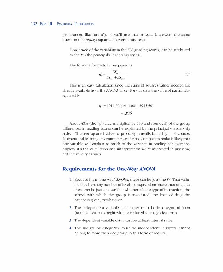
“Rather than a play-off to determine the championship, we suggest a post-hoc test conducted at p = .05.”

SOU

RC

E: C

reat

ed b

y Su

zann

a N

iels

on.


lOOking at sPss OutPut

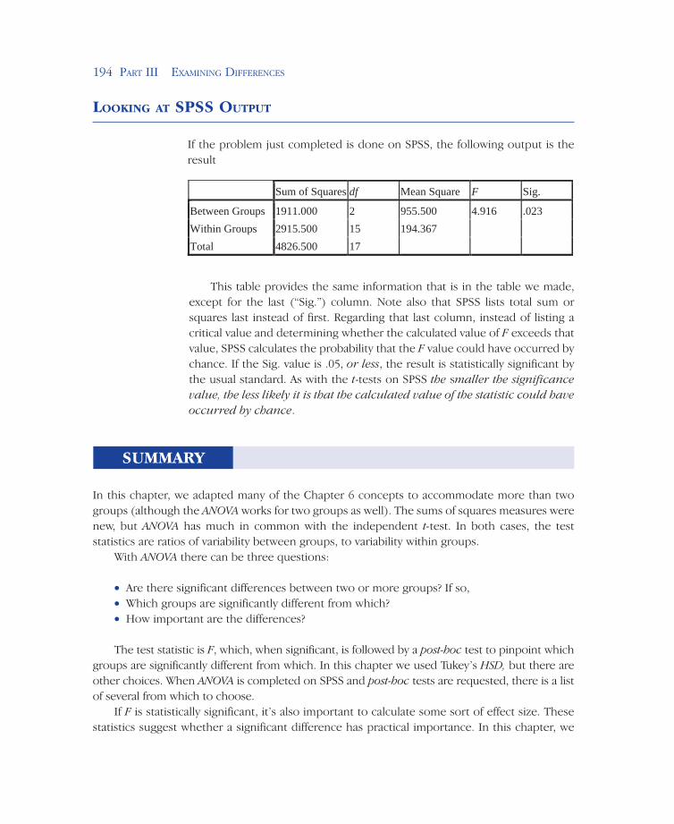
If the problem just completed is done on SPSS, the following output is the result

Sum of Squares df Mean Square F Sig.

Between Groups 1911.000 2 955.500 4.916 .023Within Groups 2915.500 15 194.367Total 4826.500 17

This table provides the same information that is in the table we made, except for the last (“Sig.”) column. Note also that SPSS lists total sum or squares last instead of first. Regarding that last column, instead of listing a critical value and determining whether the calculated value of F exceeds that value, SPSS calculates the probability that the F value could have occurred by chance. If the Sig. value is .05, or less, the result is statistically significant by the usual standard. As with the t-tests on SPSS the smaller the significance value, the less likely it is that the calculated value of the statistic could have occurred by chance.

SUMMARY

In this chapter, we adapted many of the Chapter 6 concepts to accommodate more than two groups (although the ANOVA works for two groups as well). The sums of squares measures were new, but ANOVA has much in common with the independent t-test. In both cases, the test statistics are ratios of variability between groups, to variability within groups.

With ANOVA there can be three questions:

• Are there significant differences between two or more groups? If so, • Which groups are significantly different from which? • How important are the differences?

The test statistic is F, which, when significant, is followed by a post-hoc test to pinpoint which groups are significantly different from which. In this chapter we used Tukey’s HSD, but there are other choices. When ANOVA is completed on SPSS and post-hoc tests are requested, there is a list of several from which to choose.

If F is statistically significant, it’s also important to calculate some sort of effect size. These statistics suggest whether a significant difference has practical importance. In this chapter, we


used partial eta-squared. When the F isn’t statistically significant, by the way, both the post-hoc test and the effect size calculation are irrelevant since any variation between the characteristics of the groups is just random.

The one-way ANOVA is an important advance in statistical analysis, but very few of the problems instructors, counselors, or administrators are interested in lend themselves to single-variable explanations. Such approaches leave too much of the variance uncontrolled. The factorial ANOVA discussion that is Chapter 8 will allow us to include additional independent variables that are important to the analysis and so limit the variability that otherwise becomes error variance.

This analysis of variance chapter is probably the single most involved chapter in the book, but here you are and you ought to be reassured for having navigated it. Well done! Having triumphed over ANOVA, do the end-of-chapter problems while the concepts are fresh and then restudy the chapter to be sure that you can explain what you’ve done. The next chapter on factorial ANOVA builds squarely on this material.

EXERCISES

1. A group of learners is assigned a task that they may discontinue at any time. Using the num-ber of minutes they remain on task as a measure of motive strength, we have the following measures: 1.0, 1.5, 1.5, 2.25. 3.0, 5.0 6.25. What is the sum of squares total for these data?

2. In a one-way ANOVA, identify the following:

a. The measure of all variance from all sourcesb. The measure that indicates the average impact of the IVc. The average measure of uncontrolled variance

3. We have the following data on number of units for two groups of university students signing up for classes. One group is international students, and the other is from the local area. Treating the problem as an ANOVA in spite of the fact that there are just two groups, is there a significant difference in the number of units for which students in each group register?

a. International Students: 12, 14, 16, 16, 17, 18, 18 18b. Domestic Students: 12, 12, 12, 14, 14, 14, 14, 16

4. Complete an independent t-test for the data in problem 3. If you square the value of t (t2), what’s its relationship to the F value in problem 3?

5. Even should the F be significant, why is a post-hoc test unnecessary in a problem like 3?

6. What’s the point of calcuating hp2?

7. Three groups of students involved in the same curriculum are obliged to study for 15 min-utes, 30 minutes, or 90 minutes a night for 8 weeks before taking a mathematics test. Their scores are as follows:

15 minutes: 43, 39, 55, 56, 7330 minutes: 55, 58, 66, 79, 8290 minutes: 61, 66, 85, 86, 91


a. Are the differences statistically significant?b. If F is significant, which group(s) is(are) significantly different from which?c. How much of the difference in mathematics performance can be explained by how long

students study?

8. In item 7, what is the independent variable?

a. What is the data scale of the independent variable?b. What is the dependent variable?c. What is the data scale of the dependent variable?

9. A particular ANOVA problem involves four groups with 10 in each.

SSbet = 24.0 SSwith = 72What’s the value of F?Is F statistically significant?

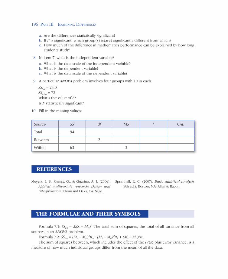
10. Fill in the missing values:

Source SS df MS F Crit.

Total 94

Between 2

Within 63 3

REFERENCES

Meyers, L. S., Gamst, G., & Guarino, A. J. (2006). Applied multivariate research: Design and interpretation. Thousand Oaks, CA: Sage.

Sprinthall, R. C. (2007). Basic statistical analysis (8th ed.). Boston, MA: Allyn & Bacon.

THE FORMULAE AND THEIR SYMBOLS

Formula 7.1: SStot = Σ(x − MG)2 The total sum of squares, the total of all variance from all sources in an ANOVA problem.

Formula 7.2: SSbet = (Ma − MG)2na+ (Mb − MG)2nb + (Mc − MG)2nc The sum of squares between, which includes the effect of the IV(s) plus error variance, is a

measure of how much individual groups differ from the mean of all the data.


Formula 7.3: SSwith = Σ (xa − Ma)2 + Σ (xb − Mb)2 + Σ (xc − Mc )2

The sum of squares within is a measure of how much individuals within a group differ when exposed to the same level of the IV(s). It’s a measure of error variance.

Formula 7.4: SSwith = SStot – SSbet An alternate method for determining SSw, it indicates that if the SSbet is subtracted from SSt, what is left is SSw.

Formula 7.5: F = MSbet ÷ MSwith. The F is the test statistic in analysis of variance. It’s a ratio of treatment effect plus error variance, to just error vari-ance.

Formula 7.6: HSD = x MS nw( / ) Tukey’s HSD is a post-hoc test used to determine which groups in an ANOVA are significantly different from which.

Formula 7.7: hp2 = SSbet /(SSbet + SSw) Partial eta-squared is an estimate of

effect size. It suggests the proportion of variance explained by the particular component. In this configuration it’s the variability between groups.

STUDENT STUDY SITE

Visit the Student Study Site at www.sagepub.com/tanner for additional learning tools.

the problem: how to detect significant differences in more ... · one-way analysis of variance 173...

Documents