THE UNIVERSITY OF HONG KONGLIBRARIES

REVIEW OF NATURALTERRAIN LANDSLIDE

DEBRIS-RESISTINGBARRIER DESIGN

GEO REPORT No. 104

D.O.K. Lo

This report was originally produced in January 2000as GEO Special Project Report No. SPR1/2000

3e « <>,

t ? JUN 212

- 2 -

© The Government of the Hong Kong Special Administrative Region

First published, November 2000

Prepared by:

Geotechnical Engineering Office,Civil Engineering Department,Civil Engineering Building,101 Princess Margaret Road,Homantin, Kowloon,Hong Kong.

NO.

This publication is available from:

Government Publications Centre,Ground Floor, Low Block,Queensway Government Offices,66 Queensway,Hong Kong.

Overseas orders should be placed with:

Publications Sales Section,Information Services Department,Room 402,4th Floor, Murray Building,Garden Road, Central,Hong Kong.

Price in Hong Kong: HK$58Price overseas: US$11 (including surface postage)

An additional bank charge of HK$50 or US$6.50 is required per cheque made in currenciesother than Hong Kong dollars.

Cheques, bank drafts or money orders must be made payable toThe Government of the Hong Kong Special Administrative Region.

3 -

PREFACE

In keeping with our policy of releasing informationwhich may be of general interest to the geotechnical professionand the public, we make available selected internal reports in aseries of publications termed the GEO Report series, A chargeis made to cover the cost of printing.

The Geotechnical Engineering Office also publishesguidance documents as GEO Publications. These publicationsand the GEO Reports may be obtained from the Government'sInformation Services Department. Information on how topurchase these documents is given on the last page of thisreport.

R.K.S.ChanHead, Geotechnical Engineering Office

November 2000

- 4 -

FOREWORD

As part of the development of natural terrain landsliderisk management strategy for Hong Kong, the GeotechnicalEngineering Office is conducting a series of studies to developtechniques for quantifying natural terrain hazard and risk and toassess the range of practicable risk mitigation measures, so thata balanced and cost-effective strategy can be formulated.

This study examines the design of landslide debris-resisting barriers. The main aim is to identify methods that canproduce reasonable estimates of the debris mobility and debrisimpact loads for use in engineering design. Variousapproaches suggested in the literature for assessing the mobilityof debris and debris impact loads have been reviewed andevaluated in the light of laboratory and field measurements.Some suggestions are put forward to facilitate design. Giventhe developments in the subject, the suggestions are intended tobe interim. They will be reviewed and updated when new dataand results of further research become available.

This study was carried out by Dr D.O.K. Lo, under thesupervision of initially Mr K.K.S. Ho and later Mr W.K. Punand Mr Y.K. Shiu. Useful information has been provided byProf. Z. Kang and Mr S. Zhang of the Institute of MountainousEnvironment and Hazards, Chinese Academy of Sciences andMinistry of Water Conservation, Mr R. Du and Mr S. Wang ofthe Dongchuan Institute of Debris Flow Control, ChineseAcademy of Sciences, Mr B. Hosle of Fatzer AG, Switzerland,and Mr D.F. VanDine of VanDine Geological Engineering Ltd,Canada. Their assistance is gratefully acknowledged.

P.L.R. PangChief Geotechnical Engineer/Special Projects

5 -

ABSTRACT

The demand for land in the hilly terrain of Hong Kong means there is increasingpressure for developments to encroach onto the steeper parts of its natural terrain. Typicallymore than 300 natural terrain landslides occur in Hong Kong every year. The vast majority ofthese are shallow failures involving the top few metres of the ground surface and some maydevelop into channelised debris flows with long runout. Given the close proximity of some ofthe developments to natural hillsides, even a relatively small failure can potentially result inserious consequences.

Preventive works on the hillside can be extensive and prohibitively costly and landslidebarriers may prove to be a cost-effective solution in certain situations. This study examinessome salient aspects of the design of barriers for natural terrain landslides. Key data on someof the barriers constructed in Hong Kong are presented. Various approaches put forward inthe literature for evaluating the impact loads on barriers have been reviewed and thisillustrates, inter alia, the considerable scatter in the predictions as well as in some of thereported field measurements.

Based on the present state of knowledge, some suggestions are put forward to facilitatethe assessment of debris mobility and debris impact loads in the design of landslide debris-resisting barriers. Given the developments in the subject, the suggestions are intended to beinterim. They will be reviewed and updated when new data and results of further researchbecome available.

Further research is needed to gain a better fundamental understanding of the nature andmechanisms of natural hillside failures in Hong Kong and to improve the methods forassessment of debris mobility and debris impact loads under local conditions.

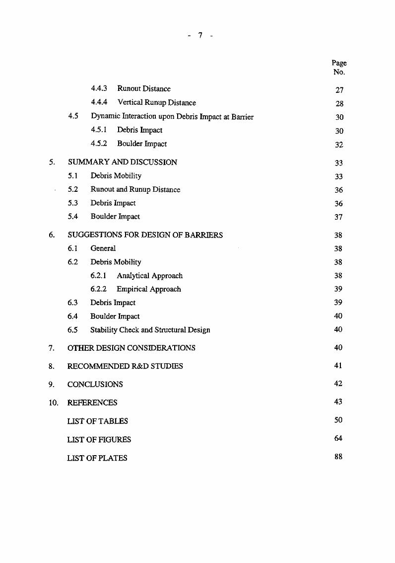
CONTENTS

PageNo.

^ Title Page 1

PREFACE 3

FOREWORD 4

ABSTRACT 5

CONTENTS 6

1. INTRODUCTION 8

1.1 General 8

1.2 Landslide Hazards and Zones 8

1.3 Mitigation Measures 8

2. TYPES OF BARRIERS 9

2.1 Overseas Practice 9

2.2 Local Practice 11

3. REVIEW OF LOCAL DESIGN CASES 11

3.1 Design Volume 11

3.2 Impact Loading 12

33 Debris Mobility 14

4. DESIGN METHODOLOGIES 14

4.1 General 14

4.2 Characterisation of Landslide Hazards 15

4.3 Characterisation of Design Events 16

4.3.1 General 16

4.3.2 Methods for Estimating Debris Flow Volumes 16

4.3.3 Peak Discharge of Debris Flows 19

4.3.4 Discussion 19

4.4 Characterisation of Debris Movement 20

4.4.1 General 20

4.4.2 Methods for Estimating Debris Velocity and Runout 21

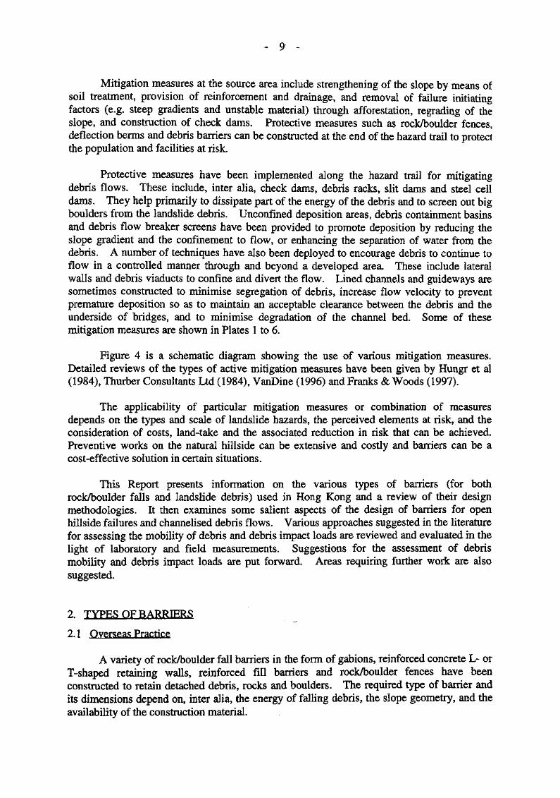
7 -

PageNo.

4.4.3 Runout Distance 27

4.4.4 Vertical Runup Distance 28

4.5 Dynamic Interaction upon Debris Impact at Barrier 30

4.5.1 Debris Impact 30

4.5.2 Boulder Impact 32

5. SUMMARY AND DISCUSSION 33

5.1 Debris Mobility 33

5.2 Runout and Runup Distance 36

5.3 Debris Impact 36

5.4 Boulder Impact 37

6. SUGGESTIONS FOR DESIGN OF BARRIERS 38

6.1 General 38

6.2 Debris Mobility 38

6.2.1 Analytical Approach 38

6.2.2 Empirical Approach 39

6.3 Debris Impact 39

6.4 Boulder Impact 40

6.5 Stability Check and Structural Design 40

7. OTHER DESIGN CONSIDERATIONS 40

8. RECOMMENDED R&D STUDIES 41

9. CONCLUSIONS 42

10. REFERENCES 43

LIST OF TABLES 50

LIST OF FIGURES 64

LISTOFPLATES 88

1. INTRODUCTION

1.1 General

The demand for land in the hilly terrain of Hong Kong means there is increasingpressure for developments to encroach onto the steeper parts of its natural terrain. Based onthe Geotechnical Engineering Office's Natural Terrain Landslide Inventory, on average about300 natural terrain landslides occur per annum (Evans & King, 1998). The vast majority ofthese are shallow failures within the top few metres of the ground surface and some failureshave developed into channelised debris flows with a long runout. An example showingpossible hazardous scenarios posed by the natural hillside is depicted in Figure 1.

1.2 Landslide Hazards and Zones

In this study, the natural terrain landslide hazards have been broadly categorised intofour groups, viz. open hillside failures (debris slides and debris flows), channelised debrisflows, deep-seated failures and rock/boulder falls.

In general, there are four major mechanisms involved in the landsliding and debrismovement processes. These are initiation (or initial failure of the slope in the source area),transport of the mobilised debris, erosion of the natural terrain and entrainment of additionaldebris, and deposition of the debris. Some of these mechanisms may be absent or of minorsignificance depending on the landslide type. Each of these mechanisms may predominatein different zones of the path traversed by the debris, which can be broadly divided into threezones: initiation, transportation and erosion, and deposition (Figure 2). The actual gradientwithin each zone is a function of the composition and gradation of the debris, slopemorphology and gradient, and effect of surface water. VanDine (1985) reported that forchannelised debris flows, the gradients tend to decrease with increasing catchment area.

Different mechanisms of transport, erosion and deposition may occur within thesezones and give rise to different hazards. For example, open hillside failures androck/boulder falls derive the debris volume principally from the source area. Forchannelised debris flows, the erosion and entrainment of material within the channel in thehazard trail can add considerably to the total debris volume in addition to material derivedfrom the source area.

1.3 Mitigation Measures

Landslide consequence can be reduced through landslide hazard mitigation measures,which can be divided into two categories: active and passive methods (Figure 3). Passivemethods generally involve no direct engineering and can include land-use regulations (e.g.no-build zones and land-use planning), education and issue of landslide warnings. Activemethods, on the other hand, involve engineering works and normally comprise upgradingworks on the slope to reduce the likelihood of failure, or defensive works to mitigate failureconsequences. Some of the active mitigation measures are summarised in Table 1. Theactive mitigation measures can be classified into two groups according to the locations wherethey are applied, viz. at the source area where the failure occurs, or on the hazard trail alongwhich the landslide debris is transported and deposited.

- 9 -

Mitigation measures at the source area include strengthening of the slope by means ofsoil treatment, provision of reinforcement and drainage, and removal of failure initiatingfactors (e.g. steep gradients and unstable material) through afforestation, regrading of theslope, and construction of check dams. Protective measures such as rock/boulder fences,deflection berms and debris barriers can be constructed at the end of the hazard trail to protectthe population and facilities at risk.

Protective measures have been implemented along the hazard trail for mitigatingdebris flows. These include, inter alia, check dams, debris racks, slit dams and steel celldams. They help primarily to dissipate part of the energy of the debris and to screen out bigboulders from the landslide debris. Unconfined deposition areas, debris containment basinsand debris flow breaker screens have been provided to promote deposition by reducing theslope gradient and the confinement to flow, or enhancing the separation of water from thedebris. A number of techniques have also been deployed to encourage debris to continue toflow in a controlled manner through and beyond a developed area. These include lateralwalls and debris viaducts to confine and divert the flow. Lined channels and guideways aresometimes constructed to minimise segregation of debris, increase flow velocity to preventpremature deposition so as to maintain an acceptable clearance between the debris and theunderside of bridges, and to minimise degradation of the channel bed. Some of thesemitigation measures are shown in Plates 1 to 6.

Figure 4 is a schematic diagram showing the use of various mitigation measures.Detailed reviews of the types of active mitigation measures have been given by Hungr et al(1984), Thurber Consultants Ltd (1984), VanDine (1996) and Franks & Woods (1997).

The applicability of particular mitigation measures or combination of measuresdepends on the types and scale of landslide hazards, the perceived elements at risk, and theconsideration of costs, land-take and the associated reduction in risk that can be achieved.Preventive works on the natural hillside can be extensive and costly and barriers can be acost-effective solution in certain situations.

This Report presents information on the various types of barriers (for bothrock/boulder falls and landslide debris) used in Hong Kong and a review of their designmethodologies. It then examines some salient aspects of the design of barriers for openhillside failures and channelised debris flows. Various approaches suggested in the literaturefor assessing the mobility of debris and debris impact loads are reviewed and evaluated in thelight of laboratory and field measurements. Suggestions for the assessment of debrismobility and debris impact loads are put forward. Areas requiring further work are alsosuggested.

2, TYPES OF BARRIERS

2.1 Overseas Practice

A variety of rock/boulder fall barriers in the form of gabions, reinforced concrete L- orT-shaped retaining walls, reinforced fill barriers and rock/boulder fences have beenconstructed to retain detached debris, rocks and boulders. The required type of barrier andits dimensions depend on, inter alia, the energy of falling debris, the slope geometry, and theavailability of the construction material.

10

The essential elements of a rock/boulder fence comprise posts anchored at a regularspacing with a net attached to it. The net will deform when impacted upon by arock/boulder. Such deformation will prolong the impact duration and thereby reduce theimpact loading and allow the use of lighter elements in construction. Description of thevarious types of rock fences can be found in Wyllie & Norrish (1996).

r The energy-absorbing capacity of fences typically ranges from about 200 kJ to2 300 kJ. Duffy (1998) and Thommen (1998) reported that in California, some fences havebeen observed to be able to retain landslide debris of a volume up to 500 m3. In one incident,a 3 000 m3 rockslide overtopped and destroyed a rock fence, before reaching the roadway.However, the fence had successfully contained a significant portion of the rockslide volume.As a result the time for clearing the debris for the reopening of the affected road section wasestimated to have been reduced to one-quarter of that if the fence were not there. Haller(1999) reported that a fence installed across a streamcourse in Japan had retained up to about800 m3 of landslide debris. The enhanced performance of these fences has been attributedpartly to the conservatism built into their design. In the event of a landslide, the debris maynot move as a single rigid mass, but rather as a deformable body with a leading front and atrailing tail. It is likely that the energy imparted onto the fence derives primarily from thefrontal end of the debris with the trailing material which accumulates behind it acting as astatic load after coming to rest (Duffy, 1998). However, the failure mechanism of theseincidents is not well established.

DeNatale et al (1996) compared the energy-absorbing capacity and retention capacityof six rock fences. The fences were placed near the toe of a reinforced concrete channelwhich was 95 m long, 2 m wide, 1.2 m deep and inclined at 31°. The landslide debris,which was a poorly graded gravelly sand of about 10 m3 in volume, was released at the top ofthe channel It reached a velocity between 5 to 9 m/s before impacting the fence. DeNataleet al (op cit) noted that by placing a chicken-wire (19 mm opening) and a chain link fence(50mm opening), or a silt screen and a chain link fence over the netting, the fence couldretain about 99% of the debris.

Gabions permit ease of construction on rugged terrain and are able to sustainconsiderable impact from falling rocks. However, they are susceptible to damage byimpacting rocks. Also, maintenance and repair costs can be significant. Concrete barrierscan be placed quickly but are less resilient than gabions.

In Europe, most debris barriers are between 5 m and 15 m in height, but some mayexceed 35 m while in Japan over 80% are less than 10 m high (Czerny, 1998; ThurberConsultants Ltd, 1984; VanDine, 1985). In Canada, most of the barriers are earthfillstructures whereas in Europe concrete and masonry gravity structures appear to be prevalent(Hungr et al, 1987). Prestressed concrete has also been used in the construction of barriersto achieve a lighter section (Czerny, 1998). In China, cascaded dams, each about 2 to 5 m inheight, are commonly constructed in series in steep ravines to contain debris. This generallyinvolves the construction of a base dam on solid foundation during the dry season. Dams arethen constructed upstream of the previous ones resting on the debris that had piled up behindthe previous dams. The debris retained behind these dams act as buttresses to the slopesadjacent to the channel bank thereby minimising the chances of further failure. The highestcascaded dam is about 50 m in height and is located in Yunnan, China (Kang, 1996 & 1999).

11

In European countries and in Japan, debris barriers are often constructed as the initialline of defence. They are the primary mitigation measure constructed near the mouth of astreamcourse to offer protection against debris hazards. Subsequently, a series of checkdams will be constructed upstream of the barrier on the steep section of the naturalstreamcourse. The check dams are constructed near the point of potential initiation to 'step'the channel to reduce the steep gradient thereby lowering the likelihood of channelised debrisflow occurrence. However, it is not easy to identify the location where channelised debrisflow may occur in advance, and check dams are commonly constructed over much of theinitiation and transportation zones of the channel. The presence of check dams also help toprevent the downcutting of the channel bed and thereby reducing the volume of debris thatcan be mobilised in a debris flow event.

2.2 Local Practice

Table 2 shows the types of debris- and boulder-resisting barriers that have been, or arebeing, constructed in Hong Kong. These include rock/boulder fences, gabions, reinforcedconcrete L- or T-shaped retaining walls, reinforced concrete cantilever walls, earthfill bermsand check dams. These structures are generally less than 10 m high, with the majority beingless than 5 m. Some of these structures are shown in Plates 7 to 14.

Boulder fences, gabions and concrete walls have been used to arrest loose bouldersfrom encroaching development. Gabions and reinforced concrete walls are generally used toresist larger size boulders or boulders travelling at higher velocities. Boulder fences aregenerally designed to arrest boulders up to a certain size, above which insitu stabilisation ofthe boulders would be carried out to avoid the need for excessively bulky and expensivestructural members.

Debris-resisting barriers commonly employed in Hong Kong comprise predominantlyreinforced concrete retaining walls. To enhance the impact capacity, some of thesestructures are founded on minipiles and some are integral with the building structure. In onecase, an earthfill berm has been constructed as a terminal barrier to protect a golf drivingrange from debris encroachment.

The design aspects of the various types of barriers shown in Table 2, in respect ofestimation of the magnitude of the design event, debris mobility and debris impact loading,have been reviewed. These are summarised in Section 3 for the purpose of examining thecurrent state of practice and its adequacy.

3. REVIEW OF LOCAL DESIGN CASES

3.1 Design Volume

The debris volume in most of the local design cases was estimated from slope stabilityanalysis and was taken to be that corresponding to the slip surface with the lowest factor ofsafety. The design volume obtained using this approach makes little reference to the designlife of the protected structure and the landslide activities at the site. This estimated volumecould be unreliable because generally limited ground investigation works have been carriedout over the area of the concerned natural terrain to allow the formulation of a representative

12 -

geological model for analysis.

Alternatively, at some sites information on the past landsliding activities at the site,which has been obtained from an interpretation of aerial photographs (API), an examinationof site-specific landslide records and a site reconnaissance, is used to estimate the designevent The design volume of a particular landslide hazard has sometimes been taken to beequal to the largest volume of the same hazard as suggested by the historical data. In othercases, the previous landslide data have been synthesised to compile an annual landslidingfrequency-debris volume relationship for the site. The design volume was then selected withreference to the design life of the structure or an arbitrary return period of the hazard.

The latter approach is sound in principle but is often limited by the scarcity ofhistorical data, in particular, the low frequency large-scale failures. To circumvent thisproblem, Tse et al (1999) proposed to make use of the landslide data from areas of similargeological setting for the construction of a site-specific frequency-volume relationship for aparticular site. Figure 5 shows the landsliding frequency-debris volume curves, derivedfrom data extracted from studies carried out by Wong et al (1998) and Franks (1998), onnatural terrain landslides on Lantau Island in two rainstorms in 1992 and 1993. They arebroadly bilinear on a log-log plot. Tse et al's procedure involves the construction of theinitial part of a site-specific annual frequency-debris volume curve using the landslide dataobtained from API and site reconnaissance. The end point of this curve corresponds to thelargest landslide volume with a return period equal to the inverse of the number of years ofobservation. To extrapolate the site-specific curve to larger landslide volumes, Tse et alassumed the trend to be similar to that for the Lantau studies and a line was drawn from theend point of the site-specific curve parallel to that for the Lantau studies. The magnitude ofthe design event corresponding to a particular design life was then obtained from this site-specific curve.

This approach of constructing site-specific annual frequency-debris volume curveimplicitly involves a number of simplifying assumptions. It assumes that the largestrecorded landslide volume corresponds to the point where the two bilinear segments meet.This assumption could in general lead to an underestimation of the magnitude of the designevent, especially for areas where data on past landslides are limited. The landslides that hadoccurred over the observation period represent the overall responses of the terrain to a widespectrum of rainstorms with varying characteristics whilst the landslides in 1992 and 1993might only reflect the response of the natural terrain to the rainfall characteristics of these tworainstorms. For example, according to Wong et al (1998) the November 1993 rainstorm wasextremely heavy, particularly over the medium duration range of 6-hour to 12-hour.Therefore, the frequency-debris volume curve derived from the individual storms may bedifferent from that derived for a range of rainstorms, and the difference would depend on thecharacteristics of the individual storms.

3.2 Impact Loading

The approaches adopted for the design of barriers against debris impacting loading canbe broadly classified into the following two groups:

(a) energy approach, and

13

(b) force approach.

The energy approach is usually adopted for rock/boulder fences which are customarilydesigned as sacrificial structures undergoing deformation upon impact. The kinetic energyof the rock/boulder is equated to the work done to deform some of the structural componentsof the fence. Generally, the maximum energy-absorbing capacity of the system is designedto be mobilised assuming that the fence undergoes permanent deformation rather than elasticdeformation; otherwise, very massive structural members will be needed (Chan et al, 1986).Given the energy of the rock/boulder just prior to impact, sizing of the various components ofthe fence can be done in accordance with structural engineering principles. Proprietaryfences are also available to meet different energy-absorbing requirements.

The force approach tends to be adopted in the design of barriers which act as permanentstructures, particularly where a structural wall or a mass barrier has been used. Two methodshave been used to estimate the impact force: one assumes that the entire debris mass will movewith the barrier as a unit upon impact and the unit will then decelerate at a rate controlled by thesliding resistance at the base of the barrier. The other involves the determination of the rate ofchange of momentum of the debris upon impacting the barrier. The former method, whichassumes that the entire debris mass contributes towards the impact momentum, may notadequately model the impact process of a deforaiable body. It also requires an assumption onthe proportion of the wall section that would move with the debris. In the latter approach, theimpact duration has sometimes been arbitrarily defined. Alternatively, the impact force hasbeen estimated based on the rate of debris losing momentum upon impact on the barrier. Thismethod, which seems to be the practice favoured in a number of countries, will be furtherexamined in this study.

Wong (1995) used the analogy of a prismatic bar undergoing lateral vibration andmade some simplifying assumptions to model the dynamic effect of a reinforced concrete L-or T-shaped retaining wall impacted by debris. In this approach, the debris mass and thebarrier are assumed to move together as an integral unit upon impact at a velocity determinedusing the principle of conservation of momentum. Upon impact by the debris, Wong (op cit)assumed that the barrier would undergo flexural vibration with a peak particle velocity equalto the translational velocity of the barrier and debris mass. Using vibration theory, thebending stresses corresponding to the state of peak particle velocity within the barrier wereestimated. The energy-absorbing capacity of the barrier was derived assuming that the entirebarrier was strained to the same level simultaneously.

It is worth noting that the translational velocity refers to the global velocity of thewhole wall while the peak particle velocity is the transient velocity at a particular point of thewall stem when the wall stem is set to flexural vibration upon debris impact. At any giventime, different parts of the wall stem will vibrate at different particle velocities which mayalso be in different directions at a particular time. Therefore, the translational velocity of theentire barrier and the peak particle velocity would bear no relationship with each other. Theflexural strain in the barrier would vary along the barrier and is likely to be at its maximum atthe base of the stem. Therefore, the assumption that the entire barrier (both the stem and thebase) is strained simultaneously to the maximum would likely lead to an overestimate of theenergy-absorbing capacity of the barrier.

14

3.3 Debris Mobility

Both the energy and the force approaches require information on debris impactvelocity. In the cases examined, the velocity of rocks/boulders were assessed by variousmeans, e.g. computer simulation (Threadgold & McNicholls, 1984; Chan et al, 1986; Tse et al,1999), laboratory model tests wherein blocks were rolled down an inclined surface (Chan et al,1986; Chau et al, 1998), and field trials wherein boulders were rolled down actual rock slopes(Chan et al, 1986; Mak & Bloomfield, 1986).

In the determination of the velocity of landslide debris, it was commonly assumed thatthe landslide mass was a rigid body undergoing translational movement. The velocity wasgenerally estimated from the change in the position of the centre of gravity of the landslidemass before failure and when the debris had piled up against the barrier with dueconsideration of the sliding resistance at the base of the mass. The sliding resistance at thebase of the debris mass was assumed to be frictional with the angle of friction commonlytaken to be equal to the effective angle of shearing resistance of the landslide material prior tofailure. No account was taken of the pore water pressure within the landslide debris.Therefore, the retardation effect of the base friction might have been overestimated leading toan underestimation of the debris impact velocity.

Recently, more rigorous methods involving the use of continuum models have beenused to estimate the velocity profile and the likely thickness of debris along its path. Furtherdetails on the continuum models will be given in Section 4.4.2.

4. DESIGN METHODOLOGIES

4.1 General

The design of a barrier is intrinsically related to the assessment of the landslidehazards and is best tackled in an integrated manner. The key components of the overalldesign problem are described below:

(a) Characterisation of landslide hazards - In characterising thelandslide hazards, it is necessary to make reference to thetypes of landslide, scales and mechanisms of failure, and themechanisms of debris movement (see below). The typesof landslide and the scales and mechanisms of failure will,in general, depend on the geology, hydrogeology,geomorphology, characteristics of vegetative cover andbasin terrain characteristics which control surface waterflow. Different landslide hazards will have a differentfrequency (or likelihood) of occurrence and may be affectedby different factors to a differing extent, and thecorresponding debris may have different mobility. Thebehaviour will also be dependent on the types of triggeringfactors and their characteristics, e.g. long-duration rainfallversus short-duration rainfall.

(b) Characterisation of debris movement - Unlike a man-made

15 -

slope failure, the location of a natural terrain failure may beat quite a large distance away from the affected facility. Itis particularly important to consider debris mobility and thetrajectory and characteristics of the debris path becausethese will dictate whether the debris will reach the facility,and if so, at what velocity. The depth of the debris willalso be important and this is generally a function of thescale of failure, degree of entrapment along the downhillpath, degree of spreading of the debris, etc. Thecharacteristics of the debris, e.g. solids concentration andwater content, will also be relevant as this can significantlyinfluence the impact loads on a barrier.

(c) Characterisation of the design events - Items (a) and (b)above taken together would provide the necessaryinformation for the design events to be evaluated. Thesynthesis of realistic frequency-magnitude curves for thenatural hillside landslide hazards threatening a given facilityis an important starting point for evaluating the appropriatedesign events, the selection of which will also depend on thedesign life adopted for the barrier.

(d) Dynamic interaction upon debris impact at barrier - Giventhe debris characteristics, the dynamic interaction uponimpact which will be a function of the type of barrier, thefoundation condition, etc, will need to be considered. Forthe barrier to be effective in trapping the debris, the debrismovement is expected to be arrested upon impact. Thecapacity of the barrier and its ability to withstand the kineticenergy or impact force of the debris needs to be assessed.

4.2 Characterisation of Landslide

This involves the compilation of an inventory of different types of natural terrainlandslide hazards identifiable from the aerial photograph interpretation, published informationand site reconnaissance. Aerial photograph interpretation allows the identification ofprevious landslide activities and mapping of their locations, and assessment of the extent andnature of the landslides. Dating of landslides from aerial photograph interpretation ispossible although this is constrained by the interval between sequential photographs.

The primary objective of site reconnaissance is to check the recognition andclassification of landslide hazards derived using API. It allows the assessment of thegeometry of the landslide scar for initial failure volume estimation, and the examination of themovement mechanism of the debris and the characteristics of the path for total debris volumeestimation. It also helps to identify some of the small landslides that are not easilydiscernible from API

Other useful sources of information include, inter alia, topographic maps, GASP

. 16 -

reports, the Natural Terrain Landslide Inventory (Evans et al, 1997) and landslide studyreports (e.g. Wong et al, 1998, Franks, 1998).

4.3 Characterisation of Design Events

4.3. L General

The determination of the design event landslide debris volume is generally based onthe knowledge of the previous landslide activity in the area with reference to the life of thedesign structure. Information regarding previous landslide activity, viz. the types oflandslide, scale and time of failure, is commonly obtained from the interpretation of aerialphotographs, site reconnaissance and previous landslide investigation reports.

In principle, standard techniques of frequency analysis using extreme value theory maybe applied to the landslide data to determine the recurrence intervals of landslide events ofdifferent magnitudes. In practice, the design event assessment is generally fraught withdifficulties in that there is rarely sufficient information to establish the site-specific frequency-magnitude curves from past events using conventional techniques. For example, the aerialphotographs, a prominent source of previous landslide data, are only available for the pastfifty years. The statistics of small samples is intrinsically imprecise. The applicability ofstandard techniques of frequency analysis using extreme value theory, as commonly used inflood frequency analysis, can be questionable given typically incomplete data that aresometimes also of insufficient quality.

Morgan et al (1992) discussed the practical problems faced and suggested analternative approach assuming that the individual events are statistically independent and thatthe number of occurrences of debris flow events exceeding a certain magnitude over thesampling period follows a binomial distribution. The proposed approach also allows roomfor judgement concerning non-typical conditions during the period of record or missing dataand its application was illustrated using real examples in Canada.

4.3.2 Methods for Estimating Debris Plow Volumes

In Japan and China, the frequency of occurrence and the volume of a debris flow eventare assumed to be related to the return period of a rainstorm and the amount of precipitationthat falls within the catchment of a particular streamcourse. The total volume of a debrisflow event is estimated by scaling the total runoff of rain within the catchment of the relevantstreamcourse by the inverse of the porosity of the debris mass (Du et al, 1987; Public WorksResearch Institute (PWRI), 1988). Kang (1999) reported that this approach is primarily forhigh frequency events. In a recent study, Sawada et al (1999) correlated the total sedimentdischarge with the 10-min rainfall immediately preceding failure based on observations madein Jiangjia Ravine, in Yunnan, China.

VanDine (1985) carried out a review of different methods used in Austria, Canada andJapan for estimating the design magnitude of channelised debris flows. Most of thesemethods involved detailed inspection of each streamcourse upstream of the debris fan,collection of information on, inter alia, channel gradient and geometry, and nature andgradation of material on the sideslopes and within the channel, and assessment of the potential

- 17 -

scour depth of the streambed and of the stability of the banks. These methods can bebroadly classified into two groups: area yield rate approach and channel yield rate approach.

Hungr et al (1984) and VanDine (1996) attempted to correlate the size of catchmentarea for streams with the magnitude of some previous debris flow events in a specific region.The ratio of the volume of debris flow to the catchment area is referred to as the area yieldrate. It was assumed that the area yield rates would be similar for catchment areas of similartopography, geology, and climatic and hydrologic conditions. Figure 6 shows the area yieldrates reported by Hungr et al (1984) and VanDine (1996) for a number of debris flow eventsin Canada. Although these values were derived from a very small region in BritishColumbia, they varied over a very wide range (330 mVkm2 to 26 200 m3/km2), with themaximum value about two orders of magnitude larger than the minimum value.

For channelised debris flows, the entrainment along their path could add considerablyto the total volume of debris, e.g. the entrainment in the Tsing Shan debris flow of 1990amounted to about 90% of the total debris volume. Hungr et al (1984) attempted to correlatethe debris volume with the length of the channel (including any tributaries) upstream of thedeposition area to the source area. The ratio of the debris volume to the length of channel istermed channel debris yield rate. This ranges from about 5.5 m3/m to 18.4 m3/m for fivechannelised debris flow events in British Columbia, with the mean channel bed gradientvarying between 23° and 26° and catchment areas of less than 3 km2. The variation in thechannel debris yield rate of these events is primarily due to differences in terms of channelerodibility. Hungr et al (1984) developed a simple classification system for stream channels,shown in Table 3, in terms of channel gradient, type of channel bed material, material typeand height of side slopes, and the general stability of the channel, together with the tentativeestimate of the channel debris yield rate. It is of interest to note that the channel debris yieldrate observed in some natural terrain landslides on Lantau Island was estimated to be about2.3 nrVm to 3.7 m3/m (Franks, 1998) but this could be up to about 24 mVm as in the TsingShan debris flow event.

To estimate the design volume using the channel yield rate approach and Hungr et aPsclassification system in Table 3, one needs to sum the combined lengths of channelsusceptible to erosion in each category downstream of an estimated point of landslideinitiation, multiplied by the respective yield rate. Contributions from point sources of debris,e.g. individual landslides on side slopes, although difficult to identify, should be included inthe total debris volume by adopting a conservatively selected yield rate. Hungr et al (1984)suggested the point of landslide initiation be taken as the highest point of any suspectedbranch. All major branches should be assumed to be active simultaneously. The channelyield rates given in Table 3 are applicable to catchments less than 3 km2 in size.

A refinement to the channel yield rate approach was attempted by Hungr et al (1984)to account for the width of the channel and for application to channels with catchment areasexceeding 3 km2. Their approach involved dividing the channel into a number of segments.The average width of a particular section of the channel is assumed to be empirically relatedto the square root of the catchment area draining to that channel section. The debris volume,VD is estimated as follows:

18 -

VD = £ Ai2 AL^ (1)i

where A^ = catchment area draining to a particular channel segmentALi = length of that channel segment

ej = erodibility coefficient of that channel segment

Table 3 shows the erodibility coefficients suggested by Hungr et al (1984). Althoughthis approach was claimed to be able to allow interpolation of different catchment areas withsimilar erodibility characteristics and was applicable to catchment areas exceeding 3 km2, theerodibility coefficients in Table 3 appear to have been derived from debris flow events withcatchment areas of less than 3 km2.

The applicability of the area debris yield approach and the channel debris yieldapproach to a particular region critically depends on the availability of a considerable numberof past events in the region for deriving the relevant coefficients. Otherwise, their use couldbe limited. Hungr et al (1984) suggested that the area yield approach may be useful forestimating the debris volume for catchment areas that have been burnt by forest fire. Theyield rates and erodibility coefficients given in Table 3 were derived from a small region andit should be cautioned that these values may not be applicable to other regions as theyincorporate the effects of, inter alia, climate, geology and channel characteristics.

The channel yield rate can also be estimated based on detailed inspection of thechannel by assessing the volume of loose erodible material accumulated in the channel thatcould be mobilised in the event of a debris flow (Hungr et al, 1984; VanDine, 1985; PWRI,1988). This method is a viable alternative especially when data on past events are scarce.It can take account of the characteristics of the specific channel and can provide fairly reliableestimate of debris volume for channels cutting into bedrock. However, the assessment of thepotential erosion depth could become difficult for channels with thick accumulation. Thismethod has been applied to estimate the design debris volume for the mitigation works for 24streams in British Columbia (VanDine, 1985 & 1996). These design debris volumes whenplotted against the corresponding catchment areas as shown in Figure 6 appear to correspondto an area yield rate of about 10 000 nrVkm2. This may suggest that the volume of erodiblematerial accumulated in the channel could be related to the catchment size which may be anindirect measure of runoff.

Figure 6 shows the data corresponding to the 1990 Tsing Shan debris flow (King,1996). The catchment area of this event is considerably less than those reported by Hungr etal (1984) and VanDine (1996). It can be seen that area debris yield rate for the Tsing Shandebris flow is approximately 166 000 m3/km2, which is about an order of magnitude greaterthan those recorded in Canada. It seems that the debris in the debris flow events in BritishColumbia reported by Hungr et al (1984) and VanDine (1985) was derived primarily frommaterial deposited within the channel and the effect of the source volume on subsequenterosion volume could be relatively insignificant. However, the initial landslide volume atthe headscaip in the Tsing Shan debris flow might have had an influence on the subsequenterosion of material along its path.

19

4.3.3 Peak Discharge of Debris Flows

In addition to knowledge of the scale of failure, the peak debris flow discharge (orpeak flux) is also an important consideration in the design of mitigation measures as it reflectsthe amount and speed of debris impacting onto the barrier.

Hungr et al (1984) based on field measurements and model tests formulated anempirical correlation between peak discharge and the corresponding total debris volume asshown in Figure 7. Also shown in the figure is the correlation reported by PWRI (1988).Based on field measurements and laboratory flume tests, Mizuyama et al (1992) put forwarddifferent empirical correlations for 'stony' debris flows and those with high fines contents.Figure 7 shows that these correlations agree quite closely with those proposed by Hungr et al(1984) and PWRI (1988). This may suggest that the correlations put forward by Hungr et aland PWRI may have been derived from different types of debris flow events.

Alternatively, the peak discharge of debris flow, qd, can be estimated from the peakdischarge of rainwater qw. PWRI (1988) reported that observations at Mt Yakedake, Japanshowed that the ratio of qd to qw was in the range of 1 to 20. Similar measurements atJiangjia Ravine showed that the ratio varied from 8 to as much as 43 (Du et al, 1987). Anumber of empirical correlations were established for the estimation of qd based on qw.Some of these are shown in Table 4. The results generated by these correlations are quitevaried, reflecting the very many variables that could affect the peak discharge and the widerange of types of debris flow. Caution should be exercised in applying these correlationswhich were derived from local observations.

The peak discharge has also been estimated assuming debris building up behind atemporary dam at a location in the channel, which subsequently fails and produces a wave ofdebris (Hungr et al, 1984; Frenette et al, 1997)

4.3.4 Discussion

The extrapolation of past failures to predict future occurrence implicitly assumes thelandsliding activities and settings at the concerned site will remain unchanged. Thisapproach may be applicable if this implicit assumption is met and there is plentiful historicaldata. The debris flow history of the Val Varana Catchment in Switzerland (Davies, 1993)shown in Figure 8 may illustrate the potential limitation of predicting debris volume based onhistorical records. Between 1772 and 1889, a number of debris flow events with debrisvolume ranging from about 12 000 m3 to 51 000 m3 occurred in Val Varuna Catchment overthis period of about 110 years. At the end of the 19th century, 28 check dams wereconstructed over some parts of the channel at locations where it was considered to be mostsusceptible to erosion. This was followed by a relatively inactive period until 1987 when adebris flow event about one order of magnitude larger than the biggest event observed in thepast 200 years occurred and destroyed the check dams. The rainfall intensity in the 1987event was comparable to that in 1834. This case history serves as a reminder of the potentialof underestimating the design event from historical data and the disastrous consequences. Italso points to the importance of the potential effects of the environmental changes broughtabout by the presence of the check dams on the magnitude'of failure. Ho & Wong (1999)also pointed out the importance of studying the landslide history and characteristics of an area

- 20

in an integrated manner, e.g. the occurrence of high frequency low magnitude failures may beprecursor of a large-scale failure.

An impediment to improved barrier design is the difficulty in assessing the magnitude,composition and probability of occurrence of the different types of natural terrain landslides(including debris flows) for a given catchment and the assessment of the design eventimpacting the barrier. The formulation of the various components of the design problem in arigorous probabilistic framework is described by Roberds & Ho (1997) but the practicality ofapplying such tools to real natural terrain landsliding problems has yet to be demonstrated.In practice, it is likely that a pragmatic approach, based on a comprehensive landslidedatabase, proper classification of landslides and improved understanding of landslidetriggering mechanisms and debris movement mechanics, coupled with sound judgement, isneeded. Extreme caution should however be exercised in relying on, or extrapolating from,empirical data on the behaviour of natural terrain landsliding in a setting different from that atthe site concerned.

4.4 Chftfagterisation of Debris Movement

4.4.1 General

The travel distance of landslide debris is an important factor to be considered as part ofthe assessment of consequence or damage. The importance of having to consider the traveldistance of debris is becoming recognised in recent years (e.g. Wong & Ho, 1996; Corominas,1996).

With regard to local data on natural terrain landslides, data on the debris mobilityobserved during a severe rainstorm in 1993 have been reported by Wong et al (1998), Thekey findings of this study are summarised below:

(a) Classification of landslide and debris movementmechanisms (e.g. planar failure versus channelised flow,effect of surface water, etc) is important.

(b) The travel distance of landslide debris appears to beprincipally a function of the failure mechanisms, propertiesof the material that control the failure and whetherchannelisation and significant entrapment of debris canoccur.

(c) Debris runout appears to be affected by the scale of thefailure which could affect the mechanisms of debrismovement.

(d) The apparent (or kinematic) angle of friction between thedebris and the underlying material can be much lower thanthe angle of shearing resistance of the slope-formingmaterials.

Different methods may be adopted for assessing the travel angle of landslide debris

- 21

(e.g. Lau & Woods, 1997). A pragmatic approach advocated by Wong & Ho (1996) is bymeans of empirical observations based on good quality data and a rational classification of thelandslide/debris movement mechanisms with allowance made for possible increase in debrismobility with landslide volume.

The travel angle of the debris, as defined by Cruden & Varnes (1996), is measuredfrom the crest of the scarp to the distal end of the debris (Figure 9) and this concept is simpleand appropriate in risk assessments in that it reflects directly the debris influence zone. Italso resembles closely the rate of energy loss during debris movement and incorporates theeffect of downslope gradient.

In the case of man-made slopes where the downslope gradient is usually fairly flat andthe length of the downslope path is not significant, the travel angle concept generally providesa reasonable resolution in predicting the debris travel distance and thus can be adopted inconsequence assessments. Natural terrain landslides, however, are somewhat different inthat they usually involve a comparatively steep downslope profile and the use of the travelangle alone in consequence assessments may not be sufficient. This is due to thecomparatively poor resolution in predicting debris travel distance because of the relativelysmall difference between the downslope angle and the travel angle. One possibleimprovement is to relate the travel angle for the different mechanisms and scale of failure toan upper bound travel distance of debris.

The growing popularity in the use of multi-variant regression analyses for establishingthe correlation between debris mobility and other terrain parameters deserves some cautionaryremarks. In principle, there is a potential danger that such statistical methods, when used ina 'black-box' manner with inadequate consideration of the mechanics of the physicalprocesses involved coupled with the use of limited input/calibration data that may be ofquestionable reliability, are liable to result in very coarse and even misleading regressioncorrelations. Such derived correlations are prone to errors (e.g. apparent statisticalcorrelations that are contrary to accepted physical phenomena) and could be of doubtfulvalidity, particularly when used as a predictive tool or for extrapolation. The numericalcomplexity and apparent statistical fit may in fact provide a false sense of accuracy.

4.4.2. Methods for Estimating Debris Velocity and Runout

The empirical debris runout data from the field will not, by themselves, provide anyinformation on debris velocity which is an essential parameter for barrier design. Themethods for the estimation of the motion of landslide debris can be broadly classified intothree categories:

(a) sled (lumped-mass) model,

(b) flow equations and routing programs, and

(c) numerical methods (e.g. continuum and distinct elementmethod).

(1) Sled Model. The sled model is based on the consideration of the landslide

22

motion at a single point (i.e. the centre of gravity of the landslide mass). In the sled model,all the energy loss during debris movement is assumed to be due to friction. The line joiningthe centres of gravity of the sliding mass before and after failure is referred to as the energyline, which denotes the total energy (viz. potential energy + kinetic energy) per unit weight oflandslide debris (Sassa, 1988). The kinetic energy of the debris during its downslope motionis given by the vertical distance between the centre of gravity and the energy line (seeFigure 9) and hence debris velocity at various points can be computed. The angle betweenthe energy line and the horizontal is denoted as the apparent angle of friction, <|>a, which can berelated to the angle of shearing resistance of the debris in terms of effective stress, f, asfollows:

I I ^ *"* I I t / 1 \ A. if /O\tan<j)a = tan<|> = (l-rujtan(|) (2)

where a = total stressu = pore water pressureru = pore water pressure ratio

Hungr (1998) back analysed a number of significant landslides in Hong Kong using acomputer model DAN (see following Section) and found that the mean ru values along thedebris trails for these landslides range from 0.3 to 0.4, assuming a friction model for debristravel.

Sassa (1988) advocates the use of high-speed ring shear test to obtain information onthe pore water pressure generated during motion for the assessment of <|>a.

(2) Flow Equations/Routing Programs. Morgenstern (1978) opined that in themitigation of mobile soil and rock flows, "the motion of mobile flows and the design ofprotective structures should proceed using the principles of fluid mechanics rather than themore common consideration of shearing resistance in soils and rocks". In most flow modelswhich have been developed for the estimation of debris velocity, the water-solids mixture of adebris flow is often assumed to be a single component fluid with particular rheologicalcharacteristics. Some of the commonly used rheological models are listed in Table 5. Ingeneral, the flow models are in the form of:

v = constant *ha*Sb.... .(3)

where v = debris flow velocityh = flow depthS = channel bed gradient

a&b = exponents depending on the assumption on the characteristics of the flowregime

Based.on the relationship between unit discharge (i.e. discharge per unit width) anddebris thickness for a number of debris flow events in British Columbia, Hungr et al (1984)suggested that the flow regime near the peak of a debris flow surge would be laminar. Theyfound that the Newtonian laminar flow model with a viscosity of 3 kPa.s can produce flowdepth - unit discharge trends very similar to those observed in selected 'debris torrent' events

23 -

in both Canada and Japan (Figure 10).

Similar good agreement was achieved with the dilatant flow model with the parameter§ having a value of 2.17 m'̂ sec"1 (Hungr et al, 1984). The dilatant flow model is for non-plastic grain-fluid dispersion and the value of £ depends on the size and volume concentrationof solid particles in the debris. Takahashi (1991) opined that the dilatant flow model isappropriate for the stony debris flows in Japan in which the effect of inter-particle collisionsdominate. According to Hungr et al (op cit), the Newtonian laminar flow model had beenused for the prediction of debris velocity in the design of stream channels and barrier spillwayin Canada, but they added that the dilatant flow model could also be used in principle.

The Newtonian laminar flow model can be extended to a Bingham model by replacingthe dynamic viscosity with Bingham viscosity together with two other material constants.According to Chen (1986), the modelling of hyperconcentrated flows and mudflows with arelatively large amount of very fine sediment particles has been conducted using the Binghammodel.

Hungr et al (op cit) considered that the velocity formulae for turbulent flow might notbe appropriate for debris flow velocity calculations. They reported that these formulaetended to overestimate the unit discharge at flow depth of less than 4 m with a Manning'sroughness coefficient of 0.09. However, PWRI (1988) suggested to use Manning's equationfor the determination of debris flow velocity and recommended that for debris flow in anatural river channel, the Manning's roughness coefficient should be taken as 0.1 for the firstpulse and 0.06 for the subsequent pulses. For debris flow in a concrete channel, aManning's roughness coefficient of 0.03 can be used. Zhang (1993) suggested that forintermittent debris flows the Manning's roughness coefficient could be reduced by half forsubsequent pulses. Du et al (1987) reported that field measurements made in debris flowevents in Yunnan, China between 1966 and 1975 had been used to back calculate theManning's roughness coefficients. The results showed that the Manning's roughnesscoefficient was dependent on the flow depth in that it decreases with an increase in flow depth(TableS).

Du et al (1987) and Wu et al (1993) reported that empirical correlations had beenestablished for debris flows observed in different regions in China with different solidsconcentrations. One of these empirical correlations, developed based on field measurementsin Yunnan, China, is also included in Table 5. The wide range of coefficients that have beenderived for these empirical correlations reflect the varied mobility characteristics of debrisflows.

Figure 10 shows the flow depth-unit discharge trends predicted by various flowformulae listed in Table 5 for channel bed angles of 10° and 22°. The two formulae derivedfrom field measurements in China give higher values of unit discharge at flow depths of lessthan 4 m when compared with the field data reported by Hungr et al (1984). Thediscrepancy could be due to the variable nature as well as the types of debris flows fromwhich these empirical correlations were derived. For example, Takahashi (19.91) and Kang(1999) pointed out that the debris flows observed in Japan and those in Jiangjia Ravine inYunnan, China differ in the fines content and the suspended solids concentrations in the slurrywhich may have attributed to the different flow characteristics.

- 24 -

The use of average flow depth to approximate the hydraulic radius in these flowequations may not have adequately reflected the effects of channel geometry and mayintroduce varying degrees of inaccuracy depending on the actual channel geometry. Forexample, the debris flows in Jiangjia Ravine in China are in broad ravines on shallow angleswhereas those in New Zealand are in narrow channels over steeper slopes. The use ofaverage flow depth may be a reasonable approximation in the former case but may not beappropriate in the latter case.

It should be cautioned that the definition of phenomena such as debris flow and debrisflood may not be consistent in the literature and that different terminologies may well havebeen used. The direct extrapolation of the parameters derived empirically from other placesshould therefore be treated with extreme caution. The various classification systems thathave been developed to categorise debris flow events reflect the variable nature of debrisflows. These classification systems have been based on, inter alia, topographiccharacteristics of the catchment, scale of failure, triggers, origins of the debris, frequency ofoccurrence, depending on the application of such systems (Kang et al, 1999). Those that arecommonly adopted for engineering applications are generally in terms of unit weight of debris,solids concentration, sand content, and structure of the debris (Du et al, 1987; Kang et al,1999; Pierson & Costa, 1987; Wu et al, 1993; Zhou et al, 1991). The use of theseclassification schemes is hampered by the lack of consensus regarding the boundariesbetween various types of debris flows and the terminology used. One of these classificationschemes is shown in Figure 11.

Rickenmann & Koch (1997) developed a one-dimensional continuum model tosimulate the motion characteristics of debris flows. Their model, which can accommodatevarious rheological flow models, was applied to simulate two debris flow events. Theresults of the simulation together with the field measurements for a debris flow event inKamikamihori Valley, Japan are reproduced in Figure 12. It can be seen that almost all themodels have predicted velocities that are within the measurements along some parts of thedebris path. However, the velocities predicted using the Newtonian turbulent model and theVoellmy model seem to be in better agreement with the field measurements than thosepredicted by other flow models. This points to the importance that apparent fit between theprediction by some models and the measurements observed along certain stretches of the flowpath could not ensure the appropriateness of the models. Rickenmaan & Koch (op cit) notedthat for the two cases examined, the models that have smaller exponents, namely a and b inEq. (3) yield velocities that are in closer agreement with the measured values; those modelswith larger exponents tend to be very sensitive to the initial conditions. Koch (1998) notedthat flow models with smaller exponents, e.g. Newtonian turbulent model, Voellmy model,seem to be more appropriate for simulations of debris flow on steep slopes or slopes withgradients over a wide range. For less steep slopes or slopes with gradients within a narrowrange, the differences between the values derived from various flow models are small.

The various coefficients for the individual formulations given in Table 5 are notintrinsic material properties of the debris, but rather empirical constants that have been foundto give results which could match reasonably well with the field observations. Thesecoefficients are functions of, inter alia, the solids concentration, particle size, and channelcharacteristics and model assumptions. There is a need to systematically characterise andcategorise debris flows to facilitate consolidation of experience and observations madeelsewhere. This will allow a more systematic evaluation of different formulations for the

25

prediction of debris velocity.

The use of the equations developed requires knowledge of the flow depth. Thisinvolves the estimation of the peak discharge corresponding to the design event andsubsequently the determination of the flow depth required to accommodate the peak dischargegiven the channel geometry.

More recently, flood routing models have been developed to assess the flood anddebris flow hazards. For example, FLO-2D (Mien & O'Brien, 1997) is one such hydraulicrouting program which simulates the progression of a flood hydrograph, generatinginformation on flow velocity and flow depth along the path. It is reported that therheological model adopted for sediment flow can account for the effect of the shearingresistance of the sediment particles, the fluid-particle viscosity and the collision of sedimentclasts. The program has been used to model flow behaviour ranging from mud floods todebris flows. In practice, it is essential that such programs are properly calibrated againstwell-documented case histories before they are considered for predictive puiposes.

(3) Simplified Continuupi Models. Simplified continuum models are based on theprinciples of conservation of mass, momentum and energy to describe the dynamic motion oflandslide debris and incorporate a rheological model to represent the flow behaviour of thedebris. The DAN model, developed by Hungr (1995), is an example. It simulates themotion of landslide debris with the use of a finite difference solution of the governingdynamic equations in a Lagrangian framework. The solution is obtained in time steps for ablock assembly of elements, representing the landslide debris as a continuum. Variousmaterial rheological models may be used. Some of the rheological models are summarisedin Table 6. The effect of lateral confinement and mass changes (i.e. erosion and depositionalong the runout path) can also be approximately allowed for. This model is capable ofdetermining the velocity at different times for a given landslide event and can also be used topredict the debris thickness, provided that the width along the flow path is given.

Hungr & Evans (1996) and Hungr et al (1997) reported the use of DAN to back-analyse some twenty rock avalanches and coal mine waste flow slides, and summarised thematerial properties that were found to give a good match with observation. They found thatthe Voellmy model together with the combination of an apparent friction angle, fa = 11° and aturbulence coefficient, £ = 500 m/s2 generally give velocity and runout prediction that are inbetter agreement with the observed data than those predicted using the friction model or theBingham model.

The DAN model has been used to back analyse a number of landslides in Hong Kong,including some twenty natural terrain landslides (Hungr, 1998, Ayotte & Hungr, 1998; Hungret al, 1999) with debris volumes ranging from about 50 m3 to about 26 000 in3. The analysisof each landslide involved digitising the pre-failure ground surface profile at the centre-line ofthe path traversed by landslide debris and compiling the lateral spread of debris along its path.The material Theologies and relevant material coefficients were determined by trial and errortempered with engineering judgement to match the observed distribution of debris as far aspossible. Hungr (1998) and Ayotte & Hungr (1998) made the following observations fromthe analyses:

(a) The friction model predicts high velocities with the

26

deposition area tending to be relative short. The predicteddistribution of landslide debris tends to be thicker at thelocation where deposition begins and gradually thinning outtowards the distal end. The friction model is capable ofsimulating the debris mobility in most cases particularlywhen the debris mass is not completely saturated.

(b) The Voellmy model predicts comparatively lower debrisvelocities and more uniform distribution of debris over thedeposition area. As the friction coefficient increases, thedifference between the Voellmy model and the frictionmodel decreases. This model predicts a more realisticdistribution of the landslide debris and velocities forlandslides involving a significant proportion of water.

(c) The Bingham model predicts very high debris velocity withdebris spreading thinly over the entire length of the path.This model is more appropriate for clay rich debris and wasfound not suitable for the cases that have been analysed.

In general, either the friction model or the Voellmy model was used to simulate theentire motion of most landslide events. However, for incidents in which an open hillsidefailure subsequently became channelised, e.g. debris entering a stream channel, the frictionmodel was used to simulate the debris movement from the source area to the stream channel,beyond which, the Voellmy model was used. In some instances, the distribution of debrisand its mobility could be matched with the observations only through the use of a lower <|>a atthe source area than along the debris trail. Ayotte & Hungr (1998) attributed this partly tothe presence of a 'topographic lip' at the base of the source area and partly to the probablepresence of weak planes at the source area.

The velocities back-calculated from super-elevation data allow further examination ofthe appropriateness of DAN in simulating debris mobility. The computed debris velocity forthe Tsing Shan debris flow at Chainage 350 and Chainage 475 is 21 m/s and 25 m/srespectively using the friction model. The respective values computed using the Voellmymodel are 18 m/s and 17 m/s. These values compare quite favourably with the back-calculated values from super-elevation data, viz. about 16 m/s to 18 m/s at Chainage 350 andbetween 11 m/s and 15 m/s at Chainage 475.

Based on these analyses, Hungr (1998) and Ayotte & Hungr (1998) concluded that thefriction model could in most cases adequately model open hillside failures. The apparentfriction angle, c|>a, could be empirically correlated to the debris volume at the source area asshown in Figure 13. The Voeljmy model was more appropriate for channelised debris flowtype failures and the combination of an apparent friction angle, ^ = 11° and a turbulencecoefficient, £ = 500 m/s2 could generally give reasonable estimate of the debris mobility.

Chen & Lee (1998) developed a three-dimensional dynamic model simulating thedebris movement in the longitudinal direction and the lateral spread in the transverse section.Unlike the DAN model which requires data on the lateral spread of debris as input, this modelcomputes the lateral spread of debris. The model was applied to back-analyse the Shum

- 27 -

Wan Road landslide and reasonably good agreement was obtained between the predicted andobserved distribution of debris deposit. The computed results derived using this model arequite similar to those using DAN. The maximum debris velocity predicted by this modelwas about 14.4 m/s, cf. 17.2 m/s from DAN. However, it seems that the predicteddistribution of debris using the 3-D model was closer to the field observation.

Other simulation programs such as FLAG (Itasca Consulting Group, 1995) can also beused to estimate the runout of debris (Sun, 1998). The tools described above have so farbeen used to back-analyse the motion characteristics of some landslide events. In order toturn them into a predictive tool, there is a need to classify the natural terrain landslides intogroups, assess which models will best simulate their characteristics, and to establish anappropriate range of values of parameters for use with the models.

4.4.3 Runout Distance

As discussed previously, empirical data on debris travel interpreted in a judiciousmanner may be used to predict the likely range of debris runout. Other methods that can beapplied in assessing the runout distance are discussed by Lau & Woods (1997).

Hungr et al (1987) suggested a simplified approach to obtain a rough estimate ofdebris runout distance. This approach involves estimating the volume of the debris andassuming an average thickness of the deposit. The deposit is then distributed over an areadownstream of the point of deposition taking due account of the topography. It is suggestedthat in the absence of adequate topographic mapping, a spread at a ratio of 1 (plan width) to 2(plan length) can be assumed. The distal limit of the deposition area delineates the end ofrunout. Based on their experience, Hungr et al (1987) suggested that the mean depositthickness would be about 1 m to 1.5 m for debris ranging from 10 000 to 50 000 m3 in volume.Correlations between volume and plan dimensions of debris flows have also been developed(e.g. Innes, 1983).

The runout distance, XL, beyond the initial point of deposition can be estimated basedon consideration of retardation caused by the sliding resistance at the base of the debris massas in the 'sled' model. The formulae for the determination of the runout distance as well asthe debris velocity at any distance from the initial point of deposition is given in Table 7.

Hungr et al (1984) adapted the work of Takahashi & Yoshida (1979) and developed anapproach for the estimation of runout distance using the leading edge model, which was basedon the principles of conservation of momentum and continuity of flow for a fluid medium.The formulae for the determination of the runout distance, XL, beyond the initial point ofdeposition for a steadily moving debris front travelling over a surface with a constant lowinclination, after leaving a steeply sloping channel, are given in Table 7. The solution givenin Hungr et al's 1984 paper is in terms of the effective normal stresses and the effective angleof dynamic friction of the debris. Hungr & McClung (1987) presented a similar solution interms of total stress and apparent angle of friction. Hungr et al (1.984) reported that therunout distance predicted by this model compared favourably with the observed values. Itwas noted that the equation given in Hungr et al's paper for the determination of debrisvelocity at different runout distances was incorrect. The correct solution is given in Table 7.

28 -

Van Gassen & Cruden (1989) and Fang & Zhang (1988) suggested that the concept ofmomentum transfer could help explain the mobility of some rock avalanches. Theypostulated that within a rock avalanche there was redistribution and transfer of kinetic energyamong the rock fragments through collisions. As a result, fragments that have surrenderedtheir energy will come to rest and deposited along the debris trail while fragments thatachieve a gain in energy will be propelled further down the trail. Incorporating the conceptof momentum transfer in the friction (sled) model, they found that the travel distance for aslide which reduces its mass linearly was L5 times that predicted assuming constant massusing the sled model. For a slide with its mass varying exponentially with the distance fromthe initial point of deposition, the estimated runout distance will be twice that predictedassuming constant mass. Van Gassen & Cruden (1989) found that their model couldadequately explain the mobility of large volume rock avalanches without resorting to theassumption of very low apparent friction angles for the rock fragments.

Dawson et al (1992) incorporated Van Gassen & Cruden's momentum transfermechanism in the sled model to predict runout. Their approach involves the determinationof the debris velocity when the centre of gravity of the debris mass is at the initial point ofdeposition. This velocity is then used as the entry velocity in Van Gassen & Craden'sequation for runout prediction.

In practice, it can be very difficult to determine the point of deposition as this can be afunction of the nature of debris, the mechanism of debris movement, the energy of the debrisand the characteristics of the debris path. It is worth noting that the 'factional parameter' ineach model could well be very different in magnitude. There has been very little discussionon the range and choice of the frictional parameters in each model, and further validation ofthese models is warranted.

4.4.4 Vertical Runup Djstapcg

The vertical runup height could be estimated using the sled model whereby the kineticenergy of the debris is assumed to be expended in work done against friction and gain inpot&ntial energy (see Table 8). This approach assumes that the runup height is independentof the transition geometry due to changes in slope gradient and flow depth of debris.

Perla et al (1980) introduced a correction to account for changes in slope gradient.They suggested that the initial velocity, v0 be replaced by its component parallel to the runupplane, i.e. v0cos (00+6) to account for momentum loss in the estimation of runup as shown inTable 8. 60 and 6 are the slope angle before the slope transition and the inclination of therunup plane respectively (see Figure 14).

The above two approaches are based on the premise that the debris behaves as a pointmass and the entire mass will be raised simultaneously on the rjmup slope. However, in thefield, the front of the debris will move up the barrier with momentum constantly fed'by theoncoming materials, i.e. only the front instead of the entire mass will climb up the upstreamside of the barrier and a large part of the debris mass remains behind the barrier (as shown inFigure 14).

According to Hungr ft McClung (1987), Takahashi & Yoshida (1979) developed the

29

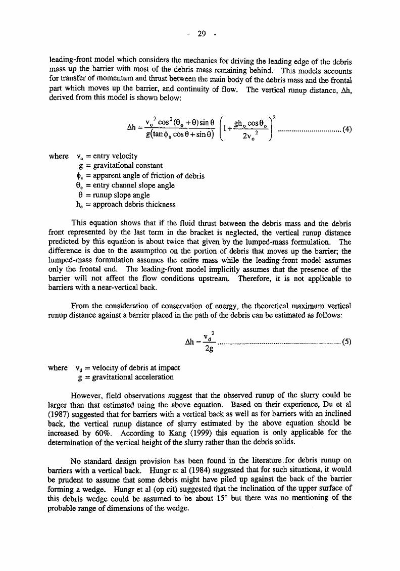
leading-front model which considers the mechanics for driving the leading edge of the debrismass up the barrier with most of the debris mass remaining behind. This models accountsfor transfer of momentum and thrust between the main body of the debris mass and the frontalpart which moves up the barrier, and continuity of flow. The vertical runup distance, Ah,derived from this model is shown below:

AH = ~ ^ : - 1 H--2-^ SL /4)g(tan(|>a cos 6 +sinO) [ 2v0

2 J

where v0 = entry velocityg = gravitational constant

<|)a = apparent angle of friction of debris60 = entry channel slope angle6 = runup slope angle

h0 = approach debris thickness

This equation shows that if the fluid thrust between the debris mass and the debrisfront represented by the last term in the bracket is neglected, the vertical runup distancepredicted by this equation is about twice that given by the lumped-mass formulation. Thedifference is due to the assumption on the portion of debris that moves up the barrier; thelumped-mass formulation assumes the entire mass while the leading-front model assumesonly the frontal end. The leading-front model implicitly assumes that the presence of thebarrier will not affect the flow conditions upstream. Therefore, it is not applicable tobarriers with a near-vertical back.

From the consideration of conservation of energy, the theoretical maximum verticalrunup distance against a barrier placed in the path of the debris can be estimated as follows:

where vd = velocity of debris at impactg = gravitational acceleration

However, field observations suggest that the observed runup of the slurry could belarger than that estimated using the above equation. Based on their experience, Du et al(1987) suggested that for barriers with a vertical back as well as for barriers with an inclinedback, the vertical runup distance of slurry estimated by the above equation should beincreased by 60%. According to Kang (1999) this equation is only applicable for thedetermination of the vertical height of the slurry rather than the debris solids.

No standard design provision has been found in the literature for debris runup onbarriers with a vertical back. Hungr et al (1984) suggested that for such situations, it wouldbe prudent to assume that some debris might have piled up against the back of the barrierforming a wedge. Hungr et al (op cit) suggested that the inclination of the upper surface ofthis debris wedge could be assumed to be about 15° but there was no mentioning of theprobable range of dimensions of the wedge.

- 30 -

4.5 Dynamic Interaction upon Debris Impact at Barrier

4.5.1 Pefcrjs Impact

(1) pmpirical Methods. The debris impact loading on a barrier is sometimesestimated assuming a hydrostatic pressure distribution together with an 'enhancement factor'.In Switzerland, the 'enhancement factor' is typically assumed to be 3, whereas in Austria, thisis usually taken to be 3 to 5 (Thurber Consultants Ltd, 1984),

The basis of such empirical approaches is not clearly documented but these may becompared to measurements reported in the literature. For example, Scotton & Deganutti(1997) used a 9.5 m-long flume together with coal slag with an average particle size of5.7 mm and different fluids to examine the effect of viscosity on the impact pressure onbarriers. The flume was inclined at 10°, 15° and 20° in the model tests. The results areexpressed in terms of the ratio of the measured impact pressure to the hydrostatic pressure atthe base. This ratio was found to fall within a wide range (between about 2.5 and 7.5), witha mean value of 5.3 for a more viscous flow and 3.5 for a less viscous fluid. The impactpressure in excess of the hydrostatic pressure is likely to be related to the velocity head of thedebris at impact but no information on debris velocity is given in the paper to allow anindependent data interpretation. Although the mean values are similar to the empiricalvalues adopted, it is noteworthy that the scatter of the measurements is considerable.

Wu et al (1993) reported that empirical impact pressures were prescribed for thedesign of barriers in Russia. The impact pressure is dependent on the magnitude of debrisflow events, the flow depth and the particle size of the entrained materials. An example ofsuch a prescriptive design approach is shown in Table 9.

(2) Analytical Methods. The average debris impact pressure imposed on a massbarrier can be estimated based on consideration of the rate of loss of momentum upon impact(Hungr et al, 1984; Du et al, 1987; Matsushita & Ikeya, 1992; PWRI, 1988), as follows:

p-pdvd2sinp (6)

where p = average impact pressurepd = density of debrisvd = velocity of debris at impactp = angle between the impact face of barrier and the debris motion direction

The average impact pressure is assumed to be uniform over the depth of the debris.

Field measurements of debris impact load may-be interpreted using the above equation.The results of a Japanese study on the field measurement of debris impact loads were reportedby Wu et al (1993). In the study, the impact load on a 15 cm by 15 cm plate was recorded(see Table 10). Figure 15 shows that the measured values are up to several times greaterthan the computed values using Eq. (6) assuming direct impact (i.e. p= 90°). Wu et al (1993)suggested that most of the measurements could have been influenced by boulders or hardinclusions hitting the sensors.

Another instrumented field study of debris impact pressure, velocity and density of

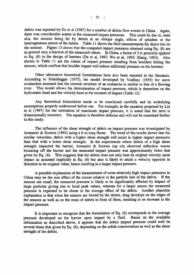
- 31 -

debris was reported by Du et al (1987) for a number of debris flow events in China. Again,there was considerable scatter in the measured impact pressures. This could be due to, interalia, the sensors being hit by debris at an oblique angle, effects of splashes or theheterogeneous nature of the debris. Table 11 shows the field measurements for direct hits onthe sensors. Figure 15 shows that the computed impact pressures obtained using Eq. (6) arein general only a fraction of the measured values. In China, a factor of 3 is generally appliedto Eq. (6) in the design of barriers (Du et al, 1987; Wu et al, 1993; Zhang, 1993). Alsoshown in Table 11 are the values of impact pressure resulting from boulders hitting thesensors, which confirm that boulder impact will induce additional pressure on the barriers.

Other alternative theoretical formulations have also been reported in the literature.According to Scheidegger (1975), the model developed by Voellmy (1955) for snowavalanches assumed that the internal structure of an avalanche is similar to that of a flowingriver. This model allows the determination of impact pressure, which is dependent on thehydrostatic head and the velocity head at the moment of impact (Table 12).

Any theoretical formulation needs to be scrutinised carefully and its underlyingassumptions properly understood before use. For example, in the equation proposed by Linet al (1997) for the estimation of maximum impact pressure, it is noted that the term isdimensionally incorrect. The equation is therefore dubious and will not be examined furtherin this study.

The influence of the shear strength of debris on impact pressure was investigated byArmanini & Scotton (1992) using a 6 m-long flume. The trend of the results shows that forsimilar velocities, debris with a higher shear strength will result in higher impact pressuresthan that with a lower shear strength. In the experiments where debris of a high shearstrength impacted the barrier, Armanini & Scotton (op cit) observed reflection wavesbouncing off the barrier and the measured impact pressure was approximately twice thatgiven by Eq. (6). This suggests that the debris does not only lose its original velocity uponimpact as assumed implicitly in Eq. (6) but also is likely to attain a velocity opposite indirection to its original value, hence resulting in a larger impact pressure.

A possible explanation of the measurement of some relatively high impact pressures inChina may be the size effect of the sensor relative to the particle size of the debris. If thesensors are small, the measured pressure is likely to be significantly affected by impact oflarge particles giving rise to local peak values, whereas for a larger sensor the measuredpressure is expected to be closer to the average effect of the debris. Another plausibleexplanation is that when the sensors are buried by the debris, drag develops on the edges ofthe sensors as well as on the mass of debris in front of them, resulting in an increase in theimpact pressure.

It is important to recognise that the formulation of Eq. (6) corresponds to the averagepressure developed on the barrier upon impact by a fluid. Based on the availableinformation as described above, it appears that the debris impact pressure could well beseveral times that given by Eq. (6), depending on the solids concentration as well as the shearstrength of the debris.

- 32 -

4.5.2 Boulder Impact

Boulders can be entrained within landslide debris and it is important that suitableallowance be made in barrier design. According to Zhang et al (1996), the boulders willgenerally be in clusters aligning either traversely across the front or longitudinally along thedebris trail, with the largest boulder in the front, in a debris flow. They also reported thatboulders could stay afloat near the surge and travel at a velocity similar to that of the debris.The boulder size is, in general, dependent on the boulders that can be mobilised and thecapacity and content of the debris flow. An overview of selected methods in estimatingboulder impact load (Table 13) is given below.

PWRI (1988) recommended that the estimation of boulder impact force should bedetermined using the Hertz equation (Table 13), which was derived for an elastic sphereimpacting an elastic medium. In determining the boulder impact force, it was recommendedthat the velocity of the boulder should be taken as that of the debris flow and that the designboulder size should be taken as the maximum size which can be mobilised by the debris.Hungr et al (1984) suggested that the design boulder should be assumed to be a sphere withits diameter equal to the flow depth.

As the actual impact may not be perfectly elastic and that material crushing may occurat the contact, Hungr et al (1984) cautioned that the contact forces computed using the Hertzequation could be extremely conservative and suggested to reduce them nominally by a factorof 10.

Zhou et al (1991) reported field measurements in Japan which showed the measuredboulder impact forces to be about 4% to 11% of those computed using the Hertz equation.Based on the above measurements, they suggested that the boulder impact force computedusing the Hertz equation should be reduced by a factor of 5 to 10.

For certain structural elements (e.g. bridge piers), flexural deformations could be moreimportant than contact deformations in governing the magnitude of the forces generated byboulder impact. The impact forces on such structures can be estimated by equating thekinetic energy of the boulder with the work (or energy) expanded by the structure inundergoing flexural deflection, as follows:

where F = impact forcemb = boulder mass

P = angle between the impact face of barrier and the debris motion directionvb .= boulder velocity

KB = stiffness factor of the barrier structure

The flexural stiffness factors for the case of simply-supported and cantilever structuresare derived and summarised in Table 13. It can be seen that the impact force is proportionalto the bending stiffness of the structure.

According to Huang (1996), a slightly different form of the above equation wasadopted by the Chengdu Railroad Research Institute in the estimation of boulder impact force

33 -

(see Table 13 - Compressible barrier method). The coefficient i] denotes the proportion ofkinetic energy of the boulder imparted onto the barrier. According to Huang (op cit), thevalue of TI may be assumed to be 0.3 for a circular impact surface, and that the sum of thecoefficients of elastic deformation of the boulder and barrier may be assumed to be0.005 m/kN, which was for bamboo or wooden rafts impacting bridge piers. A similarequation with similar coefficients has been put forward by AASHTO for estimating shipcollision on bridge piers (Xanthakos, 1995). It is of interest to note that the formula adoptedby the Highways Department (1993) in estimating the impact force from a vehicle is derivedalong the same principle as above whereby the kinetic energy of the vehicle immediatelybefore impact is equated to the work expanded in squashing the vehicle (Table 13).

Wu et al (1993) reported that the boulder impact force could also be estimated fromthe change in momentum of the boulder upon impact, with the duration over which thechange in momentum takes place being assumed to be 1 second.

Zhang et al (1996) noted that when a boulder impacts a barrier, the impact load willpropagate at the velocity of the compressive wave generated, from the contact point to otherparts of the boulder. The formula for estimating the force using wave theory depends on,inter alia, the velocity of compression wave and the contact area. The former is generallydetermined either from the elastic modulus and the density of the boulder, or is taken to beabout 4000m/s. The latter, however, is very difficult to estimate with confidence inpractice.

Haller & Gerber (1998) conducted a series of field tests in which boulders up to2 700 kg in weight impacted flexible rock fences at velocities of up to 27 m/s. They used ahigh-speed (54 frames/second) camera to capture the trajectory and the deceleration processof the boulder. They noted that after the first contact with the rock fence, the boulderunderwent a displacement of up to 5 m before coming to a halt. The entire process ofbringing the boulder to rest lasted about 0.3 second and the peak deceleration force wasestimated to range from 200 kN to 600 kN. For stiffer systems, the impact duration will bemuch shorter and consequently very large impact forces will result.

The process of boulder impacting onto a barrier may also be studied using computermodelling. An example is LS-DYNA, a non-linear 3-D finite element program which hasbeen used recently to simulate a boulder impacting a steel fence (Ove Arup & Partners HongKong, 1998) to determine its probable deformations and stresses.

5. SUMMARY AND DISCUSSION

5.1 Debris Mobility

The back-analysis of the mobility of the natural terrain landslides by Hungr (1998),Ayotte & Hungr (1998) and Chen & Lee (1998) has demonstrated that the continuum modelcould reasonably predict the downslope motion of landslide debris. The favourablecomparison between the observed and back-calculated debris velocity for the Tsing Shandebris flow using DAN as outlined in Section 4.4.2 is also an indication of the reliability ofthese continuum models. These back-analyses suggest that the friction model can be areasonable rheological model for simulating the average shear resistance at the base of bothopen hillside failures and channelised debris flows.

- 34 -

In the friction model the apparent angle of friction (<j>a) of the landslide debris is acritical parameter that controls the mobility of the debris. It is a function of the mechanismof debris movement, structure of the debris and its behaviour under shear. The dynamicpore water pressures generated during the downslope journey of the debris have beeninvestigated by researchers by means of laboratory shear tests and flume tests (e.g. Sassa,19&8; Iverson & Lehusen, 1989; Reid et al, 1997). Sassa (1988) advocates the use of high-speed ring shear apparatus on the finer fraction of the debris to assess <j>a.

The behaviour of the debris as well as its composition are likely to vary within thedebris mass and along its path, i.e. there is temporal and spatial variations in the rheology ofthe debris mass along the debris trail In view of this, Hungr et al (1997) opined that "it isunlikely that satisfactory predictions of the dynamic behaviour (of debris) can be achievedbased on laboratory-derived constitutive relationships. Empirical determination of the bulkrheology, based on back-analysis of actual events, is more realistic." Figure 16 shows thatthe apparent angles of friction obtained from back-analyses of some natural terrain landslidesare comparable to the corresponding travel angles observed in the field. Hence, a possiblemeans to estimate the apparent angle of friction of the debris for a landslide of a given volumeis to base it on the travel angle of landslides of similar volume and mechanism.

Figure 17 shows a compilation of travel angles for some natural terrain landslides inHong Kong. It can be seen that the debris mobility is a function of the debris volume andthe mechanism of debris motion. For a given landslide volume, the travel angle of the debrisfrom a channelised debris flow is generally smaller than that from an open hillside failure (i.e.a channelised debris flow is more mobile than an open hillside failure). The debris mobilityof the latter increases with the scale of failure whereas that for the former appears to beindependent of it. These data imply that a small channelised debris flow is as mobile as alarge one. For open hillside failures, the travel angle of the debris is generally between 25°and 40° for debris volumes less than 400 m3, and ranges from 20° to 25° for volumes equal toor exceeding 400 m3. The travel angle for channelised debris flows typically ranges between20° and 25°. Based on these available data and the correlation shown in Figure 16, theapparent angle of friction could conservatively be taken as 20° for channelised debris flows.For open hillside failures, the apparent angle of friction could be taken as 25° for volumes lessthan 400 m3 and 20° for volumes equal to or exceeding 400 m3. Given a certain landslidevolume, there could be a wide range of debris mobility (in terms of mobility angle).Therefore, the lower bound values of travel angle in Figure 17 are suggested to be taken as theapparent angle of friction for design purposes, to ensure that the mobility of the debris wouldnot be underestimated.

Hungr (1998) and Ayotte & Hungr (1998) have found that, in general, the Voellmymodel tends to better predict the distribution of debris than the friction model for channeliseddebris flows. The latter commonly predicts slightly higher debris velocity than the former.Therefore, the Voellmy model, together with an apparent friction angle, <|>a = 11° and aturbulence coefficient, £ = 500 m/s2 (which have been found to be appropriate by Hungr(1998) and Ayotte & Hungr (1998)), is suggested to be used to assess the mobility of debrisflows.

Unlike the back-analysis of a landslide where the width of debris along its path isknown, the prediction of debris mobility using a two-dimensional model, such as DAN,requires the knowledge of debris width in advance. The compilation of the width profile

- 35 -

along the debris path should be made with due reference to that observed in past landslides atthe site and the local topographical conditions.

As there are very few measured data available regarding the velocity of debris, theresults of DAN analysis of some twenty natural terrain landslides in Hong Kong have beenfurther examined in an attempt to develop appropriate empirical correlations to facilitate theassessment of debris mobility. Although these are computed values, their quality may not beconsiderably inferior to the field measurements because the continuum models such as DAN(Hungr, 1995) and the one developed by Chen & Lee (1998)) satisfy the principles ofconservation of mass, energy and momentum. They have also been calibrated against fieldobservations.

The maximum debris frontal velocity for each natural terrain failure back-analysed byHungr (1998) and Ayotte & Hungr (1998) using DAN is plotted against the correspondingmaximum debris thickness in Figure 18. There is considerable scatter in the DAN data.Also shown in this figure are predictions from various flow models discussed in Section 4.4.2.There appears to be no well defined correlation between the computed maximum debrisfrontal velocity, maximum debris thickness and the average slope gradient for open hillsidefailures and none of the flow models seems to be able to adequately describe these computeddata. The values of the maximum debris velocity and the maximum debris thickness havebeen carefully selected along the debris trail to avoid possible errors resulting from numericalinaccuracies in the model near the source area. Nonetheless, the data point marked with anasterisk in Figure 18 was believed to have been influenced by the initial conditions as thefrontal velocity was abruptly reduced by half after reaching the maximum.

In this study, the debris velocity has been back-calculated from the super-elevationdata reported by King (1996) at two locations for the 1990 Tsing Shan debris flow. Thesevelocity data are shown in Figure 18 for comparison. For channelised debris flows, it seemsthat the estimates made by the empirical model by Du et al (1987) are quite similar tocomputed values using DAN as well as the back-calculated velocity data from super-elevationmeasurement for Tsing Shan debris flow. However, owing to the limited data currentlyavailable, it may be premature to draw conclusion as to which flow model and the associatedparameters will best describe the motion characteristics of debris flows.

Figure 19 shows the maximum debris frontal velocity and maximum debris thicknessobtained from DAN and plotted against the corresponding landslide volume. The observedmaximum debris thicknesses along the debris trails reported by Wong et al (1998) for naturalterrain landslide studies on Lantau Island are also shown in Figure 19b. Despite the scatter,both the maximum debris frontal velocity and maximum debris thickness tend to increasewith debris volume. A pragmatic approach is proposed by grouping the data into fourvolume ranges as shown in Figure 19 and selecting the upper bound values of the debrisvelocity and debris thickness within each volume range for design. The proposeddemarcation, although arbitrary, takes due consideration of clustering of the data. Thechoice of upper bound values is to account for the scatter in data and to ensure that aconservative estimate of the debris impact pressure is obtained in the absence of a detailedassessment of debris mobility.

This empirical approach makes no distinction between open hillside failures andchannelised debris flows, i.e. for a given landslide volume, the debris velocity and debris

36 -

thickness will be the same for channelised debris flows and open hillside failures. This isbecause the currently available data are very limited and as shown in Figure 19 there is nodistinct trend that debris velocity and debris thickness are dependent on mechanism ofmovement. However, the proposed approach should be reviewed when additionalinformation on debris mobility becomes available.

" Although the upper bound values for each volume range have been proposed fordesign, these values may not be adequate under some circumstances because the existing dataset is very limited, e.g. there are very few data for failures with volume exceeding 3 000 m3.Therefore, it is prudent to compare these values with data from other sources, as far aspossible, such as velocity estimated from super-elevation data or back-analysis of site-specificdata/failures.

5.2 Runout and Runup Distance

The debris velocity values determined using the above empirical approach are fordebris travelling on the slopes. Suitable adjustment to this velocity is necessary when thereis an abrupt change in gradient along the debris trail, e.g. where the slope flattens out. Theformulations for the determination of runout and runup given in Tables 7 and 8 may be used.These can.be broadly grouped into two categories: lumped-mass (sled) model and leading-edge model.

Chu et al (1995) carried out some runup measurements of dry gravel flowing down a5 m long flume onto the back side of a barrier placed at the tail-end of the flume. Therunning surface of the flume and the barrier was lined with sheet metal to keep the frictionalresistance small in order to achieve a wide range of approach velocity. The inclination ofthe flume and the back of the barrier was varied. Their measurements allow an evaluation ofthe three models in Table 8. Figure 20 shows the measurements and predictions by the threemodels. There is considerable scatter in the data. The sled model with no correction forslope gradient overestimates the runup distance by a factor of about 4. The sled model withmomentum correction and the leading-edge model tend to predict runup distances closer tothe field measurements with the former tending to slightly underestimate the runup distancewhile the latter slightly overestimates it. A closer examination of the data suggests thatTakahashi's model gives fairly reasonable estimate for runup slope angle in the range of 20°and 40° which is similar to the inclination of the slope surface of an earth embankment.

Based on this comparison and the consideration that the leading edge model seems togive runouts that compare quite favourably with field observations, it is suggested that theleading-edge solution be used for the prediction of debris runup on the back of a barrier aswell as the runout distance and debris velocity on the runout path.

5.3 Debris

In assessing the various approaches put forward by different investigators for thedetermination of impact loading, more weight has been given to those which are supported byfield measurements or calibrated against field observations.

- 37 -

Among the various formulations available for the estimate of debris impact pressure,the one derived from rate of fluid losing its momentum upon impact onto a rigid surfaceclosely resembles the dynamics of debris impacting onto barriers. This equation is based onthe assumption that the impacting fluid has no shear strength. Unlike fluid, landslide debrisexhibits shear strength which varies broadly according to its water content. The exactrelationship between the shear strength of the debris and debris impact pressure is not wellunderstood. However, the work by Armanini & Scotton (1992) and Scotton & Deganutti(1997) showed that the debris impact pressure is dependent on the shear strength of the debrisand their measurements indicated that it could be up to twice that given by Eq. (6). Thecomprehensive field measurements of debris impact pressure carried out in China showed thatthe measured debris impact pressure could be 2 to 4 times that given by Eq. (6). As a firstapproximation, the debris impact pressure could be taken to be at least three times that givenby Eq. (6), i.e.

P = 3pdvd2sinp (8)

5.4

Wu et al (1993) and Zhang et al (1996) reported a number of landslide events in Chinawhere structures were damaged by boulders. They gave information on the flowcharacteristics of the debris and estimated the loads under which these structures would havefailed. It seems that the failure capacities reported by the original authors might not haveaccounted for the dynamic effects and hence they would likely be lower than actual valuesobserved in the field. This information has allowed a comparison of the boulder impactloads calculated using the different formulae given in Table 13. In some cases, theinformation needed for the computation is not readily available from the published papers andfor the purposes of the present comparative study, typical values have been adopted. Theresults are summarised in Table 14.

It can be seen that there is a wide scatter in the predicted results. The impact forcesestimated using the Hertz equation are about one to two orders of magnitude higher than theestimated ultimate capacity of the damaged structure. It seems that the impact forcescomputed using the Hertz equation are unduly conservative and can be reduced by a factor ofat least 10. On the other hand, the formula adopted by the Chengdu Railroad ResearchInstitute consistently predicts much lower impact forces which are only a small fraction of theultimate capacity of the barriers. The principal reason for the underestimation of the impactforce is likely to be due to the inappropriate use of the coefficient of elastic deformationderived from bamboo and wooden rafts which are much more flexible and ductile thanboulders.

The momentum equation given in Table 13 also tends to underestimate the impactforces which suggests that the assumed impact duration of 1 second may not be appropriate.This also highlights the sensitivity of the estimates to the assumption of impact durationwhich is very difficult to determine reliably.

The flexural stiffness equation and the wave theory tend to give estimates closer to thecomputed ultimate capacities of the structures. It should be noted that in the reported casestudies, the only established information is that the boulder impact force exceeded the failure

- 38 -

capacity of the structure and therefore no definite conclusion can be drawn as to the relativereliability of the two formulae. It is noteworthy, however, that the wave theory requires theknowledge of the contact area at impact, which is very difficult to determine. The stiffnessfactors given in Table 13 for use in the flexural stiffness equation are for columnar structuresor beam structures which are different from those for mass wall structures. In summary, theorder of magnitude of the boulder impact load could be estimated using the flexural stiffnessmethod, or taken to be nominally one-tenth of that given by the Hertz equation. Asdiscussed in Section 4.5.2 the boulder impact could also be assessed by means of computerprograms that have been calibrated against measurements.

The above exercise serves to illustrate the uncertainties in the predictions. In practice,expedients such as the possible incorporation of a soft cushion of suitable material, e.g. rubbertires, in front of the barrier may assist in reducing boulder impact loads by extending theduration of impact (see Plate 15).

6. SUGGESTIONS FOR DESIGN OF BARRIERS

6.1 General

A review of the design methodology for debris-resisting barriers has been carried outand is summarised in Section 4. These approaches have been compared and evaluated in thelight of field measurements as far as possible (Section 5). Suggestions for the design ofdebris-resisting barriers have been drawn up based on this review to facilitate design.

Design of barriers begins with the identification and characterisation of the naturalterrain hazards at a site. Different approaches can be used to determine the design event, asoutlined in Section 4.3. The approach should be selected with due consideration of theavailable data on previous landslide activity, local topographical and geological conditions,and the limitation of the approach itself. The pros and cons of different methods arediscussed in Section 4.3. After estimating the scale of the design event and its probablelocation, the assessment of the landslide debris mobility and debris impact loads can becarried out.

Two approaches may be used for estimating debris mobility:

(a) analytical approach, and

(b) empirical approach.

These are presented in Section 6.2 below. The suggested procedures for assessmentof debris impact loads are presented in Sections 6.3 and 6.4.

6.2 Debris Mobility

6.2.1 Analytical Approach

Continuum models can be used to estimate debris mobility. However, due to lack ofrelevant experience, only those models, such as DAN, a two-dimensional model by Hungr

- 39 -

(1995) and the three-dimensional model developed by Chen & Lee (1998), which have beencalibrated against field measurements, should be used. A frictional rheological model(Table 6) can be used for both open hillside failures and channelised debris flows. Theapparent angle of friction can be determined by means of high-speed ring shear as suggestedby Sassa (1988) or can be taken as the travel angle of landslide debris observed in failures ofsimilar scale and mechanism. It is suggested that the apparent angle of friction can be takenas 25° and 20° for open hillside failures with debris volumes below and equal to or above400 m3 respectively. For channelised debris flows, the friction model with an apparent angleof friction of 20° or the Voellmy model with an apparent angle of friction of 11° and aturbulence coefficient of 500 m/s2 can be used.

If a two-dimensional continuum model, such as DAN, is used, the debris width profilealong the debris trail is required as input. This should be compiled with due reference to thatobserved in past landslides at the site and the local topographical conditions.

6.2.2 Empirical Approach

The maximum debris velocity and maximum debris thickness on the slope can bedetermined based on the estimated debris volume as shown in Figure 21. The values ofdebris velocity and debris thickness given in Figure 21 apply to both open hillside failures andchannelised debris flows. The assessment of debris runout can be carried out using theleading-edge model (Table 7). The apparent angle of friction is suggested to be taken as 25°and 20° for open hillside failures with volumes less than and equal to or exceeding 400 m3

respectively. For channelised debris flows, a friction model with an apparent angle offriction of 20° is suggested. For barriers with a sloping back, the debris runup can beestimated using the leading edge model given in Table 8.

It is prudent to temper the debris mobility data derived from these approaches withinformation from other sources, such as velocity estimated from super-elevation data, as far aspossible.

6.3 Debris Impact

The landslide debris impact pressure can be estimated from the following equation:

P=:3pdvd2sinp ............(8)

where p = average impact pressurepd = density of debrisvd =? velocity of debris at impactp = angle between the impact face of barrier and the debris motion direction

The average impact pressure can be assumed to be uniform over the depth of thedebris.

- 40

6.4 Boulder Impact

The impact loading due to boulders in the landslide debris can be estimated using theformulation which accounts for the flexural stiffness of the barrier or it can be taken as one-tenth of that predicted by the Hertz equation (Table 13). The boulder can be assumed totravel at the same velocity as the debris mass. The size of the boulder that could beentrained depends on the size of boulder in the area as well as the thickness of the debrismass.

6.5 Stability Check and Structural Design

Barriers, like retaining walls, can fail by sliding, overturning, or as a result of bearingcapacity failure. Structural failures of the barrier are also possible- The stability of thebarrier against different modes of failure should be checked in accordance with Geoguide 1(GEO, 1993). Due to their transient nature, the partial load factor for the debris and boulderimpact loads may be taken as unity. The structural design of the barrier should be carriedout in accordance with the requirements of the relevant structural code and standards.

As the debris may occur in pulses, the stability of the barrier should also be checkedfor various scenarios, including:

(a) first frontal impact by debris,

(b) subsequent impact with debris accumulated behind thebarrier, and

(c) static loading on the wall when the debris has come to restafter impact.

For scenarios involving a layer of debris riding on previously deposited debris, theeffect of the weight of the upper debris acting as surcharge on the underlying layers need tobe accounted for.

7, OTHER DRSTGN CONSTDHR ATTHNTS

The retention capacity of the barrier is affected by the size of the buffer zone, theheight of the barrier and the storage angle which is the angle between the upper surface of thedebris piled up behind the barrier and the horizon. The location of the barrier should bechosen judiciously to allow ample space to accommodate the volume of the design debrisevent. It is also necessary to ensure that the barrier is high enough to account for thepossibility of debris runup. PWRI (1988) recommended that the storage angle could betaken between horizontal and 1/2 to 2/3 of the channel bed angle. Possible bulking of thedebris material should be taken into account in assessing the required retention capacity.The amount of bulking will be dependent on the original structure of the material King(1996) reported that for Tsing Shan debris flow, the bulking factor was found to be about 8%.

There are many types of barriers, e.g. counterfort walls, gabion walls, reinforced fill

41

structures, and other types of gravity structures. The choice of barrier type should be madetaking due cognisance of the construction and maintenance costs, land take and buildability.Whether the barrier is to be designed as a sacrificial or permanent structure should also beconsidered. The barrier should be well maintained, e.g. by regular removal of debrisaccumulated behind the barrier, to ensure there is adequate storage capacity.

For a barrier that straddles a streamcourse, special provisions such as decanting orstraining structures that allow normal streamflow should be incorporated in the design.Figure 22 shows a variety of barrier design with different straining and drainage provisions.

An assessment of the likely path to be traversed by landslide debris should be madetaking due consideration of, inter alia, the topography and ground surface characteristics.Avulsion may occur when a debris mass blocks its own path, e.g. a stream channel, causing itto divert. This could lead to the spreading of debris material to other areas adjacent to theoriginal flow path. For example, mobile debris when passing through a bend may bedeflected away from its original path. Davies & Hall (1992) reported an incident in NewZealand where the super-elevation effect of the debris in a bend caused it to overflow thechannel banks and shot into the adjacent facilities killing four people.

In the event where the debris impact loading is considerable, a second line of defenceinvolving some form of sacrificial elements, e.g. rows of wooden piles, rubber tires, or rubbleplaced behind the barrier can 'soften' the impact on the primary barrier and minimise itsdamage.

Due consideration should also be given to selecting an appropriate constituent materialfor a barrier. For example, combustible material should be avoided where the risk of hill fireis high. There has been an incident in Hong Kong in 1989 in which the geosynthetic gabionmaterial of four gabion barrier walls was badly damaged (Au & Chan, 1991).

8. RECOMMENDED R&D STUDIES

A number of areas requiring development work have been identified. In general,there is a lack of consistent terminology used in the different case histories for describing thevarious landslide phenomena, such as debris flow and debris flood. Therefore, a standard setof terminology should be developed to facilitate better communication and possibleextrapolation of empirical data.

The debris mobility and the interaction between debris and barrier are keyconsiderations in the design of debris-resisting barriers. Further studies by means ofliterature review and laboratory and field studies should be conducted to improve the currentstate of knowledge on the mechanisms of natural terrain landslides and the relevant factorscontributing to failure and mobility of debris, with a view to developing a practical schemefor the classification of mechanisms of debris movements, assessment of debris mobility andidentification of mobile mechanisms.

Investigation into the impact loading on barriers may be further examined throughlaboratory simulation testing and field trials. For example, flume tests and centrifuge studiescould provide valuable insights into the effects of various factors, such as shearing resistance

- 42

of debris, water content of debris, etc, on the impact load. These measurements can alsoprovide a basis for critical examination of the various existing formulations as well as thesuggested methods, for possible improvement in methodology to estimate impact load.

Some exploratory work has been carried out with the use of advanced numericalmodels (e.g. FLAG, LS-DYNA) to assist in gaining an insight into the impact process.Suitable formulation needs to be used to overcome the difficulty in modelling the large strainbehaviour of a particulate medium associated with debris motion. Numerical models basedon a particulate formulation may be worthy of trial use to assess the behaviour of debrisimpact on a barrier.

9. CONCLUSIONS

Barriers are, in some situations, a practical mitigation measure that can help to reducethe risks posed by natural terrain landslide hazards to vulnerable facilities. The rationaldesign of barriers, in particular the assessment of the design landslide events and the likelyimpact loads, is however fraught with difficulties. Although some of the design procedurescan be based on theoretically rigorous methods, the determination of many of the designparameters is not an exact science and often involves field estimates, rules of thumb andengineering judgement. An under-designed barrier can result in disastrous consequencesand it can provide a false sense of security.

The reliability of the barrier design depends critically on the quality of information forassessing the locations of potential failure or debris detachment and on the likely volume,mobility, travel path and deposition of landslide debris. The importance of collecting goodquality data locally such as volume, velocity (e.g. to be deduced from super-elevation data)and thickness of landslide debris cannot be over-emphasised.

Various approaches put forward for evaluating the impact loads on barriers have beenreviewed and these illustrate, inter alia, the considerable scatter in the predictions as well as insome of the reported field measurements. Based on the present state of knowledge, somesuggestions (summarised in Figure 21) are put forward to facilitate the assessment of debrismobility and debris impact loads in the design of landslide debris-resisting barriers. Giventhe developments in the subject, the suggestions are intended to be interim. They will bereviewed and updated when new data and results of further research become available.

Further research is needed to gain a better fundamental understanding of the nature andmechanisms of natural hillside failures in Hong Kong and to improve the methods forassessment of debris mobility and debris impact loads under local conditions.

Pending the results of further R&D work, it is strongly recommended that theassessment of debris impact loads on barriers should be conducted in a cautious andconservative manner, with due allowance made for the uncertainties involved.

43

10 REFERENCES

Armanini, A. & Scotton, P. (1992). Experimental analysis on the dynamic impact of adebris flow on structures. Proceedings of the International SymposiumTNTERPRAEVENT 1992: Bern, pp 107-116.

Au, S.W.C. & Chan, C.F. (1991). Boulder Treatment in Hong Kong. Selected Topics inGeotechnical Engineering - Lumh Volnt^ edited by K.S. Li, pp 39-71.

Ayotte, D. & Hungr, O. (1998). Runout Analysis on Debris Flows and Debris Avalanchesin Hong Kong* Report prepared for the Geotechnical Engineering Office, HongKong,90p.

Chan, Y.C., Chan, C.F. & Au, S.W.C. (1986). Design of a boulder fence in Hong Kong.Proceedings of the International Conference on Rock Engineering and Excavation inftp Urban Environment, Hong Kong, pp 87-96.

Chau, K.T., Chan, L.C.P., Wu, J.J., Liu, J., Wong, R.H.C. & Lee, C.F. (1998). Experimentalstudies on rockfall and debris flow. Proceedings of the One Day Seminar onPlanning. Design and Implementation of Debris Flow and Rockfall Hazards MitigationMethods. Hong Kong, pp 115-128.

Chen, C.L. (1986). Bingham plastic or Bagnold's dilatant fluid as a rheological model ofdebris flow? Proceedings of the Third International Symposium on RiverSedimentation, Mississippi, pp 1 624-1 637.

Chen, H. & Lee, C.F. (1998). Debris flow modelling with three-dimensional. Lagrangianfinite elements. Proceedings of the One Day Seminar on Planning. Design andImplementation of Debris Flow and Rockfall Hazards Mitigation Methods. HongKong, pp 29-45.

Chu, T., Hill, G., MeClung, D.M., Ngun, R. & Sherkat, R. (1995). Experiments on granularflows to predict avalanche runup. Canadian Geotechnical Journal, vol. 32,pp 285-295.

Corominas, J. (1996). The angle of reach as a mobility index for small and large landslides.Canadian Geotechnical Journal, vol. 33, pp 260-271.

Cruden, DJM & Varnes, DJ. (1996). Landslide types and processes. Landslides;Investigation and Mitigation, edited by A.K. Turner & R.L. Schuster, TransportationResearch Board Special Report 247, National Research Council, pp 36-75.

Czerny, R (1998). Wildhachsperren aus Beton und Stahlbeton. Medieninhaber undHerausgeber: Zement +• Beton Handels- und Werbeges.m.b.H im Auftrag derosterreichischen Zementindustri, 18 p.

Davies, T.R. (1993). Research needs for debris flow disaster prevention. Proceedings ofHydraulic Engineering993. San Francisco, pp 1 284-1 289.

44 -

Davies, T.R. & Hall, RJ. (1992). A realistic strategy for disaster prevention. Proceedingsof the International Symposium TNTFrRPgAKVHNT 1992. Bern, pp 381-390.

Dawson, D.F., Morgenstern, N.R. & Gu, W.H. (1992). Instability Mechanisms InitiatingFlow Failures in Mountainous Mine Waste Dumps. University of Alberta, 80 p.

De&atale, J.S., Fiegel, G.L. & Fisher, G.D. (1996). Response of the Geobrugg Cable NetSystem to Debris Flow Loading. California Polytechnic State University, 90 p.

Du, R., Kang, Z., Chen, X. & Zhu, P. (1987). A Comprehensive Investigation and ControlPlanning for Debris Flow in the Xiaojiang River Basin of Yunnan Province. SciencePress, 287 p (in Chinese).

Duffy, J.D. (1998). Case studies on debris and mudslide barrier systems in California.Proceedings of the One Day Seminar on Planning. Design and Implementation ofDebris Flow and Rockfall Hazards Mitigation Methods. Hong Kong, pp 77-90.

Evans, N.C., Huang, S.W. & King, J.P. (1997). The Natural Terrain Landslide Study -Phases I and TI (Special Project Report, SPR 5/97). Geotechnical Engineering Office,Hong Kong, 119 p.

Evans, N.C. & King, J. (1998). The Natural Terrain Landslide Study: Debris AvalaqcfceSusceptibility (Technical Note TN 1/98). Geotechnical Engineering Office, HongKong, 96 p.

Fang, Y.S. & Zhang, Z.Y. (1988). Kinematic mechanism of catastrophic landslides andprediction of their velocities and travelling distance. Proceedings, of thff FifthInternational Symposium on Landslides^ Toronto, vol. 1, pp 125-128.

Franks, CAM. (1998). Study of Rainfall Induced Landslides on Natural Slopgs in theVicinity of Tung Chung New Town. Lantau Island (GEO Report No. 57).Geotechnical Engineering Office, Hong Kong, 102p.

Franks, CA.M. & Woods, N.W. (1997). Natural Terrain Landslide Study: PreliminaryReview of-natural Terrain Landslide Hazard Mitigation Measures (Technical NpteNo. 8/97). Geotechnical Engineering Office, Hong Kong, 52p.

Frenette, R., Eyheramendy, D. & Zimmermann, T. (1997). Numerical modeling of dam-break type problems for Navier-Stokes and granular flows. Proceedings, pf tfog pi^tInternational Conference on Debris-Flow Hazards Mitigation: Mechanics, Predictionand Assessment. San Francisco, pp 586-595.

GEO (1993). Guide to Retaining Wall Design (ftengmde I V (Second Edition).'Geotechnical Engineering Office, Hong Kong, 267p.

Haller, B. (1999). Personal Communication

- 45 -

Haller, B. & Gerber, W. (1998). Field testing and design of high energy absorption rockfallbarriers. Proceedings Of the One Dav Seminar on Planning. Design andImplementation of Debris Flow and Rockfall Hazard. Mitigation Methods. HongKong, pp 99-104.

Highways Department (1993). Structures Design Manual for Highways and Railways.Hong Kong Government, 210 p.

Ho, K.K.S. & Wong, H.N. (1999). Lessons Learnt from Landslide Investigations.Presented at the Hong Kong Institution of Engineers Geotechnical Division TechnicalMeeting in July 1999, Hong Kong. (Unpublished).

Huang, Z. (1996). Engineering Techniques for Debris Flow Mitigation. China RailroadPress, 301 p (in Chinese).

Hungr, O. (1995). A model for the runout analysis of rapid flow slides, debris flows, andavalanches. Canadian Geotechnical Journal, vol. 32, pp 610-623.

Hungr, O. (1998). Mobility of Landslide Debris in Hong Kong: Pilot Back Analyses using aNumerical Model. Report prepared for the Geotechnical Engineering Office, HongKong, 50 p.

Hungr, O., Dawson, R., Kent, A., Campbell, D. & Morgenstern, N.R. (1997). Rapid flowslides of coal mines in British Columbia, Canada. Proceedings of Reviews inEngineering GeologyT Geological Society of America fin press).

Hungr, O. & Evans, S.G. (1996). Rock avalanche runout prediction using a dynamic model.Proceedings of the Seventh International Symposium on Landslides. Trondheim, vol. 1,pp 233-238.

Hungr, O. & McClung, D.M. (1987). An equation for calculating snow avalanche runupagainst barrier. Proceedings of the Davos Symposium on Avalanche Formation,Movement and Effects, pp 605-612.

Hungr, O., Morgan, G.C & Kellerhals, R. (1984). Quantitative analysis of debris torrenthazards for design of remedial measures. Canadian Geotechnical Journal, vol. 21,pp 663-677.

Hungr, O,, Morgan, G.C., VanDine, D.F. & Lister, D.R. (1987). Debris flow defences inBritish Columbia. Reviews in Engineering Geology. Volume VH PP 201-222.

Hungr, O., Sun, H.W. & Ho, K.K.S. (1999), Mobility of selected landslides in Hong Kong -pilot back-analysis using a numerical model. Proceedings of the Hong KongInstitution of Engineers Geotechnical Pivision Annual Seminar on Geotechnical RiskManagement. Hong Kong, pp 167-175.

Innes, J.L. (1983). Lichenometric dating of debris flow deposits in the Scottish Highlands.Earth Surface Processes and Landforms. vol. 8, pp 579-588.

46

Itasca Consulting Group (1995). FT AC-Fast L,agrangian Analysis of Continua. Version 3.3.Volume 1: User's manual.

Iverson, R.M. & Lehusen, R.G. (1989). Dynamic pore-pressure fluctuations in rapidlyshearing granular materials. Science, vol. 246, pp 796-799.

Japan Forest Conservation and Flood Control Association (1985). Forest Conservation inJapan. 66 p.

Julien, P.Y. & O'Brien, J.S. (1997). On the importance of mud and debris flow rheology instructural design. Proceedings nf the First International Conference on Debris-FlowHazards Mitigation: Mechanics. Prediction and Assessment. San Francisco,pp 350-359.

Kang, Z. (1996). Debris Flow Hazards and Their Control in China. Science Press, 118 p.

Kang, Z. (1999). Personal Communication.

Kang, Z., Wang S., Lee, C.F. & Law, K.T. (1999). A Study of Debris Flow HazardPrevention. The Jockey Club Research and Information Centre for LandslipPrevention and Land Development, Hong Kong, 33 p (in Chinese).

Kawaken (1998). Product Catalogue (in Japanese).

King, J.P. (1996). The Tsing Shan Debris Flow ^Special Project Report SPR 6/96).Geotechnical Engineering Office, Hong Kong, 3 volumes.

Koch, T. (1998). Testing various constitutive equations for debris flow modelling.Proceedings of the HeadWater 98 Conference (IAHS Publication No. 248)T Italy,pp 249-257.

Lau, K.C. & Woods, N.W. (1997). Review of Methods for Predicting the Travel Distance ofDebris from Landslides on Natural Terrain (Technical Note TN7/97). GeotechnicalEngineering Office, Hong Kong, 48 p.

Lin, P.S., Chang, WJ. & Liu, K.S. (1997). Retaining function of open-type Sabo dams.Proceedinp-s of the First International Conference on Debris-Flow Hazards Mitigation:Mechanics. Prediction and Assessment, San Francisco, pp 636-645.

Mak, N. & Bloomfield, D. (1986). Rock trap design for presplit rock slopes. Proceedingsof the International Conference tm Rock Engineering and Excavation in an UrbanEiodnmmeni, Hong Kong, pp 263-269.

Matsushita, T. & Dceya, H. (1992). Methods for the evaluation of debris flow countermeasures. Proceeding of the International Symposium TNTF.RPRAEVENT 1992.Bern, pp 337-348.

McClung, D.M. & Schaerer, P.A. (1985). Characteristics of flowing snow and avalancheimpact pressures. Annals of G1aHn^gy vol. 6, pp 9-14.

47

Mizuyama, T., Kobashi, S. & Ou, G. (1992). Prediction of debris flow peak discharge.Proceedings of the International Symposium INTER PR AE VENT IQQI Bernpp 99-108.

Morgan, G.C., Rawlings, G.E. & Sobkowicz, J.C. (1992). Evaluating total risk tocommunities from large debris flows. Proceedings of the Symposium onGeotechnique and Natural Ha/.arfe Vancouver, B.C. pp 225-236.

Morgenstern, N.R. (1978). Mobile soil and rock flows. Geotechnical Engineering vol 9pp 123-141.

Okubo, S., Ikeya, H., Ishikawa, Y. & Yamada, T, (1996). Development of new methods forcountermeasures against debris flows. Recent Developments on Debris Flows.Lecture Notes in Earth Science, vol. 64, pp 166-185.

Ove Arup & Partners Hong Kong (1998). Rockfall Fence - Assessment of ImpactResistance. Report prepared for the Housing Department, Hong Kong, 59 p.

Perla, R., Cheng, T.T. & McClung, D.M. (1980). A two-parameter model of snow-avalanche motion. Journal of Glaciology, vol. 26(94), pp 197-207.

Pierson, T,C, & Costa, I.E. (1987). A rheological classification of subaerial sediment-waterflows. Reviews JO .....Engineering Oeologyf Volume VnT pp 1-12.

Public Works Research Institute (1988). Technical Standard for the Measures AgainstDebris Flow (Draft). (Technical Memorandum of PWRI No. 2632). Japan, 45 p.

Reid, M.E., Lahusen, R.G. & Iverson, I. (1997). Debris-flow initiation experiments usingdiverse hydrologic triggers. Proceedings of the First International Conference onDebris-FlQW Hazards Mitigation: Mechanics,. Prediction and Assessment. SanFrancisco, pp 1-11.

Rickenmann, D, & Koch, T. (1997). Comparison of debris flow modelling approaches.Proceedings of the First International Conference on Debris-Flow Hazards Mitigation;

Jcsr Prediction and Assessment. San Francisco, pp 576-585.

Roberds, WJ. & Ho, K.K.S. (1997). A quantitative risk assessment and risk managementmethodology for natural terrain in Hong Kong. Proceedings of the First InternationalConference on Debris-Flow Hazards Mitigation: Mechanics, Prediction andAssessment, San Francisco, pp 207-218.

Sassa, K. (1988). Geotechnical model for the motion of landslide. Proceedings of the FifthInternational Symposium op Landslides. Lausanne, vol. 1, pp 37-55.

Sawada, T., Suwa, H. & Takahashi, T. (1999). Rainfall condition for the occurrence ofdebris flow in the Jiangjia Gully. China-Japan Joint Research on the Mechanism andthe Countermeasures for the Viscous Debris Flow, PP 11-17.

Scheidegger, A.E. (1975), Physical Asp^rts of Natural Catastrophes. Elsevier, 289 p.

- 48 -

Scotton, P. & Deganutti, A.M. (1997). Phreatic line and dynamic impact in laboratorydebris flow experiments. Proceedings "f the First International Conference onDebris-Flow Hazards Mitigation: Monies, Prediction and Assessment. SanFrancisco, pp 777-786.

Sun, H.W. (1998). Review of Fill Slope Failures in Hong Konp ("Special Project Report4/981. Geotechnical Engineering Office, Hong Kong, 86 p.

Takahashi, T. (1991). Debris Flow. IAHR Monograph, Balkema, 165 p.

Takahashi, T. & Yoshida, H. (1979). Study on the Deposition of Debris Flows. Part T -Deposition due to Abrupt Change nf Bed Slope. Annuals, Disaster PreventionResearch Institute, Kyoto University, vol. 22, paper B-2.

Thommen, R.A. (1998). Testing and experiences gained in the field with flexible wire ropenetting barriers to retain mud and debris flow. Proceedings of the One Day Seminarnn Planning. Design and Implementation of Debris Flow and Rockfall HazardsMitigation Methods. Hong Kong, pp 67-76.

Threadgold, L. & McNicholls, D.P. (1984). The design and construction of polymer gridboulder barriers to protect a large public housing site for the Hong Kong HousingAuthority. Proceedings of the Symposium on Polymer Grid Reinforcement in, CivilEngineering. London, pp 212-219.

Thurber Consultants Ltd (1984). Debris Torrents: A Review of Mitigative Measures.Report to Ministry of Transportation & Highways, British Columbia, 32 p.

Tse, C.M., Chu, T., Lee, K., Wu, R., Hungr, O. & Li, F.H. (1999). A risk-based approach tolandslide hazard mitigation measure design. Proceedings of the Hong KongInstitution of Engineers Geotechnical Division Annual Seminar on Geotechnical RiskManagement. Hong Kong, pp 33-42.

VanDine, D.F. (1985). Debris flows and debris torrents in the southern Canadian Cordillera.Canadian Geotechnical Journal, vol. 22, pp 44-68.

VanDine, D.F. (1996). Debris Flow Control Structures for Forest Engineering. BritishColumbia Ministry of Forests, Working Paper 22/1996, 68 p.

Van Gassen W. & D.M. Cruden (1989). Momentum transfer and friction in the debris ofrock avalanches. Canadian Geotechnical Journal, vnl 76 pp

Voellmy, A. (1955). Uber die Zerstorangskraft von Lawinen. Schweizerische Rauzeitung.vol. 73, pp 159-165, 212-217, 246-249, 280-285.

Wong, H.N. & Ho, K.K.S. (1996). Travel distance of landslide debris. Proceedings of theSeventh International Symposium nn T *mtolidf ft Trondheim, vol. 1, pp 417-422.

49

Wong, H.N., Lam, K.C. & Ho, K.K.S. (1998). Diagnostic Report on the November 1993Natural Terrain Landslides on Lantau Island (GEO Report No. 69V GeotechnicalEngineering Office, Hong Kong, 98 p.

Wong, H.Y. (1995). Preliminary Report on Design of Free-standing Reinforced ConcreteWall as a Barrier & Energy Absorber against Debris Flow. Architectural ServicesDepartment, Hong Kong, 26 p.

Wu, J., Tian, L., Kang, Z., Zhang, Y. & Liu, J. (1993). Debris Flow and Its ComprehensiveControl. Science Press, 332 p (in Chinese).

Wyllie, D.C & Norrish, N.L (1996). Stabilization of rock slopes. Landslides:Investigation and Mitigation edited by A.K. Turner & R.L. Schuster, TransportationResearch Board Special Report 247, National Research Council, pp 474-504.

Xanthakos, P.P. (1995). Bridge Substructure and Foundation Design. Prentice Hall PTR,844 p.

Zhang, S. (1993). A comprehensive approach to the observation and prevention of debrisflows in China. Natural Hazards, vol. 7, pp 1-23.

Zhang, S., Hungr, O. & Slaymaker, O. (1996). The calculation of impact force of bouldersin debris flow. Pebrig F|ow Observation and Research, edited by R. Du, SciencePress, pp 67-72 (in Chinese).

Zhou, B., Li, D., Luo, D., Lu, R. & Yang, G. (1991). Guide to Mitigation of Debris Flows.Science Press, 217 p (in Chinese).

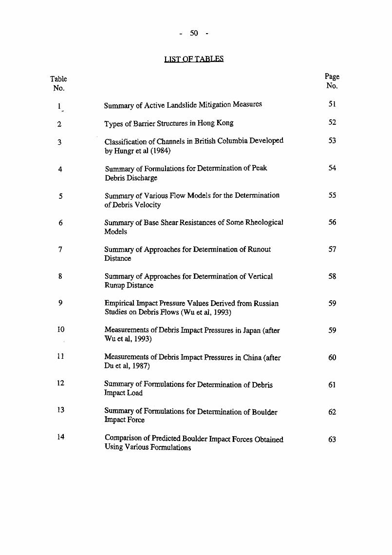
- 50

TJST OF TABLES

Table Page

No. No-

1 Summary of Active Landslide Mitigation Measures 51

2 Types of Barrier Structures in Hong Kong 52

3 Classification of Channels in British Columbia Developed 53byHungretal(1984)

4 Summary of Formulations for Determination of Peak 54Debris Discharge

5 Summary of Various Flow Models for the Determination 55of Debris Velocity

6 Summary of Base Shear Resistances of Some Rheological 56Models

7 Summary of Approaches for Determination of Runout 57Distance

8 Summary of Approaches for Determination of Vertical 58Runup Distance

9 Empirical Impact Pressure Values Derived from Russian 59Studies on Debris Flows (Wu et al, 1993)

10 Measurements of Debris Impact Pressures in Japan (after 59Wuetal, 1993)

11 Measurements of Debris Impact Pressures in China (after 60Duetal, 1987)

12 Summary of Formulations for Determination of Debris 61Impact Load

13 Summa^ 62Impact Force

14 Comparison of Predicted Boulder Impact Forces Obtained 63Using Various Formulations

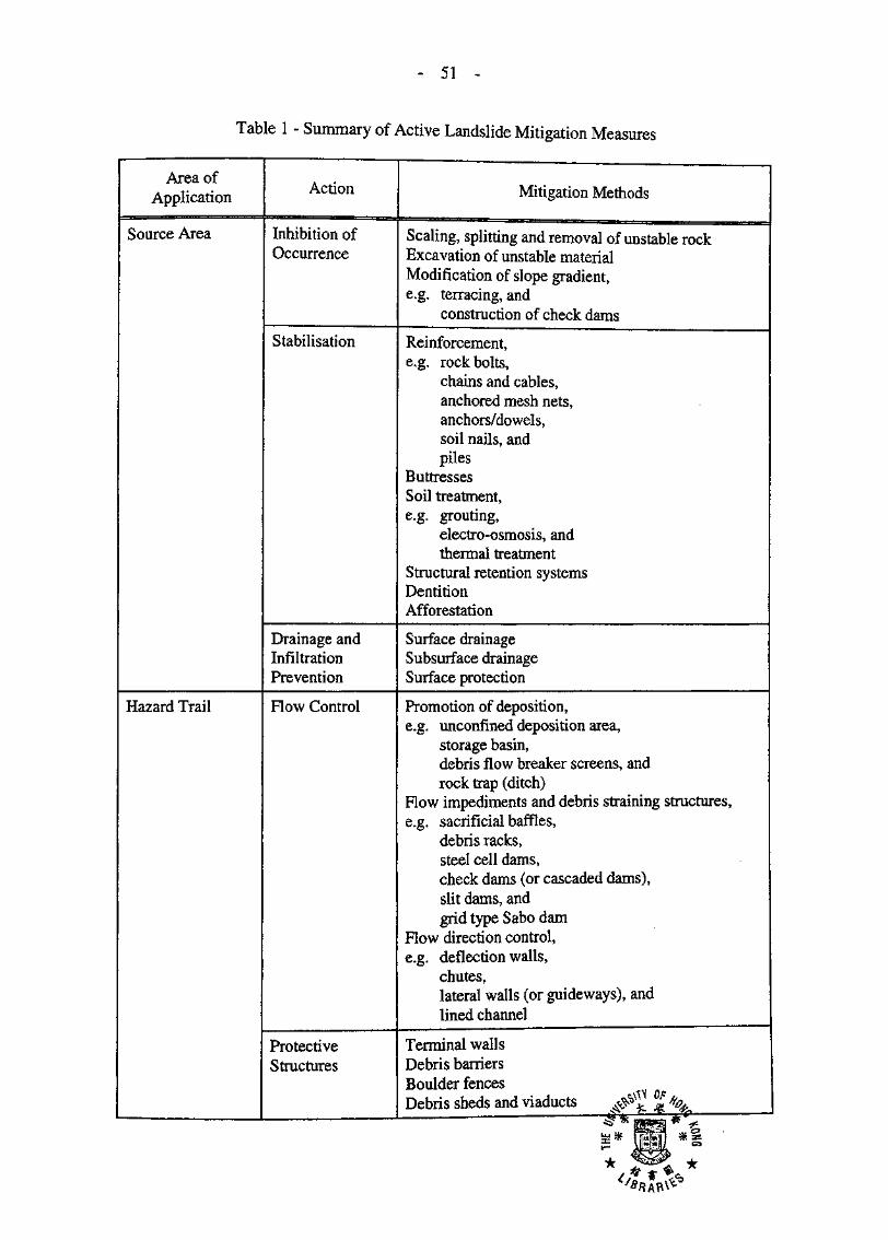
- 51

Table 1 - Summary of Active Landslide Mitigation Measures

Area ofApplication

Source Area

Hazard Trail

Action

Inhibition ofOccurrence

Stabilisation

Drainage andInfiltrationPrevention

Flow Control

ProtectiveStructures

Mitigation Methods

Scaling, splitting and removal of unstable rockExcavation of unstable materialModification of slope gradient,e.g. terracing, and

construction of check dams

Reinforcement,e.g. rock bolts,

chains and cables,anchored mesh nets,anchors/dowels,soil nails, andpiles

ButtressesSoil treatment,e.g. grouting,

electro-osmosis, andthermal treatment

Structural retention systemsDentitionAfforestation

Surface drainageSubsurface drainageSurface protection

Promotion of deposition,e.g. unconfined deposition area,

storage basin,debris flow breaker screens, androck trap (ditch)

Flow impediments and debris straining structures,e.g. sacrificial baffles,

debris racks,steel cell dams,check dams (or cascaded dams),slit dams, andgrid type Sabo dam

Flow direction control,e.g. deflection walls,

chutes,lateral walls (or guideways), andlined channel

Terminal wallsDebris barriersBoulder fencesDebris sheds and viaducts xjs*xl / %

— : : : : ' '. " " ~ . ^^IP^*"^

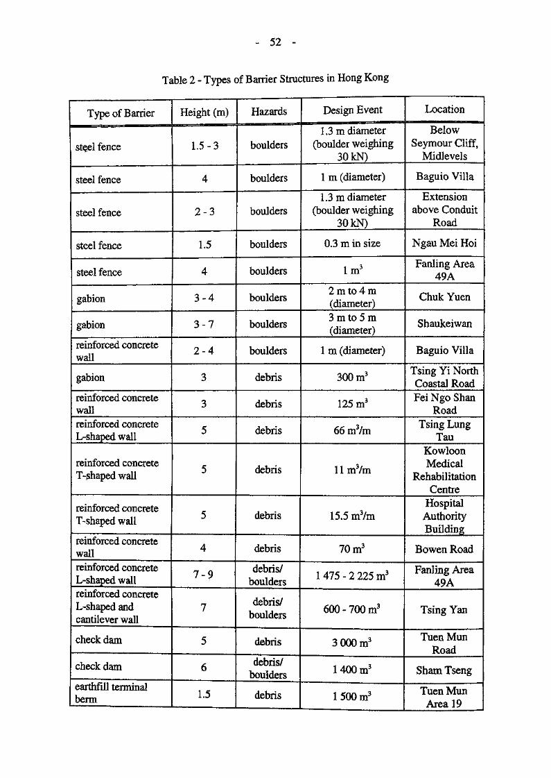
52

Table 2 - Types of Barrier Structures in Hong Kong

Type of Barrier

st^el fence

steel fence

steel fence

steel fence

steel fence

gabion

gabion

reinforced concretewall

gabion

reinforced concretewallreinforced concreteL-shapedwall

reinforced concreteT~$hapedwall

reinforced concreteT-shaped wall

reinforced concretewallreinforced concreteL~shaped wallreinforced concreteL-shapedandcantilever wall

check dam

check dam

earthfill terminalberm

Height (m)

L5-3

4

2-3

1.5

4

3-4

3-7

2-4

3

3

5

5

5

4

7-9

7

5

6

1.5

Hazards

boulders

boulders

boulders

boulders

boulders

boulders

boulders

boulders

debris

debris

debris

debris

debris

debris

debris/boulders

debris/boulders

debris

debris/boulders

debris

Design Event

1.3 m diameter(boulder weighing

30 kN)

1 m (diameter)

1.3 m diameter(boulder weighing

30 kN)

0.3 m in size

1m3

2 m to 4 m(diameter)3 m to 5 m(diameter)

1 m (diameter)

300m3

125m3

66 m3/m

l lmVm

15.5m3/m

70m3

1475-2225m3

600 - 700m3

3000m3

1400m3

1500m3

Location

BelowSeymour Cliff,

Midlevels

Baguio Villa

Extensionabove Conduit

Road

Ngau Mei Hoi

Fanling Area49A

Chuk Yuen

Shaukeiwan

Baguio Villa

Tsing Yi NorthCoastal RoadFei Ngo Shan

RoadTsing Lung

TauKowloonMedical

RehabilitationCentre

HospitalAuthorityBuilding

Bowen Road

Fanling Area49A

Tsing Yan

Tuen MunRoad

Sham Tseng

Tuen MunArea 19

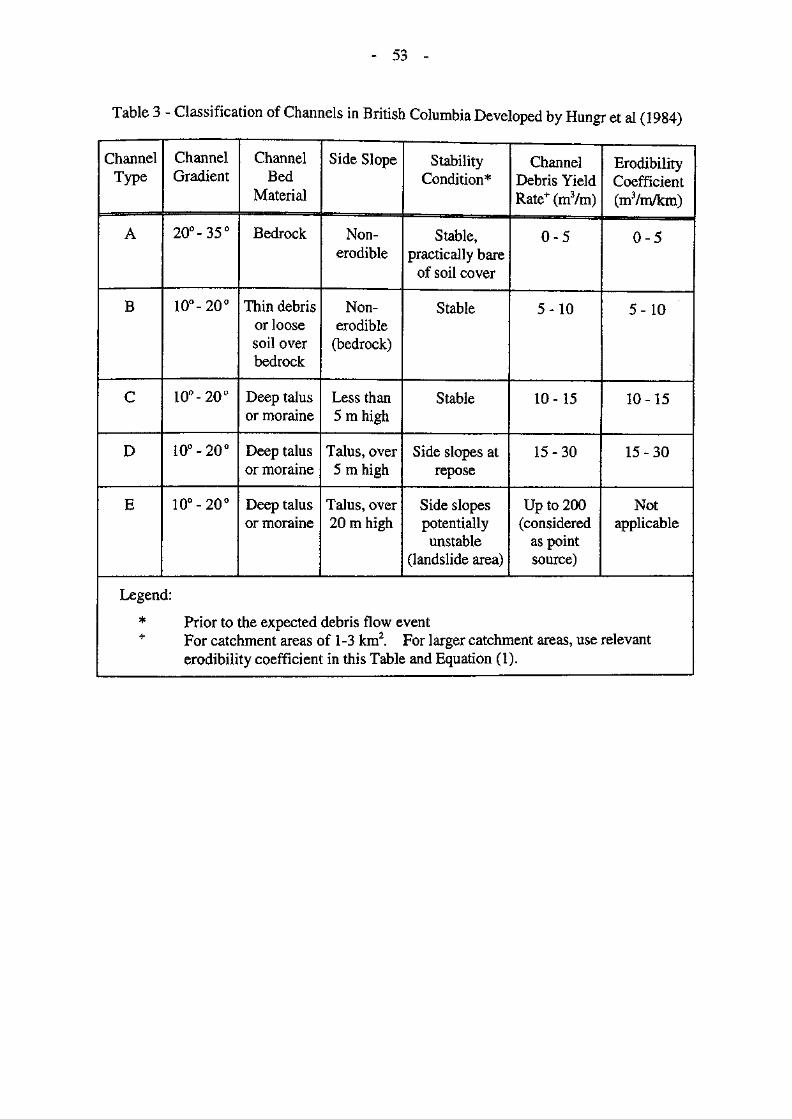
- 53 -

Table 3 - Classification of Channels in British Columbia Developed by Hungr et al (1984)

ChannelType

A

B

C

D

E

ChannelGradient

20° -35°

1Q°- 20°

10°- 20°

10° -20°

10° -20°

ChannelBed

Material

Bedrock

Thin debrisor loosesoil overbedrock

Deep talusor moraine

Deep talusor moraine

Deep talusor moraine

Side Slope

Non-erodible

Non-erodible

(bedrock)

Less than5 m high

Talus, over5 m high

Talus, over20 m high

StabilityCondition*

Stable,practically bare

of soil cover

Stable

Stable

Side slopes atrepose

Side slopespotentially

unstable(landslide area)

ChannelDebris YieldRate+ (mVm)

0-5

5-10

10-15

15-30

Up to 200(considered

as pointsource)

ErodibilityCoefficient(mVm/km)

0-5

5-10

10-15

15-30

Notapplicable

Legend:

* Prior to the expected debris flow event* For catchment areas of 1 -3 km2. For larger catchment areas, use relevant

erodibility coefficient in this Table and Equation (1).

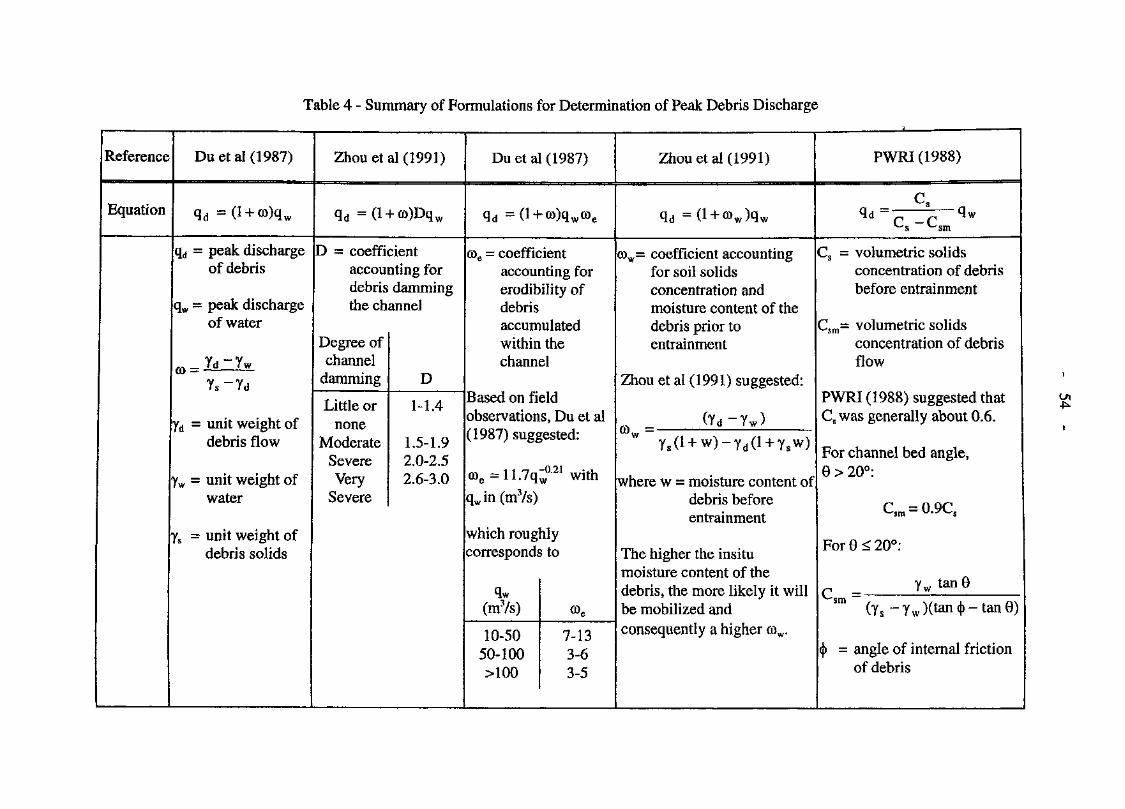
Table 4 - Summary of Formulations for Determination of Peak Debris Discharge

Reference

Equation

Duetal(1987)

qd =(l + co)qw

qd = peak dischargeof debris

qw = peak dischargeof water

co Y d ~ Y w

Ys-Yd

yd = unit weight ofdebris flow

yw = unit weight ofwater

ys = unit weight ofdebris solids

Zhou etal (1991)

qd -(l-hco)Dqw

D = coefficientaccounting fordebris dammingthe channel

Degree ofchannel

damming

Little ornone

ModerateSevereVery

Severe

D

1-1 4

1.5-1.92.0-2.52.6-3.0

Du etal (1987)

qd = (l-fco)qwG>e

coe = coefficientaccounting forerodibility ofdebrisaccumulatedwithin thechannel

Based on fieldobservations, Du et al(1987) suggested:

(De=11.7q^*21 withqwin(mVs)

which roughlycorresponds to

qw

(mVs)

10-5050-100>100

0>e

7-133-63-5

Zhou etal (1991)

qd -(l + o>w)qw

co w= coefficient accountingfor soil solidsconcentration andmoisture content of thedebris prior toentrainment

Zhou et al (1991) suggested:

Q _ ( Y d - Y w )Ys(l + w)-Yd( l + ysw)

where w = moisture content ofdebris beforeentrainment

The higher the insitumoisture content of thedebris, the more likely it willbe mobilized andconsequently a higher CDW.

PWRI(1988)

a Cs qq<* r p 3w^s ^sm

Cs = volumetric solidsconcentration of debrisbefore entrainment

Csm= volumetric solidsconcentration of debrisflow

PWRI (1988) suggested thatCs was generally about 0.6.

For channel bed angle,0 > 20°:

C = 0 . 9 C S

For 9 < 20°:

c Yw tan 6

(y s-Yw)( t an<l>- t an0)

<j> = angle of internal frictionof debris

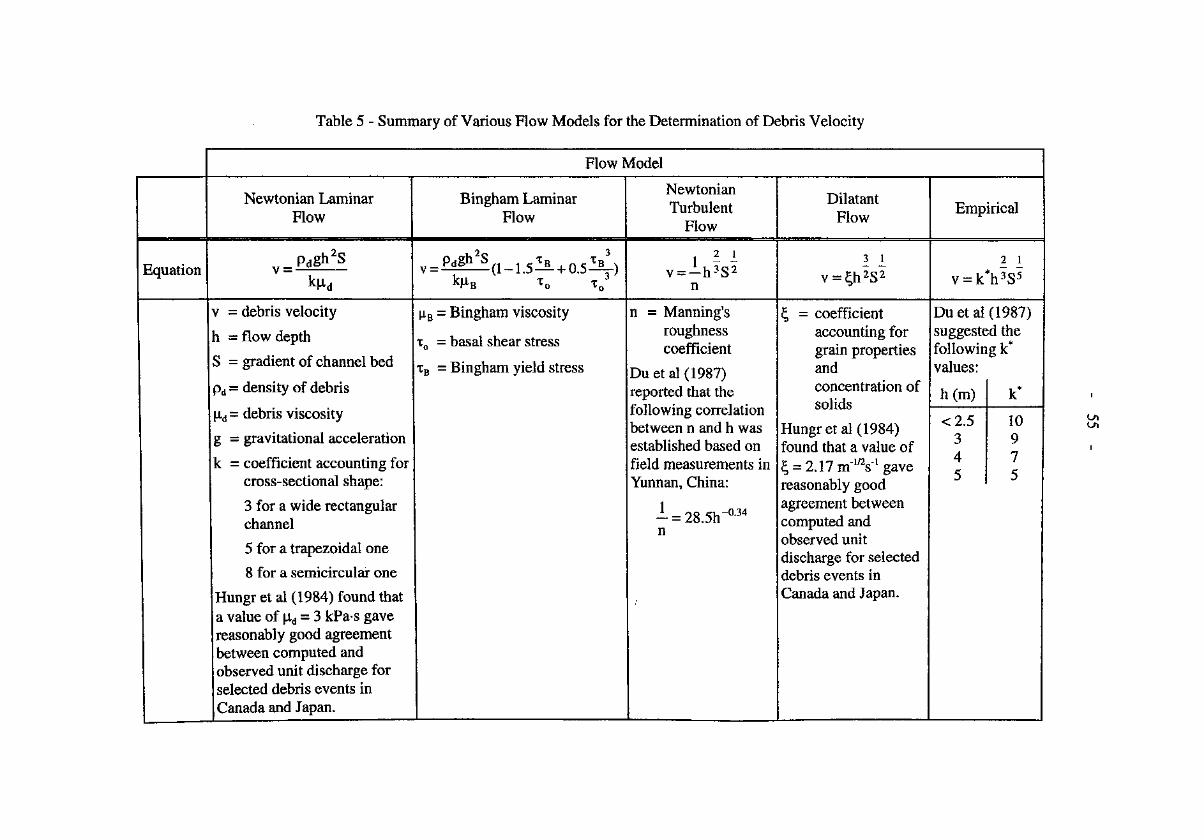
Table 5 - Summary of Various Flow Models for the Determination of Debris Velocity

Flow Model

Newtonian LaminarFlow

Bingham LaminarFlow

NewtonianTurbulent

Flow

DilatantFlow

Empirical

Equation2 1

n v = = k*h3S5

= debris velocity

= flow depth

= gradient of channel bed

pd = density of debris

|id= debris viscosity

g = gravitational acceleration

k = coefficient accounting forcross-sectional shape:

3 for a wide rectangularchannel

5 for a trapezoidal one

8 for a semicircular one

Hungr et al (1984) found thata value of \id = 3 kPa-s gavereasonably good agreementbetween computed andobserved unit discharge forselected debris events inCanada and Japan.

= Bingham viscosity

TO = basal shear stress

tB = Bingham yield stress

n = Manning'sroughnesscoefficient

Duetal(1987)reported that thefollowing correlationbetween n and h wasestablished based onfield measurements inYunnan, China:

~

^ = coefficientaccounting forgrain propertiesandconcentration ofsolids

Hungr etal (1984)found that a value of

reasonably goodagreement betweencomputed andobserved unitdischarge for selecteddebris events inCanada and Japan.

Duetal (1987)suggested thefollowing k*values:

Mm)

<2.5345

10975

(MUi

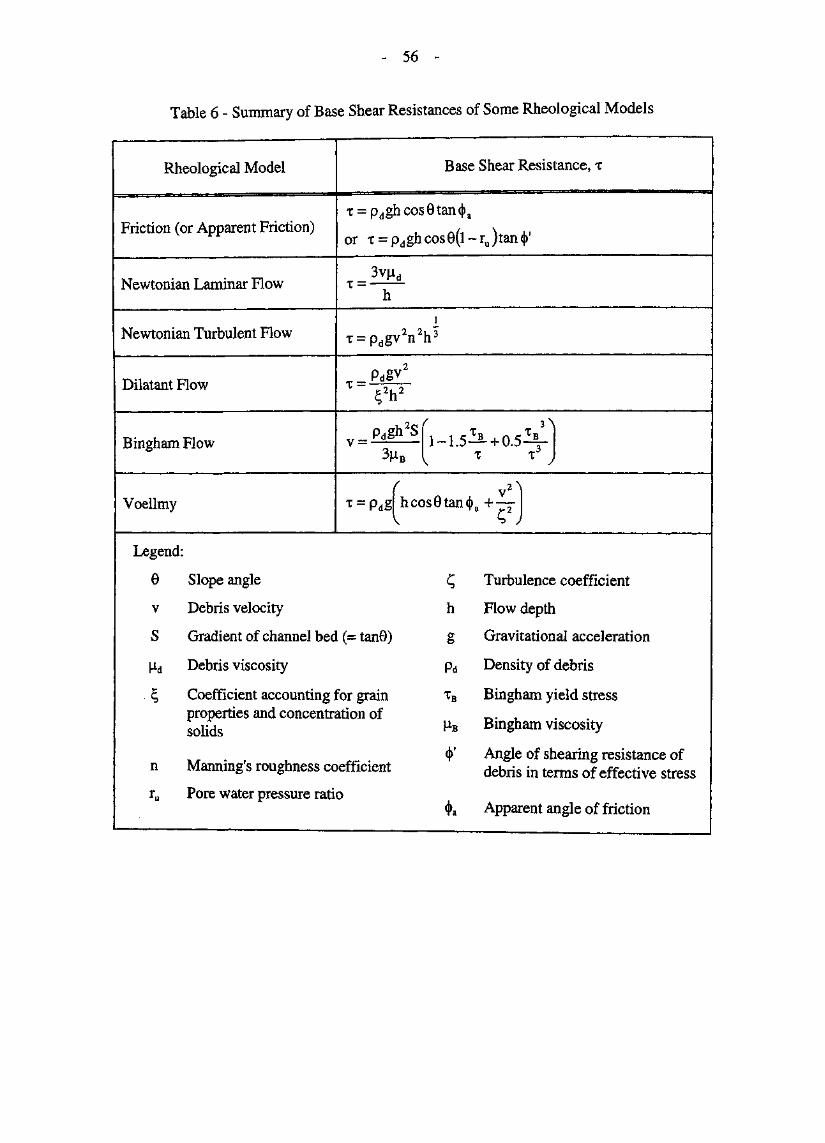
56

Table 6 - Summary of Base Shear Resistances of Some Rheological Models

Rheological Model Base Shear Resistance,

Friction (or Apparent Friction)t = pdghcos9tan<j)a

or T = pdghcos6(l~ru)tan<|)'

Newtonian Laminar Flow

Newtonian Turbulent Flow 2^2nV

Dilatant Flow T =pdg

y

Bingham How v =

Voellmy hcos6tan<|>a+ —V S >

Legend:

0 Slope angle

v Debris velocity

S Gradient of channel bed (= tanG)

|id Debris viscosity

^ Coefficient accounting for grainproperties and concentration ofsolids

n Manning's roughness coefficient

ru Pore water pressure ratio

£ Turbulence coefficient

h Flow depth

g Gravitational acceleration

pd Density of debris

TB Bingham yield stress

|LIB Bingham viscosity

•<j> ! Angle of shearing resistance ofdebris in terms of effective stress

<|>a Apparent angle of friction

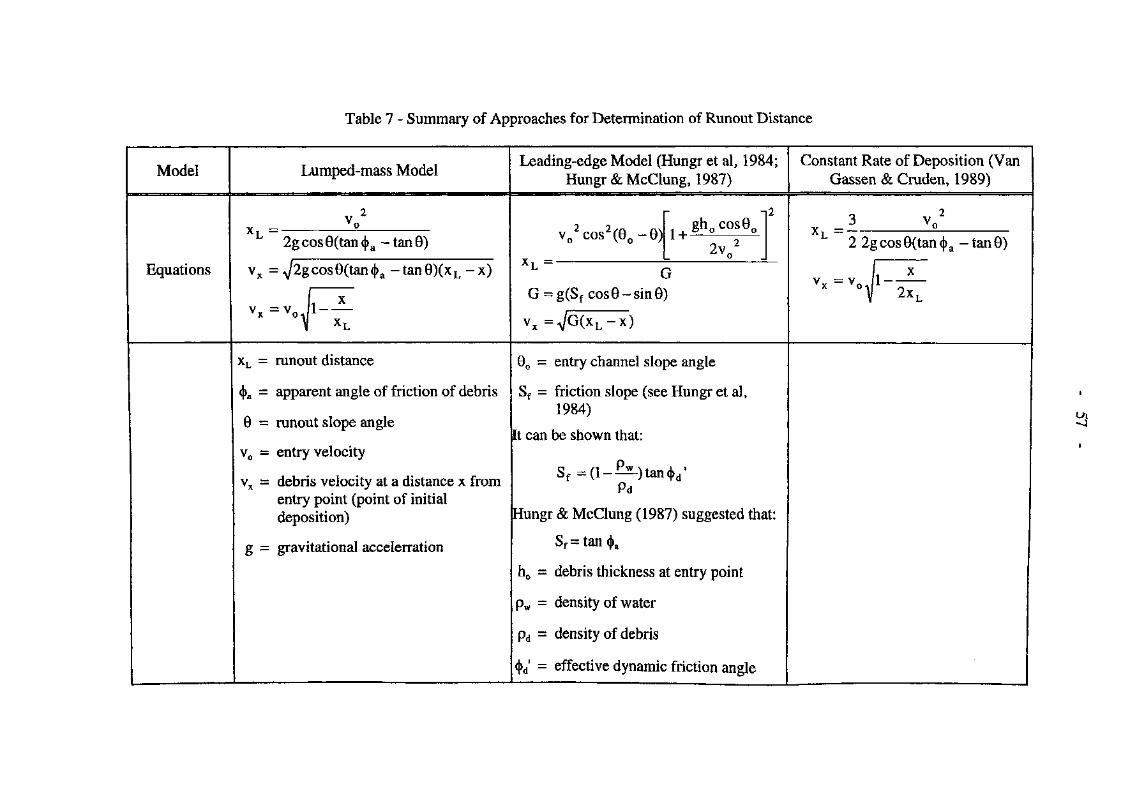
Table 7 - Summary of Approaches for Determination of Runout Distance

Model Lumped-mass ModelLeading-edge Model (Hungr et al, 1984;

Hungr & McClung, 1987)Constant Rate of Deposition (Van

Gassen & Craden, 1989)

Equations

2gcos9(tan<j>a -tan0)

vx = ̂ 2gcos0(tan <|>a — tan 0)(xL - x)

v x =v 0 J l - —XT

1+ gh0cos90 XL — —22gcos9(tan<j)a-tan9)

GG = g(Sf cos 0-sin 6)

1-2xL

vx =

XL = runout distance

^a = apparent angle of friction of debris

9 = runout slope angle

v0 = entry velocity

vx = debris velocity at a distance x fromentry point (point of initialdeposition)

g = gravitational acceleration

90 = entry channel slope angle

Sf = friction slope (see Hungr et al,1984)

It can be shown that:

Sf = ( i - . 2 LPd

Hungr & McClung (1987) suggested that:

Sf = tan<)>a

h0 = debris thickness at entry point

pw = density of water

pd = density of debris

^ = effective dynamic friction angle

Table 8 - Summary of Approaches for Determination of Vertical Runup Distance

Model Lumped-mass ModelLumped-mass Model Corrected

for Momentum Change(Perlaetal, 1980)

Leading-edge Model (Hungr & McClung,1987; Takahashi & Yoshida, 1979)

Equationv0 tan 9

2g(tan<|>a-htan9)0 2cos2(90+9)tan9

2g(tan(()a -Man 9)

_ v02cos2(90

g(tan<j>a+tan9)i gh0cos90

2 v '

Ah = runup distance

(j)a = apparent angle of friction of debris

9 = runup slope angle

vo = entry velocity

90 = entry channel slope angle h0 = approach debris thickness

Ul00

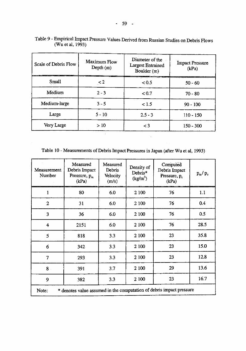
- 59

Table 9 - Empirical Impact Pressure Values Derived from Russian Studies on Debris Hows(Wuetal, 1993)

Scale of Debris Flow

Small

Medium

Medium-large

Large

Very Large

Maximum FlowDepth (m)

<2

2 - 3

3-5

5-10

>10

Diameter of theLargest Entrained

Boulder (m)

<0.5

<0.7

<1.5

2.5-3

<3

Impact Pressure(kPa)

50-60

70 - 80

90- 100

110-150

150-300

Table 10 - Measurements of Debris Impact Pressures in Japan (after Wu et al, 1993)

MeasurementNumber

1

2

3

4

5

6

7

8

9

MeasuredDebris ImpactPressure, pm

(kPa)

80

31

36

2151

818

342

293

391

382

MeasuredDebris

Velocity(m/s)

6.0

6.0

6.0

6.0

3.3

3.3

3.3

3.7

3.3

Density ofDebris*(kg/m3)

2100

2100

2100

2100

2100

2100

2 100

2100

2100

ComputedDebris ImpactPressure, pc

(kPa)

76

76

76

76

23

23

23

29

23

Pm/Pc

1.1

0.4

0.5

28.5

35.8

15.0

12.8

13.6

16.7

Note: * denotes value assumed in the computation of debris impact pressure

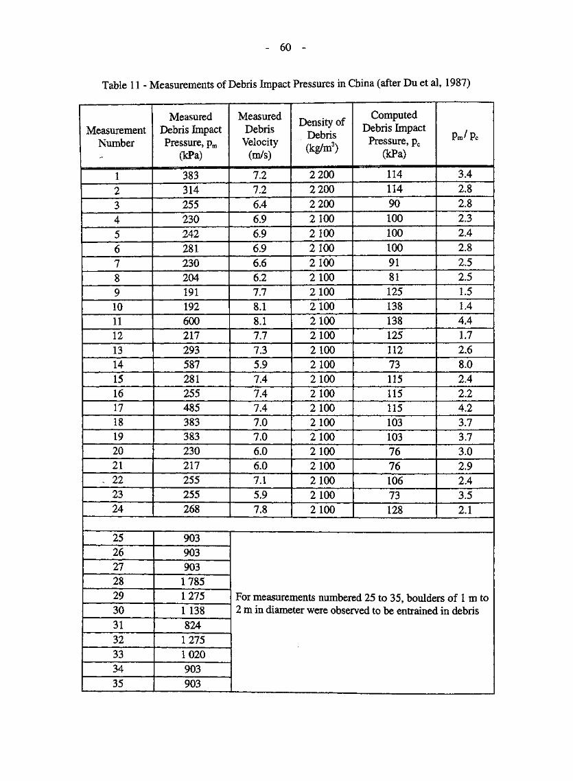
60 -

Table 11 - Measurements of Debris Impact Pressures in China (after Du et al, 1987)

MeasurementNumber

123456789101112131415161718192021

. 222324

MeasuredDebris ImpactPressure, pm

(kPa)

383314255230242281230204191192600217293587281255485383383230217255255268

MeasuredDebris

Velocity(m/s)

7.27.26.46.96.96.96.66.27.78.18.17.77.35.97.47.47.47.07.06.06.07.15.97.8

Density ofDebris(kg/m3)

220022002200210021002100210021002100210021002100210021002100210021002100210021002100210021002100

ComputedDebris Impact

Pressure, pc

(kPa)

11411490100100100

L 91

8112513813812511273115115115103103767610673128

Pm/Pc

3.42.82.82.32.42.82.52.51.51.44.41.72.68.02.42.24.23.73.73.02.92.43.52.1

2526272829303132333435

90390390317851 2751 138824

1 2751 020903903

For measurements numbered 25 to 35, boulders of 1 m to2 m in diameter were observed to be entrained in debris

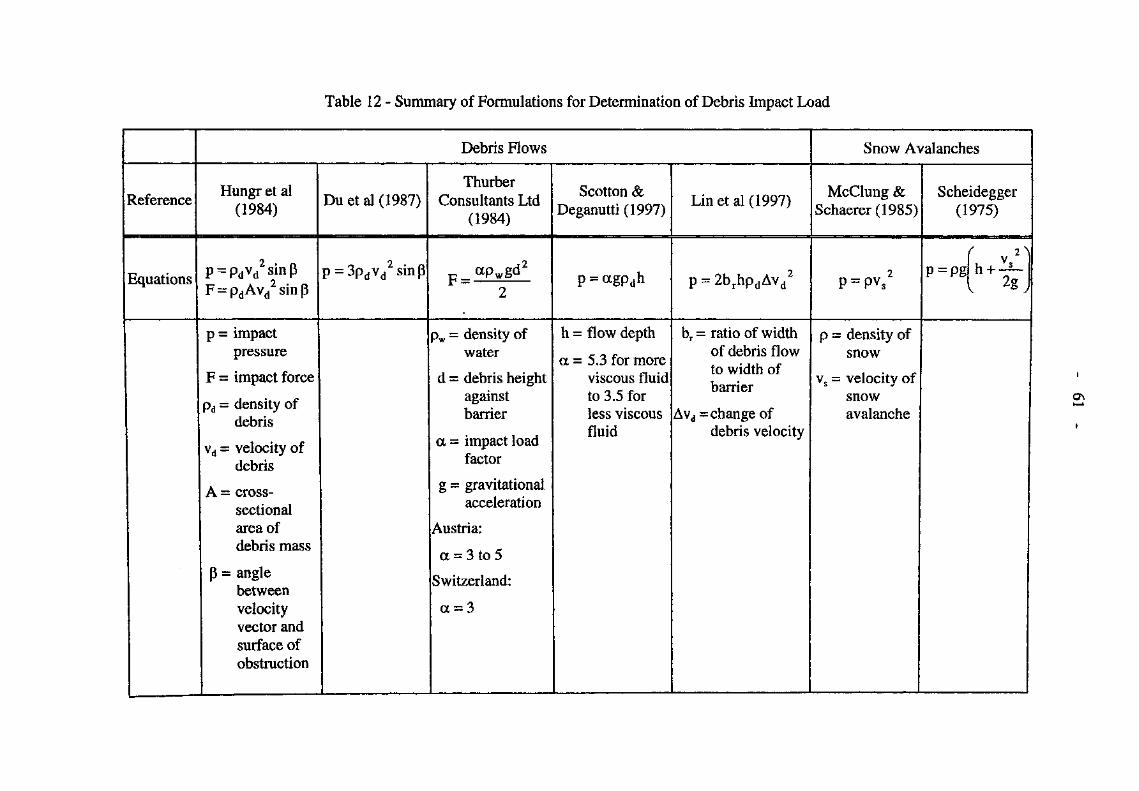
Table 12 - Summary of Formulations for Determination of Debris Impact Load

Reference

Equations

Debris Flows

Hungr et al(1984)

f\P PdVd S*nPF = pdAvd

2sinp

p = impactpressure

F = impact force

pd = density ofdebris

vd = velocity ofdebris

A = cross-sectionalarea ofdebris mass

P = anglebetweenvelocityvector andsurface ofobstruction

Duetal (19.87)

p-3pdvd smp

ThurberConsultants Ltd

(1984)

P <*pwgd2r — — "

2

pw = density ofwater

d = debris heightagainstbarrier

a = impact loadfactor

g = gravitationalacceleration

Austria:

a = 3 to 5

Switzerland:

a = 3

Scotton &Deganutti (1997)

P = «gpdh

h = flow depth

a = 5.3 for moreviscous fluidto 3.5 forless viscousfluid

Lin etal (1997)

p-2b rhpdAvd~

br = ratio of widthof debris flowto width ofbarrier

Avd= change ofdebris velocity

Snow Avalanches

McClung &Schaerer(1985)

P-pv s

p = density ofsnow

vs = velocity ofsnowavalanche

Scheidegger(1975)

r» r\rrl fi ! sp~pgr 2g j

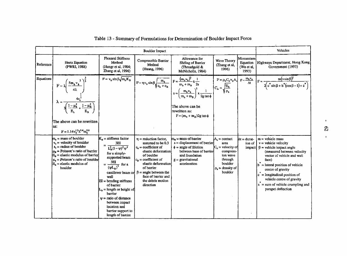
Table 13 - Summary of Formulations for Determination of Boulder Impact Force

Reference

Equations

Boulder Impact

Hertz Equation(PWRI,1988)

3

F i 1 b b j— A,j 1

I

/i-n2 i-nl^31 + I

V Eh EB /

The above can be rewrittenas:

m^ = mass of bouldervb = velocity of boulderrb - radius of boulderIB == Poisson's ratio of barrierSB = elastic modulus of barrierjjb = Poisson's ratio of boulderEj, - elastic modulus of

boulder

Flexural StiffhessMethod

(Hungr etal, 1984;Zhang etal, 1996)

F-vbsinp^Kj

KB = stiftness factor3EI

L3B(l-\j/)2\i/2

for a simply-supported beam

3Ctl _— "v tor a

(M/LB)3

cantilever beam orwall

El = bending stiffnessof barrier

Lg = length or height ofbarrier

vj/ = ratio of distancebetween impactlocation andbarrier support tolength of barrier

Compressible BarrierMethod

(Huang, 1996)

r^ —H"m V c b + c B

T| = reduction factor,assumed to be 03

cb = coefficient ofelastic deformationof boulder

CB = coefficient ofelastic deformationof barrier

p = angle between theface of barrier andthe debris motiondirection

Allowance forSliding of Barrier

(Threadgold&McMcholls, 1984)

Kvb)2 1m b - fmB 2s

S I I

The above can berewritten as:

F = (mh+mB)2gtan<|>

mB = mass of barriers = displacement of barrier$ = angle of friction

between base of barrierand foundation

g = gravitationalacceleration

Wave Theory(Zhang et al,

1996)

F = pbCbvbAc

C = (Ith 11• Ph

AC = contactarea

Cb — velocity orcompress-ion wavethroughboulder

Pt, = density ofboulder

MomentumEquation(Wu et al,

1993)

F_>hvbAt

At = durat-ion ofimpact

Vehicles

Highways Department, Hong KongGovernment (1993)

m(vsinp)2

m = vehicle massv = vehicle velocityP = vehicle impact angle

(measured between velocityvector of vehicle and wallface)

*b - lateral position of vehicle

centre of gravity*

c = longitudinal position ofvehicle centre of gravity

z = sum of vehicle crumpling andparapet deflection

ON

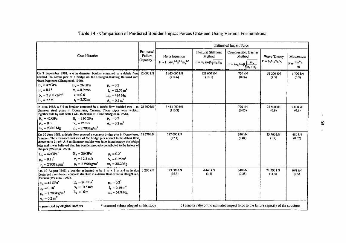
Table 14 - Comparison of Predicted Boulder Impact Forces Obtained Using Various Formulations

Case Histories

On 7 September 1981, a 6 m diameter boulder entrained in a debris flowsevered the centre pier of a bridge on the Chengdu-Kuming Railroad intothree fragments (Zhang et al, 1996).Eh=49GPa EB=26GPa m=0,2^h=0.i8 vh=8.9m/s I B = 12.56m4

pb = 2700kg/m3 M/ = (X6 mh = 414MgL B =22m rb = 3.32m Ac = 0,5m2

In June 1983, a 5,5 m boulder entrained in a debris flow buckled two I mdiameter steel pipes in Dongchuan, Yunnan. These pipes were weldedtogether side by side with a wall thickness of I cm (Zhang et al, 1996).Eb=42GPa EB = 210GPa Hb=0.2iiB=0.3 vb=12m/s Ac=0.2m2

mb = 230.6 Mg pb = 2700kg/m3

On 30 June 1981, a debris flow severed a concrete bridge pier in Dongchuan,Yunnan. The cross-sectional area of the bridge pier normal to the debris flowdirection is 21 m2. A 3 m diameter boulder was later found nearby the bridgejier and it was believed that this boulder probably contributed to the failure ofthe pier (Wuetal, 1993),

Eh = 42 GPa* EB = 26 GPa* |ih = 0,2*

^B=0,18* vl) = \2.5m/s Ac=0.25m2

pb = 2700 kg/m3 Pd = 2190 kg/m3 mh = 38.2Mg

On 10 August 1968, a boulder estimated to be 2 m x 3 m x 4 m in sizedestroyed a reinforced concrete structure in a debris flow event in DongchuanYunnan (Wuetal, 1993).Eb = 42GPa* EB = 26GPa* jab = 0.2*

^iB=0,18* vh = 10.5m/s I B = 0.16m4

ph = 2700kg/m3 L B =16m mh = 64.8Mg

Ac=0.2m2*

EstimatedFailure

Capacity -f

12000kN

28600kN

28770kN

1290kN

Estimated Impact Force

Hertz Equation

F = L14vbI2X(Umb

a6

2 623 GOO kN(218.6)

3 413 (XX) kN(119.3)

787 000 kN(27.4)

123 000 kN(95.3)

Flexural StiffnessMethod

F-v^inp^/n^K^

121 000 kN(10.1)

4440kN(3.4)

Compressible BarrierMethod

mF vnr ^tn R "-Tjvbsmp

V C b + C B

770 kN(0.06)

770 kN(0.03)

330 kN(0.01)

340 kN(0.26)

Wave TheoryF=p b C b v b A c

51 200 kN(4.3)

25 600 kN(0.9)

33300kN(1.2)

21 300 kN(16.5)

Momentum

F _ m h v bAt

3700kN(0.3)

2800kN(0.1)

480 kN(0.02)

648 kN(0.5)

+ provided by original authors * assumed values adopted in this study ( ) denotes ratio of the estimated impact force to the failure capacity of the structure

Chu>

- 64

T 1ST OF FIGURES

Figure Pa§e

No. No<

1 Possible Hazardous Scenarios Posed by Natural Hillside 66

2 Landslide Zones and Mechanisms of a Debris Flow (Franks 67& Woods, 1997)

3 Methods of Landslide Mitigation 68

4 Schematic Diagram Showing Some Active Mitigation 69Measures for Debris Flows

5 Construction of Site-specific Landsliding Frequency versus 70Source Volume Relationship (based on Tse et al, 1999)

6 Plot of Debris Volume versus Catchment Area 71

7 Peak Debris Flow Discharge versus Scale of Debris Flow 72(after Hungr et al, 1984; PWRI, 1988; Mizuyama et al,1992)

8 Debris Volume in Debris Flow Events in Val Varuna, 73Switzerland, 1772-1987 (after Davies, 1993)

9 Principles of the Sled Model 74

10 Flow Depth-Unit Discharge Relationships Predicted by 75Various Formulations

11 Classification of Debris Flow Events (after Kang et al, 761999)

12 Simulated and Observed Velocities for a Debris Flow Event 77in Kamikamihori Valley (Rickenmann & Koch, 1997)

13 Source Volume versus Apparent Angle of Friction 78Correlation for Open Hillside Failures (Ayotte & Hungr,1998)

14 Schematic of Runup Process Assumed by Different Models 79

15 Comparison of Computed and Measured Debris Impact 80Pressures

65 -

Figure PageNo. No.

16 Comparison of Apparent Angle of Friction Used in DAN 81Analysis with Observed Travel Angle of Debris

17 Data on Debris Mobility for Different Mechanisms and 82Scales of Natural Terrain Landslides in Hong Kong

18 Comparison of Data Extracted from DAN Analysis with 83Those Predicted by Flow Models

19 Maximum Debris Frontal Velocity and Debris Thickness 84Corresponding to the Four Debris Volume Ranges

20 Comparison of Measured and Computed Vertical Runup 85Distances Using Various Models

21 Suggestions for Assessment of Debris Mobility and Debris 86Impact Loading

22 Some Typical Decanting or Straining Structures (Czerny, 871998)

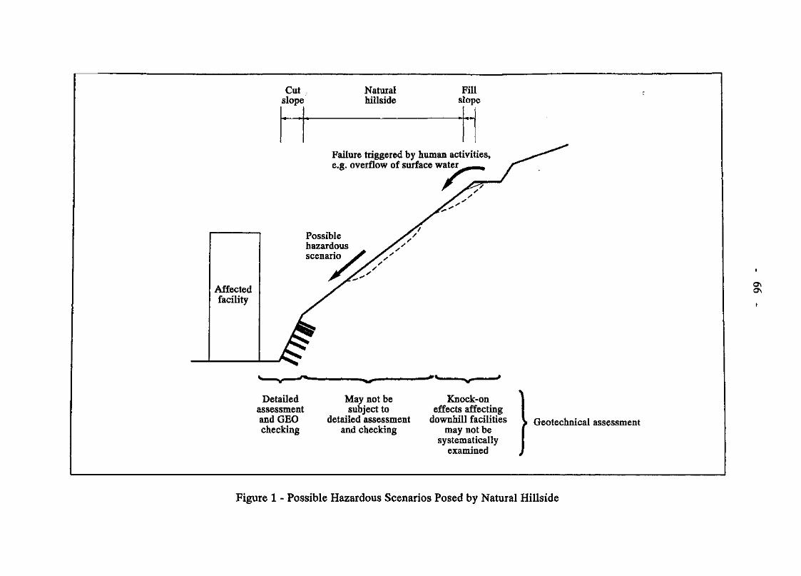
Cutslope

Naturalhillside

Fillslope

Failure triggered by human activities,e.g. overflow of surface water

Affectedfacility

Possiblehazardousscenario

Os

i

Detailedassessmentand GEOchecking

May not besubject to

detailed assessmentand checking

Knock-oneffects affecting

downhill facilitiesmay not be

systematicallyexamined

Geotechnical assessment

Figure 1 - Possible Hazardous Scenarios Posed by Natural Hillside

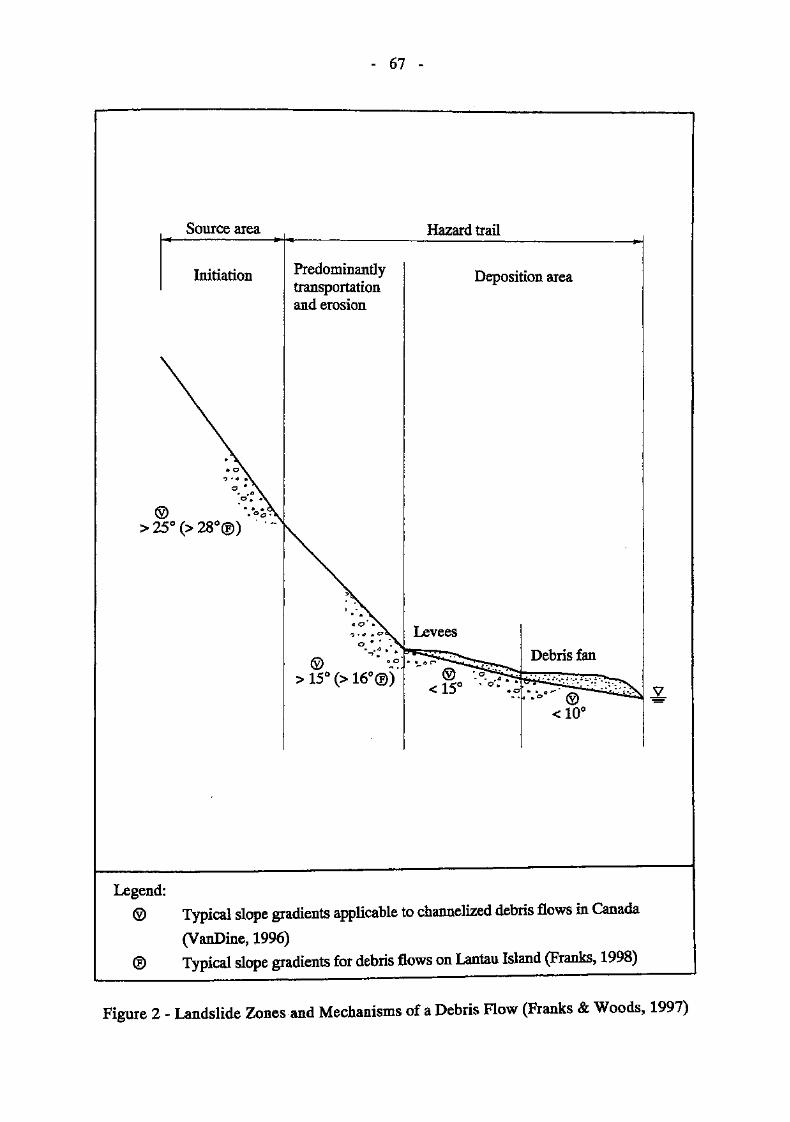
67 -

Source area

Initiation

> 25° (> 28

Hazard trail

Predominantlytransportationand erosion

> 15° (> 16v

Legend:Typical slope gradients applicable to channelized debris flows in Canada

(VanDine, 1996)Typical slope gradients for debris flows on Lantau Island (Franks, 1998)

Figure 2 - Landslide Zones and Mechanisms of a Debris Flow (Franks & Woods, 1997)

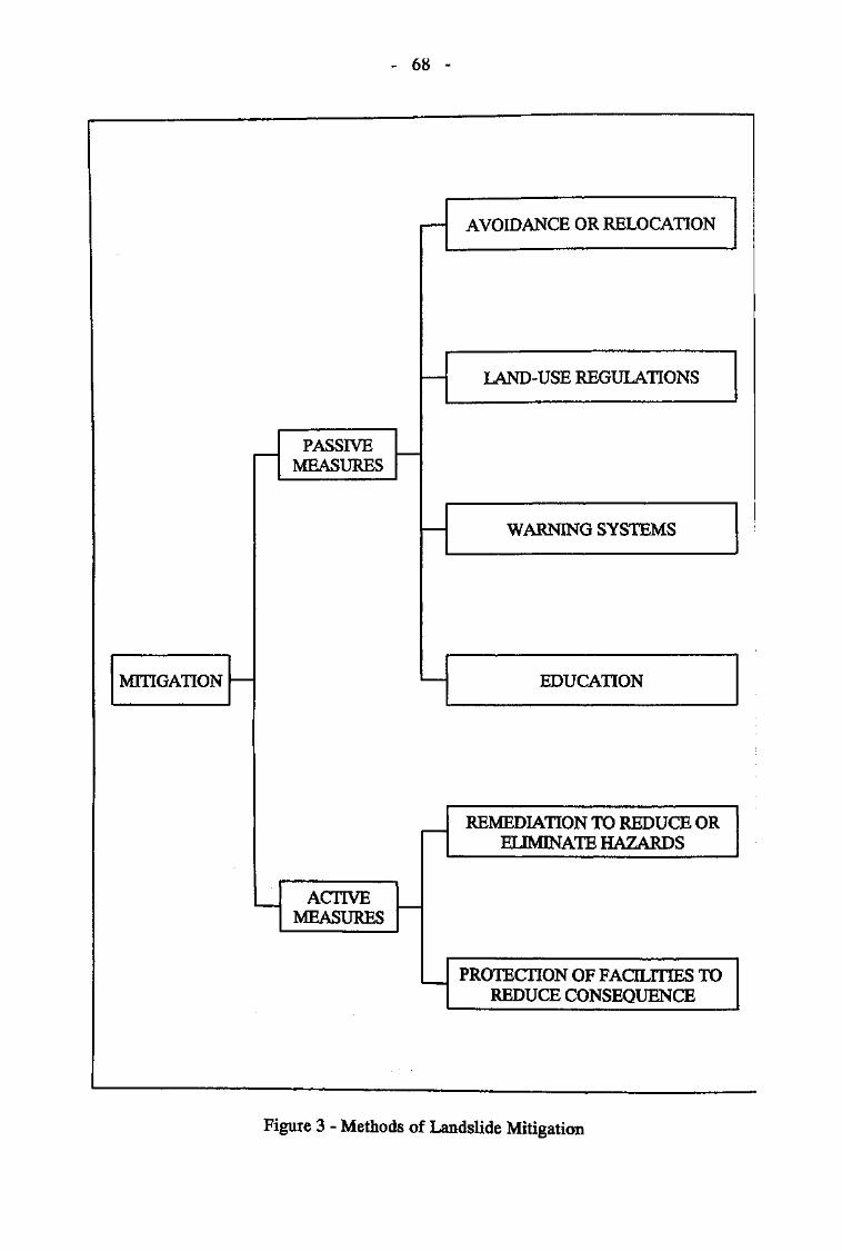
MITIGATION

PASSIVEMEASURES

AVOIDANCE OR RELOCATION

LAND-USE REGULATIONS

WARNING SYSTEMS

EDUCATION

ACTIVEMEASURES

REMEDIATION TO REDUCE ORELIMINATE HAZARDS

PROTECTION OF FACILITIES TOREDUCE CONSEQUENCE

Figure 3 - Methods of Landslide Mitigation

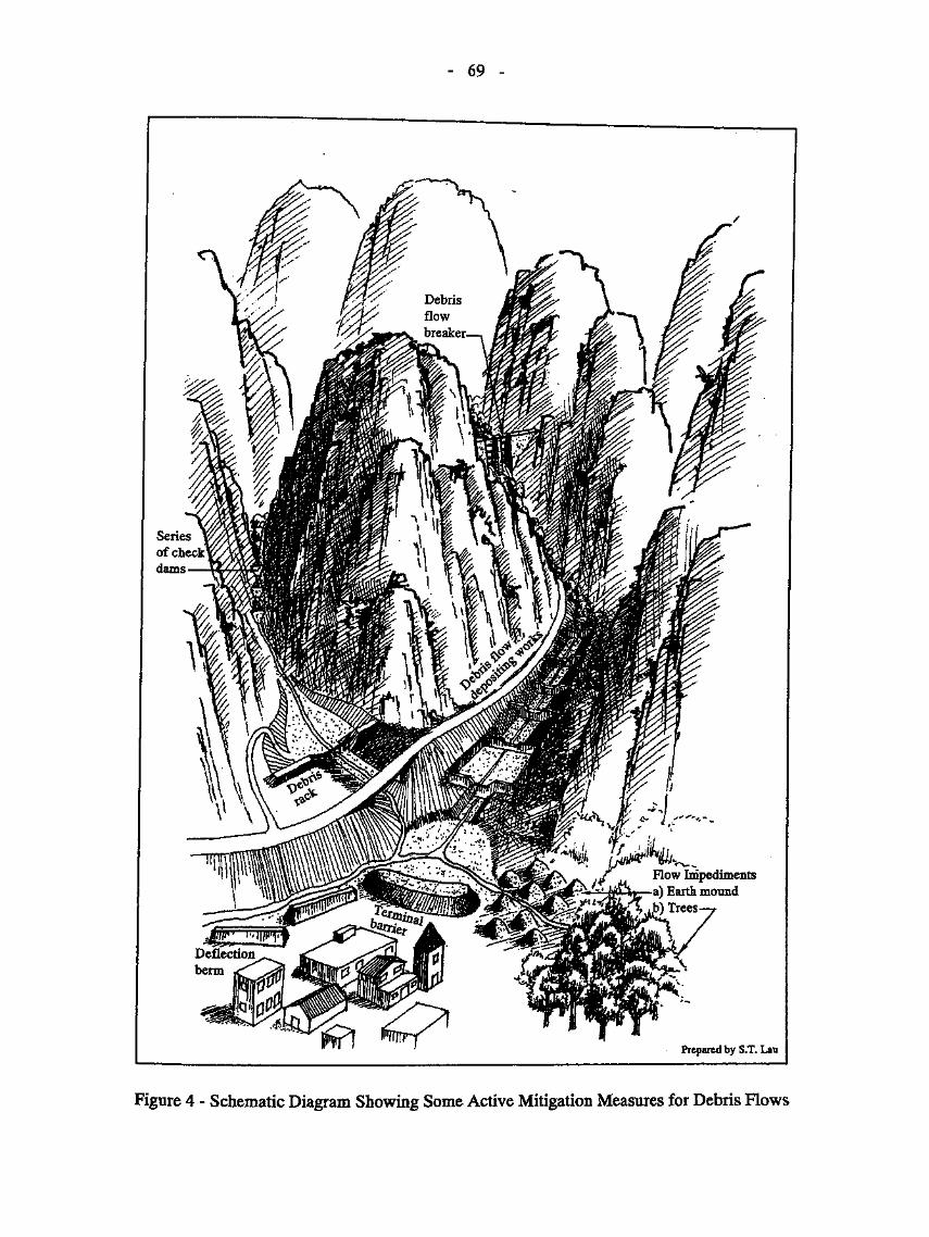
- 69 -

Seriesof checkdams

ents

Prepared by S.T. Lau

Figure 4 - Schematic Diagram Showing Some Active Mitigation Measures for Debris Flows

- 70 -

Site-specific curve forrecent landslides(frequency on annual basis)

Slope parallel to thoseof Wong et al & Franks

0.00110 100 1000 10000

Landslide Volume at Source, V (m3)

Legend:

Failures on open hillsides (based on Wong et al, 1998)Failures adjacent to streamcourses (based on Wong et al, 1998)Failures on open hillsides and adjacent to streamcourses(based on Wong et al, 1998)Failures documented in a landslide study on Lantau (based on Franks, 1998)Site-specific curve from API (based on recent and relict landslides)Site-specific curve from API (based on recent landslides)

Figure 5 - Construction of Site-specific Landsliding Frequency versus Source VolumeRelationship (based on Tse et al, 1999)

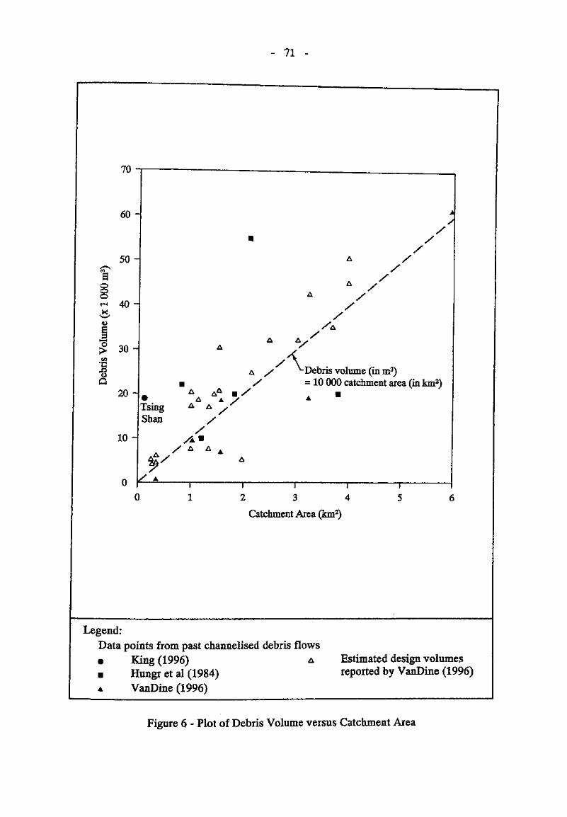
- 71 -

70

60 -

50 -

40 -

30 -

2<DQ

20 -

10 -

A ATsing A A ̂Shan /

/

/ A A A

A &

XA X Debris volume (in m3)/ =10 000 catchment area (in km2)

I

32 3 4

Catchment Area (km2)

Legend:Data points from past channelised debris flows• King (1996) A• Hungr et al (1984)A VanDine (1996)

Estimated design volumesreported by VanDine (1996)

Figure 6 - Plot of Debris Volume versus Catchment Area

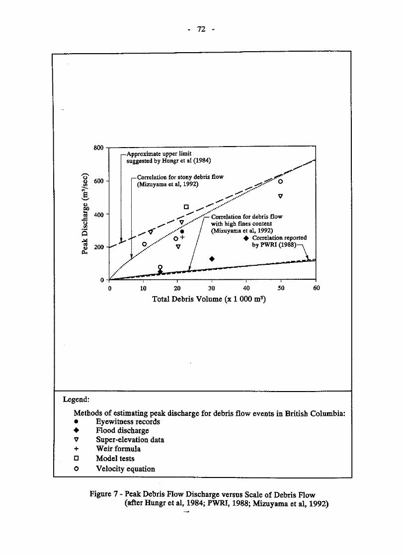
- 72 -

800-Approximate upper limitsuggested by Hungr et al (1984)

-Correlation for stony debris flow(Mizuyama et al, 1992)

Correlation for debris flowwith high fines content(Mizuyama et al, 1992)

Correlation reportedby PWRI (1988)-

10 20 30 40

Total Debris Volume (x 1 000 m3)

Legend:

Methods of estimating peak discharge for debris flow events in British Columbia:• Eyewitness records+ Flood dischargev Super-elevation data

.+. ' Weir formulaD Model testso Velocity equation

Figure 7 - Peak Debris Flow Discharge versus Scale of Debris Flow(after Hungr et al, 1984; PWRI, 1988; Mizuyama et al, 1992)

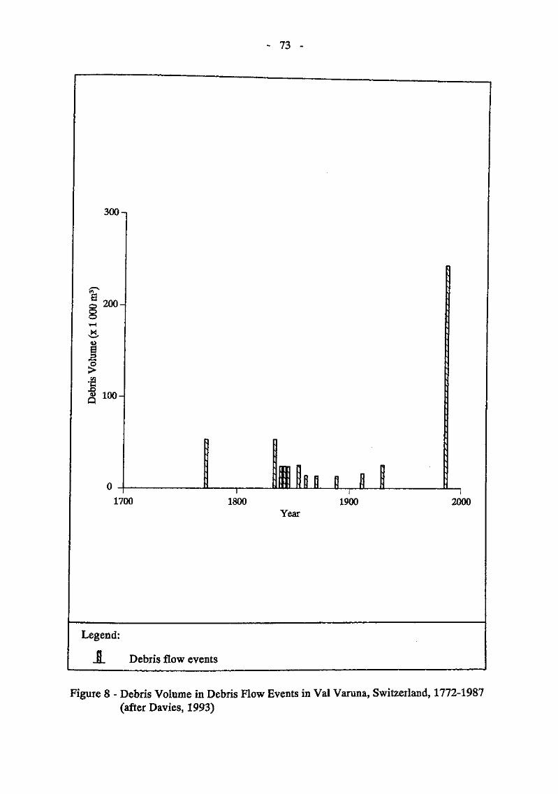
- 73 -

300-,

200-

1700

f i n1800 1900 2000

Year

Legend;

JL Debris flow events

Figure 8 - Debris Volume in Debris Flow Events in Val Varuna, Switzerland, 1772-1987(after Davies, 1993)

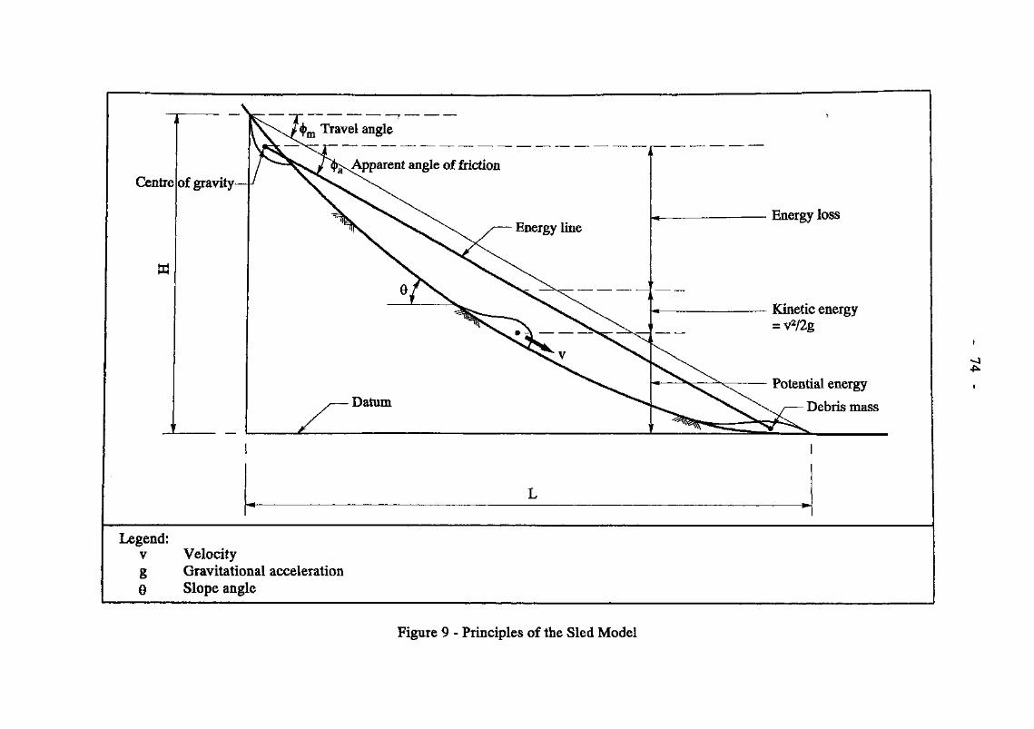
Centre of gravity—

rm Travel angle

Apparent angle of friction

Energy lineEnergy loss

Kinetic energy= v2/2g

Potential energy

Debris mass

Legend:v Velocityg Gravitational acceleration8 Slope angle

Figure 9 - Principles of the Sled Model

1000

o•s

100 r

4

r•8ca

10 r

1 r

0,1

Flow Depth (m)

Legend:Newtonian laminar flow ( nd = 3kPa« s)Dilatant flow ( £ = 2.17 m112 s'1)Newtonian turbulent flow (1/n = 28.5 h"°'34)Inclination of channel bed

Empirical formula (from Du et al, 1987)Canadian data (from Hungr et al, 1984)Japanese data (from Hungr et al, 1984)

Figure 10 - Flow Depth-Unit Discharge Relationships Predicted by Various Formulations

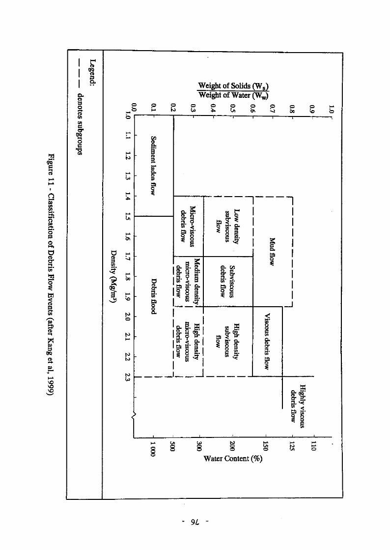
1a>i~*H^

Q

o"

o*po

OCDcr3.CA

a1

SEf

CDP

OP

sovo

1 ff1 crq

01 P

1 *CLOp0r-t-Oc/»C/>

crOQ

o

C/3

Weight of Solids (Ws)Weight of Water (Ww)

P p p p p p o p o o H-*M° h* • IO W 4X Ui ON ^ bo \O O

b

H*

Mto

H*

W

M

'"*

M

tJ\

h-»>

O H.s ^00

^ ^1 *P H^

OJ vo

to*o

to*~*

toto

toOi

1 ' . i , i " —i— r- 1

f r ' • • ' • • ' • ' • ' ' ' ' ' ' ' ' : ' '

y ' - " ' ' ' ' ' " • • • ' • ' • ' ' ' •

" 1o» . . . . :o

p)j HJj

H* Os- ^& oS*

^ |WJ

B ^g^ 1 &

Q k«K H*» f^,

55" ^N c ^BJ fe ^"a

^ ill5a <j CL

^ 8 ft-g ̂

n nS cVCT 3?!

c? |- cu^ O M

g 4" 1 s1 a

CL (/I

8-s-M« "^

II<! c«

§* qcTO «' CL

^ 8 I£ S2.1/3 ^>^

J

.a

f

i5s.

GO

o*a*CO*

C?

^

||

> i3!'^ §«

,§ 0 0 o o u\ o

° Water Content (%)

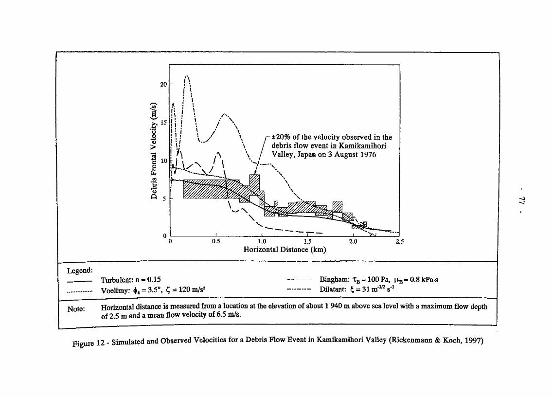
20

^i*\5Q

1̂•̂

*15*1-Koo•—<4)>

- T 3i10feO5

«r-iM•s

. 0 5

n

A.' -,i \.

4 ' *** *

!i !i i !I "• |« I J\ * ,

i-'lh\d..\UtX>_.._ir — •

~t\

XN' / \v / \V •' ^\ s *^*.*^ ,

\1^ ^

<V \--v — .1...%f%%%ZZ%2%%^,,wMMmmfamm^m^m^Af f S f s r f f S f f f f f f f K f s s f ^ p ^

/

±20% of the velocity observed in thedebris flow event in Kamikamihori

m̂w,7w**

/»»

w-y\

I\ "^vja^^v

\

Valley, Japan on 3

"\\\\\

%'V— ,'&$&zMi!^s%uV?77&&P~^^ '&&'&

August 1976

^-̂ -̂ .X..

0f

0.5f 1

1.0 1.5

Wk\^<s^Vsq

r̂ ::; r̂̂ B!:"--2.0 2.5

Horizontal Distance (km)

Legend:Turbulent: n = 0.15Vnellmv* d> - 3 5°, C

— — - Bingham: TB = 100 Pa, fiB = 0.8 kPa-s= 120 m/s2

Note: Horizontal distance is measured from a location

Dilatant: 4 = 31m"1/2s-1

at the elevation of about 1 940 m above sea level with a maximum flow depthof 2.5 ni and a mean flow velocity of 6.5 m/s.

Figure 12 - Simulated and Observed Velocities for a Debris Flow Event in Kamikamihori Valley (Rickenmann & Koch, 1997)

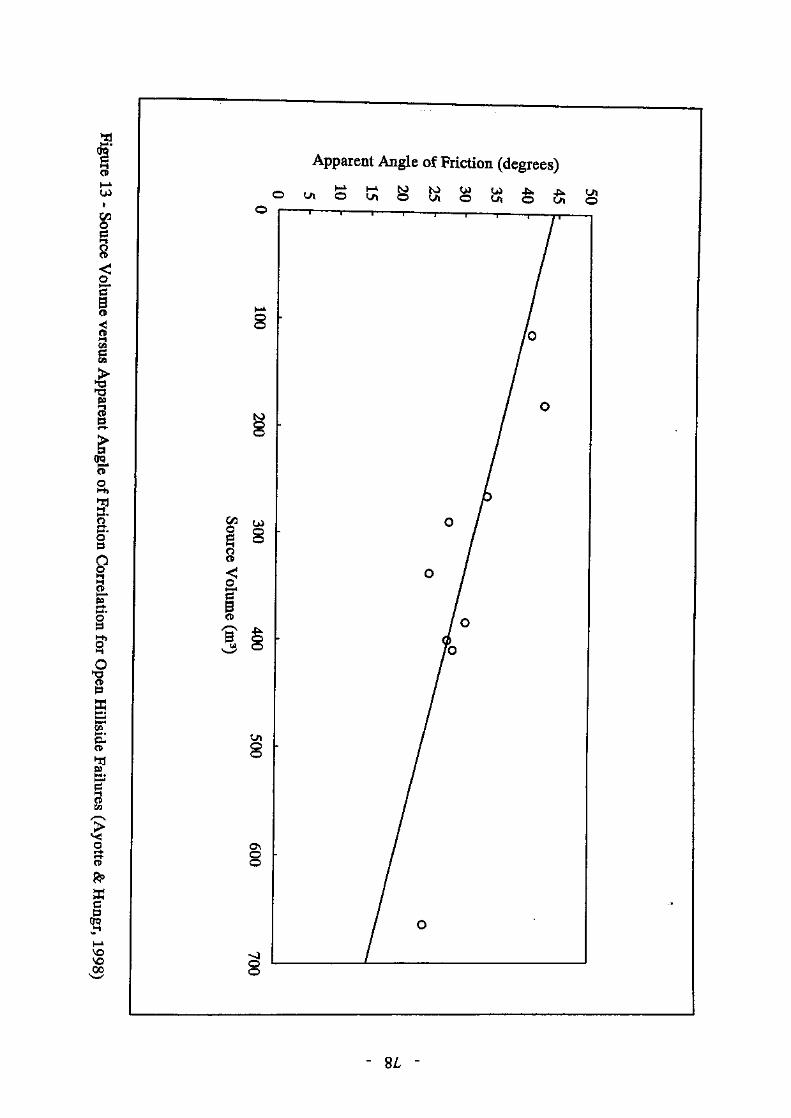
C/3O

8

II

§p

o

&.o

JL

o*

pffi

LO

MjCOM^»

$oO3

fO

DCTQ

Apparent Angle of Friction (degrees)

- 8Z, -

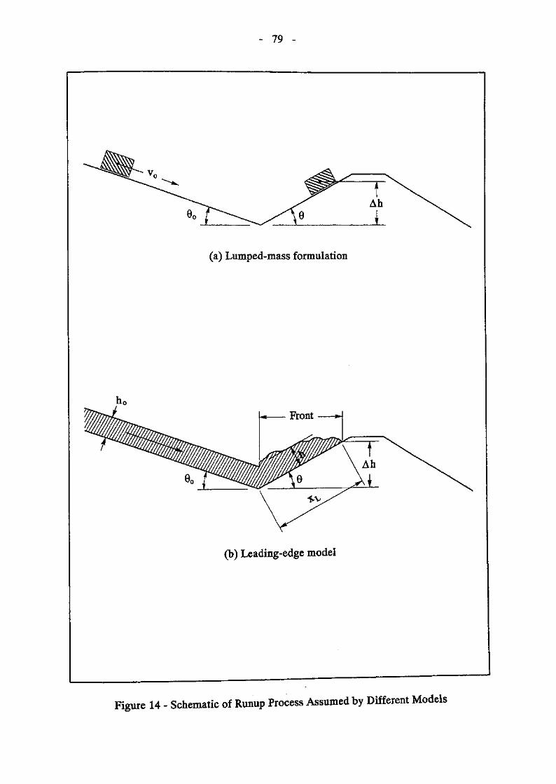
- 79 -

(a) Lumped-mass formulation

(b) Leading-edge model

Figure 14 - Schematic of Runup Process Assumed by Different Models

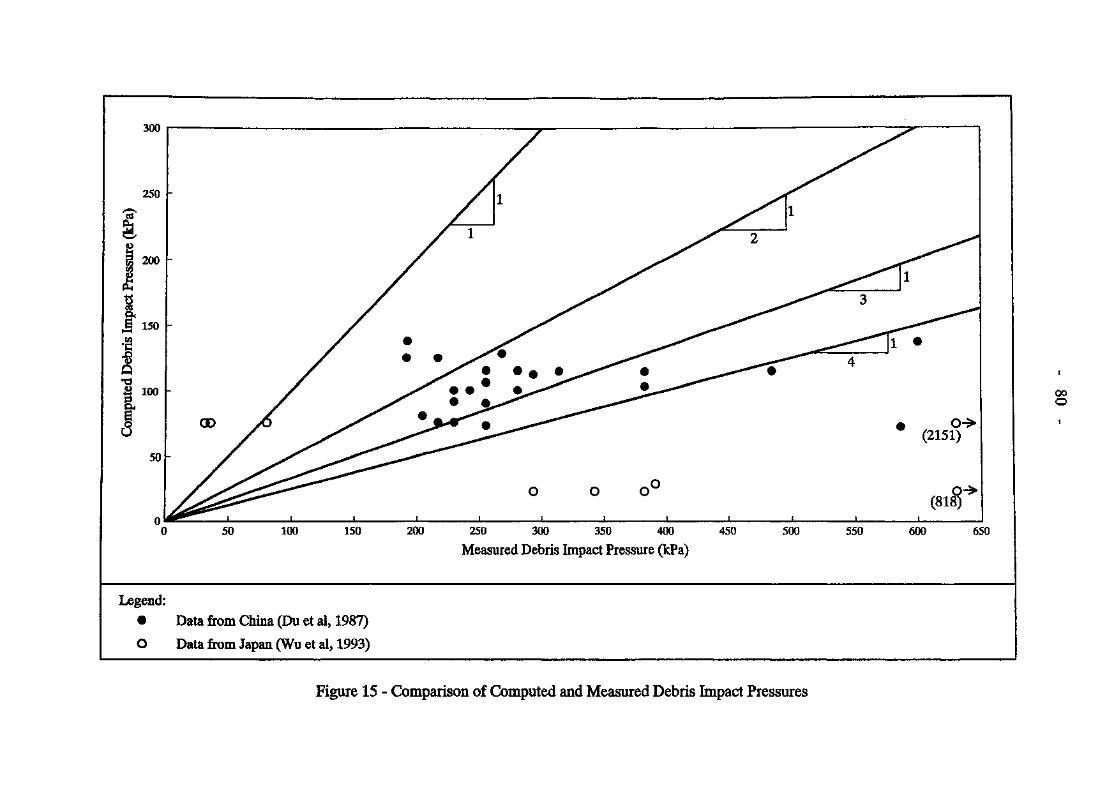
0 50 100 200 250 300 350 400

Measured Debris Impact Pressure (kPa)

ooo

450 500 550 600 650

Legend:• Data from China (Du et al, 1987)

O Data from Japan (Wu et al, 1993)

Figure 15 - Comparison of Computed and Measured Debris Impact Pressures

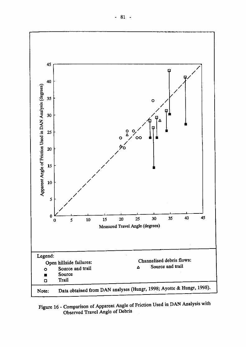
- 81 -

45

40

aO

t35

30

fi.9 25"2

VD

P

§ 20

o<L>

g 10S3

O O/A /

O / OO

. /

/

/

10 15 20 25 30 35

Measured Travel Angle (degrees)

/

40 45

Legend:Open hillside failures:o Source and trail• SourceD Trail

Channelised debris flows:A Source and trail

Note: Data obtained from DAN analyses (Hungr, 1998; Ayotte & Hungr, 199

Figure 16 - Comparison of Apparent Angle of Friction Used in DAN Analysis withObserved Travel Angle of Debris

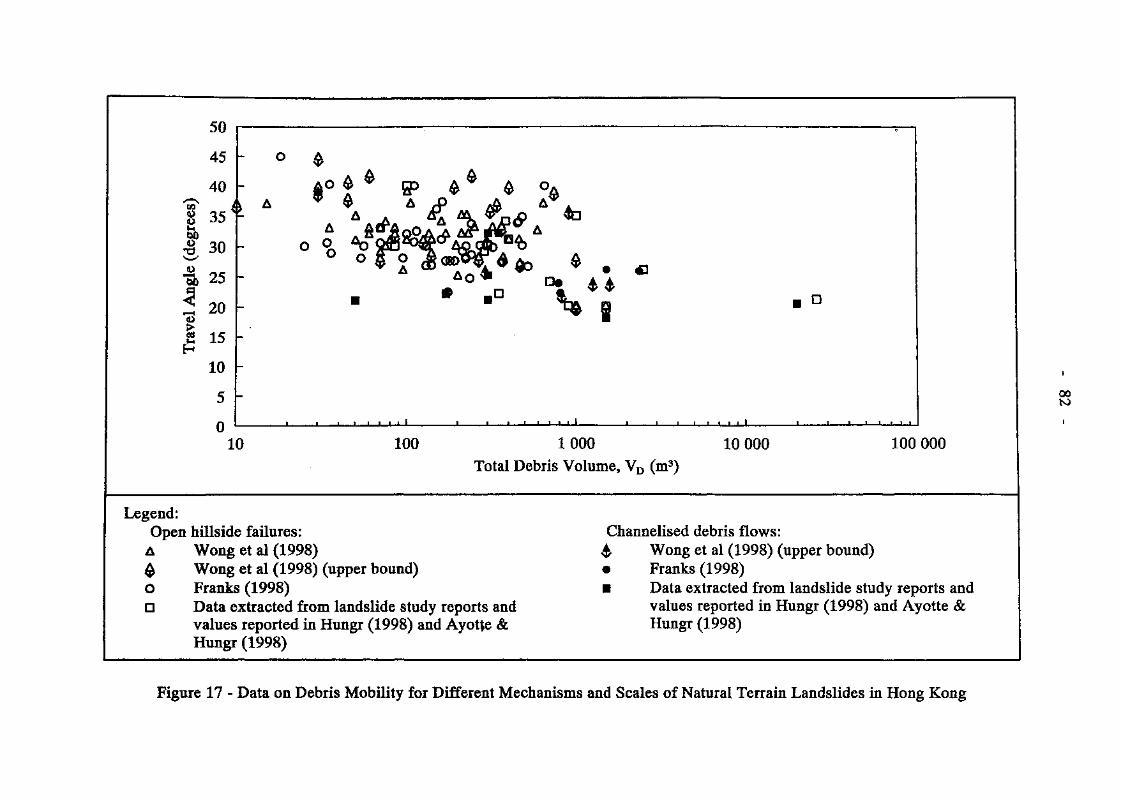
50

45

40

| 35

I! 30

.•§> 25

I 20

I 15

10

5

010

00to

100 1000Total Debris Volume, VD (m3)

10000 100000

Legend:Open hillside failures:

A Wong et al (1998)$ Wong et al (1998) (upper bound)o Franks (1998)D Data extracted from landslide study reports and

values reported in Hungr (1998) and Ayotte &Hungr (1998)

Channelised debris flows:4 Wong et al (1998) (upper bound)• Franks(1998)• Data extracted from landslide study reports and

values reported in Hungr (1998) and Ayotte &Hungr (1998)

Figure 17 - Data on Debris Mobility for Different Mechanisms and Scales of Natural Terrain Landslides in Hong Kong

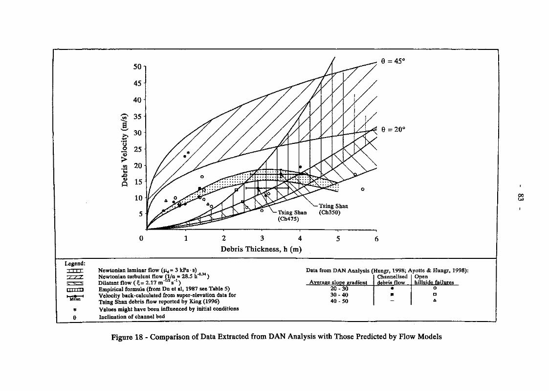
8 =45°

0

e =20°

oo

2 3 4Debris Thickness, h (m)

Legend;Newtonian laminar flow (nd - 3 kPa * s)Newtonian turbulent flow (1/n = 28.5 h~°*34)Dilatant flow ( £= 2.17 mr'V1)Empkical formula (from Du et al, 1987 see Table 5)Velocity back-calculated from super-elevation data forTsing Shan debris flow reported by King (1996)Values might have been influenced by initial conditionsInclination of channel bed

Data from DAN Analysis (Hungr, 1998; Ayotte & Hungr, 1998):

Average slope gradient20-3030-4040 - 50

Channeliseddebris flow

••

Openhillside failures

oDA

Figure 18 - Comparison of Data Extracted from DAN Analysis with Those Predicted by Flow Models

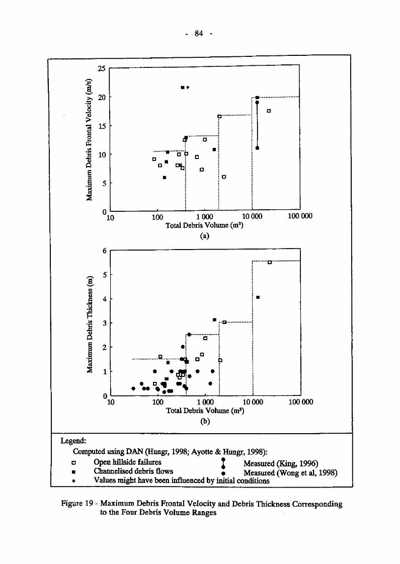
ty (

m/

tO O

Deb

ris

Fron

tal

H*

H-*

O

Ui

10

ckne

ss (m

Deb

ris

10

- 84 -

a-

if a"

a

0

100 1000 10000Total Debris Volume (m3)

(a)

100000

• am ••• %*w

a•

-Q--

..... —or ...... .........

100 1000 10000Total Debris Volume (m3)

(b)

100000

Legend:Computed using DAN (Hungr, 1998; Ayotte & Hungr, 1998):a Open hillside failures J Measured (King, 1996)• Channelised debris flows « Measured (Wong et al, 1998)* Values might have been influenced by initial conditions

Figure 19 - Maximum Debris Frontal Velocity and Debris Thickness Correspondingto the Four Debris Volume Ranges

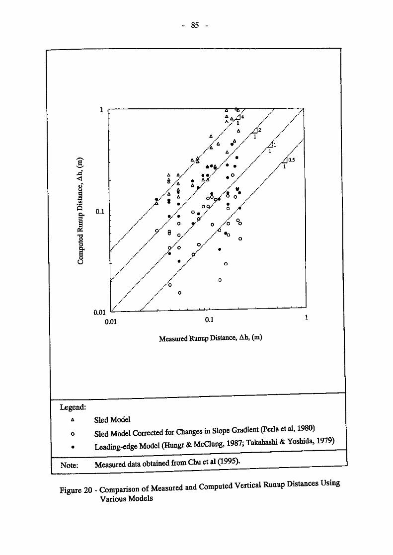
-c

8

.23Q

1!

0.010.01

- 85 -

A A

• ;

9''/•

^Zi4k X 1

®

A / / 1

r / §0oo^"'''8 o*

°*x* o ,/1 • /P*' / o

!•' O X*O ^

/ -b oox"

0.1

Measured Runup Distance, Ah, (m)

/]0.5

Legend:

A Sled Model

Sled Model Corrected for Changes in Slope Gradient (Perla et al, 1980)

. Leading-edge Model (Hungr & McClung, 1987; Takahashi & Yoshida, 1979)

Note: Measured data obtained from Chu et al (1995).

Figure 20 - Comparison of Measured and Computed Vertical Runup Distances Using

Various Models

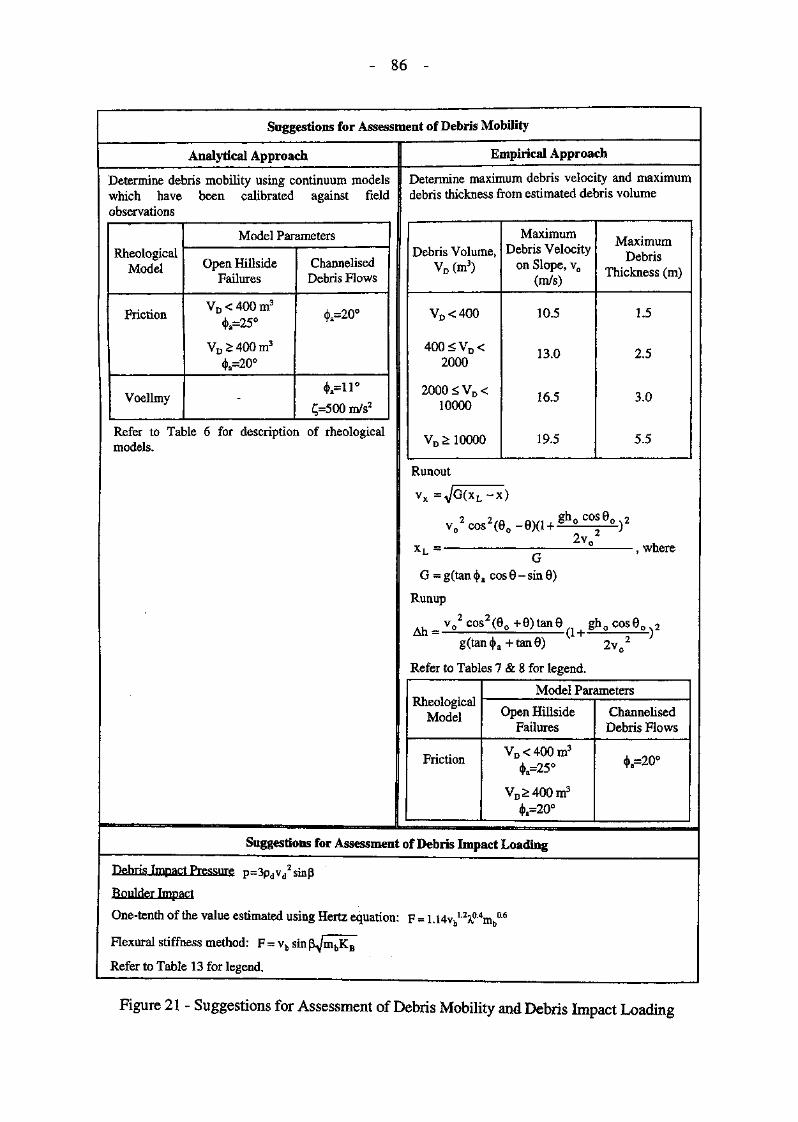
- 86

Suggestions for Assessment of Debris Mobility

Analytical Approach Empirical Approach

Determine debris mobility using continuum modelswhich have been calibrated against fieldobservations

RheologicalModel

Friction

Voellmy

Model Parameters

Open HillsideFailures

VD<400m3

(|>a=25*

VD > 400 m3

<|>a=200

-

ChannelisedDebris Flows

<t»a=20°

^=n°C=500 m/s2

Refer to Table 6 for description of rheologicalmodels.

Determine maximum debris velocity and maximumdebris thickness from estimated debris volume

Debris Volume,VD (m3)

VD<400

400<VD<2000

2000 < VD <10000

VD£ 10000

MaximumDebris Velocity

on Slope, v0

(m/s)

10.5

13.0

16.5

19.5

MaximumDebris

Thickness (m)

1.5

2.5

3.0

5.5

Runout

GG = g(tan (|)a cos 0 - sin 0)

Runup

Ah=-

• , where

gh 0cos0 0 . 2

g(tant|)a+tan0)

Refer to Tables 7 & 8 for legend.

RheologicalModel

Friction

Model Parameters

Open HillsideFailures

VD<400m3

VD>400m3

<|>a=200

ChannelisedDebris Flows

4>a=20°

Suggestions for Assessment of Debris Impact Loading

Debris Impact Pressure p=3pdvd2sinp

Boulder Impact

One-tenth of the value estimated using Hertz equation: F = 1.14vb12X0-4mb°'6

Flexural stiffness method: F = vh sin S-/mKKRO ~ \ D B

Refer to Table 13 for legend.

Figure 21 - Suggestions for Assessment of Debris Mobility and Debris Impact Loading

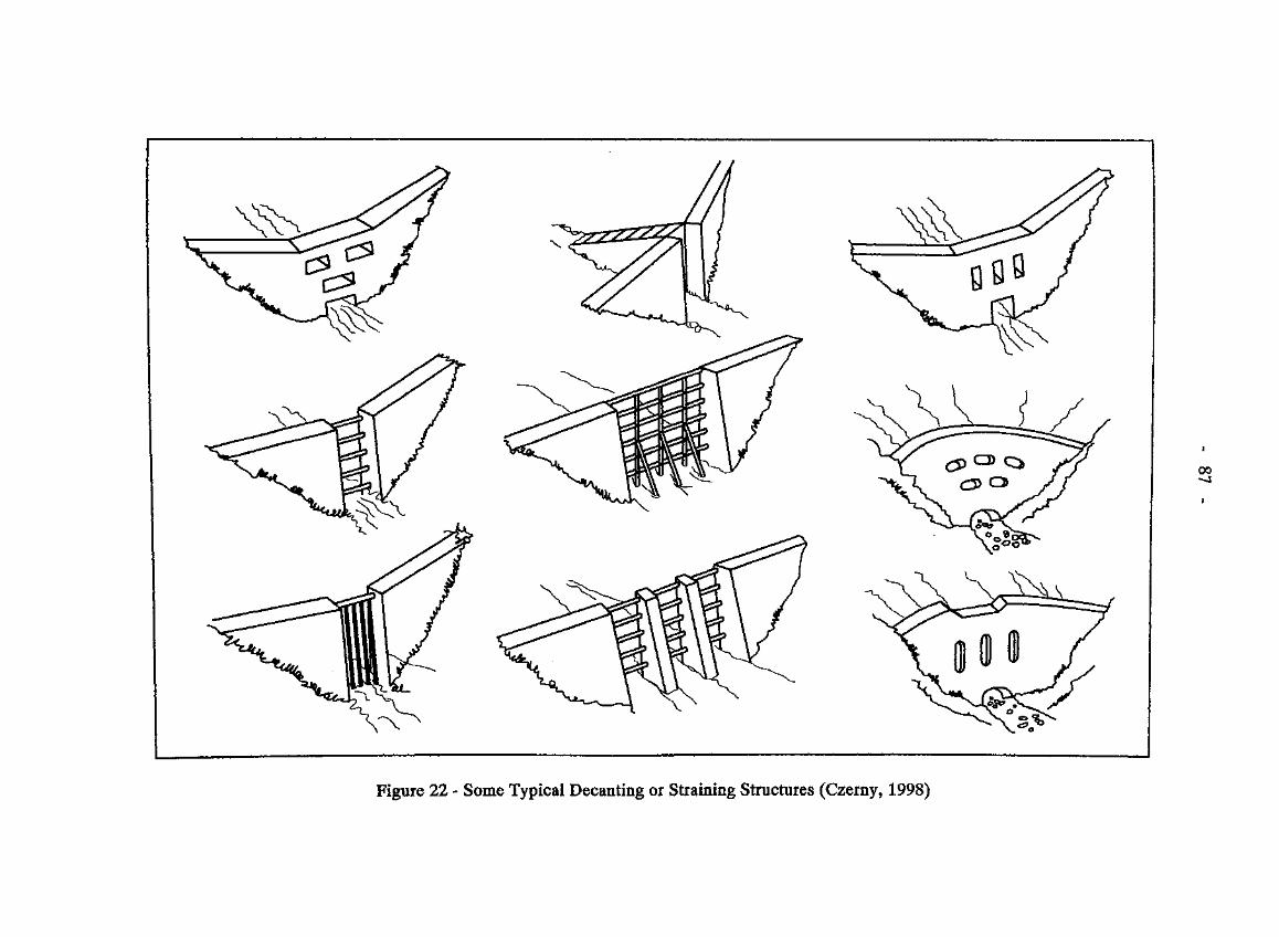
00

Figure 22 - Some Typical Decanting or Straining Structures (Czerny, 1998)

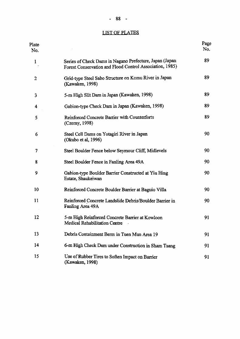
LIST OF PLATES

Plate PageNo. No-

1 Series of Check Dams in Nagano Prefecture, Japan (Japan 89Forest Conservation and Flood Control Association, 1985)

2 Grid-type Steel Sabo Structure on Komu River in Japan 89(Kawaken, 1998)

3 5-m. High Slit Dam in Japan (Kawaken, 1998) 89

4 Gabion-type Check Dam in Japan (Kawaken, 1998) 89

5 Reinforced Concrete Barrier with Counterforts 89(Czerny, 1998)

6 Steel Cell Dams on Yotagiri River in Japan 90(Okuboetal?1996)

7 Steel Boulder Fence below Seymour Cliff, Midlevels 90

8 Steel Boulder Fence in Fading Area 49A 90

9 Gabion-type Boulder Barrier Constructed at Yiu Hing 90Estate, Shaukeiwan

10 Reinforced Concrete Boulder Barrier at Baguio Villa 90

11 Reinforced Concrete Landslide Debris/Boulder Barrier in 90Fanling Area 49A

12 5-m High Reinforced Concrete Barrier at Kowloon 91Medical Rehabilitation Centre

13 Debris Containment Berm in TuenMun Area 19 91

14 6^m High Check Dam under Construction in Sham Tsang 91

15 Use of Rubber Tires to Soften Impact on Barrier 91(Kawaken, 1998)

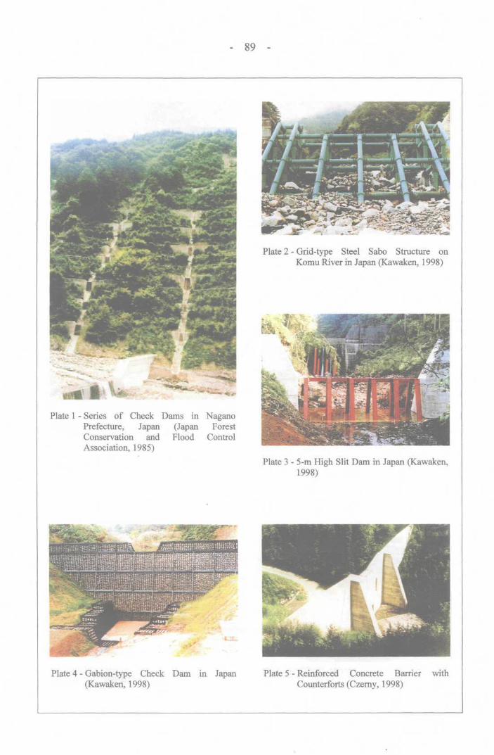
- 89 -

•it*' I

Plate 1 - Series of Check Dams in NaganoPrefecture, Japan (Japan ForestConservation and Flood ControlAssociation, 1985)

•jpV ' ̂ P».' M&3£MCMf ' ^^5» ' vflHHl

Sfe

Plate 2 - Grid-type Steel Sabo Structure onKomu River in Japan (Kawaken, 1998)

Plate 3 - 5-m High Slit Dam in Japan (Kawaken,1998)

Plate 4 - Gabion-type Check Dam in Japan(Kawaken, 1998)

Plate 5 - Reinforced Concrete Barrier withCounterforts (Czerny, 1998)

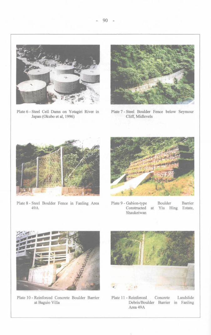
90 -

Plate 6 - Steel Cell Dams on Yotagiri River inJapan (Okubo et al, 1996)

Plate 1 - Steel Boulder Fence below SeymourCliff, Midlevels

Plate 8 - Steel Boulder Fence in Fanling Area49A

*-..» - - ' 4v-; -Plate 9 - Gabion-type Boulder Barrier

Constructed at Yiu King Estate,Shaukeiwan

Plate 10-Reinforced Concrete Boulder Barrierat Baguio Villa

Plate 11 - Reinforced Concrete LandslideDebris/Boulder Barrier in FanlingArea 49A

- 91

Plate 12 - 5-m High Reinforced Concrete Barrierat Kowloon Medical RehabilitationCentre

Plate 13-Debris Containment Berm in TuenMun Area 19

Plate 14 - 6-m High Check Dam underConstruction in Sham Tseng

Plate 15 - Use of Rubber Tires to Soften Impact on Barrier (Kawaken, 1998)

GEOTECHNICAL ENGINEERING OFFICE PUBLICATIONS

Geotechnical Manual for Slopes, 2nd Edition (1984), 300 p.(English Version), (Reprinted, 2000).

Highway Slope Manual (2000), 114 p.

Guide to Retaining Wall Design, 2nd Edition (1993), 258 p. Geoguide 1(Reprinted, 2000).

Guide to Site Investigation (1987), 359 p. (Reprinted, 1996). Geoguide 2

Guide to Rock and Soil Descriptions (1988), 186 p. (Reprinted, Geoguide 31997).

Guide to Cavern Engineering (1992), 148 p. (Reprinted, 1998). Geoguide 4

Guide to Slope Maintenance, 2nd Edition (1998), 91 p. Geoguide 5(English Version), (Reprinted, 1999).

Layman's Guide to Slope Maintenance, 2nd Edition (1998),56 p. (Bilingual), (Reprinted, 2000).

' HHJg(1998) • 56H(4^i» ' (-

Model Specification for Prestressed Ground Anchors, 2nd GeospeclEdition (1989), 164 p. (Reprinted, 1997).

Model Specification for Reinforced Fill Structures (1989), Geospec2135 p. (Reprinted, 1997).

Mid-levels Study : Report on Geology, Hydrology and SoilProperties (1982), 265 p. plus 54 drgs. (Reprinted, 1997).

HK$70(US$14.5)

HK$90(US$20)

HK$50(US$12)

HK$68(US$14)

HK$83(US$17.5)

HK$58(US$12.6)

HK$60(US$13)

HK$50(US$9.5)

HK$50(US$9.5)

Free

HK$62(US$11)

HK$58(US$10.5)

HK$534(US$86)

Prediction of Soil Suction for Slopes in Hong Kong, by M.G. GCO Publication HK$132Anderson (1984), 242 p. (Reprinted, 1996). No. 1/84 (US$24)

(Superseded by GCO Publication No. 1/85) GCO PublicationNo. 2/84

(Superseded by Geospec 1) GCO PublicationNo. 3/84

Review of Superficial Deposits and Weathering in Hong Kong, GCO Publication HK$40by J.D. Bennett (1984), 58 p. (Reprinted, 1993). No. 4/84 (US$8)

Review of Hong Kong Stratigraphy, by J.D. Bennett (1984), GCO Publication HK$2586 p. No. 5/84 (US$5.5)

Review of Tectonic History, Structure and Metamorphism of GCO Publication HK$20Hong Kong, by J.D. Bennett (1984), 63 p. No. 6/84 (US$5)

(Superseded by GCO Publication No. 1/88) GCO PublicationNo. 1/85

Groundwater Lowering by Horizontal Drains, by D.J. Craig & GCO Publication HK$74I. Gray (1985), 123 p. (Reprinted, 1990). No. 2/85 (US$12)

(Superseded by GEO Report No. 9) GCO PublicationNo. 1/88

Review of Design Methods for Excavations (1990), 187 p. GCO Publication HK$62(Reprinted, 2000). No. 1/90 (US$13.5)

Foundation Properties of Marble and Other Rocks in the Yuen GCO Publication HK$58Long - Tuen Mun Area (1990), 117 p. No. 2/90 (US$10)

Review of Earthquake Data for the Hong Kong Region (1991), GCO Publication HK$42115 p. No. 1/91 (US$11.5)

Review of Granular and Geotextile Filters (1993), 141 p. GEO Publication HK$32No. 1/93 (US$19)

Pile Design and Construction (1996), 348 p. (Reprinted, 1997). GEO Publication HK$62No. 1/96 (US$13.5)

Technical Guidelines on Landscape Treatment and GEO Publication HK$114Bio-engineering for Man-made Slopes and Retaining Walls, No. 1/2000 (US$20)by Urbis Limited (2000), 146 p.

Report on the Fei Tsui Road Landslide of 13 August 1995, - Free2 Volumes, 156 p. (Bilingual).

Report on the Shum Wan Road Landslide of 13 August 1995,2 Volumes, 123 p. (Bilingual).

Freesat

What to Do When You Receive a Dangerous Hillside Order(1996), 32 p. (Bilingual), (Reprinted, 1999).

Free

(Hong Kong) Rainfall and Landslides in 1984, by J. Premchitt GEO Report HK$118(1991), 91 p. plus 1 drg. (Reprinted, 1995). No. 1 (US$17.5)

(Hong Kong) Rainfall and Landslides in 1985, by J. Premchitt GEO Report HK$126(1991), 108 p. plus 1 drg. (Reprinted, 1995). No. 2 (US$20)

(Hong Kong) Rainfall and Landslides in 1986, by J. Premchitt GEO Report HK$126(1991), 113 p. plus 1 drg. (Reprinted, 1995). No. 3 (US$20)

Hong Kong Rainfall and Landslides in 1987, by J. Premchitt GEO Report HK$122(1991), 101 p. plus 1 drg. (Reprinted, 1995). No. 4 (US$19.5)

Hong Kong Rainfall and Landslides in 1988, by J. Premchitt GEO Report HK$106(1991), 64 p. plus 1 drg. (Reprinted, 1995). No. 5 (US$16)

Hong Kong Rainfall and Landslides in 1989, by K.L. Siu GEO Report HK$126(1991), 114 p. plus 1 drg. (Reprinted, 1995). No. 6 (US$20)

Aggregate Properties of Some Hong Kong Rocks, by T.Y. GEO Report HK$120Man, A. Cipullo, A.D. Burnett & J.M. Nash (1992), 212 p. No. 7 (US$19.5)(Reprinted, 1995).

Foundation Design of Caissons on Granitic and Volcanic GEO Report HK$62Rocks, by T.Y. Man & G.E. Powell (1991), 85 p. (Reprinted, No. 8 (US$10.5)1995).

Bibliography on the Geology and Geotechnical Engineering of GEO ReportHong Kong to December 1991, by E.W. Brand (1992), 186 p. No. 9(Superseded by GEO Report No.39)

Bibliography on Settlements Caused by Tunnelling, by E.W. GEO Report HK$48Brand (1992), 50 p. (Reprinted, 1995). (Superseded by GEO No. 10 (US$8.5)Report No.51)

Direct Shear Testing of a Hong Kong Soil under Various GEO Report HK$136Applied Matric Suctions, by J.K. Gan & D.G. Fredlund (1992), No. 11 (US$21.5)241 p. (Reprinted, 1995).

Rainstorm Runoff on Slopes, by J. Premchitt, T.S.K. Lam, J.M. GEO Report HK$121Shen and H.F. Lam (1992), 211 p. (Reprinted, 1995). No. 12 (US$19.5)

Mineralogical Assessment of Creep-type Instability at Two GEO Report HK$87Landslip Sites, by T.Y. frfan (1992), 136 p. (Reprinted, 1995). No. 13 (US$15)

Hong Kong Rainfall and Landslides in 1990, by K.Y. Tang GEO Report HK$112(1992), 78 p. plus 1 drg. (Reprinted, 1995). No. 14 (US$17)

Assessment of Stability of Slopes Subjected to Blasting GEO Report HK$56Vibration, by H.N. Wong & P.L.R. Pang (1992), 112 p. No. 15 (US$10.5)(Reprinted, 2000).

Earthquake Resistance of Buildings and Marine Reclamation GEO Report HK$48Fills in Hong Kong, by W.K. Pun (1992), 48 p. (Reprinted, No. 16 (US$8.5)1995).

Review of Dredging Practice in the Netherlands, by S.T. GEO Report HK$76Gilbert & P.W.T. To (1992), 112 p. (Reprinted, 1995). No. 17 (US$12)

Backfilled Mud Anchor Trials Feasibility Study, by C.K. Wong GEO Report HK$50& C.B.B. Thorley (1992), 55 p. (Reprinted, 1995). No. 18 (US$9)

A Review of the Phenomenon of Stress Rupture in HDPE GEO Report HK$56Geogrids, by G.D. Small & J.H. Greenwood (1993), 68 p. No. 19 (US$9.5)(Reprinted, 1995).

Hong Kong Rainfall and Landslides in 1991, by N.C. Evans GEO Report HK$111(1992), 76 p. plus 1 drg. (Reprinted, 1995). No. 20 (US$16.5)

Horizontal Subgrade Reaction for Cantilevered Retaining Wall GEO Report HK$50Analysis, by W.K. Pun & P.L.R. Pang (1993), 41 p. (Reprinted, No. 21 (US$9.5)1998).

Report on the Rainstorm of 8 May 1992, by N.C. Evans (1993), GEO Report HK$126109 p. plus 2 drgs. (Reprinted, 1995). No. 22 (US$20)

Effect of the Coarse Fractions on the Shear Strength of GEO Report HK$126Colluvium, by T.Y. Man & K.Y. Tang (1993), 223 p. No. 23 (US$20)(Reprinted, 1995).

The Use of PFA in Reclamation, by J. Premchitt & N.C. Evans GEO Report HK$52(1993), 59 p. (Reprinted, 1995). No. 24 (US$9)

Report on the Rainstorm of May 1982, by M.C Tang (1993), GEO Report HK$135129 p. plus 1 drg. (Reprinted, 1995). No. 25 (US$21)

Report on the Rainstorm of August 1982, by R.R. Hudson GEO Report HK$118(1993), 93 p. plus 1 drg. (Reprinted, 1995). NO. 26 (US$17.5)

Landslips Caused by the June 1983 Rainstorm, by E.B. Choot GEO Report HK$83(1993), 124 p. (Reprinted, 1995). No.27 (US$13)

Factors Affecting Sinkhole Formation, by Y.C. Chan (1994), GEO Report HK$4037 p. (Reprinted, 1995). No. 28 (US$7.5)

Classification and Zoning of Marble Sites, by Y.C. Chan GEO Report HK$40(1994), 37 p. (Reprinted, 1995). No. 29 (US$7.5)

Hong Kong Seawall Design Study, by P.M. Aas & A. Engen GEO Report HK$68(1993), 94 p. (Reprinted, 2000). No. 30 (US$11)

Study of Old Masonry Retaining Walls in Hong Kong, by Y.C. GEO Report HK$ 130Chan (1996), 225 p. (Reprinted, 2000). No. 31 (US$21)

Karst Morphology for Foundation Design, by Y.C. Chan & GEO Report HK$118W.K. Pun (1994), 90 p. plus 1 drg. (Reprinted, 1995). No. 32 (US$17.5)

An Evaluation of the Suitability of Decomposed Granite as GEO Report HK$38Foundation Backfill for Gravity Seawalls in Hong Kong, by No. 33 (US$7)E.B. Choot (1993), 34 p. (Reprinted, 1995).

A Partial Factor Method for Reinforced Fill Slope Design, by GEO Report HK$50H.N. Wong (1993), 55 p. (Reprinted, 2000). No. 34 (US$9)

Hong Kong Rainfall and Landslides in 1992, by P.K.H. Chen GEO Report HK$167(1993), 201 p. plus 2 drgs. (Reprinted, 1995). No. 35 (US$25.5)

Methods of Test for Soils in Hong Kong for Civil Engineering GEO Report HK$22Purposes (Phase I Tests), 1996 Edition, by P.Y.M. Chen, 90 p. No. 36 (US$5.5)

Creep, Stress Rupture and Hydrolysis of Polyester Reinforced GEO Report HK$38Geogrids, by J.H, Greenwood (1995), 67 p. No. 37 (US$7.5)

Skin Friction on Piles at the New Public Works Central GEO Report HK$97Laboratory, by J. Premchitt, I. Gray & K.K.S. Ho (1994), 158 p. No. 38 (US$16.5)(Reprinted, 1995).

Bibliography on the Geology and Geotechnical Engineering of GEO Report HK$118Hong Kong to May 1994, by E.W. Brand (1994), 202 p, No. 39 (US$19)(Reprinted, 1995). (Superseded by GEO Report No.50)

Hydraulic Fill Performance in Hong Kong, by C.K. Shen & GEO Report HK$90K.M. Lee (1995), 199 p. No. 40 (US$16)

Mineralogy and Fabric Characterization and Classification of GEO Report HK$70Weathered Granitic Rocks in Hong Kong, by T.Y. Man (1996), No. 41 (US$13.5)158 p.

Performance of Horizontal Drains in Hong Kong, by R.P. GEO Report HK$65Martin, K.L. Siu & J. Premchitt (1995), 109 p. No. 42 (US$ 17.2)

Hong Kong Rainfall and Landslides in 1993, by W.L. Chan GEO Report HK$110(1995), 214 p. plus 1 drg. No. 43 (US$18.5)

General Report on Landslips on 5 November 1993 at GEO Report HK$64Man-made Features in Lantau, by H.N. Wong & K.K.S. Ho No. 44 (US$17)(1995), 78 p. plus 1 drg.

Gravity Retaining Walls Subject to Seismic Loading, by Y.S. GEO Report HK$40Au-Yeung&K.K.S.Ho(1995),63p. No. 45 (US$8)

Direct Shear and Triaxial Testing of a Hong Kong Soil under GEO Report HK$65Saturated and Unsaturated Conditions, by J.K.M. Gan & D.G. No. 46 (US$ 12.5)Fredlund(1996),217p.

Stability of Submarine Slopes, by N.C. Evans (1995), 51 p. GEO Report HK$46No. 47 (US$8.5)

Strength Development of High PFA Content Concrete, by GEO Report HK$60W.C.Leung&WJLTse(1995),84p. No. 48 (US$10.5)

AAR Potential of Volcanic Rocks from Anderson Road GEO Report HK$58Quarries, by W.C. Leung, W.L. Tse, C.S. Mok & S.T.Gilbert No. 49 (US$10)(1995), 78 p.

Bibliography on the Geology and Geotechnical Engineering of GEO Report HK$45Hong Kong to March 1996, by E.W. Brand (1996), 111 p. No. 50 (US$9)

Bibliography on Settlements Caused by Tunnelling to March GEO Report HK$311996, by E.W. Brand (1996), 70 p. No. 51 (US$6.5)

Investigation of Some Major Slope Failures between 1992 and GEO Report HK$441995, by Y.C. Chan, W.K. Pun, H.N. Wong, A.C.O. Li &K.C. No. 52 (US$8.5)Yeo(1996),97p.

Environmental Aspects of Using Fresh PFA as Fill in GEO Report HK$30Reclamation, by K.S. Ho & P.Y.M. Chen (1996), 46 p. No. 53 (US$5.5)

Hong Kong Rainfall and Landslides in 1994, by W.L. Chan GEO Report HK$70(1996), 161 p. plus 1 drg. No. 54 (US$13.5)

Conventional and CRS Rowe Cell Consolidation Test on SomeHong Kong Clays, by J. Premchitt, K.S. Ho & N.C. Evans(1996), 93 p.

Application of Prescriptive Measures to Slopes and RetainingWalls, 2nd Edition (1999), by H.N. Wong, L.S. Pang, A.C.W.Wong, W.K. Pun & Y.F. Yu, 73 p. (Reprinted, 2000).

Study of Rainfall Induced Landslides on Natural Slopes in theVicinity of Tung Chung New Town, Lantau Island, byC.A.M. Franks (1998), 102 p. plus 3 drgs. (Reprinted, 1999).

Appraisal of Performance of Recompacted Loose Fill Slopes,by K.T. Law, C.F. Lee, M.T. Luan, H. Chen & X. Ma (1999),86 p.

Hong Kong Rainfall and Landslides in 1995, by C.K.L. Wong(1997), 125 p. plus 1 drg.

Assessment of Geological Features Related to RecentLandslides in Volcanic Rocks of Hong Kong Phase 2A - ChaiWan Study Area, by S.D.G. Campbell & N.P. Koor (1998),78 p. plus 6 drgs.

Factual Report on the November 1993 Natural TerrainLandslides in Three Study Areas on Lantau Island, by H.N.Wong, Y.M. Chen & K.C. Lam (1997), 42 p.

Area! Extent of Intense Rainfall in Hong Kong 1979 to 1995,by A.W. Malone (1997), 85 p.

A Review of Some Drained Reclamation Works in HongKong, by J.S.M. Kwong (1997), 53 p.

A Study of Hydraulic Fill Performance in Hong Kong -Phase 2, by C.K. Shen, K.M. Lee & X.S. Li (1997), 265 p.

Seismic Hazard Analysis of the Hong Kong Region, by C.F.Lee, Y.Z. Ding, R.H. Huang, Y.B. Yu, G.A. Guo, P.L. Chen& X.H. Huang (1998), 145 p. (Bilingual), (Reprinted, 2000).

> *»£• - rmm * it sis *#m$L - »

GEO ReportNo. 55

GEO ReportNo. 56

GEO ReportNo. 57

GEO ReportNo. 58

GEO ReportNo. 59

GEO ReportNo. 60

GEO ReportNo. 61

GEO ReportNo. 62

GEO ReportNo. 63

GEO ReportNo. 64

GEO ReportNo. 65

HK$35(US$7)

HK$34(US$7.5)

HK$264(US$39.5)

HK$34(US$7.5)

HK$70(US$14.5)

HK$296(US$43.5)

HK$92(US$13.5)

HK$43(US$8.5)

HK$36(US$6.5)

HK$150(US$25)

HK$80(US$15.5)

Mineralogical and Fabric Characterization and Classification ofWeathered Volcanic Rocks in Hong Kong, by T.Y. Man (1998),113 p.

GEO ReportNo. 66

HK$106(US$17)

Assessment of Geological Features Related to RecentLandslides in Volcanic Rocks of Hong Kong Phase 2B -Aberdeen Study Area, by C.A.M. Franks, S.D.G. Campbell &W.W.L. Shum (1999), 106 p. plus 8 drgs.

The New Priority Classification Systems for Slopes andRetaining Walls, by C.K.L. Wong (1998), 1 17 p. (Reprinted,1999).

Diagnostic Report on the November 1993 Natural TerrainLandslides on Lantau Island, by H.N. Wong, K.C. Lam &K.K.S. Ho (1998), 98 p. plus 1 drg.

Hong Kong Rainfall and Landslides in 1996, by C.K.L. Wong(1998), 84 p. plus 1 drg.

Site Characterisation Study - Phases 1 and 2, by N.P. Koor(1999), 207 p.

Long-term Consolidation Tests on Clays from the Chek LapKok Formation, by D.O.K. Lo & J. Premchitt (1998), 89 p.

The Natural Terrain Landslide Study Phases I and n, by N.C.Evans, S.W. Huang & J.P. King (1999), 128 p. plus 2 drgs.

Natural Terrain Landslide Study the Natural Terrain LandslideInventory, by J.P. King (1999), 127 p.

Landslides and Boulder Falls from Natural Terrain : InterimRisk Guidelines, by ERM-Hong Kong, Ltd (1998), 183 p.(Reprinted, 1999).

Report on the Landslides at Hut No. 26 Kau Wa Keng UpperVillage of 4 June 1997, by Halcrow Asia Partnership Ltd.(1998), 100 p. (Bilingual).

GEO ReportNo. 67

GEO ReportNo. 68

GEO ReportNo. 69

GEO ReportNo. 70

GEO ReportNo. 71

GEO ReportNo. 72

GEO ReportNo. 73

GEO ReportNo. 74

GEO ReportNo. 75

GEO ReportNo. 76

HK$358(US$54.5)

HK$68(US$12)

HK$90(US$17)

HK$ 1 12(US$20)

HK$292(US$43)

HK$34(US$7.5)

HK$308(US$45)

HK$208(US$32)

HK$94(US$17.5)

HK$140(US$21.5)

Report on the Landslide at Ten Thousand Buddhas' Monastery GEO Reportof 2 July 1997, by Halcrow Asia Partnership Ltd. (1998), 96 p. No. 77(Bilingual).

~ H »

HK$140(US$21 .5)

Report on the Ching Cheung Road Landslide of 3 August GEO Report1997, by Halcrow Asia Partnership Ltd. (1998), 142 p. No. 78(Bilingual).

H B MP

HK$256(US$38.5)

Investigation of Some Selected Landslide Incidents in 1997 GEO Report HK$192(Volume 1), by Halcrow Asia Partnership Ltd. (1998), 142 p. No. 79 (US$30)

Feasibility Study for QRA of Boulder Fall Hazard in Hong GEO Report HK$58Kong, by ERM-Hong Kong, Ltd (1998), 61 p. No. 80 (US$10.5)

Slope Failures along BRIL Roads : Quantitative Risk GEO Report HK$76Assessment and Ranking, by ERM-Hong Kong, Ltd (1999), No. 81 (US$15)200 p.

Contaminated Mud Disposal at East Sha Chau : Comparative GEO Report HK$52Integrated Risk Assessment, by EVS Environment No. 82 (US$12)Consultants (1999), 138 p.

Testing of Dredged Material for Marine Disposal, by EVS GEO Report HK$36Environment Consultants ( 1 999), 74 p. No. 83 (US$8)

December 1995 Investigation of Benthic Recolonization at GEO Report HK$178the Mirs Bay Disposal Site, by Binnie Consultants Limited No. 84 (US$26)(1999), 89 p.

The Use of Acoustic Doppler Current Profilers to Measure GEOReport HK$108Suspended Sediments, by Dredging Research Ltd (1999), No. 85 (US$17)34 p.

Report of the Independent Review Panel on Fill Slopes, by GEO Report HK$30J.L. Knill, P. Lumb, S. Mackey, V.F.B. de Mello, N.R. No. 86 (US$5.5)Morgenstern & B.G. Richards (1999), 36 p.

Strategic Re-assessment of Disposal Site Selection and GEOReport HK$32Management of Contaminated Mud, by EVS Environment No. 87 (US$6)Consultants (1999), 50 p.

Investigation of Some Selected Landslide Incidents in 1997 GEOReport HK$278(Volume 2), by Halcrow Asia Partnership Ltd. (1999), 202 p. No. 88 (US$41.5)

Investigation of Some Selected Landslide Incidents in 1997 GEOReport HK$200(Volume 3), by Halcrow Asia Partnership Ltd. (1999), 145 p. No. 89 (US$31)

Investigation of Some Selected Landslide Incidents in 1997 GEO Report HK$232(Volume 4), by Halcrow Asia Partnership Ltd. (1999), 147 p. No. 90 (US$35.5)

Investigation of Some Selected Landslide Incidents in 1997(Volume 5), by Halcrow Asia Partnership Ltd. (1999), 141 p.

Investigation of Some Selected Landslide Incidents in 1997(Volume 6), by Halcrow Asia Partnership Ltd. (1999), 181 p.

Seabed Ecology Studies : Composite Report, by ERM-HongKong, Ltd (1999), 182 p.

Report on the Rock Slope Failure at Cut Slope 11NE-D/C7along Sau Mau Ping Road on 4 December 1997, by B.N.Leung, S.C. Leung & C.A.M. Franks (1999), 69 p.

The Lai Ping Road Landslide of 2 July 1997, by H.W. Sun &S.D.G. Campbell (1999), 140 p. plus 2 drgs.

Review of Fill Slope Failures in Hong Kong, by H.W. Sun(1999), 87 p.

Hong Kong Rainfall and Landslides in 1997, by T.W.K. Lam(1999), 271 p. plus 2 drgs.

Preliminary Quantitative Risk Assessment of Earthquake-induced Landslides at Man-made Slopes in Hong Kong, byH.N. Wong & K.K.S. Ho (2000), 69 p.

A Review of Downhole Geophysical Methods for GroundInvestigation, by K.C. Lau (2000), 69 p.

Methods of Assessment and Monitoring of the Effects of GasPressures on Stability of Rock Cuts due to Blasting in theNear-field, by Blastronics Pty Ltd (2000), 55 p.

Cavern Area Study of Kowloon, by K. J. Roberts & P.A. Kirk(2000), 37 p. plus 1 drg.

A Study of the Effects of Blasting Vibration on GreenConcrete, by A.K.H. Kwan & P.K.K. Lee (2000), 159 p.

Report on the Kwun Lung Lau Landslide of 23 July 1994, byN.R. Morgenstern & Geotechnical Engineering Office(2000), 365 p. (English Version).

- A AH^-fc M -+= B mm

GEO ReportNo. 91

GEO ReportNo. 92

GEO ReportNo. 93

GEO ReportNo. 94

GEO ReportNo. 95

GEO ReportNo. 96

GEO ReportNo. 97

GEO ReportNo. 98

GEO ReportNo. 99

GEO ReportNo. 100

GEO ReportNo. 101

GEO ReportNo. 102

GEO ReportNo. 103

ifc&Dl

HK$208(US$32)

HK$218(US$33.5)

HK$220(US$34)

HK$88(US$14.5)

HK$264(US$39.5)

HK$58(US$10.5)

HK$338(US$49)

HK$42(US$8.5)

HK$40(US$8.5)

HK$90(US$15)

HK$70(US$12)

HK$64(US$13.5)

HK$172(US$30.5)

HK$172(US$30.5)

mum

Review of Natural Terrain Landslide Debris-resisting Barrier GEO ReportDesign, by D.O.K. Lo (2000), 91 p. No. 104

Hong Kong Rainfall and Landslides in 1998, by T.W.K. Lam GEO Report(2000), 96 p. No. 105

Suspended Sediment in Hong Kong Waters, by S. Parry GEO Report(2000), 68 p. No. 106

Review of 1997 and 1998 Landslides, by H.N. Wong & GEO ReportK.K.S. Ho (2000), 53 p. No. 107

Geotechnical Area Studies Programme - Hong Kong and GASP IKowloon (1987), 170 p. plus 4 maps. (Sold out)

Geotechnical Area Studies Programme - Central New GASP1ITerritories (1987), 165 p. plus 4 maps.

Geotechnical Area Studies Programme - West New Territories GASP IH(1987), 155 p. plus 4 maps.

Geotechnical Area Studies Programme - North West New GASP IVTerritories (1987), 120 p. plus 3 maps.

Geotechnical Area Studies Programme - North New Territories GASP V(1988), 134 p. plus 3 maps.

Geotechnical Area Studies Programme - North Lantau (1988), GASP VI124 p. plus 3 maps.

Geotechnical Area Studies Programme - Clear Water Bay GASPVH(1988), 144 p. plus 4 maps.

Geotechnical Area Studies Programme - North East New GASP VIETerritories (1988), 144 p. plus 4 maps.

Geotechnical Area Studies Programme - East New Territories GASP IX(1988), 141 p. plus 4 maps.

Geotechnical Area Studies Programme - Islands (1988), 142 p. GASP Xplus 4 maps.

Geotechnical Area Studies Programme - South Lantau (1988), GASP XI148 p. plus 4 maps.

Geotechnical Area Studies Programme - Territory of Hong GASP XHKong (1989), 346 p. plus 14 maps.

HK$58(US$11)

HK$134(US$21)

HK$152(US$23)

HK$34(US$6)

HK$240(US$40)

HK$150(US$25)

HK$150(US$25)

HK$150(US$25)

HK$150(US$25)

HK$150(US$25)

HK$150(US$25)

HK$150(US$25)

HK$150(US$25)

HK$150(US$25)

HK$150(US$25)

HK$150(US$25)

Geology of Sha Tin, by R. Addison (1986), 85 p.

Geology of Hong Kong Island and Kowloon, by P.J. Strange &R. Shaw (1986), 134 p.

Geology of the Western New Territories, by R.L. Langford,K.W. Lai, R.S. Arthurton & R. Shaw (1989), 140 p.

Geology of Sai Kung and Clear Water Bay by P.J. Strange, R.Shaw & R. Addison (1990), 111 p.

Geology of the North Eastern New Territories, K.W. Lai,S.D.G. Campbell & R. Shaw (1996), 144 p.

Geology of Lantau District by R.L. Langford, J.W.C. James, R.Shaw, S.D.G. Campbell, P.A. Kirk & RJ. Sewell (1995),173 p.

Geology of Yuen Long by D.V. Frost (1992), 69 p.

GeologicalMemoir No. 1

GeologicalMemoir No. 2

GeologicalMemoir No. 3

GeologicalMemoir No. 4

GeologicalMemoir No. 5

GeologicalMemoir No. 6

Sheet ReportNo. 1

HK$50(US$9)

HK$78(US$12.5)

HK$97(US$17)

HK$87(US$13)

HK$98(US$17.5)

HK$136(US$28.2)

Free

Geology of Chek Lap Kok by R.L. Langford (1994), 61 p. Sheet ReportNo. 2

Free

Geology of Tsing Yi by R.J. Sewell & J.A. Fyfe (1995), 43 p. Sheet ReportNo. 3

Free

Geology of North Lantau Island and Ma Wan by R. J. Sewell Sheet Report& J.W.C. James (1995), 46 p. No. 4

Geology of Ma On Shan by RJ. Sewell (1996), 45 p.

Geological Landscapes of Hong Kong (1998), 61 p. (Bilingual).' 613

Sheet ReportNo. 5

Geochemical Atlas of Hong Kong (1999), 110 p.

The Quaternary Geology of Hong Kong, by J.A. Fyfe, R. Shaw,S.D.G. Campbell, K.W. Lai & P.A. Kirk (2000), 210 p. plus6 maps. (In press).

The Pre-Quaternary Geology of Hong Kong, by RJ. Sewell,S.D.G. Campbell, CJ.N. Fletcher, K.W. Lai & P.A. Kirk(2000), 181 p. plus 4 maps. (In press).

Free

Free

HK$130

HK$200(US$34)

HK$220(US$37)

HK$220(US$37)

San Tin : Solid and Superficial Geology (1:20000 map) MapHGM20, HK$80(1989), 1 map. Sheet!

Sheung Shui: Solid and Superficial Geology (1:20 000 map) Map HGM 20, HK$80(1991),! map. Sheets

Kat O Chau : Solid and Superficial Geology (1:20 000 map) Map HGM 20, HK$80(1992), 1 map. Sheet 4

Tsing Shan (Castle Peak) : Solid and Superficial Geology Map HGM 20, HK$80(1:20 000 map) (1988), 1 map. Sheet 5

Yuen Long : Solid and Superficial Geology (1:20 000 map) Map HGM 20, HK$80(1988), 1 map. Sheet 6

Sha Tin : Solid and Superficial Geology (1:20000 map) Map HGM 20, HK$80(1986), 1 map. Sheet?

Sai Kung Peninsula: Solid and Superficial Geology (1:20 000 Map HGM 20, HK$80map) (1989), 1 map. Sheet 8

Tung Chung : Solid and Superficial Geology (1:20 000 map) Map HGM 20, HK$80(1994), 1 map. Sheet 9

Silver Mine Bay : Solid and Superficial Geology (1:20000 Map HGM 20, HK$80map) (1991), 1 map. Sheet 10

Hong Kong and Kowloon : Solid and Superficial Geology Map HGM 20, HK$80(1:20 000 map) (1986), 1 map. Sheet 11

Clear Water Bay : Solid and Superficial Geology (1:20000 Map HGM 20, HK$80map) (1989), 1 map. Sheet 12

Shek Pik : Solid and Superficial Geology (1:20000 map) Map HGM 20, HK$80(1995), 1 map. Sheet 13

Cheung Chau : Solid and Superficial Geology (1:20 000 map) Map HGM 20, HK$80(1995), 1 map. Sheet 14

Hong Kong South and Lamma Island : Solid and Superficial Map HGM 20, HK$80Geology (1:20 000 map) (1987), 1 map. Sheet 15

Waglan Island: Solid and Superficial Geology (1:20 000 map) Map HGM 20, HK$80(1989), 1 map. Sheet 16

San Tin: Solid Geology (1:20 000 map) (1994), 1 map. Map HGM20S, HK$80Sheet 2

Lo Wu : Superficial Geology (1:5 000 map) (1990), 1 map. Map HOP 5A, HK$100Sheet 2-NE-D

Lo Wu : Solid Geology (1:5 000 map) (1990), 1 map. Map HOP 5B, HK$100Sheet 2-NE-D

Deep Bay: Superficial Geology (1:5 000 map) (1989), 1 map. Map HOP 5A, HK$100Sheet 2-SW-C

Deep Bay: Solid Geology (1:5 000 map) (1989), 1 map. Map HOP 5B, HK$100Sheet 2-SW-C

Shan Pui: Superficial Geology (1:5 000 map) (1989), 1 map. Map HOP 5A, HK$100Sheet 2-SW-D

Shan Pui: Solid Geology (1:5 000 map) (1989), 1 map. Map HOP 5B, HK$100Sheet 2-SW-D

Mai Po: Superficial Geology (1:5 000 map) (1990), 1 map. Map HGP 5A, HK$100Sheet 2-SE-A

Mai Po: Solid Geology (1:5 000 map) (1990), 1 map. Map HGP 5B, HK$100Sheet 2-SE-A

Lok Ma Chau : Superficial Geology (1:5 000 map) (1990), Map HGP 5A, HK$1001 map. Sheet 2-SE-B

Lok Ma Chau: Solid Geology (1:5 000 map) (1990), 1 map. Map HGP 5B, HK$100Sheet 2-SE-B

Man Kam To : Superficial Geology (1:5000 map) (1990), Map HGP 5A, HK$100Imap. Sheet 3-NW-C

Man Kara To: Solid Geology (1:5 000 map) (1990), 1 map. Map HGP 5B, HK$100Sheet3-NW-C

Tin Shui Wai : Superficial Geology (1:5 000 map) (1989), Map HGP 5A, HK$1001 map. Sheet 6-NW-A

Tin Shui Wai: Solid Geology (1:5 000 map) (1989), 1 map. Map HGP 5B, HK$100Sheet6-NW-A

YuenLong: Superficial Geology (1:5 OOOmap) (1989), Imap. MapHGPSA, HK$100Sheet6-NW-B

Yuen Long: Solid Geology (1:5 000 map) (1989), 1 map. Map HGP 5B, HK$100Sheet 6-NW-B

Hung Shui Kiu : Superficial Geology (1:5 000 map) (1989), Map HOP 5A, HK$100Imap. Sheet 6-NW-C

Hung Shui Kiu: Solid Geology (1:5 000 map) (1989), 1 map. Map HOP 5B, HK$100Sheet 6-NW-C

Muk Kiu Tau : Superficial Geology (1:5 000 map) (1990), Map HGP 5A, HK$1001 map. Sheet 6-NW-D

Muk Kiu Tau : Solid Geology (1:5 000 map) (1990), 1 map. Map HOP 5B, HK$100Sheet 6-NW-D

Tsuen Wan (Part): Solid & Superficial Geology (1:5 000 map) Map HGP 5, HK$ 100(1995), 1 map. Sheet 6-SE-D

Ma On Shan : Solid Geology (1:5 000 map) (1996), 1 map. Map HGP 5B, HK$100Sheet 7-NE-D,C(part)

Chek Lap Kok : Solid & Superficial Geology (1:5 000 map) Map HGP 5, HK$100(1993), 1 map. Sheet 9-NE-C/D

Tung Chung Wan: Solid & Superficial Geology (1:5 000 map) Map HGP 5, HK$100(1995), 1 map Sheet 9-SE-A

Pok To Yan : Solid & Superficial Geology (1:5000 map) Map HGP 5, HK$100(1997), 1 map. Sheet 9-SE-B

Lantau Peak : Solid & Superficial Geology (1:5000 map) Map HGP 5, HK$100(1996), 1 map. Sheet 9-SE-C

Sunset Peak : Solid & Superficial Geology (1:5000 map) Map HGP 5, HK$100(1996), Imap. Sheet9-SE-D

Yam O Wan : Solid & Superficial Geology (1:5000 map) Map HGP 5, HK$100(1995), 1 map. Sheet 10-NW-B

Siu Ho : Solid & Superficial Geology (1:5 000 map) (1994), Map HGP 5, HK$1001 map. Sheet 10-NW-C

Chok Ko Wan (Penny's Bay) : Solid & Superficial Geology Map HGP 5, HK$100(1:5 000 map) (1994), Imap. Sheet 10-NW-D

Ma Wan: Solid and Superficial Geology (1:5 000map) (1994), Map HGP 5, HK$100lmap. Sheet 10-NE-A

Tsing Yi: Solid & Superfical Geology (1:5 000 map) (1995), Map HOP 5, HK$1001 map. Sheet 10-NE-B/D

Pa Tau Kwu : Solid and Superficial Geology (1:5 000 map) Map HOP 5, HK$100(1994), 1 map. Sheet 10-NE-C

Tai Ho : Solid and Superficial Geology (1:5 000 map) (1995), Map HGP 5, HK$1001 map. Sheet 10-SW-A

ORDERING INFORMATION IS GIVEN ON THE NEXT PAGE

Copies of GEO publications (except Sheet Reports, 1:5 000 maps and other reports which are free of charge) may be ordered Inwriting to: J

Publications Sales Section,Information Services Department,Room 402, 4th Floor, Murray Building, @Clff 9FHKGarden Road, Central, f^mUMHong Kong, ^K (852) 3593 7482Fax (852) 2598 7482

The Information Services Department will issue an invoice upon receipt of a written order> •

In Hong Kong, publications may be directly purchased from:

Government Publications Centre,Ground Floor, Low Block,Queensway Government Offices, &JfFPWa%&&66Queensway, flpj (852) 2523 7195Hong Kong.Fax (852) 2523 7195

Requests for copies of Geological Survey Sheet Reports and other reports which are free of charge should be directed to:

Chief Geotechnical Engineer/Special Projects,Geotechnical Engineering Office, ±7fcXCivil Engineering Department,Civil Engineering Building,101 Princess Margaret Road,Homantin,Kowloon, f(X (852) 2714 0275Hong Kong.Fax (852) 2714 0275

1 :5 000 maps may be purchased from:1:5

Map Publications Centre/HK,Survey & Mapping Office,Lands Department,23th Floor, MX (852) 2521 8726North Point Government Offices,333 Java Road, North Point,Hong Kong,Fax (852) 2521 8726

All prices given in this List are for information only and may be changed without notice. TTie US$ prices shown are for overseasorders and are inclusive of surface postage to anywhere in the world. An additional bank charge of HK$50 or USW.50 is requiredper cheque made in currencies other than Hong Kong dollars. Cheques, bank drafts or money orders must be made payable toTHE GO\nERNMENT OF TIffi

Latest information on the list of GEO publications can be found at the website http*7/www.info.gov.hk/ced on the InternetAbstracts for these documents can also be found at the same website.

" S

This book is due for return or renewal on the date shownunless previously recalled. Fines may be incurred for latereturn.

DATE DUE

LB 551.30/ L/9Lo, D* 0. K.Review of natural terrainlandslide debris-resistingbarrier designHong Kong : GeotechnicalEngineering Office, Civil