three methods for measuring perception - center for...
TRANSCRIPT

1. Magnitude estimation2. Matching3. Detection/discrimination
Three methods for measuring perception
Have subject rate (e.g., 1-10) some aspect of a stimulus(e.g., how bright it appears or how load it sounds)..
Magnitude estimation
P = k Sn
P: perceived magnitudeS: stimulus intensityk: constant
Relationship between intensity of stimulus and perception of magnitude follows the same general equation in all senses
Steven’s power law

In a matching experiment, the subject's task is to adjust one of two stimuli so that they look/sound the same in some respect.
Matching
Example: brightness matching
In a detection experiment, the subject's task isto detect small differences in the stimuli.
Psychophysical procedures for detection experiments:• Method of adjustment.• Yes-No/method of constant stimuli.• Simple forced choice.• Two-alternative force choice
Detection/discrimination

Ask observer to adjust the intensity of the light until they judge it to be just barely detectable
Example: you get fitted for a new eye glasses prescription. Typically the doctor drops in different lenses and asks you if this lens is better than that one.
Method of adjustment
Do these data indicate that Laurie’s threshold is lower than Chris’s threshold?
Perc
ent
“yes
” res
pons
es
Tone intensity
Yes/no method of constant stimuli
• Present signal on some trials, no signal on other trials (catch trials).
• Subject is forced to respond on every trial either ``Yes” the thing was presented'' or ``No it wasn't'’. If they're not sure then they must guess.
• Advantage: We have both types of trials so we can count both the number of hits and the number of false alarms to get an estimate of discriminability independent on the criterion.
• Versions: simple forced choice, 2AFC, 2IFC
Forced choice

Tumor present
Tumorabsent
Doctor responds“yes”
Doctor responds“no”
Hit Miss
Falsealarm
Correctreject
Simple forced choice:four possible outcomes
Tumor present
Tumorabsent
Doctor responds“yes”
Doctor responds“no”
Hit Miss
Falsealarm
Correctreject
Information acquistisition

Tumor present
Tumorabsent
Doctor responds“yes”
Doctor responds“no”
Hit Miss
Falsealarm
Correctreject
Criterion shift
Two components to the decision-making: information and criterion.
• Information: Acquiring more information is good. The effect of information is to increase the likelihood of getting either a hit or a correct rejection, while reducing the likelihood of an outcome in the two error boxes.
• Criterion: Different people may have different bias/criterion. Some may may choose to err toward "yes" decisions. Others may choose to be more conservative and say "no” more often.
Information and criterion
N S+N
Internal response
Prob
abili
ty
d’
Internal response: probability of occurrence curves
N: noise only (tumor absent)
S+N: signal plus noise (tumor present)
Discriminability (d’ or “d-prime”) is the distance between the N and S+N curves
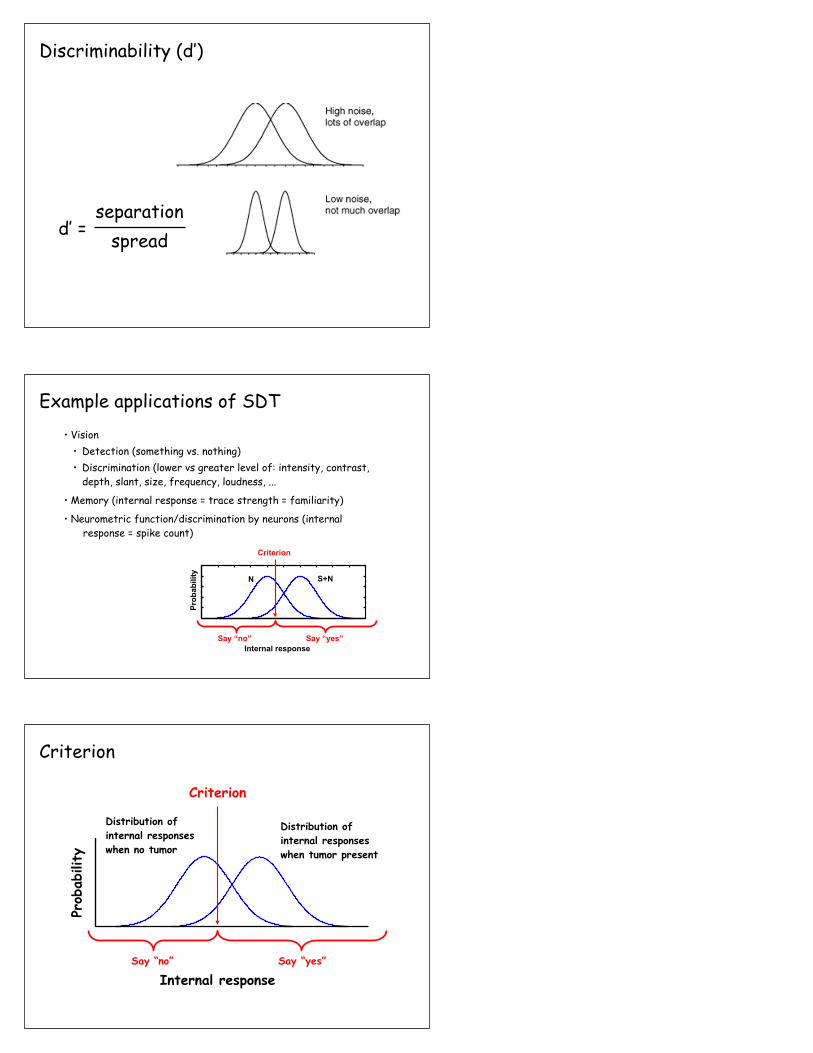
d’ = separation
spread
Discriminability (d’)
N S+N
Criterion
Internal response
Prob
abili
ty
Say “yes”Say “no”
• Vision• Detection (something vs. nothing)• Discrimination (lower vs greater level of: intensity, contrast,
depth, slant, size, frequency, loudness, ...
• Memory (internal response = trace strength = familiarity)
• Neurometric function/discrimination by neurons (internal response = spike count)
Example applications of SDT
Criterion
Internal response
Prob
ability
Criterion
Say “yes”Say “no”
Distribution of internal responses when no tumor
Distribution of internal responses when tumor present

Hits: respond “yes” when tumor present
Internal response
Prob
ability
Criterion
Say “yes”Say “no”
Distribution of internal responses when no tumor
Distribution of internal responses when tumor present
Correct rejects: respond “no” when tumor absent
Internal response
Prob
ability
Criterion
Say “yes”Say “no”
Distribution of internal responses when no tumor
Distribution of internal responses when tumor present
Misses: respond “no” when present
Internal response
Prob
ability
Criterion
Say “yes”Say “no”
Distribution of internal responses when no tumor
Distribution of internal responses when tumor present
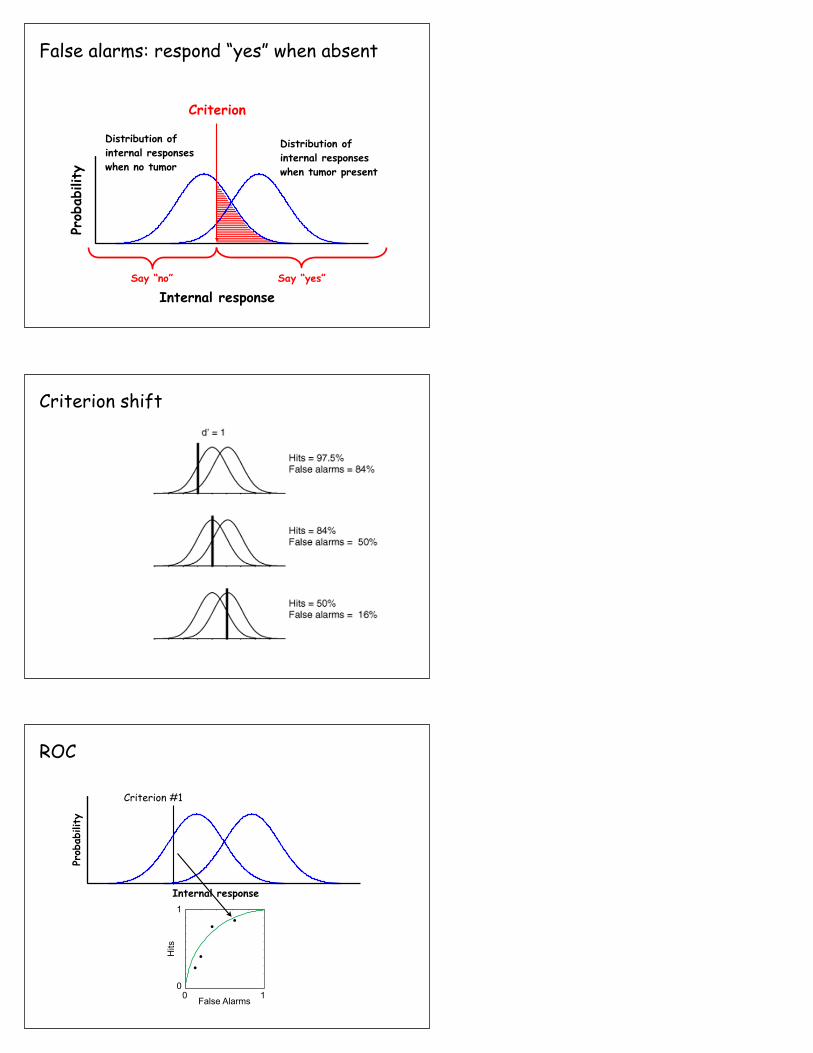
False alarms: respond “yes” when absent
Internal response
Prob
ability
Criterion
Say “yes”Say “no”
Distribution of internal responses when no tumor
Distribution of internal responses when tumor present
Criterion shift
Internal response
Prob
ability
False Alarms
Hits
0 1
1
0
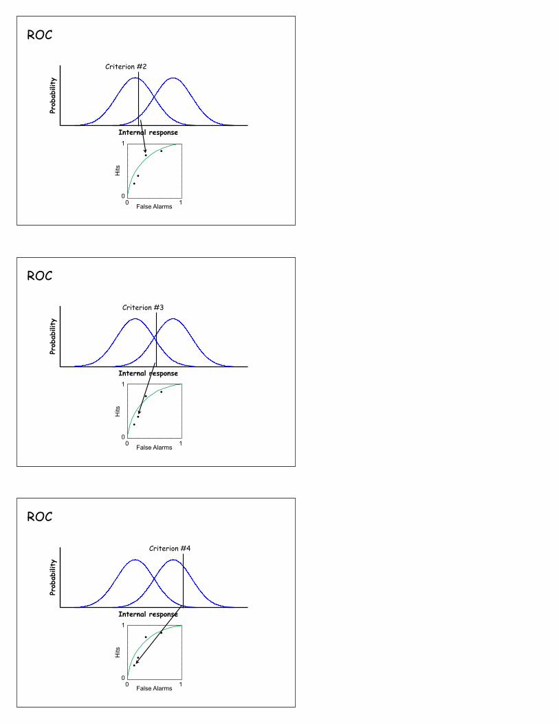
ROC
Criterion #1
Internal response
Prob
ability
False Alarms
Hits
0 1
1
0
ROC
Criterion #2
Internal response
Prob
ability
False Alarms
Hits
0 1
1
0
ROC
Criterion #3
Internal response
Prob
ability
False Alarms
Hits
0 1
1
0
ROC
Criterion #4

Receiver operating characteristic (ROC)
N S+N
z[p(FA)]
z[p(
H)]
ROC: Gaussian case
Prob
abili
ty
c
ROC: Gaussian case
N S+N
x
Prob
abili
ty
0 ʹ′dc
c = z[p(CR)] ʹ′d = z[p(H)] + z[p(CR)] = z[p(H)] − z[p(FA)]
z[p(CR)] z[p(H)]

S+N
N
c
Gaussian unequal variance
Text
Rapid estimation of full ROC:confidence ratings
Internal response
Prob
ability
“1” “2” “3” “5”“4”
False Alarms
Hits
0 1
1
0
123
4
5
• Your ability to perform a detection/discrimination task is limited by internal noise.
• Information (e.g., signal strength) and criterion (bias) are the 2 components that affect your decisions, and they each have a different kind of effect.
• Because there are 2 components (information & criterion), we need to make 2 measurements to characterize the difficulty of the task. By measuring both hits & false alarms we get a measure of discriminability (d’) that is independent of criterion.
SDT review

1
2
3
d’
Signal intensity
Low intensity High intensity
Measuring thresholds
Two-alternative forced choice
• Two options presented on each trial:
• Two stimuli presented simultaneously at two different positions (e.g., one of which has higher contrast).
• Two stimuli presented sequentially at the same position.• One stimulus presented with two possible choices (e.g., moving right
or left).
• Subject is forced to pick one of the two options. If they're not sure then they must guess.
• Feedback (correct/incorrect or $) provided after each trial.
• Advantage: Two options with feedback balances criterion so we can measure proportion correct.
Staircase

Absolute and relative thresholds
Background intensity
Dif
fere
nce
in in
tens
ity
Abs
olut
e th
resh
old
Relative thresholds
Weber’s law
Ernst Weber, c1850

Gustav Fechner, c1850
Background intensity
Inte
rnal
res
pons
eIn
crea
se in
inte
nsit
y
Weber’s law
Fechner’s analysis
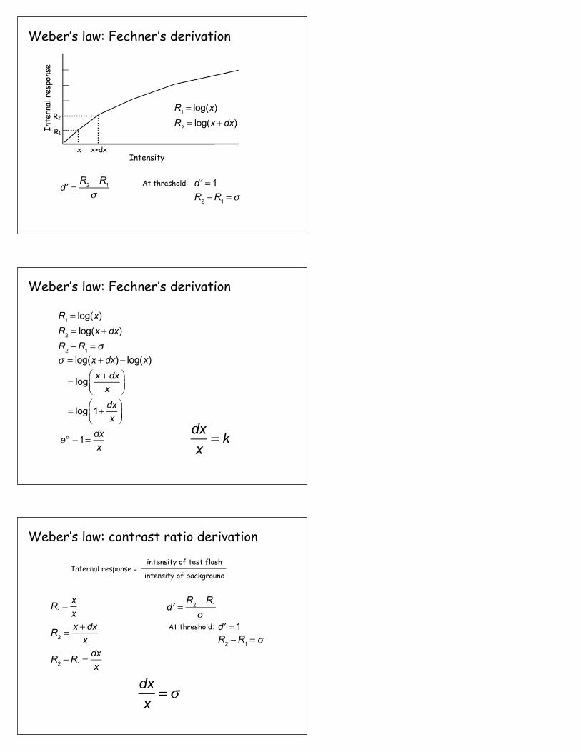
Weber’s law: Fechner’s derivation
Intensity
Inte
rnal
res
pons
e
x x+dx
R1
R2
R1 = log(x)R2 = log(x + dx)
′d =R2 −R1
σAt threshold: ′d = 1
R2 −R1 = σ
Weber’s law: Fechner’s derivation
R2 −R1 = σ
R1 = log(x)R2 = log(x + dx)
σ = log(x + dx)− log(x)
= log x + dxx
⎛⎝⎜
⎞⎠⎟
= log 1+ dxx
⎛⎝⎜
⎞⎠⎟
eσ −1= dxx
dxx
= k
Weber’s law: contrast ratio derivation
R1 =xx
Internal response =intensity of test flash
intensity of background
R2 =x + dxx
R2 −R1 =dxx
′d =R2 −R1
σAt threshold: ′d = 1
R2 −R1 = σ
dxx
= σ

Weber's law: To perceive a difference between a background level x and the background plus some stimulation x+dx the size of the difference must be proportional to the background, that is, dx = k x where k is a constant.
Fechner's interpretation: The relationship between the stimulation level x and the perceived sensation s(x) is logarithmic, s(x) = log(x).
Main difference: Fechner's is an interpretation of Weber's law, a hypothesis.
Visualstimulus
Neuronalresponse
Behavioraljudgement
Neurometric function Psychometric function
?Choice probability
Psychometric functionNeurometric function
FixationPoint
Pref target
Null target
10 deg
Receptive field
DotsAperture
Fix Pt
Dots
Targets
1 sec
Behavioral protocol
Two-alternative forced choice
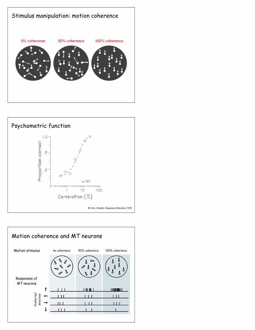
0% coherence 50% coherence 100% coherence
Stimulus manipulation: motion coherence
Britten, Shadlen, Newsome & Movshon, 1992
Psychometric function
no coherence 50% coherence 100% coherenceMotion stimulus
Responses of MT neurons
Pref
erre
d di
rect
ion
Motion coherence and MT neurons

Motion coherence and MT neurons
Each tick is anaction potential
Each line corresponds to a stimulus presentation
Average acrossall trials
Neural responses are noisy
Firi
ng r
ate
(sp/
sec)
Tria
l num
ber
Time (msec)
Perceptual decisionDecision rule: Monitor the responses of two neurons on each trial, the one being recorded and another selective for the opposite motion direction. Choose ‘pref’ if pref response > non-pref response.
fp (r) : response PDF for pref direction
fn (r) : response PDF for non-pref direction
Neuronal response
Prob
abili
ty
r
fp (r)
fn fpfn (r)
Neuronal response
Prob
abili
ty
fn fp
fn ( ʹ′r )d ʹ′r0
r
∫ = Fn (r)
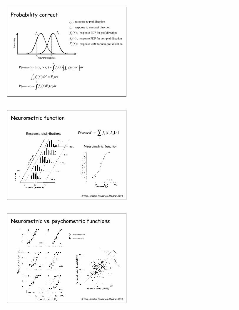
P(correct) = fp0
∞
∫ (r)Fn (r)dr
rp : response to pref direction
rn : response to non-pref direction
fp (r) : response PDF for pref direction
fn (r) : response PDF for non-pref direction
Fn (r) : response CDF for non-pref direction
P(correct) = P(rp > rn ) = fp0
∞
∫ (r) fn ( ʹ′r )d ʹ′r0
r
∫⎡⎣ ⎤⎦dr
Probability correct
rprn
Response distributions
Neurometric function
Neurometric function
Britten, Shadlen, Newsome & Movshon, 1992
P(correct) = fp[r]Fn[r]r∑
Response (spikes/trial)
0.2 0.4 0.6 0.8 7.0
P (null > crit)
6.4%
I 1 1 ““‘I ’ I ’ ,'"I
1 .o 10.0 100 Correlation (%)
Figure 5. Analysis of physiological data. A, This three-dimensional plot illustrates frequency histograms of responses obtained from a single MT neuron at five different correlation levels. The horizontal axis shows the amplitude of the neuronal response, and the vertical axis indicates the number of trials on which a particular response was obtained. The depth axis shows the correlation of motion signal used to elicit the response distributions. Open bars depict responses obtained for motion in the neuron’s preferred direction, while solid bars illustrate responses for null direction motion. For this neuron, each distribution is based on 60 trials. B, ROCs for the five pairs of preferred-null response distributions illustrated in A. Each point on an ROC depicts the proportion of trials on which the preferred direction response exceeded a criterion level plotted against the proportion of trials on which the null direction response exceeded criterion. Each ROC was generated by increasing the criterion level from 0 to 120 spikes in one-spike increments. Increased separation of the preferred and null response distributions in A leads to an increased deflection of the ROC away from the diagonal. C, A neurometric function that describes the sensitivity of an MT neuron to motion signals of increasing strength. The curve shows the performance of a simple decision model that bases judgements of motion direction on responses like those illustrated in A. The proportion of correct choices made by the model is plotted against the strength of the motion signal. The proportion of correct choices at a particular correlation level is simply the normalized area under the corresponding ROC curve in B. For this neuron, data were obtained at seven correlation levels; response distributions and ROC curves are illustrated for five of these levels in A and B. The neurometric function was fitted with sigmoidal curves of the form given in Equation 1. In this experiment, neuronal threshold (a) was 4.41 correlation and the unitless siope parameter for the neurometric function (p) was 1.30.
4752 Britten et al. l MT Neurons and Psychophysical Performance
at roughly equal rates as the criterion response increased from 1 to 100 impulses/trial. In general, the curvature of the ROC away from the diagonal indicates the separation of the preferred and null response distributions (Bamber, 1975).
Green and Swets (1966) showed formally that the normalized area under the ROC corresponds to the performance expected of an ideal observer in a two-alternative, forced-choice psycho- physical paradigm like the one employed in the present study. Again, one can intuit that this is reasonable. At 12.8% corre- lation, 99% of the area of the unit square in Figure 5B falls beneath the ROC, corresponding to the near-perfect perfor- mance we would expect based on the response distributions for 12.8% correlation in Figure 5.4. In contrast, only 51% of the unit square falls beneath the ROC for 0.8% correlation, corre- sponding as expected to random performance.
For each correlation level tested, we used this method to compute the probability that the decision rule would yield a correct response, and the results are shown in Figure 5C. These data capture the sensitivity of the neuron to directional signals in the same manner that the psychometric function captures perceptual sensitivity to directional signals. As for the psycho- metric data, we fitted the neurometric data with smooth curves of the form given by Equation 1. This function provided an excellent description of the neurometric data; the fit could be rejected for only 2 of the 2 16 neurometric functions in our data set (x2 test, p < 0.05). Application of Equation 2 resulted in a significantly improved fit for only one neuron. For the example in Figure 5C, the threshold parameter, (Y, was 4.4% correlation, and the slope parameter, & was 1.30. For each neurometric function, these parameters can be compared to the equivalent parameters obtained from the corresponding psychometric function.
1 10 100 1 10 100
Correlation (%)
Figure 6. Psychometric and neurometric functions obtained in six experiments. The open symbols and broken lines depict psychometric data, while the solid symbols and solid lines represent neurometric data. The six examples illustrate the range of relationships present in our data. A, Results of the experiment illustrated in Figures 4 and 5. Psycho- physical and neuronal data were statistically indistinguishable in this experiment. Thresholds and slope parameters are given in the captions for Figures 4 and 5. B, A second experiment in which psychometric and neurometric data were statistically indistinguishable. Psychometric 01 = 17.8% correlation, p = 1.20; neurometric o( = 23.0% correlation, (3 = 1.31. C, An experiment in which psychophysical threshold was sub- stantially lower than neuronal threshold. Psychometric 01 = 3.7% cor- relation, p = 1.68; neurometric (Y = 14.8% correlation, @ = 1.49. D, An experiment in which neuronal threshold was substantially lower than psychophysical threshold. Psychometric (Y = 13.0% correlation, (3 = 2.15; neurometric LY = 4.7% correlation, fl= 1.58. E, An experiment in which thresholds were similar but slopes were dissimilar. Psychometric LY = 3.9% correlation, B = 1.36; neurometric 01 = 4.0% correlation, p = 0.79. F, An experiment in which threshold and slope were dissimilar. Psychometric (Y = 3.1% correlation, (3 = 0.91; neurometric LY = 27.0% correlation, 0 = 1.81.
to 120 impulses/trial, the proportion of preferred direction re- sponses exceeding criterion also fell toward zero. Thus, the ROC for 12.8% correlation fell along the upper and left margins of the unit square in Figure 5B (triangles). In contrast, the ROC for 0.8% correlation fell near the diagonal line bisecting the unit square (open circles); since the preferred and null response dis- tributions were very similar at 0.8% correlation, the proportion of preferred and null direction responses exceeding criterion fell
Comparison of psychometric and neurometric functions. Fig- ure 6A shows the psychometric and neurometric functions ob- tained from the experiment illustrated in Figures 4 and 5. The two functions are remarkably similar both in their location along the abscissa and in their overall shape. The apparent similarity of the two functions was reflected in a close correspondence between the threshold parameters, o(, and the slope parameters, p, obtained from the Weibull fits (Eq. 1) to the two data sets. The neurometric threshold of 4.4% correlation compared fa- vorably to the psychometric threshold of 6.1% correlation, and the slope parameters were similar as well (neurometric p = 1.30; psychometric p = 1.17). This similarity of psychometric and neurometric data was a common feature of our data, and Figure 6B illustrates a second example. Although the absolute threshold levels were higher under the conditions of this experiment, the neurometric and psychometric data sets were again quite similar (neuronal: CY = 23.0%, p = 1.3 1; psychophysical: (Y = 17.8%, p = 1.20). Higher absolute thresholds typically occurred when the properties of the neuron under study required a psychophysi- tally nonoptimal presentation of the discriminanda (e.g., un- usually small receptive fields, large eccentricities, or high speeds). The remaining panels in Figure 6 exemplify the range of vari-
ation in our data. Neuronal and psychophysical thresholds could be strikingly dissimilar, with either the neuron (Fig. 60) or the monkey (Fig. 6CJ’) being more sensitive. The slope parameters could also appear dissimilar (Fig. 6E,F), but significant differ- ences in slope were observed less frequently than significant differences in threshold (see below).
A particularly surprising aspect of our data was the existence of MT neurons that were substantially more sensitive to motion
Neurometric vs. psychometric functions
psychometric
neurometricThe Journal of Neuroscience, December 1992, fZ(l2) 4755
A monkey J --f-
/
/
/
/
-k monkey E
/
E 1 m,onkey YT , , ,
IO 15 20
Mean neuronal threshold
L I I I
I
1.2 1.4 1.6
Mean neuronal slope
Figure 9. A comparison of average neuronal and psychophysical per- formance across animals. A, The geometric mean of neuronal threshold is plotted against the geometric mean of psychophysical threshold for each of the three animals in the study. The vertical error bars indicate SEM for neuronal threshold, while the horizontal error bars show SEM for psychophysical threshold. The broken line is the best-fitting regres- sion through the data points. B, The geometric mean of neurometric slope is plotted against the geometric mean of psychometric slope. Error bars and the regression line are as described in A.
of the variance in psychophysical cx (rz, the amount of variance accounted for, = 0.438). Adding neuronal threshold to the model as a coregressor revealed a significant predictive effect of neu- ronal threshold (p < O.Ol), but the effect was small, accounting for only an additional 2% of the variance in psychophysical threshold (r* = 0.458). Thus, experiment-to-experiment varia- tions in neuronal threshold were not highly correlated with vari-
ations in psychophysical threshold, even though the means were strikingly similar (e.g., Fig. 7).
Figure 10 amplifies this point by showing the relationship of neuronal to psychophysical threshold in richer detail. The scat- terplot depicts the actual neuronal and psychophysical thresh- olds measured in each of the 2 16 experiments in our sample. The solid circles indicate experiments in which the neurometric and psychometric functions were statistically indistinguishable as described earlier; the open circles show experiments in which the two data sets were demonstrably different. The broken di-
Neuronal threshold (%)
Figure 10. A comparison of absolute neuronal and psychophysical threshold for the 2 16 experiments in our sample. Solid circles indicate experiments in which neuronal and psychophysical threshold were sta- tistically indistinguishable; open circles illustrate experiments in which the two measures were significantly different. The broken diagonal is the line on which all points would fall if neuronal threshold predicted psychophysical threshold perfectly. The frequency histogram at the up- per right was formed by summing across the scatterplot within diago- nally oriented bins, The resulting histogram is a scaled replica of the distribution of threshold ratios depicted in Figure 7.
agonal line depicts the line of equality on which all points would fall if neuronal threshold perfectly predicted psychophysical threshold. Summing within a diagonally arranged set of bins leads to the frequency histogram in the upper right comer of Figure 10; this is simply a scaled replica of the distribution of threshold ratios shown in Figure 7. Despite the symmetrical distribution of the ratios about unity, the scatterplot reveals only a modest correlation between the two measures (r = 0.29), and most of this correlation is accounted for by the interanimal differences illustrated in Figure 9A. Thus, psychophysical and neuronal thresholds are not strongly correlated on an cell-by- cell basis, although they are closely related on the average. The absence of a strong cell-to-cell correlation is not surprising since neuronal sensitivity to motion direction varies widely (even within MT) whereas a monkey’s psychophysical sensitivity is relatively constant for any given set of stimulus conditions.
Efect of integration time on neuronal and psychophysical thresholds. The comparison of neuronal and psychophysical thresholds summarized in Figure 7 is based on experiments in which the monkey was required to view the random dot stimulus for 2 full seconds before indicating its judgement of motion direction. A potential flaw in the analysis results from the un- known time interval over which the monkey integrated infor- mation in reaching its decision. Temporal integration can in- fluence both neuronal and psychophysical thresholds, and the comparison captured in Figure 7 is reasonable only if the in- tegration interval is similar for both sets of data. For the phys- iological data presented thus far, the integration interval was always 2 set since construction of the ROCs was always based
Britten, Shadlen, Newsome & Movshon, 1992
Visualstimulus
Neuronalresponse
Behavioraljudgement
Neurometric function Psychometric function
?Choice probability
Psychometric functionNeurometric function
Shadlen, Britten, Newsome & Movshon, 1996
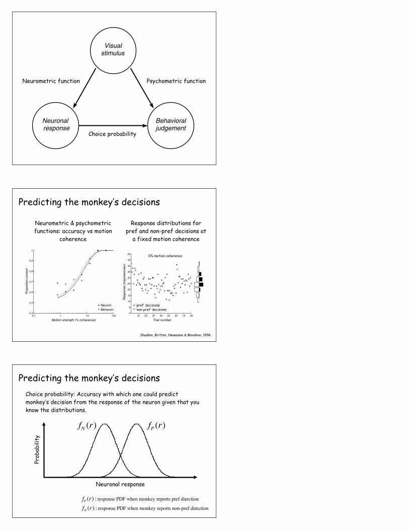
Predicting the monkey’s decisions
Neurometric & psychometric functions: accuracy vs motion
coherence
Response distributions for pref and non-pref decisions at
a fixed motion coherence
0% motion coherence
0.1 1 10 100
Motion strength (% coherence)10 20 30 40 50 60 70 80
Trial number
0
5
10
15
20
25
30
35
40
45
50
Res
pons
e (im
puls
es/s
ec)
0.4
0.5
0.6
0.7
0.8
0.9
1
Pro
port
ion
corr
ect
NeuronBehavior
Correct trialsError trials‘pref’ decisions‘non-pref’ decisions
Neuronal response
Prob
abili
ty
fP (r)fN (r)
Choice probability: Accuracy with which one could predict monkey’s decision from the response of the neuron given that you know the distributions.
Predicting the monkey’s decisions
fP (r) : response PDF when monkey reports pref direction
fN (r) : response PDF when monkey reports non-pref direction

Britten, Newsome, Shadlen, Celebrini & Movshon, 1996
Choice probability
Example neuron Across all neurons recorded
!" Decision
Pooled "up" signal
Pooled "down" signal
MT neuron pool
+
+
Pooling noise
Pooling noise
1 100.5
0.55
0.6
0.65
0.7
Cho
ice
prob
abili
ty
Threshold (% coherence)
A
B
C
D
Shadlen, Britten, Newsome & Movshon, 1996
Computational model
• Noise is partially correlated across neurons.• Responses are pooled non-optimally over large populations of
neurons including those that are not the most selective.• Additional noise is added after pooling.