traction and tractor performance - asabe technical information library

This is not a peer-reviewed article. Pp. 1-47 in Traction and Tractor Performance: ASAE Distinguished Lecture # 27, Agricultural

Equipment Technology Conference, 9-11 February 2003, Louisville, Kentucky USA. F.M. Zoz and R.D. Grisso, ASAE Publication Number 913C0403

Traction and Tractor Performance Frank M. Zoz, P.E.

Retired, John Deere Product Engineering Center, Waterloo, Iowa

Robert D. Grisso, P.E. Professor, Biological Systems Engineering,

Virginia Tech, Blacksburg, Virginia

The primary purpose of agricultural tractors, especially those in the middle to high power ranges, is to perform drawbar work. The value of a tractor is measured by the amount of work accomplished relative to the cost incurred in getting the work done. Drawbar work is defined by pull and travel speed. Therefore, the ideal tractor converts all the energy from the fuel into useful work at the drawbar. In practice, most of the potential energy is lost in the conversion of chemical energy to mechanical energy, along with losses from the engine through the drivetrain and finally through the tractive device. Research shows that about 20% to 55% of the available tractor energy is wasted at the tractive device/soil interface. This energy wears the tires and compacts the soil to a degree that may cause detrimental crop production (Burt et al., 1982).

Efficient operation of farm tractors includes: (1) maximizing the fuel efficiency of the engine and drivetrain, (2) maximizing the tractive advantage of the traction devices, and (3) selecting an optimum travel speed for a given tractor-implement system.

Throughout the years, official tractor performance drawbar tests have been conducted on hard surfaces and in recent years (30+ years) on concrete. While this provides a valid comparison between tractors, the data does not provide much information about performance under field conditions. The primary difference between official tests and field conditions is the performance of the tires or other tractive devices.

The understanding and prediction of tractor performance has been a major goal of many researchers. Tractor performance is influenced by traction elements, soil conditions, implement type, and tractor configuration (Brixius, 1987). It is necessary to understand traction performance to predict tractor performance in the field. Traction equations provide a basis for predicting tractor performance when combined with basic information from official tractor tests.

Computer models allow researchers and designers to investigate many problems related to tractor performance under a wide range of conditions with the goal to improve tractor design, to optimize tractor operational parameters, and to improve the tractor/implement match. Relative importance of these factors affecting field performance of a tractor can be achieved without expensive field-testing. For teachers, models enhance the student's ability to comprehend and compare various parameters that influence tractor performance. These models can also assist tractor operators to improve (fine-tune) and optimize their tractors' setup to match operating conditions.

1. Traction Mechanics

Solid Wheel on a Hard Surface

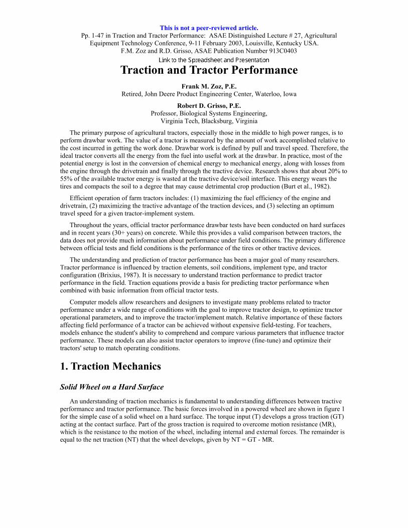
An understanding of traction mechanics is fundamental to understanding differences between tractive performance and tractor performance. The basic forces involved in a powered wheel are shown in figure 1 for the simple case of a solid wheel on a hard surface. The torque input (T) develops a gross traction (GT) acting at the contact surface. Part of the gross traction is required to overcome motion resistance (MR), which is the resistance to the motion of the wheel, including internal and external forces. The remainder is equal to the net traction (NT) that the wheel develops, given by NT = GT - MR.

http://bsesrv214.bse.vt.edu/Dist_Lecture_27

Jason Hughes

Line

GT MR

slr rr

N T T

W

Va

Wd

rt

ϖ

W = Weight, static Wd = Weight, dynamic slr = Loaded radius, static rr = Rolling radius rt = Torque radius Vt = Velocity, theoretical Va = Velocity, actual T = Axle torqueGTNTMR

GT MR

slr rr

N T T

W

Va

Wd

rt

ϖ

W Wdslr rr rt Vt Va T GT = Gross traction (theoretical pull) NT = Net traction (actual pull) MR = Motion resistance

Figure 1. Basic wheel forces for a solid wheel on a hard surface.

Soft Wheel on a Hard Surface

A soft wheel on a hard surface (fig. 2) is much the same as a solid wheel except that it becomes more obvious that the vertical reaction force (Wd) is not directly under the axle centerline but is offset by a distance designated "eh." This offset is necessary for static equilibrium. The amount of the offset is a function of the motion resistance and is given by:

( )( )Wd

MRslr eh = (1)

Three radii are shown in figures 1 and 2: "slr" is the static loaded radius, defined as the distance from the axle centerline to a hard surface; "rr" is the rolling radius, used for speed calculations. Rolling radius is derived from the rolling circumference (usually measured prior to a test but also included in tire manufacturer data tables). Static loaded radius and rolling radius are close but not equal. For a properly inflated agricultural tire, the rolling radius is about 6% greater than the static loaded radius. Rolling radius should be used for speed calculations. Static loaded radius is more appropriate to use for force or moment calculations. Both can be affected by the softness of the soil surface and are usually determined on a hard surface.

The third radius shown in figure 1 is called the torque radius (rt). This is the effective radius where the gross traction (GT) and motion resistance (MR) forces act. It cannot be measured directly but can be determined by back calculating using energy calculations. This is explained in detail in section 2 of this paper under "Gross Traction Ratio."

6

MR

slr rr

NT T

W

Va

Wd

GT

eh

rt

ϖ

W = Weight, staticWd = Weight, dynamic slr = Loaded radius, static rr = Rolling radiusrt = Torque radiusVt = Velocity, theoretical Va = Velocity, actual T = Axle torqueGT = Gross traction (theoretical pull) NT = Net traction (actual pull) MR = Motion resistance

MR

slr rr

NT T

W

Va

Wd

GT

eh

rt

ϖ

W Wdslr rr rt Vt Va T GTNTMR

Figure 2. Basic wheel forces for a soft wheel on a hard surface.

Deformable Wheel on a Soft Surface

In the real world, both the wheel and the (soil) surface are deformable and result in the forces and moments shown in figure 3. The result is both a vertical and a horizontal offset, designated "ev" and "eh," respectively. The amount of the offsets depends on the motion resistance force (MR), the tire loaded radius (slr), and the vertical force resultant (Wd):

( )( )Wd

MRev -slr eh = (2)

slr rr

NT T

W

Va

GT

Wd

eh

MR

ev Ground Line Ground Line

rt

ϖ

W = Weight, static Wd = Weight, dynamic slr = Loaded radius, static rr = Rolling radius rt = Torque radius Vt = Velocity, theoretical Va = Velocity, actual T = Axle torqueGT = Gross traction (theoretical pull) NT = Net traction (actual pull) MR = Motion resistance

slr rr

NT T

W

Va

GT

Wd

eh

MR

ev Ground Line Ground Line

rt

ϖ

W Wdslr rr rt Vt Va T GTNTMR

Figure 3. Deformable wheel on a soft surface.

7

Belt Drives

The mechanics of the belt drive mechanism (fig. 4) is similar to the wheel in many respects; but the distribution of the load is dependent on vehicle parameters. The location of the dynamic load resultant, "eh" (dynamic balance ratio; Corcoran and Gove, 1985), depends on the static distribution, the design of the suspension mechanism supporting the bogie wheels, and vehicle weight transfer characteristics.

MR

slr rr NT T

W 1

Va

Wd

GT

W2 W3 W4W5

Ground Line Dh rt

ϖ

Vt = Velocity, theoretical Va = Velocity, actual T = Axle torqueGT = Gross traction (theoretical pull) NT = Net traction (actual pull) MR = Motion resistance

W = Weight, staticWd = Weight, dynamicslr = Loaded radius, staticrr = Rolling radiusrt = Torque radius

Vt Va T GTNTMR

W Wdslr rr rt

eh Figure 4. Belt drive.

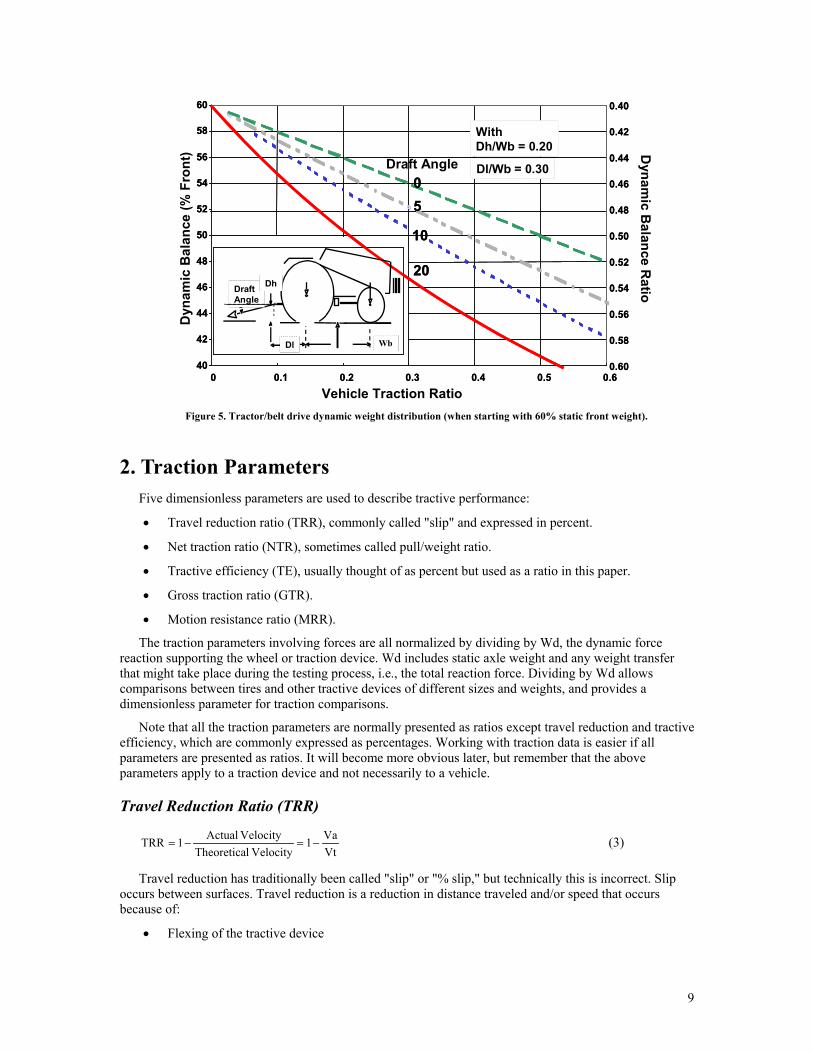
In general, the best tractive performance and the most uniform ground pressure on a belt drive can be obtained with a dynamic balance ratio of near 50%. Corcoran and Gove (1985) defined dynamic balance ratio as the ratio of the location of the vertical component of the dynamic load (external loads and tractor weight) from the front of the track divided by the track base length. Unlike a tire, where only the total dynamic weight (Wd) must be considered during a traction test, the dynamic balance of a track mechanism must be considered either in a belt test or a full vehicle test. The dynamic balance ratio obtained depends not only on tractor dimensional parameters and the location and angle of the line of draft but also on the magnitude of the drawbar pull.

Figure 5 shows the effect of draft angle and vehicle traction ratio on the dynamic balance for a tractor with 60% of the static weight at the front. A generic wheel/belt tractor is shown for simplicity, but the weight transfer mechanics are the same for belted and wheel tractors. Note that it only takes a 5° draft angle to give a 50% dynamic balance ratio at a typical vehicle traction ratio of 0.40. Figure 5 is for implements hitched to the drawbar. Even higher weight transfer, and hence higher front weight requirements, may result from the use of three-point hitch equipment.

8

5

0

10

20

40

42

44

46

48

50

52

54

56

58

60

0 0.1 0.2 0.3 0.4 0.5 0.6 Vehicle Traction Ratio

Dyn

amic

Bal

ance

(% F

ront

) Draft Angle

WithDh/Wb = 0.20

Dl/Wb = 0.30

WbDl

Draft Angle

Dh

0.60

0.58

0.56

0.54

0.52

0.50

0.48

0.46

0.44

0.42

0.40

Dynam

ic Balance R

atio

5

0

10

20

40

42

44

46

48

50

52

54

56

58

60

0 0.1 0.2 0.3 0.4 0.5 0.6

WithDh/Wb = 0.20

Dl/Wb = 0.30

WbDl

Draft Angle

Dh

0.60

0.58

0.56

0.54

0.52

0.50

0.48

0.46

0.44

0.42

0.40

Figure 5. Tractor/belt drive dynamic weight distribution (when starting with 60% static front weight).

2. Traction Parameters Five dimensionless parameters are used to describe tractive performance:

• Travel reduction ratio (TRR), commonly called "slip" and expressed in percent.

• Net traction ratio (NTR), sometimes called pull/weight ratio.

• Tractive efficiency (TE), usually thought of as percent but used as a ratio in this paper.

• Gross traction ratio (GTR).

• Motion resistance ratio (MRR).

The traction parameters involving forces are all normalized by dividing by Wd, the dynamic force reaction supporting the wheel or traction device. Wd includes static axle weight and any weight transfer that might take place during the testing process, i.e., the total reaction force. Dividing by Wd allows comparisons between tires and other tractive devices of different sizes and weights, and provides a dimensionless parameter for traction comparisons.

Note that all the traction parameters are normally presented as ratios except travel reduction and tractive efficiency, which are commonly expressed as percentages. Working with traction data is easier if all parameters are presented as ratios. It will become more obvious later, but remember that the above parameters apply to a traction device and not necessarily to a vehicle.

Travel Reduction Ratio (TRR)

VtVa1

Velocity lTheoreticaVelocity Actual1TRR −=−= (3)

Travel reduction has traditionally been called "slip" or "% slip," but technically this is incorrect. Slip occurs between surfaces. Travel reduction is a reduction in distance traveled and/or speed that occurs because of:

• Flexing of the tractive device

9

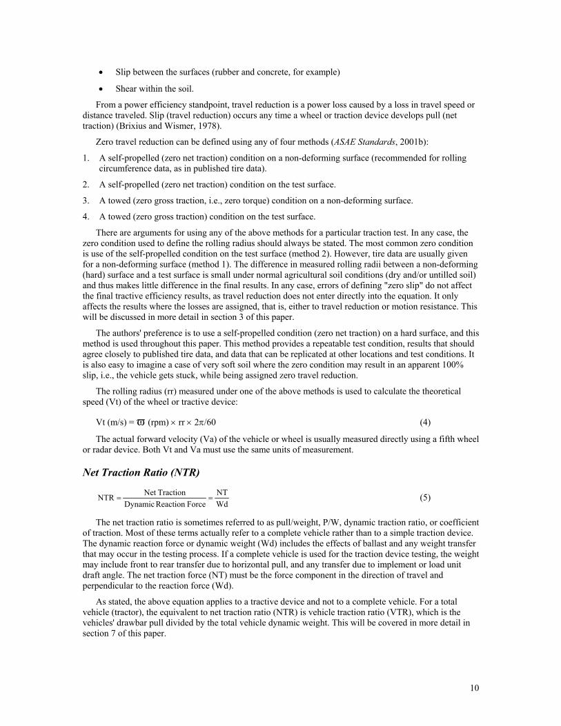
• Slip between the surfaces (rubber and concrete, for example)

• Shear within the soil.

From a power efficiency standpoint, travel reduction is a power loss caused by a loss in travel speed or distance traveled. Slip (travel reduction) occurs any time a wheel or traction device develops pull (net traction) (Brixius and Wismer, 1978).

Zero travel reduction can be defined using any of four methods (ASAE Standards, 2001b):

1. A self-propelled (zero net traction) condition on a non-deforming surface (recommended for rolling circumference data, as in published tire data).

2. A self-propelled (zero net traction) condition on the test surface.

3. A towed (zero gross traction, i.e., zero torque) condition on a non-deforming surface.

4. A towed (zero gross traction) condition on the test surface.

There are arguments for using any of the above methods for a particular traction test. In any case, the zero condition used to define the rolling radius should always be stated. The most common zero condition is use of the self-propelled condition on the test surface (method 2). However, tire data are usually given for a non-deforming surface (method 1). The difference in measured rolling radii between a non-deforming (hard) surface and a test surface is small under normal agricultural soil conditions (dry and/or untilled soil) and thus makes little difference in the final results. In any case, errors of defining "zero slip" do not affect the final tractive efficiency results, as travel reduction does not enter directly into the equation. It only affects the results where the losses are assigned, that is, either to travel reduction or motion resistance. This will be discussed in more detail in section 3 of this paper.

The authors' preference is to use a self-propelled condition (zero net traction) on a hard surface, and this method is used throughout this paper. This method provides a repeatable test condition, results that should agree closely to published tire data, and data that can be replicated at other locations and test conditions. It is also easy to imagine a case of very soft soil where the zero condition may result in an apparent 100% slip, i.e., the vehicle gets stuck, while being assigned zero travel reduction.

The rolling radius (rr) measured under one of the above methods is used to calculate the theoretical speed (Vt) of the wheel or tractive device:

Vt (m/s) = ϖ (rpm) × rr × 2π/60 (4)

The actual forward velocity (Va) of the vehicle or wheel is usually measured directly using a fifth wheel or radar device. Both Vt and Va must use the same units of measurement.

Net Traction Ratio (NTR)

WdNT

ForceReaction DynamicTractionNet NTR == (5)

The net traction ratio is sometimes referred to as pull/weight, P/W, dynamic traction ratio, or coefficient of traction. Most of these terms actually refer to a complete vehicle rather than to a simple traction device. The dynamic reaction force or dynamic weight (Wd) includes the effects of ballast and any weight transfer that may occur in the testing process. If a complete vehicle is used for the traction device testing, the weight may include front to rear transfer due to horizontal pull, and any transfer due to implement or load unit draft angle. The net traction force (NT) must be the force component in the direction of travel and perpendicular to the reaction force (Wd).

As stated, the above equation applies to a tractive device and not to a complete vehicle. For a total vehicle (tractor), the equivalent to net traction ratio (NTR) is vehicle traction ratio (VTR), which is the vehicles' drawbar pull divided by the total vehicle dynamic weight. This will be covered in more detail in section 7 of this paper.

10

Tractive Efficiency (TE)

===

×==

VtVa

GTRNTR

VtVa

WdGT

WdNT

VtVa

GTNT

Power AxleVa NT

PowerInput PowerOutput (ratio) TE

(6)

Tractive "inefficiency" is caused by both velocity losses and pull losses. The loss in travel speed is commonly referred to as "slip," although it is more accurately refered to as "travel reduction." Travel reduction is the result of the theoretical travel speed (Vt) not being entirely converted to forward progress (Va) due to losses within the soil, between the soil surface and the traction device, and within the traction device (hysteresis, and tire windup or belt slippage). Travel reduction losses are visible, that is, the operator can see it happening. The other component of tractive "inefficiency," which is less visible and often overlooked, is a loss of pull (net traction) when motion resistance reduces the amount of gross traction that is converted to useful output (net traction). This is part of what happens when a tractor is overballasted. Travel reduction is reduced, but motion resistance is increased. Motion resistance losses are especially relevant to belts, as internal losses within the belt drive mechanism, rollers, and bending of the belt are normally greater than those within a tire. On soft soils, the internal losses of belts are generally compensated for by lower external motion resistance than that of tires.

Gross Traction Ratio (GTR)

Wdrt T

WdGT GTR

×== (7)

Gross traction (GT) is sometimes referred to as rim pull, design drawbar pull, or theoretical pull. It is the axle torque input converted to a pull force. It is the pull you would develop if there were no motion resistance loss.

The gross traction ratio (GTR) is the least understood of the traction parameters. Gross traction (GT) itself cannot be measured directly and is usually calculated from the axle torque and radius of the wheel or tractive device. The problem is that the correct radius to use is not well defined or directly measurable. There is no general agreement among traction researchers as to what radius to use, and an alternate method of calculating gross traction ratio is preferred using energy or power considerations.

From equations 6 and 3:

( )TRR1TE

NTRVtVa

TENTRGTR −

=

= (8)

Having thus determined the gross traction ratio (GTR), since Wdrt T

WdGT GTR

×== ,

the effective torque radius (rt) can be calculated (although it is only of academic interest at this point to know its value) by:

( )( )WdGTRT rt = (9)

Motion Resistance Ratio (MRR)

MRR = GTR - NTR (10)

The motion resistance ratio (MRR), sometimes referred to as rolling resistance, includes internal losses within the tractive device (for example, losses within a belt drive or a tire) and soil forces. All "force" losses beyond where the torque is measured are included in motion resistance, for example, gear losses if the torque is not measured directly at the input to the tractive device. An example of this might be use of input drive shaft torque when testing tires using a mechanical front wheel drive mechanism. Rolling losses

11

of bogie wheels of a belt drive mechanism would be another example, as well as the torque required to overcome the bending of a belt.

3. Traction Data Analysis Traction data are usually normalized to create dimensionless ratios by dividing the data by the total

vertical ground reaction force (Wd). Aside from making it easier to compare tractive devices of differing sizes, the traction performance ratios make it easy to plot and compare the traction parameters for a single tractive device.

Pull Slip and NTR Slip

The most basic plot of traction data is to simply compare the pull to the travel reduction (slip). This is often the only data considered for a device where power consumption may not be a primary consideration and/or where traversing a certain terrain may be the total objective. There is also a question of which is the independent variable, pull or slip? Traction data has historically considered slip (travel reduction) to be the independent variable, that is, developing pull depends on travel reduction (slip). However, this is not unanimous, and there are reasons to believe that pull (NTR) is the independent variable and that "slip happens." Most of the data shown in this paper will consider NTR (or VTR for a complete vehicle) to be the independent variable.

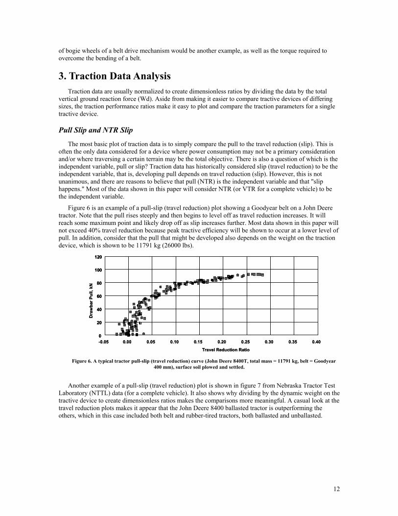
Figure 6 is an example of a pull-slip (travel reduction) plot showing a Goodyear belt on a John Deere tractor. Note that the pull rises steeply and then begins to level off as travel reduction increases. It will reach some maximum point and likely drop off as slip increases further. Most data shown in this paper will not exceed 40% travel reduction because peak tractive efficiency will be shown to occur at a lower level of pull. In addition, consider that the pull that might be developed also depends on the weight on the traction device, which is shown to be 11791 kg (26000 lbs).

0

20

40

60

80

100

120

-0.05 0.00 0.05 0.10 0.15 0.20 0.25 0.30 0.35 0.40

Travel Reduction Ratio

Dra

wba

r Pul

l,kN

0

20

40

60

80

100

120

0

20

40

60

80

100

120

-0.05 0.00 0.05 0.10 0.15 0.20 0.25 0.30 0.35 0.40


Dra

wba

r Pul

l,kN

Figure 6. A typical tractor pull-slip (travel reduction) curve (John Deere 8400T, total mass = 11791 kg, belt = Goodyear

400 mm), surface soil plowed and settled.

Another example of a pull-slip (travel reduction) plot is shown in figure 7 from Nebraska Tractor Test Laboratory (NTTL) data (for a complete vehicle). It also shows why dividing by the dynamic weight on the tractive device to create dimensionless ratios makes the comparisons more meaningful. A casual look at the travel reduction plots makes it appear that the John Deere 8400 ballasted tractor is outperforming the others, which in this case included both belt and rubber-tired tractors, both ballasted and unballasted.

12

JD 8400 MFWD Ballasted

JD 8400 MFWD Unballasted

CAT 45 Ballasted

0

5000

10000

15000

20000

25000

30000

0 2 4 6 8 10 12 14 16 Travel Reduction (%)

Dra

wba

r Pul

l (lb

s)

CAT 45 Unballasted

JD 8400 MFWD Ballasted

JD 8400 MFWD Unballasted

CAT 45 Ballasted

0

5000

10000

15000

20000

25000

30000

0 2 4 6 8 10 12 14 16

CAT 45 Unballasted

Figure 7. Nebraska test drawbar pull comparison (ballasted and unballasted).

However, dividing the pull by the weight of the vehicles, in this case the total weight on the tractive devices produces a different picture (fig. 8).

0.00

0.20

0.40

0.60

0.80

1.00

1.20

0 2 4 6 8 10 12 14 16 Travel Reduction (%)

Vehi

cle

Trac

tion

Ratio

, VTR

(pul

l / w

eigh

t)

CAT 45

JD 8400 MFWD

0.00

0.20

0.40

0.60

0.80

1.00

1.20

0 2 4 6 8 10 12 14 16

CAT 45

JD 8400 MFWD

Figure 8. Nebraska test vehicle traction ratio comparison (ballasted and unballasted).

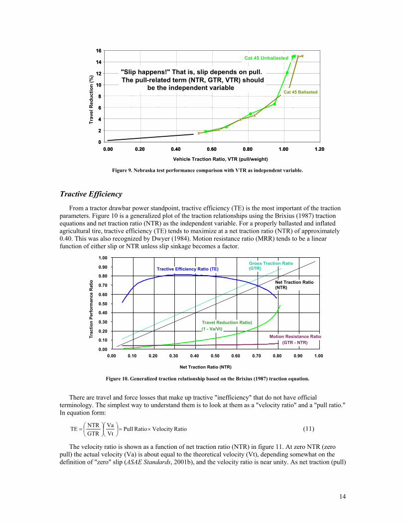
And there is still the question of which is the independent variable: travel reduction (slip), or pull (NTR or VTR)? This question cannot be answered here, as two definite groups support these two viewpoints, and each has supporting reasons. However, it is the authors' opinion that slip (travel reduction) happens because of a pull (NTR or VTR) being applied (fig. 9). This assumption will be used for the remainder of this paper.

13

0

2

4

6

8

10

12

14

16

0.00 0.20 0.40 0.60 0.80 1.00 1.20

Trav

el R

educ

tion

(%)

Vehicle Traction Ratio, VTR (pull/weight)

“Slip Happens!” That is, Slip depends upon pull. “Slip Happens!” That is, Slip depends upon pull. The pull related term, NTR, GTR, VTR should The pull related term, NTR, GTR, VTR should

be the independent variable be the independent variable

Cat 45 Unballasted

Cat 45 Ballasted

0

2

4

6

8

10

12

14

16

0.00 0.20 0.40 0.60 0.80 1.00 1.20

"Slip happens!" That is, slip depends on pull. The pull-related term (NTR, GTR, VTR) should

be the independent variable

Cat 45 Unballasted

Cat 45 Ballasted

Figure 9. Nebraska test performance comparison with VTR as independent variable.

Tractive Efficiency

From a tractor drawbar power standpoint, tractive efficiency (TE) is the most important of the traction parameters. Figure 10 is a generalized plot of the traction relationships using the Brixius (1987) traction equations and net traction ratio (NTR) as the independent variable. For a properly ballasted and inflated agricultural tire, tractive efficiency (TE) tends to maximize at a net traction ratio (NTR) of approximately 0.40. This was also recognized by Dwyer (1984). Motion resistance ratio (MRR) tends to be a linear function of either slip or NTR unless slip sinkage becomes a factor.

0.00 0.10 0.20 0.30 0.40 0.50 0.60 0.70 0.80 0.90 1.00

0.00 0.10 0.20 0.30 0.40 0.50 0.60 0.70 0.80 0.90 1.00


Trac

tion

Perfo

rman

ce R

atio


Travel Reduction Ratio)

Tractive Efficiency Ratio (TE)

(GTR - NTR) Motion Resistance Ratio

(1 - Va/Vt)

(GTR)Gross Traction Ratio

Figure 10. Generalized traction relationship based on the Brixius (1987) traction equation.

There are travel and force losses that make up tractive "inefficiency" that do not have official terminology. The simplest way to understand them is to look at them as a "velocity ratio" and a "pull ratio." In equation form:

RatioVelocity Ratio PullVtVa

GTRNTRTE ×=

= (11)

The velocity ratio is shown as a function of net traction ratio (NTR) in figure 11. At zero NTR (zero pull) the actual velocity (Va) is about equal to the theoretical velocity (Vt), depending somewhat on the definition of "zero" slip (ASAE Standards, 2001b), and the velocity ratio is near unity. As net traction (pull)

14

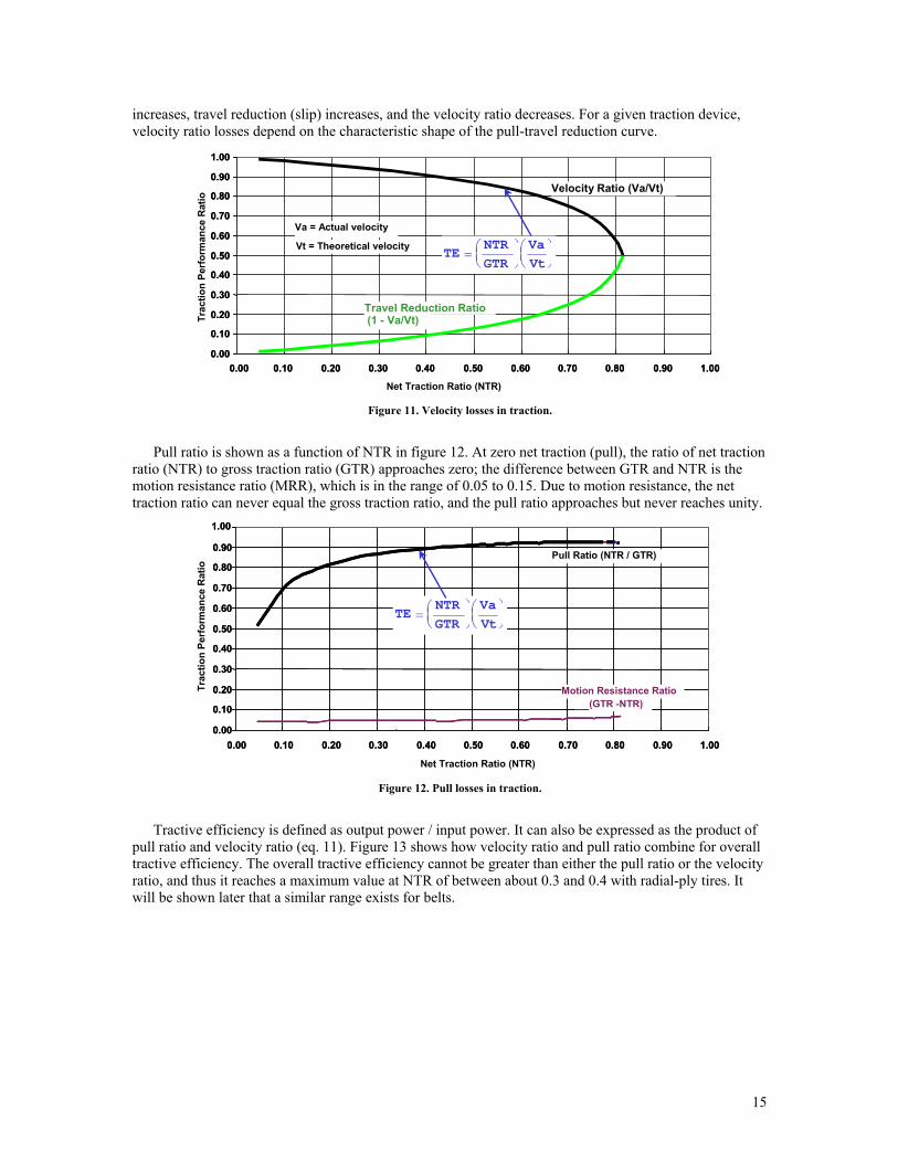
increases, travel reduction (slip) increases, and the velocity ratio decreases. For a given traction device, velocity ratio losses depend on the characteristic shape of the pull-travel reduction curve.

Va/ Vt

Travel Reduction Ratio = (1-Va/Vt)

0.00 0.10 0.20 0.30 0.40 0.50 0.60 0.70 0.80 0.90 1.00

0.00 0.10 0.20 0.30 0.40 0.50 0.60 0.70 0.80 0.90 1.00 Net Traction Ratio (NTR)

Trac

tion

Perf

orm

ance

Rat

io

Va = Actual VelocityVt = Theoretical Velocity

TENTR

GTR

Va

Vt=


0.00 0.10 0.20 0.30 0.40 0.50 0.60 0.70 0.80 0.90 1.00

0.00 0.10 0.20 0.30 0.40 0.50 0.60 0.70 0.80 0.90 1.00

Va = Actual velocity

Vt = Theoretical velocityTE

NTR

GTR

Va

Vt=

Velocity Ratio (Va/Vt)

(1 - Va/Vt)

Figure 11. Velocity losses in traction.

Pull ratio is shown as a function of NTR in figure 12. At zero net traction (pull), the ratio of net traction ratio (NTR) to gross traction ratio (GTR) approaches zero; the difference between GTR and NTR is the motion resistance ratio (MRR), which is in the range of 0.05 to 0.15. Due to motion resistance, the net traction ratio can never equal the gross traction ratio, and the pull ratio approaches but never reaches unity.

Motion Resistance Ratio - NTR

0.00 0.10 0.20 0.30 0.40 0.50 0.60 0.70 0.80 0.90 1.00


Trac

tion

Perf

orm

ance

Rat

io

Motion Resistance Ratio (GTR -NTR)

Pull Ratio (NTR / GTR)

0.00 0.10 0.20 0.30 0.40 0.50 0.60 0.70 0.80 0.90 1.00

0.00 0.10 0.20 0.30 0.40 0.50 0.60 0.70 0.80 0.90 1.00

TENTR

GTR

Va

Vt=

TENTR

GTR

Va

Vt=

Figure 12. Pull losses in traction.

Tractive efficiency is defined as output power / input power. It can also be expressed as the product of pull ratio and velocity ratio (eq. 11). Figure 13 shows how velocity ratio and pull ratio combine for overall tractive efficiency. The overall tractive efficiency cannot be greater than either the pull ratio or the velocity ratio, and thus it reaches a maximum value at NTR of between about 0.3 and 0.4 with radial-ply tires. It will be shown later that a similar range exists for belts.

15

Tractive Efficiency Ratio

Velocity Ratio = Va / Vt

Travel Reduction Ratio = (1 -Va/Vt)

Ratio = GTR - NTR

Maximum Efficiency Point

Pull Ratio = NTR / GTR

0.00 0.10 0.20 0.30 0.40 0.50 0.60 0.70 0.80 0.90 1.00


Trac

tion

Perf

orm

ance

Rat

io

TE NTR GTR

Va Vt

=




Motion Resistance Ratio (GTR - NTR)

Maximum Efficiency Point


0.00 0.10 0.20 0.30 0.40 0.50 0.60 0.70 0.80 0.90 1.00

0.00 0.10 0.20 0.30 0.40 0.50 0.60 0.70 0.80 0.90 1.00

TE NTR GTR

Va Vt

=

(1 - Va/Vt)

Figure 13. Overall tractive efficiency with velocity and pull losses.

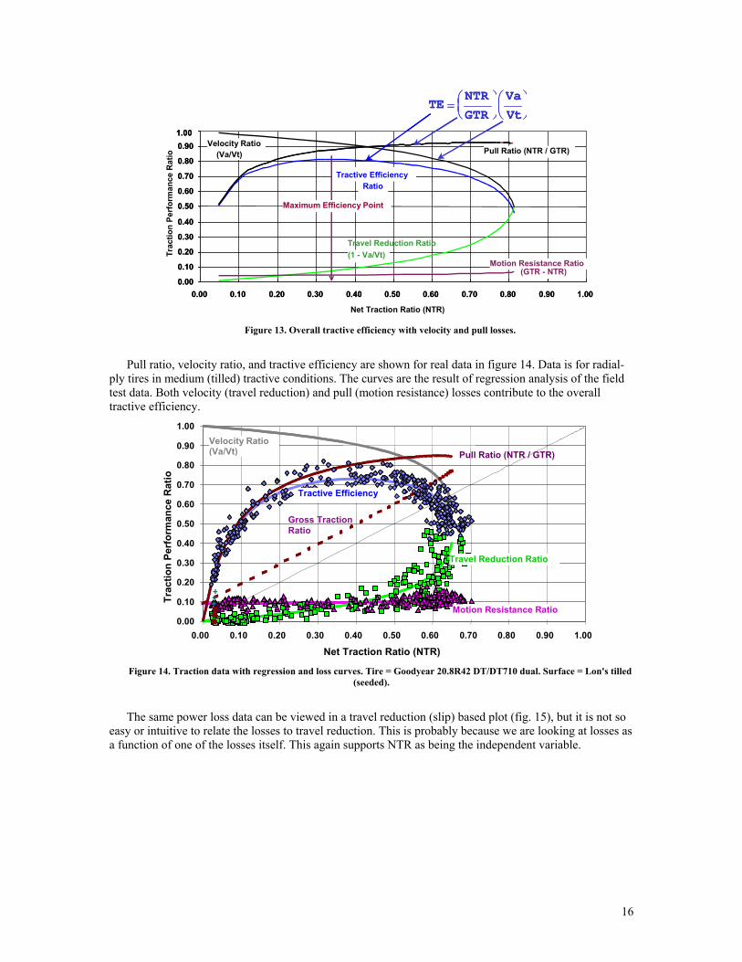
Pull ratio, velocity ratio, and tractive efficiency are shown for real data in figure 14. Data is for radial-ply tires in medium (tilled) tractive conditions. The curves are the result of regression analysis of the field test data. Both velocity (travel reduction) and pull (motion resistance) losses contribute to the overall tractive efficiency.

0.00

0.10

0.20

0.30

0.40

0.50

0.60

0.70

0.80

0.90

1.00

0.00 0.10 0.20 0.30 0.40 0.50 0.60 0.70 0.80 0.90 1.00


Trac

tion

Perf

orm

ance

Rat

io

Gross TractionRatio



Motion Resistance Ratio


Tractive Efficiency

Figure 14. Traction data with regression and loss curves. Tire = Goodyear 20.8R42 DT/DT710 dual. Surface = Lon's tilled

(seeded).

The same power loss data can be viewed in a travel reduction (slip) based plot (fig. 15), but it is not so easy or intuitive to relate the losses to travel reduction. This is probably because we are looking at losses as a function of one of the losses itself. This again supports NTR as being the independent variable.

16

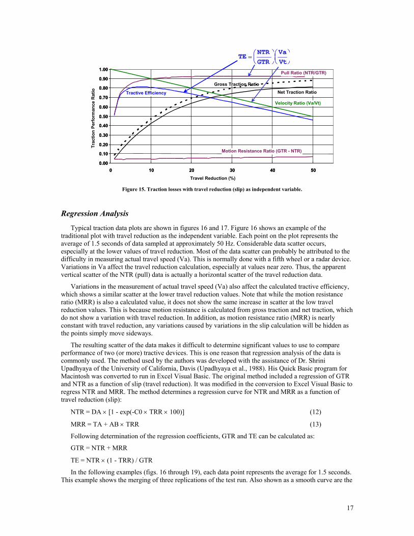
Tractive Efficiency Net Traction Ratio Gross Traction Ratio

Pull Ratio = NTR/GTR

0.00 0.10 0.20 0.30 0.40 0.50 0.60 0.70 0.80 0.90 1.00

0 10 20 30 40 50 Travel Reduction (%)

Trac

tion

Perf

orm

ance

Rat

io

Velocity Ratio = Va /Vt

TENTR

GTR

Va

Vt=

Motion Resistance Ratio = GTR - NTR

Tractive Efficiency Net Traction Ratio Gross Traction Ratio

Pull Ratio (NTR/GTR)

0.00 0.10 0.20 0.30 0.40 0.50 0.60 0.70 0.80 0.90 1.00

0 10 20 30 40 50


TENTR

GTR

Va

Vt=

Motion Resistance Ratio (GTR - NTR)

Figure 15. Traction losses with travel reduction (slip) as independent variable.

Regression Analysis

Typical traction data plots are shown in figures 16 and 17. Figure 16 shows an example of the traditional plot with travel reduction as the independent variable. Each point on the plot represents the average of 1.5 seconds of data sampled at approximately 50 Hz. Considerable data scatter occurs, especially at the lower values of travel reduction. Most of the data scatter can probably be attributed to the difficulty in measuring actual travel speed (Va). This is normally done with a fifth wheel or a radar device. Variations in Va affect the travel reduction calculation, especially at values near zero. Thus, the apparent vertical scatter of the NTR (pull) data is actually a horizontal scatter of the travel reduction data.

Variations in the measurement of actual travel speed (Va) also affect the calculated tractive efficiency, which shows a similar scatter at the lower travel reduction values. Note that while the motion resistance ratio (MRR) is also a calculated value, it does not show the same increase in scatter at the low travel reduction values. This is because motion resistance is calculated from gross traction and net traction, which do not show a variation with travel reduction. In addition, as motion resistance ratio (MRR) is nearly constant with travel reduction, any variations caused by variations in the slip calculation will be hidden as the points simply move sideways.

The resulting scatter of the data makes it difficult to determine significant values to use to compare performance of two (or more) tractive devices. This is one reason that regression analysis of the data is commonly used. The method used by the authors was developed with the assistance of Dr. Shrini Upadhyaya of the University of California, Davis (Upadhyaya et al., 1988). His Quick Basic program for Macintosh was converted to run in Excel Visual Basic. The original method included a regression of GTR and NTR as a function of slip (travel reduction). It was modified in the conversion to Excel Visual Basic to regress NTR and MRR. The method determines a regression curve for NTR and MRR as a function of travel reduction (slip):

NTR = DA × [1 - exp(-C0 × TRR × 100)] (12)

MRR = TA + AB × TRR (13)

Following determination of the regression coefficients, GTR and TE can be calculated as:

GTR = NTR + MRR

TE = NTR × (1 - TRR) / GTR

In the following examples (figs. 16 through 19), each data point represents the average for 1.5 seconds. This example shows the merging of three replications of the test run. Also shown as a smooth curve are the

17

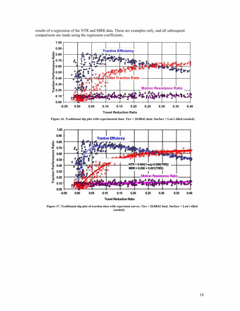
results of a regression of the NTR and MRR data. These are examples only, and all subsequent comparisons are made using the regression coefficients.

0.00 0.10 0.20 0.30 0.40 0.50 0.60 0.70 0.80 0.90 1.00

-0.05 0.00 0.05 0.10 0.15 0.20 0.25 0.30 0.35 0.40 Travel Reduction Ratio

Trac

tion

Perf

orm

ance

Rat

io Tractive Efficiency


Net Traction Ratio

Net Traction Ratio

Figure 16. Traditional slip plot with experimental data. Tire = 20.8R42 dual. Surface = Lon's tilled (seeded).

1.00

-0.05 0.00 0.05 0.10 0.15 0.20 0.25 0.30 0.35 0.40


0.00

0.10

0.20

0.30

0.40

0.50

0.60

0.70

0.80

0.90

Trac

tion

Perf

orm

ance

Rat

io

NTR = 0.664(1-exp-0.098(TRR)) MRR = 0.090 + 0.001(TRR))


Tractive Efficiency

Figure 17. Traditional slip plot of traction data with regression curves. Tire = 20.8R42 dual. Surface = Lon's tilled

(seeded).

18

0.00

0.10

0.20

0.30

0.40

0.50

0.60

0.70

0.80

0.90

1.00

0.00 0.10 0.20 0.30 0.40 0.50 0.60 0.70 0.80 0.90 1.000.00 0.10 0.20 0.30 0.40 0.50 0.60 0.70 0.80 0.90 1.00

Net Traction Ratio, NTR

Trac

tion

Perf

orm

ance

Rat

io

Tractive Efficiency



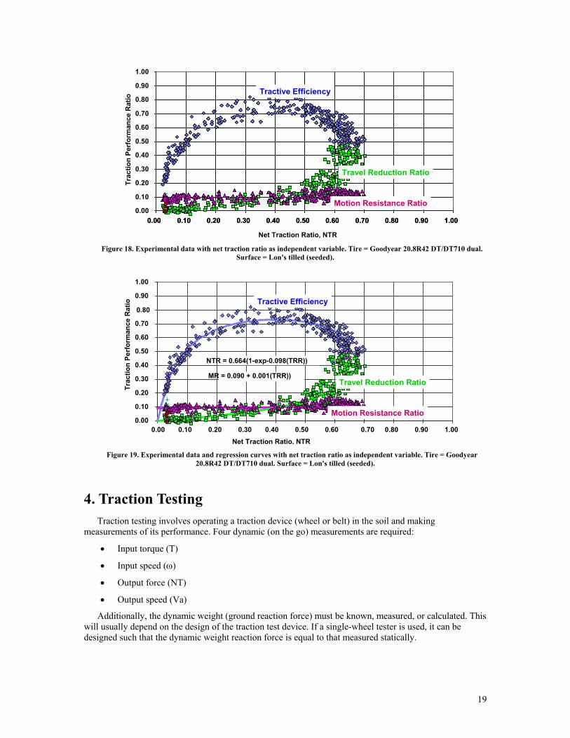
Figure 18. Experimental data with net traction ratio as independent variable. Tire = Goodyear 20.8R42 DT/DT710 dual.

Surface = Lon's tilled (seeded).

0.00 0.10 0.20 0.30 0.40 0.50 0.60 0.70 0.80 0.90 1.00Net Traction Ratio, NTR

0.00

0.10

0.20

0.30

0.40

0.50

0.60

0.70

0.80

0.90

1.00

Trac

tion

Perf

orm

ance

Rat

io

NTR = 0.664(1-exp-0.098(TRR))

MR = 0.090 + 0.001(TRR))

Tractive Efficiency



Figure 19. Experimental data and regression curves with net traction ratio as independent variable. Tire = Goodyear

20.8R42 DT/DT710 dual. Surface = Lon's tilled (seeded).

4. Traction Testing Traction testing involves operating a traction device (wheel or belt) in the soil and making

measurements of its performance. Four dynamic (on the go) measurements are required:

• Input torque (T)

• Input speed (ω)

• Output force (NT)

• Output speed (Va)

Additionally, the dynamic weight (ground reaction force) must be known, measured, or calculated. This will usually depend on the design of the traction test device. If a single-wheel tester is used, it can be designed such that the dynamic weight reaction force is equal to that measured statically.

19

Single-Wheel Testing

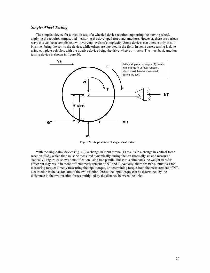
The simplest device for a traction test of a wheeled device requires supporting the moving wheel, applying the required torque, and measuring the developed force (net traction). However, there are various ways this can be accomplished, with varying levels of complexity. Some devices can operate only in soil bins, i.e., bring the soil to the device, while others are operated in the field. In some cases, testing is done using complete vehicles, with the tractive device being the drive wheels or tracks. The most basic traction testing device is shown in figure 20.

GT MR

slr rr

NT T

W

Va ω

Wd

rt

GT MR

slr rr

NT T

W

Va ω

Wd

With a single arm, torque (T) results in a change in vertical reaction, which must then be measured during the test.

rt

Figure 20. Simplest form of single-wheel tester.

With the single-link device (fig. 20), a change in input torque (T) results in a change in vertical force reaction (Wd), which then must be measured dynamically during the test (normally set and measured statically). Figure 21 shows a modification using two parallel links; this eliminates the weight transfer effect but may result in more difficult measurement of NT and T. Actually, there are two alternatives for measuring torque: directly measuring the input torque, or determining torque from the measurement of NT. Net traction is the vector sum of the two reaction forces; the input torque can be determined by the difference in the two reaction forces multiplied by the distance between the links.

20

GT MR

slr rr

T

W

Va ω

Wd

NT/2

With parallel arms, there is no change in vertical reaction as torque is applied.

NT/2

Net traction can be calculated as the sum of the reaction forces. Torque can be calculated as the difference in the forces multiplied by the distance between the arms.

rt

GT MR

slr rr

T

W

Va ω

Wd

NT/2

NT/2

rt

Figure 21. Single-wheel tester with parallel arms.

Most single-wheel testers use the mechanism shown in figure 22. Torque is measured at the input to the wheel.

GT MR

slr rr

TW

Va ω

Wd

With parallel arms, there is no change in vertical reaction as torque is applied (i.e., W = Wd)

NTrt

GT MR

slr rr

TW

Va ω

Wd

NTrt

Figure 22. Parallel arm single-wheel tester with direct measurement of NT.

Using Tractors to Test Tires

While single-wheel testing is conceptually the most simple and direct approach to testing a traction device, a tractor can be used to test tires (fig. 23) and in fact is the most common method to test belts. Use of a tractor means that two of the traction devices are actually under test. When a tractor is used, some method must be used to determine the dynamic weight on the drive wheels (due to weight transfer when pulling), and in the case of full four-wheel drive, some method must be used to determine the net traction

21

(pull) developed by each axle. For a tractor with mechanical front-wheel drive, it is nearly impossible to conduct a pure traction test because the dynamic weights and the net traction developed by the front axle need to be determined, and the front and rear axles are typically equipped with different size tires.

c

MR

slrrr T

RWS

ω

GT

Va

FWS

MRf

RWDWb

P

Dh

FWD

rt

c

MR

slrrr T

RWS

ω

GT

Va

MRf

RWDWb

P

Dh

FWD

rt

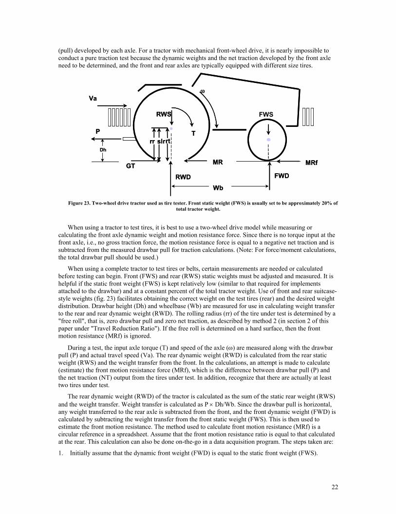
Figure 23. Two-wheel drive tractor used as tire tester. Front static weight (FWS) is usually set to be approximately 20% of

total tractor weight.

When using a tractor to test tires, it is best to use a two-wheel drive model while measuring or calculating the front axle dynamic weight and motion resistance force. Since there is no torque input at the front axle, i.e., no gross traction force, the motion resistance force is equal to a negative net traction and is subtracted from the measured drawbar pull for traction calculations. (Note: For force/moment calculations, the total drawbar pull should be used.)

When using a complete tractor to test tires or belts, certain measurements are needed or calculated before testing can begin. Front (FWS) and rear (RWS) static weights must be adjusted and measured. It is helpful if the static front weight (FWS) is kept relatively low (similar to that required for implements attached to the drawbar) and at a constant percent of the total tractor weight. Use of front and rear suitcase-style weights (fig. 23) facilitates obtaining the correct weight on the test tires (rear) and the desired weight distribution. Drawbar height (Dh) and wheelbase (Wb) are measured for use in calculating weight transfer to the rear and rear dynamic weight (RWD). The rolling radius (rr) of the tire under test is determined by a "free roll", that is, zero drawbar pull and zero net traction, as described by method 2 (in section 2 of this paper under "Travel Reduction Ratio"). If the free roll is determined on a hard surface, then the front motion resistance (MRf) is ignored.

During a test, the input axle torque (T) and speed of the axle (ω) are measured along with the drawbar pull (P) and actual travel speed (Va). The rear dynamic weight (RWD) is calculated from the rear static weight (RWS) and the weight transfer from the front. In the calculations, an attempt is made to calculate (estimate) the front motion resistance force (MRf), which is the difference between drawbar pull (P) and the net traction (NT) output from the tires under test. In addition, recognize that there are actually at least two tires under test.

The rear dynamic weight (RWD) of the tractor is calculated as the sum of the static rear weight (RWS) and the weight transfer. Weight transfer is calculated as P × Dh/Wb. Since the drawbar pull is horizontal, any weight transferred to the rear axle is subtracted from the front, and the front dynamic weight (FWD) is calculated by subtracting the weight transfer from the front static weight (FWS). This is then used to estimate the front motion resistance. The method used to calculate front motion resistance (MRf) is a circular reference in a spreadsheet. Assume that the front motion resistance ratio is equal to that calculated at the rear. This calculation can also be done on-the-go in a data acquisition program. The steps taken are:

1. Initially assume that the dynamic front weight (FWD) is equal to the static front weight (FWS).

22

2. Assume a front motion resistance ratio (MRR) as a starting point.

3. Calculate front motion resistance force (MRf) and add it to the net traction force (initially equal to drawbar pull).

4. Recalculate the new rear MRR (from within the traction calculations using new NTR).

5. Use the newly calculated rear MRR to calculate the new front (MRf).

6. Loop back until the data do not change (to whatever significance you are operating, usually the third decimal place). At this point, the front MRR is equal to the rear MRR, and the net traction force has been adjusted for what it is estimated to be required to push the front wheels through the field. Note that this means that net traction will be higher than the measured drawbar pull (considering the number of tires under test).

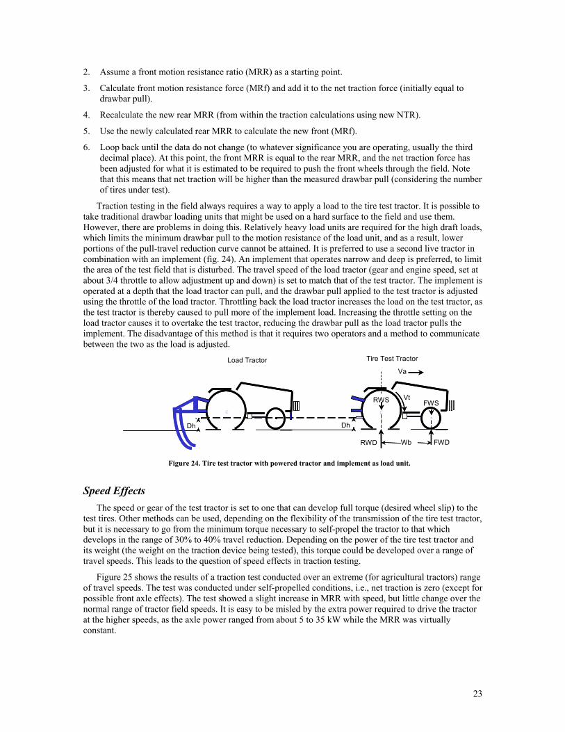
Traction testing in the field always requires a way to apply a load to the tire test tractor. It is possible to take traditional drawbar loading units that might be used on a hard surface to the field and use them. However, there are problems in doing this. Relatively heavy load units are required for the high draft loads, which limits the minimum drawbar pull to the motion resistance of the load unit, and as a result, lower portions of the pull-travel reduction curve cannot be attained. It is preferred to use a second live tractor in combination with an implement (fig. 24). An implement that operates narrow and deep is preferred, to limit the area of the test field that is disturbed. The travel speed of the load tractor (gear and engine speed, set at about 3/4 throttle to allow adjustment up and down) is set to match that of the test tractor. The implement is operated at a depth that the load tractor can pull, and the drawbar pull applied to the test tractor is adjusted using the throttle of the load tractor. Throttling back the load tractor increases the load on the test tractor, as the test tractor is thereby caused to pull more of the implement load. Increasing the throttle setting on the load tractor causes it to overtake the test tractor, reducing the drawbar pull as the load tractor pulls the implement. The disadvantage of this method is that it requires two operators and a method to communicate between the two as the load is adjusted.

c

RWS

Va

FWS

RWD FWD

Tire Test Tractor

Vt

Dh

c

Load Tractor

Dh cc

Wb

Figure 24. Tire test tractor with powered tractor and implement as load unit.

Speed Effects The speed or gear of the test tractor is set to one that can develop full torque (desired wheel slip) to the

test tires. Other methods can be used, depending on the flexibility of the transmission of the tire test tractor, but it is necessary to go from the minimum torque necessary to self-propel the tractor to that which develops in the range of 30% to 40% travel reduction. Depending on the power of the tire test tractor and its weight (the weight on the traction device being tested), this torque could be developed over a range of travel speeds. This leads to the question of speed effects in traction testing.

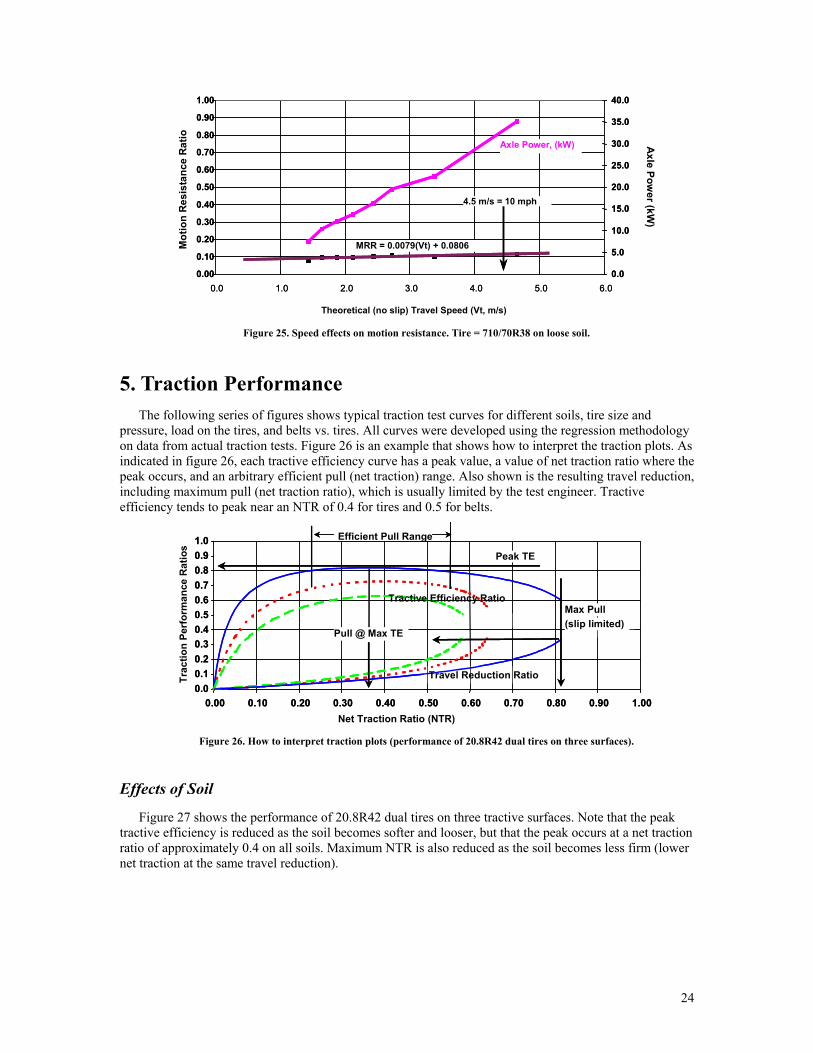
Figure 25 shows the results of a traction test conducted over an extreme (for agricultural tractors) range of travel speeds. The test was conducted under self-propelled conditions, i.e., net traction is zero (except for possible front axle effects). The test showed a slight increase in MRR with speed, but little change over the normal range of tractor field speeds. It is easy to be misled by the extra power required to drive the tractor at the higher speeds, as the axle power ranged from about 5 to 35 kW while the MRR was virtually constant.

23

Theoretical (no slip) Travel Speed (Vt, m/s)

Mot

ion

Resi

stan

ce R

atio

0.00 0.10 0.20 0.30 0.40 0.50 0.60 0.70 0.80 0.90 1.00

0.0 1.0 2.0 3.0 4.0 5.0 6.0 0.0 5.0 10.0 15.0 20.0 25.0 30.0 35.0 40.0

Axle Power (kW

)

0.00 0.10 0.20 0.30 0.40 0.50 0.60 0.70 0.80 0.90 1.00

0.0 1.0 2.0 3.0 4.0 5.0 6.0 0.0 5.0 10.0 15.0 20.0 25.0 30.0 35.0 40.0

Axle Power, (kW)

4.5 m/s = 10 mph

MRR = 0.0079(Vt) + 0.0806

Figure 25. Speed effects on motion resistance. Tire = 710/70R38 on loose soil.

5. Traction Performance The following series of figures shows typical traction test curves for different soils, tire size and

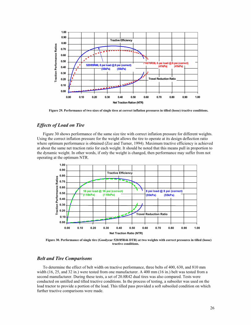
pressure, load on the tires, and belts vs. tires. All curves were developed using the regression methodology on data from actual traction tests. Figure 26 is an example that shows how to interpret the traction plots. As indicated in figure 26, each tractive efficiency curve has a peak value, a value of net traction ratio where the peak occurs, and an arbitrary efficient pull (net traction) range. Also shown is the resulting travel reduction, including maximum pull (net traction ratio), which is usually limited by the test engineer. Tractive efficiency tends to peak near an NTR of 0.4 for tires and 0.5 for belts.

Trac

tion

Perf

orm

ance

Rat

ios

0.0 0.1 0.2 0.3 0.4 0.5 0.6 0.7 0.8 0.9 1.0


Efficient Pull Range

0.0 0.1 0.2 0.3 0.4 0.5 0.6 0.7 0.8 0.9 1.0

0.00 0.10 0.20 0.30 0.40 0.50 0.60 0.70 0.80 0.90 1.00



Peak TE

Pull @ Max TE

Max Pull (slip limited)

Figure 26. How to interpret traction plots (performance of 20.8R42 dual tires on three surfaces).

Effects of Soil

Figure 27 shows the performance of 20.8R42 dual tires on three tractive surfaces. Note that the peak tractive efficiency is reduced as the soil becomes softer and looser, but that the peak occurs at a net traction ratio of approximately 0.4 on all soils. Maximum NTR is also reduced as the soil becomes less firm (lower net traction at the same travel reduction).

24

Trac

tion

Perf

orm

ance

Rat

ios

1.00


0.00 0.10 0.20 0.30 0.40 0.50 0.60 0.70 0.80 0.90

0.00 0.10 0.20 0.30 0.40 0.50 0.60 0.70 0.80 0.90 1.00


Untilled TilledSubsoiled

Tractive Efficiency

Figure 27. Performance of 20.8R42 dual tires on three surfaces (8300 kg axle load, 83 kPa tire pressure).

Effects of Tire Pressure

Figure 28 is an example of operating tires that were over-inflated for their load capacities compared to correctly inflated tires. Maximum tractive efficiency is reduced as well as the maximum net traction ratio. While the maximum tractive efficiency is only reduced about 5 percentage points, the effect on vehicle performance may be significantly greater depending on how implements are matched to the tractor. For example, at an NTR of 0.5, more than 10 percentage points of difference will result in about 17% difference in drawbar power and significantly higher travel reduction.

1.00

Trac

tion

Perf

orm

ance

Rat

ios

0.00 0.10 0.20 0.30 0.40 0.50 0.60 0.70 0.80 0.90

0.00 0.10 0.20 0.30 0.40 0.50 0.60 0.70 0.80 0.90 1.00 Net Traction Ration (NTR)

Tractive Efficiency


6 psi load @ 28 psi(41 kPa) (193 kPa)

6 psi load @ 6 psi (correct) (41 kPa) (41 kPa)

Figure 28. Performance of single tire (Firestone 710/70R38 ATR) at two inflation pressures in tilled (loose) tractive conditions.

Effects of Tire Size

Performance of two tire sizes at the correct inflation pressure is shown in figure 29. The larger diameter 520/85R46 tire shows significantly higher power efficiency at the same slip. This demonstrates that wider tires (710/70R38) have greater motion resistance loss (both operating at about the same travel reduction). Both provide similar maximum pull capability, which may give the operator the impression that there is no performance difference between the tires.

25

1.00

1.00 Net Traction Ration (NTR)

0.00 0.10 0.20 0.30 0.40 0.50 0.60 0.70 0.80 0.90

0.00 0.10 0.20 0.30 0.40 0.50 0.60 0.70 0.80 0.90

Trac

tion

Perf

orm

ance

Rat

ios

Tractive Efficiency


520/85R46, 8 psi load @ 8 psi (correct)(55kPa) (55kPa)

710/70R38, 6 psi load @ 6 psi (correct) (41kPa) (41kPa)

Figure 29. Performance of two sizes of single tires at correct inflation pressures in tilled (loose) tractive conditions.

Effects of Load on Tire

Figure 30 shows performance of the same size tire with correct inflation pressure for different weights. Using the correct inflation pressure for the weight allows the tire to operate at its design deflection ratio where optimum performance is obtained (Zoz and Turner, 1994). Maximum tractive efficiency is achieved at about the same net traction ratio for each weight. It should be noted that this means pull in proportion to the dynamic weight. In other words, if only the weight is changed, then performance may suffer from not operating at the optimum NTR.

1.00


0.00 0.10 0.20 0.30 0.40 0.50 0.60 0.70 0.80 0.90

0.00 0.10 0.20 0.30 0.40 0.50 0.60 0.70 0.80 0.90 1.00

Trac

tion

Perf

orm

ance

Rat

ios

Tractive Efficiency

16 psi load @ 16 psi (correct)(110kPa) (110kPa)

8 psi load @ 8 psi (correct) (55kPa) (55kPa)


Figure 30. Performance of single tire (Goodyear 520/85R46 DTR) at two weights with correct pressures in tilled (loose)

tractive conditions.

Belt and Tire Comparisons

To determine the effect of belt width on tractive performance, three belts of 400, 630, and 810 mm width (16, 25, and 32 in.) were tested from one manufacturer. A 400 mm (16 in.) belt was tested from a second manufacturer. During these tests, a set of 20.8R42 dual tires was also compared. Tests were conducted on untilled and tilled tractive conditions. In the process of testing, a subsoiler was used on the load tractor to provide a portion of the load. This tilled pass provided a soft subsoiled condition on which further tractive comparisons were made.

26

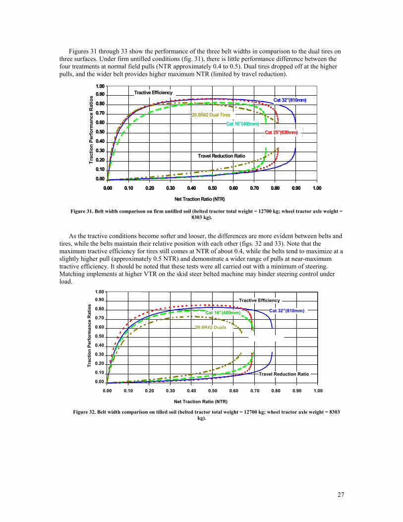
Figures 31 through 33 show the performance of the three belt widths in comparison to the dual tires on three surfaces. Under firm untilled conditions (fig. 31), there is little performance difference between the four treatments at normal field pulls (NTR approximately 0.4 to 0.5). Dual tires dropped off at the higher pulls, and the wider belt provides higher maximum NTR (limited by travel reduction).

1.00


Trac

tion

Perf

orm

ance

Rat

ios

0.00 0.10 0.20 0.30 0.40 0.50 0.60 0.70 0.80 0.90

0.00 0.10 0.20 0.30 0.40 0.50 0.60 0.70 0.80 0.90 1.00

1.00

0.00 0.10 0.20 0.30 0.40 0.50 0.60 0.70 0.80 0.90

0.00 0.10 0.20 0.30 0.40 0.50 0.60 0.70 0.80 0.90 1.00


20.8R42 Dual Tires

Tractive EfficiencyCat 32”(810mm)

Cat 16”(400mm)

Cat 25”(630mm)

Cat 25”(630mm)

Figure 31. Belt width comparison on firm untilled soil (belted tractor total weight = 12700 kg; wheel tractor axle weight = 8303 kg).

As the tractive conditions become softer and looser, the differences are more evident between belts and tires, while the belts maintain their relative position with each other (figs. 32 and 33). Note that the maximum tractive efficiency for tires still comes at NTR of about 0.4, while the belts tend to maximize at a slightly higher pull (approximately 0.5 NTR) and demonstrate a wider range of pulls at near-maximum tractive efficiency. It should be noted that these tests were all carried out with a minimum of steering. Matching implements at higher VTR on the skid steer belted machine may hinder steering control under load.

1.00

0.00 0.10 0.20 0.30 0.40 0.50 0.60 0.70 0.80 0.90


Trac

tion

Perf

orm

ance

Rat

ios

20.8R42 Duals

Cat 16”(400mm)


Cat 32”(810mm) Tractive Efficiency

Figure 32. Belt width comparison on tilled soil (belted tractor total weight = 12700 kg; wheel tractor axle weight = 8303

kg).

27

1.00

Trac

tion

Perf

orm

ance

Rat

ios

0.00 0.10 0.20 0.30 0.40 0.50 0.60 0.70 0.80 0.90


Tractive EfficiencyCat 32”(810mm)

Cat 16”(400mm)

20.8R42 Duals


Cat 25”(630mm)

GY 16”(400mm)

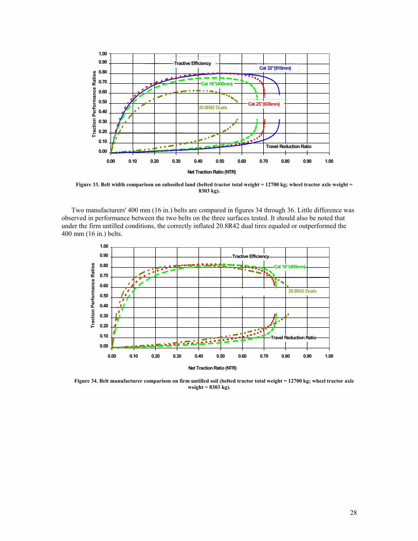
Figure 33. Belt width comparison on subsoiled land (belted tractor total weight = 12700 kg; wheel tractor axle weight = 8303 kg).

Two manufacturers' 400 mm (16 in.) belts are compared in figures 34 through 36. Little difference was observed in performance between the two belts on the three surfaces tested. It should also be noted that under the firm untilled conditions, the correctly inflated 20.8R42 dual tires equaled or outperformed the 400 mm (16 in.) belts.

1.00

0.00 0.10 0.20 0.30 0.40 0.50 0.60 0.70 0.80 0.90


Trac

tion

Perf

orm

ance

Rat

ios

Tractive Efficiency

Cat 16”(400mm)

20.8R42 Duals


Figure 34. Belt manufacturer comparison on firm untilled soil (belted tractor total weight = 12700 kg; wheel tractor axle

weight = 8303 kg).

28

1.00

Trac

tion

Perf

orm

ance

Rat

ios

0.00 0.10 0.20 0.30 0.40 0.50 0.60 0.70 0.80 0.90

0.00 0.10 0.20 0.30 0.40 0.50 0.60 0.70 0.80 0.90 1.00 Net Traction Ration (NTR)


Tractive Efficiency

20.8R42 Duals

Cat 16”(400mm)

GY 16”(400mm)

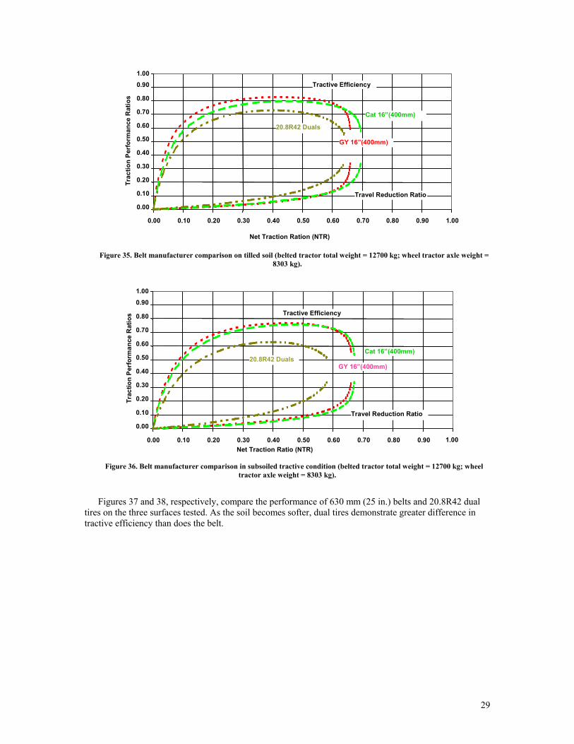
Figure 35. Belt manufacturer comparison on tilled soil (belted tractor total weight = 12700 kg; wheel tractor axle weight = 8303 kg).

1.00

1.00 Net Traction Ratio (NTR)

0.00 0.10 0.20 0.30 0.40 0.50 0.60 0.70 0.80 0.90

0.00 0.10 0.20 0.30 0.40 0.50 0.60 0.70 0.80 0.90

Trac

tion

Perf

orm

ance

Rat

ios

20.8R42 Duals

Tractive Efficiency

Cat 16”(400mm)


GY 16”(400mm)

Figure 36. Belt manufacturer comparison in subsoiled tractive condition (belted tractor total weight = 12700 kg; wheel

tractor axle weight = 8303 kg).

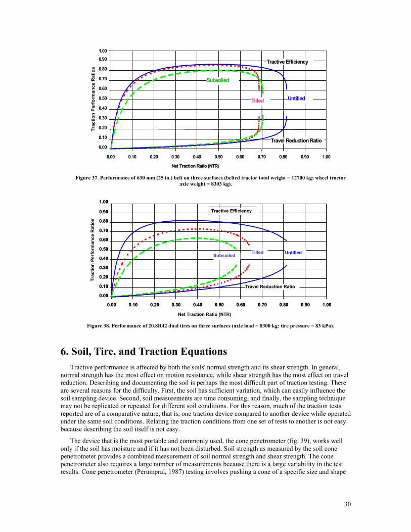
Figures 37 and 38, respectively, compare the performance of 630 mm (25 in.) belts and 20.8R42 dual tires on the three surfaces tested. As the soil becomes softer, dual tires demonstrate greater difference in tractive efficiency than does the belt.

29

1.00

Trac

tion

Perf

orm

ance

Rat

ios

0.00 0.10 0.20 0.30 0.40 0.50 0.60 0.70 0.80 0.90



Untilled

Subsoiled

Tractive Efficiency

Tilled

Figure 37. Performance of 630 mm (25 in.) belt on three surfaces (belted tractor total weight = 12700 kg; wheel tractor

axle weight = 8303 kg).

Trac

tion

Perf

orm

ance

Rat

ios

1.00


0.00 0.10 0.20 0.30 0.40 0.50 0.60 0.70 0.80 0.90

0.00 0.10 0.20 0.30 0.40 0.50 0.60 0.70 0.80 0.90 1.00

1.00

0.00 0.10 0.20 0.30 0.40 0.50 0.60 0.70 0.80 0.90

0.00 0.10 0.20 0.30 0.40 0.50 0.60 0.70 0.80 0.90 1.00


Untilled TilledSubsoiled

Tractive Efficiency

Figure 38. Performance of 20.8R42 dual tires on three surfaces (axle load = 8300 kg; tire pressure = 83 kPa).

6. Soil, Tire, and Traction Equations Tractive performance is affected by both the soils' normal strength and its shear strength. In general,

normal strength has the most effect on motion resistance, while shear strength has the most effect on travel reduction. Describing and documenting the soil is perhaps the most difficult part of traction testing. There are several reasons for the difficulty. First, the soil has sufficient variation, which can easily influence the soil sampling device. Second, soil measurements are time consuming, and finally, the sampling technique may not be replicated or repeated for different soil conditions. For this reason, much of the traction tests reported are of a comparative nature, that is, one traction device compared to another device while operated under the same soil conditions. Relating the traction conditions from one set of tests to another is not easy because describing the soil itself is not easy.

The device that is the most portable and commonly used, the cone penetrometer (fig. 39), works well only if the soil has moisture and if it has not been disturbed. Soil strength as measured by the soil cone penetrometer provides a combined measurement of soil normal strength and shear strength. The cone penetrometer also requires a large number of measurements because there is a large variability in the test results. Cone penetrometer (Perumpral, 1987) testing involves pushing a cone of a specific size and shape

30

into the soil at a certain rate and recording the resisting force exerted by the soil on the penetrometer (ASAE Standards, 2001c).

Figure 39. ASAE standard cone penetrometer for soil.

The force required to push the cone into the ground is recorded as a function of depth. The force divided by the area of the base of the cone provides a "pressure" measurement and is referred to as cone index. Common units are lb/in2 in English units and kN/m2 (megapascal) in SI units. Cone index may be measured as deep as 500 mm (20 in.) when used for tillage and/or compaction measurements, but the upper 100 to 150 mm (4 to 6 in.) is commonly used for traction purposes. The engineering practice (ASAE Standards, 2001a) provides a systemic approach for observing and presenting cone index data.

If tractive performance is to be predicted, then mathematical expressions for the interaction of the traction device and the soil must be developed. Traction equations have been developed and reported by several researchers (Wismer and Luth, 1972; Brixius, 1987; Upadhyaya et al., 1988; Zoz and Brixius, 1979), but the most commonly accepted are those reported by Brixius (1987). The equations were developed to predict the tractive performance of bias-ply tires operating in cohesive frictional soils. Tire torque, motion resistance, net traction, and tractive efficiency are predicted as a function of soil strength, tire load, travel reduction (slip), tire size, and tire deflection. As bias-ply tires are no longer in common use, modifications proposed by Brixius (1987) and verified by Al-Hamad et al. (1994) for radial-ply tires are now generally used.

The Brixius (1987) equation uses three relationships:

Mobility number:

+

+

=

db31

hδ51

WCIbdBn (14)

Torque ratio:

( )( ) 0.04e1e10.88rWQGTR 7.5S0.1Bn +−−== −− (15)

Motion resistance ratio:

31

Bn0.5S0.04

Bn1.0

WMMRR ++== (16)

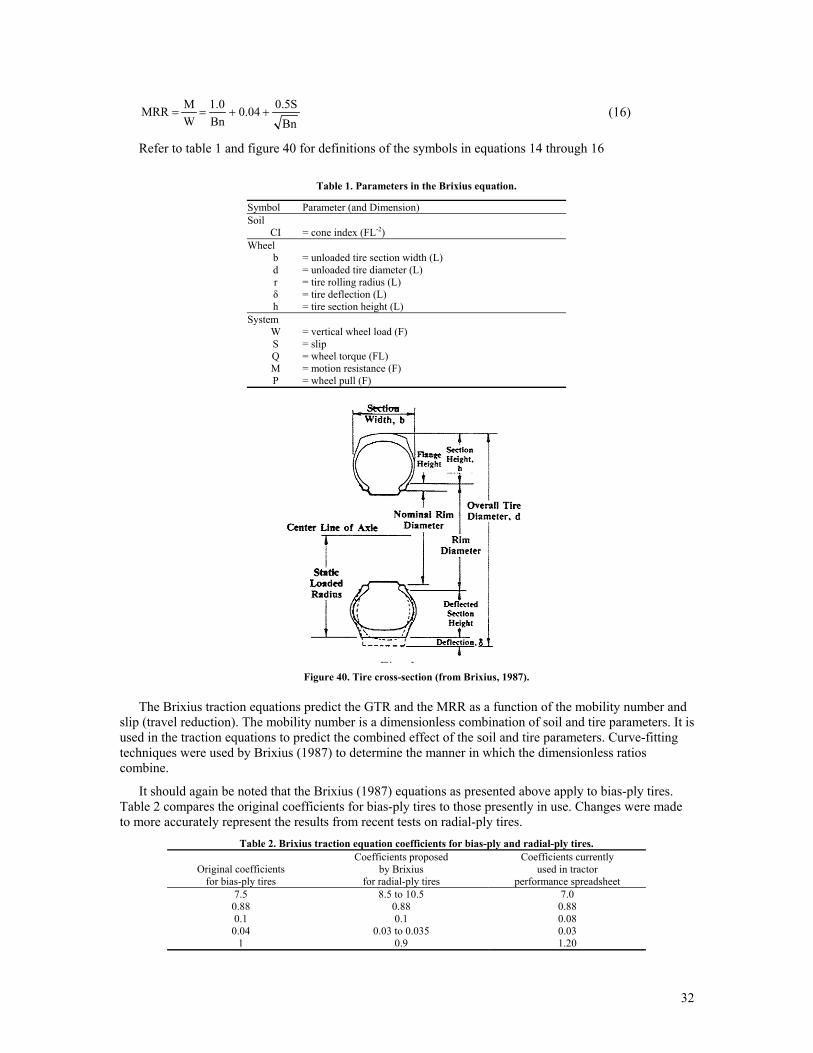
Refer to table 1 and figure 40 for definitions of the symbols in equations 14 through 16

Table 1. Parameters in the Brixius equation.

Symbol Parameter (and Dimension) Soil

CI = cone index (FL-2) Wheel

b = unloaded tire section width (L) d = unloaded tire diameter (L) r = tire rolling radius (L) δ = tire deflection (L) h = tire section height (L)

System W = vertical wheel load (F) S = slip Q = wheel torque (FL) M = motion resistance (F) P = wheel pull (F)

Figure 40. Tire cross-section (from Brixius, 1987).

The Brixius traction equations predict the GTR and the MRR as a function of the mobility number and slip (travel reduction). The mobility number is a dimensionless combination of soil and tire parameters. It is used in the traction equations to predict the combined effect of the soil and tire parameters. Curve-fitting techniques were used by Brixius (1987) to determine the manner in which the dimensionless ratios combine.

It should again be noted that the Brixius (1987) equations as presented above apply to bias-ply tires. Table 2 compares the original coefficients for bias-ply tires to those presently in use. Changes were made to more accurately represent the results from recent tests on radial-ply tires.

Table 2. Brixius traction equation coefficients for bias-ply and radial-ply tires.

Original coefficients for bias-ply tires

Coefficients proposed by Brixius

for radial-ply tires

Coefficients currently used in tractor

performance spreadsheet 7.5 8.5 to 10.5 7.0 0.88 0.88 0.88 0.1 0.1 0.08 0.04 0.03 to 0.035 0.03

1 0.9 1.20

32

Calculating tractive performance using the Brixius (1987) equations requires an iterative solution and is best handled in a computer program or spreadsheet. Calculating tractor performance adds another iterative dimension, as the dynamic weight on the tires depends on the pull (due to weight transfer), and the pull (calculated from the traction equations) depends on the weight. A spreadsheet has been developed to calculate tractor performance and is described in section 7 of this paper.

7. Tractor Performance Tractor performance is not the same as tractive performance. Tractor performance is proportional to the

performance of the traction device(s), but not equal to it. The primary difference is that tractive performance (efficiency) depends on knowing the input power (axle power) to the traction device. Axle power for a complete tractor is seldom known and is not measured during official tests. But there are also other reasons that tractive performance and tractor performance differ:

• Tractive performance is given for a defined tire or traction device, for example an 18.4R46 tire. A tractor may operate with a combination of different traction devices, that is, different size tires on the front and rear axles.

• Due to weight transfer when operating, even if a tractor has the same tires front and rear (4WD tractors, for example), both the static and dynamic weight that the tires are operating with will likely be different between the front and rear axles, requiring different tire pressures and thus a "different" traction device.

The performance of a tractor depends on the performance of a combination of traction devices and the performance of the tractor drivetrain (table 3).

Table 3. Comparison of traction device and tractor.

Traction device Tractor Axle power input Axle power usually unknown Tractive efficiency (from axle to "drawbar") Power delivery efficiency (from PTO or engine to drawbar)

Net traction (NT) Drawbar pull Net traction ratio, NTR Vehicle traction ratio (VTR) Travel reduction ratio Travel reduction ratio (but may differ at different drive wheels) Motion resistance ratio (MRR) Requires tow test to measure Gross traction ratio Not applicable; impossible to calculate Dynamic weight on device Variable between axles Single tire size May have multiple sizes Single tire pressure (at given load) May have multiple pressures Tractor size defined by PTO or engine power

While the efficiency of a traction device is defined as tractive efficiency, the efficiency of a complete tractor is defined as power delivery efficiency (Zoz et al., 2002). Power delivery efficiency (PDE) is defined as the ratio of the delivered drawbar power of a tractor to the vehicle input power of the tractor. It represents the percentage of power produced by the engine that is available as tractive power delivered through the drawbar (Shell et al., 1997; Turner et al., 1997, Zoz et al., 2002). Tractive efficiency itself is defined as the ratio of output power to input power of a traction device (ASAE Standards, 2001b). PDE includes TE and the efficiencies of the entire vehicle drivetrain from the engine to the drawbar.

PDE is computed by dividing drawbar power by a specified input power measured at some location behind the engine. Exactly where this input power is measured may vary with the specific vehicle. It is advantageous for the input power to be measured at a location that defines the power level of the tractor being tested. For many tractors, this is the power take-off (PTO). For vehicles where size is commonly specified by engine power, such as 4WD tractors or tractors without PTOs, engine flywheel power may be the only power measurement used. When engine flywheel power or axle power is used as the input, it is normally measured directly during tractor comparison testing.

When PTO power is used, it is commonly predicted during tractor comparison testing using laboratory-derived regressions from previously correlated engine parameters such as engine speed, fuel rack position, and injector needle lift duration. While power measured at different locations such as engine flywheel,

33

PTO, transmission output, or drive axles can be used in the PDE calculation, if two tractors are to be correctly compared to one another, then the power used for the PDE calculation must be measured at the same point on each tractor. It is also most meaningful if the location used is that which defines the size of the tractor, which is the advertised power.

PDE is most accurate as a comparator if the engine flywheel power can actually be measured and used in the calculation. Measured engine flywheel power is used directly in the PDE calculation as follows:

Power EnginePowerDrawbar

PDE = (17)

When it is necessary to use regression analysis or other method to determine the equivalent PTO performance, the following equation is used:

Power PTO EquivalentPowerDrawbar PDE = (18)

Power delivery efficiency depends on the performance of the PTO and transmission drivetrains as well as the performance of the tires or other traction device. Various power losses can be summarized as:

PTO power = Engine power - PTO drivetrain loss - Hydraulic loss from PTO operation.

Axle power = Engine power - Transmission drivetrain loss - Hydraulic loss from transmission operation.

Drawbar power = Axle power × tractive efficiency.

and Efficiency Drive PTO

Efficiency Tractive Efficiency Driveon TransmissiPDE ×= (19)

It becomes obvious that tractor performance depends on more than just the performance of the traction device(s).

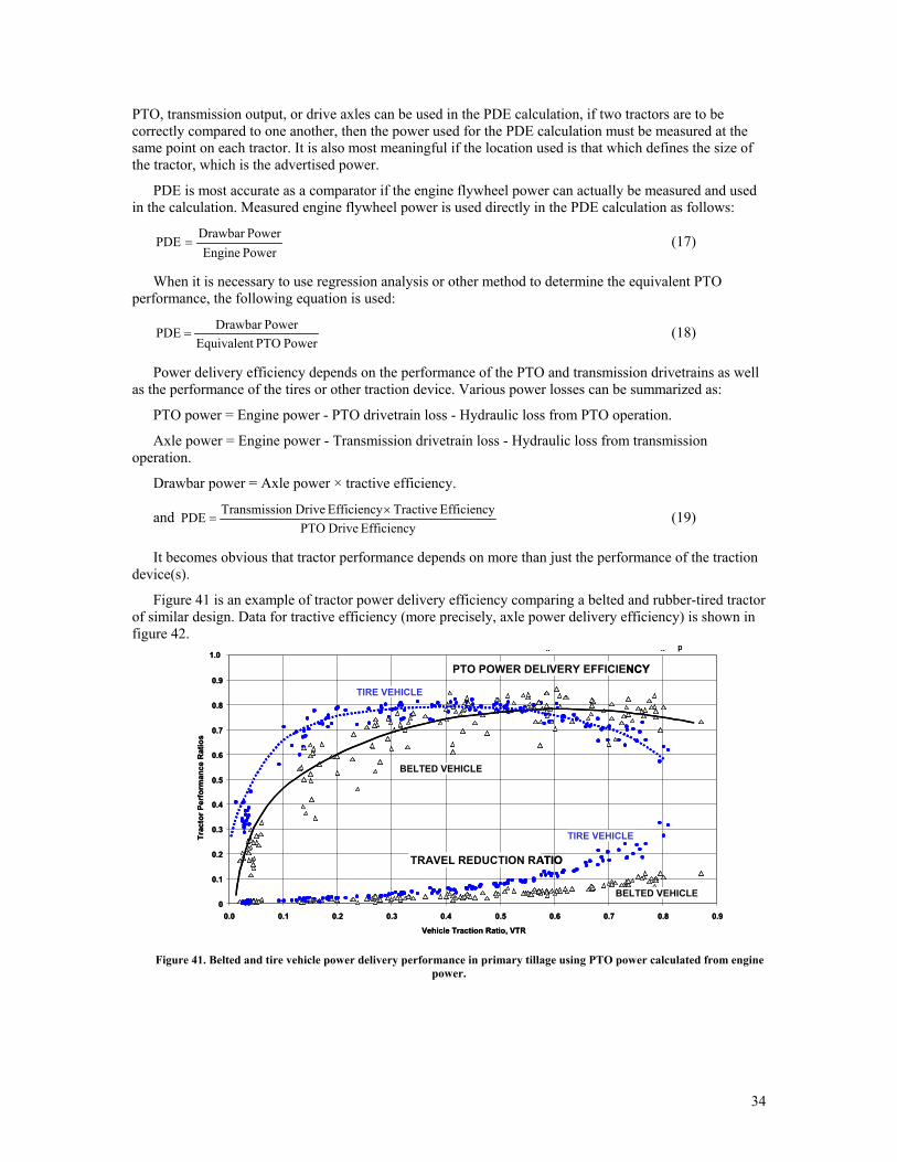
Figure 41 is an example of tractor power delivery efficiency comparing a belted and rubber-tired tractor of similar design. Data for tractive efficiency (more precisely, axle power delivery efficiency) is shown in figure 42.

0

0.1

0.2

0.3

0.4

0.5

0.6

0.7

0.8

0.9

1.0

0.0 0.1 0.2 0.3 0.4 0.5 0.6 0.7 0.8 0.9

Vehicle Traction Ratio, VTR

Trac

tor P

erfo

rman

ce R

atio

s

g g p

PTO POWER DELIVERY EFFICIENCY

TRAVEL REDUCTION RATIO

TIRE VEHICLE

BELTED VEHICLE

BELTED VEHICLE

TIRE VEHICLE

0

0.1

0.2

0.3

0.4

0.5

0.6

0.7

0.8

0.9

1.0

0.0 0.1 0.2 0.3 0.4 0.5 0.6 0.7 0.8 0.9

Vehicle Traction Ratio, VTR

Trac

tor P

erfo

rman

ce R

atio

s

g g p

PTO POWER DELIVERY EFFICIENCY


TIRE VEHICLE

BELTED VEHICLE

BELTED VEHICLE

TIRE VEHICLE

Figure 41. Belted and tire vehicle power delivery performance in primary tillage using PTO power calculated from engine

power.

34

0

0.1

0.2

0.3

0.4

0.5

0.6

0.7

0.8

0.9

1

0 0.1 0.2 0.3 0.4 0.5 0.6 0.7 0.8 0.9Vehicle Traction Ratio, VTR

Trac

tion

Perf

orm

ance

Rat

ios

TIRE

BELT TRACTIVE EFFICIENCY


BELT

TIRE

0

0.1

0.2

0.3

0.4

0.5

0.6

0.7

0.8

0.9

1

0 0.1 0.2 0.3 0.4 0.5 0.6 0.7 0.8 0.9Vehicle Traction Ratio, VTR

Trac

tion

Perf

orm

ance

Rat

ios

TIRE

BELT TRACTIVE EFFICIENCY


BELT

TIRE

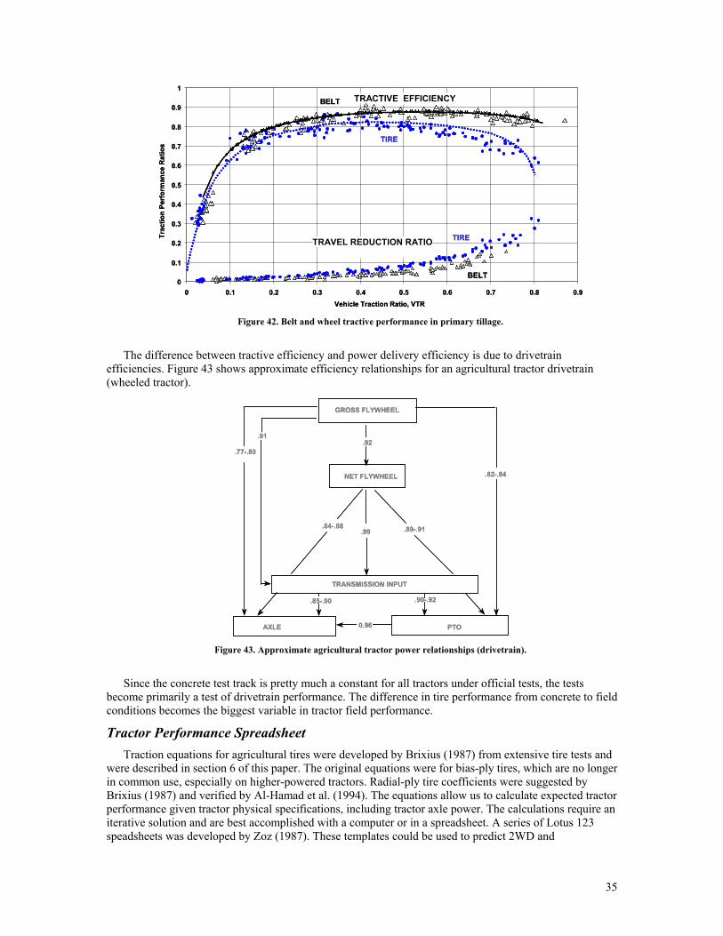
Figure 42. Belt and wheel tractive performance in primary tillage.

The difference between tractive efficiency and power delivery efficiency is due to drivetrain efficiencies. Figure 43 shows approximate efficiency relationships for an agricultural tractor drivetrain (wheeled tractor).

GROSS FLYWHEEL

NET FLYWHEEL

TRANSMISSION INPUT

AXLE PTO0.96

.85-.90 .90-.92

.77-.80

.91.92

.82-.84

.89-.91.84-.88.99

GROSS FLYWHEEL

NET FLYWHEEL

TRANSMISSION INPUT

AXLE PTO0.96

.85-.90 .90-.92

.77-.80

.91.92

.82-.84

.89-.91.84-.88.99

Figure 43. Approximate agricultural tractor power relationships (drivetrain).

Since the concrete test track is pretty much a constant for all tractors under official tests, the tests become primarily a test of drivetrain performance. The difference in tire performance from concrete to field conditions becomes the biggest variable in tractor field performance.

Tractor Performance Spreadsheet Traction equations for agricultural tires were developed by Brixius (1987) from extensive tire tests and

were described in section 6 of this paper. The original equations were for bias-ply tires, which are no longer in common use, especially on higher-powered tractors. Radial-ply tire coefficients were suggested by Brixius (1987) and verified by Al-Hamad et al. (1994). The equations allow us to calculate expected tractor performance given tractor physical specifications, including tractor axle power. The calculations require an iterative solution and are best accomplished with a computer or in a spreadsheet. A series of Lotus 123 speadsheets was developed by Zoz (1987). These templates could be used to predict 2WD and

35

4WD/MFWD tractor performance on agricultural soils. Drawbar performance including pull, speed, power, and wheel slip were calculated. An alternative calculation mode was provided to determine the required static weight necessary to obtain a given performance, i.e., a tractor weight guide. The spreadsheet was later updated to Excel and has been widely distributed in the ASAE community (fig. 44).

Figure 44. Excel spreadsheet for predicting tractor field performance under field conditions.

The spreadsheet has two modes of use, either performance calculation or tractor weight calculation; inputs and outputs change accordingly.

Common inputs (for performance calculation and weight calculation):

• Rear tire size. A data table is provided for the most common R1 tires of radial-ply or bias-ply construction. The initial value taken is that used for Nebraska Tractor Testing Laboratory (NTTL) tests when tractor is selected.

• Front tire size. A data table is provided for the most common R1 radial-ply and bias-ply tires and F2 tires for 2WD tractors. The initial value taken is that used for NTTL tests when tractor is selected.

• Number of tires. Allows use of single, dual, or triple tires. The initial value taken is that used for NTTL tests when tractor is selected.

• Tractor wheelbase. Taken from NTTL data when tractor is selected.

• Hitch height. Initially taken as the drawbar height from NTTL data when tractor is selected. However, it must be changed for other hitch configurations.

• Draft angle. The initial draft angle is zero as taken from NTTL data. However, it can be varied for drawbar operation and must be changed along with hitch height and rear location for use with hitch-mounted implements.

• Hitch location behind rear axle. This data is not given by NTTL and is not necessary for operation with horizontal drawbar pull. The spreadsheet automatically inserts nominal values (that can be changed) when implement type is selected.

36

• Input power. Axle power is used by the spreadsheet. However, as stated earlier, axle power is seldom known for a tractor, even from official tests. The spreadsheet uses an input power and a transmission efficiency to calculate axle power. A tractor database is provided which takes data from NTTL tests. The efficiency of power transmission from PTO or engine to axle has been calculated from NTTL data by back calculation, assuming tire efficiency on concrete of 92.5%. This value was taken from extensive traction tests of tires on concrete. It results from approximately 2% motion resistance and 5% travel reduction at maximum tractive efficiency. Input power is split between front and rear on 4WD/MFWD tractors by the dynamic weight and wheel mobility number.

• Travel speed, theoretical (Vt). The initial value is 5 mph, which probably should be changed. The theoretical speed is the speed without travel reduction and is the speed that is normally given in tractor specifications for a tire of a given size. If a tractor is equipped with radar, it is the speed that would be measured without slip (travel reduction) at the appropriate engine speed.

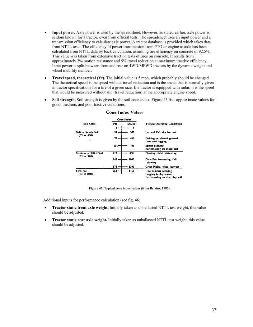
• Soil strength. Soil strength is given by the soil cone index. Figure 45 lists approximate values for good, medium, and poor tractive conditions.

Figure 45. Typical cone index values (from Brixius, 1987).

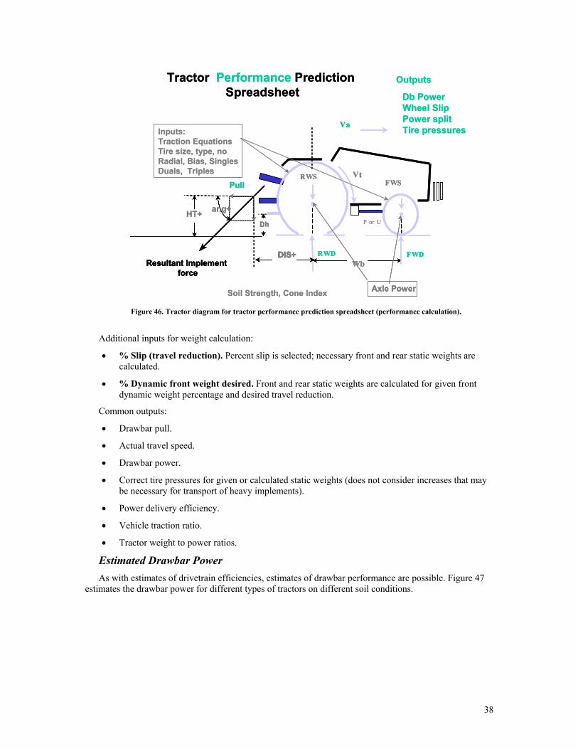
Additional inputs for performance calculation (see fig. 46):

• Tractor static front axle weight. Initially taken as unballasted NTTL test weight, this value should be adjusted.

• Tractor static rear axle weight. Initially taken as unballasted NTTL test weight, this value should be adjusted.

37

Resultant Implement force

c

Va

FWSRWS

RWDWb

FWD

HT+

DIS+

ang+

Tractor Performance PredictionSpreadsheet

Vt

Dh

Pull

Inputs:Traction EquationsTire size, type, noRadial, Bias, SinglesDuals, Triples

Soil Strength, Cone Index

Db PowerWheel SlipPower splitTire pressures

P or U

DIS+

Outputs

Axle Power




c

VaVa

FWSFWSRWSRWS

RWDRWDWbWb

FWDFWD

HT+HT+

DIS+DIS+

ang+ang+

Tractor Performance PredictionSpreadsheet

VtVt

DhDh

PullPull

Inputs:Traction EquationsTire size, type, noRadial, Bias, SinglesDuals, Triples

Soil Strength, Cone Index

Db PowerWheel SlipPower splitTire pressures

P or U

DIS+DIS+

Outputs

Axle PowerAxle Power

Figure 46. Tractor diagram for tractor performance prediction spreadsheet (performance calculation).

Additional inputs for weight calculation:

• % Slip (travel reduction). Percent slip is selected; necessary front and rear static weights are calculated.

• % Dynamic front weight desired. Front and rear static weights are calculated for given front dynamic weight percentage and desired travel reduction.

Common outputs:

• Drawbar pull.

• Actual travel speed.

• Drawbar power.

• Correct tire pressures for given or calculated static weights (does not consider increases that may be necessary for transport of heavy implements).

• Power delivery efficiency.

• Vehicle traction ratio.

• Tractor weight to power ratios.

Estimated Drawbar Power As with estimates of drivetrain efficiencies, estimates of drawbar performance are possible. Figure 47

estimates the drawbar power for different types of tractors on different soil conditions.

38

http://bsesrv214.bse.vt.edu/Dist_Lecture_27

Jason Hughes

Line

0.96

CONC GOOD MED POOR TRACTOR CONC GOOD MED POOR TYPE

0.91 0.75 0.70 0.57 0.87 0.72 0.67 0.55

0.91 0.79 0.75 0.66 MFWD 0.87 0.76 0.72 0.64

0.92 0.80 0.78 0.73 4WD 0.88 0.77 0.75 0.70

0.92 0.85 0.83 0.81 BELT 0.88 0.76 0.74 0.72

AXLE PTO

DRAWBAR

0.96

TYPEAxle Power Delivery Efficiency PTO Power Delivery Efficiency

AXLE PTO

2WD

Figure 47. Approximate agricultural tractor power relationships (drawbar).

8. Optimizing Tractor Drawbar Performance The major factors affecting tractor drawbar performance during field operations are tires and ballasting.

Tires are usually selected at the time of purchase, while ballasting changes can be made at any time. In practice, ballast weights are not often changed as soil and operational conditions change.

Tires

From a tractor performance standpoint, the general rule for tire selection should be "bigger is better." The second rule should be that larger diameter is preferred over larger width, again from a performance standpoint. In either case, tires should be operated at the correct pressure for the load being carried. Lower tire pressures are helpful from a compaction standpoint, as ground pressure is roughly equal to tire pressure. In addition, lower pressures help control power hop as they allow a wider range of tire pressure adjustments to be made. Larger tires can operate at lower pressures for the same weight. Correctly inflated radial-ply tires provide a 5% to 7% efficiency improvement over bias-ply tires.

Ballasting

Ballast is weight added to the tractor for the purpose of improving the tractor's performance. Depending on the field conditions and the drawbar requirements of the operation, the tractor's unballasted weight may actually be heavier than the optimal weight. Agricultural tractor ballasting recommendations have evolved over the years, based primarily on field experience (Bloome et al., 1983). In the early 1970s, John Deere published a slide rule (OBM-20R2) to calculate recommended tractor weight based on available power and speed of operation. In the 1980s, NIAE developed a similar formula (Dwyer, 1984; Gee-Clough et al., 1982) relating weight, power, and speed of operation to size of tire and ballasted weight. Recent traction tests and work with the revised Brixius (1987) traction equations (for radial-ply tires) have led to a better understanding of the variables involved and provided a technical basis for recommendations that have been in use for a number of years.

Developing ballasting criteria requires an understanding of the objective of proper ballasting. There is probably not universal agreement, and the criteria may change to meet special situations, such as where mobility and flotation may be the primary requirement. However, for most situations encountered by agricultural tractors, the objective is to optimize the time spent during field operations at near maximum power delivery efficiency in order to maximize the work completed and to minimize the fuel consumption.

39

While a net traction ratio of 0.4 (for tires) has been shown to be optimum for best tractive efficiency, it is difficult to use as a ballasting criterion because the drawbar pull of a farmer's tractor is seldom known. The gross traction ratio for maximum tractive efficiency varies from about 0.46 to 0.52 over a range of soil conditions (fig. 48). Since tractors must operate over a range of travel speeds and since ballast weights are not likely to be changed as tractor operations change, a compromise is needed. Tractors tend to be ballasted for the most severe or heaviest load operations, and these levels are maintained for other operations. If tractor PDE is to be optimized over a range of operations, then the tractor must be lighter than required for full load operation in the worst condition.

Gross Traction Ratio (GTR)0.30 0.50 0.70

1.0

0.9

0.8

0.7

0.6

0.5

0.4

4 6

8 10

20

40

30

Trac

tive

Effic

ienc

y R

atio

Concrete Travel Reduction, % MAX TE GTR = 0.54

0.40 0.60 0.80

1.0

0.9

0.8

0.7

0.6

0.5

0.4

4 6

8 10

20

40

30

Concrete Travel Reduction, % MAX TE GTR = 0.54

40 25

15

10

BN

40 25

15

10

BN

Figure 48. Optimum gross traction ratio (Brixius equation revised for radial-ply tires).

Dynamic weight transfer from implements must be considered, and since the implement usually transfers weight to the tractor, the static weights required are further reduced. A gross traction ratio in the order of 0.54 to 0.60 provides a level of ballast that is practical for most operations.

The gross traction ratio for maximum tractive efficiency is nearly independent of soil strength and tire size (Bn), and since it is defined by the input to the traction device, its value can be calculated from tractor performance parameters of axle power and speed. Gee-Clough et al. (1982) and Dwyer (1984) both developed expressions for tractor weight in the form of

SpeedConstant

Power wheelsdrivingon Weight

= (20)

Dwyer (1984) stated that: "For a surprisingly wide range of tyres and soil conditions it has been found that tractive efficiency reaches a maximum at a coefficient of traction of about 0.4." Assuming a tractive efficiency of 70% and a coefficient of traction (net traction ratio) of 0.4, he found the following relationship for weight, power, and speed:

1750.40.7

Power peed)(Weight)(S

== (21)

This can be rewritten as:

NTRTE

Power peed)(Weight)(S

= (22)

40

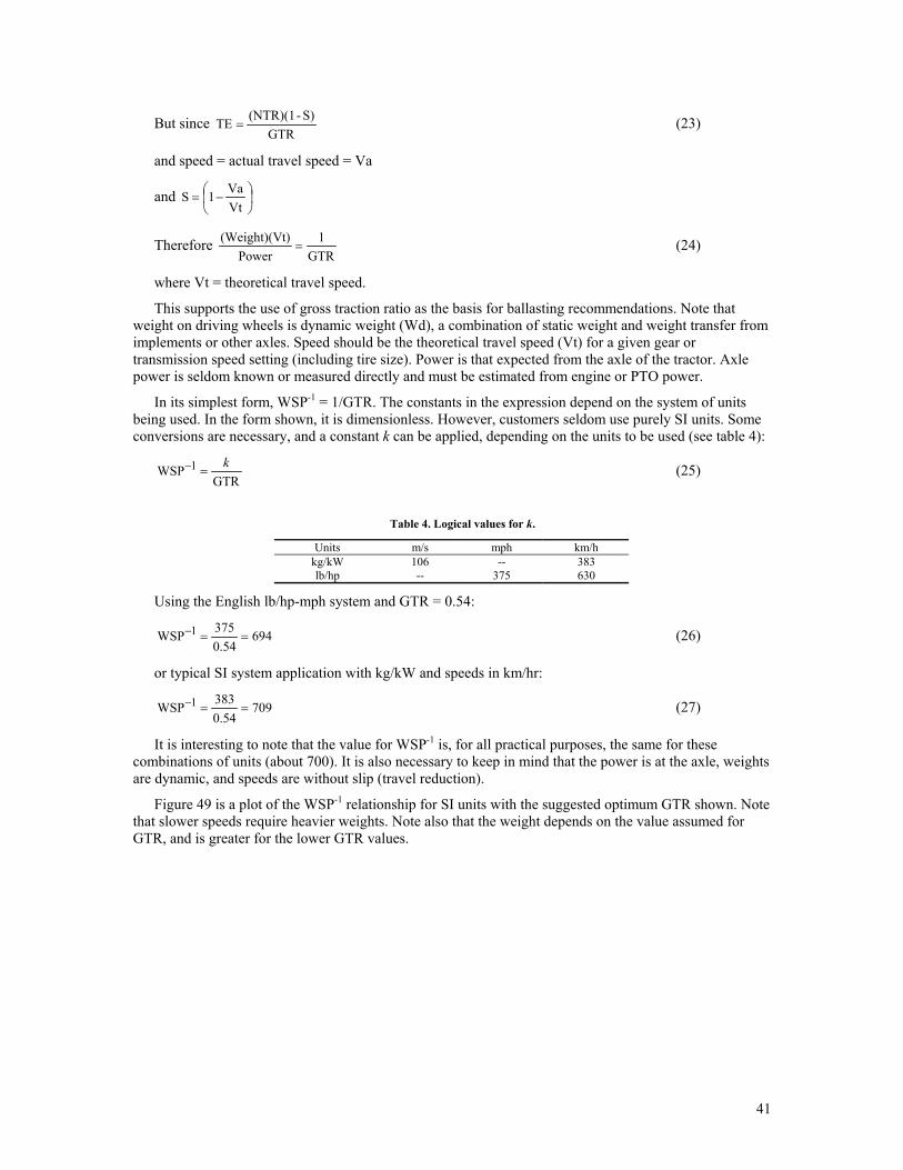
But since GTR

S)-(NTR)(1TE = (23)

and speed = actual travel speed = Va

and

−=VtVa1S

Therefore GTR

1Power

t)(Weight)(V= (24)

where Vt = theoretical travel speed.

This supports the use of gross traction ratio as the basis for ballasting recommendations. Note that weight on driving wheels is dynamic weight (Wd), a combination of static weight and weight transfer from implements or other axles. Speed should be the theoretical travel speed (Vt) for a given gear or transmission speed setting (including tire size). Power is that expected from the axle of the tractor. Axle power is seldom known or measured directly and must be estimated from engine or PTO power.

In its simplest form, WSP-1 = 1/GTR. The constants in the expression depend on the system of units being used. In the form shown, it is dimensionless. However, customers seldom use purely SI units. Some conversions are necessary, and a constant k can be applied, depending on the units to be used (see table 4):

GTRWSP 1 k

=− (25)

Table 4. Logical values for k.

Units m/s mph km/h kg/kW 106 -- 383 lb/hp -- 375 630

Using the English lb/hp-mph system and GTR = 0.54:

6940.54375WSP 1 ==− (26)

or typical SI system application with kg/kW and speeds in km/hr:

7090.54383WSP 1 ==− (27)

It is interesting to note that the value for WSP-1 is, for all practical purposes, the same for these combinations of units (about 700). It is also necessary to keep in mind that the power is at the axle, weights are dynamic, and speeds are without slip (travel reduction).

Figure 49 is a plot of the WSP-1 relationship for SI units with the suggested optimum GTR shown. Note that slower speeds require heavier weights. Note also that the weight depends on the value assumed for GTR, and is greater for the lower GTR values.

41

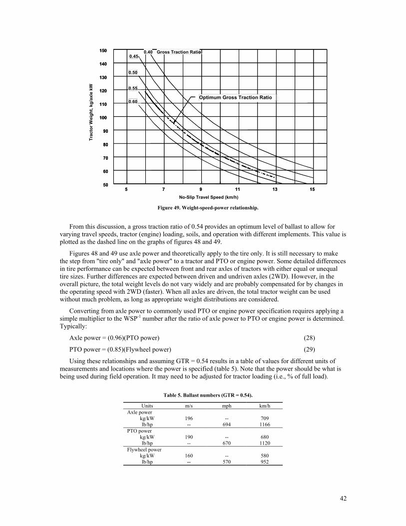
5 7 9 11 13 15 No-Slip Travel Speed (km/h)

150

140

130

120

110

100

90

80

70

60

50

0.55

0.50

0.60

Gross Traction Ratio

Trac

tor W

eigh

t, kg

/axl

e kW

0.40 0.45

5 7 9 11 13 15

150

140

130

120

110

100

90

80

70

60

50

0.55

0.50

0.60

Gross Traction Ratio0.40 0.45

Optimum Gross Traction Ratio

Figure 49. Weight-speed-power relationship.

From this discussion, a gross traction ratio of 0.54 provides an optimum level of ballast to allow for varying travel speeds, tractor (engine) loading, soils, and operation with different implements. This value is plotted as the dashed line on the graphs of figures 48 and 49.

Figures 48 and 49 use axle power and theoretically apply to the tire only. It is still necessary to make the step from "tire only" and "axle power" to a tractor and PTO or engine power. Some detailed differences in tire performance can be expected between front and rear axles of tractors with either equal or unequal tire sizes. Further differences are expected between driven and undriven axles (2WD). However, in the overall picture, the total weight levels do not vary widely and are probably compensated for by changes in the operating speed with 2WD (faster). When all axles are driven, the total tractor weight can be used without much problem, as long as appropriate weight distributions are considered.

Converting from axle power to commonly used PTO or engine power specification requires applying a simple multiplier to the WSP-1 number after the ratio of axle power to PTO or engine power is determined. Typically:

Axle power = (0.96)(PTO power) (28)

PTO power = (0.85)(Flywheel power) (29)

Using these relationships and assuming GTR = 0.54 results in a table of values for different units of measurements and locations where the power is specified (table 5). Note that the power should be what is being used during field operation. It may need to be adjusted for tractor loading (i.e., % of full load).

Table 5. Ballast numbers (GTR = 0.54).

Units m/s mph km/h Axle power

kg/kW 196 -- 709 lb/hp -- 694 1166

PTO power kg/kW 190 -- 680 lb/hp -- 670 1120

Flywheel power kg/kW 160 -- 580 lb/hp -- 570 952

42

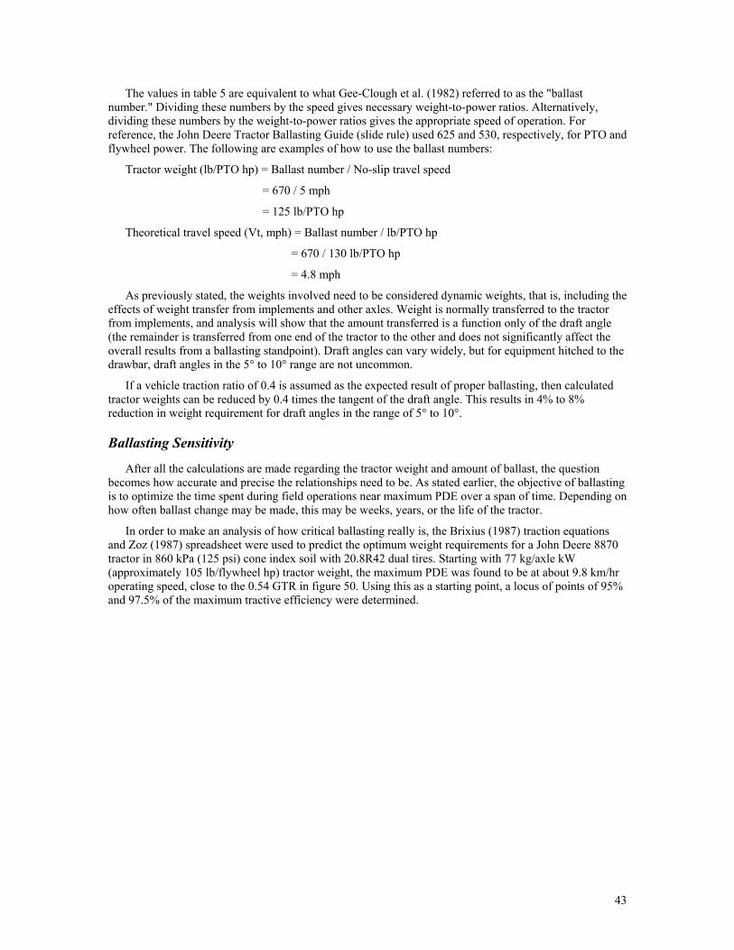
The values in table 5 are equivalent to what Gee-Clough et al. (1982) referred to as the "ballast number." Dividing these numbers by the speed gives necessary weight-to-power ratios. Alternatively, dividing these numbers by the weight-to-power ratios gives the appropriate speed of operation. For reference, the John Deere Tractor Ballasting Guide (slide rule) used 625 and 530, respectively, for PTO and flywheel power. The following are examples of how to use the ballast numbers:

Tractor weight (lb/PTO hp) = Ballast number / No-slip travel speed

= 670 / 5 mph

= 125 lb/PTO hp

Theoretical travel speed (Vt, mph) = Ballast number / lb/PTO hp

= 670 / 130 lb/PTO hp

= 4.8 mph

As previously stated, the weights involved need to be considered dynamic weights, that is, including the effects of weight transfer from implements and other axles. Weight is normally transferred to the tractor from implements, and analysis will show that the amount transferred is a function only of the draft angle (the remainder is transferred from one end of the tractor to the other and does not significantly affect the overall results from a ballasting standpoint). Draft angles can vary widely, but for equipment hitched to the drawbar, draft angles in the 5° to 10° range are not uncommon.

If a vehicle traction ratio of 0.4 is assumed as the expected result of proper ballasting, then calculated tractor weights can be reduced by 0.4 times the tangent of the draft angle. This results in 4% to 8% reduction in weight requirement for draft angles in the range of 5° to 10°.

Ballasting Sensitivity

After all the calculations are made regarding the tractor weight and amount of ballast, the question becomes how accurate and precise the relationships need to be. As stated earlier, the objective of ballasting is to optimize the time spent during field operations near maximum PDE over a span of time. Depending on how often ballast change may be made, this may be weeks, years, or the life of the tractor.

In order to make an analysis of how critical ballasting really is, the Brixius (1987) traction equations and Zoz (1987) spreadsheet were used to predict the optimum weight requirements for a John Deere 8870 tractor in 860 kPa (125 psi) cone index soil with 20.8R42 dual tires. Starting with 77 kg/axle kW (approximately 105 lb/flywheel hp) tractor weight, the maximum PDE was found to be at about 9.8 km/hr operating speed, close to the 0.54 GTR in figure 50. Using this as a starting point, a locus of points of 95% and 97.5% of the maximum tractive efficiency were determined.

43

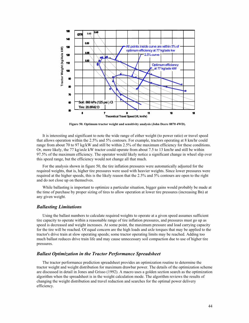
5 7 9 11 13 15

150 140 130 120 110 100

90 80 70 60 50

0.55 0.50

0.60

GTR

5 7 9 11 13 15 Theoretical Travel Speed (Vt, km/hr)

150 140 130 120 110 100

90 80 70 60 50

Trac

tor W

eigh

t (kg

/Axl

e kW

)

0.40 0.45

5 7 9 11 13 15

150 140 130 120 110 100

90 80 70 60 50

0.55 0.50

0.60

GTR

5 7 9 11 13 15

150 140 130 120 110 100

90 80 70 60 50

0.40

All points inside curve are within 5% of optimum efficiency at 77 kg/axle kw

Optimum efficiency at 77 kg/axle kW

2.5% curve

Soil: 860 kPa (125 psi ) CITire: 20.8R42 D

Figure 50. Optimum tractor weight and sensitivity analysis (John Deere 8870 4WD).

It is interesting and significant to note the wide range of either weight (to power ratio) or travel speed that allows operation within the 2.5% and 5% contours. For example, tractors operating at 8 km/hr could range from about 70 to 97 kg/kW and still be within 2.5% of the maximum efficiency for these conditions. Or, more likely, the 77 kg/axle kW tractor could operate from about 7.5 to 13 km/hr and still be within 97.5% of the maximum efficiency. The operator would likely notice a significant change in wheel slip over this speed range, but the efficiency would not change all that much.

For the analysis shown in figure 50, the tire inflation pressures were automatically adjusted for the required weights, that is, higher tire pressures were used with heavier weights. Since lower pressures were required at the higher speeds, this is the likely reason that the 2.5% and 5% contours are open to the right and do not close up on themselves.

While ballasting is important to optimize a particular situation, bigger gains would probably be made at the time of purchase by proper sizing of tires to allow operation at lower tire pressures (increasing Bn) at any given weight.

Ballasting Limitations

Using the ballast numbers to calculate required weights to operate at a given speed assumes sufficient tire capacity to operate within a reasonable range of tire inflation pressures, and pressures must go up as speed is decreased and weight increases. At some point, the maximum pressure and load carrying capacity for the tire will be reached. Of equal concern are the high loads and axle torques that may be applied to the tractor's drive train at slow operating speeds; some tractor operating limits may be reached. Adding too much ballast reduces drive train life and may cause unnecessary soil compaction due to use of higher tire pressures.

Ballast Optimization in the Tractor Performance Spreadsheet

The tractor performance prediction spreadsheet provides an optimization routine to determine the tractor weight and weight distribution for maximum drawbar power. The details of the optimization scheme are discussed in detail in Jones and Grisso (1992). A macro uses a golden section search as the optimization algorithm when the spreadsheet is in the weight calculation mode. The algorithm reviews the results of changing the weight distribution and travel reduction and searches for the optimal power delivery efficiency.

44

9. Conclusions This paper has reviewed traction mechanics and tractive performance parameters to predict the tractor

performance during field operations. By maximizing the tractive advantage of the tractor, more efficient tractor operations can be achieved and the cost of operation can be minimized. The terms for testing tractors and developing predictive equations have be reviewed and implemented into a computer model (spreadsheet) so that operational characteristics can be accessed. Finally, ballast and tire criteria were discussed. It is the hope of the authors that these discussions will provide insights and stimulus into the next revolutionary step in the design and application of traction devices and tractor designs.

Toward that end, several items are noted for future investigation and consideration. The tractive predictions for belted vehicles need to be characterized and built into a computer model with similar ballast and belt operational criteria as has been developed for vehicles with tires. It is also recognized that steering a belted vehicle with a load has certain limitations and that further development is needed. One concept that has merit is the design of an elliptical wheel where the advantages of both of the traction devices (belt and tire) can be embraced. The concept could change the footprint length depending on the operational needs. An elliptical wheel could also make the tire footprint narrower to improve performance and match crop production schemes using narrow rows.

Pressure for the development of new tractor concepts with new roles and tasks will have an impact on field performance. For example, the development of tires and suspensions for high-speed tractors will need to be assessed concerning their impact on field performance. It will be unlikely that the best tires for transport will also be the best for fieldwork. The role of inflation systems and the development of control systems for them have the potential to improve field productivity. The role of a robotic tractor and its performance requirements will need to be developed and assessed. The role of a lighter tractor and concepts to reduce soil compaction are still important.

The assessment of the soil conditions and the enhanced soil's spatial and temporal variations are essential for understanding and predicting tractor operations. The understanding of soil responses from vehicle traffic continues to need practical insights. Traction is attained from a complex interaction of traction devices and soil conditions. Theory, experiment, and field tests have revealed the general nature of this interaction and have provided some insights for analysis of present and future tractions systems. However, plenty is left to investigate and understand before a comprehensive traction mechanics is established.

Acknowledgements

Due to the outstanding contribution to traction and tractor performance made by W. W. Brixius, the authors would like to acknowledge that she changed her name to Christina M. Hollis in April 1992. Dr. Hollis retired from Deere after 29 years in December 2001. Since then, she has continued to be contracted through Deere for various hydraulic, power train, and cooling modeling projects. Presently she owns a company called Omega Consulting, Inc., located near Elizabeth, Illinois.

10. References Al-Hamad, S. A., R. D. Grisso, F. M. Zoz, and K. Von Bargen. 1994. Tractor performance spreadsheet for

radial tires. Computers and Electronics in Agric. 10(1): 45-62.

ASAE Standards. 2001a. EP542. Procedures for using and reporting data obtained with the soil cone penetrometer. St. Joseph, Mich.: ASAE.

_____. 2001b. S296.4. General terminology for traction of agricultural tractors, self-propelled implements, and traction and transport devices. St. Joseph, Mich.: ASAE.

_____. 2001c. S313.3. Soil cone penetrometer. St. Joseph, Mich.: ASAE.

Bloome, P. D., J. D. Summers, A. Khalilian, and D. G. Batchelder. 1983. Ballasting recommendations for two-wheel and four-wheel drive tractors. ASAE Paper No. 831067. St. Joseph, Mich.: ASAE.

45

Brixius, W. W. 1987. Traction prediction equations for bias-ply tires. ASAE Paper No. 871622. St. Joseph, Mich.: ASAE.

Brixius, W. W., and R. D. Wismer. 1978. The role of slip in traction. ASAE Paper No. 781538. St. Joseph, Mich.: ASAE.

Corcoran, P. T., and D. S. Gove. 1985. Understanding the mechanics of track traction. In Proc. Int'l Conference on Soil Dynamics, 4: 664-678. 17-19 June. Auburn, Ala.: Auburn University, Office of Continuing Education.

Dwyer, M. J. 1984. The tractive performance of wheeled vehicles. J. Terramechanics 21(1): 19-34.

Gee-Clough, D., M. McAllister, and G. Pearson. 1982. Ballasting wheeled tractors to achieve maximum power output in frictional-cohesive soils. J. Agric. Eng. Res. 27(1): 1-19.

Jones, D., and R. D. Grisso. 1992. Golden section search as an optimization tool for spreadsheets. Computers and Electronics in Agric. 7(4): 323-335.

Perumpral, J. V. 1987. Cone penetrometer applications – A review. Trans. ASAE 30(4): 939-944.

Shell, L. R., F. M. Zoz, and R. L. Turner. 1997. Field performance of rubber belt and MFWD tractors in Texas soils. In Belt and Tire Traction in Agricultural Vehicles, 65-73. SAE SP-1291. Warrendale, Pa.: Society of Automotive Engineers.

Turner, R. J., L. R. Shell, and F. M. Zoz. 1997. Field performance of rubber belt and MFWD tractors in southern Alberta soils. In Belt and Tire Traction in Agricultural Vehicles, 75-85. SAE SP-1291. Warrendale, Pa.: Society of Automotive Engineers.

Upadhyaya, S. K., W. J. Chancellor, D. Wulfsohn, and J. L. Glancey. 1988. Sources of variability in traction data. J. Terramechanics 25(4): 249-272.

Wismer, R. D., and H. J. Luth. 1972. Off-road traction prediction of wheeled vehicles. ASAE Paper No. 72619. St. Joseph, Mich.: ASAE.

Zoz, F. M. 1987. Predicting tractor field performance (updated). ASAE Paper No. 871623. St. Joseph, Mich.: ASAE.

Zoz, F. M., and W. W. Brixius. 1979. Traction prediction for agricultural tires on concrete. ASAE Paper No. 791046. St. Joseph, Mich.: ASAE.

Zoz, F. M., and R. L. Turner. 1994. Effect of correct pressure on tractive efficiency of radial-ply tires. ASAE Paper No. 941051. St. Joseph, Mich.: ASAE.

Zoz, F. M., R. L. Turner, and L. R. Shell. 2002. Power delivery efficiency: A valid measure of belt and tire tractor performance. Trans. ASAE 45(3): 509-518.

46

traction and tractor performance - asabe technical information library

Documents