UNIQUE OR TYPICAL:

POLITICAL CORRUPTION IN THE

AMERICAN STATES…AND ILLINOIS*

By: Richard Winters

Dartmouth College

September 2012

Paper Originally Presented at the

Ethics and Reform Symposium on Illinois Government

September 27-28, 2012 - Union League Club, Chicago, Illinois

Sponsored by the Paul Simon Public Policy Institute, SIUC, the Joyce Foundation, and

the Union League Club of Chicago

2

Abstract: Thirty-five years of data from the U.S. Department of Justice on “public

integrity” convictions in the U.S. states allows a test of the conventional understandings

of its distribution and causes. Current models of corruption are misspecified, and I turn

to a focus on factors that might affect the “detection” and “commission” of corruption. A

byproduct of such a “theory of corruption” is the “power to predict,” or, in this case,

“postdict” rates of corruption. Given this general model of corruption in the states, it

turns out that Illinois’ corruption rates are almost perfectly predicted -- and at what we

can term a "dull normal" rate. Thus, by theory and by practice, Illinois is not unique. I

conclude with rationales about why the theory may, in the case of Illinois, “mispredict.”

A somewhat different rationale argues that popular Illinois perception of very high

corruption rates may simply misrepresent corruption in Illinois – a case of motivated

reasoning.

*Earlier versions of the paper, co-authored with Amanda Maxwell, were presented at the 2004 meeting of the Midwest Political Science Association; as part of the Morton-Kenney Lecture series at Southern Illinois University, Carbondale; at the 2005 meetings of the American Political Science Association meetings; at the 2006 meetings of the Southern Political Science Association; and at an American Politics Seminar at Dartmouth College. We have profited from comments of Nelson Kasfir, Deborah Brooks, John Carey, Linda Fowler, Michael Herron, and Ronald Weber. Winters thanks members of the Department of Political Science at Southern Illinois University-Carbondale for inviting him to present the initial results of this analysis as part of the Morton-Kenney Lecture Series. The comments of Jason Barabbas, Jennifer Jerit, David Kenney, Frank Klingberg, and Bill Lawrence of SIUC; as well as those of Dick Simpson of UIC, and Lee Radek and Jack Smith of the Public Integrity Section of the U.S. Department of Justice were especially helpful. Winters particularly thanks Professor Jerome Mileur of the Department of Political Science at the University of Massachusetts - Amherst, for his generous support of the Morton-Kenney lectures. Much of this paper is drawn without direct attribution from an earlier set of papers (Maxwell and Winters 2004, 2005, 2006)

3

Unique or Typical: Political Corruption in the American States and Illinois By Richard Winters

I. Introduction: Political corruption may be a personal, “individual” failing of the public servant, a

view that is reinforced by the press with its focus on case-by-case prosecutions.1 In my

“political life” in Illinois politics, that is to say, from the 1950s to the present, five of the

nine elected governors -- William Stratton, Otto Kerner, Jr., Daniel Walker, George

Ryan, and Rod Blagojevich – have been indicted on corruption charges and all but

Stratton convicted. While this is an astonishing rate, is there some more fundamental,

underlying, generalizable meaning to it all?

A more general view suggests that prosecutions for corruption across the states

and across time are peculiarly distributed; not every government – the American states

and Illinois, in particular, in this analysis -- has its “fair share” of corrupt officials.1 Put

directly, an “individualist” understanding is not adequate in explaining public corruption;

simply put, some states are more corrupt than others. If, in fact, the array of corrupt

officials is maldistributed, then specific conditions that vary across the states and across

time may act to heighten or dampen rates of public wrongdoing.2

A third view that I attempt to partially assess here is that some states, such as

Illinois, may have even higher rates than expected of this public “bad” as compared with

other states. As a native Illinoisan and a long-time, albeit distant observer of its state’s

politics, I believe that the popular perception is that Illinois’ politics is uniquely

corrupted.2 It may be that, on average, individuals in Illinois are less honest and,

therefore, more “corruptible” than those in Iowa, North Dakota, or Vermont, and thus the

governments draw from significantly different pools of dishonest individuals for public

service. Or, there may be some more general effects of public employment or

governmental or electoral service in Illinois – and other like states -- that brings out the

latent corruption in public officials. But the empirical question is this: given some

general quantitative measure of “public corruption,” is there some realizable difference

between the observed real rates of Illinois political corruption and that level of corruption

that a general theory would predict? In simple terms, is there an unexplained higher

rate of Illinois corruption, and, thus, the popular perception is accurate.

4

Nothing that I write suggests that corruption is not an issue and an important

problem in American state and local politics. Rather I argue the opposite – it is there, in

every state, but it is “more there” in some states than in others and for perfectly

understandable and generalizable reasons. It just so happens that the “generalizations”

that I advance advantage Illinois and states like Illinois – they are more corrupt than

unlike states, but “unlike” for reasons that we can measure and assess. Put directly,

“for sure, Illinois is corrupt, but it is corrupt just like all other large states, with many

governments, with a heterogeneous population, and where it is difficult, and in some

sense, not worthwhile, for its citizens to exercise greater civic control.” Illinois: meet

New York, Florida, Virginia, and Maryland – you are of a “kind.”

I organize and respond to these views in six more sections to the paper. Section

II defines what I and others mean by corruption in the states and why it is important. I

next review in Section III the recent writings on corruption in the American states. I

focus on what others assume to be the "causal factors" that promote or dampen

corruption. Section IV sets out the operational measures of corruption that I examine

across time and across the states. Section V advances an initial model of corruption, a

particularly powerful statistical model of corruption rates across the states. I also note

how Illinois compares, given this model's predictions, relative to the other states. Part

VI advances a revised model based on suggestions by informed reviewers. I close with

a discussion in VII that suggests reactions to my findings regarding Illinois’ predicted vs.

real rates of corruption and why my findings may be in error. The first is a

measurement issue; the second is an “agency” problem; and the third goes to the heart

of what may be a case of popular perceptual misrepresentation of the real rates of

corruption in Illinois.

II. Corruption in the American States: In a 1960s article, James Q. Wilson writes that political corruption was the

“shame of the American states” (1966).3 Wilson argues that U.S. state governments

are particularly vulnerable to public corruption by comparison with local governments or

the wealthier Federal government. The Federal government has higher levels of

administrative professionalism; Washington draws the best and brightest of

5

administrators alongside more professional and reelection-minded politicians who are

more mindful of the consequences of their and others’ misdeeds. Further, there is

putatively greater review and monitoring of subordinates’ actions by Washington’s

leaders. The links between politicians and bureaucrats may be better “buffered” in

Washington by, for example, oversight Congressional committees which diminish

corruption. Further, national politicians are subject to greater scrutiny by the centralized

and professionalized national press, as well as by large numbers of resident interest

and watchdog groups.

States, according to Wilson, may be uniquely prone to corruption: State

officials may be subject to less voter scrutiny because voters are more poorly

informed about the actions of state officials. Many state capitals are located at some

geographic distance from the states’ larger metropolitan areas, which further

attenuates press coverage of misdeeds. Thus, it may be no accident that state

officials in Springfield, Jefferson City, Tallahassee, and Baton Rouge have national

anecdotal reputations for political corruption.4 State government officials and

bureaucrats handle more discretionary money than their local governmental

counterparts, and, even, conceivably those of the Federal government. One of the

by-products of the development of the modern American federal system of

governance is that an extraordinary amount of money is funneled through state

capitals via the states’ own revenue sources, which is then matched, on many

occasions, by Federal grants and contracts. State officials control, or have a hand in

the distribution of a sizable fraction of public monies spent on governmental purchase

of domestic goods and services. In addition to the sheer amount of intergovernmental

transfers, the bulk of Federal largesse is contributed by out-of-state taxpayers which

may further diminish state officials’ inhibitions in dipping into the state’s public till,

matched, as it is, by out-of-state taxpayers. While J.Q. Wilson’s comment regarding

corruption is most appropriate, “[M]en steal when there is a lot of money lying around

loose and no one in watching” (1966, 31); it is probably even more true when it is

someone else’s money.

Wilson argues that local governments are vulnerable, but less so than state

governments. Put simply, there is less to misappropriate, and typically local officials

6

are more likely to be subject to closer scrutiny by local press and voters. The New

England experience suggests that there may be greater scrutiny of officials’ actions by

local voters in local elections, and that scrutiny is heightened as the size of local

government shrinks (detection of corruption is easier) and the population becomes more

homogeneous.5 Self-aggrandizing displays of personal largesse financed by local

corruption may be obvious to local citizens. Bryan (2004), Wilson (1961) and Winters

(2008) argue that local voters more closely monitor local politicians, because local

politicians’ actions directly affect local tax rates.

The meanings of corruption: Corruption for our purposes is an official’s

concealed private misappropriation of a public right for gain to self (see also Nye 1967,

Rose-Ackerman 1975, Shleifer and Vishney 1993, Treisman 2000, Gordon 2009). 6

Gunnar Myrdal (1968) unpacked the proximate links between public officials and

corruption: there is high value associated with officials’ control over the power to

positively or negatively coerce individuals.7 State-issued licenses are required to

positively perform certain acts. State permits are necessary in order to engage in many

transactions and state-issued grants of money support and advance local projects.

Further, while I ordinarily view a corrupt act as a “positive” one – the public official has

to do “something for someone” in order to obtain the illegal rewards, there is also the

power to do nothing, to overlook violations or regulations. In this case, individuals bribe

officials for governmental inaction. Myrdal argues that bureaucratic and political control

over valuable rights, “adds greatly to the incentives for, and the rewards of graft and

corruption.” Governmental control over the “rights to coerce positively and negatively”

constitutes the resource base for corruption.8

A perverse effect of corruption is tax costs. Corruption is a non-statutory tax on

citizens by “upping the costs” of public activity, a public cost-increase that has not been

formally approved by governmental action. Further, as Shleifer and Vishney (1993)

note, the “imperative of secrecy makes bribery more distortionary than taxes” (600,

italics in the original). Cross-nationally, corruption appears to dampen economic

activity, not only for reasons of corruption acting as if it were a further monetary “tax” on

action, but also for reasons that corruption encumbers dealings with heightened

transaction costs and the complicated ambiguities of the means to enforce a corrupt

7

bargain (Mauro 1995; Ades and di Tella 1999; Treisman 2000). Corruption in the states

may also result in dampened growth in income, employment and median home prices

(but, see Glaeser and Saks 2004).9 Corruption exacts non-monetary costs as informal

transactions multiply. Further, while Hibbing and Theiss-Morse (1995, 2000) conclude

that the American public accepts the outcomes of politicians’ actions, nevertheless

citizens have profound doubts about the process of getting to those actions. It is not a

great leap of inference to argue that some part of Americans’ anxieties about the quality

of the political process revolves around uncertainties about whether and who paid

whom, how often, how much, and when, in order to get something done, undone, . . . or

not done.

III. The Political Analysis of Corruption: Studies typically focus on the likely causes of corruption such as the impact of

judicial resources; whether poverty or economic growth fosters corruption, or whether

cultural factors such as other crime rates affect corruption propensities (Meier and

Holbrooke 1992, Schlesinger and Meier 2002). Traditional political factors of “size of

government, bureaucracy and rent-seeking” and the impact of party and electoral

competition (Hill 2003) also may lead to corruption variations for reasons of varying

political “observability, transparency, and trust” (Alt and Lassen 2003, 342).

In an early study, Welch and Peters (1978a, b) surveyed several hundred state

senators in twenty-four American states, asking legislators how best to measure

corruption, and concluded by asking about their perceptions of corruption in their

state.10 Weak findings existed for lower tolerance for corruption among women

legislators, among freshman members, liberals, and urban legislators. The industrial

East, Midwestern, and Southern states had higher perceived corruption, while states in

the mountain, prairie, and New England regions were lower.11

Michael Johnson (1983) and David Nice (1983) first analyzed the data from the

Public Integrity Section of the Department of Justice on annual convictions for

corruption.12 Johnson (1983) examined early data from reports from all 85 substate

U.S. districts (the courts of original jurisdiction) and discovered that the underlying

district political cultures and states’ level of political participation affect corruption

8

conviction rates. Nice (1983) also found that the predominant “moralistic” political

culture and education levels in states dampened corruption rates.

Meier and Holbrook (1992) conducted the most wide-ranging examination of the

causes of corruption convictions from 1977-1986, marshaling twenty-two variables

analyzed in clusters of judicial resources, historical/cultural, electoral/political, and

bureaucratic/structural. They winnowed the list to eight variables that appeared best

related to convictions, and of these, gambling arrests, government employment, and

percent urban were positively related, while factors of percent college graduates and

interparty competition were negatively related.13 The authors were not entirely satisfied

with their own analysis and in a subsequent study, Schlesinger and Meier (2002),

reexamined the variables using 1986-1995 DoJ data and discovered few persistent

causal factors. However, a factor analysis discovered three significant underlying state-

by-state traits, which they labeled “cosmopolitan” states (with more prosecutions),

“traditionalist” states (also more prosecutions) and states with “low social capital” (also

more).

In an earlier paper, Maxwell and Winters (2004) took Meier and Holbrooke’s

analysis one step further and reexamined four of their models, fifteen variables in all,

for the next panel of U.S. DoJ corruption data, the 1987-2000 data set, the data set

also further analyzed in this article. Cluster by cluster, the only variables that

consistently accounted for prosecution variation in 1977-86 period and also in the

1987-2000 period were percent urban, percent college graduates, voter turnout, and

gambling arrests. When pitted identical final sets of variables for the two period data

sets (those in Table 6 of the Meier and Holbrook paper), the only consistent predictor

was the negative impact of voter turnout on statewide corruption convictions.

Hill’s analysis (2003) is consistent with this political/electoral understanding of

the causes of corruption convictions. He focused on measures of interparty

competition in the states which should “increase the likelihood of the exposure of or

punishment for corrupt acts,” in our conceptualization, the “detection” of corruption

(613). Hill employed Meier and Holbrook’s 1977-1987 conviction measure and found

that a measure of democratization that is a composite of party competition and

9

electoral turnout rates is negatively related to convictions, while controlling for other

important factors such as government size, urbanism, and median income.

Adsera, Boix, and Payne (2003) confirmed a socio-political understanding of the

causes of corruption. In their analysis of cross-national, as well as cross-American-

states data, rates of public malfeasance are diminished by regular, free elections and by

how well informed voters are about political choices. The credible threat of the loss of

power via the electoral process disciplines honesty among officials, which is further

reinforced by the belief that well-informed voters more closely monitor officials’

behaviors. In the American states, they examine the same dependent variable that I

employ here and conclude that “. . . having reliable and efficient politicians derives from

the presence of politically active, well-informed, sophisticated electorates” (480).

Cross-nationally, Mauro (1993) as well as LaPorta, et al. (1999) claim that ethnic

fractionalization, heterogeneity, or, as I put it in this examination, social diversity, also

positively affect rates of corruption. Glaeser and Saks (2004) examined the states and

concluded, consistent with Adsera et al., that their results “…are remarkably similar to

those at the country level” (p.3). Higher levels of income and education dampen

corruption rates, while racial heterogeneity is positively, albeit more weakly, related.14

IV. The Measure of Political Corruption: From 1976 to 2010, the Public Integrity Section of the U.S. Department of Justice

presented the numbers convicted in 27,938 corruption cases across the 50 states. The

barely readable Table 1 arrays the DoJ numbers of convictions by state year.

10

11

Table 2 arrays this data in summary and more readable form.

Column 2 presents the total number of such convictions over the thirty-four year

period, and in this array, Illinois is the third ranked state. Of course Illinois is the fifth-

12

most well-populated state, so we would expect a high ranking simply on the basis of

demographics, but which demographic? Population has been used by one set of

analysts (Glaeser and Saks 2004) as a weighting variable, i.e. “number of convictions

per 1000 state population,” but the convention in political science is to control for the

relevant demographic eligible for corruption indictments and convictions, and the most

frequently used such variable is the “number of federal, state, and local elected officials

in the state” (Meier and Holbrook 1992, Meier and Schlesinger 2002, Adsera and

colleagues 2003, Hill 2003, Maxwell and Winters 2003, 2004, 2005, 2006). Column 4 of

Table 2 ranks the American states by such a number and note that Illinois has, about

25% more elected officials than the next state, Pennsylvania, and, therefore, has the

largest number in the “eligible” pool of “public officials.” Hawaii is the opposing outlier,

averaging about 180 officials per year.15 Next lowest in officialdom are Delaware and

Rhode Island with 1100 officials. If we, as others have, divide the number of convictions

by the number of officials -- the plausible "target group" for corruption accusations -- we

get an ordering of states with Florida at the top of the heap and Vermont at the bottom,

as our variable of interest in column (6) of Table 2 – the number of convictions by state

as a fraction per 1,000 elected public officials. Note that Illinois has now tumbled to the

middle of the distribution – a finding that will be repeated in all of my subsequent

analyses.

Do the DoJ numbers adjusted for judicial domain appear to be a reasonable

proxy for “real corruption?” Put differently, how would we know that we are adequately

measuring a real trait of public corruption? Corruption, if the Department of Justice

data is a good proxy for the de facto statewide trait, does not distribute itself in obvious

ways.16 The typical state averaged about 15 prosecutions per year, but this ranged

from 1 per year in Vermont to nearly 115 per year in New York. As this suggests, the

conviction rates vary by size of state; highly populated states and states with many

governments have many more cases of corruption. At the limit, over the quarter

century, New York has recorded 2500 such convictions, while Vermont trails with a

scarcely appreciable thirty-one.

There does appear to be some face validity to the five most corrupt states in

convictions per number of elected officials: Florida, Virginia, Maryland, Louisiana, and

13

California. Perhaps the list of the five “least corrupt” makes even more intuitive

sense: Vermont last, then Nebraska, New Hampshire, North Dakota, and Iowa. The

number of convictions per thousand officials is strongly curvilinear, and I adopt the

formulation for my regression analysis used by others in the literature (Meier and

Holbrook 1992, Schlesinger and Meier 2002, Adsera and colleagues 2003, and Hill

2003) that the most appropriate measure of Justice Department indicated public

corruption is the log of the number of convictions per 1,000 elected officials in a state.

Illinois should appear, by conventional wisdom, high on the list, but, in fact,

ranks 25th. But the median figure for Illinois may mask a more profound regularity.

Illinois has 30% more elected officials than the 2nd ranking state, Pennsylvania.

While political corruption should be linked positively to the number of officials, very

large numbers of officials may veil public malefactors. Thus, the middling numbers of

the Illinois convictions may imperfectly reflect an underlying higher real rate of

undetected corruption. This may be due to an exhaustion factor at the Federal

Attorneys’ offices in Illinois as the numbers of potential malefactors increase with the

number of officials. Many acts of official corruption in Illinois may be too trivial for

federal judicial action. 17 Nevertheless, we expect corruption convictions per 1000

officials to fall with rising numbers of governments, but to fall with diminishing

decrements. Our model, discussed below, accounts for this by using the number of

governments and the number of governments squared as independent variables in

explaining corruption per numbers of elected officials.18

Maxwell and Winters (2004, 2006) further test for internal validity by the

consistency of the measure. Meier and Holbrook (1992) examined the data using

years 1977 to 1986. The simple correlation between their and our measure (for the

1987-2006 period) is +.85. If we average the convictions per 1000 officials for the six

5-year periods from 1976 to 2005, the inter-period correlations average +.66.

However, the correlations average +.89 for the four periods from 1985 to 2005

indicating that after an initial set of years, an equilibrium figure of prosecutions per

year by state appears to become established. Further, corruption convictions over

time in states appear to be relatively stable processes. For 30 of the 50 states, the

simple average figures for each state for the time period appear to be the best

14

guesstimate.19 No states show a decrease in convictions over the two-plus decades.

States that have the steepest rates of increase are Florida, Missouri, California,

Washington, Ohio, and Texas.20 A handful of small states show great relative

increases – an increase of 2 cases per year in Wyoming and Idaho and with North

Dakota and Washington increasing between 1 and 2 cases per year. 21

V. A Model: I argue that the determinants of corruption follow from the likelihood of its

“commission” and “detection” (Becker 1968). I propose an initial model (Model I) that

focuses on seven indicators of four across-state traits that shape the likelihood of the

commission of corrupt acts and their likely detection. I then add, in Model II, two new

factors as suggested by informed reviewers.

15

(1) A “commission” factor: The “greater the size of state population” the

greater the corruption. As size increases, the public treasury will appear to the

corruptible official to be more and more a common pool into which officials can dip

with barely observable consequences, and, thus, appearing to hurt no one. If so, we

suspect that there may be an opposing effect, that “smaller states” will have markedly

lower levels of corruption. In small states, corruption may pose such a perceived

threat to the “idea” of the “state” as an idealized, comprehensible “commonwealth of

all” that the power of the idea serves to deter officials. Those in small states may well

understand their position as being in the employ of the commonwealth of all, and thus

have higher internalized norms of self-restraint. To steal from another in the smaller

“all” is, in effect, to steal from those who live right next door, or the next town over. If

so, I expect a positive sign for the variable of the size of population and a negative

sign for the squared term indicating the sharply lower levels found among states with

small populations. The confirmatory scatter plot of population size and the log of

corruption convictions appear in Figure 3 along with a curve that best approximates

its quadratic fit.22

16

(2) I pursue a parallel line of argument and resurrect a form of J.Q. Wilson’s

original observation about the ethnic makeup of a state, and suggest another

“commission” factor. States with high levels of “demographic population diversity” will

have correspondingly high levels of corruption.23 As diversity in the states increase,

contributions via taxes to the public treasury are collected from a variety of

constituencies – ethnic ones in our conception.24 Corrupt officials can rationalize

dipping into the public coffers by arguing that they are primarily skimming from unknown

others – and likely very much unlike themselves.25 Diversity rationalizes corruption as

extraction from others unlike the self.26 Graphic and regression diagnostics suggest that

this is a simple linear relationship – as the heterogeneities of states’ populations grow,

as ethnic groups become more discrete and less like one another, corruption rises.

(3) Corruption rates should vary negatively with “numbers of ‘corruptible’

governmental bodies” – falling as the numbers of governments in states rise. Stated

at the limit, states with few governmental bodies are likely to have high rates of

corruption prosecutions per 1000 elected officials.27 The relationship, I believe, will be

non-linear. States that have particularly large numbers of governments, Illinois and

17

Pennsylvania, for example, will have fewer convictions, but more than states with

modest numbers of governments. Thus we expect a negative sign from the linear

term and a positive sign from the squared term reflecting the distribution of values at

the tails. Why so? In the case of the DoJ measure, I do not believe that the US

Department of Justice distributes its attorneys for cases on “public integrity” to the

states based on numbers of governments; rather, they are probably distributed as a

function of the general caseload. If so, Minnesota with its 3500 governments, thus,

many “elected officials,” will probably have a number of US Attorneys overseeing

public integrity cases roughly equal to states of similar population size, such as North

Carolina and Florida, but each with about 1000 governments – 30% of the number of

Minnesota governments.28

The potential caseload of possible corruption may be many times higher in

Minnesota due simply to the larger numbers of governments with their elected

officials. We would expect, however, that Minnesota with its many more governments

will have fewer corruption convictions when stated, as we and others do, as

proportional to the number of officials. There may be a legal behavioral explanation,

as well. As the number of governments increases, the likely scale of corruption – the

gains from the corrupt act -- becomes smaller, and thus of less interest to the

prosecutorial ambitions of energetic U. S. Attorneys.

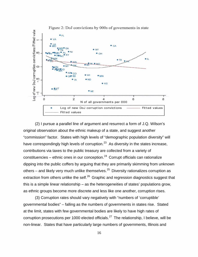
The distribution of our DoJ corruption measure by the number of governmental

units appears in Figure 2 along with the linear and quadratic fits of the underlying

distribution. Note the linear relationship is predictably negative – as the number of

possible corruption locales increase, as measured along the horizontal axis,

conviction rates fall. However that masks a relationship of a rising rate as the US DoJ

confronts the reality of politics in Illinois, Texas, and Pennsylvania. A simple model

predicting the corruption rates with the variable of “number of all governments in the

state” and its “square” yields the expected negative for the linear term and positive for

the quadratic.29

18

(4) Finally, states with “civic-minded, well-informed political cultures,” as

measured by high percentages of college graduates and a Census Bureau-derived

measure of high levels of individual-level civic involvement, will have lower rates of

corruption for reasons of “detection.”30 Well-educated citizens, I argue, are less

tolerant of corruption. Well-educated citizens are better informed and more likely to

wreak electoral vengeance on public malefactors and their sponsors/colleagues.

High levels of civic involvement may also lead to closer ties between citizens and

officials and likely constrain officials to be more open and transparent in their dealings

with the public.30

My expectation is that this seven variable, “four-concept” model will account for

substantial variation in the log of the 1987-2000 sum of DoJ convictions per 1,000

elected officials, I also report on a time-series, cross-sectional, fixed effects (for time)

19

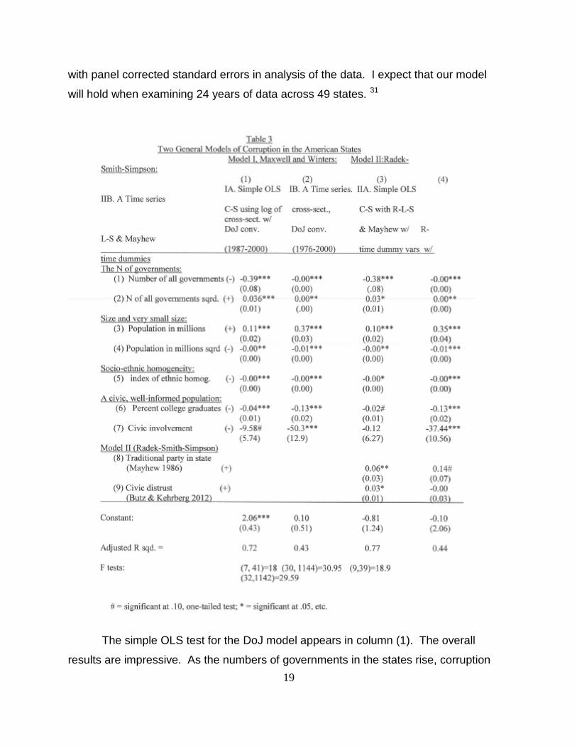
with panel corrected standard errors in analysis of the data. I expect that our model

will hold when examining 24 years of data across 49 states. 31

The simple OLS test for the DoJ model appears in column (1). The overall

results are impressive. As the numbers of governments in the states rise, corruption

20

convictions fall. I explain this with reference to scarce Department of Justice

resources that must be spread over a larger number of possible corruption sites in

states with large number of governments. Alternatively, as the numbers of

governments grow in these states, the possible benefits of corruption fall, so there

may be less incentive for dipping into the public till. Alternatively, large numbers of

governments necessarily draw out large numbers of amateur and part-time officials –

both elected and unelected – with an unknown consequence, but conjecturally

positive, on the probability of corruption. The size and significance of the coefficients,

negative in the linear term and positive in the squared term, indicate this curvilinear

effect. States with small numbers of governments have higher appreciable corruption

conviction rates per 1000 elected officials, and the rate of convictions falls among

those with larger numbers, but at a declining rate. As Figure 2 suggests, it begins to

rise again with particularly large numbers of governments as corruptible bodies. The

coefficients for these two measures are significant in both the simple OLS test and in

the unreported results of an analysis with robust standard errors.

I further hypothesized that the population size of the states would have non-

obvious effects. Officials in states with large populations might be more tempted to

corruption given the anonymity of their position in a large, multi-division, multi-level

organization and, thus, the appearance of the diminished impact of their personal

corruption on the state. Officials in very small states may have a greater sense of the

proximity of their own corrupt activities on the public treasury and the negative impact

on the public interest of their extra-legal activity. We also believe that a corollary trait is

that officials in small states may have a heightened sense of being engaged in common

activities that gives meaning to the notion of the commonwealth of all, and that sense

may decline with rising population. If true, we expect a positive sign for the simple

population variable and a negative coefficient for the quadratic, squared, term. In the

OLS test, both coefficients are sizable and in the predicted positive and negative

directions, and each is significant in the unreported robust regression estimates, as well.

I also argue that the likelihood of corruption rises in American states as the

states’ populations become more diverse. The proxy measure for the more general

trait of social “diversity” is a nine-element Herfindahl index of ethnic homogeneity.

21

The results of the OLS regression argue that as the states’ ethnic homogeneity

rises, corruption rates fall. We believe that this is a particularly robust finding. This

highly positive relationship holds when calculated with either the Black or Hispanic

percentages of the states’ populations excluded and the Herfindahl index

recalculated, and when both are excluded. The relationships hold, as well, in a

regression that includes the variables of percentage Black in the population and the

percentage Hispanic in the population along with a now-seven-element Herfindahl

index. Further, the seven-element homogeneity index is significant and in the correct

direction, while neither the Black nor Hispanic variables are significant. I argue that

no single ethnic element of an index of homo/heterogeneity accounts for corruption

rates. A very strong case can be made for the impact, not of any particular ethnic

group’s impact on heightened corruption, but instead the combined effect of diversity.

States that have many population components appear to have greater corruption

rates, irrespective of the identity of the array of ethnic groups that comprise the

population.32 The explanation for this is simple: in a state with a heterogeneous

population any single official will perceive his or her act of malfeasance as largely

affecting a population that is unlike the self. Diversity diminishes officials’ moral

constraints that might limit exploitation of the commonwealth. In diverse states, the

population appears less “common” to the corrupt official.33

Finally, I argue, as do others before us (Hill 2003, Alt and Lassen 2003,

Adsera, Boix and Payne 2003), that a participant, well-informed population should

lead to public honesty. This is measured by (1) via the percent of the states’

populations that are college graduates and (2) by a direct measure of the proportion

of the states’ populations that claim to have volunteered in some kind of civic

activities. In the simple OLS model the education variable is a strong predictor of

corruption rates, while the civic involvement variable is weaker, albeit significant at .10

level.34 In an unreported robust regression, both factors are strongly related to

corruption in the predicted direction – falling as the educated fraction of the electorate

rises and falling as the rates of popular civic involvement rise. In the simple OLS

model and its robust equivalent, our seven variable model accounts for 72% of the

variance in the dependent variable.

22

The Department of Justice data on convictions is available on an annual basis

from 1976 to 2000, so a time-series cross-sectional (TSCS) design is feasible.

Further, state population figures and, thus their squares, are available annually. The

numbers of governments and the squares, as well as college degrees as percent of

the population are available only on the decennial census years. For these variables,

we began with the 1970 Census data and interpolated the annual figures between

1977 and 1980. Beginning with 1981, we used the same interpolation method to

generate annual figures for this decade, and we followed a similar methodology for

the years between 1990 and 2000. A truncated measure of ethnic homogeneity is

also available on a decennial basis, reliably so for Black, Asian American, Hispanic,

and “other.” Our measure of “civic involvement,” however, is available only for the

1990 period. Our solution was to generate a TSCS data set of annual data from

1977-2000 for the log of the convictions rate per 1000 officials and for the state

population figures and the squares. We added the annually-interpolated data on

governments, college degrees and a Herfindahl diversity measure based on the

above-mentioned four ethnic population components for the years between decennial

censuses of 1970, 1980, 1990 and 2000.

Our civic involvement measure was entered identically for each state for each

of the twenty-four years. We also added, per convention, dummy variables for each

time period less one. State-by-state fixed effect variables could not be added

because of the invariance over time of our civic involvement variable. We employed a

Prais-Winsten regression with panel corrected standard errors with an assumption of

a first order autocorrelation.35 Our results appear in column II of the table and are

supportive of our original model: States with large populations have more corruption;

states with small populations much less. States with smaller numbers of government

have more corruption, but states with particularly large numbers have proportionally

greater. And corruption as a dynamic process is lower in states with civically involved

populations, those with well-educated populations and in states that are ethnically

homogeneous.

23

VI. A Revised Model: The discussion above was reviewed by three individuals who bring special

purchase to the topic of political corruption in the American states: Lee Radek, the

former head of the Public Integrity Section of the US Department of Justice; Jack Smith,

the present head of PIN; and fellow-panelist Dick Simpson, a former Chicago City

Councilmember and a longtime observer of Chicago and Illinois politics. Each argued

the identical case for adding two “omitted variables”: (1) a measure of traditional party

organization in the states, one more likely organized by “material benefits,” or “machine-

type politics,” and (2) a measure of citizen distrust. Reasonably good measures of each

are now available to scholars of state politics. David Mayhew’s Placing parties in

American politics (1986) sets out a measure of “traditional party organization” (TPO) an

across-state analysis where the highest scores ( = 4 and 5) are reserved for what he

terms “organization states,” where political parties have substantial autonomy, parties

are long-lasting, largely hierarchical in nature, exercise control over nominations to a

wide number of offices, and the parties traditionally rely more on “material” rather than

“purposive” incentives to motivate party workers (Mayhew 1986,19-20).36 This last trait

suggests equivalence to what we normally think of as “machine politics,” and Mayhew

notes the link (p. 21) but restricts his use of this term to TPOs at the local level, e.g.

Cook County. But for our purposes, Mayhew scales the fifty states beginning for the

late 1960s time period on a 5 to 1 scale indicating how closely the state’s two parties

adhere to the norms of a “traditional party organization” (the scaling results appear in

Table 7.1, p. 196 of Mayhew 1986). After trying any number of formulations, the most

powerful measure appears to be Mayhew’s original 5 to 1 scoring system. Thus, I

expect that the more “traditional” the form of party organization, the greater the rate of

corruption convictions.

A new manuscript by Butz and Kehrberg (2012) exploits the computer technique

of “multi-level regression and post-stratification” to estimate state-by-state levels of

“social mistrust.” The authors used the ANES question of “Generally speaking, would

you say that most people can be trusted, or that you can’t be too careful in dealing with

people” to estimate state-by-state levels of “distrust.” I expect, of course, that high

levels of average distrust among citizens will be associated with higher rates of political

24

corruption convictions. I note at the outset that there is an endogeneity problem at work

here: high levels of social distrust may be a cause or an effect (or both) of high levels of

corruption among public officials. For our purposes, however, this is not a serious

issue; we are simply trying to generate a powerful statistical model and predicting the

levels of corruption with the expectation that Illinois will have a high positive residual.

Therefore, high levels of social distrust will be associated with high levels of political

corruption. The revised visual model appears in Figure 4.

25

Columns (3) and (4) of Table 3 display the regression results – both for our

averaged 1987-2000 values of corruption convictions as a “cross-sectional estimate,”

and exploiting the data over time as a time-series/cross-sectional model. In both

26

estimates, the estimates in our original model remain powerful and significant, except

for our two estimates measuring “a civic well-informed population.” With the added

variables, both of the regression estimates for “percent college graduates” and “civic

involvement” are attenuated with the latter particularly affected. However, in the

averaged 1987-2000 cross-sectional estimates, the “traditional party in the states”

and the “civic distrust” variables are important factors in accounting for corruption.

And, while the added estimates for “party organization” and for “social distrust” are

useful variables in the cross-sectional model, both are severely attenuated in the

TS/CS model, while the two measures for a “civic, well-informed population” regain

their importance.

VII. Discussion and Conclusion: The question of particular interest at this point is, “OK, so how does Illinois fare

in these analyses?” I left the discussion at page 7 and 8 noting that, while Illinois had

the third largest number of corruption convictions for the period, once you “control” for

the plausible pool of possible prosecutorial “targets,” the state falls to the middle of

the pack – at 25th of the 49 states in our analysis. Table 4 presents the rank order of

residuals on the “log of convictions per 000 elected officials” for the 1987 to 2000

period in column (1), and again the state falls squarely at the “very well explained”

mark at the midpoint of the ranked states. Some states, such as NH, MA, AR, and VT

have much lower rates of convictions given our explanatory model, while VA, MD,

WA, MO, and MN have higher than expected rates. But Illinois’ expected rate of

prosecution convictions is well-explained by the model. Column (2) gives the rank

order for the cross-sectional data for the full nine-variable, Radek-Smith-Simpson

model, and I find the same results. A similar result occurs if I average the residuals

by state over the span of the TCCS model, as well for each of the two models as

represented in columns (3) and (4). The conclusion of the data analysis is

inescapable: if you employ the available data on corruption in the American states;

weight the data in the conventional manner; account for its variation across the states

and across time, Illinois is not uniquely corrupted. In fact, it is quite ordinary. Why?

27

[

It strikes me that there are a number of explanations for this unexpected

outcome: the first is the “weighting problem” as it affects Illinois; the second is an

agency/agenda explanation, the third is a “number of governments/public officials

28

explanation, and the fourth is that there is a systematic popular misperception of

actual corruption in Illinois – or, stated somewhat differently, a case of widespread,

popular “motivated reasoning,” that is to say, Illinois citizens are convinced that their

state is more corrupt than others, and there is no way that the simple facts (or even

the complex facts) of the case can convince them otherwise. “My mind is made up;

don’t confuse me with the facts!”

1) Illinois has 25% more elected federal, state, and local officials as compared

with the next-ranking state and about four times more than the typical state. Had Illinois

the same number of officials as the typical state – about 8,000 – it would have remained

at the top of the heap of “convictions per 1000 officials” at fourth rank exceeded only by

Florida, Virginia, and Maryland. Illinois high ranking in the “raw count” and its middling

ranking in the “weighted by officials” account may simply reflect the fact that there is a

limit to the number of corruption cases that one U.S. Attorney and office – or in Illinois’

case, three such offices37 -- can bring in a judicial district. One crude test for this is the

following: arbitrarily reassign Illinois’ “officialdom down from 38,000 elected officials to

the states’ mean of 8,000 with the new number in the “convictions per 1000 officials and

re-run the regressions. Illinois is now third-ranked state in the “number of convictions

per 000 officials” (now 8,000), but in the regressions, Illinois’ residual again lapses to

the middle of the pack – perfectly well-predicted by my model. While this is a crude

“what if…” test, nevertheless it suggests that what is going on here is that nothing out of

the ordinary characterizes Illinois corruption conviction rates.

2) With 25% more governments and elected officials than the next largest (in

PA), a somewhat different way of casting the “number of officials/governments” issue

argues that the very large numbers of each militate against an adequate judicial

treatment regarding corruption in Illinois, while supporting the cynical public views that

there are lots of officials out there getting away with being “on the take.” As you multiply

the number of governments, you multiply the number of opportunities for corruption; and

while you may diminish the “personal take” of each corrupt act of each official as

government “domains” shrink; you multiply the burdens on the judicial process for

coping with corruption; thereby likely leading to increasing the costs of voters to fully

inform themselves and electorally control corrupt governments/politicians. More

29

governments ineluctably lead to both the actuality as well as the perception of

corruption.

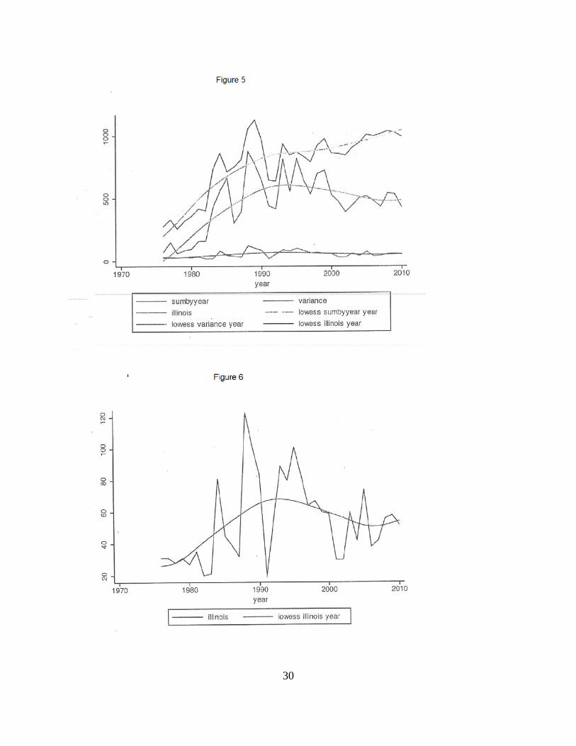
3) Figure 5 and 6 suggests these limits. The figure arrays graphically by year

the total number of PIN prosecution convictions by year (in the top line), the variance

of the annual state-by-state data across time (the bottom line). The variance is the

square of the standard deviation of the annual state-by-state data. The curved lines

for each of the three lines represent the “lowess” trend in the change over time in the

data. The “sum by year” variable – the top line – represents the total number of PIN

convictions by year. It indicates a relatively steep ascent from 1976 to about 1990

and then a more gradual, “evening-out” period from about 1990 to 2000, and a

slower, albeit gradual rise since. This should not be surprising. The section was first

organized in 1976 and became a dedicated, line-item part of the DoJ criminal division

in 1978. Like every new agency, workload growth increased rapidly at the outset, but

soon began to slow and even-out as the agency faced budgetary and personnel

limits. Growth cannot go on forever, even though corruption may be absolutely

increasing year-by-year. The budgets and personnel at the departmental level (DoJ),

divisional (Criminal Division), and section (PIN) have real finite limits. What is true for

the section must, as well, be true for each judicial district. And even though Illinois is

graced by three judicial districts, there are limits to how much attention can and

should be paid to corruption. The three Illinois Offices of the US Attorneys have

crowded agendas and each added corruption case taken on at some point

necessarily crowds some other criminal case off that office’s agenda of cases. The

variance line and its lowess estimates indicate that there has been a gradual

“evening-out” of the distribution by states is slowly becoming more like one another in

this PIN cases by year.

30

31

The lines in Figure 6 array the year-by-year numbers of PIN cases in the three

Illinois judicial districts along with the lowess line. They suggest that an equilibrium

level of convictions at the aggregate level was reached about 1990. While there are

substantial year to year changes in Illinois convictions numbers, the lowess line

indicates the sharp rise in the data at the outset, and then an evening-out process

where corruption cases begin to reach “limits.” Mimicking the overall figure, there

does appear to be a small rise in the last few years. All of this indicates to me a

gradual rise with both a routinization of corruption prosecutions in a large organization

(PIN) and in three of its component parts – Illinois’ Northern, Central, and Southern

District Courts, but also the suggestion of an agency limit. The offices of the U.S.

Attorneys must balance the demands for staff to prosecute corruption cases with the

demands for prosecuting all other kinds of criminal cases. They cannot be all things

to all people.

4) My conclusions about the ordinariness of corruption in Illinois does not

square, I suspect, with popular understandings of Illinois politics, and I suspect that it

does not square with the opinions of the organizers of this conference. We are

meeting in Chicago at a conference sponsored by a well-established and well-

regarded academic public policy institute and assisted in its financing by a well-known

and politically-significant charitable foundation. The ordinariness of Illinois certainly

does not square with the judgments of those who were reputed to be experts. Boylan

and Long (2003) surveyed (early in 2000s) journalists nationwide about political

corruption in their state and Illinois ranked third highest in journalists’ opinions among

the forty-five states with usable numbers of returns. And, I suspect, if one were to

quiz Americans around the country about political corruption at their local and state

environs, Illinois citizens might well top the list of critical, cynical, and distrustful

citizens and voters. Can I square the indications of politically corrupt uniqueness –

Illinois as a limiting case – with my results?

If, as the Turkish aphorism claims, “a fish rots from its head,” then the penal

record of Illinois governors – four of the last nine in the pokey and five of nine indicted --

may indicate to Illinois’ citizens that there is an underlying, fundamental malignancy that

afflicts politics in Illinois generally. “If five of nine governors are guilty as charged, isn’t

32

this just an indicator of a fundamental rot at the core of Illinois politics?” And the reports

authored and co-authored by co-panelists, Dick Simpson of the University of Illinois

Chicago certainly support this underlying view.38 I am not yet convinced – I am more

an agnostic than an “atheist” on the issue, however.

Every state’s politics is corrupt – even small, homogeneous, economical, pristine

Vermont. Our local paper will chronicle this town clerk embezzling this amount of

money and that town road supervisor employing town personnel and resources for

personal gains. But for all of the aforementioned reasons – size, like-mindedness, local

skinflint mentality, and others – Vermonters are not motivated to believe that there is

underlying, fundamental corruption. Actually much the opposite – there is a widespread

belief among my Vermont friends that Vermonters are, at base, honest. It’s the

neighboring states of New York and Massachusetts where politics has been corrupted

both by “malefactors of great wealth” and the venality of the public servant. But, not

Vermont, not New Hampshire, not Maine! All that these Vermonters are claiming is that

social and political factors work their will. Vermont isn’t Illinois for understandable

reasons – and those reasons are set out in Table 4 and the discussion therein.

Given the incarceration record of its governors, however, Illinois citizens can

hardly be faulted for believing that what is true at the top must be true throughout the

ranks. Indeed, Illinois citizens may be powerfully motivated to reason precisely that --

that Illinois politicians are uniquely prone to corruption. Psychologists and political

scientists have come to rely on “models of motivated reasoning” in accounting for

citizens’ political beliefs (see Bartels 2002; Achen and Bartels 2006; Redlawsk 2002,

2011; and Redlawsk, Civettini, and Emmerson 2010).39

While citizens “may have trouble crediting politicians they don’t like with . . .

outcomes they do like,” Illinois voters are perfectly happy to credit/suspect governors

and many others, if not “most” Illinois politicians, who are not in jail with the behavior

of governors who are in jail. Southern Illinoisans, as well as those in the central and

north, are perfectly happy to believe that Springfield is a cesspool of stink and

corruption and much of it originates in Chicago, Cook County, or Southern Illinois, or

wherever.40 And, they search out evidence that supports and corroborates their

political understandings. Is Illinois corrupt? For sure. Is it more corrupt than others

33

states? Maybe so, but I am uncertain. I do believe that Illinoisans believe that their

state is corrupt and that no amount of disconfirming evidence will shake them of this

belief.

34

Bibliography

Achen, Christopher H. and Larry M. Bartels. 2006. “It feels like we are thinking: The

rationalizing voter and electoral democracy,” an unpublished paper prepared for

presentation at the Annual Meeting of the

American Political Science Association, Philadelphia, August 30-September 3, 2006,

and available at

http://www.princeton.edu/~bartels/thinking.pdf (last accessed September 10, 2012.

Ades, Alberto and R. Di Tella. 1999. “Rents, Competition, and Corruption.” American

Economic Review, 89: 982-993.

Adsera, Alicia, Carles Boix and Mark Payne. 2003. “Are You Being Served? Political

Accountability and Governmental Performance.” Journal of Law, Economics and

Organization. 19; 445-490.

Alesina, Alberto and George-Marios Angeletos. 2004. “Corruption, Inequality, and

Fairness,“ ms. Department of Economics, Harvard University and NBER.

Alt, James E. and David Dreyer Lassen. 2002. “The Political Economy of Institutions

and Corruption in American States.” Journal of Theoretical Politics, 15: 341-365.

Barone, Michael and Grant Ujifusa. 1994. Almanac of American Politics. Washington,

D.C.: National Journal.

Bartels, Larry. 2002. “Beyond the Running Tally: Partisan Bias in Political

Perceptions.” Political Behavior, 24: 117-149.

Becker, Gary. 1968. “Crime and Punishment: An Economic Approach,” The Journal of

Political Economy, 76: 169-217.

35

Berry, Matthew and Richard F. Winters. 2001 “Abortion, Candidate Position, and

Party in Explaining the post-Webster Vote for Governor,” a paper prepared for

presentation at the 2001 Midwestern Political Science Association, Chicago, Ill.

Available at: http://www.dartmouth.edu/~rwinters/workingpapers.html

Boylan, Richard T. and Cheryl X. Long. 2003. “Measuring public corruption in the

American States: A survey of state house reporters.” State Politics and Policy

Quarterly, 3: 420-438.

Bryan, Frank. 2004. Real Democracy. Chicago: University of Chicago Press.

Bureau of the Census, U.S. Department of Commerce. 1989, Current Population

Survey, Multiple Job Holdings, Flextime and Volunteer Work. Bureau of the Census,

ICPSR Study #9472.

Butz, Adam and Jason Kehrberg. 2012. “Social Distrust and Public Policy

Arrangements in the States,” a paper presented at Midwest Political Science

Association, Chicago, IL.

Gerber, Elizabeth and Rebecca Morton.1998. "Primary Election Systems and

Representation," Journal of Law, Economics, & Organization, 14: 304-324.

Glaeser, Edward L. and Raven Saks. 2004. “Corruption in America,” Harvard Institute

of Economic Research, discussion paper 2043.

Gordon, Sanford. 2009. “Assessing Partisan Bias in Federal Public Corruption

Investigations.” American Political Science Review, 103: 534-554.

Hartley, Robert E. 1999. Paul Powell of Illinois: A Lifelong Democrat. Carbondale:

Southern Illinois University Press.

36

Henning, Peter J. and Lee J. Radek. 2011. The Prosecution and Defense of Public

Corruption. New York: Oxford University Press.

Hero, Rodney E. and Caroline Tolbert. 1996. “A Racial/Ethnic Diversity Interpretation

of Politics and Policy in the States of the U.S.” American Journal of Political Science,

40: 851-71.

Hibbing, John R. and E. Theiss-Morse. 1995. Congress as public enemy: public

attitudes toward American political institutions. Cambridge; New York: Cambridge

University Press.

Hibbing, John R. and E. Theiss-Morse. 2002. Stealth democracy: Americans' beliefs

about how government should work. Cambridge; New York: Cambridge University

Press, 2002.

Hill, Kim Quaile. 2003. “Democratization and corruption: systematic evidence from

the American states.” American Politics Research, 31: 613-631.

Hug, Simon. 2001. Altering Party Systems. Strategic Behavior and the Emergence of

New Political Parties in Western Democracies. Ann Arbor: University of Michigan

Press.

Johnston, Michael. 1983. “Corruption and political culture in America.” Publius, 13:

19-39.

Kenney, David. 1990. The Political Passage: The Career of Stratton of Illinois.

Southern Illinois University Press.

Knack, Stephen. 2002. “Social Capital and the Quality of Government: Evidence from

the American States," American Journal of Political Science, 46: 772-785.

37

LaPorta, Rafael, Florencio Lopez-de-Silanes, Andrei Shleifer, and Robert Vishney.

1999. “The Quality of Government,” The Journal of Law, Economics, and

Organization, 15: 222-279.

Lassen, David Dreyer. 2003 “Ethnic Divisions and the Size of the Informal Sector,”

EPRU, University of Copenhagen, Copenhagen Denmark. ISSN 0908-7745.

Mauro, Paolo. 1995. “Corruption and Growth,” Quarterly Journal of Economics, 110:

681-712.

Maxwell, Amanda E. and Richard F. Winters. 2003, 2004. “A Quarter-Century of (data

on) Corruption in the American States,” a paper presented at the 2003 Midwestern

Political Science Association, and available at:

http://www.dartmouth.edu/~rwinters/workingpapers.html

Maxwell, Amanda E. and Richard F. Winters. 2005; 2006. “Political Corruption in the

American States,” a paper presented at the 2005 and 2006 American and Southern

Political Science Associations, and available at:

http://www.dartmouth.edu/~rwinters/workingpapers.html

Mayhew, David R. 1986. Placing parties in American politics : organization, electoral

settings, and government activity in the twentieth century. Princeton, N.J. : Princeton

University Press, c1986

Meier Kenneth J. and Thomas M. Holbrook. 1992. “’I seen my opportunities and I

took’em:’ Political corruption in the American states.” The Journal of Politics. 54: 135-

155.

Meier, Kenneth and Thomas Schlesinger. 2002. “Variations in corruption among the

American states,” in Arnold Heidenheimer and Michael Johnson, (ed.). Political

Corruption: concepts and contexts. New Brunswick, N.J.: Transaction Publishers.

38

Myrdahl, Gunnar. 1968. Asian drama: an inquiry into the poverty of nations. New

York: Pantheon Books.

Nice, David. 1983. “Political corruption in the American states.” American Politics

Quarterly, 11: 507-511.

Nye, Joseph. 1967. “Corruption and political development: A cost-benefit analysis.”

American Political Science Review 61:417-427.

O'Connor, Edwin. 1956. The last hurrah. Boston: Little, Brown.

Redlawsk, David. 2011. “”A matter of motivated reasoning,” an opinion-editorial

published in the New York Times, April 22, 2011 ands available at

http://www.nytimes.com/roomfordebate/2011/04/21/barack-obama-and-the-

psychology-of-the-birther-myth/a-matter-of-motivated-reasoning (last accessed,

September 10, 2012).

Redlawsk, David. 2002. “Hot cognition or cool consideration . . . .” The Journal of

Politics, 64: 1021-1044.

Redlawsk, David, Andrew Civettini, and Karen M. Emmerson. 2010. Political

Psychology, 31: 563-593.

Riordan, William L. 1948. Plunkitt of Tammany Hall. New York, Knopf.

Rose-Ackerman, Rose. 1975. “The economics of corruption,” Journal of Public

Economics, 4: 187-203.

Shleifer, Andrei and Robert Vishney. 1993. “Corruption,” Quarterly Journal of

Economics, 108: 599-617.

39

Schlesinger, T. and K. Meier. 2002. “Variations in Corruption among the American

States,” in A. Heidenheimer and M. Johnston (eds.). Political Corruption, New

Brunswick, Transaction Publishers.

Stanton, Mike. 2003. The Prince of Providence: the life and times of Buddy Cianci,

America's most notorious mayor, some wiseguys and the Feds. New York: Random

House.

Treisman, Daniel. 2000. “The causes of corruption: a cross-national study.” Journal of

Public Economics, 76: 399-457.

Warren, Robert Penn. 1946. All the King's Men. Harcourt, Brace and Company.

Welch, Susan and John Peters. 1978a. “Political corruption in America: a search for

definitions and a theory, . . . ,” American Political Science Review, 72: 974-984.

Welch, Susan and John Peters. 1978b. “Politics, corruption, and political culture: a view

from the state legislature.” American Politics Quarterly, 6: 345-356.

Wilson, James Q. 1966. “Corruption: the Shame of the States.” Public Interest. Winter:

28-38.

Winters, Richard, 2008. "The Personal Political Economy of Frank Bryan's Real

Democracy," an unpublished manuscript, Department of Government, Dartmouth

College.

40

Appendix 1: Data sources

(1) Metropolitan population: U.S. Statistical Abstract, 1994, p. xiii

(2) Real income per capita: State Policy data bank at

http://www.unl.edu/SPPQ/datasets.html

(3) % of population with high school diploma: State Policy data bank at

http://www.unl.edu/SPPQ/datasets.html

(4) General real tax revenue per capita: State Policy data bank at

http://www.unl.edu/SPPQ/datasets.html

(5) Number of all governments: U.S. Statistical Abstract, 199X, Table 472, p. 297.

(6) Number of all governments sqrd. Square of above

(7) Population in 100K: State Policy data bank at

http://www.unl.edu/SPPQ/datasets.html

(8) Small size: Square of variable (7)

(9) Socio-ethnic homogeneity As calculated by the authors; see fn. 26.

(10) Percent college graduates

(11) Civic involvement: As calculated by the authors; see fn. 30.

(12) Per capita income, 1980 and 2000: Calculated by authors from data file

02REX1.xls at

ftp://ftp2.census.gov/pub/outgoing/govs/Finance/

(13) Direct initiatives: Gerber and Morton (Table 1, 1998), code: 1= direct

initiative states,.

(14) Direct initiatives, threshold: Tolbert et al. (1999); Hug (2001)

(15) Campaign expenditure restrictions: obtained by email from David Dreyer Lassen

(16) Open primaries: Book of the States

(17) Corruption: Derived from tables in the annual reports to Congress on the activities

and operations of the Public Integrity Section of the U.S. Department of Justice. Latest

reports available at: http://www.usdoj.gov/criminal/pin.html.

(18) Data on the number of state and local governments for the years 1972, 1977, 1982,

1987, and 1992 were drawn from Table 1 of Volume 1, no. 1, “Government

Organization” of the U.S. Census Bureau, 1992 Census of Governments. At

41

http://www.census.gov/govs/www/cog92.html. Data for the intervening years were

interpolated by the authors by averaging over time.

(19) Data on the number of popularly elected state and local officials for the years

1977, 1987, and 1992 were drawn from Table 2 of Volume 1, no. 2, “Popularly Elected

Officials” of the U.S. Census Bureau, 1992 Census of Governments.

http://www.census.gov/govs/www/cog92.html. Data for the intervening years were

interpolated by the authors by averaging over time.

(20) Data on the fractional share of states’ populations by Black, Hispanic, Asian-

American, and residual “other” was calculated by the authors from figures obtained in

various volumes of the Almanac of American Politics which, in turn, drew on the U.S.

Census for the 1970, 1980, 1990 and 2000 population data.

(21) Data on college graduates or higher for the 1990 and 2002 years was obtained at

http://nces.ed.gov/programs/digest/d03/tables/dt011.asp. Data for the state-by-

state population with 4 or more years of college for the 1970 and 1980 period was

obtained at the 197X and 198X volumes of the Statistical Abstract of the United States

at Tables 232 and 224 respectively and calculated by the auth

42

1 The number of convicted corrupt public officials (defined shortly) relative to population varies tenfold across the American states. The numbers of corrupt officials relative to the number of elected officials in the states range 120-fold, while corrupt officials relative to the number of governments in the states varies by 1 to 166. 2 This observation is based on hopelessly anecdotal information via conversations with Illinois family and friends. 3 Many popular stories of political corruption are typically couched at the level of state and urban governments – Louisiana in Robert Penn Warren’s All the King’s Men (1946), Boston and Massachusetts in Edwin O’Connor’s The Last Hurrah (1956), New York, New York in William Riordon’s Plunkitt of Tammany Hall (1948), Providence and Rhode Island in Stanton's The Prince of Providence 2003), and Illinois in Hartley’s Paul Powell of Illinois: A Lifelong Democrat (199), and Kenney’s The Political Passage: The Career of Stratton of Illinois (1990). 4 The correlation between the populations of the states’ capitol cities (as a proxy for “political distance”) and our corruption measure is a -0.15. It is insignificant, albeit still negative, in the final model. 5 The New England town meeting form of government probably reaches the limit of greatest voter scrutiny; see Frank Bryan’s very useful analysis of heightened personal participation in town meetings in Real Democracy (2004). My view of the underlying "Personal Political Economy of Frank Bryan's Real Democracy" (an unpublished manuscript, Dartmouth College (2008)) sets out the "tax argument" as well as other arguments as to why local citizens ought to be much more attentive to local politics vs. diminished attentiveness at state and federal levels. 6 For a comprehensive legal survey of governmental corruption, see Henning and Radek (2011). 7 Myrdal (1968). 8 Myrdal (1968), p. 932. 9 However, neither Glaeser and Saks (2004) nor the author (Maxwell and Winters 2006) in a replication and extension of Glaeser and Saks found any impact of corruption on levels or changes over time in several relevant traits of economic activity in the U.S. states. 10 Welch and Peters’ “scale of corruption” quizzed state senators on three survey items: (1) the use of public monies for private travel, (2) the abuse of a committee assignment or chairing the state’s appropriations committee so as to enable purchase of land, and/or (3) the promise of campaign contribution for “voting the right way.” State senators considered these items as valid indicators of political corruption by elected officials. 11 However, by aggregating the results of quizzing senators from, for example, Connecticut, Maine, and Massachusetts into one regional assessment, Peters and Welch were lumping together the reactions of respondents from diverse states with likely quite varying state-by-state results. 12 The section on public integrity was first established in 1976. In 1978, after the Watergate episode, the U.S. Congress passed and Jimmy Carter signed into law, the “Ethics in Government Act.” The passage of the law was in part a reaction to rising anxiety over campaign finance, and, in part, a response to continuing anxiety over corruption in government. One provision of the 1978 Act was to establish, now by statute in the U.S. Department of Justice, a separate Section on Public Integrity to prosecute Federal, state, and local officials on corruption charges. According to the Act, the Section is to publish annually the number of elected officials by state convicted for “criminal abuses of the public trust by government officials.” For the most recent editions of their annual report, see http://www.usdoj.gov/criminal/pin.html. 13 Another factor was also negatively related to corruption convictions: the greater the number of state legislative functions for which computers were available. Computer usage for budgeting and auditing performance, for example, was hypothesized to enhance legislative monitoring and oversight and thus should dampen corrupt activities. However, this measure was available from the Book of the States for only two biennia (1986-87 and 1988-89) and was badly right-skewed. In Schlesinger and Meier’s (2002) reexamination of the data for 1986-1995 period, the computer variable was not significant, nor was it significant in our replication.

43

14 Two recent reports look at a different measure of statewide corruption – a cross-sectional average of journalists’ impressions of corruption in their state capitals. According to Boylan and Long (2001), having better-informed voters, proxied by education levels, was an especially telling predictor of low levels of “perceived” corruption. Budget size and distributive goods were poorer predictors and the crime rate was least well-related to journalists’ estimates of corruption. Alt and Lassen (2003) also employed the Boylan and Long measure and control for what they label the “core” factors of metropolitan population, real income per capita, percentage of population with a high school diploma, and general real tax revenue per capita. In assessing seventeen multivariate models controlling for the “core,” they focus on factors which should enhance voter control in political agency relationships (e.g. initiatives, open primary, etc.) and for a variety of political structure variables and economic opportunity variables. 15 We drop Hawaii because the paucity of their officials wildly skews the results – any number of convictions divided by only a couple of hundred elected officials will be very high. This is consistent with the literature (Meier and Holbrook 1992, Meier and Schlesinger 2002, Hill 2003, Adsera et al. 2003). 16 About 5% of the DoJ data by state by time period were missing or incomplete. Our rule of thumb was to interpolate by averaging the leading two and lagging two observations surrounding the missing value. Where the missing data was either at the leading edge (1976, 1977) or last edge (2009, 2010), we used the average of the next two, 1977 and 1978, or the preceding two (2008, 2009) for the missing data. 17 A different causal argument suggests that corruption may go down as the numbers of officials in a state increases. As the numbers of officials – potential malefactors -- increase, first, the likelihood of other public officials aware of or monitoring for corruption in others may go up. Further as the numbers of governments go up, the relevant size and policy domains of the governmental constituencies must shrink, and the costs of colluding go up as well, suggesting that large numbers of governments may well dampen corruption. We suspect, however, that causality goes in the opposing direction: as the numbers of governments and, therefore, officials, grow, the likelihood of corruption increases, but the rate of convictions per N of officials falls. 18 The simple correlation between the number of governments and the number of elected officials in the states is .90. Our dependent variable is corruption convictions per 1000 elected officials. 19 Put differently, no significant linear relationship with time appears over the 24-year period for the measure for 30 of the 50 states 20 Illinois displayed the ninth largest increase over the 25 years of data. 21 Boylan and Long (2003) created a second measure of state-by-state corruption estimates via a mailed questionnaire to close observers of the political scene -- statehouse reporters. They measured state-by-state corruption via recording statehouse reporters’ responses to six questions on statehouse practices, e.g. “what percentage of state employees file fraudulent expense reports” (425). The correlation between our 1987-2000 measure of convictions and the Boylan and Long (2003) scores of reporters’ perceptions is +.57. This measure was employed in Alt and Lassen (2002) and was also analyzed, alongside the convictions measure, in an earlier version of this manuscript, see Maxwell and Winters (2006). Other questions asked about the numbers of recent news stories about corruption, perceived local prosecutorial priority of corruption cases, best journalistic guesstimates about the relative frequency of corruption among public employees and among legislators, and journalists’ best guesstimate of where the state would rank among the American states on corruption, and so on. Three states had no responses – New Hampshire (possibly too few reporters in residence in Concord), Massachusetts, and New Jersey. Oregon had only one response. Some states had substantial numbers of responses -- 25 from California and 22 from Ohio. Nevertheless, we are anxious about the error associated with journalists’ judgments as the numbers of responses dwindle into the single numbers. Note that Boylan and Long’s survey asks in-state observers to rate own-state corruption. One byproduct of this method is that, for example, Utah’s journalists rate their state’s corruption much as do Illinois’ journalists rate the “Land of Lincoln,” a peculiar combination in our distant understandings. We chose not to include the analysis of the Boylan and Long measure in this paper, because we are unconvinced of its utility in our application. First of all, we explore our model’s ability to account for variations in corruption across states and across time. The Boylan-Long measure was generated via a one-shot (1998-1999) survey. Second, the intertemporal stability across the states of corruption convictions reassured us of the convergent validity of this measure. Third, we remain anxious about the respondent selection effects at work in the

44

Boylan-Long methodology. Two of the three states with no responses from statehouse reporters were Massachusetts and New Jersey. Our worry is that the typical responses from MA and NJ reporters upon receiving their questionnaire were, respectively, “YaGottaBeKiddingMe . . .Right?” and “FuhGeddaBoutIt." If so, we share the authors’ concerns that reporters might systematically exaggerate upwards or downwards the actual prevalence of corruption (p. 424) that is to say, those who responded were those who were likely to respond in consistent, albeit not necessarily, accurate ways. 22 The curvilinear relationships between the log of corruption convictions and states’ populations and between the log of corruption and the number of governments (in Figures 2 and 3) are not materially affected by the outliers in each – California and Illinois, respectively. Retaining vs. dropping CA in the regressions with population and population squared imperceptibly affects the results, while dropping IL actually increases the curvilinear nature of the relationship between the numbers of governments per state and the distribution of corruption convictions. Regressions similar to those reported in fn. 25 above confirm, albeit more weakly, the curvilinear relationships in the measure:

Log new conviction per 000 officials = .08 population in millions -.002 popul. in millions2 (s.e.=.028) (s.e.=.001) R2 = .25 23 Our ethnic homogeneity index is a nine-element Herfindahl index of state-by-state ethnic composition and was constructed from data obtained from Barone and Ujifusa's Almanac of American Politics (1994) on the percentages of states’ populations that were Black, Hispanic, Asian-American, and Native American; and from the 1990 U.S. Census on the percentage of the population that claimed English, German, Irish, Italian, and a summary percentage of “other European” ancestry. 24 Ethnic diversity, we (weakly) argue, is a proxy for other dimensions of diversity, e.g. religious, economic, occupations. 25 Unlike Wilson, our argument is not that some ethnic groups – the Italian-American and Irish-American communities in his analysis – are prone to corruption, but rather that the presence of a highly diverse community of many ethnic groups leads to greater corruption. As our subsequent analysis demonstrates, there is no relationship between, for example, the statewide fractions of Black or Hispanic and corruption. It is the case, we argue, that the manifold presence of many ethnic groups relates to corruption. 26 A similar argument is in Lassen (2003). 27 At the lower limit, Rhode Island has 128 governmental bodies, Alaska 176, Nevada, 212, Delaware, 281, and Maryland, 416. At the upper limit, Illinois has 6810 governmental units, Pennsylvania 5397, Texas, 4919, California, 4495, and Kansas 3918. 28 In fact, Minnesota has more than three times the number of officials in North Carolina and Florida. 29 The simple OLS equation is:

Log new conviction per 000 officials = -.31 N of all governments + .05 N of governments2 (s.e.=.14) (s.e.=.024) R2 = .10 30 Simple graphic and regression analysis indicates that both of these factors relate linearly and negatively with the conviction measure of corruption. 31 The N of 1176 equals 49 states x 24 time periods. Hawaii is, again, excluded for reasons of paucity of elected officials. The annual DoJ data is also modeled as the log of the number of convictions per 000 elected officials. The statistical routine was STATA’s reg. The single fixed effect was for time. Our Census Bureau-based measure of “civic involvement” did not vary across the states over the time period, thus precluding the capability of also adding fixed effects for states. 32 Alt and Lassen (2003), and Knack (2002) in an associated article of interest, argue for the impact of specific ethnic groups. Knack uses the common variable of percent African-American as a measure of population heterogeneity, while Alt and Lassen uses the percent of the states’ populations Scandinavian in family origin. Our results strongly argue that ethnicity in the states is strongly mediated as a function of diversity, not from the presence of one group or another. On this issue, also see Hero and Tolbert (1996). For other very interesting papers on the impact of social diversity on the distribution of public goods, see various papers by Daniel Hopkins here: http://people.iq.harvard.edu/~dhopkins/index.php/research.html

45

33 Documentation on the estimations discussed in this paragraph, as well as the unreported robust estimations can be obtained from the author. . 34 Following the analysis by Hill (2003), we included in an unreported test (obtainable from the author) a measure of statewide Congressional turnout and the Ranney index of interparty competition. Neither was significant, and both were inferior to the impact of our civic involvement variable on corruption. Hill generously provided us with a measure of Elazar’s state-by-state “moralism index,” which we also included in an unreported test to no effect. In a further effort to isolate a cultural trait, we included a measure of the distribution of born-again Christians by state (as constructed in Berry and Winters, 2001), also, with no effect. 35 Analysis was carried out using the xtpcse command in STATA with correlation (psar1). 36 States scoring an undiluted “high” (=5) include CT, IL, NJ, NY, PA, and RI. 37 In an unreported regression, I also included the simple number of each state’s judicial districts in the reported regressions to no effect. 38 Links to the many reports on Chicago, the suburbs and the state from Simpson and others at the Great Cities Institute and the UI-C Political Science Department can be accessed at: http://www.uic.edu/depts/pols/chicagopolitics.htm. 39 An amusing example of motivated reasoning is that about fifteen percent of Ohio Republican voters credit Mitt Romney with killing Osama Bin Laden, as reported here: http://www.washingtonpost.com/blogs/ezra-klein/wp/2012/09/10/do-15-of-ohio-republicans-think-romney-killed-bin-laden-probably-not/. As the Washington Post author puts it, “. . . voters have trouble crediting politicians they don’t like for policy outcomes they do like. And killing bin Laden is a policy outcome they do like. And so partisan effects have led some Republicans to argue that Obama was not primarily responsible for killing bin Laden or, even more absurdly, that Romney was responsible.” 40 Albeit, when a Southern Illinois politician (from Vienna, IL) is caught with $800,000 in cash and negotiable instruments stuffed in shoeboxes under his death bed, for Southern Illinoisans this is simply a case of one of their own “getting back at others in the same game” (see the discussion of “heterogeneity” in my discussion – in this case geographic and regional heterogeneities).