Water Footprint Assessment for the Hertfordshire and North London Area (formerly South East Region North East Thames Area), Environment Agency, UK

Report – RESE000335

August 2014

ii

We are the Environment Agency. We protect and improve the environment and make it a better place for people and wildlife. We operate at the place where environmental change has its greatest impact  on  people’s  lives. We reduce the risks to people and properties from flooding; make sure there is enough water for people and wildlife; protect and improve air, land and water quality and apply the environmental standards within which industry can operate. Acting to reduce climate change and helping people and wildlife adapt to its consequences are at the heart of all that we do. We cannot do this alone. We work closely with a wide range of partners including government, business, local authorities, other agencies, civil society groups and the communities we serve.

Published by:

Environment Agency Hertfordshire and North London Area Apollo Court, 2 Bishop Square Business Park St Albans Road West Hatfield United Kingdom Email: groundwaterandhydrology@environment-agency.gov.uk

© Environment Agency & Water Footprint Network 2014

All rights reserved. This document may be reproduced with prior permission of the Environment Agency.

Authors: Zhang, G.P., Mathews, R.E, Frapporti, G. & Mekonnen, M.M.

Contributors: Chapagain, A.K. Pluta, M., Kehinde, M. & Beales, C.

Reviewer: Hoekstra, A.Y.

Further copies of this report are available from the Water Footprint Network: www.waterfootprint.org

Water Footprint Network Drienerlolaan 5 7522 NB Enschede The Netherlands Email: info@waterfootprint.org

iii

Disclaimer The material and conclusions contained in this publication are for information purposes only. All liability for the integrity, confidentiality or timeliness of this publication or for any damages resulting from the use of information herein is expressly excluded. Under no circumstances shall the partners be liable for any financial or consequential loss relating to this report. The publication is based on expert contributions, has been refined in a consultation process and carefully compiled into the present form.

iv

Foreword Availability of water resources has become a key concern for the Environment Agency as population growth, changing lifestyle patterns, rapid urbanisation and industrialisation, and climate change place unprecedented pressure on limited water supplies. Water quality has suffered as industry, agriculture and households release pollutants into freshwater resources. In the context of these water challenges, there is an urgent need to review current water use and define new ways to sustainably manage our limited water resources.

The Hertfordshire and North London (HNL) Area of the Environment Agency (formerly SENET) consists of the Colne, Lee, Brent and Crane and Roding-Beam-Ingrebourne (RBI) catchments. The area is reliant on groundwater abstraction from the Chalk Aquifer for public water supply and river base flows. Abstraction impacts directly on our river flows, and groundwater resources are directly exposed to human activities, which can impact on water quality. Lack of sufficient water to absorb pollution pressures can deplete the water resources availability even further. Clear ways to explain the severity of water scarcity and pollution in the complex setting in HNL are needed.

The Water Footprint Network and Environment Agency joined together in a collaborative project to complete a Water Footprint Assessment of HNL Area. The aim of the project was to develop tools and provide results which would assist water resources and water quality regulators in managing the quantity and quality of water resources in a sustainable way and to broadly communicate the project and its outcomes to water resource regulators, stakeholders and the public.

This publication documents the Water Footprint Assessment results based on the Water Footprint  Network’s  globally  recognized  methodology.    This  pioneering  project  built  a  comprehensive view of the amount of water consumed, water pollution, water scarcity and water pollution levels for both surface and groundwater across 35 sub-catchments within the HNL Area, supporting in a new way Integrated Water Resource Management. This work highlights the value of using Water Footprint Assessment to understand the mounting pressures on water resources, now and under climate change; it clearly demonstrates the way water consumption can contribute to poor water quality; and it confirms the critical nature of excessive water use and pollution within parts of HNL.

This collaborative project between the Water Footprint Network, a global multi-stakeholder initiative  focusing  on  fair  and  smart  water  use  of  the  world’s  freshwater  resources,  and  the  Environment Agency has provided valuable insights which can now be broadly shared. The Water Footprint Assessment brought new understanding of the local water resources under the existing regulations and could support joined water abstraction and water quality discharge consents. The results of this WFA can also be used for better communication of the issues of water scarcity and water pollution levels to water providers, water users and the public.

It is our hope that this project will inspire further use of Water Footprint Assessment within the Environment Agency and other regulators, by water users and stakeholders.

We hope you find this document of value.

Debbie Jones Ruth Mathews

Area Environment Manager Executive Director

Hertfordshire and North London Area Water Footprint Network

Environment Agency

v

Executive summary Environment Agency (EA, UK) and the Water Footprint Network (WFN) undertook a collaborative project on the Water Footprint Assessment (WFA) of the South East Region, North East Thames Area (SENET), now Hertforshire and North London Area. The purpose of the study was to use WFA to elaborate the current status of water resources in the SENET Area and to provide insights into how water resource management could be improved. This pioneering project demonstrates the value of Water Footprint Assessment to water resource and water quality regulators.

The study covers a comprehensive Water Footprint Assessment for 35 sub-catchments of Colne, Lee, Brent and Crane, and Roding-Beam-Ingrebourne (RBI) catchments. The blue, green and grey water footprints on surface water and groundwater have been estimated for the domestic, industrial and agricultural sectors on a monthly basis for the baseline condition (average over 2002 – 2007). Blue water scarcity (BWS) and water pollution level (WPL) were evaluated to assess the sustainability of the blue and grey water footprint (respectively). A ‘wet’  and  ‘dry’  climate  change  scenario  for  2060  was  used  to  estimate the projected blue, green and grey water footprints and the blue water scarcity of each sub-catchment.

Water Footprint Assessment results Baseline water footprint • Blue water footprint - Under the baseline condition, the blue water footprint of all sub-

catchments in the study area sums up to 105 mm/year, about 54 % of the total effective rainfall (193 mm/year). The domestic sector is by far the largest water consumer. Groundwater abstraction accounts for approximately 55% of the total blue water footprint in the area. Ninety-five percent of the total blue water footprint is due to water transfer through sewerage systems within and beyond the study area.

• Green water footprint - Five major crops (wheat, barley, potatoes, sugar beet and rapeseed) cultivated in the study area were taken into account in the estimation of crop water consumption. The baseline green water footprint in the study area is 70 mm/year. The upstream sub-catchments of the study area, with more extensive agricultural lands, have a larger green water footprint than downstream sub-catchments which tend to be more urbanised.

• Grey water footprint - The total grey water footprint is 428 mm/year of which 30% is resulting from the point-source pollution on surface water, 48% from the point-source pollution on groundwater, and 22% from diffuse (non-point) sources, i.e. fertiliser leaching. The grey water footprint resulting from point-source pollution is mostly due to the release of nutrients (phosphorous and nitrogen) in the treated sewage effluent. The largest grey water footprints occur in sub-catchments where large scale and/or a high concentration of sewage treatment works are located, and when large amounts of effluent are discharged into ground and groundwater. Large grey water footprints resulting from diffuse pollution generally occur from the farm lands in the upstream sub-catchments.

Baseline water footprint sustainability • Blue water scarcity – Forty-three percent of the SENET sub-catchments, mostly the

Colne and Lee sub-catchments, experience moderate to severe overall blue water scarcity with their upstream sub-catchments experiencing the most severe blue water scarcity. Blue water scarcity is strongly related to the transfer of water through sewage treatment works from one sub-catchment to another with water-losing sub-catchments experiencing a higher degree of scarcity. About 51% of the SENET sub-catchments, mostly the Colne and Lee sub-catchments, have significant or severe annual average

vi

blue groundwater scarcity. Roding-Beam-Ingrebourne (RBI) catchment experiences low blue water scarcity for both surface and groundwater.

• Water pollution level – Thirty-four percent of the SENET sub-catchments have an annual average surface water pollution level at a significant or severe level. The primary contribution to water pollution levels is coming from the discharge of treated effluent from sewage treatment works. Three sub-catchments have a significant or severe annual average groundwater pollution level, largely due to the recharge or infiltration of treated effluent with high loads of ammonia-nitrogen.

Water footprint projection • The 2060 projected blue water footprint increases as much as 25% compared to the

baseline blue water footprint. The projected green water footprint is in average 14% lower than the baseline green water footprint, mainly due to the reduction in rainfall. The projected total grey water footprint is approximately 7% higher than the baseline total grey water footprint.

• With  the  “dry”  climate  scenario,  the  projected  overall  blue  water  scarcity  becomes  more  severe  across  the  entire  study  area.    Even  with  the  “wet”  climate  scenario,  the  overall  blue water scarcity intensifies when compared with the baseline condition.

Key learning • WFA can be used to integrate water quantity and quality aspects in water resources

assessment, planning and management. • The blue water footprint and blue water scarcity in the SENET catchments are highly

influenced by the water transfer between sub-catchments through sewage treatment works.

• The grey water footprint is an indicator of water pollution based on the load of pollutants and the pollution assimilation capacity consumed. The results of grey water footprint highlights limitations of the current system of effluent discharge permits, which is based on pollutant concentration, in protecting water quality.

• The practice of injecting treated effluent into aquifers contributes significantly to the grey groundwater footprint and high groundwater water pollution levels. Such practices thus need to be revisited.

• Conducting a WFA at a fine scale (35 sub-catchments) for surface and groundwater explicitly shows the variations of water consumption and pollution in space and time and presents clear evidence of the relationship between water quantity and water quality, forming a basis for integrated water resource management.

• The water resources in the SENET Area need to be managed in a more sustainable way. Unless action is taken, future climate and water demand changes will exacerbate unsustainable water scarcity and water pollution levels.

Recommendations WFA and in particular blue water scarcity and water pollution levels can form a basis for regulatory reform for water resource management. Levels of blue water scarcity in sub-catchments can inform decisions on granting water abstraction licenses. The regulatory framework for effluent discharge would be improved if it was formulated around the grey water footprint, in addition to concentration standards, for both point and diffuse source pollution and water pollution levels as this would provide stronger protection of water quality. A draft approach to this regulatory reform is presented in this report. Water management practices such as water transfers between sub-catchments and aquifer recharge will need to be re-evaluated based on this study and in light of future climate and demand changes. The results of this WFA and future elaborations can be used to open up the dialogue between regulators, water utilities and water users, providing fresh insights and creating new

vii

opportunities for understanding how water resources in the SENET area can be managed sustainably now and into the future.

Next steps The value of WFA within the regulatory context has been clearly demonstrated through this study and additional steps should be taken to build on this initial work.

• Conduct further study on a new abstraction licensing and discharge permitting system based on WFA and integrate WFA into the implementation of the Water Framework Directive (WFD) and the Restoring Sustainable Abstraction (RSA) programme.

• Replicate WFA in all management Areas of the Environment Agency. Establish water consumption and pollution benchmarks per sector and water footprint caps per catchment to drive water use efficiency, wastewater treatment enhancement, and better water allocation to ensure that water consumption and pollution remain below the maximum sustainable level.

• Invest in improving data used in WFA and establish a catchment-scale water footprint database, e.g., update current water availability and water scarcity maps, research on groundwater sustainable yield, groundwater flows and aquifer properties, and identify methods for assessing non-point (diffuse) source pollution from impermeable surfaces such as urban areas and roads. A catchment-scale water footprint database can be an integrated element in the future update of the Catchment Abstraction Management Strategies (CAMS).

viii

Contents 1. Introduction ................................................................................................................................. 1

1.1. Background .................................................................................................................... 1 1.2. Objectives and scope .................................................................................................... 2 1.3. This report ...................................................................................................................... 3

2. Method and data .......................................................................................................................... 3 2.1. Water Footprint Assessment ......................................................................................... 3 2.2. Four phases of Water Footprint Assessment ................................................................ 4 2.3. Data ............................................................................................................................... 8 2.4. Approach and key assumptions ................................................................................... 10 2.5. Water footprint projection ............................................................................................. 17

3. Results and findings ................................................................................................................. 18 3.1. Blue water footprint ...................................................................................................... 18 3.2. Green water footprint of agriculture ............................................................................. 31 3.3. Grey water footprint ..................................................................................................... 32 3.4. Water footprint of consumption .................................................................................... 36 3.5. Water footprint sustainability assessment ................................................................... 38 3.6. Water Footprint Assessment 2060 .............................................................................. 51

4. Recommendations on water footprint response strategies .................................................. 59 5. Summary and conclusions ....................................................................................................... 63

5.1. Summary of the current WFA study ............................................................................. 64 5.2. Conclusions and recommended future work ............................................................... 65

References ..................................................................................................................................... 68 ANNEX 1 Data obtained for the study ........................................................................................ 70 ANNEX 2 Baseline blue water footprint on surface water in the SENET catchments ........... 72 ANNEX 3 Baseline blue water footprint on groundwater in the SENET catchments ............. 77 ANNEX 4 Net water losing and receiving APs ........................................................................... 82 ANNEX 5 Baseline green water footprint in the SENET catchments....................................... 84 ANNEX 6 Baseline grey water footprint in the SENET catchments ......................................... 86 ANNEX 7 Baseline blue water scarcity ....................................................................................... 91 ANNEX 8 Baseline water pollution level for surface water and groundwater ........................ 95 ANNEX 9 Projected blue water footprint, green water footprint, grey water footprint and blue water scarcity ................................................................................................................. 99 Acknowledgements ..................................................................................................................... 109 List of abbreviations ................................................................................................................... 110

1

1. Introduction 1.1. Background Changes in the environment (e.g. climate, land-use) and society (e.g. population and lifestyle), and the interactions between them are increasing the pressure on water resources and water management systems in the South East of England. The way water abstraction is currently managed is not responsive or flexible enough to address these future pressures (Environment Agency and Ofwat, 2011). The cost of abstraction licenses does not reflect the relative scarcity or abundance of water, and charges do not vary to reflect competing demands for water (Defra, 2011). Increased environmental awareness, combined with concerns about the effect of the 1995-96 drought, led the Government to review water abstraction management. It found gaps in the regulation of abstraction and impoundments and recommended changes to the management of water abstraction. Many of these recommendations were accommodated within the Water Act 2003. To deliver a more sustainable water resource management regime, the Government has therefore committed to reforming the abstraction management regime. The Environment Agency (EA) and Ofwat support  the  proposals  set  out  in  Defra’s  Water  White  Paper  (Defra,  2011)  and  look  forward  to  continuing to work with Government towards a more sustainable future (Environment Agency and Ofwat, 2011). To assist the Government in reforming water resources and abstraction management in England and Wales, it is advisable to look at water consumption and pollution in addition to water abstraction. Water Footprint Assessment (WFA) can serve this purpose since it takes a comprehensive approach to assessing the effects of human appropriation of freshwater systems by linking human consumption to water issues such as water shortages and pollution. A WFA can build understanding of the interconnection between water availability, water supply and water use and provide insight into the efficiency and sustainability of water use. With an understanding that water scarcity related to water abstraction is prevalent in the North East Thames Area1, the EA in North East Thames Area sought a partnership with the Water Footprint Network (WFN) to carry out a WFA study for the South East Region North East Thames Area (SENET) only, to help improve the EA's management of SENET water resources.

This is a pioneering project in the field of Water Footprint Assessment on the catchment scale in a regulatory context. The study deals with a high level of complexity in a number of aspects: 1) high spatial and temporal resolution (namely sub-catchment level and monthly time scale); 2) multiple water use sectors (industry, domestic and agriculture); 3) different sources of water (surface and groundwater) for human use; 4) different types of human pressure on water resources (water consumption and pollution); 5) integrated assessment of water use sustainability (water scarcity and water pollution level); and 6) projected changes under  2060  water  demand  and  climate  change  for  a  “wet”  and  “dry”  scenario.

This WFA study includes four catchments: Colne Catchment, Brent and Crane (or North London) Catchment, Lee Catchment and Roding-Beam-Ingrebourne (RBI) Catchment. The sub-catchment delineation is in agreement with the Catchment Abstraction Management Strategy (CAMS) Assessment Points (AP) (Environmental Agency, 2009; 2010a; 2010b; 2011). The WFA links water consumption to water availability and identifies environmental hotspot (scarcity and pollution) sub-catchments. By holistically taking into account both water quantity and water quality it provides supporting evidence for how and where to protect and improve inland freshwater resources and ecosystems.

1 Per  1  April  2014,  “North  East  Thames  Area”  has  changed  to  “Hertfordshire  and  North  London  Area”.

2

1.2. Objectives and scope The objectives of the project are to:

• develop and carry out WFA on a catchment scale for SENET and pave the way for water resources regulators to benefit and use developed tools and outcomes;

• understand  where  and  how  sectors  use  water  within  the  SENET  area  (the  term  “SENET  catchments”  is interchangeably used throughout the report) and establish where pressures are mounting for public and business use and environment;

• calculate and map the blue water footprint, blue water availability and blue water scarcity for each sub-catchment (CAMS Assessment Point);

• communicate the WFA method and outcomes to water resource managers, stakeholders and public (both globally by WFN and locally by EA) and to other EA Areas within UK.

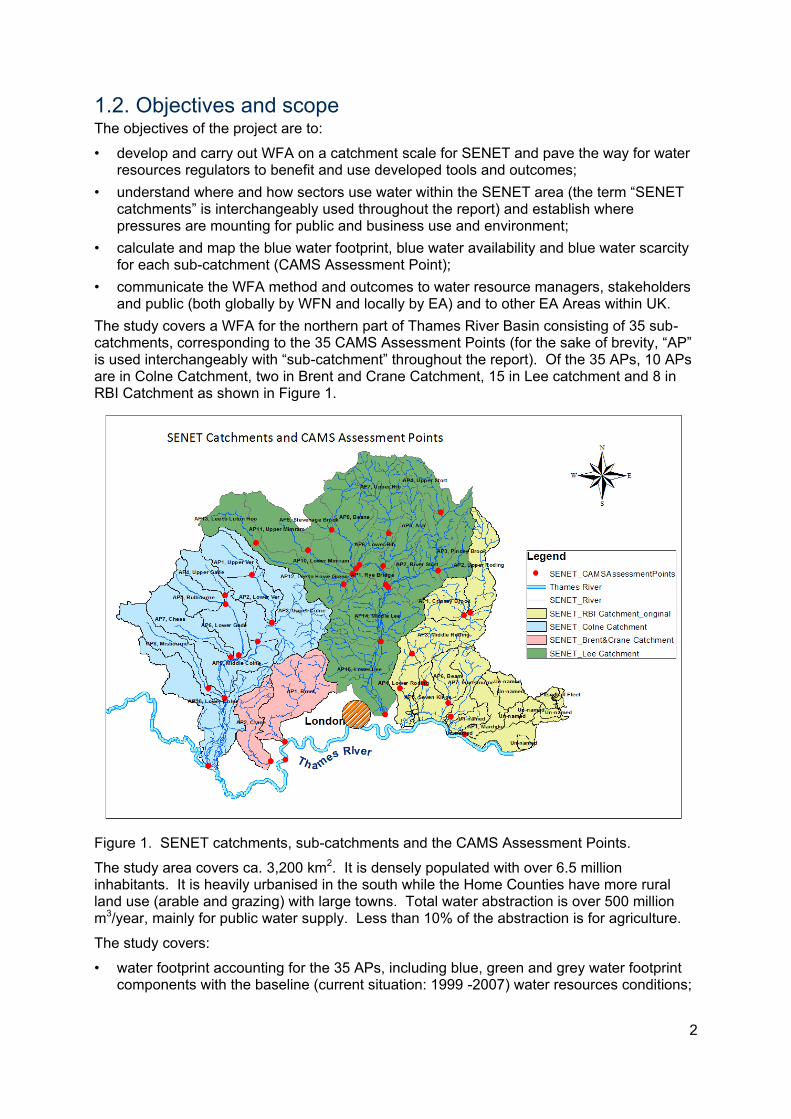
The study covers a WFA for the northern part of Thames River Basin consisting of 35 sub-catchments, corresponding to the  35  CAMS  Assessment  Points  (for  the  sake  of  brevity,  “AP”  is  used  interchangeably  with  “sub-catchment”  throughout  the  report).    Of  the  35  APs,  10  APs  are in Colne Catchment, two in Brent and Crane Catchment, 15 in Lee catchment and 8 in RBI Catchment as shown in Figure 1.

Figure 1. SENET catchments, sub-catchments and the CAMS Assessment Points.

The study area covers ca. 3,200 km2. It is densely populated with over 6.5 million inhabitants. It is heavily urbanised in the south while the Home Counties have more rural land use (arable and grazing) with large towns. Total water abstraction is over 500 million m3/year, mainly for public water supply. Less than 10% of the abstraction is for agriculture.

The study covers:

• water footprint accounting for the 35 APs, including blue, green and grey water footprint components with the baseline (current situation: 1999 -2007) water resources conditions;

3

• water footprint sustainability assessment for the 35 APs - blue water availability, blue water scarcity and water pollution level for both surface water and groundwater;

• water footprint and sustainability projection with climate change and water demand scenarios (2060); and

• recommendations for response strategies for water resources management using the WFA findings.

1.3. This report This report documents the output of the full scope of this WFA study: baseline water footprint accounting, blue water scarcity and water pollution level assessment, projection of the WF and blue water scarcity with the climate change and future water abstraction scenarios for the 35 sub-catchments in the SENET. Chapter 1 introduces the project with the background, objective and scope of the study. Chapter 2 describes the water footprint concept and the Water Footprint Assessment approach in brief, followed by the description on the methods for water footprint accounting, water footprint sustainability assessment and the approaches and key assumptions applied in this study. Chapter 3 presents the results and findings of this Water Footprint Assessment study. Chapter 4 summarises the conclusions followed by recommendations for water footprint response strategies in Chapter 5.

2. Method and data 2.1. Water Footprint Assessment This study follows the general methodology for Water Footprint Assessment described in the Global Water Footprint Assessment Standard as developed by WFN (Hoekstra et al., 2011). The water footprint (WF) is an indicator of freshwater use that looks at both direct and indirect water use of a consumer or producer (Hoekstra et al. 2011). The WF of an individual, community or business is defined as the total volume of freshwater that is used to produce the goods and services consumed by the individual or community or produced by the business. Water use is measured in terms of water volumes consumed (evaporated) and/or polluted per unit of time. A WF can be calculated for a particular product, or any well-defined group of consumers (e.g. an individual, family, village, city, province, state or nation) or producers (e.g. a public organization, private enterprise or economic sector), or for a geographically delineated area (e.g. a river catchment). The WF is a geographically and temporally explicit indicator, showing not only the volumes of the consumptive water use and pollution, but also the locations and time. The WF is a more comprehensive indicator of freshwater resources appropriation, in contrast to the traditional measure of water withdrawal (Figure 2). This study focused on the water footprint within SENET catchment area (see Section 2.2.2) while the water footprint of the catchments from the consumption perspective was preliminarily assessed (Section 3.4).

4

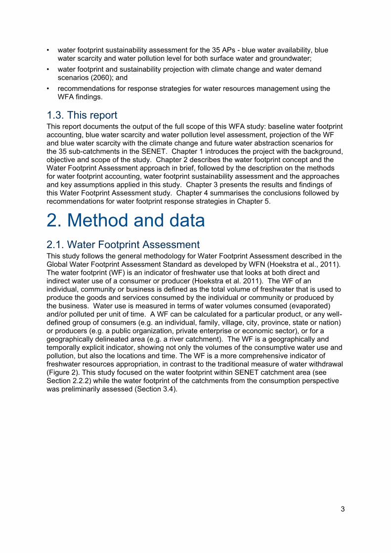
Figure 2. Schematic representation of the components of a water footprint (Hoekstra et al., 2011).

As shown in the above figure, a WF consists of three components: green WF, blue WF and grey WF.

The blue WF measures consumptive use of fresh surface and / or groundwater, the so-called blue  water.    The  term  ‘consumptive  water  use’  refers  to  one  of  the  following  four  cases:  1)  water evaporates; 2) water is incorporated into the product; 3) water does not return to the same catchment area, for example, it is returned to another catchment area or the sea; 4) water does not return in the same period, for example, it is withdrawn in a scarce period and returned in a wet period.

The green WF quantifies the human consumption of the so-called green water. Green water is the part of the precipitation stored in the soil or which temporarily stays on top of the soil or vegetation. The green WF is particularly relevant for agricultural and forestry products (products based on crops or wood). It refers to the total rainwater evapotranspiration (from fields and plantations) plus the water incorporated into the harvested crop or wood.

The grey WF indicates the volume of freshwater that is required to assimilate the load of pollutants based on natural background concentrations and existing ambient water quality standards.

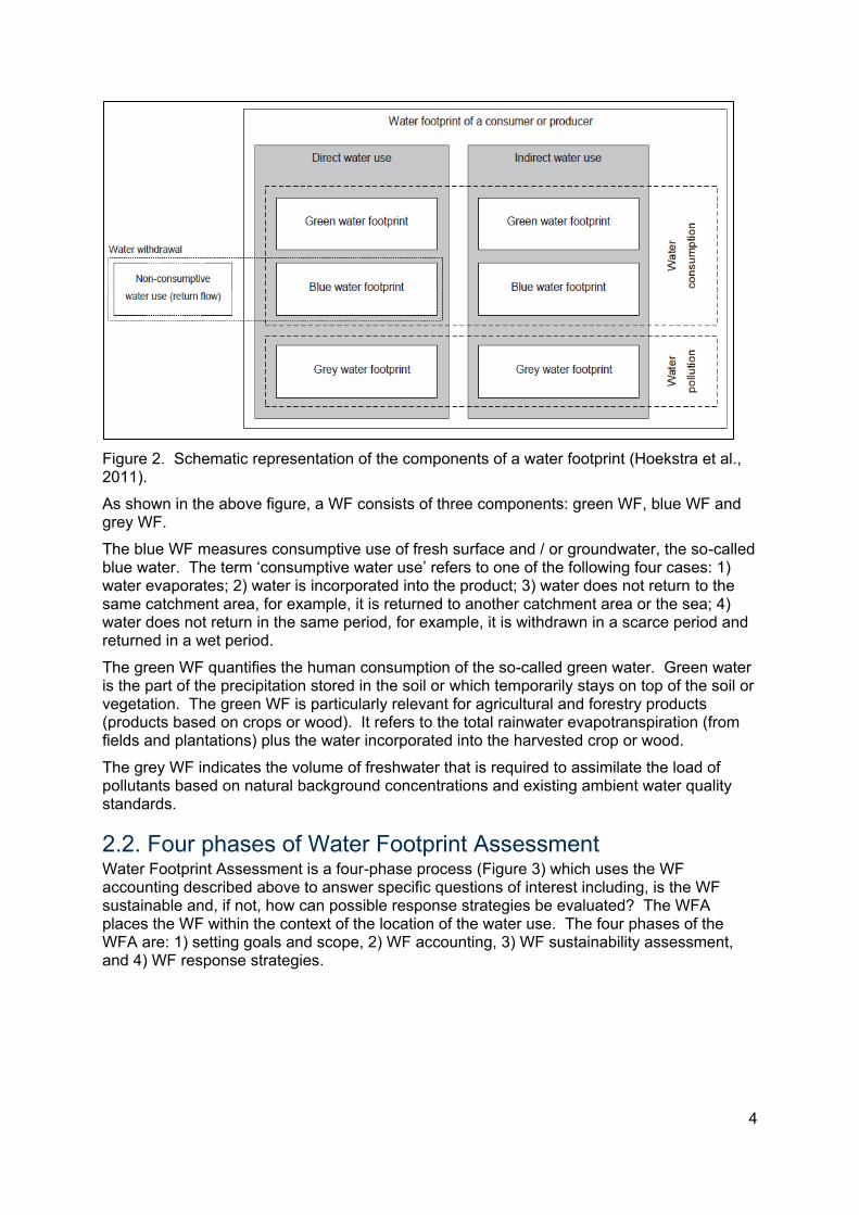
2.2. Four phases of Water Footprint Assessment Water Footprint Assessment is a four-phase process (Figure 3) which uses the WF accounting described above to answer specific questions of interest including, is the WF sustainable and, if not, how can possible response strategies be evaluated? The WFA places the WF within the context of the location of the water use. The four phases of the WFA are: 1) setting goals and scope, 2) WF accounting, 3) WF sustainability assessment, and 4) WF response strategies.

5

Figure 3. Four distinct phases in Water Footprint Assessment (Hoekstra et al., 2011).

2.2.1. Water footprint accounting The blue WF of a process, WFproc_blue (volume/time), is an indicator of consumptive use of blue water, namely, the fresh surface water or groundwater. The blue WF of a process step is calculated as:

WFproc_blue = BlueWaterEvaporation + BlueWaterIncorporation + LostReturnflow (1)

When surface water and groundwater are to be distinguished in blue WF quantification, the above equation can be rewritten as:

WFproc_blue_surf = BlueSurfWaterEvaporation + BlueSurfWaterIncorporation + LostReturnflow (2)

WFproc_blue_ground = BlueGroundWaterEvaporation + BlueGroundWaterIncorporation + GrWaterAbstrToSurfNotReturn (3)

Where WFproc_blue_surf and WFproc_blue_ground are the blue surface WF and blue groundwater footprint, respectively. BlueSurfWaterEvaporation is (blue) surface water evaporation; BlueSurfWaterIncorporation is (blue) surface water incorporated into the product; LostReturnflow is the amount of water after use which does not return to the same catchment in the same period of the water abstraction.

Similarly, BlueGroundWaterEvaporation and BlueGroundWaterIncorporation refer to the (blue) groundwater evaporation and the amount of groundwater incorporated into the product during the process, respectively. GrWaterAbstrToSurfNotReturn is an estimate of the amount of groundwater which does not recharge into the same groundwater system, and/or within the same period under study after abstraction.

The green WF of a process, WFpro_green (volume/time), refers to the total evapotranspiration (GreenWaterEvaporation) of rainwater stored in soil plus the water incorporated into the harvested crop or wood (GreenWaterIncorporation). The green WF of a process step is calculated by:

WFproc_green = GreenWaterEvaporation + GreenWaterIncorporation (4)

The grey WF of a process, WFproc_grey (volume/time), is calculated by:

WFproc_grey = L

max nat (5)

where L (mass/time) is the load of the pollutant under study; cmax (mass/volume) is the maximum acceptable concentration specified by the ambient water quality standard in consideration, and cnat (mass/volume) is the natural background concentration of that pollutant in the receiving water body.

In the case of point sources of water pollution, i.e., when pollutants are directly released into a surface water body in the form of a treated or non-treated wastewater disposal, the grey WF can be estimated by:

WFproc_grey_point = Effl∙ effl Abstr∙ act

max nat (6)

6

where Effl (volume/time) is the discharge rate of effluent while Abstr (volume/time) is the abstraction rate. ceffl and cact are the concentrations of the pollutant under study in the effluent and in the source water of abstraction, respectively.

In the case of diffuse source pollution, the grey water footprint is estimated using

WFproc_grey_diffuse=α∙Appl

max nat (7)

where α is the leaching-run-off fraction. It represents the fraction of applied chemicals (e.g. fertiliser) on land eventually reaching freshwater bodies after land-soil-water interactions. Appl (mass/time/area) is the application of the chemicals on land or into the soil.

The above equations for grey WF can also be applied to groundwater. In such a case, the groundwater quality standards should be used in determining cmax, cact and cnat related to the groundwater system in question.

2.2.2. Water footprint within a catchment In calculating the WF for a geographic area or a hydrological unit such as a sub-catchment, catchment or river basin, all of the processes that are conducted in that hydrological unit will be cumulatively added to determine the total WF for that hydrological unit.

The WF within a catchment (or any geographically delineated area), WFarea (volume/time), is calculated as the sum of the process WFs of all water using processes in the area:

WFarea = ∑ WFproc[𝑖] (8)

where WFproc [i] (volume/time) refers to the WF of a process i within the catchment (area). The equation sums all water-consuming or polluting processes taking place in the area.

2.2.3. Water footprint sustainability assessment Sustainability of a WF can be assessed from an environmental, social and economic perspective. When assessing the WF sustainability, sustainability indicators and the criteria for the assessment need to be established. Blue water scarcity (BWS) and water pollution level (WPL), which are related to blue WF and grey WF, respectively, are the environmental sustainability indicators commonly applied in WFA.

Blue water scarcity BWS in a catchment is defined as the ratio of the total of blue WF in the catchment to the blue water availability of the catchment (Hoekstra et al., 2011). It is expressed by:

WSblue[x,t] = ∑WFblue[x,t]WAblue[x,t]

(9)

where WSblue is the BWS in a catchment x in a certain period t, ΣWFblue is the total blue water footprint in the catchment in that period, and WAblue is the blue water availability.

The blue water availability (WAblue) in a catchment x in a certain period t is quantified by the difference between the natural run-off in the catchment and the environmental flow requirement (EFR), which can be expressed by:

WAblue[x,t] = Rnat[x,t] − EFR[x,t]       (10)

where Rnat is the natural run-off of the catchment in the period under study.

The above equations for sustainability assessment are in a general form when surface and groundwater  are  not  distinguished  within  the  “blue  water”  context.  However,  when  evaluating  water availability and scarcity for surface water and groundwater separately, the above two equations need to modified for the groundwater case.

In this study, Equation 9 will be applied in assessing the overall blue water scarcity that includes the effect of both surface water footprint and groundwater footprint on the total water availability.

7

Blue groundwater availability and scarcity Blue groundwater availability can be approximated by the sustainable yield. The sustainable yield has been discussed and elaborated in a range of studies (e.g. Sophocleous, 2000; Alley and Leake, 2004; Kalf and Woolley, 2005). The sustainable yield concept has evolved from the safe yield concept. However, there is not yet a common consensus on one definition of the sustainable yield. Nevertheless, it is generally regarded as the amount of groundwater that could be abstracted without exceeding the natural recharge or harming the groundwater system from environmental, economic, or social considerations in a long-term perspective (e.g. Alley et al., 1999; Zhou, 2009). Therefore, the blue groundwater water availability is defined as:

WAblue_ground [x,t]=Ps [x,t] (11)

in which

Ps[x,t]=Rsn[x,t]-Oenv[x,t] (12)

where WAblue_ground (volume/time) is the blue groundwater availability in a catchment x in a certain period t; Ps (volume/time) is the sustainable groundwater yield; Rsn (volume/time) is the sustainable natural recharge, which is the sum of natural recharge and the increased recharge induced by abstraction (groundwater pumping). Oenv (volume/time) is the residual discharge or outflow. Both Rsn and Oenv in the context of  “sustainable  groundwater  development”  should  take the ecological or environmental requirements into account when they are estimated. One can refer to Kalf and Woolley (2005) and Zhou (2009) for a more comprehensive description on the sustainable yield and groundwater sustainability.

The blue groundwater scarcity WSblue_ground [-] is defined as the ratio of the total of blue groundwater water footprints, ΣWFblue_ground, to the blue groundwater water availability in the catchment, which is described as

WSblue_ground[x,t] =∑WFblue_ground[x,t]WAblue_ground[x,t]

(13)

Water pollution level Water pollution level (WPL) is defined as the fraction of the waste assimilation capacity consumed. For a WPL of surface water, WPLsurf [x,t], it is calculated by taking the ratio of the total grey water footprints on surface water (WFgrey_surf) in a catchment to the actual runoff (Ract) of that catchment.

WPLsurf[x,t] =∑WFgrey_surf[x,t]

Ract[x,t] (14)

When evaluating the WPL for groundwater, it can be represented by

WPLground[x,t] =∑WFgrey_ground[x,t]

Gact[x,t] (15)

where WPLground (volume/time) is the groundwater WPL in a catchment x in a certain period t; WFgrey_ground is the groundwater grey WF in catchment x in the time t; Gact is the actual groundwater flow of the catchment x at the time t. In the study, WF sustainability assessment was carried out using BWS and WPL and WF hotspots were identified. Hotspots are the areas (APs in this case) where the blue WF of the AP is larger than the blue water availability of the AP and/or the grey WF of the AP exceeds the assimilation capacity for water pollution of the AP, therefore indicating that the blue WF and/or the grey WF are unsustainable, respectively.

2.2.4. Water footprint response strategy Based on the findings of this study, particularly the WF hotspot identification regarding BWS and WPL, suggestions and recommendations will be put forward. The suggestions are made

8

to feed the discussion on visioning and strategising the water resources and abstraction management in the study area and even the whole EA management domain.

2.3. Data The data used in this study were obtained from various sources. The data content and sources are summarised in Table A1 in the Annex.

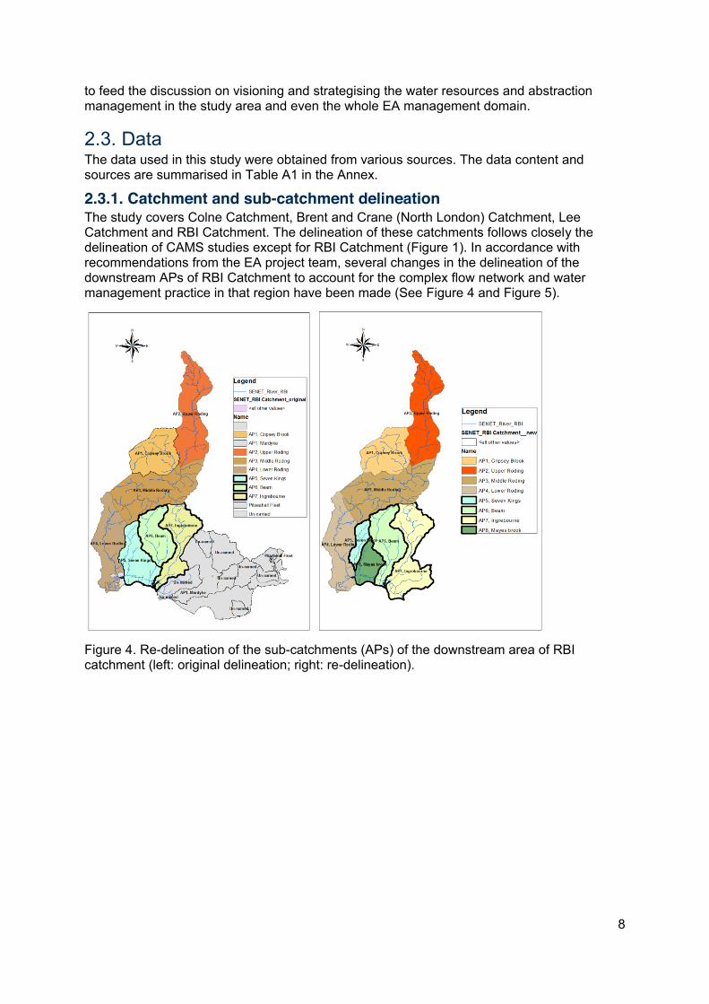
2.3.1. Catchment and sub-catchment delineation The study covers Colne Catchment, Brent and Crane (North London) Catchment, Lee Catchment and RBI Catchment. The delineation of these catchments follows closely the delineation of CAMS studies except for RBI Catchment (Figure 1). In accordance with recommendations from the EA project team, several changes in the delineation of the downstream APs of RBI Catchment to account for the complex flow network and water management practice in that region have been made (See Figure 4 and Figure 5).

Figure 4. Re-delineation of the sub-catchments (APs) of the downstream area of RBI catchment (left: original delineation; right: re-delineation).

9

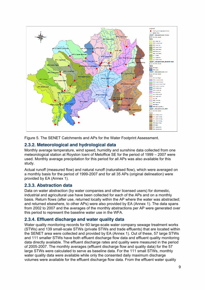
Figure 5. The SENET Catchments and APs for the Water Footprint Assessment.

2.3.2. Meteorological and hydrological data Monthly average temperature, wind speed, humidity and sunshine data collected from one meteorological station at Royston Iceni of Metoffice SE for the period of 1999 – 2007 were used. Monthly average precipitation for this period for all APs was also available for this study.

Actual runoff (measured flow) and natural runoff (naturalised flow), which were averaged on a monthly basis for the period of 1999-2007 and for all 35 APs (original delineation) were provided by EA (Annex 1).

2.3.3. Abstraction data Data on water abstraction (by water companies and other licensed users) for domestic, industrial and agricultural use have been collected for each of the APs and on a monthly basis. Return flows (after use, returned locally within the AP where the water was abstracted; and returned elsewhere, to other APs) were also provided by EA (Annex 1). The data spans from 2002 to 2007 and the averages of the monthly abstractions per AP were generated over this period to represent the baseline water use in the WFA.

2.3.4. Effluent discharge and water quality data Water quality monitoring records for 60 large-scale water company sewage treatment works (STWs) and 139 small-scale STWs (private STWs and trade effluents) that are located within the SENET area were collected and provided by EA (Annex 1). Out of these, 57 large STWs and 111 smaller STWs have both effluent discharge flow data and effluent quality monitoring data directly available. The effluent discharge rates and quality were measured in the period of 2005-2007. The monthly averages (effluent discharge flow and quality data) for the 57 large STWs were calculated to serve as baseline data. For the 111 small STWs, monthly water quality data were available while only the consented daily maximum discharge volumes were available for the effluent discharge flow data. From the effluent water quality

10

monitoring data, ammonia-nitrogen (NH4+-N), arsenic (As), boron (B), cadmium (Cd), chloride (Cl-), chromium (taken as Cr6+), copper (Cu), lead (Pb), mercury (Hg) , nickel (Ni), total oxidised nitrogen-N and reactive orthophosphate-P are the dominant pollutants.

There are 171 point-source effluents registered within the SENET catchments that are directly or indirectly discharged to groundwater. These discharges can potentially generate a grey WF on groundwater. The data available for these discharges are the consented daily maximum discharge volumes and estimated average concentrations for ammonia-nitrogen (NH4+-N).

2.3.5. Agricultural, soil and agro-chemical data Several crops, such as wheat, barley (winter and spring barley), potato, sugar beet, rapeseed, maize, pea, beans, and vegetables and fruits are grown in the SENET catchments. Cultivation area of each of these crops was available. The yield data, however, were available for only five crops, i.e. wheat, barley potato, sugar beet and rapeseed. There are also animal farms in the study area; however, data for the animal product WF accounting is insufficient. The information on soil type was acquired (Annex 1). Nitrogen and phosphorous fertiliser application in farm lands and leaching rate of these fertilisers were derived from the data or literature (Davison et al., 2008; Mekonnen and Hoekstra, 2011).

2.3.6. Population and other data Population data (UK 2001 census data) for each village and town in the SENET APs have been collated and aggregated to the AP level. These data were only used for consumption water footprint calculation for the SENET catchments. The WF of national consumption for UK has been taken from the Waterstat Database (http://www.waterfootprint.org/?page=files/WaterStat); see also Hoekstra and Mekonnen (2012).

2.4. Approach and key assumptions The application of the WFA in the project catchments are described in the following sections. The assessment was carried out at the sub-catchment (AP) level and monthly time scale.

2.4.1. Baseline blue water footprint accounting Water used for industrial, domestic and agricultural purposes is included in the WFA whether it is abstracted directly from surface water or groundwater bodies or supplied by water companies. The WF was calculated for all three sectors and with respect to the two blue water sources. For a sub-catchment (AP), the total blue WF (WF_blue) is the difference between the total water abstraction (ABS) within the AP and the total flow locally returned (RTN_local) within the AP, expressed as follows in a generic formula.

WF_blue = ABS – RTN_local (16)

One can apply this general equation to the WF calculation for the above mentioned water use sectors using different sources of blue water, namely

WF_blue_surf _indus = ABS_surf _indus – RTN_local_surf _indus (17)

WF_blue_surf _domes = ABS_surf _domes – RTN_local_surf _domes (18)

WF_blue_grw _indus = ABS_grw _indus – RTN_local_grw _indus (19)

WF_blue_grw _domes = ABS_grw _domes – RTN_local_grw _domes (20)

In the above expressions, _surf and _grw stand for surface water and groundwater sources, respectively; _indus and _domes stand  for  “industrial”  and  “domestic”,  respectively.

For the blue WF, evaporative water consumption and non-evaporative consumption were calculated separately. The former was estimated by

WF_blue (evaporative) = ABS – RTN_local – RTN_elsewhere (21)

11

where RTN_elsewhere refers to the flows returned to a different AP, namely the so-called “lost  return  flow”.  The  non-evaporative consumption was estimated by

WF_blue (non-evaporative) = RTN_elsewhere (22)

Equation 21 and 22 were applied separately for surface water and groundwater sources and for the above three water use sectors.

For agriculture, although the total water abstraction for agricultural use (irrigation) was available, the actual return flow data from the farm areas were unknown. In addition, types of crops and areas of crop growing are different from AP to AP; the consumption of water (both blue and green water) by different crops varies significantly. Consequently, a direct estimation of blue WF for agriculture is not possible. Therefore the blue WF for agriculture was evaluated using the CROPWAT model (Allen et al., 1998; Doorenbos et al., 1986; http://www.fao.org/nr/water/infores_databases_cropwat.html) with an assumption that these five crops are all cultivated using a combination of rainfall and irrigation. The calculation of the blue WF of crops with CROPWAT model is described in the section 2.4.3. The modelled blue water footprint for agriculture was adjusted using the abstraction data (i.e. water abstracted for agriculture use). The post-modelling adjustment was based on the criterion that the modelled blue WF should not be larger than the abstraction for agriculture use (irrigation).

2.4.2. Lost return flow The lost return flow of one AP is a component of the total blue WF of the AP under study. No data was available indicating the location and volumes of water transfer between APs. The water transfers between APs were derived based on the following approach. We assumed that the lost return flows from industrial and domestic use of one AP would be captured by the sewage treatment works (STWs). To identify movement of the lost return flows between APs (i.e. identify the APs receiving the lost return flows), the sewerage catchment map of STWs that are managed by Thames Water was used. This map describes the coverage of the  STW’s  service  region  and  area.  The  proportion  of  the  service  area  was  used  to  calculate  the amount of the lost return flow being received by the relevant APs. For example, if AP1 is served by the STWs in AP2 and AP3, and 50% of the service area of AP1 is covered by the STWs in AP2 and the other 50% is covered by the STWs in AP3, then the lost return flow of AP1 is to be split proportionally between these two receiving APs. This means that AP2 receives 50% of the lost return flow from AP1 and AP3 receives the other 50% of the lost return flow of AP1.

2.4.3. Baseline green water footprint accounting Crop growth uses green water from rainfall and blue water supplied by irrigation when soil water deficit arises. Therefore, the total crop water consumption, or crop water use (CWU), consists of green and blue water use, i.e., crop evapotranspiration using green water (rainfall stored in soil), ET_green, and crop evapotranspiration using blue water (irrigation), ET_blue.

CWU is expressed by

CWU = ET_green + ET_blue (23)

ET_green is generally estimated by

ET_green = min (ET_c, P_eff) (24)

Where ET_c is the actual crop evapotranspiration (Allen et al., 1998), min is minimum, and P_eff is the effective precipitation. Hence, the green WF for each crop can be obtained by

WF_green (crop) = ET_green (25)

The blue WF for each crop can be obtained by

WF_blue (crop) = ET_blue (26)

12

The green WF of an AP, WF_green (AP), is obtained by a summation of the green WF of each crop grown in that AP, namely

WF_green  (AP)  =  Σ  [WF_green  (cropi)  ],  (i=1,2…n) (27)

where WF_green (cropi) is the green WF of ith crop cultivated in the AP in question.

The green WF was computed by applying the CROPWAT model for each AP in the SENET catchments taking into account five crops: wheat, barley (winter and spring barley), potato, sugar beet and rapeseed, for which the cultivation area and yield data could be obtained. In the model, “irrigation  scheduling”  option  was  applied.  Since  no  actual  irrigation  scheduling  data for each of those crops were available, it was assumed in the model that irrigation would take place at 100% depletion and irrigate to 100% field capacity. Local meteorological data, precipitation and soil data were used in the model computation (see Annex 1).

The calculation of blue and green WF was done on a daily basis, however CROPWAT provides only daily total crop water use (CWU), i.e. the daily total evapotranspiration in the entire growing period, which includes ET_green and ET_blue. Therefore a post-model processing, applying the Equations (23) – (27), was done to generate monthly WF results for the crops.

2.4.4. Baseline grey water footprint accounting Grey WF resulting from point source effluent discharges was estimated for both surface water and groundwater. There are 60 large-scale STWs and 139 small-scale STWs (private STW and trade effluents) distributed in the study area. For these STWs, some are lacking water quality data while some are lacking discharge quantity data. As a result, the grey WFs was estimated for 57 large-scale STWs and 111 small-scale STWs because these STWs have both discharge and water quality monitoring data in the same period. Those STWs without either discharge volume or water quality data were neglected in the grey WF assessment in this study. As a result this leads to certain underestimation of the pollution load, thus the grey WF. The grey WF was calculated by applying Equation (5) in which the load of the pollutant under study, L, is estimated by

L = ceff x Deffl (28)

where ceff and Deffl are the concentration (mass/volume) of the pollutant in the effluent and the effluent discharge rate (volume/time), respectively.

The grey WF was estimated separately for each STW with respect to 12 pollutants (or water quality determinants) which were evaluated individually. These determinants, as described above, are ammonia nitrogen (NH4+-N), arsenic (As), boron (B), cadmium (Cd), chloride (Cl-), chromium (taken as Cr6+), copper (Cu), lead (Pb), mercury (Hg) , nickel (Ni), total oxidised nitrogen (taken as dissolved inorganic nitrogen, DIN), and reactive orthophosphate (taken as dissolved reactive phosphate DRP or in another term dissolved inorganic phosphate, DIP). After this evaluation, the largest grey WF (WF_grey) of all 12 determinants was taken as the grey WF for the STW under study. Subsequently, the grey WFs of all the STWs located in one AP were summed up to obtain the grey WF for that AP.

This can be expressed as follows:

WF_grey (STWi) = Max[WF_grey (pj)], (i=1,2,…n,  j=1,2…m) (29)

WF_grey  (AP)  =  Σ[WF_grey  (STWi) ], (i=1,2…n) (30)

where STWi stands for the ith sewage treatment work (STW) and pj stands for the jth pollutant.

The grey WFs for all 57 large STWs were calculated at a monthly time scale. For the 111 small STWs, the monthly effluent discharge volume was estimated with the assumption that these STWs discharge every day at the maximum consented volume. This could

13

overestimate the grey WF. The grey WFs of the 111 small STWs were also estimated in this way on the monthly basis.

Grey WF for groundwater due to point source discharge was estimated applying the same approach as described above. The grey WF for groundwater was calculated with respect to NH4+-N based on the consented maximum daily discharge volume and the consented concentration of NH4+-N (10 mg/l). In this study, discharges of pollutants into groundwater were  categorized  as  “onto  land”,  “into  land”,  “soak-away”,  “underground  water”,  “irrigation  area”  and  “pipe”.  For  the  discharges  with  “into  land”,  “soak-away”,  “underground  water”  and  “pipe”,  it  was  assumed  100%  of  the  pollutant  load  would  be  added to the groundwater aquifers since these types of effluent directly enter the groundwater system. For those of “onto  land”  and  “irrigation  area”,  it  was  assumed  80%  of  the  loads  would  eventually  reach  the  groundwater systems. This assumption was based on the information that in average the potential infiltration rate in this region is ca. 200 mm/year (British Geological Survey) while the average effective rainfall is 250 mm/year (Bloomfield et al., 2011). From there one can see that a maximum of 80% of the volume of water applied to land surface could potentially reach groundwater. This preliminary estimation gives a worse scenario, which is a precautionary approach. However, STWs that are not maintained properly often discharge a far worse water quality.

The grey WF non-point source pollution from agriculture, WF_grey (agri), was estimated with respect to nitrogen (N) and phosphorous (P). WF_grey (agri) is a result of leaching of fertilisers applied in crop lands,. The estimation was done using Equation 7. In the estimation, the application rate of N and P applied to crop lands was estimated based on the modelling study of Davison et al. (2008). The assumed nutrients’ runoff-leaching rates, 10% for N and 5% for P, were based on Mekonnen and Hoekstra (2011). The calculated WF_grey (agri) was taken as a grey WF on surface water since the runoff-leaching rate is a lumped parameter without an explicit partition between the leaching to surface water and that to groundwater.

Maximum allowable concentration cmax and natural background concentration cnat and the associated assumptions are presented in the following Section 2.4.4 (Table 1).

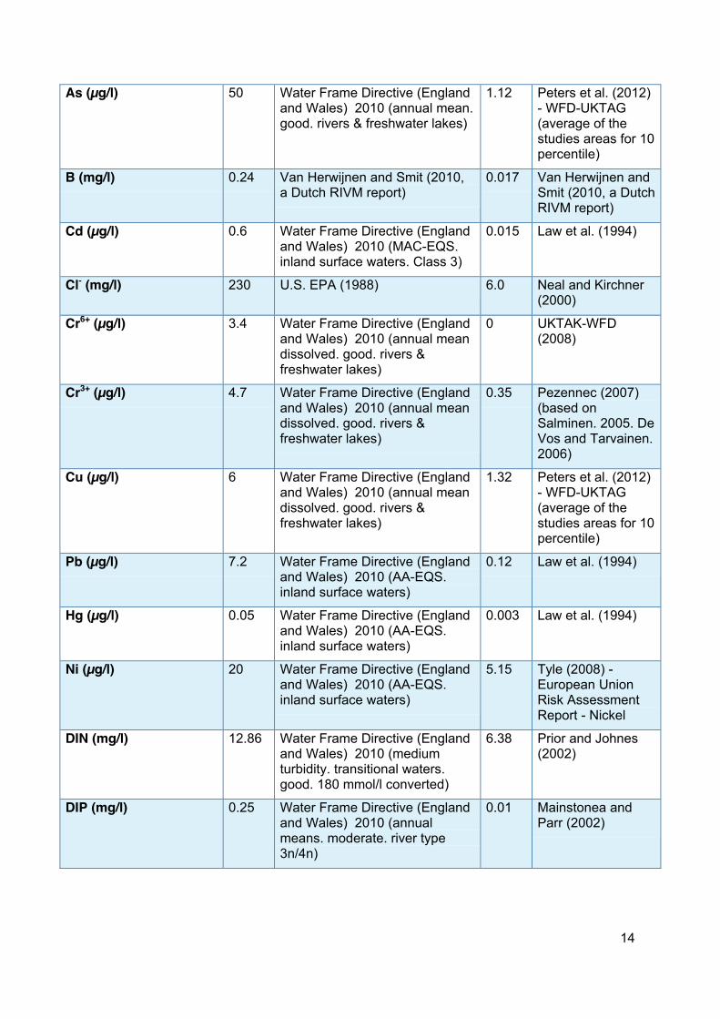
2.4.5. Chosen water quality standards and natural background concentrations Various literature sources and legislation documents of the UK government have been studied to obtain the maximum allowable concentration (cmax) and natural background concentration (cnat) for the above listed 12 water quality determinants. Since UK is a member country of EU and has to meet the water quality targets of the EU Water Framework Directive (WFD), the water quality standards for the determinants as stipulated in the WFD for England and Wales were applied as cmax. For those determinants, in this case B and Cl-, which are not listed in the WFD standards, cmax values were taken from literature. Natural background concentration values of these 12 determinants were mostly sourced from the research literature relevant to UK. The values of cmax and cnat and literature sources are presented in Table 1.

Table 1. Values of cmax and cnat for surface water and groundwater and literature sources.

Water Quality determinants

cmax Sources for cmax cnat Sources for cnat

NH4+_N (mg/l)

Surface water 0.3 Water Frame Directive (England and Wales) 2010 (90-percentile. good. river type 1.2.4.6)

0.01 Reynolds and Edwards (1994)

Groundwater 0.29 Water Frame Directive (England and Wales) 2010 (General quality of groundwater body)

0.14 Shand et al. (2007)

14

As (µg/l) 50 Water Frame Directive (England and Wales) 2010 (annual mean. good. rivers & freshwater lakes)

1.12 Peters et al. (2012) - WFD-UKTAG (average of the studies areas for 10 percentile)

B (mg/l) 0.24 Van Herwijnen and Smit (2010, a Dutch RIVM report)

0.017 Van Herwijnen and Smit (2010, a Dutch RIVM report)

Cd (µg/l) 0.6 Water Frame Directive (England and Wales) 2010 (MAC-EQS. inland surface waters. Class 3)

0.015 Law et al. (1994)

Cl- (mg/l) 230 U.S. EPA (1988) 6.0 Neal and Kirchner (2000)

Cr6+ (µg/l) 3.4 Water Frame Directive (England and Wales) 2010 (annual mean dissolved. good. rivers & freshwater lakes)

0 UKTAK-WFD (2008)

Cr3+ (µg/l) 4.7 Water Frame Directive (England and Wales) 2010 (annual mean dissolved. good. rivers & freshwater lakes)

0.35 Pezennec (2007) (based on Salminen. 2005. De Vos and Tarvainen. 2006)

Cu (µg/l) 6 Water Frame Directive (England and Wales) 2010 (annual mean dissolved. good. rivers & freshwater lakes)

1.32 Peters et al. (2012) - WFD-UKTAG (average of the studies areas for 10 percentile)

Pb (µg/l) 7.2 Water Frame Directive (England and Wales) 2010 (AA-EQS. inland surface waters)

0.12 Law et al. (1994)

Hg (µg/l) 0.05 Water Frame Directive (England and Wales) 2010 (AA-EQS. inland surface waters)

0.003 Law et al. (1994)

Ni (µg/l) 20 Water Frame Directive (England and Wales) 2010 (AA-EQS. inland surface waters)

5.15 Tyle (2008) - European Union Risk Assessment Report - Nickel

DIN (mg/l) 12.86 Water Frame Directive (England and Wales) 2010 (medium turbidity. transitional waters. good. 180 mmol/l converted)

6.38 Prior and Johnes (2002)

DIP (mg/l) 0.25 Water Frame Directive (England and Wales) 2010 (annual means. moderate. river type 3n/4n)

0.01 Mainstonea and Parr (2002)

15

2.4.6. Accounting for the water footprint of consumption The water footprint of consumption per AP, WF_consum (AP), under the baseline condition, was estimated by multiplying the national average consumption water footprint per capita, WF_consum (UK-per-capita), and the population of each AP, Popul (AP). The equation reads:

WF_consum (AP) = WF_consum (UK-per-capita) x Popul (AP) (31)

This estimation is based on the assumption that the consumption pattern for the population in each AP is identical. This is a rough estimation due to the fact that it is very hard to trace the trade flows (import and export) and consumption data of the inhabitants at such a fine geographical unit (AP).

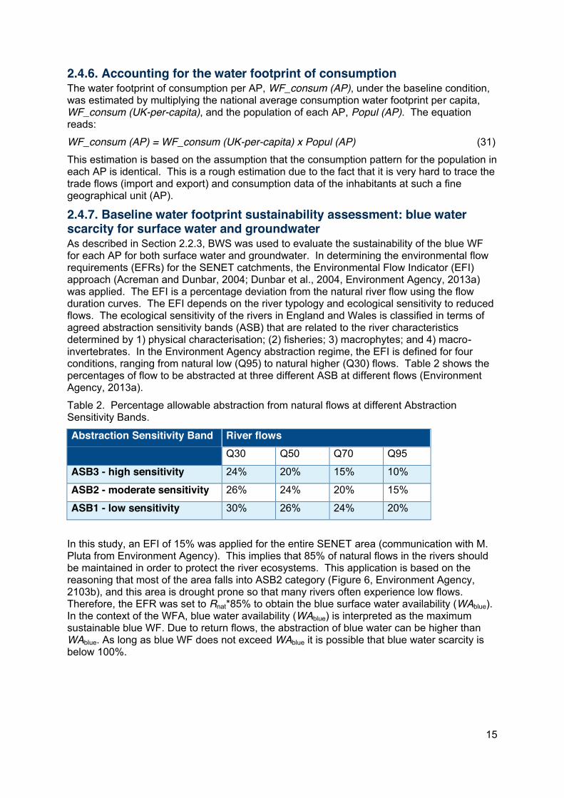
2.4.7. Baseline water footprint sustainability assessment: blue water scarcity for surface water and groundwater As described in Section 2.2.3, BWS was used to evaluate the sustainability of the blue WF for each AP for both surface water and groundwater. In determining the environmental flow requirements (EFRs) for the SENET catchments, the Environmental Flow Indicator (EFI) approach (Acreman and Dunbar, 2004; Dunbar et al., 2004, Environment Agency, 2013a) was applied. The EFI is a percentage deviation from the natural river flow using the flow duration curves. The EFI depends on the river typology and ecological sensitivity to reduced flows. The ecological sensitivity of the rivers in England and Wales is classified in terms of agreed abstraction sensitivity bands (ASB) that are related to the river characteristics determined by 1) physical characterisation; (2) fisheries; 3) macrophytes; and 4) macro-invertebrates. In the Environment Agency abstraction regime, the EFI is defined for four conditions, ranging from natural low (Q95) to natural higher (Q30) flows. Table 2 shows the percentages of flow to be abstracted at three different ASB at different flows (Environment Agency, 2013a).

Table 2. Percentage allowable abstraction from natural flows at different Abstraction Sensitivity Bands.

Abstraction Sensitivity Band River flows Q30 Q50 Q70 Q95

ASB3 - high sensitivity 24% 20% 15% 10%

ASB2 - moderate sensitivity 26% 24% 20% 15%

ASB1 - low sensitivity 30% 26% 24% 20%

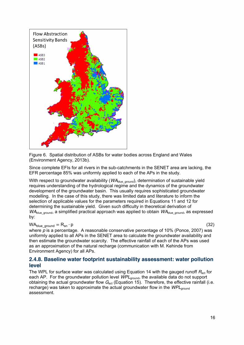
In this study, an EFI of 15% was applied for the entire SENET area (communication with M. Pluta from Environment Agency). This implies that 85% of natural flows in the rivers should be maintained in order to protect the river ecosystems. This application is based on the reasoning that most of the area falls into ASB2 category (Figure 6, Environment Agency, 2103b), and this area is drought prone so that many rivers often experience low flows. Therefore, the EFR was set to Rnat*85% to obtain the blue surface water availability (WAblue). In the context of the WFA, blue water availability (WAblue) is interpreted as the maximum sustainable blue WF. Due to return flows, the abstraction of blue water can be higher than WAblue. As long as blue WF does not exceed WAblue it is possible that blue water scarcity is below 100%.

16

Figure 6. Spatial distribution of ASBs for water bodies across England and Wales (Environment Agency, 2013b).

Since complete EFIs for all rivers in the sub-catchments in the SENET area are lacking, the EFR percentage 85% was uniformly applied to each of the APs in the study.

With respect to groundwater availability (WAblue_ground), determination of sustainable yield requires understanding of the hydrological regime and the dynamics of the groundwater development of the groundwater basin. This usually requires sophisticated groundwater modelling. In the case of this study, there was limited data and literature to inform the selection of applicable values for the parameters required in Equations 11 and 12 for determining the sustainable yield. Given such difficulty in theoretical derivation of WAblue_ground, a simplified practical approach was applied to obtain WAblue_ground, as expressed by:

WAblue_ground = Rsn ∙ p (32) where p is a percentage. A reasonable conservative percentage of 10% (Ponce, 2007) was uniformly applied to all APs in the SENET area to calculate the groundwater availability and then estimate the groundwater scarcity. The effective rainfall of each of the APs was used as an approximation of the natural recharge (communication with M. Kehinde from Environment Agency) for all APs.

2.4.8. Baseline water footprint sustainability assessment: water pollution level The WPL for surface water was calculated using Equation 14 with the gauged runoff Ract for each AP. For the groundwater pollution level WPLground, the available data do not support obtaining the actual groundwater flow Gact (Equation 15). Therefore, the effective rainfall (i.e. recharge) was taken to approximate the actual groundwater flow in the WPLground assessment.

17

2.5. Water footprint projection 2.5.1. Projection scenarios Two climate change scenarios – “wet”  and  “dry”  – were used in combination with projected changes in water abstraction per sector to conduct a WFA for 2060. The existing climate change scenarios and projected water abstraction for agriculture, industry and domestic supply adopted by the EA for the SENET area were the basis for this WFA (communication with C. Beales and G. Frapporti from Environment Agency). Table 3 presents a brief description of the scenarios used in the projection.

Table 3. Projection scenarios for climate change and water abstraction in SENET catchments.

Projection scenarios (2060)

Climate change for natural flows Water abstraction Wet Dry Agriculture Industry Domestic

Modelling output with reference to Mimram (Lee AP10)

Modelling output with reference to Mimram (Lee AP10)

50% increase

25% increase

25% increase

The existing climate change modelling was done only for the Lower Mimram sub catchment (AP10 in Lee Catchment). Assuming the entire SENET area would experience the same climate change pattern, the ratio of projected natural flow to the baseline natural flow at Mimram was applied to all APs in SENET to obtain the natural flow projection. Only one scenario  for  water  abstraction  was  applied  in  this  study  considering  a  “middle”  behaviour  in  terms of water demand and use, which is in between the so-called  “good”  and  “bad”  behaviour (communication with C. Beales from Environment Agency). Bear in mind that the approaches taken in the projection scenarios are very simplified due to the limitation of the data on climate change scenarios and water demand scenarios.

The number of STWs was assumed to remain the same while the effluent discharge volume from each of the STWs was considered to increase in the same percentage as for abstraction. The quality of the effluent discharges was assumed to have no change with reference to the baseline effluent water quality.

2.5.2. Water footprint and sustainability projection Based on Table 3, the blue WF of industrial and domestic sectors for surface and ground water in the future scenario (2060) were assumed to increase by 25%. The flow movement, namely the spatial distribution pattern of the WF due to lost return flow was kept the same as under the baseline condition. The blue WF for agriculture was calculated using the CROPWAT model based on the climate change scenarios and then adjusted with the water abstraction for agricultural use which was projected to increase by 50%.

Similarly as described above, the green WF was projected using the climate change parameters with the CROPWAT model.

For the grey WF projection, it was assumed that only the effluent volume from the STWs would increase by 25% while the quality of the effluents (i.e. the concentrations of the pollutants) would remain the same as under the baseline condition. This implies that the grey WF due to point-sources will be increased by 25% following the increase of the effluent volume by 25%. The grey WF due to diffuse sources was not projected since there was no available data on future cropping changes. However, it was assumed that improved environmental awareness and better technology and practices would result in no significant change in the grey WF resulting from nutrient runoff leaching even with an increase in overall agricultural production.

18

In the projection of blue water scarcity, the future natural flows were estimated based on the climate change modelling for the Mimram catchment (Lee AP10), as described above. It was assumed that the general characteristics of water bodies (rivers etc.) in the SENET area and their ecological sensitivity to water abstraction would not change by 2060; hence the EFRs of the rivers would remain unchanged. The WPLs were not projected due to the unavailability of projected river flows.

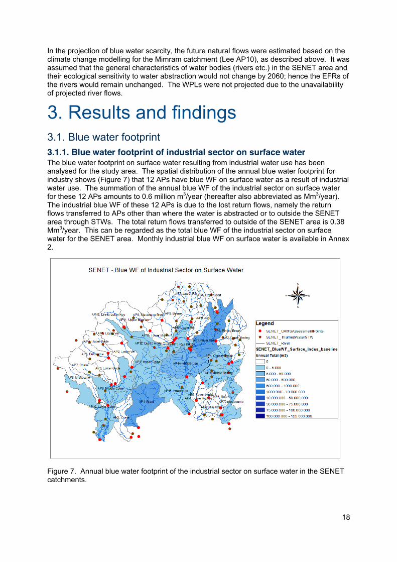
3. Results and findings 3.1. Blue water footprint 3.1.1. Blue water footprint of industrial sector on surface water The blue water footprint on surface water resulting from industrial water use has been analysed for the study area. The spatial distribution of the annual blue water footprint for industry shows (Figure 7) that 12 APs have blue WF on surface water as a result of industrial water use. The summation of the annual blue WF of the industrial sector on surface water for these 12 APs amounts to 0.6 million m3/year (hereafter also abbreviated as Mm3/year). The industrial blue WF of these 12 APs is due to the lost return flows, namely the return flows transferred to APs other than where the water is abstracted or to outside the SENET area through STWs. The total return flows transferred to outside of the SENET area is 0.38 Mm3/year. This can be regarded as the total blue WF of the industrial sector on surface water for the SENET area. Monthly industrial blue WF on surface water is available in Annex 2.

Figure 7. Annual blue water footprint of the industrial sector on surface water in the SENET catchments.

19

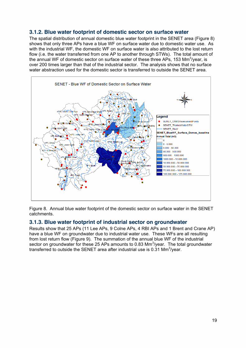
3.1.2. Blue water footprint of domestic sector on surface water The spatial distribution of annual domestic blue water footprint in the SENET area (Figure 8) shows that only three APs have a blue WF on surface water due to domestic water use. As with the industrial WF, the domestic WF on surface water is also attributed to the lost return flow (i.e. the water transferred from one AP to another through STWs). The total amount of the annual WF of domestic sector on surface water of these three APs, 153 Mm3/year, is over 200 times larger than that of the industrial sector. The analysis shows that no surface water abstraction used for the domestic sector is transferred to outside the SENET area.

Figure 8. Annual blue water footprint of the domestic sector on surface water in the SENET catchments.

3.1.3. Blue water footprint of industrial sector on groundwater Results show that 25 APs (11 Lee APs, 9 Colne APs, 4 RBI APs and 1 Brent and Crane AP) have a blue WF on groundwater due to industrial water use. These WFs are all resulting from lost return flow (Figure 9). The summation of the annual blue WF of the industrial sector on groundwater for these 25 APs amounts to 0.83 Mm3/year. The total groundwater transferred to outside the SENET area after industrial use is 0.31 Mm3/year.

20

Figure 9. Annual blue water footprint of the industrial sector on groundwater in the SENET catchments.

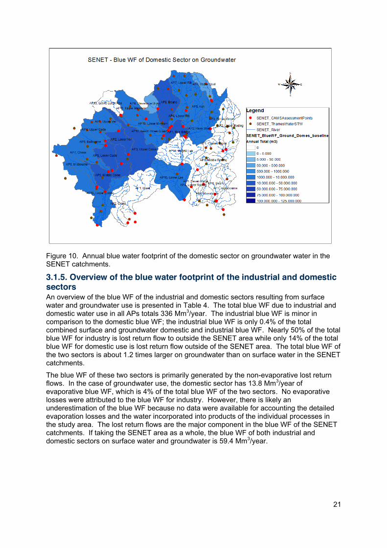
3.1.4. Blue water footprint of domestic sector on groundwater Sixty five percent of the SENET APs, i.e. 22 APs have a blue WF on groundwater due to domestic water use (Figure 10). Ten of these APs are in Colne catchment and 12 APs in Lee catchment. The total WF of the domestic sector on groundwater is around 181 Mm3/year of which 13.8 Mm3/year is due to evaporative loss and 167 Mm3/year is resulting from the lost return flows. The return flows lost to outside the SENET area due to groundwater abstraction for domestic use is 45 Mm3/year.

21

Figure 10. Annual blue water footprint of the domestic sector on groundwater water in the SENET catchments.

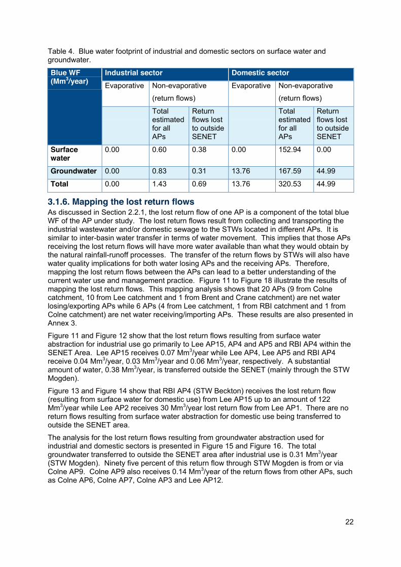
3.1.5. Overview of the blue water footprint of the industrial and domestic sectors An overview of the blue WF of the industrial and domestic sectors resulting from surface water and groundwater use is presented in Table 4. The total blue WF due to industrial and domestic water use in all APs totals 336 Mm3/year. The industrial blue WF is minor in comparison to the domestic blue WF; the industrial blue WF is only 0.4% of the total combined surface and groundwater domestic and industrial blue WF. Nearly 50% of the total blue WF for industry is lost return flow to outside the SENET area while only 14% of the total blue WF for domestic use is lost return flow outside of the SENET area. The total blue WF of the two sectors is about 1.2 times larger on groundwater than on surface water in the SENET catchments.

The blue WF of these two sectors is primarily generated by the non-evaporative lost return flows. In the case of groundwater use, the domestic sector has 13.8 Mm3/year of evaporative blue WF, which is 4% of the total blue WF of the two sectors. No evaporative losses were attributed to the blue WF for industry. However, there is likely an underestimation of the blue WF because no data were available for accounting the detailed evaporation losses and the water incorporated into products of the individual processes in the study area. The lost return flows are the major component in the blue WF of the SENET catchments. If taking the SENET area as a whole, the blue WF of both industrial and domestic sectors on surface water and groundwater is 59.4 Mm3/year.

22

Table 4. Blue water footprint of industrial and domestic sectors on surface water and groundwater.

Blue WF (Mm3/year)

Industrial sector Domestic sector Evaporative Non-evaporative

(return flows)

Evaporative Non-evaporative

(return flows)

Total estimated for all APs

Return flows lost to outside SENET

Total estimated for all APs

Return flows lost to outside SENET

Surface water

0.00 0.60 0.38 0.00 152.94 0.00

Groundwater 0.00 0.83 0.31 13.76 167.59 44.99

Total 0.00 1.43 0.69 13.76 320.53 44.99

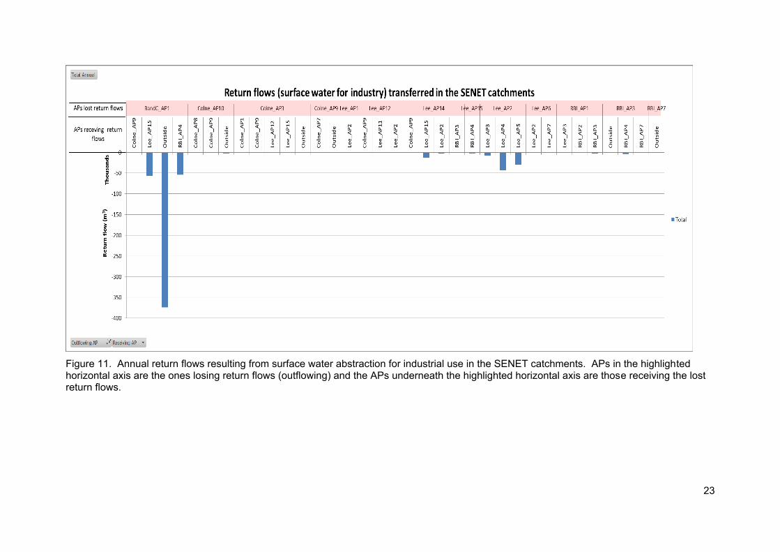
3.1.6. Mapping the lost return flows As discussed in Section 2.2.1, the lost return flow of one AP is a component of the total blue WF of the AP under study. The lost return flows result from collecting and transporting the industrial wastewater and/or domestic sewage to the STWs located in different APs. It is similar to inter-basin water transfer in terms of water movement. This implies that those APs receiving the lost return flows will have more water available than what they would obtain by the natural rainfall-runoff processes. The transfer of the return flows by STWs will also have water quality implications for both water losing APs and the receiving APs. Therefore, mapping the lost return flows between the APs can lead to a better understanding of the current water use and management practice. Figure 11 to Figure 18 illustrate the results of mapping the lost return flows. This mapping analysis shows that 20 APs (9 from Colne catchment, 10 from Lee catchment and 1 from Brent and Crane catchment) are net water losing/exporting APs while 6 APs (4 from Lee catchment, 1 from RBI catchment and 1 from Colne catchment) are net water receiving/importing APs. These results are also presented in Annex 3.

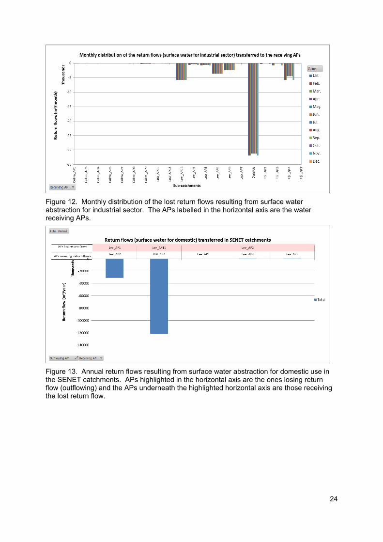
Figure 11 and Figure 12 show that the lost return flows resulting from surface water abstraction for industrial use go primarily to Lee AP15, AP4 and AP5 and RBI AP4 within the SENET Area. Lee AP15 receives 0.07 Mm3/year while Lee AP4, Lee AP5 and RBI AP4 receive 0.04 Mm3/year, 0.03 Mm3/year and 0.06 Mm3/year, respectively. A substantial amount of water, 0.38 Mm3/year, is transferred outside the SENET (mainly through the STW Mogden).

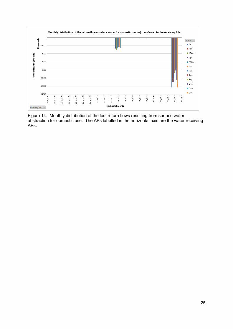
Figure 13 and Figure 14 show that RBI AP4 (STW Beckton) receives the lost return flow (resulting from surface water for domestic use) from Lee AP15 up to an amount of 122 Mm3/year while Lee AP2 receives 30 Mm3/year lost return flow from Lee AP1. There are no return flows resulting from surface water abstraction for domestic use being transferred to outside the SENET area.

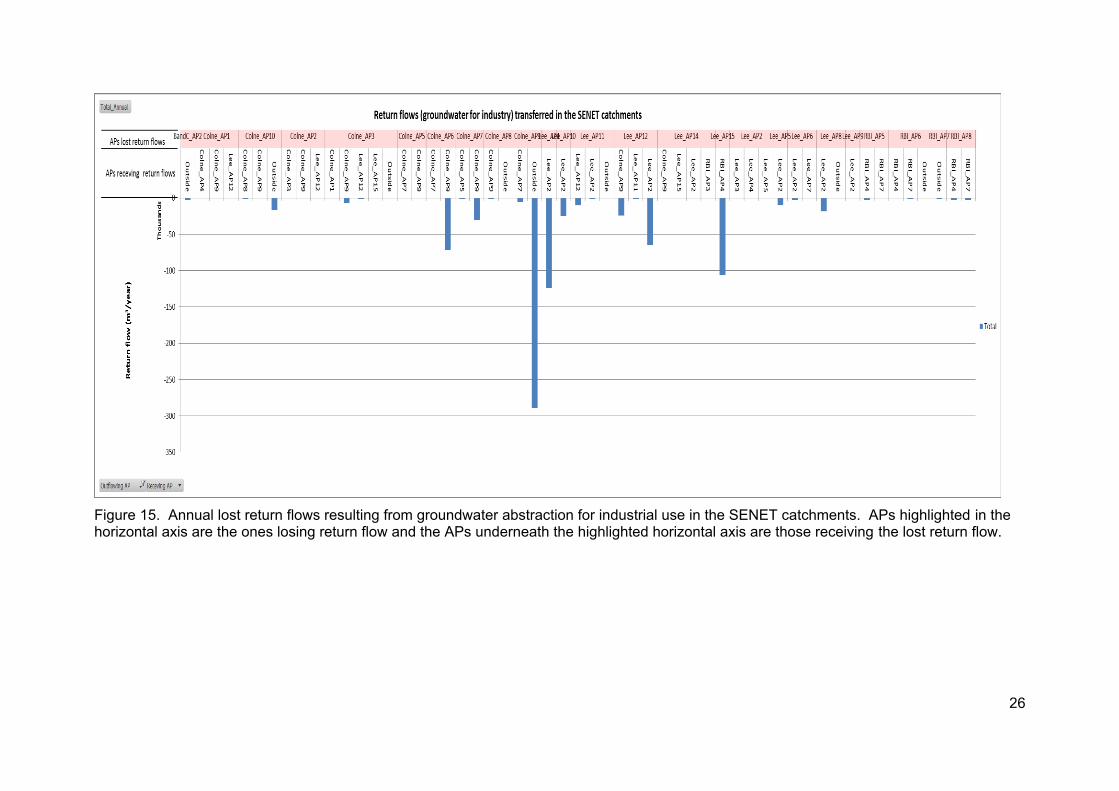
The analysis for the lost return flows resulting from groundwater abstraction used for industrial and domestic sectors is presented in Figure 15 and Figure 16. The total groundwater transferred to outside the SENET area after industrial use is 0.31 Mm3/year (STW Mogden). Ninety five percent of this return flow through STW Mogden is from or via Colne AP9. Colne AP9 also receives 0.14 Mm3/year of the return flows from other APs, such as Colne AP6, Colne AP7, Colne AP3 and Lee AP12.

23

Figure 11. Annual return flows resulting from surface water abstraction for industrial use in the SENET catchments. APs in the highlighted horizontal axis are the ones losing return flows (outflowing) and the APs underneath the highlighted horizontal axis are those receiving the lost return flows.

24

Figure 12. Monthly distribution of the lost return flows resulting from surface water abstraction for industrial sector. The APs labelled in the horizontal axis are the water receiving APs.

Figure 13. Annual return flows resulting from surface water abstraction for domestic use in the SENET catchments. APs highlighted in the horizontal axis are the ones losing return flow (outflowing) and the APs underneath the highlighted horizontal axis are those receiving the lost return flow.

25

Figure 14. Monthly distribution of the lost return flows resulting from surface water abstraction for domestic use. The APs labelled in the horizontal axis are the water receiving APs.

26

Figure 15. Annual lost return flows resulting from groundwater abstraction for industrial use in the SENET catchments. APs highlighted in the horizontal axis are the ones losing return flow and the APs underneath the highlighted horizontal axis are those receiving the lost return flow.

27

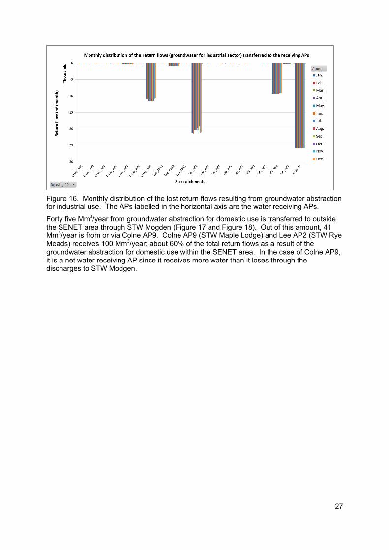
Figure 16. Monthly distribution of the lost return flows resulting from groundwater abstraction for industrial use. The APs labelled in the horizontal axis are the water receiving APs.

Forty five Mm3/year from groundwater abstraction for domestic use is transferred to outside the SENET area through STW Mogden (Figure 17 and Figure 18). Out of this amount, 41 Mm3/year is from or via Colne AP9. Colne AP9 (STW Maple Lodge) and Lee AP2 (STW Rye Meads) receives 100 Mm3/year; about 60% of the total return flows as a result of the groundwater abstraction for domestic use within the SENET area. In the case of Colne AP9, it is a net water receiving AP since it receives more water than it loses through the discharges to STW Modgen.

28

Figure 17. Annual lost return flows resulting from groundwater abstraction for domestic use in the SENET catchments. APs highlighted in the horizontal axis are the ones of lost return flow and the APs underneath the highlighted horizontal axis are those receiving the lost return flow.

29

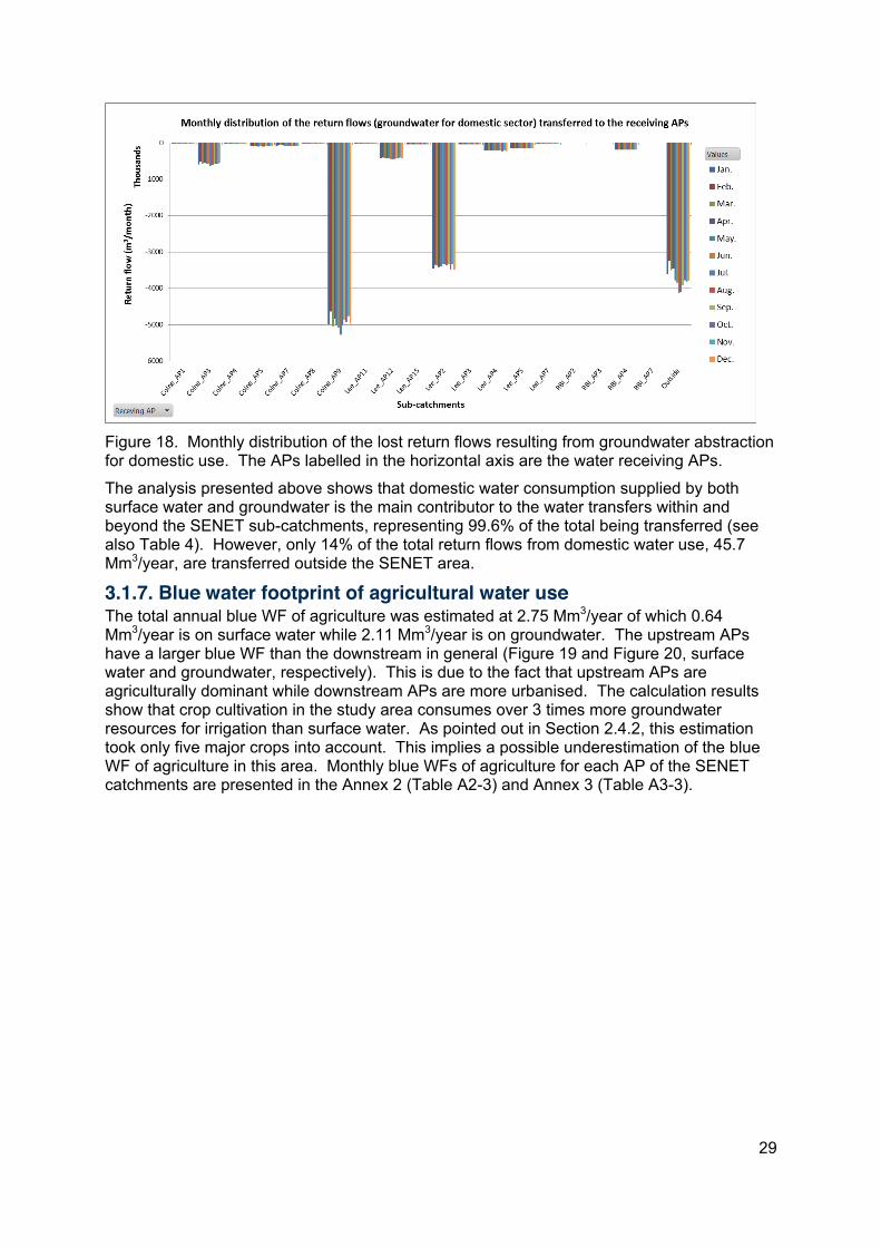
Figure 18. Monthly distribution of the lost return flows resulting from groundwater abstraction for domestic use. The APs labelled in the horizontal axis are the water receiving APs.

The analysis presented above shows that domestic water consumption supplied by both surface water and groundwater is the main contributor to the water transfers within and beyond the SENET sub-catchments, representing 99.6% of the total being transferred (see also Table 4). However, only 14% of the total return flows from domestic water use, 45.7 Mm3/year, are transferred outside the SENET area.

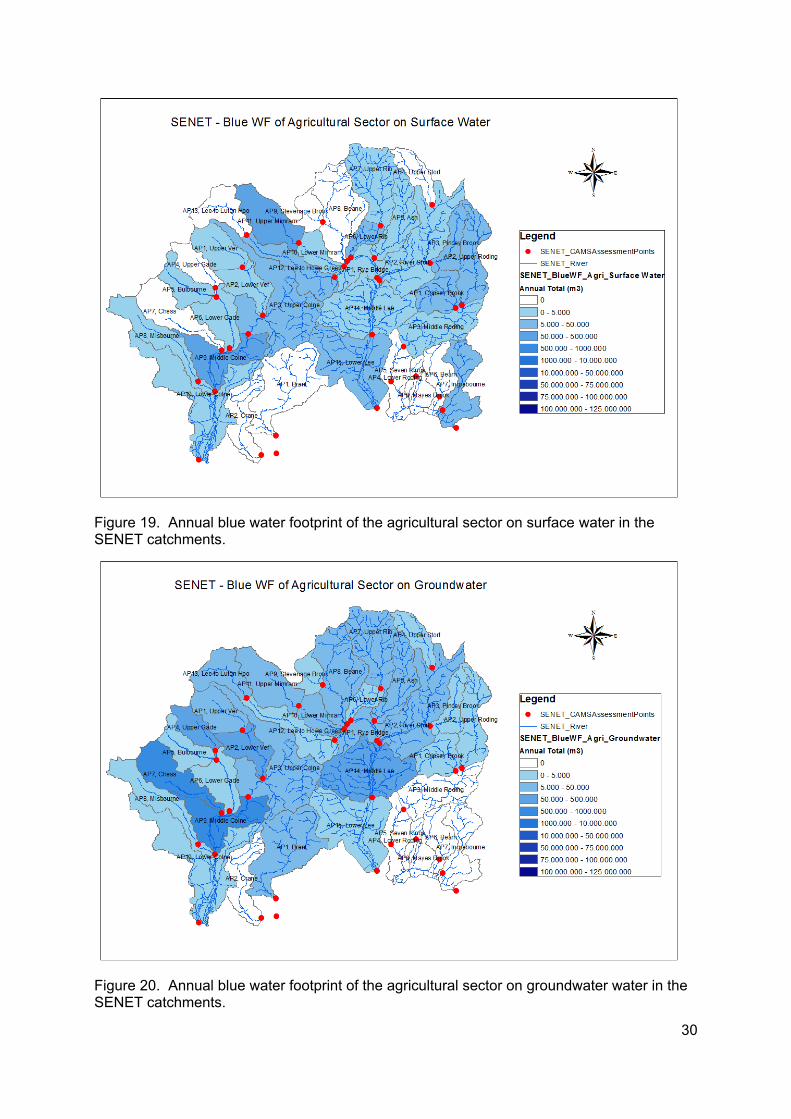
3.1.7. Blue water footprint of agricultural water use The total annual blue WF of agriculture was estimated at 2.75 Mm3/year of which 0.64 Mm3/year is on surface water while 2.11 Mm3/year is on groundwater. The upstream APs have a larger blue WF than the downstream in general (Figure 19 and Figure 20, surface water and groundwater, respectively). This is due to the fact that upstream APs are agriculturally dominant while downstream APs are more urbanised. The calculation results show that crop cultivation in the study area consumes over 3 times more groundwater resources for irrigation than surface water. As pointed out in Section 2.4.2, this estimation took only five major crops into account. This implies a possible underestimation of the blue WF of agriculture in this area. Monthly blue WFs of agriculture for each AP of the SENET catchments are presented in the Annex 2 (Table A2-3) and Annex 3 (Table A3-3).

30

Figure 19. Annual blue water footprint of the agricultural sector on surface water in the SENET catchments.

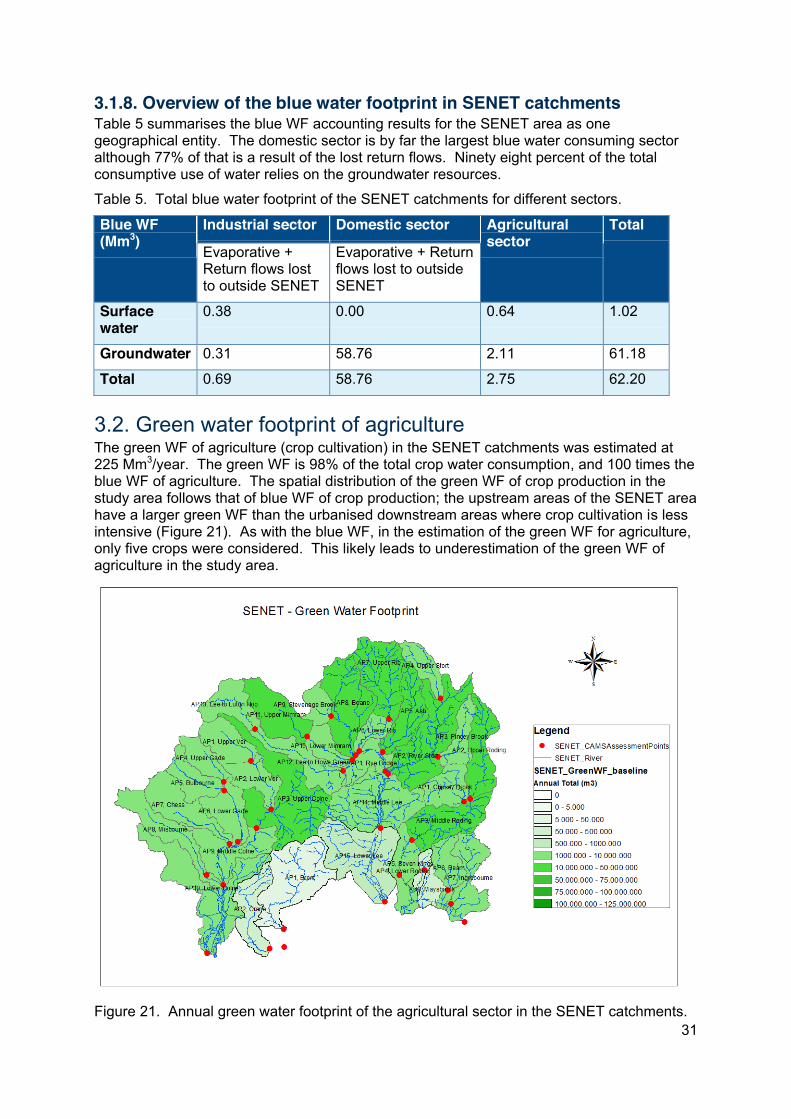
Figure 20. Annual blue water footprint of the agricultural sector on groundwater water in the SENET catchments.

31

3.1.8. Overview of the blue water footprint in SENET catchments Table 5 summarises the blue WF accounting results for the SENET area as one geographical entity. The domestic sector is by far the largest blue water consuming sector although 77% of that is a result of the lost return flows. Ninety eight percent of the total consumptive use of water relies on the groundwater resources.

Table 5. Total blue water footprint of the SENET catchments for different sectors.

Blue WF (Mm3)

Industrial sector Domestic sector Agricultural sector

Total

Evaporative + Return flows lost to outside SENET

Evaporative + Return flows lost to outside SENET

Surface water

0.38 0.00 0.64 1.02

Groundwater 0.31 58.76 2.11 61.18

Total 0.69 58.76 2.75 62.20

3.2. Green water footprint of agriculture The green WF of agriculture (crop cultivation) in the SENET catchments was estimated at 225 Mm3/year. The green WF is 98% of the total crop water consumption, and 100 times the blue WF of agriculture. The spatial distribution of the green WF of crop production in the study area follows that of blue WF of crop production; the upstream areas of the SENET area have a larger green WF than the urbanised downstream areas where crop cultivation is less intensive (Figure 21). As with the blue WF, in the estimation of the green WF for agriculture, only five crops were considered. This likely leads to underestimation of the green WF of agriculture in the study area.

Figure 21. Annual green water footprint of the agricultural sector in the SENET catchments.

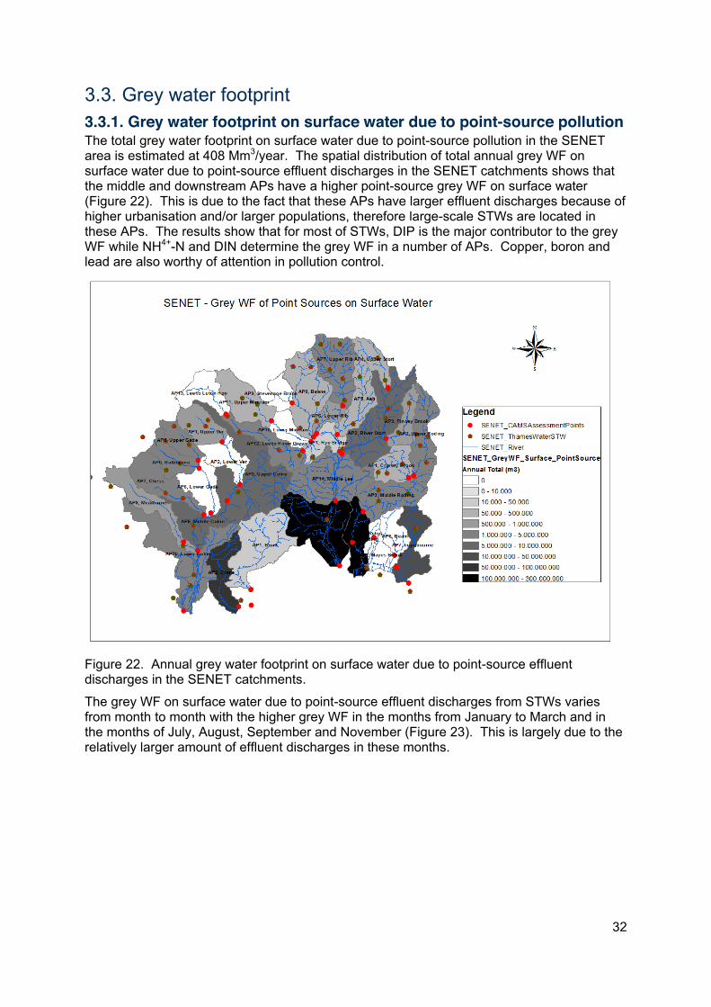
32

3.3. Grey water footprint 3.3.1. Grey water footprint on surface water due to point-source pollution The total grey water footprint on surface water due to point-source pollution in the SENET area is estimated at 408 Mm3/year. The spatial distribution of total annual grey WF on surface water due to point-source effluent discharges in the SENET catchments shows that the middle and downstream APs have a higher point-source grey WF on surface water (Figure 22). This is due to the fact that these APs have larger effluent discharges because of higher urbanisation and/or larger populations, therefore large-scale STWs are located in these APs. The results show that for most of STWs, DIP is the major contributor to the grey WF while NH4+-N and DIN determine the grey WF in a number of APs. Copper, boron and lead are also worthy of attention in pollution control.

Figure 22. Annual grey water footprint on surface water due to point-source effluent discharges in the SENET catchments.

The grey WF on surface water due to point-source effluent discharges from STWs varies from month to month with the higher grey WF in the months from January to March and in the months of July, August, September and November (Figure 23). This is largely due to the relatively larger amount of effluent discharges in these months.

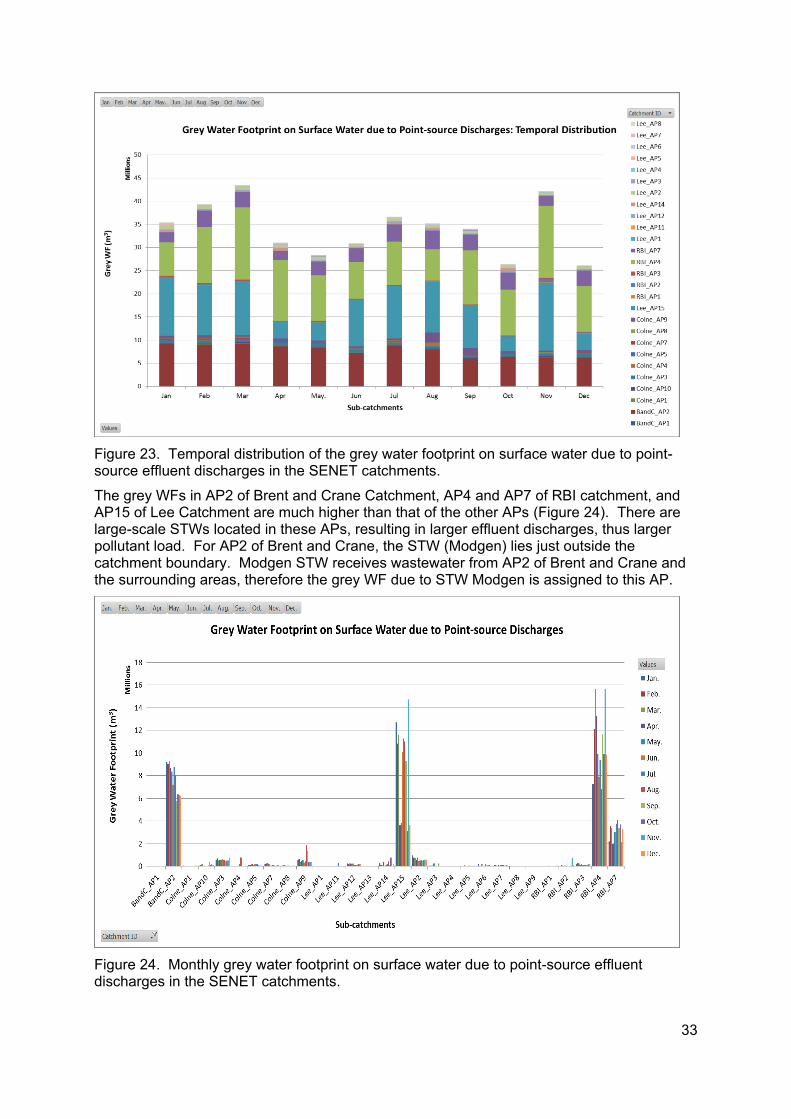
33

Figure 23. Temporal distribution of the grey water footprint on surface water due to point-source effluent discharges in the SENET catchments.

The grey WFs in AP2 of Brent and Crane Catchment, AP4 and AP7 of RBI catchment, and AP15 of Lee Catchment are much higher than that of the other APs (Figure 24). There are large-scale STWs located in these APs, resulting in larger effluent discharges, thus larger pollutant load. For AP2 of Brent and Crane, the STW (Modgen) lies just outside the catchment boundary. Modgen STW receives wastewater from AP2 of Brent and Crane and the surrounding areas, therefore the grey WF due to STW Modgen is assigned to this AP.

Figure 24. Monthly grey water footprint on surface water due to point-source effluent discharges in the SENET catchments.

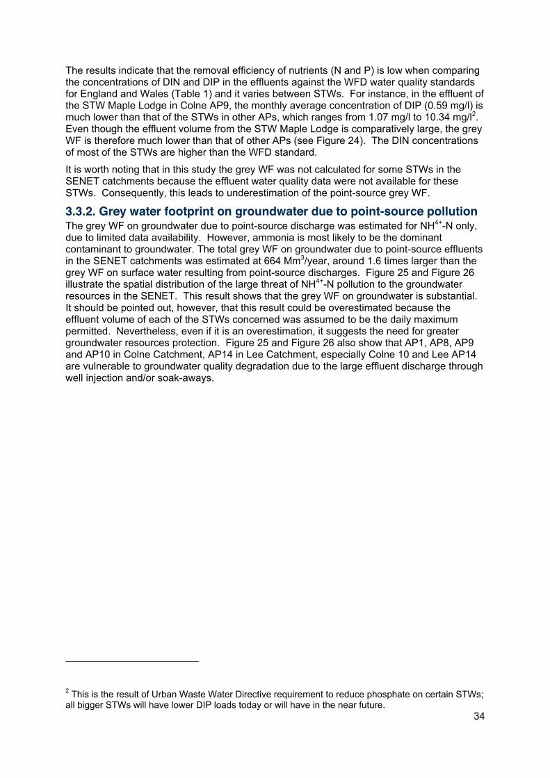
34

The results indicate that the removal efficiency of nutrients (N and P) is low when comparing the concentrations of DIN and DIP in the effluents against the WFD water quality standards for England and Wales (Table 1) and it varies between STWs. For instance, in the effluent of the STW Maple Lodge in Colne AP9, the monthly average concentration of DIP (0.59 mg/l) is much lower than that of the STWs in other APs, which ranges from 1.07 mg/l to 10.34 mg/l2. Even though the effluent volume from the STW Maple Lodge is comparatively large, the grey WF is therefore much lower than that of other APs (see Figure 24). The DIN concentrations of most of the STWs are higher than the WFD standard.

It is worth noting that in this study the grey WF was not calculated for some STWs in the SENET catchments because the effluent water quality data were not available for these STWs. Consequently, this leads to underestimation of the point-source grey WF.

3.3.2. Grey water footprint on groundwater due to point-source pollution The grey WF on groundwater due to point-source discharge was estimated for NH4+-N only, due to limited data availability. However, ammonia is most likely to be the dominant contaminant to groundwater. The total grey WF on groundwater due to point-source effluents in the SENET catchments was estimated at 664 Mm3/year, around 1.6 times larger than the grey WF on surface water resulting from point-source discharges. Figure 25 and Figure 26 illustrate the spatial distribution of the large threat of NH4+-N pollution to the groundwater resources in the SENET. This result shows that the grey WF on groundwater is substantial. It should be pointed out, however, that this result could be overestimated because the effluent volume of each of the STWs concerned was assumed to be the daily maximum permitted. Nevertheless, even if it is an overestimation, it suggests the need for greater groundwater resources protection. Figure 25 and Figure 26 also show that AP1, AP8, AP9 and AP10 in Colne Catchment, AP14 in Lee Catchment, especially Colne 10 and Lee AP14 are vulnerable to groundwater quality degradation due to the large effluent discharge through well injection and/or soak-aways.

2 This is the result of Urban Waste Water Directive requirement to reduce phosphate on certain STWs; all bigger STWs will have lower DIP loads today or will have in the near future.

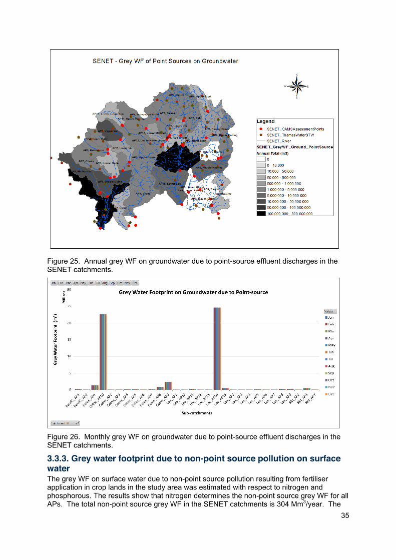
35

Figure 25. Annual grey WF on groundwater due to point-source effluent discharges in the SENET catchments.

Figure 26. Monthly grey WF on groundwater due to point-source effluent discharges in the SENET catchments.

3.3.3. Grey water footprint due to non-point source pollution on surface water The grey WF on surface water due to non-point source pollution resulting from fertiliser application in crop lands in the study area was estimated with respect to nitrogen and phosphorous. The results show that nitrogen determines the non-point source grey WF for all APs. The total non-point source grey WF in the SENET catchments is 304 Mm3/year. The

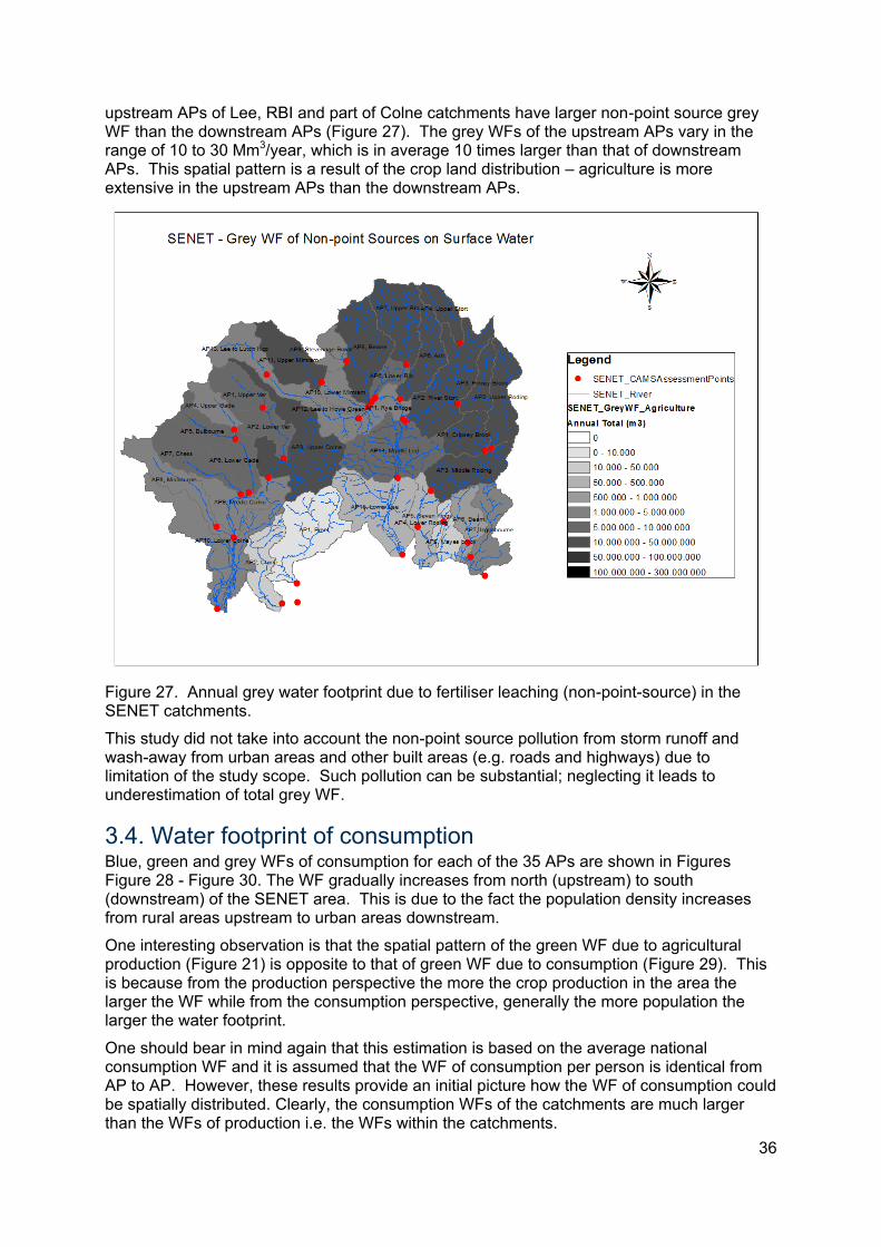
36

upstream APs of Lee, RBI and part of Colne catchments have larger non-point source grey WF than the downstream APs (Figure 27). The grey WFs of the upstream APs vary in the range of 10 to 30 Mm3/year, which is in average 10 times larger than that of downstream APs. This spatial pattern is a result of the crop land distribution – agriculture is more extensive in the upstream APs than the downstream APs.

Figure 27. Annual grey water footprint due to fertiliser leaching (non-point-source) in the SENET catchments.

This study did not take into account the non-point source pollution from storm runoff and wash-away from urban areas and other built areas (e.g. roads and highways) due to limitation of the study scope. Such pollution can be substantial; neglecting it leads to underestimation of total grey WF.

3.4. Water footprint of consumption Blue, green and grey WFs of consumption for each of the 35 APs are shown in Figures Figure 28 - Figure 30. The WF gradually increases from north (upstream) to south (downstream) of the SENET area. This is due to the fact the population density increases from rural areas upstream to urban areas downstream.

One interesting observation is that the spatial pattern of the green WF due to agricultural production (Figure 21) is opposite to that of green WF due to consumption (Figure 29). This is because from the production perspective the more the crop production in the area the larger the WF while from the consumption perspective, generally the more population the larger the water footprint.

One should bear in mind again that this estimation is based on the average national consumption WF and it is assumed that the WF of consumption per person is identical from AP to AP. However, these results provide an initial picture how the WF of consumption could be spatially distributed. Clearly, the consumption WFs of the catchments are much larger than the WFs of production i.e. the WFs within the catchments.

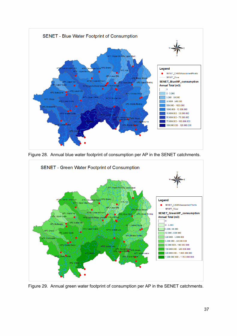
37

Figure 28. Annual blue water footprint of consumption per AP in the SENET catchments.

Figure 29. Annual green water footprint of consumption per AP in the SENET catchments.

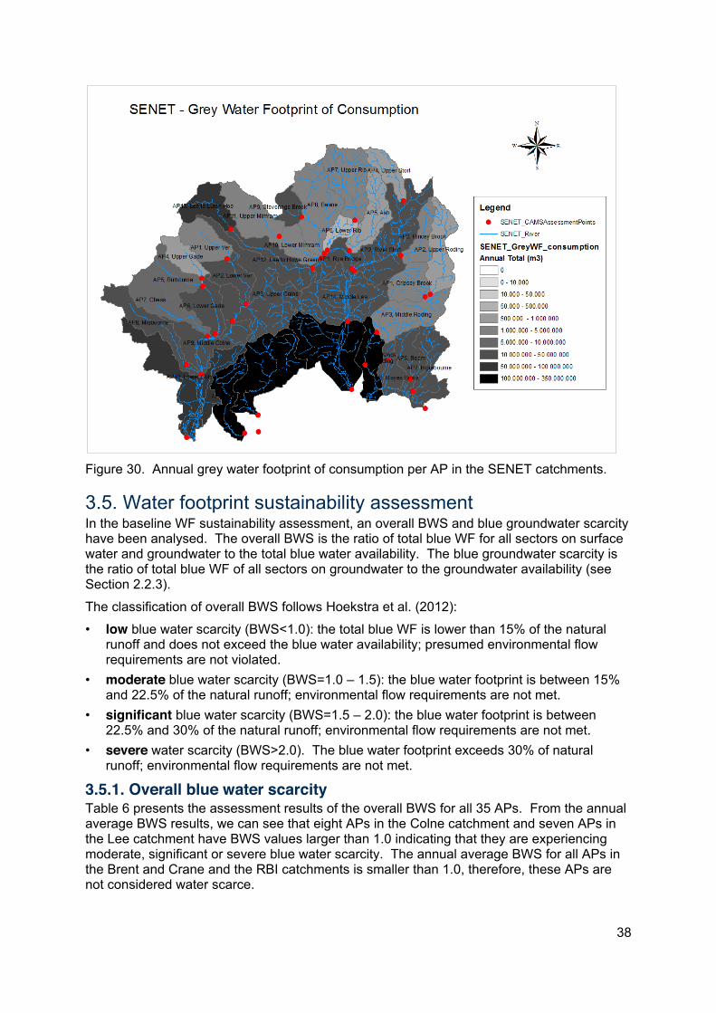
38

Figure 30. Annual grey water footprint of consumption per AP in the SENET catchments.

3.5. Water footprint sustainability assessment In the baseline WF sustainability assessment, an overall BWS and blue groundwater scarcity have been analysed. The overall BWS is the ratio of total blue WF for all sectors on surface water and groundwater to the total blue water availability. The blue groundwater scarcity is the ratio of total blue WF of all sectors on groundwater to the groundwater availability (see Section 2.2.3).

The classification of overall BWS follows Hoekstra et al. (2012):

• low blue water scarcity (BWS<1.0): the total blue WF is lower than 15% of the natural runoff and does not exceed the blue water availability; presumed environmental flow requirements are not violated.

• moderate blue water scarcity (BWS=1.0 – 1.5): the blue water footprint is between 15% and 22.5% of the natural runoff; environmental flow requirements are not met.

• significant blue water scarcity (BWS=1.5 – 2.0): the blue water footprint is between 22.5% and 30% of the natural runoff; environmental flow requirements are not met.

• severe water scarcity (BWS>2.0). The blue water footprint exceeds 30% of natural runoff; environmental flow requirements are not met.

3.5.1. Overall blue water scarcity Table 6 presents the assessment results of the overall BWS for all 35 APs. From the annual average BWS results, we can see that eight APs in the Colne catchment and seven APs in the Lee catchment have BWS values larger than 1.0 indicating that they are experiencing moderate, significant or severe blue water scarcity. The annual average BWS for all APs in the Brent and Crane and the RBI catchments is smaller than 1.0, therefore, these APs are not considered water scarce.

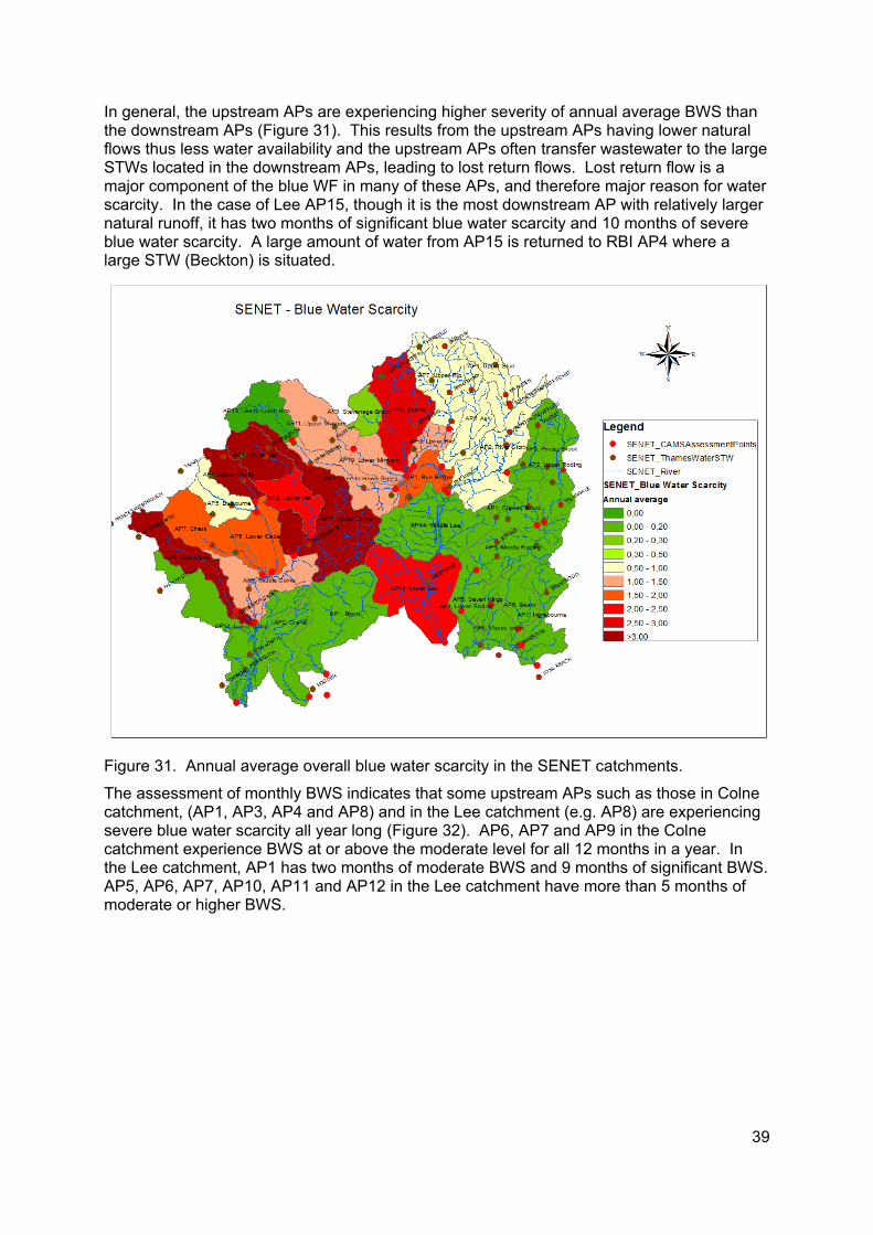
39

In general, the upstream APs are experiencing higher severity of annual average BWS than the downstream APs (Figure 31). This results from the upstream APs having lower natural flows thus less water availability and the upstream APs often transfer wastewater to the large STWs located in the downstream APs, leading to lost return flows. Lost return flow is a major component of the blue WF in many of these APs, and therefore major reason for water scarcity. In the case of Lee AP15, though it is the most downstream AP with relatively larger natural runoff, it has two months of significant blue water scarcity and 10 months of severe blue water scarcity. A large amount of water from AP15 is returned to RBI AP4 where a large STW (Beckton) is situated.

Figure 31. Annual average overall blue water scarcity in the SENET catchments.

The assessment of monthly BWS indicates that some upstream APs such as those in Colne catchment, (AP1, AP3, AP4 and AP8) and in the Lee catchment (e.g. AP8) are experiencing severe blue water scarcity all year long (Figure 32). AP6, AP7 and AP9 in the Colne catchment experience BWS at or above the moderate level for all 12 months in a year. In the Lee catchment, AP1 has two months of moderate BWS and 9 months of significant BWS. AP5, AP6, AP7, AP10, AP11 and AP12 in the Lee catchment have more than 5 months of moderate or higher BWS.

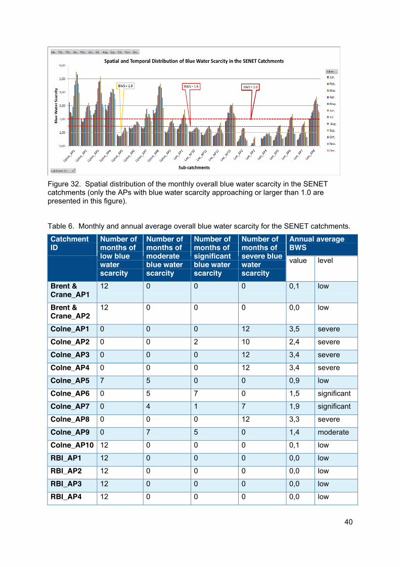
40

Figure 32. Spatial distribution of the monthly overall blue water scarcity in the SENET catchments (only the APs with blue water scarcity approaching or larger than 1.0 are presented in this figure).

Table 6. Monthly and annual average overall blue water scarcity for the SENET catchments.

Catchment ID

Number of months of low blue water scarcity

Number of months of moderate blue water scarcity

Number of months of significant blue water scarcity

Number of months of severe blue water scarcity

Annual average BWS value level

Brent & Crane_AP1

12 0 0 0 0,1 low

Brent & Crane_AP2

12 0 0 0 0,0 low

Colne_AP1 0 0 0 12 3,5 severe

Colne_AP2 0 0 2 10 2,4 severe

Colne_AP3 0 0 0 12 3,4 severe

Colne_AP4 0 0 0 12 3,4 severe

Colne_AP5 7 5 0 0 0,9 low

Colne_AP6 0 5 7 0 1,5 significant

Colne_AP7 0 4 1 7 1,9 significant

Colne_AP8 0 0 0 12 3,3 severe

Colne_AP9 0 7 5 0 1,4 moderate

Colne_AP10 12 0 0 0 0,1 low

RBI_AP1 12 0 0 0 0,0 low

RBI_AP2 12 0 0 0 0,0 low

RBI_AP3 12 0 0 0 0,0 low

RBI_AP4 12 0 0 0 0,0 low

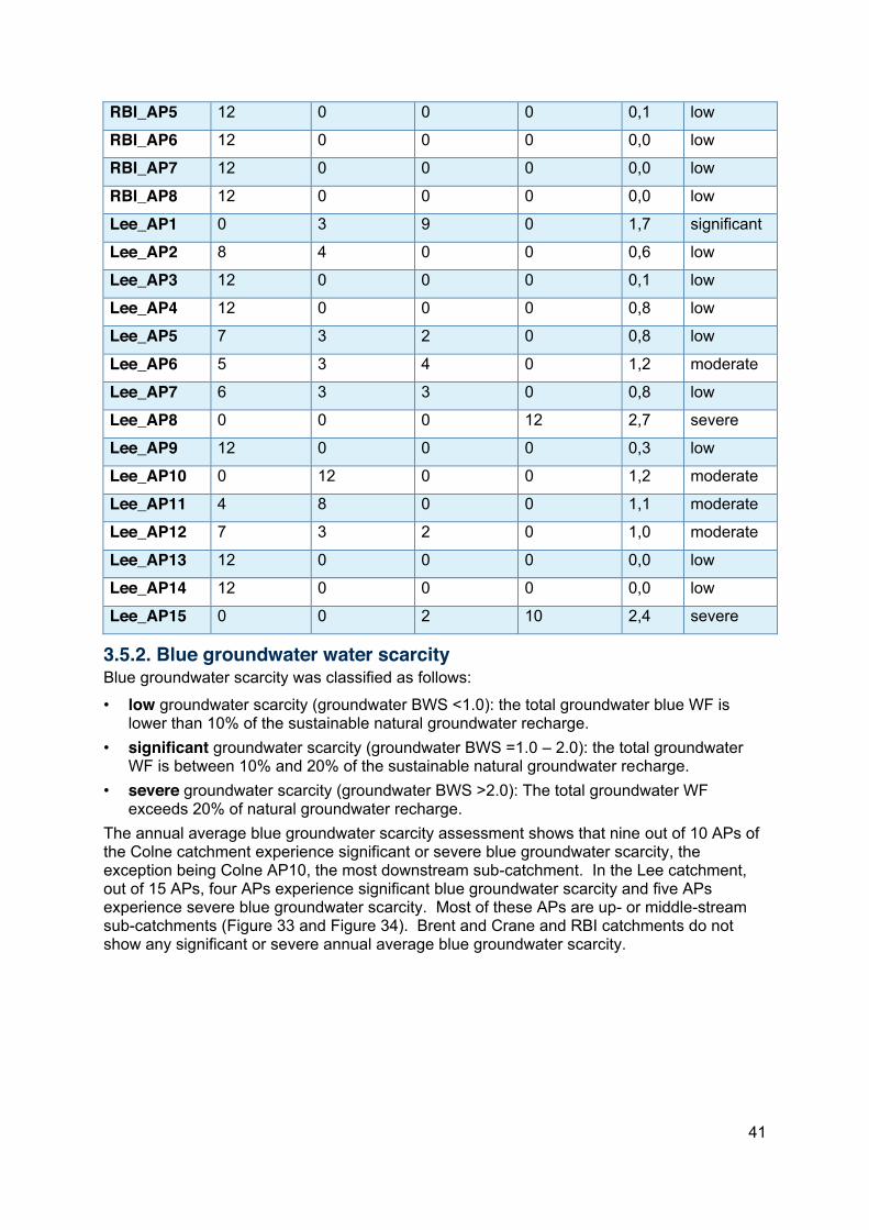
41

RBI_AP5 12 0 0 0 0,1 low

RBI_AP6 12 0 0 0 0,0 low

RBI_AP7 12 0 0 0 0,0 low

RBI_AP8 12 0 0 0 0,0 low

Lee_AP1 0 3 9 0 1,7 significant

Lee_AP2 8 4 0 0 0,6 low

Lee_AP3 12 0 0 0 0,1 low

Lee_AP4 12 0 0 0 0,8 low

Lee_AP5 7 3 2 0 0,8 low

Lee_AP6 5 3 4 0 1,2 moderate

Lee_AP7 6 3 3 0 0,8 low

Lee_AP8 0 0 0 12 2,7 severe

Lee_AP9 12 0 0 0 0,3 low

Lee_AP10 0 12 0 0 1,2 moderate

Lee_AP11 4 8 0 0 1,1 moderate

Lee_AP12 7 3 2 0 1,0 moderate

Lee_AP13 12 0 0 0 0,0 low

Lee_AP14 12 0 0 0 0,0 low

Lee_AP15 0 0 2 10 2,4 severe

3.5.2. Blue groundwater water scarcity Blue groundwater scarcity was classified as follows:

• low groundwater scarcity (groundwater BWS <1.0): the total groundwater blue WF is lower than 10% of the sustainable natural groundwater recharge.

• significant groundwater scarcity (groundwater BWS =1.0 – 2.0): the total groundwater WF is between 10% and 20% of the sustainable natural groundwater recharge.

• severe groundwater scarcity (groundwater BWS >2.0): The total groundwater WF exceeds 20% of natural groundwater recharge.

The annual average blue groundwater scarcity assessment shows that nine out of 10 APs of the Colne catchment experience significant or severe blue groundwater scarcity, the exception being Colne AP10, the most downstream sub-catchment. In the Lee catchment, out of 15 APs, four APs experience significant blue groundwater scarcity and five APs experience severe blue groundwater scarcity. Most of these APs are up- or middle-stream sub-catchments (Figure 33 and Figure 34). Brent and Crane and RBI catchments do not show any significant or severe annual average blue groundwater scarcity.

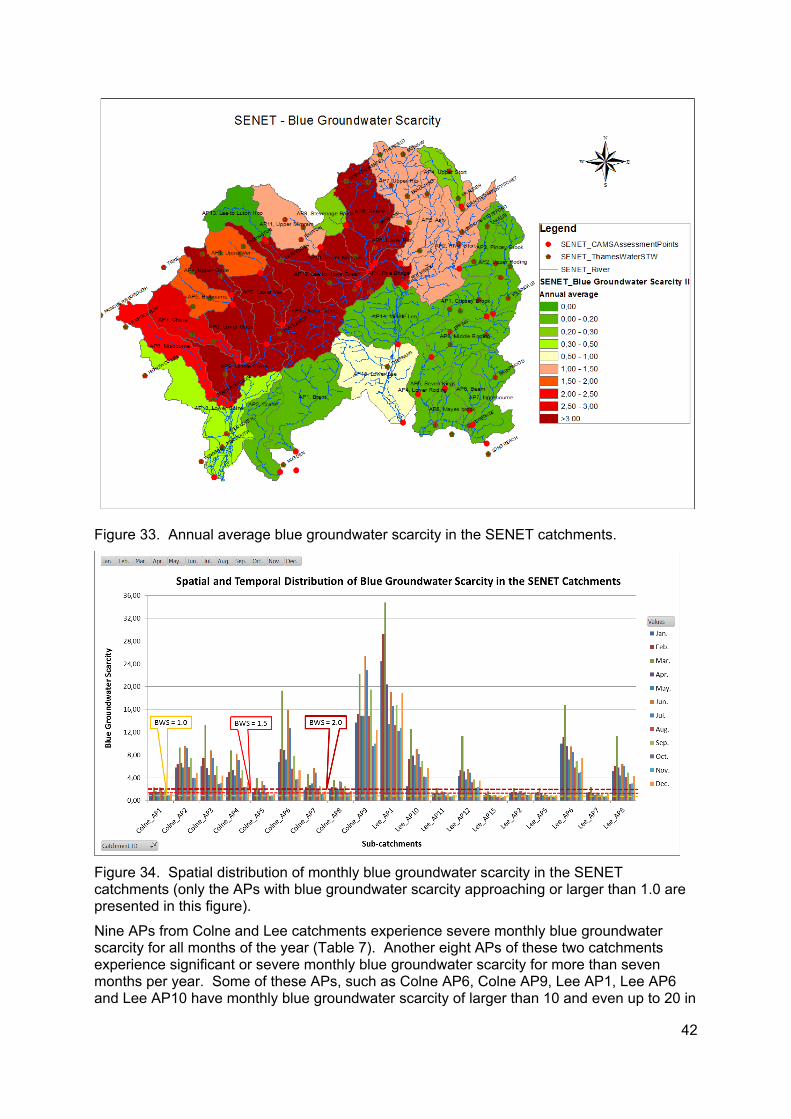
42

Figure 33. Annual average blue groundwater scarcity in the SENET catchments.

Figure 34. Spatial distribution of monthly blue groundwater scarcity in the SENET catchments (only the APs with blue groundwater scarcity approaching or larger than 1.0 are presented in this figure).

Nine APs from Colne and Lee catchments experience severe monthly blue groundwater scarcity for all months of the year (Table 7). Another eight APs of these two catchments experience significant or severe monthly blue groundwater scarcity for more than seven months per year. Some of these APs, such as Colne AP6, Colne AP9, Lee AP1, Lee AP6 and Lee AP10 have monthly blue groundwater scarcity of larger than 10 and even up to 20 in

43

many months indicating that sustainable natural recharge has been violated by 100% -200%, namely the sustainable recharge has been fully consumed and the groundwater reserve has been overabstracted. The most severe groundwater scarcity, with a BWS value of 35, occurs in March in Lee AP1. Groundwater is the major source for all three sectors in the study area and the groundwater abstracted in many APs is not returned to the original source. For example, about 40 Mm3/year of groundwater abstracted from Colne AP9 is transferred to outside the SENET area, leading to high blue groundwater scarcity in this AP. In the case Lee AP1, more than 80% of its blue WF on groundwater results from the lost return flows while the natural recharge of this AP is less than the average natural recharge in the study area, giving rise to very high groundwater scarcity. Detailed monthly groundwater BWS results are presented in Table A7-2 of Annex 7.

Table 7. Monthly and annual average blue groundwater scarcity for the SENET catchments.

Catchment ID

Number of months of low groundwater BWS

Number of months of significant groundwater BWS

Number of months of severe groundwater BWS

Annual average groundwater BWS value level

Brent & Crane_AP1

12 0 0 0,0 low

Brent & Crane_AP2

12 0 0 0,0 low

Colne_AP1 2 7 3 1,6 significant

Colne_AP2 0 0 12 6,6 severe

Colne_AP3 0 0 12 6,2 severe

Colne_AP4 0 0 12 5,0 severe

Colne_AP5 2 7 3 1,9 significant

Colne_AP6 0 0 12 8,8 severe

Colne_AP7 0 5 7 2,8 severe

Colne_AP8 0 3 9 2,3 severe

Colne_AP9 0 0 12 16,3 severe

Colne_AP10 12 0 0 0,4 low

RBI_AP1 12 0 0 0,0 low

RBI_AP2 12 0 0 0,0 low

RBI_AP3 12 0 0 0,0 low

RBI_AP4 12 0 0 0,0 low

RBI_AP5 12 0 0 0,1 low

RBI_AP6 12 0 0 0,0 low

RBI_AP7 12 0 0 0,0 low

RBI_AP8 12 0 0 0,0 low

Lee_AP1 0 0 12 19,3 severe

Lee_AP2 1 10 1 1,4 significant

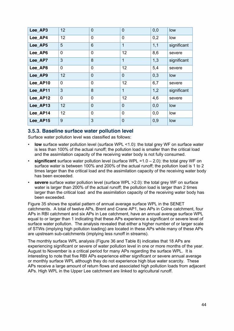
44

Lee_AP3 12 0 0 0,0 low

Lee_AP4 12 0 0 0,2 low

Lee_AP5 5 6 1 1,1 significant

Lee_AP6 0 0 12 8,6 severe

Lee_AP7 3 8 1 1,3 significant

Lee_AP8 0 0 12 5,4 severe

Lee_AP9 12 0 0 0,3 low

Lee_AP10 0 0 12 6,7 severe

Lee_AP11 3 8 1 1,2 significant

Lee_AP12 0 0 12 4,6 severe

Lee_AP13 12 0 0 0,0 low

Lee_AP14 12 0 0 0,0 low

Lee_AP15 9 3 0 0,9 low

3.5.3. Baseline surface water pollution level Surface water pollution level was classified as follows:

• low surface water pollution level (surface WPL <1.0): the total grey WF on surface water is less than 100% of the actual runoff; the pollution load is smaller than the critical load and the assimilation capacity of the receiving water body is not fully consumed.

• significant surface water pollution level (surface WPL =1.0 – 2.0): the total grey WF on surface water is between 100% and 200% of the actual runoff; the pollution load is 1 to 2 times larger than the critical load and the assimilation capacity of the receiving water body has been exceeded.

• severe surface water pollution level (surface WPL >2.0): the total grey WF on surface water is larger than 200% of the actual runoff; the pollution load is larger than 2 times larger than the critical load and the assimilation capacity of the receiving water body has been exceeded.

Figure 35 shows the spatial pattern of annual average surface WPL in the SENET catchments. A total of twelve APs, Brent and Crane AP1, two APs in Colne catchment, four APs in RBI catchment and six APs in Lee catchment, have an annual average surface WPL equal to or larger than 1 indicating that these APs experience a significant or severe level of surface water pollution. The analysis revealed that either a higher number of or larger scale of STWs (implying high pollution loading) are located in these APs while many of these APs are upstream sub-catchments (implying less runoff in streams).

The monthly surface WPL analysis (Figure 36 and Table 8) indicates that 18 APs are experiencing significant or severe of water pollution level in one or more months of the year. August to November is a critical period for many APs regarding the surface WPL. It is interesting to note that five RBI APs experience either significant or severe annual average or monthly surface WPL although they do not experience high blue water scarcity. These APs receive a large amount of return flows and associated high pollution loads from adjacent APs. High WPL in the Upper Lee catchment are linked to agricultural runoff.

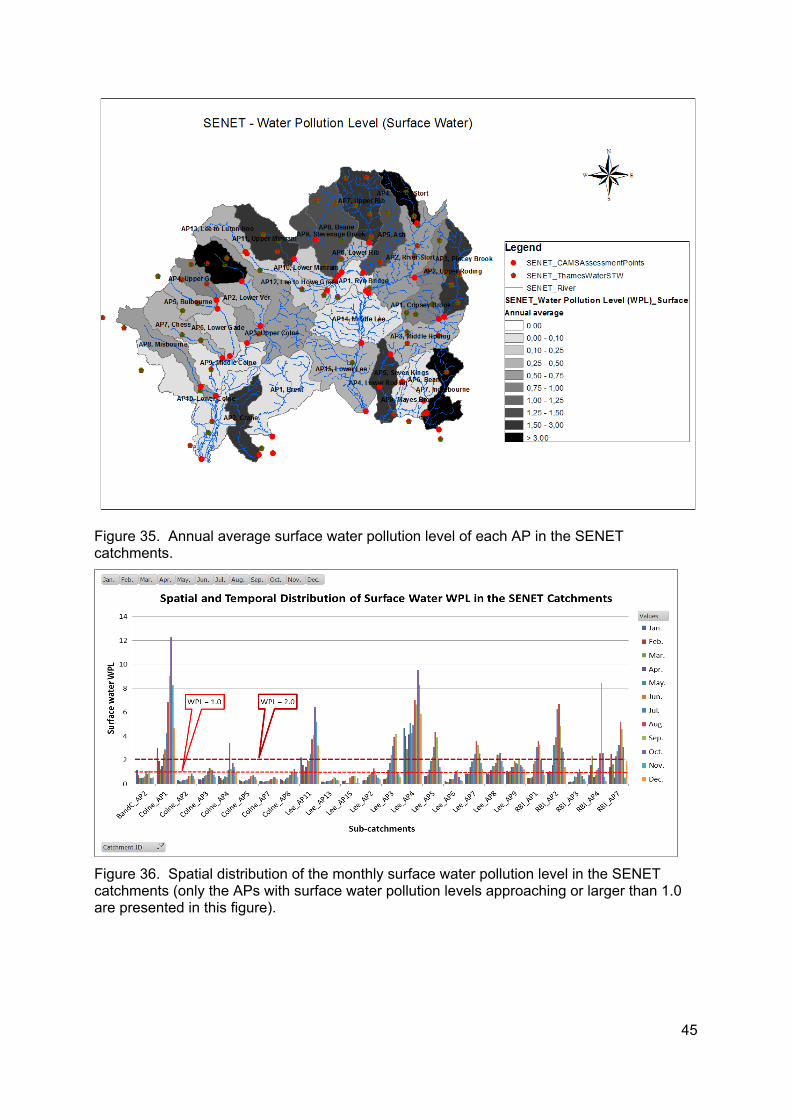
45

Figure 35. Annual average surface water pollution level of each AP in the SENET catchments.

Figure 36. Spatial distribution of the monthly surface water pollution level in the SENET catchments (only the APs with surface water pollution levels approaching or larger than 1.0 are presented in this figure).

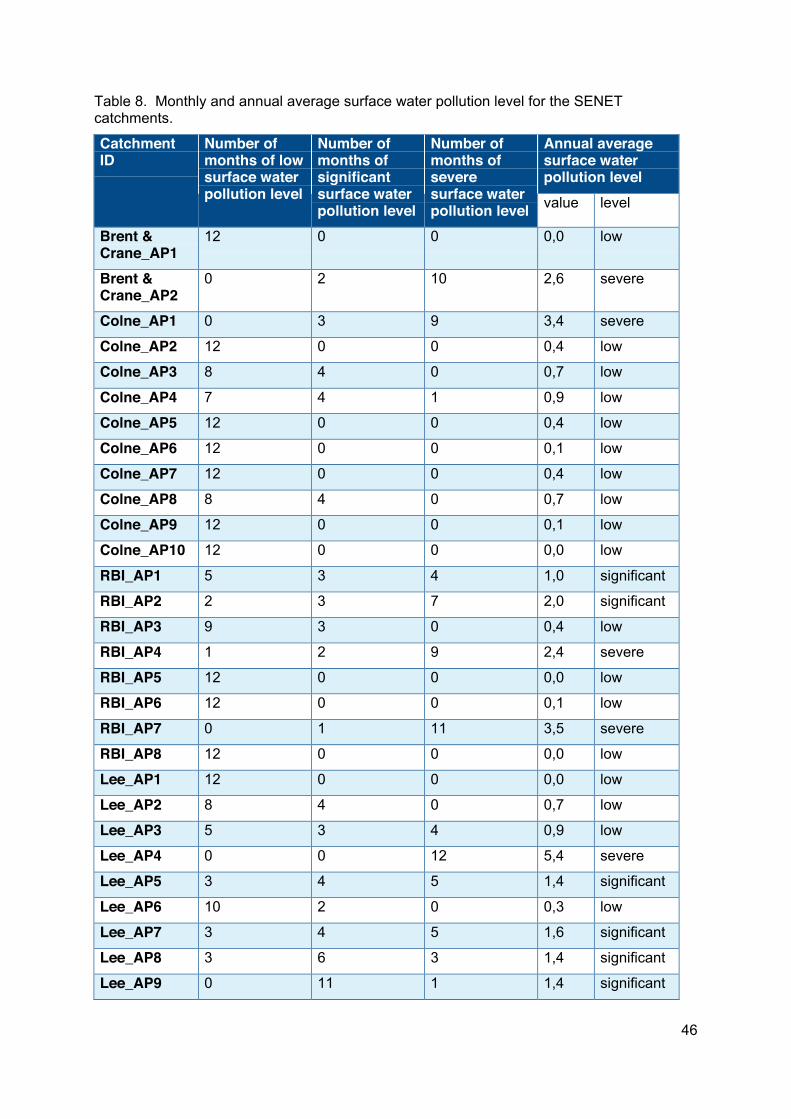
46

Table 8. Monthly and annual average surface water pollution level for the SENET catchments.

Catchment ID

Number of months of low surface water pollution level

Number of months of significant surface water pollution level

Number of months of severe surface water pollution level

Annual average surface water pollution level value level

Brent & Crane_AP1

12 0 0 0,0 low

Brent & Crane_AP2

0 2 10 2,6 severe

Colne_AP1 0 3 9 3,4 severe

Colne_AP2 12 0 0 0,4 low

Colne_AP3 8 4 0 0,7 low

Colne_AP4 7 4 1 0,9 low

Colne_AP5 12 0 0 0,4 low

Colne_AP6 12 0 0 0,1 low

Colne_AP7 12 0 0 0,4 low

Colne_AP8 8 4 0 0,7 low

Colne_AP9 12 0 0 0,1 low

Colne_AP10 12 0 0 0,0 low

RBI_AP1 5 3 4 1,0 significant

RBI_AP2 2 3 7 2,0 significant

RBI_AP3 9 3 0 0,4 low

RBI_AP4 1 2 9 2,4 severe

RBI_AP5 12 0 0 0,0 low

RBI_AP6 12 0 0 0,1 low

RBI_AP7 0 1 11 3,5 severe

RBI_AP8 12 0 0 0,0 low

Lee_AP1 12 0 0 0,0 low

Lee_AP2 8 4 0 0,7 low

Lee_AP3 5 3 4 0,9 low

Lee_AP4 0 0 12 5,4 severe

Lee_AP5 3 4 5 1,4 significant

Lee_AP6 10 2 0 0,3 low

Lee_AP7 3 4 5 1,6 significant

Lee_AP8 3 6 3 1,4 significant

Lee_AP9 0 11 1 1,4 significant

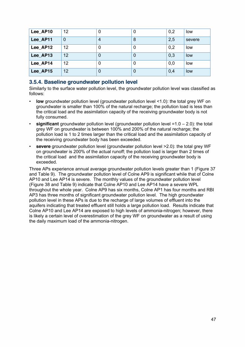
47

Lee_AP10 12 0 0 0,2 low

Lee_AP11 0 4 8 2,5 severe

Lee_AP12 12 0 0 0,2 low

Lee_AP13 12 0 0 0,3 low

Lee_AP14 12 0 0 0,0 low

Lee_AP15 12 0 0 0,4 low

3.5.4. Baseline groundwater pollution level Similarly to the surface water pollution level, the groundwater pollution level was classified as follows:

• low groundwater pollution level (groundwater pollution level <1.0): the total grey WF on groundwater is smaller than 100% of the natural recharge; the pollution load is less than the critical load and the assimilation capacity of the receiving groundwater body is not fully consumed.

• significant groundwater pollution level (groundwater pollution level =1.0 – 2.0): the total grey WF on groundwater is between 100% and 200% of the natural recharge; the pollution load is 1 to 2 times larger than the critical load and the assimilation capacity of the receiving groundwater body has been exceeded.

• severe groundwater pollution level (groundwater pollution level >2.0): the total grey WF on groundwater is 200% of the actual runoff; the pollution load is larger than 2 times of the critical load and the assimilation capacity of the receiving groundwater body is exceeded.

Three APs experience annual average groundwater pollution levels greater than 1 (Figure 37 and Table 9). The groundwater pollution level of Colne AP9 is significant while that of Colne AP10 and Lee AP14 is severe. The monthly values of the groundwater pollution level (Figure 38 and Table 9) indicate that Colne AP10 and Lee AP14 have a severe WPL throughout the whole year. Colne AP9 has six months, Colne AP1 has four months and RBI AP3 has three months of significant groundwater pollution level. The high groundwater pollution level in these APs is due to the recharge of large volumes of effluent into the aquifers indicating that treated effluent still holds a large pollution load. Results indicate that Colne AP10 and Lee AP14 are exposed to high levels of ammonia-nitrogen; however, there is likely a certain level of overestimation of the grey WF on groundwater as a result of using the daily maximum load of the ammonia-nitrogen.

48

Figure 37. Annual average groundwater pollution level of the SENET catchments.

Figure 38. Spatial distribution of the monthly groundwater pollution level in the SENET catchments (only the APs with groundwater pollution level approaching or larger than 1.0 are presented in this figure).

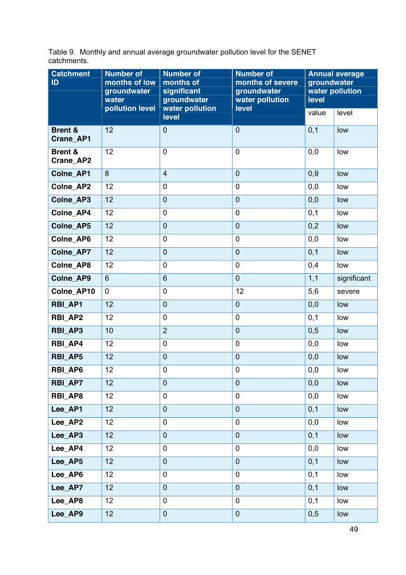
49

Table 9. Monthly and annual average groundwater pollution level for the SENET catchments.

Catchment ID

Number of months of low groundwater water pollution level

Number of months of significant groundwater water pollution level

Number of months of severe groundwater water pollution level

Annual average groundwater water pollution level value level

Brent & Crane_AP1

12 0 0 0,1 low

Brent & Crane_AP2

12 0 0 0,0 low

Colne_AP1 8 4 0 0,9 low

Colne_AP2 12 0 0 0,0 low

Colne_AP3 12 0 0 0,0 low

Colne_AP4 12 0 0 0,1 low

Colne_AP5 12 0 0 0,2 low

Colne_AP6 12 0 0 0,0 low

Colne_AP7 12 0 0 0,1 low

Colne_AP8 12 0 0 0,4 low

Colne_AP9 6 6 0 1,1 significant

Colne_AP10 0 0 12 5,6 severe

RBI_AP1 12 0 0 0,0 low

RBI_AP2 12 0 0 0,1 low

RBI_AP3 10 2 0 0,5 low

RBI_AP4 12 0 0 0,0 low

RBI_AP5 12 0 0 0,0 low

RBI_AP6 12 0 0 0,0 low

RBI_AP7 12 0 0 0,0 low

RBI_AP8 12 0 0 0,0 low

Lee_AP1 12 0 0 0,1 low

Lee_AP2 12 0 0 0,0 low

Lee_AP3 12 0 0 0,1 low

Lee_AP4 12 0 0 0,0 low

Lee_AP5 12 0 0 0,1 low

Lee_AP6 12 0 0 0,1 low

Lee_AP7 12 0 0 0,1 low

Lee_AP8 12 0 0 0,1 low

Lee_AP9 12 0 0 0,5 low

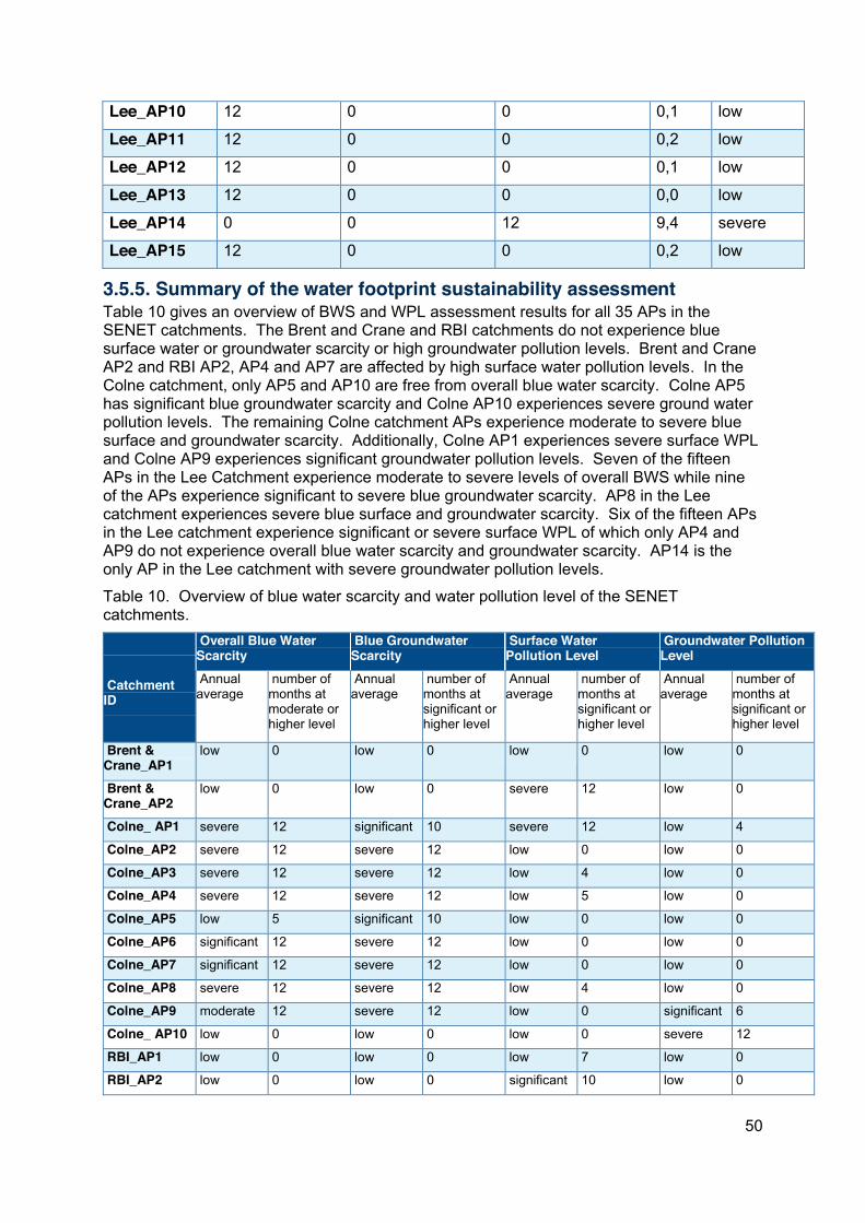
50

Lee_AP10 12 0 0 0,1 low

Lee_AP11 12 0 0 0,2 low

Lee_AP12 12 0 0 0,1 low

Lee_AP13 12 0 0 0,0 low

Lee_AP14 0 0 12 9,4 severe

Lee_AP15 12 0 0 0,2 low

3.5.5. Summary of the water footprint sustainability assessment Table 10 gives an overview of BWS and WPL assessment results for all 35 APs in the SENET catchments. The Brent and Crane and RBI catchments do not experience blue surface water or groundwater scarcity or high groundwater pollution levels. Brent and Crane AP2 and RBI AP2, AP4 and AP7 are affected by high surface water pollution levels. In the Colne catchment, only AP5 and AP10 are free from overall blue water scarcity. Colne AP5 has significant blue groundwater scarcity and Colne AP10 experiences severe ground water pollution levels. The remaining Colne catchment APs experience moderate to severe blue surface and groundwater scarcity. Additionally, Colne AP1 experiences severe surface WPL and Colne AP9 experiences significant groundwater pollution levels. Seven of the fifteen APs in the Lee Catchment experience moderate to severe levels of overall BWS while nine of the APs experience significant to severe blue groundwater scarcity. AP8 in the Lee catchment experiences severe blue surface and groundwater scarcity. Six of the fifteen APs in the Lee catchment experience significant or severe surface WPL of which only AP4 and AP9 do not experience overall blue water scarcity and groundwater scarcity. AP14 is the only AP in the Lee catchment with severe groundwater pollution levels.

Table 10. Overview of blue water scarcity and water pollution level of the SENET catchments.

Catchment ID

Overall Blue Water Scarcity

Blue Groundwater Scarcity

Surface Water Pollution Level

Groundwater Pollution Level

Annual average

number of months at moderate or higher level

Annual average

number of months at significant or higher level

Annual average

number of months at significant or higher level

Annual average

number of months at significant or higher level

Brent & Crane_AP1

low 0 low 0 low 0 low 0

Brent & Crane_AP2

low 0 low 0 severe 12 low 0

Colne_ AP1 severe 12 significant 10 severe 12 low 4

Colne_AP2 severe 12 severe 12 low 0 low 0

Colne_AP3 severe 12 severe 12 low 4 low 0

Colne_AP4 severe 12 severe 12 low 5 low 0

Colne_AP5 low 5 significant 10 low 0 low 0

Colne_AP6 significant 12 severe 12 low 0 low 0

Colne_AP7 significant 12 severe 12 low 0 low 0

Colne_AP8 severe 12 severe 12 low 4 low 0

Colne_AP9 moderate 12 severe 12 low 0 significant 6

Colne_ AP10 low 0 low 0 low 0 severe 12

RBI_AP1 low 0 low 0 low 7 low 0

RBI_AP2 low 0 low 0 significant 10 low 0

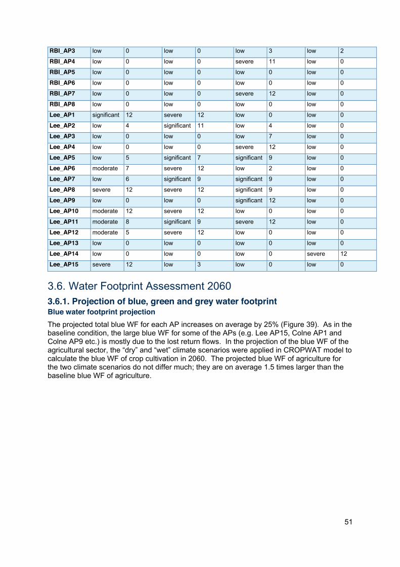
51

RBI_AP3 low 0 low 0 low 3 low 2

RBI_AP4 low 0 low 0 severe 11 low 0

RBI_AP5 low 0 low 0 low 0 low 0

RBI_AP6 low 0 low 0 low 0 low 0

RBI_AP7 low 0 low 0 severe 12 low 0

RBI_AP8 low 0 low 0 low 0 low 0

Lee_AP1 significant 12 severe 12 low 0 low 0

Lee_AP2 low 4 significant 11 low 4 low 0

Lee_AP3 low 0 low 0 low 7 low 0

Lee_AP4 low 0 low 0 severe 12 low 0

Lee_AP5 low 5 significant 7 significant 9 low 0

Lee_AP6 moderate 7 severe 12 low 2 low 0

Lee_AP7 low 6 significant 9 significant 9 low 0

Lee_AP8 severe 12 severe 12 significant 9 low 0

Lee_AP9 low 0 low 0 significant 12 low 0

Lee_AP10 moderate 12 severe 12 low 0 low 0

Lee_AP11 moderate 8 significant 9 severe 12 low 0

Lee_AP12 moderate 5 severe 12 low 0 low 0

Lee_AP13 low 0 low 0 low 0 low 0

Lee_AP14 low 0 low 0 low 0 severe 12

Lee_AP15 severe 12 low 3 low 0 low 0

3.6. Water Footprint Assessment 2060 3.6.1. Projection of blue, green and grey water footprint Blue water footprint projection The projected total blue WF for each AP increases on average by 25% (Figure 39). As in the baseline condition, the large blue WF for some of the APs (e.g. Lee AP15, Colne AP1 and Colne AP9 etc.) is mostly due to the lost return flows. In the projection of the blue WF of the agricultural  sector,  the  “dry”  and  “wet”  climate  scenarios  were  applied  in  CROPWAT  model  to  calculate the blue WF of crop cultivation in 2060. The projected blue WF of agriculture for the two climate scenarios do not differ much; they are on average 1.5 times larger than the baseline blue WF of agriculture.

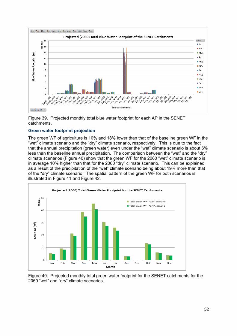
52

Figure 39. Projected monthly total blue water footprint for each AP in the SENET catchments.

Green water footprint projection The green WF of agriculture is 10% and 18% lower than that of the baseline green WF in the “wet”  climate scenario  and  the  “dry”  climate scenario, respectively. This is due to the fact that  the  annual  precipitation  (green  water)  even  under  the  “wet”  climate scenario is about 6% less  than  the  baseline  annual  precipitation.    The  comparison  between  the  “wet”  and  the  “dry”  climate scenarios (Figure 40)  show  that  the  green  WF  for  the  2060  “wet”  climate  scenario  is  in  average  10%  higher  than  that  for  the  2060  “dry”  climate  scenario.    This  can be explained as  a  result  of  the  precipitation  of  the  “wet”  climate  scenario  being  about  19%  more  than  that  of  the  “dry”  climate  scenario.    The  spatial  pattern  of  the  green  WF  for  both  scenarios  is  illustrated in Figure 41 and Figure 42.

Figure 40. Projected monthly total green water footprint for the SENET catchments for the 2060  “wet”  and  “dry”  climate  scenarios.

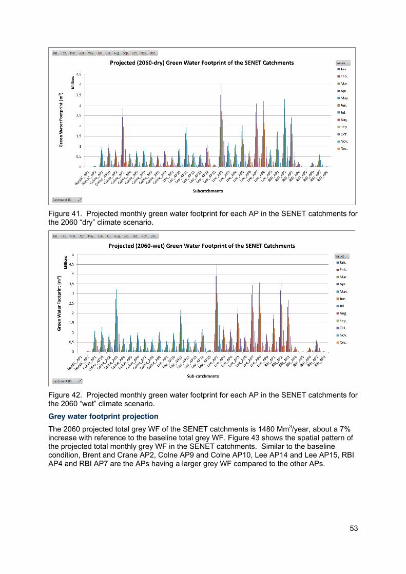
53

Figure 41. Projected monthly green water footprint for each AP in the SENET catchments for the  2060  “dry”  climate  scenario.

Figure 42. Projected monthly green water footprint for each AP in the SENET catchments for the  2060  “wet”  climate  scenario.

Grey water footprint projection The 2060 projected total grey WF of the SENET catchments is 1480 Mm3/year, about a 7% increase with reference to the baseline total grey WF. Figure 43 shows the spatial pattern of the projected total monthly grey WF in the SENET catchments. Similar to the baseline condition, Brent and Crane AP2, Colne AP9 and Colne AP10, Lee AP14 and Lee AP15, RBI AP4 and RBI AP7 are the APs having a larger grey WF compared to the other APs.

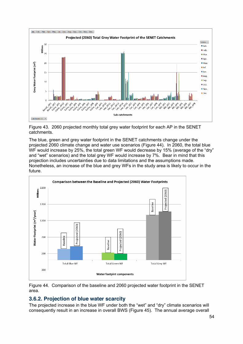
54

Figure 43. 2060 projected monthly total grey water footprint for each AP in the SENET catchments.

The blue, green and grey water footprint in the SENET catchments change under the projected 2060 climate change and water use scenarios (Figure 44). In 2060, the total blue WF  would  increase  by  25%,  the  total  green  WF  would  decrease  by  15%  (average  of  the  “dry”  and  “wet”  scenarios)  and  the  total  grey  WF  would  increase by 7%. Bear in mind that this projection includes uncertainties due to data limitations and the assumptions made. Nonetheless, an increase of the blue and grey WFs in the study area is likely to occur in the future.

Figure 44. Comparison of the baseline and 2060 projected water footprint in the SENET area.

3.6.2. Projection of blue water scarcity The  projected  increase  in  the  blue  WF  under  both  the  “wet”  and  “dry”  climate  scenarios  will  consequently result in an increase in overall BWS (Figure 45). The annual average overall

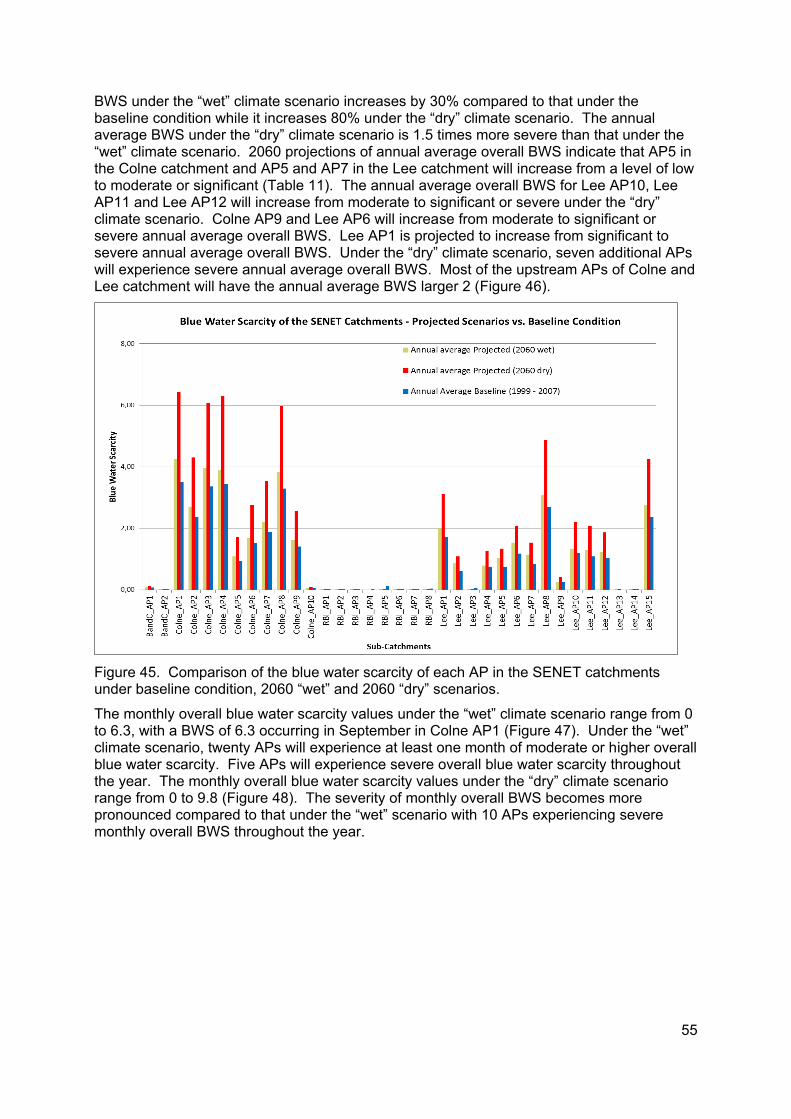
55

BWS  under  the  “wet”  climate  scenario  increases  by  30%  compared  to  that  under  the  baseline condition while  it  increases  80%  under  the  “dry”  climate  scenario.    The  annual  average  BWS  under  the  “dry”  climate  scenario  is  1.5  times  more  severe  than  that  under  the  “wet”  climate  scenario.    2060  projections  of  annual  average  overall  BWS  indicate  that  AP5  in  the Colne catchment and AP5 and AP7 in the Lee catchment will increase from a level of low to moderate or significant (Table 11). The annual average overall BWS for Lee AP10, Lee AP11  and  Lee  AP12  will  increase  from  moderate  to  significant  or  severe  under  the  “dry”  climate scenario. Colne AP9 and Lee AP6 will increase from moderate to significant or severe annual average overall BWS. Lee AP1 is projected to increase from significant to severe  annual  average  overall  BWS.    Under  the  “dry”  climate  scenario,  seven  additional  APs  will experience severe annual average overall BWS. Most of the upstream APs of Colne and Lee catchment will have the annual average BWS larger 2 (Figure 46).

Figure 45. Comparison of the blue water scarcity of each AP in the SENET catchments under  baseline  condition,  2060  “wet”  and  2060  “dry”  scenarios.

The monthly overall blue water scarcity values under  the  “wet”  climate scenario range from 0 to 6.3, with a BWS of 6.3 occurring in September in Colne AP1 (Figure 47). Under  the  “wet”  climate scenario, twenty APs will experience at least one month of moderate or higher overall blue water scarcity. Five APs will experience severe overall blue water scarcity throughout the year. The monthly overall blue water scarcity values under the  “dry”  climate scenario range from 0 to 9.8 (Figure 48). The severity of monthly overall BWS becomes more pronounced compared to that under the  “wet”  scenario with 10 APs experiencing severe monthly overall BWS throughout the year.

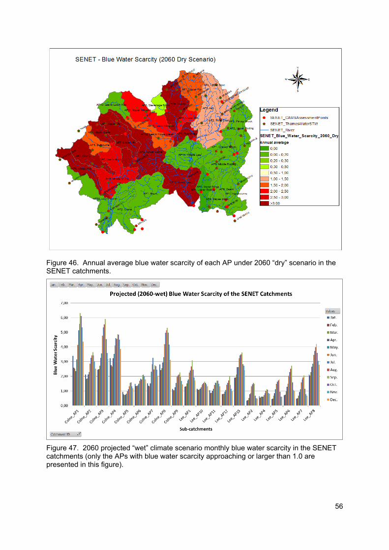
56

Figure 46. Annual average blue water scarcity of each AP under  2060  “dry”  scenario  in  the  SENET catchments.

Figure 47. 2060  projected  “wet”  climate  scenario  monthly  blue  water  scarcity  in  the  SENET  catchments (only the APs with blue water scarcity approaching or larger than 1.0 are presented in this figure).

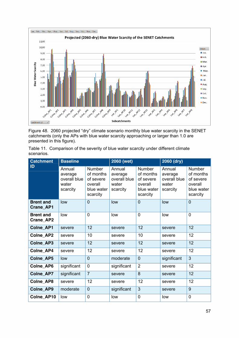
57

Figure 48.    2060  projected  “dry”  climate scenario monthly blue water scarcity in the SENET catchments (only the APs with blue water scarcity approaching or larger than 1.0 are presented in this figure).

Table 11. Comparison of the severity of blue water scarcity under different climate scenarios.

Catchment ID

Baseline 2060 (wet) 2060 (dry) Annual average overall blue water scarcity

Number of months of severe overall blue water scarcity

Annual average overall blue water scarcity

Number of months of severe overall blue water scarcity

Annual average overall blue water scarcity

Number of months of severe overall blue water scarcity

Brent and Crane_AP1

low 0 low 0 low 0

Brent and Crane_AP2

low 0 low 0 low 0

Colne_AP1 severe 12 severe 12 severe 12

Colne_AP2 severe 10 severe 10 severe 12

Colne_AP3 severe 12 severe 12 severe 12

Colne_AP4 severe 12 severe 12 severe 12

Colne_AP5 low 0 moderate 0 significant 3

Colne_AP6 significant 0 significant 2 severe 12

Colne_AP7 significant 7 severe 8 severe 12

Colne_AP8 severe 12 severe 12 severe 12

Colne_AP9 moderate 0 significant 3 severe 9

Colne_AP10 low 0 low 0 low 0

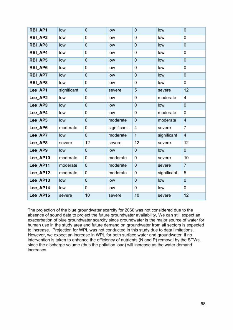
58

RBI_AP1 low 0 low 0 low 0

RBI_AP2 low 0 low 0 low 0

RBI_AP3 low 0 low 0 low 0

RBI_AP4 low 0 low 0 low 0

RBI_AP5 low 0 low 0 low 0

RBI_AP6 low 0 low 0 low 0

RBI_AP7 low 0 low 0 low 0

RBI_AP8 low 0 low 0 low 0

Lee_AP1 significant 0 severe 5 severe 12

Lee_AP2 low 0 low 0 moderate 4

Lee_AP3 low 0 low 0 low 0

Lee_AP4 low 0 low 0 moderate 0

Lee_AP5 low 0 moderate 0 moderate 4

Lee_AP6 moderate 0 significant 4 severe 7

Lee_AP7 low 0 moderate 1 significant 4

Lee_AP8 severe 12 severe 12 severe 12

Lee_AP9 low 0 low 0 low 0

Lee_AP10 moderate 0 moderate 0 severe 10

Lee_AP11 moderate 0 moderate 0 severe 7

Lee_AP12 moderate 0 moderate 0 significant 5

Lee_AP13 low 0 low 0 low 0

Lee_AP14 low 0 low 0 low 0

Lee_AP15 severe 10 severe 10 severe 12

The projection of the blue groundwater scarcity for 2060 was not considered due to the absence of sound data to project the future groundwater availability, We can still expect an exacerbation of blue groundwater scarcity since groundwater is the major source of water for human use in the study area and future demand on groundwater from all sectors is expected to increase. Projection for WPL was not conducted in this study due to data limitations. However, we expect an increase in WPL for both surface water and groundwater, if no intervention is taken to enhance the efficiency of nutrients (N and P) removal by the STWs, since the discharge volume (thus the pollution load) will increase as the water demand increases.

59

4. Recommendations on water footprint response strategies The aim of WFA is to understand where a WF is located, how large that WF is and whether the WF is sustainable or not. Results should feed into formulating response strategies. WFA can be used to identify priority places to work and provides insight into strategic actions to be taken to reduce the WF and to make it sustainable. Using the WF accounting and sustainability assessment presented in sections 3.1, 3.2, 3.3 and 3.5 APs in need of WF reduction strategies have been determined (Table 12). Response strategies can be formulated to address the key sustainability issues for each AP, for example, surface and/or groundwater scarcity and surface and/or groundwater pollution levels. This comprehensive analysis of multiple criteria also illuminates the possible interrelationships between blue water scarcity and water pollution levels. These linkages can be addressed in response formulation resulting in the optimal outcome from the actions taken.

Water footprint response strategies should be developed for each specific case to provide the most benefit¸ however, a general approach to response formulation is:

• Industrial water users: implement better or best technologies which reduce evaporation loss (blue WF) in the production processes and minimise the pollution load (grey WF);

• Agricultural water users: implement better irrigation methods and precision irrigation scheduling to reduce unproductive evaporation (blue WF); add soil treatments to more effectively use rainwater (green WF); and apply integrated crop nutrient management practices to reduce non-point source pollution (grey WF);

• Domestic water users: use low flow devices in the home, plant native plants in landscaping (blue WF) and reduce the use of chemicals in the household and in lawn and garden care (grey WF); and

• Water utilities: re-evaluate the current drinking water distribution networks and sewage treatment works and study the feasibility of re-planning both systems to avoid or reduce water transfer (return flows) therefore blue water footprint as a result of transporting water outside the sub-catchments where water is abstracted.

Regulatory agencies: aim for demand management within the constraints required to meet sustainability criteria such as blue water scarcity and water pollution levels, recognising the relationships between them. Combined together these response strategies can lead to an overall improvement in the sustainability of water use in catchments.

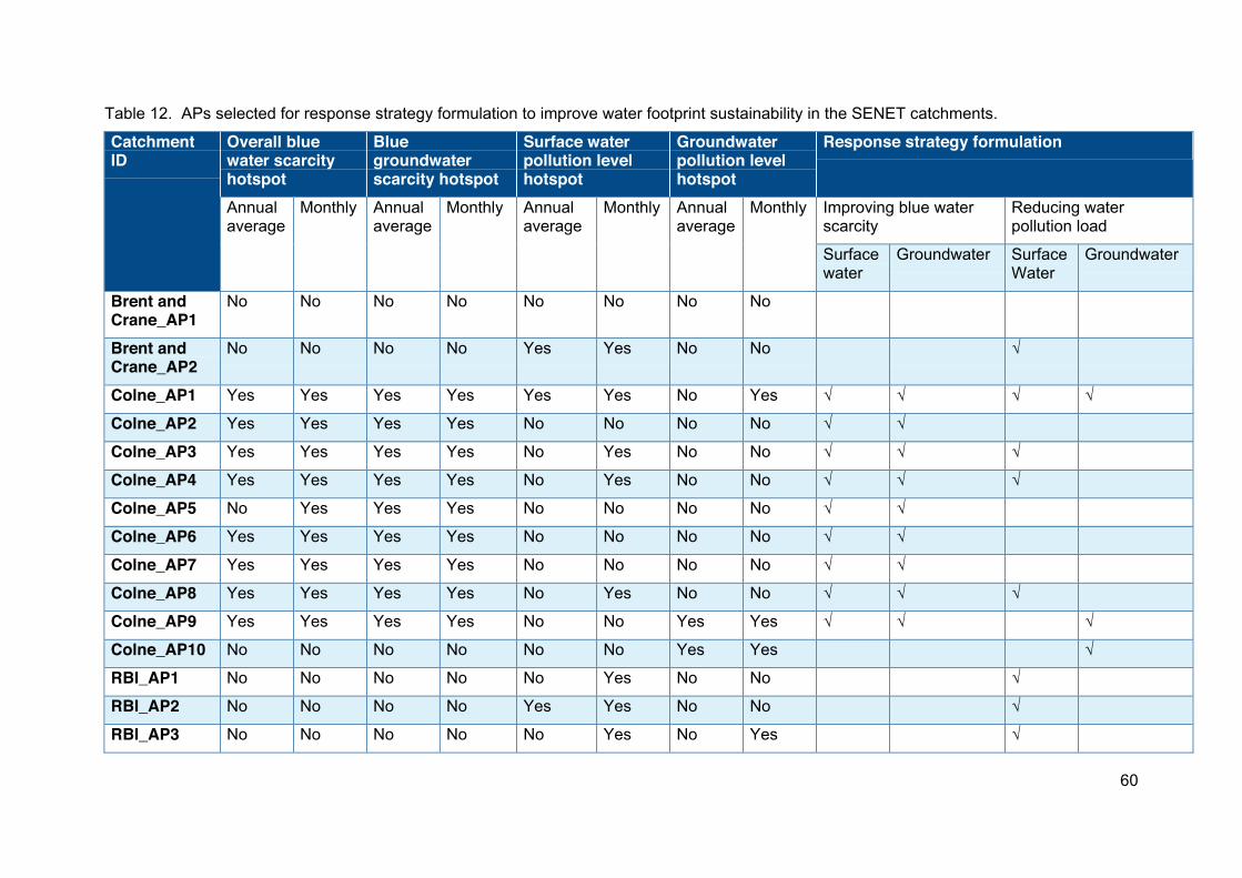
60

Table 12. APs selected for response strategy formulation to improve water footprint sustainability in the SENET catchments.

Catchment ID

Overall blue water scarcity hotspot

Blue groundwater scarcity hotspot

Surface water pollution level hotspot

Groundwater pollution level hotspot

Response strategy formulation

Annual average

Monthly Annual average

Monthly Annual average

Monthly Annual average

Monthly Improving blue water scarcity

Reducing water pollution load

Surface water

Groundwater Surface Water

Groundwater

Brent and Crane_AP1

No No No No No No No No

Brent and Crane_AP2

No No No No Yes Yes No No √

Colne_AP1 Yes Yes Yes Yes Yes Yes No Yes √ √ √ √

Colne_AP2 Yes Yes Yes Yes No No No No √ √

Colne_AP3 Yes Yes Yes Yes No Yes No No √ √ √

Colne_AP4 Yes Yes Yes Yes No Yes No No √ √ √

Colne_AP5 No Yes Yes Yes No No No No √ √

Colne_AP6 Yes Yes Yes Yes No No No No √ √

Colne_AP7 Yes Yes Yes Yes No No No No √ √

Colne_AP8 Yes Yes Yes Yes No Yes No No √ √ √

Colne_AP9 Yes Yes Yes Yes No No Yes Yes √ √ √

Colne_AP10 No No No No No No Yes Yes √

RBI_AP1 No No No No No Yes No No √

RBI_AP2 No No No No Yes Yes No No √

RBI_AP3 No No No No No Yes No Yes √

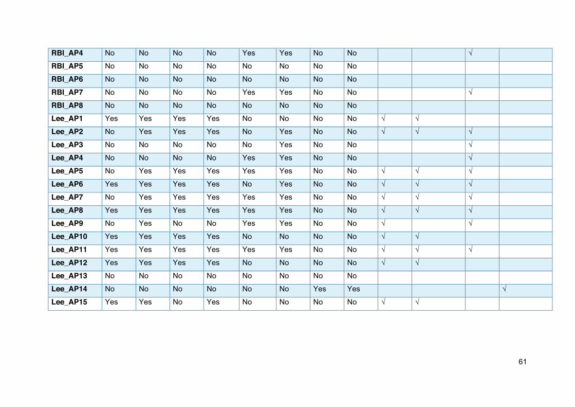
61

RBI_AP4 No No No No Yes Yes No No √

RBI_AP5 No No No No No No No No

RBI_AP6 No No No No No No No No

RBI_AP7 No No No No Yes Yes No No √

RBI_AP8 No No No No No No No No

Lee_AP1 Yes Yes Yes Yes No No No No √ √

Lee_AP2 No Yes Yes Yes No Yes No No √ √ √

Lee_AP3 No No No No No Yes No No √

Lee_AP4 No No No No Yes Yes No No √

Lee_AP5 No Yes Yes Yes Yes Yes No No √ √ √

Lee_AP6 Yes Yes Yes Yes No Yes No No √ √ √

Lee_AP7 No Yes Yes Yes Yes Yes No No √ √ √

Lee_AP8 Yes Yes Yes Yes Yes Yes No No √ √ √

Lee_AP9 No Yes No No Yes Yes No No √ √

Lee_AP10 Yes Yes Yes Yes No No No No √ √

Lee_AP11 Yes Yes Yes Yes Yes Yes No No √ √ √

Lee_AP12 Yes Yes Yes Yes No No No No √ √

Lee_AP13 No No No No No No No No

Lee_AP14 No No No No No No Yes Yes √

Lee_AP15 Yes Yes No Yes No No No No √ √

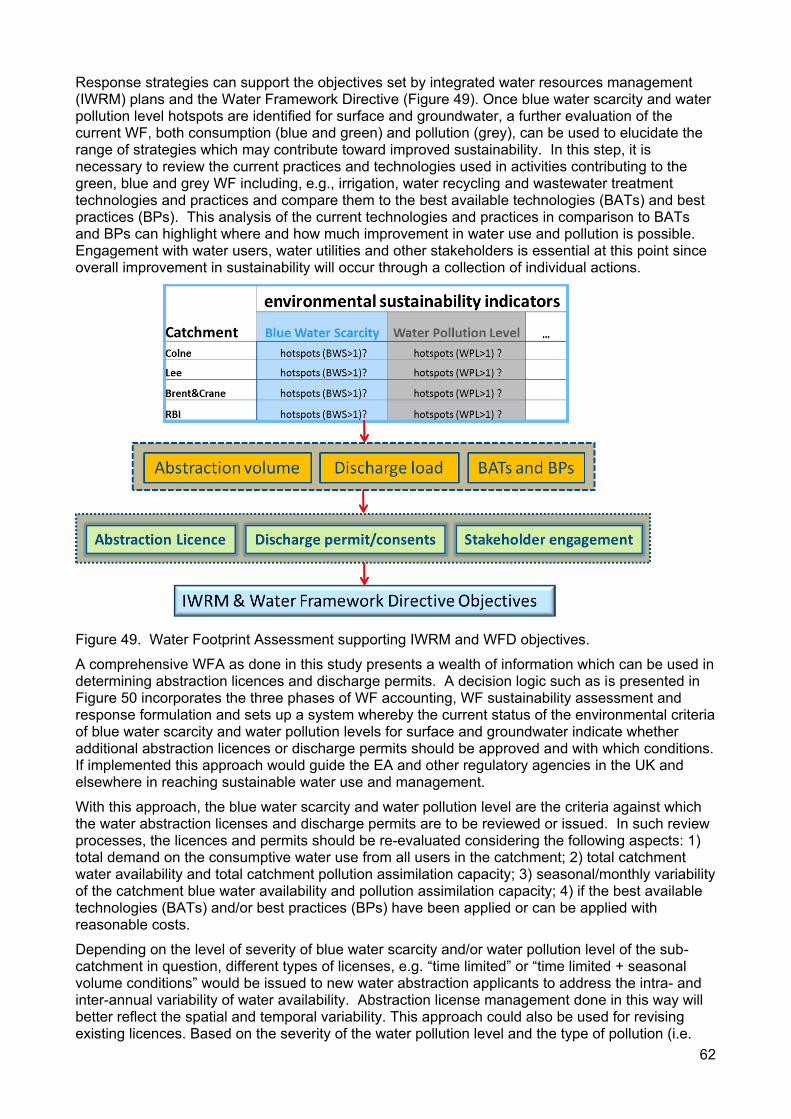
62

Response strategies can support the objectives set by integrated water resources management (IWRM) plans and the Water Framework Directive (Figure 49). Once blue water scarcity and water pollution level hotspots are identified for surface and groundwater, a further evaluation of the current WF, both consumption (blue and green) and pollution (grey), can be used to elucidate the range of strategies which may contribute toward improved sustainability. In this step, it is necessary to review the current practices and technologies used in activities contributing to the green, blue and grey WF including, e.g., irrigation, water recycling and wastewater treatment technologies and practices and compare them to the best available technologies (BATs) and best practices (BPs). This analysis of the current technologies and practices in comparison to BATs and BPs can highlight where and how much improvement in water use and pollution is possible. Engagement with water users, water utilities and other stakeholders is essential at this point since overall improvement in sustainability will occur through a collection of individual actions.

Figure 49. Water Footprint Assessment supporting IWRM and WFD objectives.

A comprehensive WFA as done in this study presents a wealth of information which can be used in determining abstraction licences and discharge permits. A decision logic such as is presented in Figure 50 incorporates the three phases of WF accounting, WF sustainability assessment and response formulation and sets up a system whereby the current status of the environmental criteria of blue water scarcity and water pollution levels for surface and groundwater indicate whether additional abstraction licences or discharge permits should be approved and with which conditions. If implemented this approach would guide the EA and other regulatory agencies in the UK and elsewhere in reaching sustainable water use and management.

With this approach, the blue water scarcity and water pollution level are the criteria against which the water abstraction licenses and discharge permits are to be reviewed or issued. In such review processes, the licences and permits should be re-evaluated considering the following aspects: 1) total demand on the consumptive water use from all users in the catchment; 2) total catchment water availability and total catchment pollution assimilation capacity; 3) seasonal/monthly variability of the catchment blue water availability and pollution assimilation capacity; 4) if the best available technologies (BATs) and/or best practices (BPs) have been applied or can be applied with reasonable costs.

Depending on the level of severity of blue water scarcity and/or water pollution level of the sub-catchment in question, different types of licenses, e.g. “time  limited”  or  “time  limited  + seasonal volume  conditions” would be issued to new water abstraction applicants to address the intra- and inter-annual variability of water availability. Abstraction license management done in this way will better reflect the spatial and temporal variability. This approach could also be used for revising existing licences. Based on the severity of the water pollution level and the type of pollution (i.e.

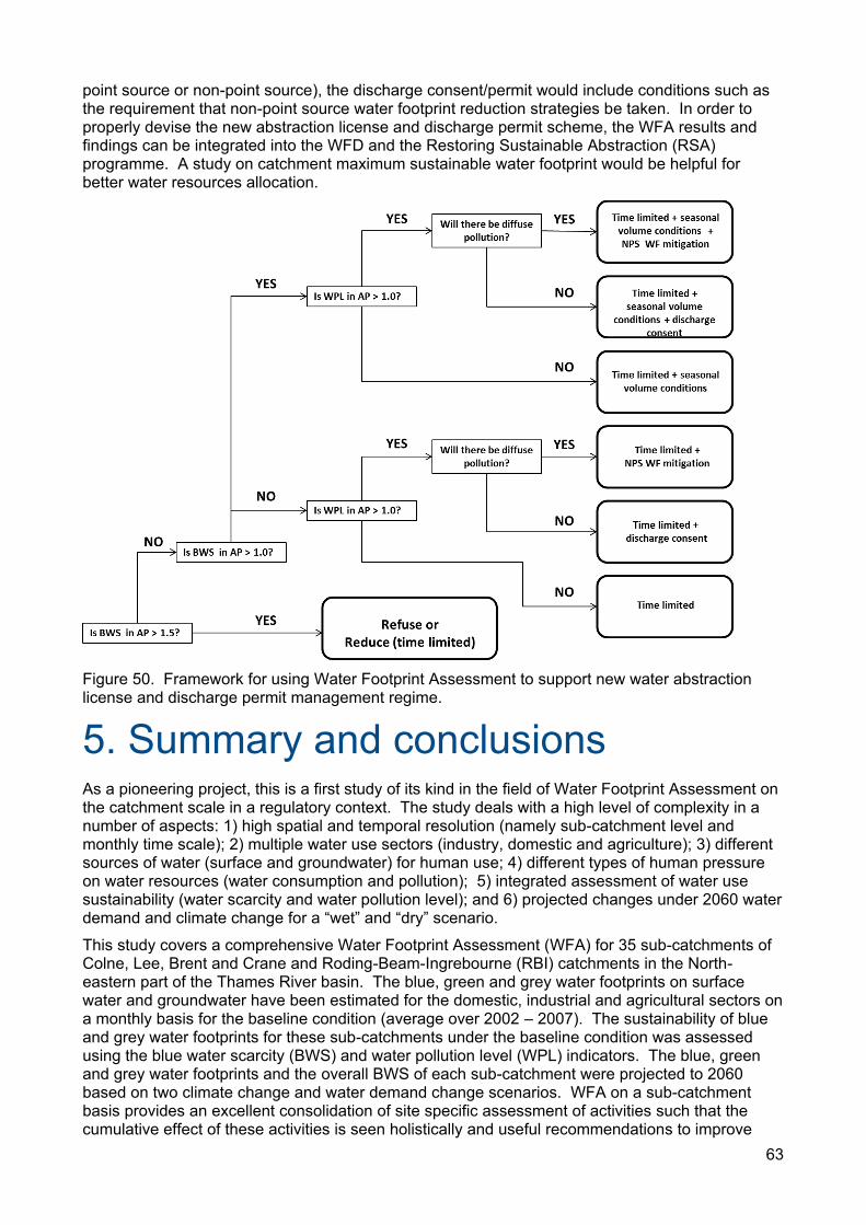
63

point source or non-point source), the discharge consent/permit would include conditions such as the requirement that non-point source water footprint reduction strategies be taken. In order to properly devise the new abstraction license and discharge permit scheme, the WFA results and findings can be integrated into the WFD and the Restoring Sustainable Abstraction (RSA) programme. A study on catchment maximum sustainable water footprint would be helpful for better water resources allocation.

Figure 50. Framework for using Water Footprint Assessment to support new water abstraction license and discharge permit management regime.

5. Summary and conclusions As a pioneering project, this is a first study of its kind in the field of Water Footprint Assessment on the catchment scale in a regulatory context. The study deals with a high level of complexity in a number of aspects: 1) high spatial and temporal resolution (namely sub-catchment level and monthly time scale); 2) multiple water use sectors (industry, domestic and agriculture); 3) different sources of water (surface and groundwater) for human use; 4) different types of human pressure on water resources (water consumption and pollution); 5) integrated assessment of water use sustainability (water scarcity and water pollution level); and 6) projected changes under 2060 water demand  and  climate  change  for  a  “wet”  and  “dry”  scenario.

This study covers a comprehensive Water Footprint Assessment (WFA) for 35 sub-catchments of Colne, Lee, Brent and Crane and Roding-Beam-Ingrebourne (RBI) catchments in the North-eastern part of the Thames River basin. The blue, green and grey water footprints on surface water and groundwater have been estimated for the domestic, industrial and agricultural sectors on a monthly basis for the baseline condition (average over 2002 – 2007). The sustainability of blue and grey water footprints for these sub-catchments under the baseline condition was assessed using the blue water scarcity (BWS) and water pollution level (WPL) indicators. The blue, green and grey water footprints and the overall BWS of each sub-catchment were projected to 2060 based on two climate change and water demand change scenarios. WFA on a sub-catchment basis provides an excellent consolidation of site specific assessment of activities such that the cumulative effect of these activities is seen holistically and useful recommendations to improve

64

water management can be derived. From the baseline and projected WFA results, recommendations for water footprint response strategies were put forward.

5.1. Summary of the current WFA study 5.1.1. Baseline blue water footprint Under the baseline condition, the blue WF of all sub-catchments in the study area sums up to 338 Mm3/year (or 105 mm/year), of which 1.43 Mm3/year (0.4 mm/year) is for the industrial sector, 334 Mm3/year (104 mm/year) for domestic sector and 2.75 Mm3/year (0.9 mm/year) for the agricultural sector, respectively. The domestic sector is by far the largest water consuming sector. The blue WF of all sub-catchments resulting from groundwater use is approximately 55% of the total blue WF. Ninety five percent this total blue WF is due to the lost return flows (non-evaporative losses) within and beyond the study area. The actual total blue WF of the study area, namely the total evaporative blue WF plus the return flows lost to outside the study area as a whole, is 62 Mm3/year (19.4 mm/year), while the evaporative blue WF is only 16.5 Mm3/year (5.1 mm/year). Around 80% of the total return flows remain within the study area and these return flows are transferred from one sub-catchment to (an) other sub-catchment(s) via pipelines of the sewage treatment works.

5.1.2. Implications of transporting the return flows through sewage treatment works to other sub-catchments The return flows, collected and transported to the sewage treatment works that are not situated in the sub-catchment of water abstraction, have strong implications for both water-losing and water-receiving sub-catchments in terms of the blue water availability and water pollution. In the sub-catchments losing return flows, environmental flows are violated and less water is available to assimilate waste although the pollution load is reduced. On the other hand, the sub-catchments receiving the lost return flows have more blue water available, but the pollution load is increased. Twenty sub-catchments (nine from Colne catchment and ten from Lee catchment and one from Brent and Crane catchment) are net water losing sub-catchments while six sub-catchments (four from Lee catchment, one from RBI catchment and one from Colne catchment) are net water receiving sub-catchments. Most of the net water losing sub-catchments generally have high blue water scarcity while those that are net water receiving sub-catchments generally have a high water pollution level.

5.1.3. Baseline green water footprint In the estimation of crop water consumption, five major crops cultivated in the study area were taken into account. The baseline green WF in the study area totals 225 Mm3/year (70 mm/year). The green WF is 99% of the total crop water consumption. The upstream sub-catchments of the study area, with more extensive agricultural lands, have a larger green WF than the more urbanised downstream sub-catchments.

5.1.4. Baseline grey water footprint The total baseline grey WF amounts to 1380 Mm3/year, equivalent to 428 mm/year. The total grey WF of point-source pollution on surface water is 408 Mm3/year (127 mm/year); the total grey WF of the point-source pollution on groundwater is 664 Mm3/year (207 mm/year); and the total grey WF of the non-point source pollution due to fertiliser leaching is 304 Mm3/year (95 mm/year). The grey WF of the point-source pollution on groundwater, almost 50% of the total grey WF of the study area, is 1.6 times larger than that of the point-source pollution on surface water.

The grey WF is mostly due to the pollution of nutrients (phosphorous and nitrogen). High grey WF occurs in the sub-catchments where large scale and/or a higher number of sewage treatment works are located, and when large amounts of effluent are used for recharge to groundwater, resulting in high pollution loads. These sub-catchments are Brent and Crane AP2, Colne AP3, Colne AP9, Colne AP10, Lee AP2, Lee AP14, Lee AP15, RBI AP4 and RBI AP7. Large grey WFs resulting from non-point source pollution generally occur from the farm lands in the upstream sub-catchments.

65

5.1.5. Baseline blue water scarcity Under the baseline condition, eight Colne sub-catchments and seven Lee sub-catchments are experiencing a moderate or higher level of overall blue water scarcity. Amongst these, the upstream sub-catchments are experiencing severe overall blue water scarcity. The blue groundwater scarcity in the sub-catchments under study is more severe than the overall blue water scarcity. Nine Colne sub-catchments and nine Lee sub-catchments have annual average blue groundwater scarcity at the significant or severe level. The blue groundwater scarcity values of many upstream sub-catchments are even larger than 5 indicating that abstraction is far exceeding renewable groundwater supplies. The majority of the sub-catchments with overall blue water scarcity or blue groundwater scarcity at the moderate or higher level are those having lost return flows. Sub-catchments in RBI experience low blue water scarcity for both surface and ground water.

5.1.6. Baseline water pollution level Under the baseline condition, 12 sub-catchments in the study area have the annual average surface water pollution level at the significant or severe level (WPL>1). Sewage treatment works in these sub-catchments collect more wastewater than the other sub-catchments. These sewage works treat the wastewater and then discharge the effluents into streams, generating high WPL for surface water. Three sub-catchments (two in Colne catchment and one in Lee catchment) have annual average groundwater WPL at the significant or severe level. The groundwater assimilation capacity in these sub-catchments is under high pressure due to the recharge or infiltration of treated effluent with high loads of ammonia-nitrogen.

5.1.7. Water footprint projection The blue, green and grey WF and blue water scarcity were projected to 2060 based on two climate change and water demand change scenarios. The blue WF projected for all 35 sub-catchments is 424 Mm3/year (132 mm/year), which is a 25% increase compared to the baseline blue WF. The projected total green WF is 205 Mm3/year  (64  mm/year)  for  the  “wet”  climate scenario and 184 Mm3/year  (57  mm/year)  for  the  “dry”  climate scenario. The projected green WF is 14% lower than the baseline green WF. The projected total grey WF is 1480 Mm3/year (460 mm/year), about 7% higher than the baseline total grey WF.

With  the  “dry”  scenario,  the  projected  overall  blue  water  scarcity  becomes  more  severe  across  the  SENET Area. Under this condition, there are five more sub-catchments, four in the upstream of the Lee catchment and one in the upstream Colne catchment, having the blue water scarcity exceeding the moderate level, when compared to the baseline blue water scarcity situation. Even with  the  “wet”  scenario,  the  blue  water  scarcity  becomes  worse  when  compared  with  the  baseline  condition.

5.1.8. Recommendation for response strategies A step-wise approach using multiple environmental sustainability indicators (i.e. blue water scarcity and water pollution level) was used to identify the APs in need of WF reduction strategies to address surface and/or groundwater scarcity and surface and/or groundwater pollution levels. A new water abstraction license and discharge permit management system based on the results of this WFA was proposed as a way to meet sustainable water use and management goals as set out in the WFD and IWRM plans. A new abstraction license and discharge permit system such as this will enable a dynamic linkage to the spatial and temporal variability of blue water availability and the assimilation capacity for pollution loads.

5.2. Conclusions and recommended future work Over-withdrawal and pollution have led to inadequate functioning of three-fourths of the rivers and lakes in England and Wales (Defra, 2011). The combined effects of climate change and growing demand on water will put more pressure on the existing water resources. The interactions between human usage, management of water and the response of nature to such human activities are complex. Therefore, we need various tools to assist us in coping with the challenges in managing these precious water resources. WFA is such a tool and is useful in helping us better understand what and where the pressures on freshwater resources are and what changes are

66

necessary to improve the sustainability, efficiency and equitability of water use. From this WFA study, we have obtained a clear picture depicting how the surface water and groundwater are consumed by the industrial, domestic and agricultural sectors. This WFA also clearly illustrates where and when such water use creates problems: decrease of water availability (blue water scarcity) and diminishing of waste assimilation capacity (water pollution level).

On the basis of the findings of this WFA study, we can conclude the following:

• WFA is a holistic tool unifying both quantity and quality aspects in water resources assessment, planning and management.

• The choice of using the Assessment Point (AP), i.e. sub-catchment scale, provided added value by consolidating individual activities such that the aggregated or cumulative effect could be seen and the cause-effect relationships could be identified.

• WFA looks at the water quality issue from the pollution load rather than only the pollutant concentration in the effluents using the waste assimilation approach. This highlights where the assimilation capacity has been exceeded even when the pollutant concentrations meet quality standards.

• WFA uses environmental flow requirements (EFR) to evaluate how water consumption leads to freshwater (blue water) scarcity. The EFR concept agrees well with the environmental flow indicator (EFI) widely applied in the WFD of England and Wales.

• This WFA study explored the effect of return flows through sewage treatment works on both blue water scarcity and water pollution levels at the sub-catchment level. This exploration may suggest a possible strategy to cope with climate change and future water demand increases.

• The WFA results make the spatial and temporal nature of water consumption and pollution explicit. This can form a sound factual basis for reforming abstraction licences and discharge permits. The information developed in this study can also function as a platform or as an instrument for discussion and dialogue between regulators, water utilities and water users.

• The WFA study results can be the foundation for a unified water footprint database that is complementary to the existing water resources statistics and management system. A catchment-scale water footprint database can be an integrated element in the future update of the Catchment Abstraction Management Strategies (CAMS).

• The WFA concept brought together the data from multiple data sources directly available within the EA and demonstrated the added value of using combined data to understand the water resource situation in SENET.

• High overall blue water scarcity hotspots mostly lie in the upstream Colne and Lee catchments. Blue groundwater scarcity is more pronounced than the overall blue water scarcity because of the higher dependency of the water use on groundwater resources.

• Water pollution level hotspots are mostly those sub-catchments where large-scale and/or a higher number of sewage treatment works are located. The current study indicates that the nutrient (nitrogen and phosphorous) load is the major pressure on the water system from the quality perspective.

• The  overall  blue  water  scarcity  under  both  the  “wet”  and  “dry”  climate  scenarios  will  increase  compared to that under baseline condition.

• Water footprint sustainability based demand management is an innovative approach to reforming the current water abstraction license and discharge permit scheme and can be an effective response strategy to mitigate blue water scarcity and water pollution levels.

To further improve water resources and abstraction management, a list of possible further work is recommended as follows.

• Integrate WFA into the implementation of the Water Framework Directive (WFD). • Apply WFA to support the Restoring Sustainable Abstraction (RSA) programme and in the

abstraction licence reform carried out by the Environment Agency. • Roll out WFA studies to all management regions of the Environment Agency. • Enhance the wastewater treatment technologies to increase nutrient removal efficiency.

67

• Study the feasibility of planning sewage treatment works in those sub-catchments which currently have to transport their wastewater and sewage to the treatment works located in other sub-catchments or of effluent discharges returning to the originating sub-catchment.

• Understand how drinking water distribution networks, operated by drinking water companies, can help minimise lost return flow and therefore blue water footprint.

• Improve data collection and data storage systems to facilitate data processing for easy and efficient Water Footprint Assessment and for other water resources assessment studies.

• Improve the blue water scarcity assessment by using monthly variable EFIs which take into account more detailed river flow regime variability better reflecting the relationship between flow dynamics and the ecosystem health of the water bodies. This also can be helpful for design and implementation of an abstraction incentive mechanism (e.g. Fenn, 2012).

• Establish water consumption and pollution benchmarks per sector and water footprint caps per catchment to drive water use efficiency, wastewater treatment enhancement, and better water allocation to ensure that water consumption and pollution remain below the maximum sustainable level.

• Update the current water availability and water scarcity maps using the WFA approach, i.e. applying the spatially and temporally varying EFRs (or EFIs). This can better support future water abstraction demand management and restrict unessential abstraction especially during the low flows and drought spells.

• Improve the groundwater scarcity and pollution level analysis through further research on groundwater sustainable yield, groundwater flows and aquifer properties in the study area.

• Improve grey water footprint assessment by taking into account the non-point source pollution from urban areas, roads and other built areas.

• Conduct further study on a new abstraction licencing and discharge permitting system based on the initial recommendation made in this study and how these changes would ensure the sustainable use and management of water resources.

68

References Acreman, M. C. and Dunbar, M. J., 2004. Defining environmental river flow requirements - a review. Hydrol. Earth Syst. Sci., 8, 861-876, doi:10.5194/hess-8-861-2004.

Alley, W.M. and Leake, S.A., 2004. The Journey from Safe Yield to Sustainability. Ground Water, 42(1), 12-16.

Alley, W.M., Reilly, T.E. and Franke, O.L., 1999. Sustainability of ground-water resources. U.S. Geological Survey Circular 1186.

Bloomfield, J.P., Bricker, S.H. and Newell, A.J., 2011. Some relationships between lithology, basin form and hydrology: a case study from the Thames basin. UK, Hydrol. Process, 25, 2518–2530, doi: 10.1002/hyp.8024.

British Geological Survey, Groundwater resources, UK Groundwater Forum [online]. Available from: http://www.groundwateruk.org/Groundwater-in-depth.aspx, [Accessed 26 March 2012].

Davison, P.S., Withers, P.J.A., Lord, E.I., Betson, M.J. and Strömqvist, J., 2008. PSYCHIC- A process-based model of phosphorus and sediment mobilisation and delivery within agricultural catchments. Part 1: Model description and parameterisation. Journal of Hydrology, 350, 290 -302.

Defra,  2011,  Water  for  Life,  Her  Majesty’s  Stationery  Office,  ISBN:  9780101823029.

De Vos, W. and Tarvainen, T. (Chief-editors), 2006. Geochemical Atlas of Europe, Part 2: Interpretation of geochemical maps, additional tables, figures, maps, and related publications [online]. Available from: http://weppi.gtk.fi/publ/foregsatlas/part2.php ISBN: 951-690-956-6 [Accessed 22 July 2014].

Dunbar, M.J., Acreman, M. and Kirk, S., 2004. Environmental flow setting in England and Wales: strategies for managing abstraction in catchments. Water & Environ. J., 18 (1), 5-10.

Environment Agency, 2009. Conceptualisation report for the RBI CAMS.

Environment Agency, 2010a. Conceptualisation report for the Colne CAMS (Version number: 1.0).

Environment Agency, 2010b. Conceptualisation report for the Lee CAMS (Version number: 1.3).

Environment Agency, 2011. Conceptualisation report for North London CAMS.

Environment Agency, 2013a. Environmental Flow Indicator (unclassified document).

Environment Agency, 2013b. Review of Good Practice Guidelines for run-of-river hydropower schemes - Supplementary consultation on river flow and water abstraction standards.

Environmental Agency and Ofwat, 2011. The case for change – reforming water abstraction management in England. Report GEHO1111BVEQ-E-E.

Fenn C., 2012. Report to Ofwat on application testing of a prototype design of the abstraction incentive mechanism (AIM). CFonstream, UK.

Hoekstra, A.Y., Chapagain, A.K., Aldaya, M.M. and Mekonnen, M.M., 2011. The water footprint assessment manual: Setting the global standard. Earthscan, London, UK, ISBN: 978-1-84971-279-8.

Hoekstra, A.Y. and Mekonnen, M.M., 2012. The water footprint of humanity. Proceedings of the National Academy of Sciences, 109(9), 3232−3237.

Kalf, F.R.P. and Woolley, D.R., 2005. Applicability and methodology of determining sustainable yield in groundwater systems. Hydrogeol. J., 13, 295 – 312.

Law, R. J., Waldock, M. J., Allchin, C. R., Laslett, R. E. and Bailey, K. J., 1994. Contaminants in seawater around England and Wales: results from monitoring surveys, 1990-1992. Marine Pollution Bulletin, 28(1), 668 – 675.

Mainstonea, C.P., and Parr, W., 2002. Phosphorus in rivers - ecology and management. Sci. Total Environ., 282-283, 25-47.

69

Mekonnen, M.M. and Hoekstra, A.Y., 2011. The green, blue and grey water footprint of crops and derived crop products. Hydrol. Earth Syst. Sci., 15(5), 1577-1600.

Neal, C. and Kirchner, J. W., 2000. Sodium and chloride levels in rainfall, mist, streamwater and groundwater at the Plynlimon catchments, mid-Wales: inferences on hydrological and chemical controls. Hydrol. Earth Syst. Sci., 4(2), 295-310.

Pezennec, E., 2007. Key results of the initial environmental risk assessment for chromium iii compounds and chromium metal. Proceedings of the 11th International Ferroalloys Congress, IFAPA, New Delhi, India.

Peters, A., Merrington, G., and Cran M., 2012. Estimation of background reference concentrations for metals in UK freshwaters. Water Framework Directive - United Kingdom Technical Advisory Group (WFD-UKTAG), ISBN: 978-1-906934-28-6.

Ponce, V.M., 2007. Sustainable yield of groundwater [online]. Available from: http://ponce.sdsu.edu/groundwater_sustainable_yield.html [Accessed 10 April 2012].

Prior, H. and Johnes, P.J., 2002. Regulation of surface water quality in a Cretaceous Chalk catchment, UK: an assessment of the relative importance of instream and wetland processes. Sci. Total Environ., 282-283, 159-174.

Reynolds, B. and Edwards, A., 1995. Factors influencing dissolved nitrogen concentrations and loadings in upland streams of UK. Agricultural Water Management, 27, 181-202.

Salminen, R. (chief-editor), 2005. Geochemical Atlas of Europe, Part 1: Background information, methodology and maps [online]. Available from: http://weppi.gtk.fi/publ/foregsatlas/ ISBN: 951-690-921-3 [Accessed 22 July 2014].

Shand, P., Edmunds, W.M., Lawrence, A.R., Smedley, P.L. and Burke, S., 2007. The natural (baseline) quality of groundwater in England and Wales. British Geological Survey Research Report No. RR/07/06, ISBN 978 085272595 5.

Sophocleous, M., 2000. From safe yield to sustainable development of water resources - the Kansas experience. J. Hydrol., 235, 27–43.

Tyle, H. (Rapporteur), 2008. European Union risk assessment report, nickel and nickel compounds – nickel. CAS-No.: 7440-02-0, EINECS-No.: 231-111-4, European Commission.

UK Government, 2010. The River Basin Districts Typology, Standards and Groundwater threshold values (Water Framework Directive) (England and Wales) Directions 2010 (2010 No.38).

UKTAG-WFD, 2008. Proposals for environmental quality standards for annex viii substances. UK Technical Advisory Group on the Water Framework Directive.

U.S. EPA, 1988. Ambient water quality criteria for chloride – 1988. Office of Water, Regulations and Standards, Criteria and Standards Division, Washington, D.C., USA.

Van Herwijnen, R. and Smit, C.E., 2010. Environmental risk limits for boron. RIVM Letter report 601782030/2010, National Institute for Public Health and the Environment, The Netherlands.

Zhou, Y., 2009. A critical review of groundwater budget myth, safe yield and sustainability. J. Hydrol., 370, 207 – 213.

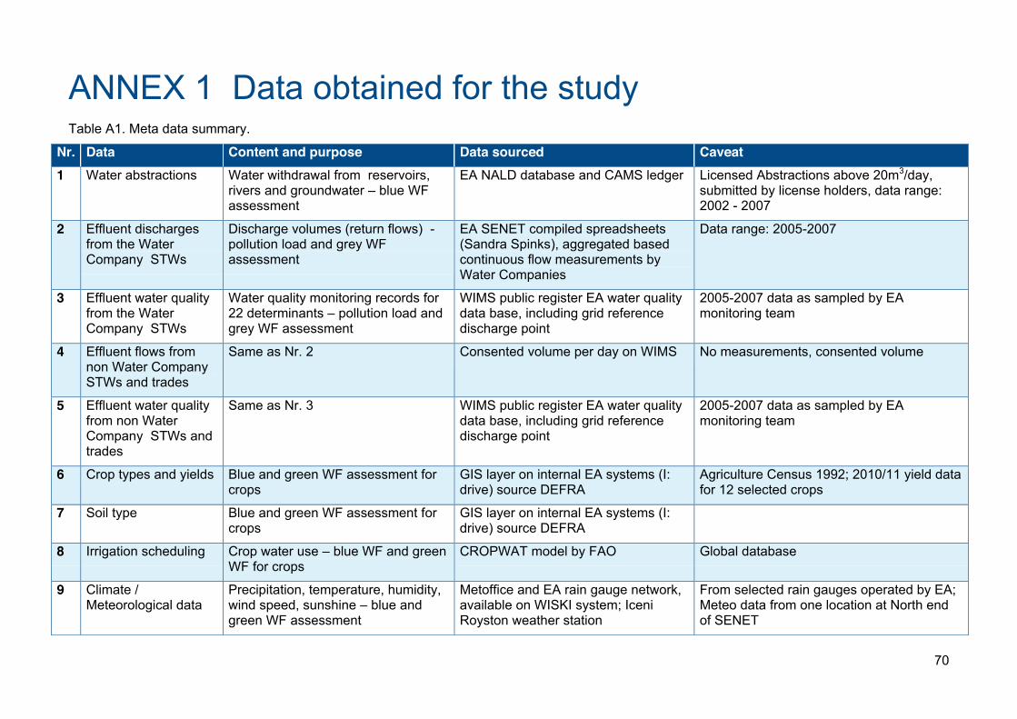
70

ANNEX 1 Data obtained for the study Table A1. Meta data summary.

Nr. Data Content and purpose Data sourced Caveat 1 Water abstractions Water withdrawal from reservoirs,

rivers and groundwater – blue WF assessment

EA NALD database and CAMS ledger Licensed Abstractions above 20m3/day, submitted by license holders, data range: 2002 - 2007

2 Effluent discharges from the Water Company STWs

Discharge volumes (return flows) - pollution load and grey WF assessment

EA SENET compiled spreadsheets (Sandra Spinks), aggregated based continuous flow measurements by Water Companies

Data range: 2005-2007

3 Effluent water quality from the Water Company STWs

Water quality monitoring records for 22 determinants – pollution load and grey WF assessment

WIMS public register EA water quality data base, including grid reference discharge point

2005-2007 data as sampled by EA monitoring team

4 Effluent flows from non Water Company STWs and trades

Same as Nr. 2 Consented volume per day on WIMS No measurements, consented volume

5 Effluent water quality from non Water Company STWs and trades

Same as Nr. 3 WIMS public register EA water quality data base, including grid reference discharge point

2005-2007 data as sampled by EA monitoring team

6 Crop types and yields Blue and green WF assessment for crops

GIS layer on internal EA systems (I: drive) source DEFRA

Agriculture Census 1992; 2010/11 yield data for 12 selected crops

7 Soil type Blue and green WF assessment for crops

GIS layer on internal EA systems (I: drive) source DEFRA

8 Irrigation scheduling Crop water use – blue WF and green WF for crops

CROPWAT model by FAO Global database

9 Climate / Meteorological data

Precipitation, temperature, humidity, wind speed, sunshine – blue and green WF assessment

Metoffice and EA rain gauge network, available on WISKI system; Iceni Royston weather station

From selected rain gauges operated by EA; Meteo data from one location at North end of SENET

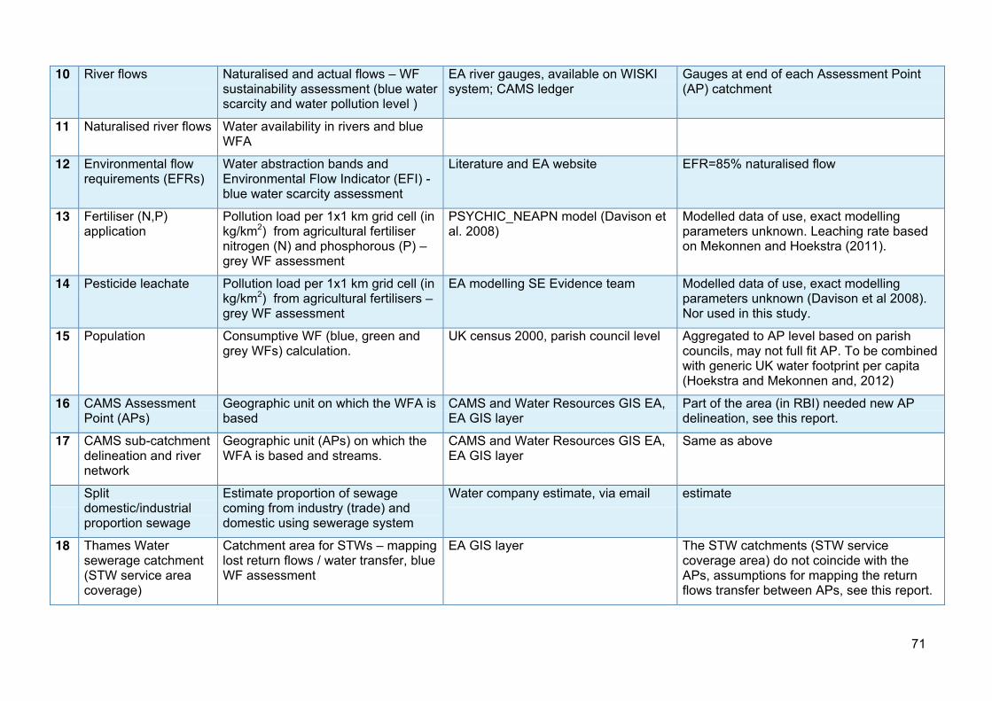
71

10 River flows Naturalised and actual flows – WF sustainability assessment (blue water scarcity and water pollution level )

EA river gauges, available on WISKI system; CAMS ledger

Gauges at end of each Assessment Point (AP) catchment

11 Naturalised river flows Water availability in rivers and blue WFA

12 Environmental flow requirements (EFRs)

Water abstraction bands and Environmental Flow Indicator (EFI) - blue water scarcity assessment

Literature and EA website EFR=85% naturalised flow

13 Fertiliser (N,P) application

Pollution load per 1x1 km grid cell (in kg/km2) from agricultural fertiliser nitrogen (N) and phosphorous (P) – grey WF assessment

PSYCHIC_NEAPN model (Davison et al. 2008)

Modelled data of use, exact modelling parameters unknown. Leaching rate based on Mekonnen and Hoekstra (2011).

14 Pesticide leachate Pollution load per 1x1 km grid cell (in kg/km2) from agricultural fertilisers – grey WF assessment

EA modelling SE Evidence team Modelled data of use, exact modelling parameters unknown (Davison et al 2008). Nor used in this study.

15 Population Consumptive WF (blue, green and grey WFs) calculation.

UK census 2000, parish council level Aggregated to AP level based on parish councils, may not full fit AP. To be combined with generic UK water footprint per capita (Hoekstra and Mekonnen and, 2012)

16 CAMS Assessment Point (APs)

Geographic unit on which the WFA is based

CAMS and Water Resources GIS EA, EA GIS layer

Part of the area (in RBI) needed new AP delineation, see this report.

17 CAMS sub-catchment delineation and river network

Geographic unit (APs) on which the WFA is based and streams.

CAMS and Water Resources GIS EA, EA GIS layer

Same as above

Split domestic/industrial proportion sewage

Estimate proportion of sewage coming from industry (trade) and domestic using sewerage system

Water company estimate, via email estimate

18 Thames Water sewerage catchment (STW service area coverage)

Catchment area for STWs – mapping lost return flows / water transfer, blue WF assessment

EA GIS layer The STW catchments (STW service coverage area) do not coincide with the APs, assumptions for mapping the return flows transfer between APs, see this report.

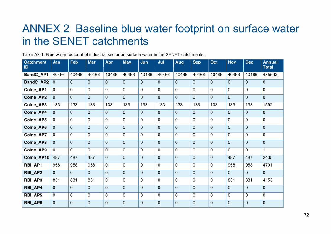
72

ANNEX 2 Baseline blue water footprint on surface water in the SENET catchments Table A2-1. Blue water footprint of industrial sector on surface water in the SENET catchments.

Catchment ID

Jan Feb Mar Apr May Jun Jul Aug Sep Oct Nov Dec Annual Total

BandC_AP1 40466 40466 40466 40466 40466 40466 40466 40466 40466 40466 40466 40466 485592

BandC_AP2 0 0 0 0 0 0 0 0 0 0 0 0 0

Colne_AP1 0 0 0 0 0 0 0 0 0 0 0 0 0

Colne_AP2 0 0 0 0 0 0 0 0 0 0 0 0 0

Colne_AP3 133 133 133 133 133 133 133 133 133 133 133 133 1592

Colne_AP4 0 0 0 0 0 0 0 0 0 0 0 0 0

Colne_AP5 0 0 0 0 0 0 0 0 0 0 0 0 0

Colne_AP6 0 0 0 0 0 0 0 0 0 0 0 0 0

Colne_AP7 0 0 0 0 0 0 0 0 0 0 0 0 0

Colne_AP8 0 0 0 0 0 0 0 0 0 0 0 0 0

Colne_AP9 0 0 0 0 0 0 0 0 0 0 0 0 1

Colne_AP10 487 487 487 0 0 0 0 0 0 0 487 487 2435

RBI_AP1 958 958 958 0 0 0 0 0 0 0 958 958 4791

RBI_AP2 0 0 0 0 0 0 0 0 0 0 0 0 0

RBI_AP3 831 831 831 0 0 0 0 0 0 0 831 831 4153

RBI_AP4 0 0 0 0 0 0 0 0 0 0 0 0 0

RBI_AP5 0 0 0 0 0 0 0 0 0 0 0 0 0

RBI_AP6 0 0 0 0 0 0 0 0 0 0 0 0 0

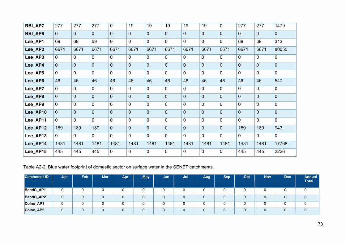
73

RBI_AP7 277 277 277 0 19 19 19 19 19 0 277 277 1479

RBI_AP8 0 0 0 0 0 0 0 0 0 0 0 0 0

Lee_AP1 69 69 69 0 0 0 0 0 0 0 69 69 343

Lee_AP2 6671 6671 6671 6671 6671 6671 6671 6671 6671 6671 6671 6671 80050

Lee_AP3 0 0 0 0 0 0 0 0 0 0 0 0 0

Lee_AP4 0 0 0 0 0 0 0 0 0 0 0 0 0

Lee_AP5 0 0 0 0 0 0 0 0 0 0 0 0 0

Lee_AP6 46 46 46 46 46 46 46 46 46 46 46 46 547

Lee_AP7 0 0 0 0 0 0 0 0 0 0 0 0 0

Lee_AP8 0 0 0 0 0 0 0 0 0 0 0 0 0

Lee_AP9 0 0 0 0 0 0 0 0 0 0 0 0 0

Lee_AP10 0 0 0 0 0 0 0 0 0 0 0 0 0

Lee_AP11 0 0 0 0 0 0 0 0 0 0 0 0 0

Lee_AP12 189 189 189 0 0 0 0 0 0 0 189 189 943

Lee_AP13 0 0 0 0 0 0 0 0 0 0 0 0 0

Lee_AP14 1481 1481 1481 1481 1481 1481 1481 1481 1481 1481 1481 1481 17768

Lee_AP15 445 445 445 0 0 0 0 0 0 0 445 445 2226

Table A2-2. Blue water footprint of domestic sector on surface water in the SENET catchments.

Catchment ID Jan Feb Mar Apr May Jun Jul Aug Sep Oct Nov Dec Annual Total

BandC_AP1 0 0 0 0 0 0 0 0 0 0 0 0 0

BandC_AP2 0 0 0 0 0 0 0 0 0 0 0 0 0

Colne_AP1 0 0 0 0 0 0 0 0 0 0 0 0 0

Colne_AP2 0 0 0 0 0 0 0 0 0 0 0 0 0

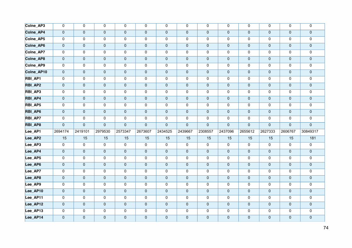
74

Colne_AP3 0 0 0 0 0 0 0 0 0 0 0 0 0

Colne_AP4 0 0 0 0 0 0 0 0 0 0 0 0 0

Colne_AP5 0 0 0 0 0 0 0 0 0 0 0 0 0

Colne_AP6 0 0 0 0 0 0 0 0 0 0 0 0 0

Colne_AP7 0 0 0 0 0 0 0 0 0 0 0 0 0

Colne_AP8 0 0 0 0 0 0 0 0 0 0 0 0 0

Colne_AP9 0 0 0 0 0 0 0 0 0 0 0 0 0

Colne_AP10 0 0 0 0 0 0 0 0 0 0 0 0 0

RBI_AP1 0 0 0 0 0 0 0 0 0 0 0 0 0

RBI_AP2 0 0 0 0 0 0 0 0 0 0 0 0 0

RBI_AP3 0 0 0 0 0 0 0 0 0 0 0 0 0

RBI_AP4 0 0 0 0 0 0 0 0 0 0 0 0 0

RBI_AP5 0 0 0 0 0 0 0 0 0 0 0 0 0

RBI_AP6 0 0 0 0 0 0 0 0 0 0 0 0 0

RBI_AP7 0 0 0 0 0 0 0 0 0 0 0 0 0

RBI_AP8 0 0 0 0 0 0 0 0 0 0 0 0 0

Lee_AP1 2694174 2419101 2979530 2573347 2673607 2434525 2439667 2308557 2437096 2655612 2627333 2606767 30849317

Lee_AP2 15 15 15 15 15 15 15 15 15 15 15 15 181

Lee_AP3 0 0 0 0 0 0 0 0 0 0 0 0 0

Lee_AP4 0 0 0 0 0 0 0 0 0 0 0 0 0

Lee_AP5 0 0 0 0 0 0 0 0 0 0 0 0 0

Lee_AP6 0 0 0 0 0 0 0 0 0 0 0 0 0

Lee_AP7 0 0 0 0 0 0 0 0 0 0 0 0 0

Lee_AP8 0 0 0 0 0 0 0 0 0 0 0 0 0

Lee_AP9 0 0 0 0 0 0 0 0 0 0 0 0 0

Lee_AP10 0 0 0 0 0 0 0 0 0 0 0 0 0

Lee_AP11 0 0 0 0 0 0 0 0 0 0 0 0 0

Lee_AP12 0 0 0 0 0 0 0 0 0 0 0 0 0

Lee_AP13 0 0 0 0 0 0 0 0 0 0 0 0 0

Lee_AP14 0 0 0 0 0 0 0 0 0 0 0 0 0

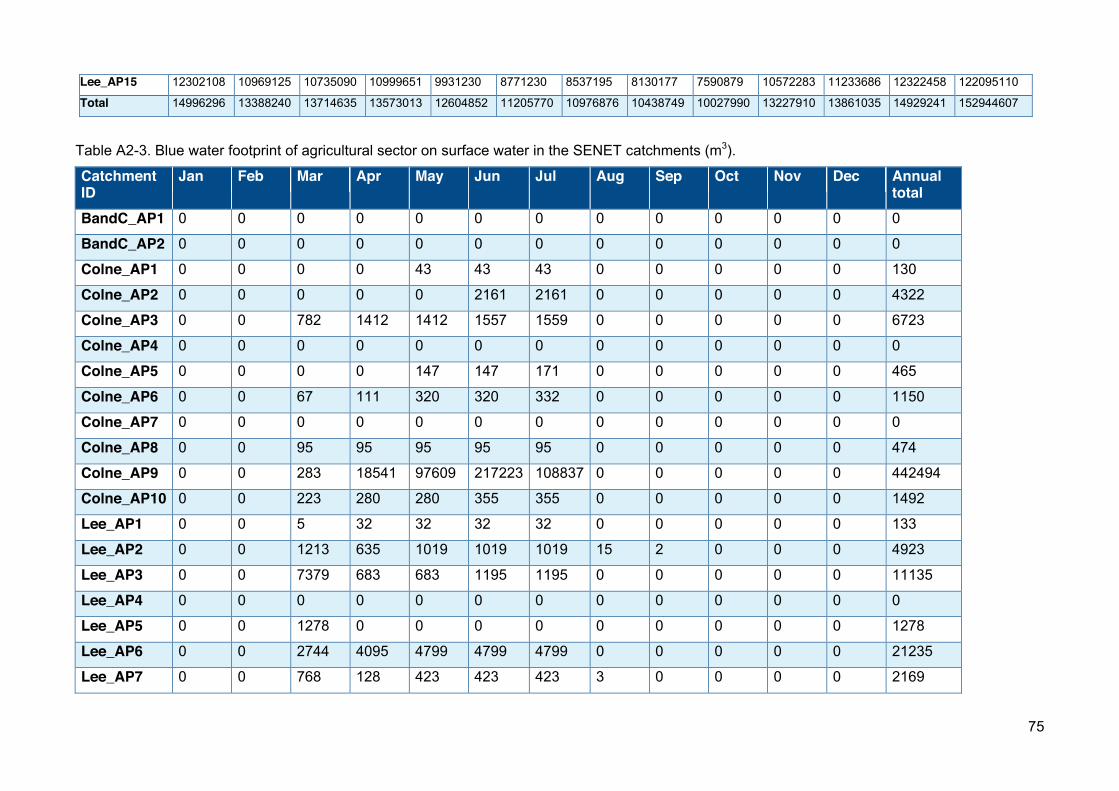
75

Table A2-3. Blue water footprint of agricultural sector on surface water in the SENET catchments (m3).

Catchment ID

Jan Feb Mar Apr May Jun Jul Aug Sep Oct Nov Dec Annual total

BandC_AP1 0 0 0 0 0 0 0 0 0 0 0 0 0

BandC_AP2 0 0 0 0 0 0 0 0 0 0 0 0 0

Colne_AP1 0 0 0 0 43 43 43 0 0 0 0 0 130

Colne_AP2 0 0 0 0 0 2161 2161 0 0 0 0 0 4322

Colne_AP3 0 0 782 1412 1412 1557 1559 0 0 0 0 0 6723

Colne_AP4 0 0 0 0 0 0 0 0 0 0 0 0 0

Colne_AP5 0 0 0 0 147 147 171 0 0 0 0 0 465

Colne_AP6 0 0 67 111 320 320 332 0 0 0 0 0 1150

Colne_AP7 0 0 0 0 0 0 0 0 0 0 0 0 0

Colne_AP8 0 0 95 95 95 95 95 0 0 0 0 0 474

Colne_AP9 0 0 283 18541 97609 217223 108837 0 0 0 0 0 442494

Colne_AP10 0 0 223 280 280 355 355 0 0 0 0 0 1492

Lee_AP1 0 0 5 32 32 32 32 0 0 0 0 0 133

Lee_AP2 0 0 1213 635 1019 1019 1019 15 2 0 0 0 4923

Lee_AP3 0 0 7379 683 683 1195 1195 0 0 0 0 0 11135

Lee_AP4 0 0 0 0 0 0 0 0 0 0 0 0 0

Lee_AP5 0 0 1278 0 0 0 0 0 0 0 0 0 1278

Lee_AP6 0 0 2744 4095 4799 4799 4799 0 0 0 0 0 21235

Lee_AP7 0 0 768 128 423 423 423 3 0 0 0 0 2169

Lee_AP15 12302108 10969125 10735090 10999651 9931230 8771230 8537195 8130177 7590879 10572283 11233686 12322458 122095110

Total 14996296 13388240 13714635 13573013 12604852 11205770 10976876 10438749 10027990 13227910 13861035 14929241 152944607

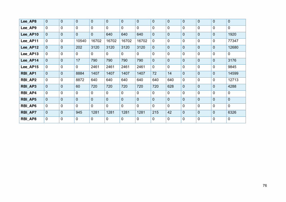
76

Lee_AP8 0 0 0 0 0 0 0 0 0 0 0 0 0

Lee_AP9 0 0 0 0 0 0 0 0 0 0 0 0 0

Lee_AP10 0 0 0 0 640 640 640 0 0 0 0 0 1920

Lee_AP11 0 0 10540 16702 16702 16702 16702 0 0 0 0 0 77347

Lee_AP12 0 0 202 3120 3120 3120 3120 0 0 0 0 0 12680

Lee_AP13 0 0 0 0 0 0 0 0 0 0 0 0 0

Lee_AP14 0 0 17 790 790 790 790 0 0 0 0 0 3176

Lee_AP15 0 0 0 2461 2461 2461 2461 0 0 0 0 0 9845

RBI_AP1 0 0 8884 1407 1407 1407 1407 72 14 0 0 0 14599

RBI_AP2 0 0 8872 640 640 640 640 640 640 0 0 0 12713

RBI_AP3 0 0 60 720 720 720 720 720 628 0 0 0 4288

RBI_AP4 0 0 0 0 0 0 0 0 0 0 0 0 0

RBI_AP5 0 0 0 0 0 0 0 0 0 0 0 0 0

RBI_AP6 0 0 0 0 0 0 0 0 0 0 0 0 0

RBI_AP7 0 0 945 1281 1281 1281 1281 215 42 0 0 0 6326

RBI_AP8 0 0 0 0 0 0 0 0 0 0 0 0 0

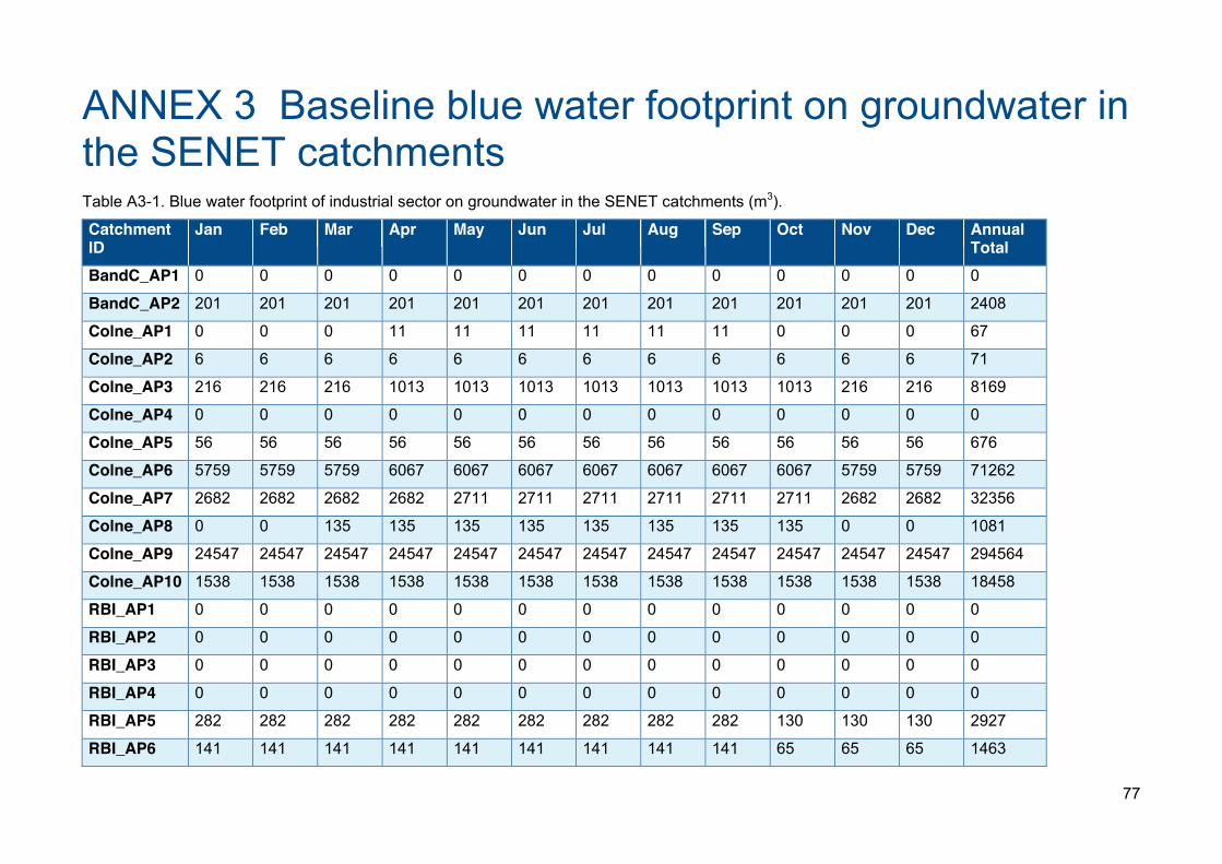
77

ANNEX 3 Baseline blue water footprint on groundwater in the SENET catchments Table A3-1. Blue water footprint of industrial sector on groundwater in the SENET catchments (m3).

Catchment ID

Jan Feb Mar Apr May Jun Jul Aug Sep Oct Nov Dec Annual Total

BandC_AP1 0 0 0 0 0 0 0 0 0 0 0 0 0

BandC_AP2 201 201 201 201 201 201 201 201 201 201 201 201 2408

Colne_AP1 0 0 0 11 11 11 11 11 11 0 0 0 67

Colne_AP2 6 6 6 6 6 6 6 6 6 6 6 6 71

Colne_AP3 216 216 216 1013 1013 1013 1013 1013 1013 1013 216 216 8169

Colne_AP4 0 0 0 0 0 0 0 0 0 0 0 0 0

Colne_AP5 56 56 56 56 56 56 56 56 56 56 56 56 676

Colne_AP6 5759 5759 5759 6067 6067 6067 6067 6067 6067 6067 5759 5759 71262

Colne_AP7 2682 2682 2682 2682 2711 2711 2711 2711 2711 2711 2682 2682 32356

Colne_AP8 0 0 135 135 135 135 135 135 135 135 0 0 1081

Colne_AP9 24547 24547 24547 24547 24547 24547 24547 24547 24547 24547 24547 24547 294564

Colne_AP10 1538 1538 1538 1538 1538 1538 1538 1538 1538 1538 1538 1538 18458

RBI_AP1 0 0 0 0 0 0 0 0 0 0 0 0 0

RBI_AP2 0 0 0 0 0 0 0 0 0 0 0 0 0

RBI_AP3 0 0 0 0 0 0 0 0 0 0 0 0 0

RBI_AP4 0 0 0 0 0 0 0 0 0 0 0 0 0

RBI_AP5 282 282 282 282 282 282 282 282 282 130 130 130 2927

RBI_AP6 141 141 141 141 141 141 141 141 141 65 65 65 1463

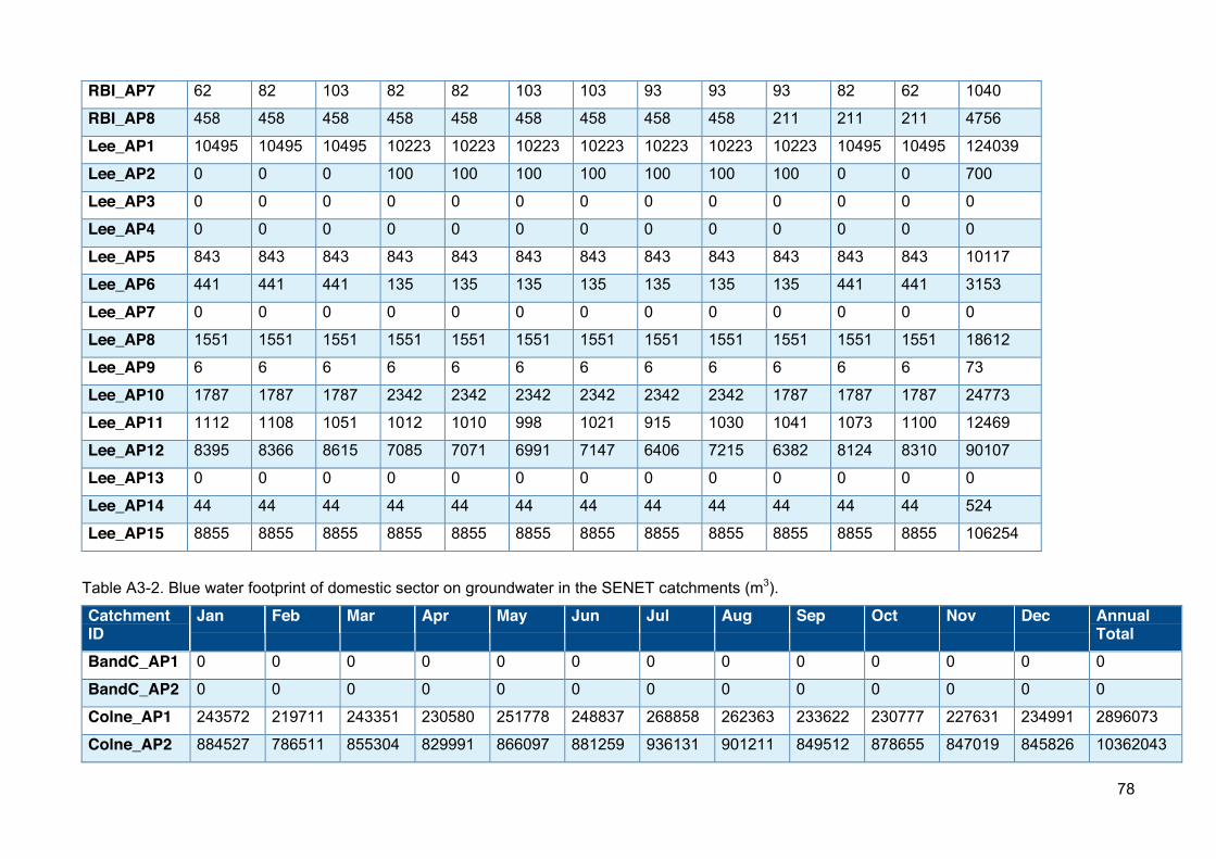
78

RBI_AP7 62 82 103 82 82 103 103 93 93 93 82 62 1040

RBI_AP8 458 458 458 458 458 458 458 458 458 211 211 211 4756

Lee_AP1 10495 10495 10495 10223 10223 10223 10223 10223 10223 10223 10495 10495 124039

Lee_AP2 0 0 0 100 100 100 100 100 100 100 0 0 700

Lee_AP3 0 0 0 0 0 0 0 0 0 0 0 0 0

Lee_AP4 0 0 0 0 0 0 0 0 0 0 0 0 0

Lee_AP5 843 843 843 843 843 843 843 843 843 843 843 843 10117

Lee_AP6 441 441 441 135 135 135 135 135 135 135 441 441 3153

Lee_AP7 0 0 0 0 0 0 0 0 0 0 0 0 0

Lee_AP8 1551 1551 1551 1551 1551 1551 1551 1551 1551 1551 1551 1551 18612

Lee_AP9 6 6 6 6 6 6 6 6 6 6 6 6 73

Lee_AP10 1787 1787 1787 2342 2342 2342 2342 2342 2342 1787 1787 1787 24773

Lee_AP11 1112 1108 1051 1012 1010 998 1021 915 1030 1041 1073 1100 12469

Lee_AP12 8395 8366 8615 7085 7071 6991 7147 6406 7215 6382 8124 8310 90107

Lee_AP13 0 0 0 0 0 0 0 0 0 0 0 0 0

Lee_AP14 44 44 44 44 44 44 44 44 44 44 44 44 524

Lee_AP15 8855 8855 8855 8855 8855 8855 8855 8855 8855 8855 8855 8855 106254

Table A3-2. Blue water footprint of domestic sector on groundwater in the SENET catchments (m3).

Catchment ID

Jan Feb Mar Apr May Jun Jul Aug Sep Oct Nov Dec Annual Total

BandC_AP1 0 0 0 0 0 0 0 0 0 0 0 0 0

BandC_AP2 0 0 0 0 0 0 0 0 0 0 0 0 0

Colne_AP1 243572 219711 243351 230580 251778 248837 268858 262363 233622 230777 227631 234991 2896073

Colne_AP2 884527 786511 855304 829991 866097 881259 936131 901211 849512 878655 847019 845826 10362043

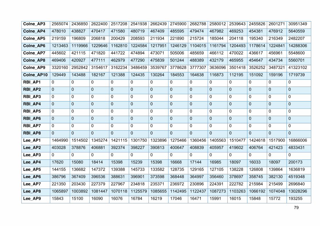
79

Colne_AP3 2565074 2436850 2622400 2517208 2541938 2662439 2745900 2682788 2580012 2539643 2455826 2601271 30951349

Colne_AP4 478010 438827 470417 471580 480719 467409 485595 479474 467982 469253 454381 476912 5640559

Colne_AP5 219159 196809 206818 200429 208593 211934 221890 215724 185044 204118 195340 216349 2482207

Colne_AP6 1213463 1119966 1229646 1162810 1224584 1217951 1246129 1104015 1161794 1204493 1178614 1224841 14288306

Colne_AP7 445602 421115 471820 441722 474894 473071 505006 485659 466112 470022 436617 456961 5548600

Colne_AP8 469406 420927 477111 462979 477290 475839 501244 488389 432179 465955 454647 434734 5560701

Colne_AP9 3320160 2952842 3154617 3162234 3486459 3539767 3778628 3777307 3636096 3501418 3526252 3487321 41323102

Colne_AP10 129449 143488 182167 121388 124435 130264 184553 164638 116873 112195 151092 159196 1719739

RBI_AP1 0 0 0 0 0 0 0 0 0 0 0 0 0

RBI_AP2 0 0 0 0 0 0 0 0 0 0 0 0 0

RBI_AP3 0 0 0 0 0 0 0 0 0 0 0 0 0

RBI_AP4 0 0 0 0 0 0 0 0 0 0 0 0 0

RBI_AP5 0 0 0 0 0 0 0 0 0 0 0 0 0

RBI_AP6 0 0 0 0 0 0 0 0 0 0 0 0 0

RBI_AP7 0 0 0 0 0 0 0 0 0 0 0 0 0

RBI_AP8 0 0 0 0 0 0 0 0 0 0 0 0 0

Lee_AP1 1464990 1514502 1345274 1421115 1301750 1323896 1275466 1360456 1405563 1510477 1424618 1517900 16866006

Lee_AP2 403028 378876 406881 392374 398227 390813 400647 408839 405957 419602 406764 421423 4833431

Lee_AP3 0 0 0 0 0 0 0 0 0 0 0 0 0

Lee_AP4 17620 15080 18414 15398 15239 15398 16668 17144 16985 18097 16033 18097 200173

Lee_AP5 144155 136682 147372 139388 145733 133582 128735 129165 127105 138228 126808 139864 1636819

Lee_AP6 386796 367409 396536 388631 396901 373598 368448 364997 356460 378697 358745 382130 4519348

Lee_AP7 221350 203430 227379 227967 234818 235371 236972 230896 224391 222782 215984 215499 2696840

Lee_AP8 1065897 1003892 1081447 1070118 1125579 1085655 1142495 1122437 1087273 1103263 1066192 1074048 13028296

Lee_AP9 15843 15100 16090 16076 16784 16219 17046 16471 15991 16015 15848 15772 193255

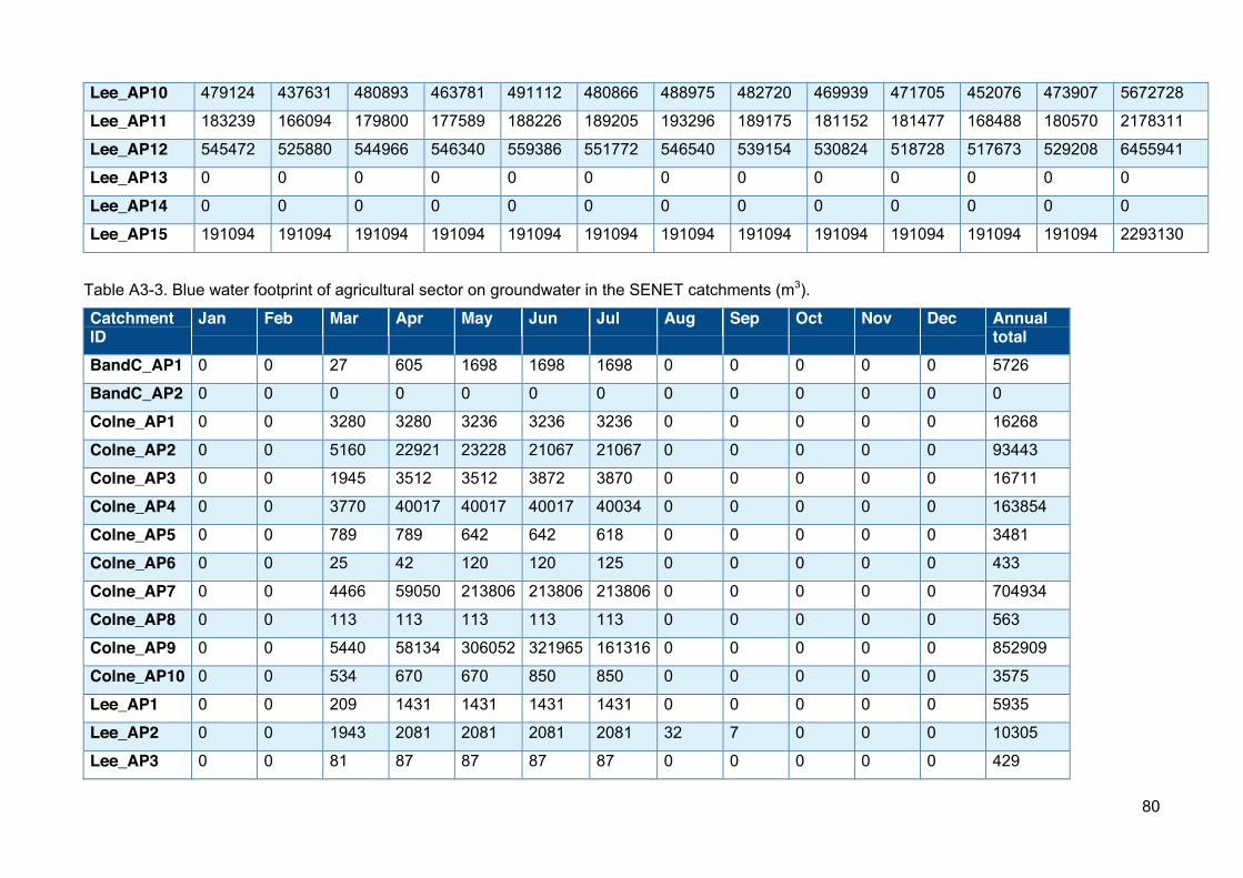
80

Lee_AP10 479124 437631 480893 463781 491112 480866 488975 482720 469939 471705 452076 473907 5672728

Lee_AP11 183239 166094 179800 177589 188226 189205 193296 189175 181152 181477 168488 180570 2178311

Lee_AP12 545472 525880 544966 546340 559386 551772 546540 539154 530824 518728 517673 529208 6455941

Lee_AP13 0 0 0 0 0 0 0 0 0 0 0 0 0

Lee_AP14 0 0 0 0 0 0 0 0 0 0 0 0 0

Lee_AP15 191094 191094 191094 191094 191094 191094 191094 191094 191094 191094 191094 191094 2293130

Table A3-3. Blue water footprint of agricultural sector on groundwater in the SENET catchments (m3).

Catchment ID

Jan Feb Mar Apr May Jun Jul Aug Sep Oct Nov Dec Annual total

BandC_AP1 0 0 27 605 1698 1698 1698 0 0 0 0 0 5726

BandC_AP2 0 0 0 0 0 0 0 0 0 0 0 0 0

Colne_AP1 0 0 3280 3280 3236 3236 3236 0 0 0 0 0 16268

Colne_AP2 0 0 5160 22921 23228 21067 21067 0 0 0 0 0 93443

Colne_AP3 0 0 1945 3512 3512 3872 3870 0 0 0 0 0 16711

Colne_AP4 0 0 3770 40017 40017 40017 40034 0 0 0 0 0 163854

Colne_AP5 0 0 789 789 642 642 618 0 0 0 0 0 3481

Colne_AP6 0 0 25 42 120 120 125 0 0 0 0 0 433

Colne_AP7 0 0 4466 59050 213806 213806 213806 0 0 0 0 0 704934

Colne_AP8 0 0 113 113 113 113 113 0 0 0 0 0 563

Colne_AP9 0 0 5440 58134 306052 321965 161316 0 0 0 0 0 852909

Colne_AP10 0 0 534 670 670 850 850 0 0 0 0 0 3575

Lee_AP1 0 0 209 1431 1431 1431 1431 0 0 0 0 0 5935

Lee_AP2 0 0 1943 2081 2081 2081 2081 32 7 0 0 0 10305

Lee_AP3 0 0 81 87 87 87 87 0 0 0 0 0 429

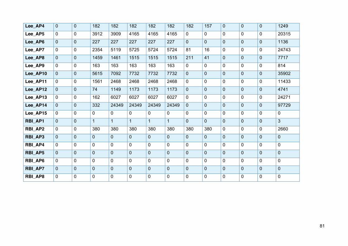
81

Lee_AP4 0 0 182 182 182 182 182 182 157 0 0 0 1249

Lee_AP5 0 0 3912 3909 4165 4165 4165 0 0 0 0 0 20315

Lee_AP6 0 0 227 227 227 227 227 0 0 0 0 0 1136

Lee_AP7 0 0 2354 5119 5725 5724 5724 81 16 0 0 0 24743

Lee_AP8 0 0 1459 1461 1515 1515 1515 211 41 0 0 0 7717

Lee_AP9 0 0 163 163 163 163 163 0 0 0 0 0 814

Lee_AP10 0 0 5615 7092 7732 7732 7732 0 0 0 0 0 35902

Lee_AP11 0 0 1561 2468 2468 2468 2468 0 0 0 0 0 11433

Lee_AP12 0 0 74 1149 1173 1173 1173 0 0 0 0 0 4741

Lee_AP13 0 0 162 6027 6027 6027 6027 0 0 0 0 0 24271

Lee_AP14 0 0 332 24349 24349 24349 24349 0 0 0 0 0 97729

Lee_AP15 0 0 0 0 0 0 0 0 0 0 0 0 0

RBI_AP1 0 0 1 1 1 1 1 0 0 0 0 0 3

RBI_AP2 0 0 380 380 380 380 380 380 380 0 0 0 2660

RBI_AP3 0 0 0 0 0 0 0 0 0 0 0 0 0

RBI_AP4 0 0 0 0 0 0 0 0 0 0 0 0 0

RBI_AP5 0 0 0 0 0 0 0 0 0 0 0 0 0

RBI_AP6 0 0 0 0 0 0 0 0 0 0 0 0 0

RBI_AP7 0 0 0 0 0 0 0 0 0 0 0 0 0

RBI_AP8 0 0 0 0 0 0 0 0 0 0 0 0 0

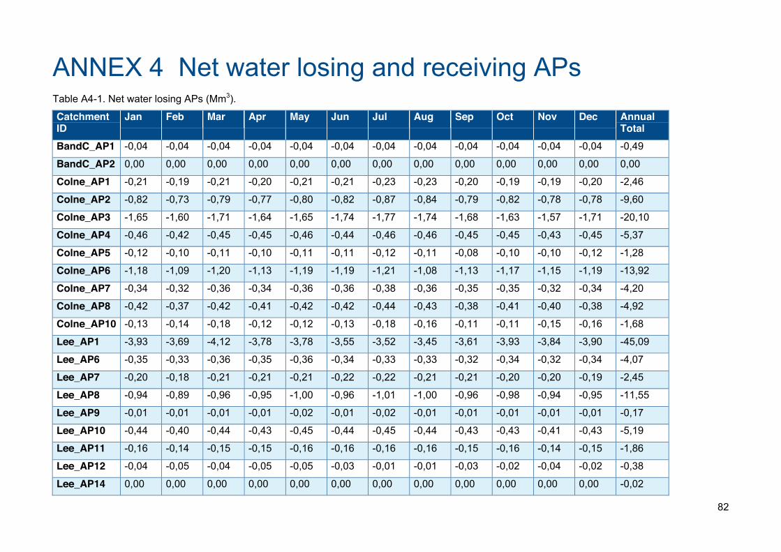
82

ANNEX 4 Net water losing and receiving APs Table A4-1. Net water losing APs (Mm3).

Catchment ID

Jan Feb Mar Apr May Jun Jul Aug Sep Oct Nov Dec Annual Total

BandC_AP1 -0,04 -0,04 -0,04 -0,04 -0,04 -0,04 -0,04 -0,04 -0,04 -0,04 -0,04 -0,04 -0,49

BandC_AP2 0,00 0,00 0,00 0,00 0,00 0,00 0,00 0,00 0,00 0,00 0,00 0,00 0,00

Colne_AP1 -0,21 -0,19 -0,21 -0,20 -0,21 -0,21 -0,23 -0,23 -0,20 -0,19 -0,19 -0,20 -2,46

Colne_AP2 -0,82 -0,73 -0,79 -0,77 -0,80 -0,82 -0,87 -0,84 -0,79 -0,82 -0,78 -0,78 -9,60

Colne_AP3 -1,65 -1,60 -1,71 -1,64 -1,65 -1,74 -1,77 -1,74 -1,68 -1,63 -1,57 -1,71 -20,10

Colne_AP4 -0,46 -0,42 -0,45 -0,45 -0,46 -0,44 -0,46 -0,46 -0,45 -0,45 -0,43 -0,45 -5,37

Colne_AP5 -0,12 -0,10 -0,11 -0,10 -0,11 -0,11 -0,12 -0,11 -0,08 -0,10 -0,10 -0,12 -1,28

Colne_AP6 -1,18 -1,09 -1,20 -1,13 -1,19 -1,19 -1,21 -1,08 -1,13 -1,17 -1,15 -1,19 -13,92

Colne_AP7 -0,34 -0,32 -0,36 -0,34 -0,36 -0,36 -0,38 -0,36 -0,35 -0,35 -0,32 -0,34 -4,20

Colne_AP8 -0,42 -0,37 -0,42 -0,41 -0,42 -0,42 -0,44 -0,43 -0,38 -0,41 -0,40 -0,38 -4,92

Colne_AP10 -0,13 -0,14 -0,18 -0,12 -0,12 -0,13 -0,18 -0,16 -0,11 -0,11 -0,15 -0,16 -1,68

Lee_AP1 -3,93 -3,69 -4,12 -3,78 -3,78 -3,55 -3,52 -3,45 -3,61 -3,93 -3,84 -3,90 -45,09

Lee_AP6 -0,35 -0,33 -0,36 -0,35 -0,36 -0,34 -0,33 -0,33 -0,32 -0,34 -0,32 -0,34 -4,07

Lee_AP7 -0,20 -0,18 -0,21 -0,21 -0,21 -0,22 -0,22 -0,21 -0,21 -0,20 -0,20 -0,19 -2,45

Lee_AP8 -0,94 -0,89 -0,96 -0,95 -1,00 -0,96 -1,01 -1,00 -0,96 -0,98 -0,94 -0,95 -11,55

Lee_AP9 -0,01 -0,01 -0,01 -0,01 -0,02 -0,01 -0,02 -0,01 -0,01 -0,01 -0,01 -0,01 -0,17

Lee_AP10 -0,44 -0,40 -0,44 -0,43 -0,45 -0,44 -0,45 -0,44 -0,43 -0,43 -0,41 -0,43 -5,19

Lee_AP11 -0,16 -0,14 -0,15 -0,15 -0,16 -0,16 -0,16 -0,16 -0,15 -0,16 -0,14 -0,15 -1,86

Lee_AP12 -0,04 -0,05 -0,04 -0,05 -0,05 -0,03 -0,01 -0,01 -0,03 -0,02 -0,04 -0,02 -0,38

Lee_AP14 0,00 0,00 0,00 0,00 0,00 0,00 0,00 0,00 0,00 0,00 0,00 0,00 -0,02

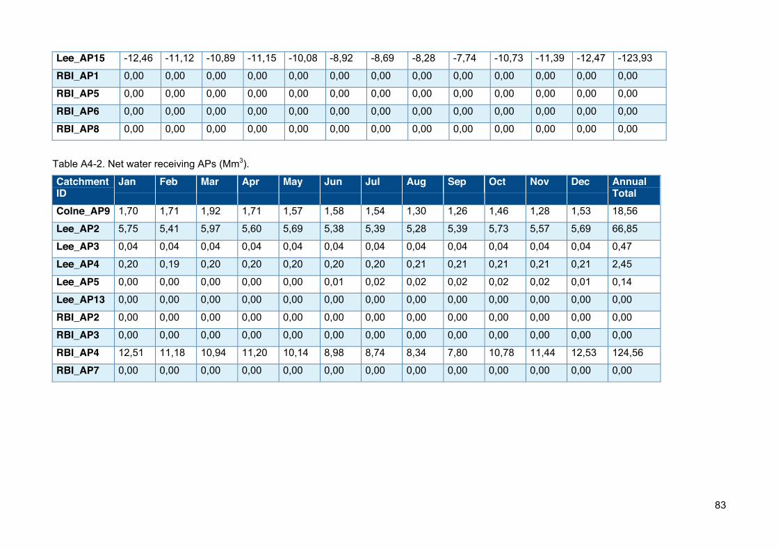
83

Lee_AP15 -12,46 -11,12 -10,89 -11,15 -10,08 -8,92 -8,69 -8,28 -7,74 -10,73 -11,39 -12,47 -123,93

RBI_AP1 0,00 0,00 0,00 0,00 0,00 0,00 0,00 0,00 0,00 0,00 0,00 0,00 0,00

RBI_AP5 0,00 0,00 0,00 0,00 0,00 0,00 0,00 0,00 0,00 0,00 0,00 0,00 0,00

RBI_AP6 0,00 0,00 0,00 0,00 0,00 0,00 0,00 0,00 0,00 0,00 0,00 0,00 0,00

RBI_AP8 0,00 0,00 0,00 0,00 0,00 0,00 0,00 0,00 0,00 0,00 0,00 0,00 0,00

Table A4-2. Net water receiving APs (Mm3).

Catchment ID

Jan Feb Mar Apr May Jun Jul Aug Sep Oct Nov Dec Annual Total

Colne_AP9 1,70 1,71 1,92 1,71 1,57 1,58 1,54 1,30 1,26 1,46 1,28 1,53 18,56

Lee_AP2 5,75 5,41 5,97 5,60 5,69 5,38 5,39 5,28 5,39 5,73 5,57 5,69 66,85

Lee_AP3 0,04 0,04 0,04 0,04 0,04 0,04 0,04 0,04 0,04 0,04 0,04 0,04 0,47

Lee_AP4 0,20 0,19 0,20 0,20 0,20 0,20 0,20 0,21 0,21 0,21 0,21 0,21 2,45

Lee_AP5 0,00 0,00 0,00 0,00 0,00 0,01 0,02 0,02 0,02 0,02 0,02 0,01 0,14

Lee_AP13 0,00 0,00 0,00 0,00 0,00 0,00 0,00 0,00 0,00 0,00 0,00 0,00 0,00

RBI_AP2 0,00 0,00 0,00 0,00 0,00 0,00 0,00 0,00 0,00 0,00 0,00 0,00 0,00

RBI_AP3 0,00 0,00 0,00 0,00 0,00 0,00 0,00 0,00 0,00 0,00 0,00 0,00 0,00

RBI_AP4 12,51 11,18 10,94 11,20 10,14 8,98 8,74 8,34 7,80 10,78 11,44 12,53 124,56

RBI_AP7 0,00 0,00 0,00 0,00 0,00 0,00 0,00 0,00 0,00 0,00 0,00 0,00 0,00

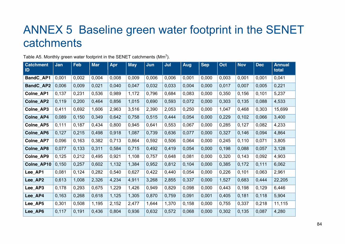
84

ANNEX 5 Baseline green water footprint in the SENET catchments Table A5. Monthly green water footprint in the SENET catchments (Mm3).

Catchment ID

Jan Feb Mar Apr May Jun Jul Aug Sep Oct Nov Dec Annual total

BandC_AP1 0,001 0,002 0,004 0,008 0,009 0,006 0,006 0,001 0,000 0,003 0,001 0,001 0,041

BandC_AP2 0,006 0,009 0,021 0,040 0,047 0,032 0,033 0,004 0,000 0,017 0,007 0,005 0,221

Colne_AP1 0,137 0,231 0,536 0,989 1,172 0,796 0,684 0,083 0,000 0,350 0,156 0,101 5,237

Colne_AP2 0,119 0,200 0,464 0,856 1,015 0,690 0,593 0,072 0,000 0,303 0,135 0,088 4,533

Colne_AP3 0,411 0,692 1,606 2,963 3,516 2,390 2,053 0,250 0,000 1,047 0,468 0,303 15,699

Colne_AP4 0,089 0,150 0,349 0,642 0,758 0,515 0,444 0,054 0,000 0,229 0,102 0,066 3,400

Colne_AP5 0,111 0,187 0,434 0,800 0,945 0,641 0,553 0,067 0,000 0,285 0,127 0,082 4,233

Colne_AP6 0,127 0,215 0,498 0,918 1,087 0,739 0,636 0,077 0,000 0,327 0,146 0,094 4,864

Colne_AP7 0,096 0,163 0,382 0,713 0,864 0,592 0,506 0,064 0,000 0,245 0,110 0,071 3,805

Colne_AP8 0,077 0,133 0,311 0,584 0,715 0,492 0,419 0,054 0,000 0,198 0,088 0,057 3,128

Colne_AP9 0,125 0,212 0,495 0,921 1,108 0,757 0,648 0,081 0,000 0,320 0,143 0,092 4,903

Colne_AP10 0,150 0,257 0,602 1,132 1,384 0,952 0,812 0,104 0,000 0,385 0,172 0,111 6,062

Lee_AP1 0,081 0,124 0,282 0,540 0,627 0,422 0,440 0,054 0,000 0,226 0,101 0,063 2,961

Lee_AP2 0,613 1,008 2,326 4,234 4,911 3,268 2,855 0,337 0,000 1,527 0,683 0,444 22,205

Lee_AP3 0,178 0,293 0,675 1,229 1,426 0,949 0,829 0,098 0,000 0,443 0,198 0,129 6,446

Lee_AP4 0,163 0,268 0,618 1,125 1,305 0,870 0,759 0,091 0,001 0,405 0,181 0,118 5,904

Lee_AP5 0,301 0,508 1,195 2,152 2,477 1,644 1,370 0,158 0,000 0,755 0,337 0,218 11,115

Lee_AP6 0,117 0,191 0,436 0,804 0,936 0,632 0,572 0,068 0,000 0,302 0,135 0,087 4,280

85

Lee_AP7 0,466 0,763 1,744 3,214 3,744 2,527 2,286 0,272 0,000 1,207 0,539 0,348 17,113

Lee_AP8 0,468 0,789 1,842 3,362 3,915 2,645 2,262 0,267 0,000 1,210 0,540 0,348 17,648

Lee_AP9 0,122 0,205 0,479 0,874 1,018 0,688 0,588 0,069 0,000 0,315 0,140 0,090 4,589

Lee_AP10 0,126 0,215 0,507 0,932 1,097 0,744 0,631 0,076 0,000 0,329 0,147 0,094 4,898

Lee_AP11 0,275 0,468 1,103 2,027 2,387 1,619 1,376 0,165 0,000 0,717 0,320 0,205 10,661

Lee_AP12 0,110 0,169 0,384 0,736 0,856 0,576 0,601 0,073 0,000 0,307 0,137 0,086 4,035

Lee_AP13 0,092 0,142 0,322 0,617 0,717 0,482 0,505 0,062 0,000 0,259 0,115 0,072 3,385

Lee_AP14 0,174 0,268 0,607 1,162 1,349 0,907 0,950 0,116 0,000 0,487 0,217 0,136 6,372

Lee_AP15 0,019 0,029 0,066 0,127 0,148 0,099 0,105 0,013 0,000 0,054 0,024 0,015 0,699

RBI_AP1 0,254 0,428 1,035 1,832 2,102 1,339 1,037 0,119 0,000 0,573 0,256 0,168 9,144

RBI_AP2 0,499 0,819 1,903 3,469 4,005 2,655 2,322 0,316 0,029 1,236 0,553 0,359 18,164

RBI_AP3 0,360 0,605 1,389 2,486 2,861 1,918 1,590 0,187 0,003 0,883 0,395 0,260 12,938

RBI_AP4 0,036 0,060 0,138 0,248 0,286 0,192 0,163 0,019 0,000 0,090 0,040 0,026 1,299

RBI_AP5 0,003 0,005 0,011 0,020 0,023 0,015 0,014 0,002 0,000 0,008 0,003 0,002 0,105

RBI_AP6 0,034 0,053 0,121 0,230 0,267 0,179 0,184 0,022 0,000 0,095 0,042 0,027 1,256

RBI_AP7 0,091 0,152 0,359 0,649 0,747 0,489 0,416 0,049 0,000 0,226 0,101 0,065 3,344

RBI_AP8 0,004 0,006 0,014 0,027 0,031 0,021 0,022 0,003 0,000 0,011 0,005 0,003 0,147

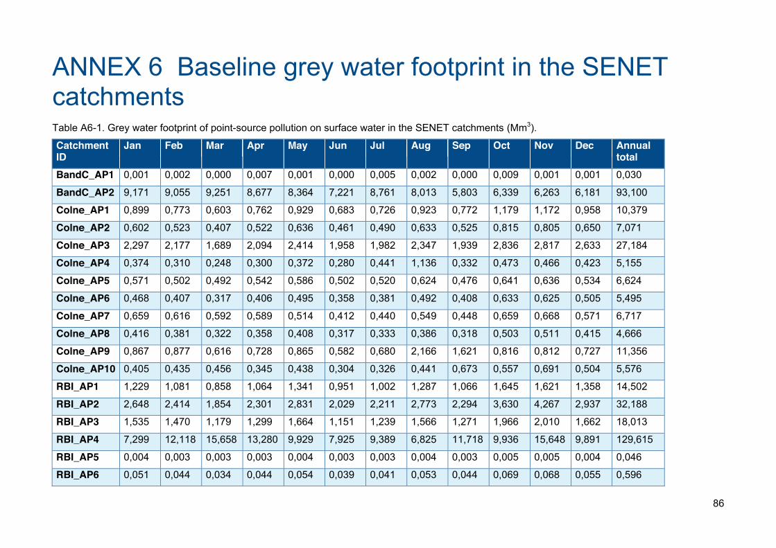
86

ANNEX 6 Baseline grey water footprint in the SENET catchments Table A6-1. Grey water footprint of point-source pollution on surface water in the SENET catchments (Mm3).

Catchment ID

Jan Feb Mar Apr May Jun Jul Aug Sep Oct Nov Dec Annual total

BandC_AP1 0,001 0,002 0,000 0,007 0,001 0,000 0,005 0,002 0,000 0,009 0,001 0,001 0,030

BandC_AP2 9,171 9,055 9,251 8,677 8,364 7,221 8,761 8,013 5,803 6,339 6,263 6,181 93,100

Colne_AP1 0,899 0,773 0,603 0,762 0,929 0,683 0,726 0,923 0,772 1,179 1,172 0,958 10,379

Colne_AP2 0,602 0,523 0,407 0,522 0,636 0,461 0,490 0,633 0,525 0,815 0,805 0,650 7,071

Colne_AP3 2,297 2,177 1,689 2,094 2,414 1,958 1,982 2,347 1,939 2,836 2,817 2,633 27,184

Colne_AP4 0,374 0,310 0,248 0,300 0,372 0,280 0,441 1,136 0,332 0,473 0,466 0,423 5,155

Colne_AP5 0,571 0,502 0,492 0,542 0,586 0,502 0,520 0,624 0,476 0,641 0,636 0,534 6,624

Colne_AP6 0,468 0,407 0,317 0,406 0,495 0,358 0,381 0,492 0,408 0,633 0,625 0,505 5,495

Colne_AP7 0,659 0,616 0,592 0,589 0,514 0,412 0,440 0,549 0,448 0,659 0,668 0,571 6,717

Colne_AP8 0,416 0,381 0,322 0,358 0,408 0,317 0,333 0,386 0,318 0,503 0,511 0,415 4,666

Colne_AP9 0,867 0,877 0,616 0,728 0,865 0,582 0,680 2,166 1,621 0,816 0,812 0,727 11,356

Colne_AP10 0,405 0,435 0,456 0,345 0,438 0,304 0,326 0,441 0,673 0,557 0,691 0,504 5,576

RBI_AP1 1,229 1,081 0,858 1,064 1,341 0,951 1,002 1,287 1,066 1,645 1,621 1,358 14,502

RBI_AP2 2,648 2,414 1,854 2,301 2,831 2,029 2,211 2,773 2,294 3,630 4,267 2,937 32,188

RBI_AP3 1,535 1,470 1,179 1,299 1,664 1,151 1,239 1,566 1,271 1,966 2,010 1,662 18,013

RBI_AP4 7,299 12,118 15,658 13,280 9,929 7,925 9,389 6,825 11,718 9,936 15,648 9,891 129,615

RBI_AP5 0,004 0,003 0,003 0,003 0,004 0,003 0,003 0,004 0,003 0,005 0,005 0,004 0,046

RBI_AP6 0,051 0,044 0,034 0,044 0,054 0,039 0,041 0,053 0,044 0,069 0,068 0,055 0,596

87

RBI_AP7 2,439 3,779 3,529 2,191 3,257 3,181 3,937 4,313 3,582 4,006 2,418 3,584 40,216

RBI_AP8 0,002 0,002 0,002 0,002 0,002 0,002 0,002 0,002 0,002 0,003 0,003 0,002 0,027

Lee_AP1 0,181 0,155 0,120 0,157 0,188 0,135 0,147 0,186 0,154 0,239 0,236 0,191 2,089

Lee_AP2 3,470 2,981 2,455 2,771 3,427 2,411 2,568 3,239 2,677 3,950 3,941 3,295 37,187

Lee_AP3 0,931 0,810 0,652 0,804 1,157 0,690 0,726 0,928 1,001 1,206 1,186 0,976 11,066

Lee_AP4 0,885 0,771 0,593 0,759 0,930 0,665 0,716 0,919 0,762 1,182 1,170 0,938 10,291

Lee_AP5 1,429 1,204 1,037 1,202 1,461 1,059 1,207 1,467 1,204 1,881 1,930 1,493 16,573

Lee_AP6 0,710 0,427 0,330 0,644 0,515 0,373 0,563 0,576 0,536 0,772 0,651 0,526 6,623

Lee_AP7 2,654 2,277 1,778 2,294 2,720 2,035 2,160 2,752 2,249 3,465 3,478 2,751 30,612

Lee_AP8 2,324 2,005 1,562 2,026 2,430 1,763 1,879 2,422 2,009 3,126 3,088 2,481 27,113

Lee_AP9 0,359 0,312 0,243 0,311 0,379 0,275 0,292 0,377 0,313 0,486 0,480 0,388 4,216

Lee_AP10 0,403 0,350 0,273 0,350 0,426 0,309 0,328 0,424 0,352 0,546 0,539 0,436 4,736

Lee_AP11 1,606 1,396 1,089 1,396 1,698 1,233 1,591 1,678 1,396 2,161 2,137 1,732 19,113

Lee_AP12 0,618 0,493 0,501 0,551 0,554 0,520 0,444 0,522 0,466 0,660 0,632 0,603 6,565

Lee_AP13 0,279 0,243 0,189 0,242 0,295 0,214 0,227 0,294 0,243 0,378 0,373 0,302 3,278

Lee_AP14 0,755 0,531 0,378 0,774 0,500 0,497 0,596 0,942 0,524 1,406 0,632 0,675 8,209

Lee_AP15 12,693 10,824 11,605 3,628 3,845 10,107 11,289 11,030 9,322 3,144 14,725 3,625 105,836

Table A6-2. Grey water footprint of point-source pollution on groundwater in the SENET catchments (Mm3).

Catchment ID

Jan Feb Mar Apr May Jun Jul Aug Sep Oct Nov Dec Annual total

BandC_AP1 0,269 0,269 0,269 0,269 0,269 0,269 0,269 0,269 0,269 0,269 0,269 0,269 3,226

BandC_AP2 0,020 0,020 0,020 0,020 0,020 0,020 0,020 0,020 0,020 0,020 0,020 0,020 0,240

Colne_AP1 1,348 1,348 1,348 1,348 1,348 1,348 1,348 1,348 1,348 1,348 1,348 1,348 16,178

Colne_AP10 0,056 0,056 0,056 0,056 0,056 0,056 0,056 0,056 0,056 0,056 0,056 0,056 0,672

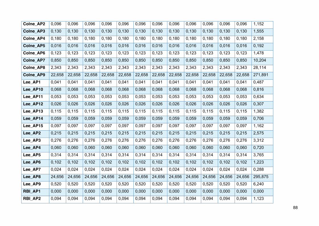
88

Colne_AP2 0,096 0,096 0,096 0,096 0,096 0,096 0,096 0,096 0,096 0,096 0,096 0,096 1,152

Colne_AP3 0,130 0,130 0,130 0,130 0,130 0,130 0,130 0,130 0,130 0,130 0,130 0,130 1,555

Colne_AP4 0,180 0,180 0,180 0,180 0,180 0,180 0,180 0,180 0,180 0,180 0,180 0,180 2,158

Colne_AP5 0,016 0,016 0,016 0,016 0,016 0,016 0,016 0,016 0,016 0,016 0,016 0,016 0,192

Colne_AP6 0,123 0,123 0,123 0,123 0,123 0,123 0,123 0,123 0,123 0,123 0,123 0,123 1,478

Colne_AP7 0,850 0,850 0,850 0,850 0,850 0,850 0,850 0,850 0,850 0,850 0,850 0,850 10,204

Colne_AP8 2,343 2,343 2,343 2,343 2,343 2,343 2,343 2,343 2,343 2,343 2,343 2,343 28,114

Colne_AP9 22,658 22,658 22,658 22,658 22,658 22,658 22,658 22,658 22,658 22,658 22,658 22,658 271,891

Lee_AP1 0,041 0,041 0,041 0,041 0,041 0,041 0,041 0,041 0,041 0,041 0,041 0,041 0,487

Lee_AP10 0,068 0,068 0,068 0,068 0,068 0,068 0,068 0,068 0,068 0,068 0,068 0,068 0,816

Lee_AP11 0,053 0,053 0,053 0,053 0,053 0,053 0,053 0,053 0,053 0,053 0,053 0,053 0,634

Lee_AP12 0,026 0,026 0,026 0,026 0,026 0,026 0,026 0,026 0,026 0,026 0,026 0,026 0,307

Lee_AP13 0,115 0,115 0,115 0,115 0,115 0,115 0,115 0,115 0,115 0,115 0,115 0,115 1,382

Lee_AP14 0,059 0,059 0,059 0,059 0,059 0,059 0,059 0,059 0,059 0,059 0,059 0,059 0,706

Lee_AP15 0,097 0,097 0,097 0,097 0,097 0,097 0,097 0,097 0,097 0,097 0,097 0,097 1,162

Lee_AP2 0,215 0,215 0,215 0,215 0,215 0,215 0,215 0,215 0,215 0,215 0,215 0,215 2,575

Lee_AP3 0,276 0,276 0,276 0,276 0,276 0,276 0,276 0,276 0,276 0,276 0,276 0,276 3,312

Lee_AP4 0,060 0,060 0,060 0,060 0,060 0,060 0,060 0,060 0,060 0,060 0,060 0,060 0,720

Lee_AP5 0,314 0,314 0,314 0,314 0,314 0,314 0,314 0,314 0,314 0,314 0,314 0,314 3,765

Lee_AP6 0,102 0,102 0,102 0,102 0,102 0,102 0,102 0,102 0,102 0,102 0,102 0,102 1,223

Lee_AP7 0,024 0,024 0,024 0,024 0,024 0,024 0,024 0,024 0,024 0,024 0,024 0,024 0,288

Lee_AP8 24,656 24,656 24,656 24,656 24,656 24,656 24,656 24,656 24,656 24,656 24,656 24,656 295,875

Lee_AP9 0,520 0,520 0,520 0,520 0,520 0,520 0,520 0,520 0,520 0,520 0,520 0,520 6,240

RBI_AP1 0,000 0,000 0,000 0,000 0,000 0,000 0,000 0,000 0,000 0,000 0,000 0,000 0,000

RBI_AP2 0,094 0,094 0,094 0,094 0,094 0,094 0,094 0,094 0,094 0,094 0,094 0,094 1,123

89

RBI_AP3 0,516 0,516 0,516 0,516 0,516 0,516 0,516 0,516 0,516 0,516 0,516 0,516 6,192

RBI_AP4 0,000 0,000 0,000 0,000 0,000 0,000 0,000 0,000 0,000 0,000 0,000 0,000 0,000

RBI_AP5 0,000 0,000 0,000 0,000 0,000 0,000 0,000 0,000 0,000 0,000 0,000 0,000 0,000

RBI_AP6 0,000 0,000 0,000 0,000 0,000 0,000 0,000 0,000 0,000 0,000 0,000 0,000 0,000

RBI_AP7 0,016 0,016 0,016 0,016 0,016 0,016 0,016 0,016 0,016 0,016 0,016 0,016 0,192

RBI_AP8 0,000 0,000 0,000 0,000 0,000 0,000 0,000 0,000 0,000 0,000 0,000 0,000 0,000

Table A6-3. Grey water footprint of non-point source pollution on groundwater in the SENET catchments (Mm3).

Catchment_ID Jan Feb Mar Apr Mei Jun Jul Aug Sep Oct. Nov Dec Annual total

BandC_AP1 0,001 0,000 0,000 0,000 0,001 0,000 0,000 0,001 0,000 0,001 0,001 0,001 0,006

BandC_AP2 0,003 0,003 0,002 0,003 0,003 0,002 0,003 0,003 0,003 0,004 0,004 0,003 0,037

Colne_AP1 0,833 0,724 0,564 0,723 0,881 0,638 0,678 0,876 0,726 1,128 1,113 0,900 9,783

Colne_AP10 0,341 0,296 0,231 0,296 0,360 0,261 0,278 0,358 0,297 0,461 0,455 0,368 4,003

Colne_AP2 0,602 0,523 0,407 0,522 0,636 0,461 0,490 0,633 0,525 0,815 0,805 0,650 7,071

Colne_AP3 1,713 1,488 1,159 1,486 1,810 1,311 1,395 1,801 1,493 2,318 2,289 1,850 20,113

Colne_AP4 0,325 0,283 0,220 0,282 0,344 0,249 0,265 0,342 0,284 0,440 0,435 0,351 3,821

Colne_AP5 0,434 0,377 0,293 0,376 0,458 0,332 0,353 0,456 0,378 0,587 0,579 0,468 5,089

Colne_AP6 0,468 0,407 0,317 0,406 0,495 0,358 0,381 0,492 0,408 0,633 0,625 0,505 5,495

Colne_AP7 0,427 0,371 0,289 0,370 0,451 0,327 0,348 0,449 0,372 0,578 0,570 0,461 5,013

Colne_AP8 0,338 0,294 0,229 0,293 0,357 0,259 0,275 0,355 0,295 0,458 0,452 0,365 3,970

Colne_AP9 0,306 0,266 0,207 0,265 0,323 0,234 0,249 0,321 0,266 0,414 0,408 0,330 3,590

Lee_AP1 0,177 0,154 0,120 0,153 0,187 0,135 0,144 0,186 0,154 0,239 0,236 0,191 2,076

Lee_AP10 0,403 0,350 0,273 0,350 0,426 0,309 0,328 0,424 0,352 0,546 0,539 0,436 4,736

Lee_AP11 1,587 1,379 1,074 1,377 1,677 1,215 1,292 1,669 1,383 2,148 2,120 1,714 18,635

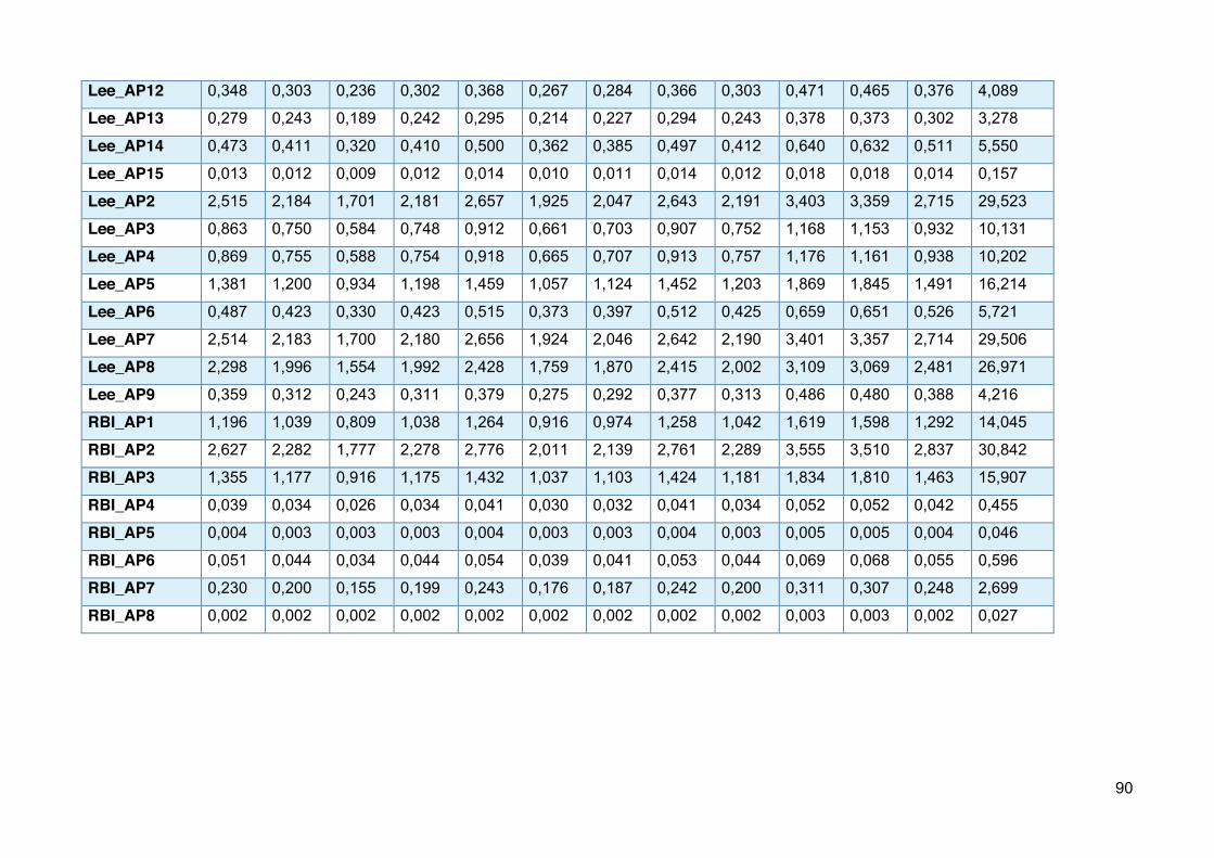
90

Lee_AP12 0,348 0,303 0,236 0,302 0,368 0,267 0,284 0,366 0,303 0,471 0,465 0,376 4,089

Lee_AP13 0,279 0,243 0,189 0,242 0,295 0,214 0,227 0,294 0,243 0,378 0,373 0,302 3,278

Lee_AP14 0,473 0,411 0,320 0,410 0,500 0,362 0,385 0,497 0,412 0,640 0,632 0,511 5,550

Lee_AP15 0,013 0,012 0,009 0,012 0,014 0,010 0,011 0,014 0,012 0,018 0,018 0,014 0,157

Lee_AP2 2,515 2,184 1,701 2,181 2,657 1,925 2,047 2,643 2,191 3,403 3,359 2,715 29,523

Lee_AP3 0,863 0,750 0,584 0,748 0,912 0,661 0,703 0,907 0,752 1,168 1,153 0,932 10,131

Lee_AP4 0,869 0,755 0,588 0,754 0,918 0,665 0,707 0,913 0,757 1,176 1,161 0,938 10,202

Lee_AP5 1,381 1,200 0,934 1,198 1,459 1,057 1,124 1,452 1,203 1,869 1,845 1,491 16,214

Lee_AP6 0,487 0,423 0,330 0,423 0,515 0,373 0,397 0,512 0,425 0,659 0,651 0,526 5,721

Lee_AP7 2,514 2,183 1,700 2,180 2,656 1,924 2,046 2,642 2,190 3,401 3,357 2,714 29,506

Lee_AP8 2,298 1,996 1,554 1,992 2,428 1,759 1,870 2,415 2,002 3,109 3,069 2,481 26,971

Lee_AP9 0,359 0,312 0,243 0,311 0,379 0,275 0,292 0,377 0,313 0,486 0,480 0,388 4,216

RBI_AP1 1,196 1,039 0,809 1,038 1,264 0,916 0,974 1,258 1,042 1,619 1,598 1,292 14,045

RBI_AP2 2,627 2,282 1,777 2,278 2,776 2,011 2,139 2,761 2,289 3,555 3,510 2,837 30,842

RBI_AP3 1,355 1,177 0,916 1,175 1,432 1,037 1,103 1,424 1,181 1,834 1,810 1,463 15,907

RBI_AP4 0,039 0,034 0,026 0,034 0,041 0,030 0,032 0,041 0,034 0,052 0,052 0,042 0,455

RBI_AP5 0,004 0,003 0,003 0,003 0,004 0,003 0,003 0,004 0,003 0,005 0,005 0,004 0,046

RBI_AP6 0,051 0,044 0,034 0,044 0,054 0,039 0,041 0,053 0,044 0,069 0,068 0,055 0,596

RBI_AP7 0,230 0,200 0,155 0,199 0,243 0,176 0,187 0,242 0,200 0,311 0,307 0,248 2,699

RBI_AP8 0,002 0,002 0,002 0,002 0,002 0,002 0,002 0,002 0,002 0,003 0,003 0,002 0,027

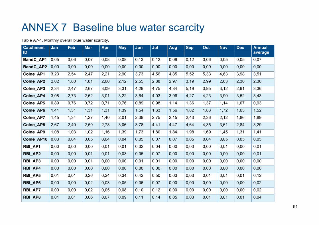
91

ANNEX 7 Baseline blue water scarcity Table A7-1. Monthly overall blue water scarcity.

Catchment ID

Jan Feb Mar Apr May Jun Jul Aug Sep Oct Nov Dec Annual average

BandC_AP1 0,05 0,06 0,07 0,08 0,08 0,13 0,12 0,09 0,12 0,06 0,05 0,05 0,07

BandC_AP2 0,00 0,00 0,00 0,00 0,00 0,00 0,00 0,00 0,00 0,00 0,00 0,00 0,00

Colne_AP1 3,23 2,54 2,47 2,21 2,90 3,73 4,56 4,85 5,52 5,33 4,63 3,98 3,51

Colne_AP2 2,02 1,80 1,81 2,00 2,12 2,55 2,88 2,97 3,19 2,99 2,63 2,30 2,36

Colne_AP3 2,34 2,47 2,67 3,09 3,31 4,29 4,75 4,84 5,19 3,95 3,12 2,91 3,36

Colne_AP4 3,08 2,73 2,62 3,01 3,22 3,64 4,03 3,96 4,27 4,23 3,90 3,52 3,43

Colne_AP5 0,89 0,76 0,72 0,71 0,76 0,89 0,98 1,14 1,36 1,37 1,14 1,07 0,93

Colne_AP6 1,41 1,31 1,31 1,31 1,39 1,54 1,63 1,56 1,82 1,83 1,72 1,63 1,52

Colne_AP7 1,45 1,34 1,27 1,40 2,01 2,39 2,75 2,15 2,43 2,36 2,12 1,86 1,89

Colne_AP8 2,67 2,40 2,50 2,78 3,06 3,78 4,41 4,47 4,64 4,35 3,61 2,84 3,29

Colne_AP9 1,08 1,03 1,02 1,16 1,39 1,73 1,80 1,84 1,98 1,69 1,45 1,31 1,41

Colne_AP10 0,03 0,04 0,05 0,04 0,04 0,05 0,07 0,07 0,05 0,04 0,05 0,05 0,05

RBI_AP1 0,00 0,00 0,00 0,01 0,01 0,02 0,04 0,00 0,00 0,00 0,01 0,00 0,01

RBI_AP2 0,00 0,00 0,01 0,01 0,03 0,05 0,07 0,00 0,00 0,00 0,00 0,00 0,01

RBI_AP3 0,00 0,00 0,01 0,00 0,00 0,01 0,01 0,00 0,00 0,00 0,00 0,00 0,00

RBI_AP4 0,00 0,00 0,00 0,00 0,00 0,00 0,00 0,00 0,00 0,00 0,00 0,00 0,00

RBI_AP5 0,01 0,01 0,26 0,24 0,34 0,42 0,50 0,03 0,03 0,01 0,01 0,01 0,12

RBI_AP6 0,00 0,00 0,02 0,03 0,05 0,06 0,07 0,00 0,00 0,00 0,00 0,00 0,02

RBI_AP7 0,00 0,00 0,02 0,05 0,08 0,10 0,12 0,00 0,00 0,00 0,00 0,00 0,02

RBI_AP8 0,01 0,01 0,06 0,07 0,09 0,11 0,14 0,05 0,03 0,01 0,01 0,01 0,04

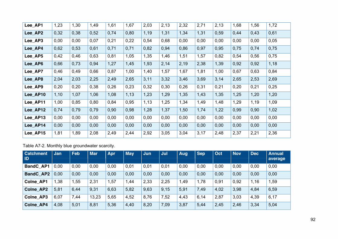
92

Lee_AP1 1,23 1,30 1,49 1,61 1,67 2,03 2,13 2,32 2,71 2,13 1,68 1,56 1,72

Lee_AP2 0,32 0,38 0,52 0,74 0,80 1,19 1,31 1,34 1,31 0,59 0,44 0,43 0,61

Lee_AP3 0,00 0,00 0,07 0,21 0,22 0,54 0,68 0,00 0,00 0,00 0,00 0,00 0,05

Lee_AP4 0,62 0,53 0,61 0,71 0,71 0,82 0,94 0,86 0,97 0,95 0,75 0,74 0,75

Lee_AP5 0,42 0,46 0,63 0,81 1,05 1,35 1,46 1,51 1,57 0,82 0,54 0,56 0,75

Lee_AP6 0,66 0,73 0,94 1,27 1,45 1,93 2,14 2,19 2,38 1,39 0,92 0,92 1,18

Lee_AP7 0,46 0,49 0,66 0,87 1,00 1,40 1,57 1,67 1,81 1,00 0,67 0,63 0,84

Lee_AP8 2,04 2,03 2,25 2,49 2,65 3,11 3,32 3,46 3,69 3,14 2,65 2,53 2,69

Lee_AP9 0,20 0,20 0,38 0,26 0,23 0,32 0,30 0,26 0,31 0,21 0,20 0,21 0,25

Lee_AP10 1,10 1,07 1,06 1,08 1,13 1,23 1,29 1,35 1,43 1,35 1,25 1,20 1,20

Lee_AP11 1,00 0,85 0,80 0,84 0,95 1,13 1,25 1,34 1,49 1,48 1,29 1,19 1,09

Lee_AP12 0,74 0,79 0,79 0,90 0,98 1,28 1,37 1,50 1,74 1,22 0,99 0,90 1,02

Lee_AP13 0,00 0,00 0,00 0,00 0,00 0,00 0,00 0,00 0,00 0,00 0,00 0,00 0,00

Lee_AP14 0,00 0,00 0,00 0,00 0,00 0,00 0,00 0,00 0,00 0,00 0,00 0,00 0,00

Lee_AP15 1,81 1,89 2,08 2,49 2,44 2,92 3,05 3,04 3,17 2,48 2,37 2,21 2,36

Table A7-2. Monthly blue groundwater scarcity.

Catchment ID

Jan Feb Mar Apr May Jun Jul Aug Sep Oct Nov Dec Annual average

BandC_AP1 0,00 0,00 0,00 0,00 0,01 0,01 0,01 0,00 0,00 0,00 0,00 0,00 0,00

BandC_AP2 0,00 0,00 0,00 0,00 0,00 0,00 0,00 0,00 0,00 0,00 0,00 0,00 0,00

Colne_AP1 1,38 1,55 2,31 1,57 1,44 2,33 2,25 1,49 1,78 0,91 0,92 1,16 1,59

Colne_AP2 5,81 6,44 9,31 6,63 5,82 9,63 9,15 5,91 7,49 4,02 3,98 4,84 6,59

Colne_AP3 6,07 7,44 13,23 5,65 4,52 8,76 7,52 4,43 6,14 2,87 3,03 4,39 6,17

Colne_AP4 4,08 5,01 8,81 5,36 4,40 8,20 7,09 3,87 5,44 2,45 2,46 3,34 5,04

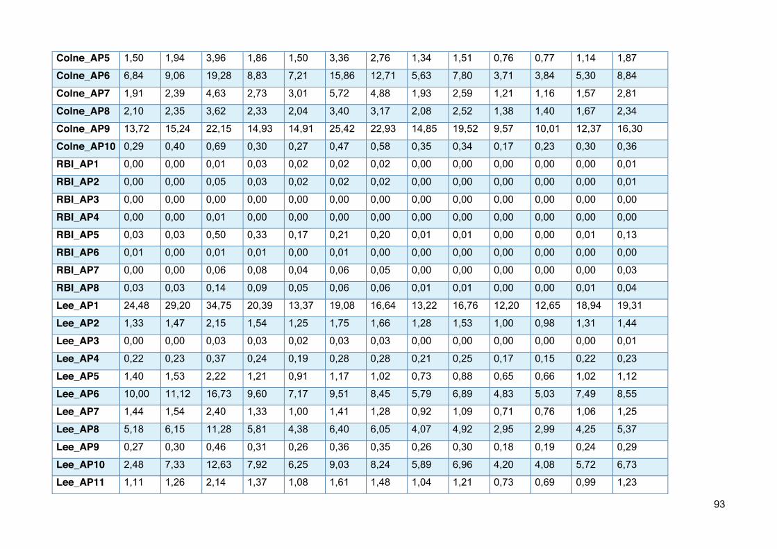
93

Colne_AP5 1,50 1,94 3,96 1,86 1,50 3,36 2,76 1,34 1,51 0,76 0,77 1,14 1,87

Colne_AP6 6,84 9,06 19,28 8,83 7,21 15,86 12,71 5,63 7,80 3,71 3,84 5,30 8,84

Colne_AP7 1,91 2,39 4,63 2,73 3,01 5,72 4,88 1,93 2,59 1,21 1,16 1,57 2,81

Colne_AP8 2,10 2,35 3,62 2,33 2,04 3,40 3,17 2,08 2,52 1,38 1,40 1,67 2,34

Colne_AP9 13,72 15,24 22,15 14,93 14,91 25,42 22,93 14,85 19,52 9,57 10,01 12,37 16,30

Colne_AP10 0,29 0,40 0,69 0,30 0,27 0,47 0,58 0,35 0,34 0,17 0,23 0,30 0,36

RBI_AP1 0,00 0,00 0,01 0,03 0,02 0,02 0,02 0,00 0,00 0,00 0,00 0,00 0,01

RBI_AP2 0,00 0,00 0,05 0,03 0,02 0,02 0,02 0,00 0,00 0,00 0,00 0,00 0,01

RBI_AP3 0,00 0,00 0,00 0,00 0,00 0,00 0,00 0,00 0,00 0,00 0,00 0,00 0,00

RBI_AP4 0,00 0,00 0,01 0,00 0,00 0,00 0,00 0,00 0,00 0,00 0,00 0,00 0,00

RBI_AP5 0,03 0,03 0,50 0,33 0,17 0,21 0,20 0,01 0,01 0,00 0,00 0,01 0,13

RBI_AP6 0,01 0,00 0,01 0,01 0,00 0,01 0,00 0,00 0,00 0,00 0,00 0,00 0,00

RBI_AP7 0,00 0,00 0,06 0,08 0,04 0,06 0,05 0,00 0,00 0,00 0,00 0,00 0,03

RBI_AP8 0,03 0,03 0,14 0,09 0,05 0,06 0,06 0,01 0,01 0,00 0,00 0,01 0,04

Lee_AP1 24,48 29,20 34,75 20,39 13,37 19,08 16,64 13,22 16,76 12,20 12,65 18,94 19,31

Lee_AP2 1,33 1,47 2,15 1,54 1,25 1,75 1,66 1,28 1,53 1,00 0,98 1,31 1,44

Lee_AP3 0,00 0,00 0,03 0,03 0,02 0,03 0,03 0,00 0,00 0,00 0,00 0,00 0,01

Lee_AP4 0,22 0,23 0,37 0,24 0,19 0,28 0,28 0,21 0,25 0,17 0,15 0,22 0,23

Lee_AP5 1,40 1,53 2,22 1,21 0,91 1,17 1,02 0,73 0,88 0,65 0,66 1,02 1,12

Lee_AP6 10,00 11,12 16,73 9,60 7,17 9,51 8,45 5,79 6,89 4,83 5,03 7,49 8,55

Lee_AP7 1,44 1,54 2,40 1,33 1,00 1,41 1,28 0,92 1,09 0,71 0,76 1,06 1,25

Lee_AP8 5,18 6,15 11,28 5,81 4,38 6,40 6,05 4,07 4,92 2,95 2,99 4,25 5,37

Lee_AP9 0,27 0,30 0,46 0,31 0,26 0,36 0,35 0,26 0,30 0,18 0,19 0,24 0,29

Lee_AP10 2,48 7,33 12,63 7,92 6,25 9,03 8,24 5,89 6,96 4,20 4,08 5,72 6,73

Lee_AP11 1,11 1,26 2,14 1,37 1,08 1,61 1,48 1,04 1,21 0,73 0,69 0,99 1,23

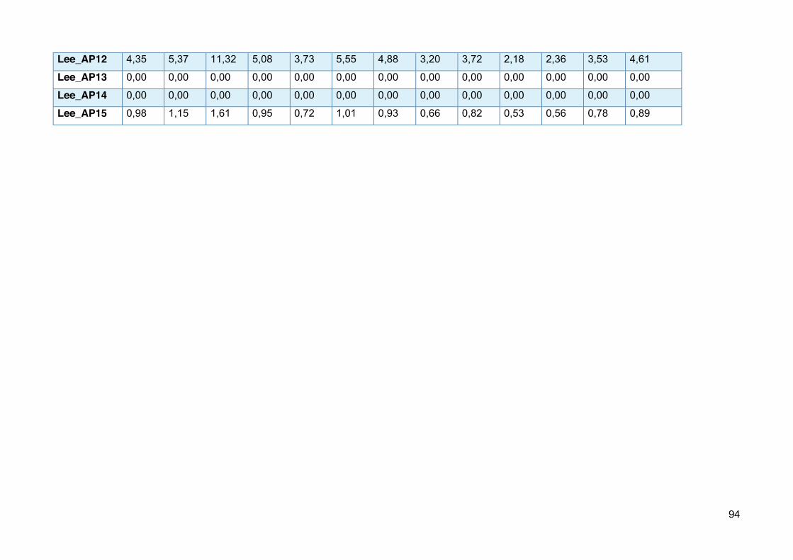
94

Lee_AP12 4,35 5,37 11,32 5,08 3,73 5,55 4,88 3,20 3,72 2,18 2,36 3,53 4,61

Lee_AP13 0,00 0,00 0,00 0,00 0,00 0,00 0,00 0,00 0,00 0,00 0,00 0,00 0,00

Lee_AP14 0,00 0,00 0,00 0,00 0,00 0,00 0,00 0,00 0,00 0,00 0,00 0,00 0,00

Lee_AP15 0,98 1,15 1,61 0,95 0,72 1,01 0,93 0,66 0,82 0,53 0,56 0,78 0,89

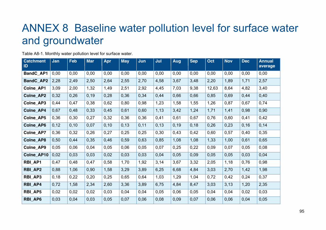
95

ANNEX 8 Baseline water pollution level for surface water and groundwater Table A8-1. Monthly water pollution level for surface water.

Catchment ID

Jan Feb Mar Apr May Jun Jul Aug Sep Oct Nov Dec Annual average

BandC_AP1 0,00 0,00 0,00 0,00 0,00 0,00 0,00 0,00 0,00 0,00 0,00 0,00 0,00

BandC_AP2 2,28 2,49 2,50 2,64 2,55 2,70 4,58 3,67 3,48 2,20 1,89 1,71 2,57

Colne_AP1 3,09 2,00 1,32 1,49 2,51 2,92 4,45 7,03 9,38 12,63 8,64 4,82 3,40

Colne_AP2 0,32 0,26 0,19 0,28 0,36 0,34 0,44 0,66 0,66 0,85 0,69 0,44 0,40

Colne_AP3 0,44 0,47 0,38 0,62 0,80 0,98 1,23 1,58 1,55 1,26 0,87 0,67 0,74

Colne_AP4 0,67 0,48 0,33 0,45 0,61 0,60 1,13 3,42 1,24 1,71 1,41 0,98 0,90

Colne_AP5 0,36 0,30 0,27 0,32 0,36 0,36 0,41 0,61 0,67 0,76 0,60 0,41 0,42

Colne_AP6 0,12 0,10 0,07 0,10 0,13 0,11 0,13 0,19 0,18 0,26 0,23 0,16 0,14

Colne_AP7 0,36 0,32 0,26 0,27 0,25 0,25 0,30 0,43 0,42 0,60 0,57 0,40 0,35

Colne_AP8 0,50 0,44 0,35 0,46 0,59 0,63 0,85 1,08 1,08 1,33 1,00 0,61 0,65

Colne_AP9 0,05 0,06 0,04 0,05 0,06 0,05 0,07 0,25 0,22 0,09 0,07 0,05 0,08

Colne_AP10 0,02 0,03 0,03 0,02 0,03 0,03 0,04 0,05 0,09 0,05 0,05 0,03 0,04

RBI_AP1 0,47 0,48 0,47 0,58 1,70 1,92 3,14 3,67 3,32 2,05 1,18 0,76 0,98

RBI_AP2 0,88 1,06 0,90 1,58 3,29 3,89 6,25 6,68 4,84 3,03 2,70 1,42 1,98

RBI_AP3 0,18 0,22 0,20 0,25 0,65 0,64 1,03 1,29 1,04 0,72 0,42 0,24 0,37

RBI_AP4 0,72 1,58 2,34 2,60 3,36 3,89 6,75 4,84 8,47 3,03 3,13 1,20 2,35

RBI_AP5 0,02 0,02 0,02 0,03 0,04 0,04 0,05 0,06 0,05 0,04 0,04 0,02 0,03

RBI_AP6 0,03 0,04 0,03 0,05 0,07 0,06 0,08 0,09 0,07 0,06 0,06 0,04 0,05

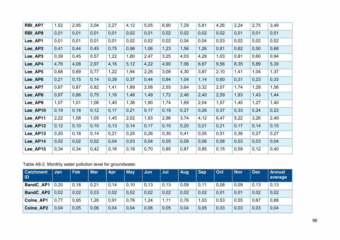
96

RBI_AP7 1,52 2,95 3,04 2,27 4,12 5,05 6,90 7,29 5,81 4,26 2,24 2,75 3,49

RBI_AP8 0,01 0,01 0,01 0,01 0,02 0,01 0,02 0,02 0,02 0,02 0,01 0,01 0,01

Lee_AP1 0,01 0,01 0,01 0,01 0,02 0,02 0,02 0,04 0,04 0,03 0,02 0,02 0,02

Lee_AP2 0,41 0,44 0,45 0,75 0,98 1,06 1,23 1,56 1,26 0,81 0,62 0,50 0,68

Lee_AP3 0,39 0,45 0,57 1,22 1,80 2,47 3,25 4,03 4,28 1,03 0,81 0,60 0,94

Lee_AP4 4,76 4,08 2,97 4,16 5,12 4,22 4,90 7,06 6,67 9,56 8,35 5,89 5,39

Lee_AP5 0,68 0,69 0,77 1,22 1,94 2,26 3,08 4,30 3,87 2,10 1,41 1,04 1,37

Lee_AP6 0,21 0,15 0,14 0,39 0,37 0,44 0,84 1,04 1,14 0,60 0,31 0,23 0,33

Lee_AP7 0,87 0,87 0,82 1,41 1,89 2,08 2,55 3,64 3,32 2,57 1,74 1,28 1,56

Lee_AP8 0,97 0,88 0,75 1,16 1,48 1,49 1,72 2,46 2,40 2,59 1,93 1,43 1,44

Lee_AP9 1,07 1,01 1,06 1,40 1,38 1,90 1,74 1,69 2,04 1,57 1,40 1,27 1,40

Lee_AP10 0,19 0,18 0,12 0,17 0,21 0,17 0,19 0,27 0,26 0,37 0,33 0,24 0,22

Lee_AP11 2,22 1,58 1,05 1,45 2,02 1,93 2,96 3,74 4,12 6,47 5,22 3,26 2,49

Lee_AP12 0,12 0,10 0,10 0,13 0,14 0,17 0,15 0,20 0,21 0,21 0,17 0,14 0,15

Lee_AP13 0,20 0,18 0,14 0,21 0,25 0,26 0,30 0,41 0,55 0,51 0,36 0,27 0,27

Lee_AP14 0,02 0,02 0,02 0,04 0,03 0,04 0,05 0,09 0,06 0,08 0,03 0,03 0,04

Lee_AP15 0,34 0,34 0,42 0,16 0,18 0,70 0,85 0,87 0,85 0,15 0,59 0,12 0,40

Table A8-2. Monthly water pollution level for groundwater.

Catchment ID

Jan Feb Mar Apr May Jun Jul Aug Sep Oct Nov Dec Annual average

BandC_AP1 0,20 0,18 0,21 0,14 0,10 0,13 0,13 0,09 0,11 0,08 0,09 0,13 0,13

BandC_AP2 0,02 0,02 0,03 0,02 0,02 0,02 0,02 0,02 0,02 0,01 0,01 0,02 0,02

Colne_AP1 0,77 0,95 1,26 0,91 0,76 1,24 1,11 0,76 1,03 0,53 0,55 0,67 0,88

Colne_AP2 0,04 0,05 0,06 0,04 0,04 0,06 0,05 0,04 0,05 0,03 0,03 0,03 0,04

97

Colne_AP3 0,02 0,03 0,05 0,02 0,02 0,03 0,03 0,02 0,02 0,01 0,01 0,02 0,02

Colne_AP4 0,11 0,15 0,24 0,14 0,11 0,21 0,17 0,10 0,15 0,07 0,07 0,09 0,13

Colne_AP5 0,12 0,18 0,34 0,17 0,13 0,28 0,22 0,11 0,15 0,07 0,07 0,09 0,16

Colne_AP6 0,01 0,01 0,02 0,01 0,01 0,02 0,02 0,01 0,01 0,00 0,01 0,01 0,01

Colne_AP7 0,05 0,07 0,12 0,07 0,05 0,10 0,08 0,05 0,07 0,03 0,03 0,04 0,06

Colne_AP8 0,38 0,47 0,65 0,43 0,36 0,61 0,54 0,36 0,49 0,25 0,26 0,33 0,43

Colne_AP9 0,96 1,20 1,63 1,08 0,92 1,53 1,36 0,92 1,25 0,64 0,66 0,82 1,08

Colne_AP10 4,98 6,21 8,45 5,59 4,74 7,94 7,02 4,75 6,48 3,30 3,42 4,28 5,60

RBI_AP1 0,00 0,00 0,00 0,00 0,00 0,00 0,00 0,00 0,00 0,00 0,00 0,00 0,00

RBI_AP2 0,23 0,20 0,22 0,15 0,07 0,09 0,08 0,06 0,08 0,05 0,06 0,09 0,11

RBI_AP3 1,03 0,93 1,02 0,67 0,33 0,41 0,38 0,26 0,34 0,23 0,27 0,41 0,52

RBI_AP4 0,00 0,00 0,00 0,00 0,00 0,00 0,00 0,00 0,00 0,00 0,00 0,00 0,00

RBI_AP5 0,00 0,00 0,00 0,00 0,00 0,00 0,00 0,00 0,00 0,00 0,00 0,00 0,00

RBI_AP6 0,00 0,00 0,00 0,00 0,00 0,00 0,00 0,00 0,00 0,00 0,00 0,00 0,00

RBI_AP7 0,04 0,04 0,04 0,03 0,01 0,02 0,01 0,01 0,01 0,01 0,01 0,02 0,02

RBI_AP8 0,00 0,00 0,00 0,00 0,00 0,00 0,00 0,00 0,00 0,00 0,00 0,00 0,00

Lee_AP1 0,07 0,08 0,10 0,06 0,04 0,06 0,05 0,04 0,05 0,03 0,04 0,05 0,06

Lee_AP2 0,02 0,03 0,04 0,03 0,02 0,03 0,03 0,02 0,03 0,02 0,02 0,02 0,02

Lee_AP3 0,23 0,14 0,11 0,06 0,05 0,06 0,06 0,04 0,05 0,04 0,05 0,07 0,08

Lee_AP4 0,03 0,04 0,05 0,04 0,03 0,04 0,04 0,03 0,04 0,02 0,02 0,03 0,03

Lee_AP5 0,11 0,13 0,17 0,10 0,07 0,10 0,09 0,06 0,08 0,05 0,06 0,08 0,09

Lee_AP6 0,15 0,18 0,25 0,14 0,10 0,14 0,13 0,09 0,11 0,08 0,08 0,12 0,13

Lee_AP7 0,06 0,07 0,10 0,06 0,04 0,06 0,05 0,04 0,05 0,03 0,03 0,05 0,05

Lee_AP8 0,10 0,13 0,22 0,12 0,08 0,13 0,11 0,08 0,10 0,06 0,06 0,08 0,11

Lee_AP9 0,46 0,56 0,77 0,53 0,42 0,59 0,56 0,42 0,51 0,32 0,32 0,42 0,49

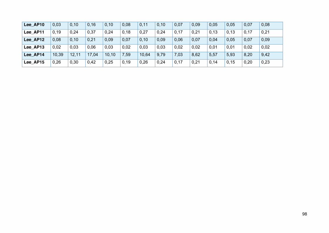
98

Lee_AP10 0,03 0,10 0,16 0,10 0,08 0,11 0,10 0,07 0,09 0,05 0,05 0,07 0,08

Lee_AP11 0,19 0,24 0,37 0,24 0,18 0,27 0,24 0,17 0,21 0,13 0,13 0,17 0,21

Lee_AP12 0,08 0,10 0,21 0,09 0,07 0,10 0,09 0,06 0,07 0,04 0,05 0,07 0,09

Lee_AP13 0,02 0,03 0,06 0,03 0,02 0,03 0,03 0,02 0,02 0,01 0,01 0,02 0,02

Lee_AP14 10,39 12,11 17,04 10,10 7,59 10,64 9,79 7,03 8,62 5,57 5,93 8,20 9,42

Lee_AP15 0,26 0,30 0,42 0,25 0,19 0,26 0,24 0,17 0,21 0,14 0,15 0,20 0,23

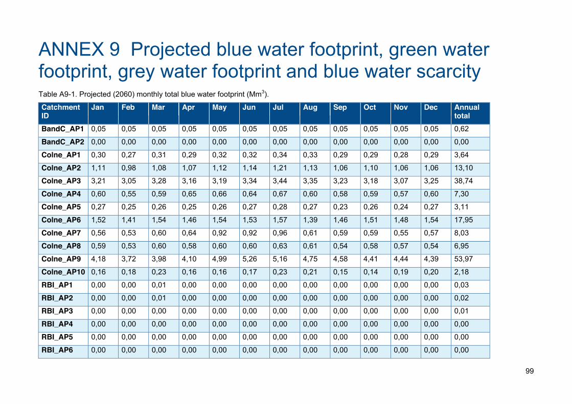
99

ANNEX 9 Projected blue water footprint, green water footprint, grey water footprint and blue water scarcity Table A9-1. Projected (2060) monthly total blue water footprint (Mm3).

Catchment ID

Jan Feb Mar Apr May Jun Jul Aug Sep Oct Nov Dec Annual total

BandC_AP1 0,05 0,05 0,05 0,05 0,05 0,05 0,05 0,05 0,05 0,05 0,05 0,05 0,62

BandC_AP2 0,00 0,00 0,00 0,00 0,00 0,00 0,00 0,00 0,00 0,00 0,00 0,00 0,00

Colne_AP1 0,30 0,27 0,31 0,29 0,32 0,32 0,34 0,33 0,29 0,29 0,28 0,29 3,64

Colne_AP2 1,11 0,98 1,08 1,07 1,12 1,14 1,21 1,13 1,06 1,10 1,06 1,06 13,10

Colne_AP3 3,21 3,05 3,28 3,16 3,19 3,34 3,44 3,35 3,23 3,18 3,07 3,25 38,74

Colne_AP4 0,60 0,55 0,59 0,65 0,66 0,64 0,67 0,60 0,58 0,59 0,57 0,60 7,30

Colne_AP5 0,27 0,25 0,26 0,25 0,26 0,27 0,28 0,27 0,23 0,26 0,24 0,27 3,11

Colne_AP6 1,52 1,41 1,54 1,46 1,54 1,53 1,57 1,39 1,46 1,51 1,48 1,54 17,95

Colne_AP7 0,56 0,53 0,60 0,64 0,92 0,92 0,96 0,61 0,59 0,59 0,55 0,57 8,03

Colne_AP8 0,59 0,53 0,60 0,58 0,60 0,60 0,63 0,61 0,54 0,58 0,57 0,54 6,95

Colne_AP9 4,18 3,72 3,98 4,10 4,99 5,26 5,16 4,75 4,58 4,41 4,44 4,39 53,97

Colne_AP10 0,16 0,18 0,23 0,16 0,16 0,17 0,23 0,21 0,15 0,14 0,19 0,20 2,18

RBI_AP1 0,00 0,00 0,01 0,00 0,00 0,00 0,00 0,00 0,00 0,00 0,00 0,00 0,03

RBI_AP2 0,00 0,00 0,01 0,00 0,00 0,00 0,00 0,00 0,00 0,00 0,00 0,00 0,02

RBI_AP3 0,00 0,00 0,00 0,00 0,00 0,00 0,00 0,00 0,00 0,00 0,00 0,00 0,01

RBI_AP4 0,00 0,00 0,00 0,00 0,00 0,00 0,00 0,00 0,00 0,00 0,00 0,00 0,00

RBI_AP5 0,00 0,00 0,00 0,00 0,00 0,00 0,00 0,00 0,00 0,00 0,00 0,00 0,00

RBI_AP6 0,00 0,00 0,00 0,00 0,00 0,00 0,00 0,00 0,00 0,00 0,00 0,00 0,00

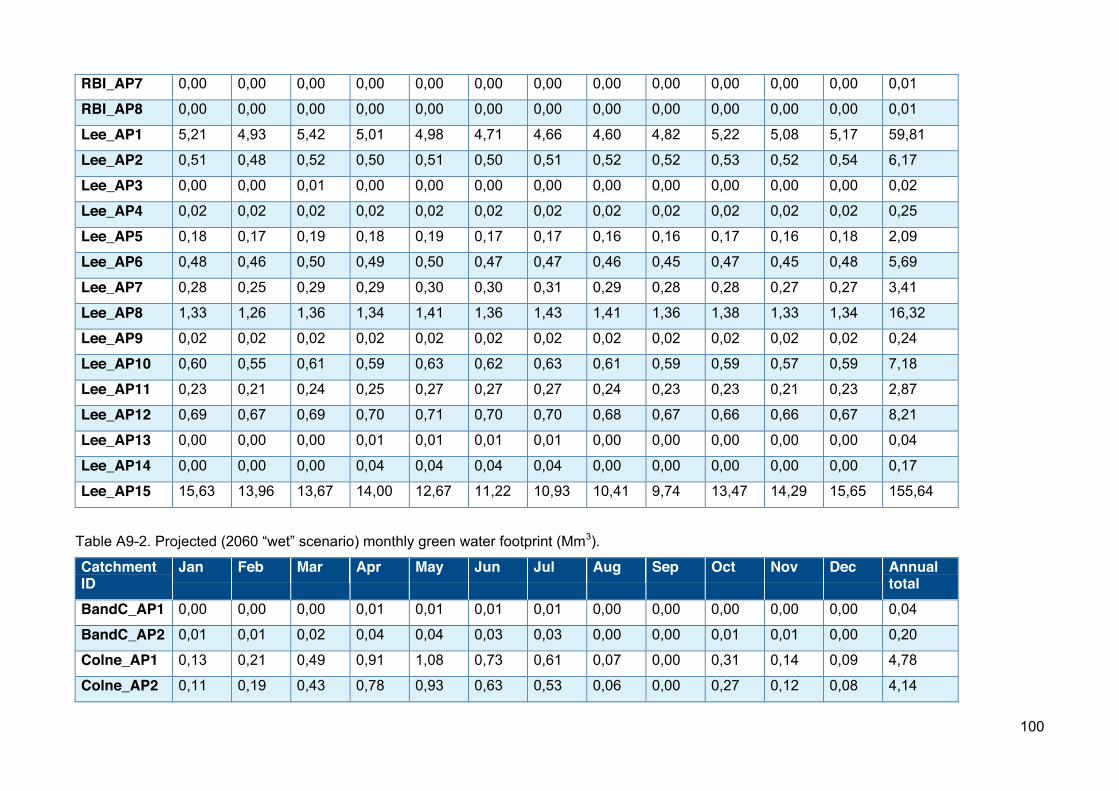
100

RBI_AP7 0,00 0,00 0,00 0,00 0,00 0,00 0,00 0,00 0,00 0,00 0,00 0,00 0,01

RBI_AP8 0,00 0,00 0,00 0,00 0,00 0,00 0,00 0,00 0,00 0,00 0,00 0,00 0,01

Lee_AP1 5,21 4,93 5,42 5,01 4,98 4,71 4,66 4,60 4,82 5,22 5,08 5,17 59,81

Lee_AP2 0,51 0,48 0,52 0,50 0,51 0,50 0,51 0,52 0,52 0,53 0,52 0,54 6,17

Lee_AP3 0,00 0,00 0,01 0,00 0,00 0,00 0,00 0,00 0,00 0,00 0,00 0,00 0,02

Lee_AP4 0,02 0,02 0,02 0,02 0,02 0,02 0,02 0,02 0,02 0,02 0,02 0,02 0,25

Lee_AP5 0,18 0,17 0,19 0,18 0,19 0,17 0,17 0,16 0,16 0,17 0,16 0,18 2,09

Lee_AP6 0,48 0,46 0,50 0,49 0,50 0,47 0,47 0,46 0,45 0,47 0,45 0,48 5,69

Lee_AP7 0,28 0,25 0,29 0,29 0,30 0,30 0,31 0,29 0,28 0,28 0,27 0,27 3,41

Lee_AP8 1,33 1,26 1,36 1,34 1,41 1,36 1,43 1,41 1,36 1,38 1,33 1,34 16,32

Lee_AP9 0,02 0,02 0,02 0,02 0,02 0,02 0,02 0,02 0,02 0,02 0,02 0,02 0,24

Lee_AP10 0,60 0,55 0,61 0,59 0,63 0,62 0,63 0,61 0,59 0,59 0,57 0,59 7,18

Lee_AP11 0,23 0,21 0,24 0,25 0,27 0,27 0,27 0,24 0,23 0,23 0,21 0,23 2,87

Lee_AP12 0,69 0,67 0,69 0,70 0,71 0,70 0,70 0,68 0,67 0,66 0,66 0,67 8,21

Lee_AP13 0,00 0,00 0,00 0,01 0,01 0,01 0,01 0,00 0,00 0,00 0,00 0,00 0,04

Lee_AP14 0,00 0,00 0,00 0,04 0,04 0,04 0,04 0,00 0,00 0,00 0,00 0,00 0,17

Lee_AP15 15,63 13,96 13,67 14,00 12,67 11,22 10,93 10,41 9,74 13,47 14,29 15,65 155,64

Table A9-2.  Projected  (2060  “wet”  scenario)  monthly  green  water  footprint  (Mm3).

Catchment ID

Jan Feb Mar Apr May Jun Jul Aug Sep Oct Nov Dec Annual total

BandC_AP1 0,00 0,00 0,00 0,01 0,01 0,01 0,01 0,00 0,00 0,00 0,00 0,00 0,04

BandC_AP2 0,01 0,01 0,02 0,04 0,04 0,03 0,03 0,00 0,00 0,01 0,01 0,00 0,20

Colne_AP1 0,13 0,21 0,49 0,91 1,08 0,73 0,61 0,07 0,00 0,31 0,14 0,09 4,78

Colne_AP2 0,11 0,19 0,43 0,78 0,93 0,63 0,53 0,06 0,00 0,27 0,12 0,08 4,14

101

Colne_AP3 0,38 0,64 1,48 2,71 3,23 2,19 1,84 0,22 0,00 0,94 0,42 0,28 14,34

Colne_AP4 0,08 0,14 0,32 0,59 0,69 0,47 0,40 0,05 0,00 0,21 0,09 0,06 3,10

Colne_AP5 0,10 0,17 0,40 0,73 0,86 0,59 0,49 0,06 0,00 0,26 0,11 0,07 3,86

Colne_AP6 0,12 0,20 0,46 0,84 1,00 0,68 0,57 0,07 0,00 0,29 0,13 0,09 4,44

Colne_AP7 0,09 0,15 0,35 0,65 0,79 0,54 0,46 0,06 0,00 0,22 0,10 0,06 3,48

Colne_AP8 0,07 0,12 0,29 0,53 0,66 0,45 0,38 0,05 0,00 0,18 0,08 0,05 2,86

Colne_AP9 0,12 0,20 0,46 0,84 1,02 0,70 0,58 0,07 0,00 0,29 0,13 0,08 4,48

Colne_AP10 0,14 0,24 0,55 1,04 1,27 0,88 0,73 0,09 0,00 0,35 0,15 0,10 5,54

Lee_AP1 0,07 0,11 0,25 0,48 0,55 0,37 0,39 0,05 0,00 0,20 0,09 0,06 2,61

Lee_AP2 0,57 0,94 2,16 3,89 4,51 3,01 2,55 0,30 0,00 1,38 0,62 0,41 20,34

Lee_AP3 0,17 0,27 0,63 1,13 1,31 0,87 0,74 0,09 0,00 0,40 0,18 0,12 5,91

Lee_AP4 0,15 0,25 0,57 1,04 1,20 0,80 0,68 0,08 0,00 0,37 0,16 0,11 5,41

Lee_AP5 0,28 0,47 1,10 1,96 2,25 1,50 1,22 0,14 0,00 0,68 0,30 0,20 10,09

Lee_AP6 0,11 0,18 0,40 0,74 0,86 0,58 0,51 0,06 0,00 0,27 0,12 0,08 3,90

Lee_AP7 0,43 0,71 1,61 2,94 3,42 2,31 2,04 0,24 0,00 1,09 0,49 0,32 15,59

Lee_AP8 0,43 0,72 1,68 3,05 3,56 2,40 2,01 0,24 0,00 1,08 0,48 0,31 15,99

Lee_AP9 0,11 0,19 0,44 0,79 0,93 0,63 0,52 0,06 0,00 0,28 0,13 0,08 4,16

Lee_AP10 0,11 0,20 0,46 0,84 0,99 0,67 0,56 0,07 0,00 0,29 0,13 0,08 4,42

Lee_AP11 0,25 0,43 1,00 1,83 2,16 1,47 1,23 0,15 0,00 0,64 0,29 0,18 9,61

Lee_AP12 0,10 0,15 0,34 0,65 0,76 0,51 0,53 0,06 0,00 0,27 0,12 0,08 3,56

Lee_AP13 0,08 0,13 0,28 0,54 0,63 0,43 0,45 0,05 0,00 0,23 0,10 0,06 2,99

Lee_AP14 0,15 0,24 0,54 1,02 1,19 0,80 0,84 0,10 0,00 0,43 0,19 0,12 5,62

Lee_AP15 0,02 0,03 0,06 0,11 0,13 0,09 0,09 0,01 0,00 0,05 0,02 0,01 0,62

RBI_AP1 0,24 0,40 0,96 1,68 1,92 1,23 0,93 0,11 0,00 0,52 0,23 0,16 8,37

RBI_AP2 0,46 0,76 1,76 3,18 3,66 2,44 2,07 0,28 0,03 1,12 0,50 0,33 16,58

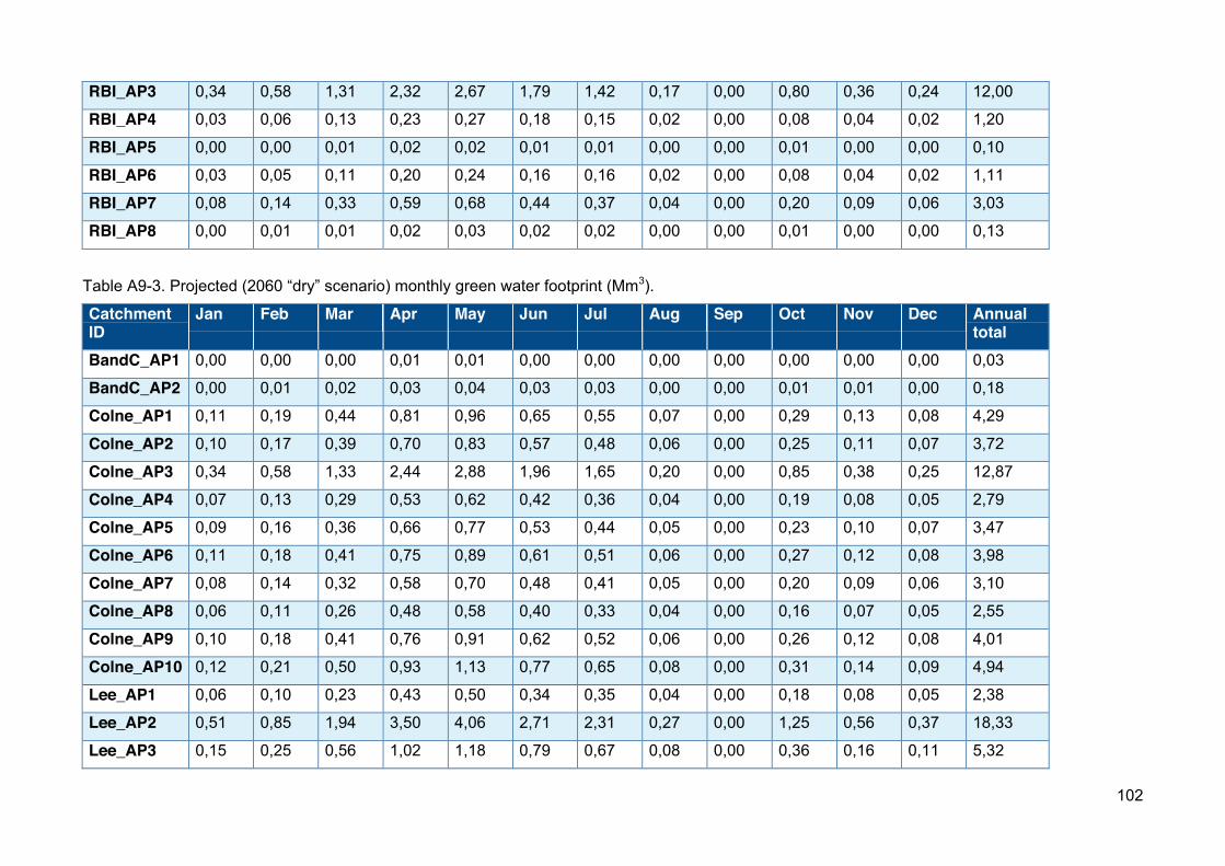
102

RBI_AP3 0,34 0,58 1,31 2,32 2,67 1,79 1,42 0,17 0,00 0,80 0,36 0,24 12,00

RBI_AP4 0,03 0,06 0,13 0,23 0,27 0,18 0,15 0,02 0,00 0,08 0,04 0,02 1,20

RBI_AP5 0,00 0,00 0,01 0,02 0,02 0,01 0,01 0,00 0,00 0,01 0,00 0,00 0,10

RBI_AP6 0,03 0,05 0,11 0,20 0,24 0,16 0,16 0,02 0,00 0,08 0,04 0,02 1,11

RBI_AP7 0,08 0,14 0,33 0,59 0,68 0,44 0,37 0,04 0,00 0,20 0,09 0,06 3,03

RBI_AP8 0,00 0,01 0,01 0,02 0,03 0,02 0,02 0,00 0,00 0,01 0,00 0,00 0,13

Table A9-3.  Projected  (2060  “dry”  scenario)  monthly  green  water  footprint  (Mm3).

Catchment ID

Jan Feb Mar Apr May Jun Jul Aug Sep Oct Nov Dec Annual total

BandC_AP1 0,00 0,00 0,00 0,01 0,01 0,00 0,00 0,00 0,00 0,00 0,00 0,00 0,03

BandC_AP2 0,00 0,01 0,02 0,03 0,04 0,03 0,03 0,00 0,00 0,01 0,01 0,00 0,18

Colne_AP1 0,11 0,19 0,44 0,81 0,96 0,65 0,55 0,07 0,00 0,29 0,13 0,08 4,29

Colne_AP2 0,10 0,17 0,39 0,70 0,83 0,57 0,48 0,06 0,00 0,25 0,11 0,07 3,72

Colne_AP3 0,34 0,58 1,33 2,44 2,88 1,96 1,65 0,20 0,00 0,85 0,38 0,25 12,87

Colne_AP4 0,07 0,13 0,29 0,53 0,62 0,42 0,36 0,04 0,00 0,19 0,08 0,05 2,79

Colne_AP5 0,09 0,16 0,36 0,66 0,77 0,53 0,44 0,05 0,00 0,23 0,10 0,07 3,47

Colne_AP6 0,11 0,18 0,41 0,75 0,89 0,61 0,51 0,06 0,00 0,27 0,12 0,08 3,98

Colne_AP7 0,08 0,14 0,32 0,58 0,70 0,48 0,41 0,05 0,00 0,20 0,09 0,06 3,10

Colne_AP8 0,06 0,11 0,26 0,48 0,58 0,40 0,33 0,04 0,00 0,16 0,07 0,05 2,55

Colne_AP9 0,10 0,18 0,41 0,76 0,91 0,62 0,52 0,06 0,00 0,26 0,12 0,08 4,01

Colne_AP10 0,12 0,21 0,50 0,93 1,13 0,77 0,65 0,08 0,00 0,31 0,14 0,09 4,94

Lee_AP1 0,06 0,10 0,23 0,43 0,50 0,34 0,35 0,04 0,00 0,18 0,08 0,05 2,38

Lee_AP2 0,51 0,85 1,94 3,50 4,06 2,71 2,31 0,27 0,00 1,25 0,56 0,37 18,33

Lee_AP3 0,15 0,25 0,56 1,02 1,18 0,79 0,67 0,08 0,00 0,36 0,16 0,11 5,32

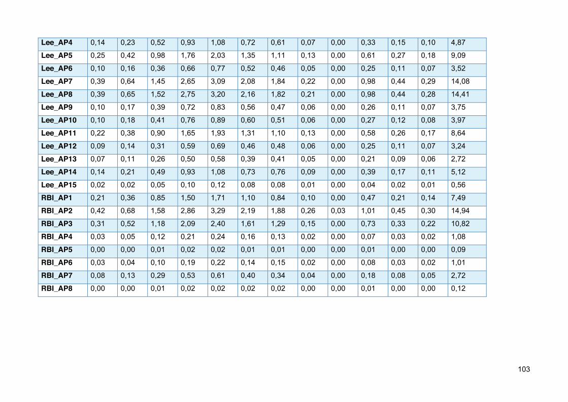
103

Lee_AP4 0,14 0,23 0,52 0,93 1,08 0,72 0,61 0,07 0,00 0,33 0,15 0,10 4,87

Lee_AP5 0,25 0,42 0,98 1,76 2,03 1,35 1,11 0,13 0,00 0,61 0,27 0,18 9,09

Lee_AP6 0,10 0,16 0,36 0,66 0,77 0,52 0,46 0,05 0,00 0,25 0,11 0,07 3,52

Lee_AP7 0,39 0,64 1,45 2,65 3,09 2,08 1,84 0,22 0,00 0,98 0,44 0,29 14,08

Lee_AP8 0,39 0,65 1,52 2,75 3,20 2,16 1,82 0,21 0,00 0,98 0,44 0,28 14,41

Lee_AP9 0,10 0,17 0,39 0,72 0,83 0,56 0,47 0,06 0,00 0,26 0,11 0,07 3,75

Lee_AP10 0,10 0,18 0,41 0,76 0,89 0,60 0,51 0,06 0,00 0,27 0,12 0,08 3,97

Lee_AP11 0,22 0,38 0,90 1,65 1,93 1,31 1,10 0,13 0,00 0,58 0,26 0,17 8,64

Lee_AP12 0,09 0,14 0,31 0,59 0,69 0,46 0,48 0,06 0,00 0,25 0,11 0,07 3,24

Lee_AP13 0,07 0,11 0,26 0,50 0,58 0,39 0,41 0,05 0,00 0,21 0,09 0,06 2,72

Lee_AP14 0,14 0,21 0,49 0,93 1,08 0,73 0,76 0,09 0,00 0,39 0,17 0,11 5,12

Lee_AP15 0,02 0,02 0,05 0,10 0,12 0,08 0,08 0,01 0,00 0,04 0,02 0,01 0,56

RBI_AP1 0,21 0,36 0,85 1,50 1,71 1,10 0,84 0,10 0,00 0,47 0,21 0,14 7,49

RBI_AP2 0,42 0,68 1,58 2,86 3,29 2,19 1,88 0,26 0,03 1,01 0,45 0,30 14,94

RBI_AP3 0,31 0,52 1,18 2,09 2,40 1,61 1,29 0,15 0,00 0,73 0,33 0,22 10,82

RBI_AP4 0,03 0,05 0,12 0,21 0,24 0,16 0,13 0,02 0,00 0,07 0,03 0,02 1,08

RBI_AP5 0,00 0,00 0,01 0,02 0,02 0,01 0,01 0,00 0,00 0,01 0,00 0,00 0,09

RBI_AP6 0,03 0,04 0,10 0,19 0,22 0,14 0,15 0,02 0,00 0,08 0,03 0,02 1,01

RBI_AP7 0,08 0,13 0,29 0,53 0,61 0,40 0,34 0,04 0,00 0,18 0,08 0,05 2,72

RBI_AP8 0,00 0,00 0,01 0,02 0,02 0,02 0,02 0,00 0,00 0,01 0,00 0,00 0,12

104

Table A9-4. Projected (2060) monthly total grey water footprint (Mm3).

Catchment ID

Jan Feb Mar Apr May Jun Jul Aug Sep Oct Nov Dec Annual Total

BandC_AP1 0,27 0,27 0,27 0,28 0,27 0,27 0,27 0,27 0,27 0,28 0,27 0,27 3,26

BandC_AP2 11,48 11,34 11,58 10,87 10,47 9,05 10,97 10,04 7,27 7,94 7,85 7,75 116,61

Colne_AP1 2,26 2,13 1,96 2,12 2,29 2,04 2,09 2,28 2,13 2,54 2,53 2,32 26,71

Colne_AP2 0,66 0,58 0,46 0,58 0,69 0,52 0,55 0,69 0,58 0,87 0,86 0,71 7,74

Colne_AP3 2,54 2,45 1,92 2,34 2,66 2,22 2,22 2,58 2,15 3,06 3,05 2,92 30,10

Colne_AP4 0,52 0,45 0,38 0,43 0,51 0,42 0,61 1,46 0,47 0,61 0,60 0,57 7,04

Colne_AP5 0,79 0,71 0,72 0,76 0,80 0,72 0,74 0,85 0,68 0,83 0,83 0,73 9,17

Colne_AP6 0,48 0,42 0,33 0,42 0,51 0,37 0,40 0,51 0,42 0,65 0,64 0,52 5,69

Colne_AP7 0,84 0,80 0,79 0,77 0,65 0,56 0,59 0,70 0,59 0,80 0,82 0,72 8,62

Colne_AP8 1,29 1,25 1,20 1,22 1,27 1,18 1,20 1,24 1,17 1,36 1,38 1,28 15,04

Colne_AP9 3,35 3,37 3,06 3,19 3,34 3,01 3,13 4,97 4,30 3,26 3,26 3,17 41,41

Colne_AP10 23,08 23,13 23,17 23,02 23,12 22,97 23,00 23,12 23,42 23,24 23,41 23,20 277,86

RBI_AP1 1,24 1,09 0,87 1,07 1,36 0,96 1,01 1,29 1,07 1,65 1,63 1,37 14,62

RBI_AP2 2,75 2,54 1,97 2,40 2,94 2,13 2,32 2,87 2,39 3,74 4,55 3,06 33,65

RBI_AP3 2,10 2,06 1,76 1,85 2,24 1,70 1,79 2,12 1,81 2,51 2,58 2,23 24,73

RBI_AP4 9,11 15,14 19,57 16,59 12,40 9,90 11,73 8,52 14,64 12,41 19,55 12,35 161,91

RBI_AP5 0,00 0,00 0,00 0,00 0,00 0,00 0,00 0,00 0,00 0,01 0,01 0,00 0,05

RBI_AP6 0,05 0,04 0,03 0,04 0,05 0,04 0,04 0,05 0,04 0,07 0,07 0,05 0,60

RBI_AP7 3,01 4,69 4,39 2,70 4,03 3,95 4,89 5,35 4,44 4,95 2,96 4,43 49,79

RBI_AP8 0,00 0,00 0,00 0,00 0,00 0,00 0,00 0,00 0,00 0,00 0,00 0,00 0,03

Lee_AP1 0,22 0,20 0,16 0,20 0,23 0,18 0,19 0,23 0,19 0,28 0,28 0,23 2,58

Lee_AP2 3,78 3,25 2,71 2,99 3,69 2,60 2,77 3,46 2,87 4,16 4,15 3,51 39,92

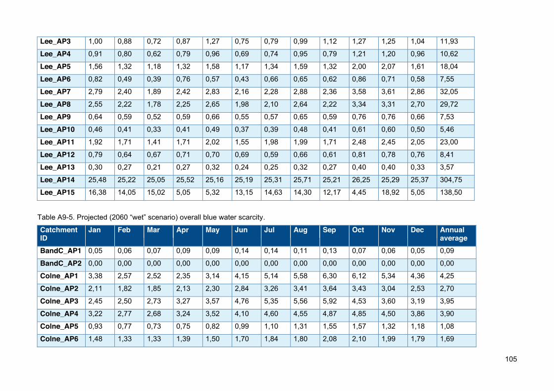
105

Lee_AP3 1,00 0,88 0,72 0,87 1,27 0,75 0,79 0,99 1,12 1,27 1,25 1,04 11,93

Lee_AP4 0,91 0,80 0,62 0,79 0,96 0,69 0,74 0,95 0,79 1,21 1,20 0,96 10,62

Lee_AP5 1,56 1,32 1,18 1,32 1,58 1,17 1,34 1,59 1,32 2,00 2,07 1,61 18,04

Lee_AP6 0,82 0,49 0,39 0,76 0,57 0,43 0,66 0,65 0,62 0,86 0,71 0,58 7,55

Lee_AP7 2,79 2,40 1,89 2,42 2,83 2,16 2,28 2,88 2,36 3,58 3,61 2,86 32,05

Lee_AP8 2,55 2,22 1,78 2,25 2,65 1,98 2,10 2,64 2,22 3,34 3,31 2,70 29,72

Lee_AP9 0,64 0,59 0,52 0,59 0,66 0,55 0,57 0,65 0,59 0,76 0,76 0,66 7,53

Lee_AP10 0,46 0,41 0,33 0,41 0,49 0,37 0,39 0,48 0,41 0,61 0,60 0,50 5,46

Lee_AP11 1,92 1,71 1,41 1,71 2,02 1,55 1,98 1,99 1,71 2,48 2,45 2,05 23,00

Lee_AP12 0,79 0,64 0,67 0,71 0,70 0,69 0,59 0,66 0,61 0,81 0,78 0,76 8,41

Lee_AP13 0,30 0,27 0,21 0,27 0,32 0,24 0,25 0,32 0,27 0,40 0,40 0,33 3,57

Lee_AP14 25,48 25,22 25,05 25,52 25,16 25,19 25,31 25,71 25,21 26,25 25,29 25,37 304,75

Lee_AP15 16,38 14,05 15,02 5,05 5,32 13,15 14,63 14,30 12,17 4,45 18,92 5,05 138,50

Table A9-5.  Projected  (2060  “wet”  scenario)  overall  blue  water  scarcity.

Catchment ID

Jan Feb Mar Apr May Jun Jul Aug Sep Oct Nov Dec Annual average

BandC_AP1 0,05 0,06 0,07 0,09 0,09 0,14 0,14 0,11 0,13 0,07 0,06 0,05 0,09

BandC_AP2 0,00 0,00 0,00 0,00 0,00 0,00 0,00 0,00 0,00 0,00 0,00 0,00 0,00

Colne_AP1 3,38 2,57 2,52 2,35 3,14 4,15 5,14 5,58 6,30 6,12 5,34 4,36 4,25

Colne_AP2 2,11 1,82 1,85 2,13 2,30 2,84 3,26 3,41 3,64 3,43 3,04 2,53 2,70

Colne_AP3 2,45 2,50 2,73 3,27 3,57 4,76 5,35 5,56 5,92 4,53 3,60 3,19 3,95

Colne_AP4 3,22 2,77 2,68 3,24 3,52 4,10 4,60 4,55 4,87 4,85 4,50 3,86 3,90

Colne_AP5 0,93 0,77 0,73 0,75 0,82 0,99 1,10 1,31 1,55 1,57 1,32 1,18 1,08

Colne_AP6 1,48 1,33 1,33 1,39 1,50 1,70 1,84 1,80 2,08 2,10 1,99 1,79 1,69

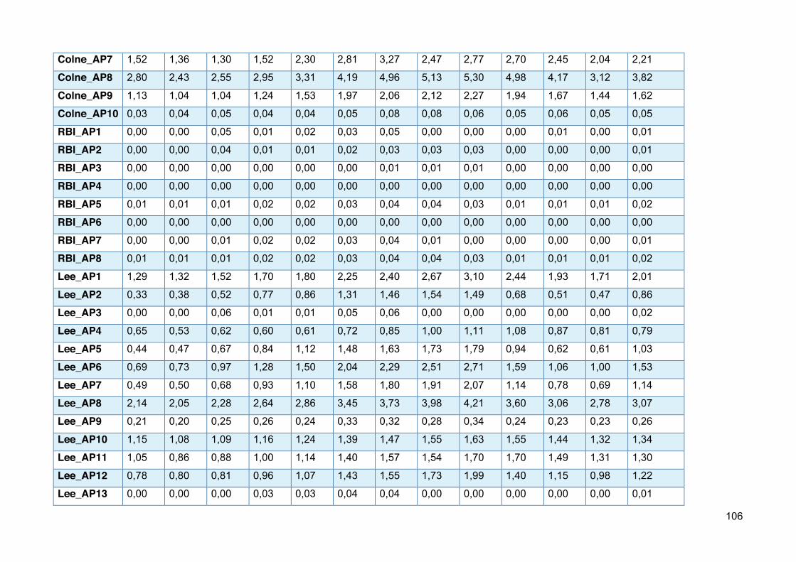
106

Colne_AP7 1,52 1,36 1,30 1,52 2,30 2,81 3,27 2,47 2,77 2,70 2,45 2,04 2,21

Colne_AP8 2,80 2,43 2,55 2,95 3,31 4,19 4,96 5,13 5,30 4,98 4,17 3,12 3,82

Colne_AP9 1,13 1,04 1,04 1,24 1,53 1,97 2,06 2,12 2,27 1,94 1,67 1,44 1,62

Colne_AP10 0,03 0,04 0,05 0,04 0,04 0,05 0,08 0,08 0,06 0,05 0,06 0,05 0,05

RBI_AP1 0,00 0,00 0,05 0,01 0,02 0,03 0,05 0,00 0,00 0,00 0,01 0,00 0,01

RBI_AP2 0,00 0,00 0,04 0,01 0,01 0,02 0,03 0,03 0,03 0,00 0,00 0,00 0,01

RBI_AP3 0,00 0,00 0,00 0,00 0,00 0,00 0,01 0,01 0,01 0,00 0,00 0,00 0,00

RBI_AP4 0,00 0,00 0,00 0,00 0,00 0,00 0,00 0,00 0,00 0,00 0,00 0,00 0,00

RBI_AP5 0,01 0,01 0,01 0,02 0,02 0,03 0,04 0,04 0,03 0,01 0,01 0,01 0,02

RBI_AP6 0,00 0,00 0,00 0,00 0,00 0,00 0,00 0,00 0,00 0,00 0,00 0,00 0,00

RBI_AP7 0,00 0,00 0,01 0,02 0,02 0,03 0,04 0,01 0,00 0,00 0,00 0,00 0,01

RBI_AP8 0,01 0,01 0,01 0,02 0,02 0,03 0,04 0,04 0,03 0,01 0,01 0,01 0,02

Lee_AP1 1,29 1,32 1,52 1,70 1,80 2,25 2,40 2,67 3,10 2,44 1,93 1,71 2,01

Lee_AP2 0,33 0,38 0,52 0,77 0,86 1,31 1,46 1,54 1,49 0,68 0,51 0,47 0,86

Lee_AP3 0,00 0,00 0,06 0,01 0,01 0,05 0,06 0,00 0,00 0,00 0,00 0,00 0,02

Lee_AP4 0,65 0,53 0,62 0,60 0,61 0,72 0,85 1,00 1,11 1,08 0,87 0,81 0,79

Lee_AP5 0,44 0,47 0,67 0,84 1,12 1,48 1,63 1,73 1,79 0,94 0,62 0,61 1,03

Lee_AP6 0,69 0,73 0,97 1,28 1,50 2,04 2,29 2,51 2,71 1,59 1,06 1,00 1,53

Lee_AP7 0,49 0,50 0,68 0,93 1,10 1,58 1,80 1,91 2,07 1,14 0,78 0,69 1,14

Lee_AP8 2,14 2,05 2,28 2,64 2,86 3,45 3,73 3,98 4,21 3,60 3,06 2,78 3,07

Lee_AP9 0,21 0,20 0,25 0,26 0,24 0,33 0,32 0,28 0,34 0,24 0,23 0,23 0,26

Lee_AP10 1,15 1,08 1,09 1,16 1,24 1,39 1,47 1,55 1,63 1,55 1,44 1,32 1,34

Lee_AP11 1,05 0,86 0,88 1,00 1,14 1,40 1,57 1,54 1,70 1,70 1,49 1,31 1,30

Lee_AP12 0,78 0,80 0,81 0,96 1,07 1,43 1,55 1,73 1,99 1,40 1,15 0,98 1,22

Lee_AP13 0,00 0,00 0,00 0,03 0,03 0,04 0,04 0,00 0,00 0,00 0,00 0,00 0,01

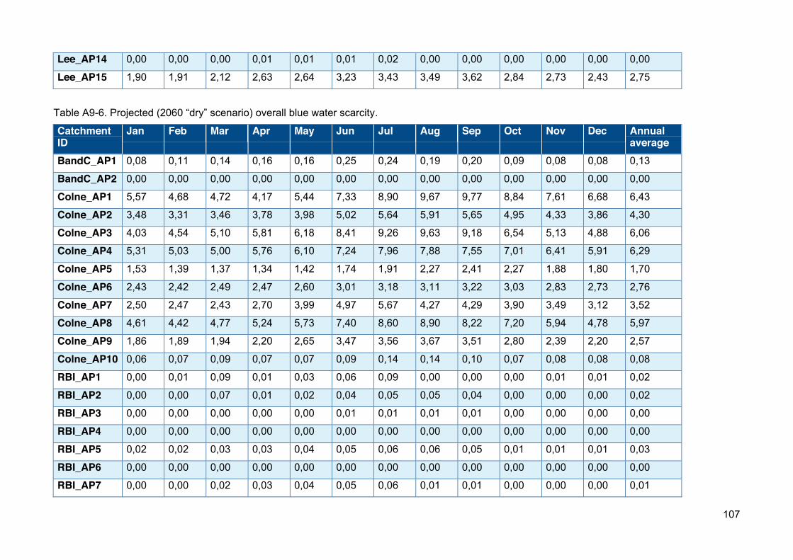
107

Lee_AP14 0,00 0,00 0,00 0,01 0,01 0,01 0,02 0,00 0,00 0,00 0,00 0,00 0,00

Lee_AP15 1,90 1,91 2,12 2,63 2,64 3,23 3,43 3,49 3,62 2,84 2,73 2,43 2,75

Table A9-6.  Projected  (2060  “dry”  scenario)  overall  blue  water  scarcity.

Catchment ID

Jan Feb Mar Apr May Jun Jul Aug Sep Oct Nov Dec Annual average

BandC_AP1 0,08 0,11 0,14 0,16 0,16 0,25 0,24 0,19 0,20 0,09 0,08 0,08 0,13

BandC_AP2 0,00 0,00 0,00 0,00 0,00 0,00 0,00 0,00 0,00 0,00 0,00 0,00 0,00

Colne_AP1 5,57 4,68 4,72 4,17 5,44 7,33 8,90 9,67 9,77 8,84 7,61 6,68 6,43

Colne_AP2 3,48 3,31 3,46 3,78 3,98 5,02 5,64 5,91 5,65 4,95 4,33 3,86 4,30

Colne_AP3 4,03 4,54 5,10 5,81 6,18 8,41 9,26 9,63 9,18 6,54 5,13 4,88 6,06

Colne_AP4 5,31 5,03 5,00 5,76 6,10 7,24 7,96 7,88 7,55 7,01 6,41 5,91 6,29

Colne_AP5 1,53 1,39 1,37 1,34 1,42 1,74 1,91 2,27 2,41 2,27 1,88 1,80 1,70

Colne_AP6 2,43 2,42 2,49 2,47 2,60 3,01 3,18 3,11 3,22 3,03 2,83 2,73 2,76

Colne_AP7 2,50 2,47 2,43 2,70 3,99 4,97 5,67 4,27 4,29 3,90 3,49 3,12 3,52

Colne_AP8 4,61 4,42 4,77 5,24 5,73 7,40 8,60 8,90 8,22 7,20 5,94 4,78 5,97

Colne_AP9 1,86 1,89 1,94 2,20 2,65 3,47 3,56 3,67 3,51 2,80 2,39 2,20 2,57

Colne_AP10 0,06 0,07 0,09 0,07 0,07 0,09 0,14 0,14 0,10 0,07 0,08 0,08 0,08

RBI_AP1 0,00 0,01 0,09 0,01 0,03 0,06 0,09 0,00 0,00 0,00 0,01 0,01 0,02

RBI_AP2 0,00 0,00 0,07 0,01 0,02 0,04 0,05 0,05 0,04 0,00 0,00 0,00 0,02

RBI_AP3 0,00 0,00 0,00 0,00 0,00 0,01 0,01 0,01 0,01 0,00 0,00 0,00 0,00

RBI_AP4 0,00 0,00 0,00 0,00 0,00 0,00 0,00 0,00 0,00 0,00 0,00 0,00 0,00

RBI_AP5 0,02 0,02 0,03 0,03 0,04 0,05 0,06 0,06 0,05 0,01 0,01 0,01 0,03

RBI_AP6 0,00 0,00 0,00 0,00 0,00 0,00 0,00 0,00 0,00 0,00 0,00 0,00 0,00

RBI_AP7 0,00 0,00 0,02 0,03 0,04 0,05 0,06 0,01 0,01 0,00 0,00 0,00 0,01

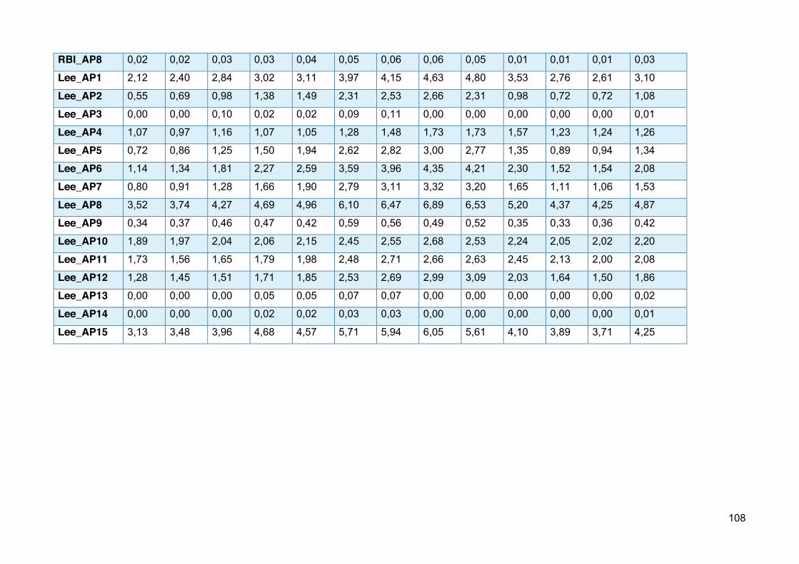
108

RBI_AP8 0,02 0,02 0,03 0,03 0,04 0,05 0,06 0,06 0,05 0,01 0,01 0,01 0,03

Lee_AP1 2,12 2,40 2,84 3,02 3,11 3,97 4,15 4,63 4,80 3,53 2,76 2,61 3,10

Lee_AP2 0,55 0,69 0,98 1,38 1,49 2,31 2,53 2,66 2,31 0,98 0,72 0,72 1,08

Lee_AP3 0,00 0,00 0,10 0,02 0,02 0,09 0,11 0,00 0,00 0,00 0,00 0,00 0,01

Lee_AP4 1,07 0,97 1,16 1,07 1,05 1,28 1,48 1,73 1,73 1,57 1,23 1,24 1,26

Lee_AP5 0,72 0,86 1,25 1,50 1,94 2,62 2,82 3,00 2,77 1,35 0,89 0,94 1,34

Lee_AP6 1,14 1,34 1,81 2,27 2,59 3,59 3,96 4,35 4,21 2,30 1,52 1,54 2,08

Lee_AP7 0,80 0,91 1,28 1,66 1,90 2,79 3,11 3,32 3,20 1,65 1,11 1,06 1,53

Lee_AP8 3,52 3,74 4,27 4,69 4,96 6,10 6,47 6,89 6,53 5,20 4,37 4,25 4,87

Lee_AP9 0,34 0,37 0,46 0,47 0,42 0,59 0,56 0,49 0,52 0,35 0,33 0,36 0,42

Lee_AP10 1,89 1,97 2,04 2,06 2,15 2,45 2,55 2,68 2,53 2,24 2,05 2,02 2,20

Lee_AP11 1,73 1,56 1,65 1,79 1,98 2,48 2,71 2,66 2,63 2,45 2,13 2,00 2,08

Lee_AP12 1,28 1,45 1,51 1,71 1,85 2,53 2,69 2,99 3,09 2,03 1,64 1,50 1,86

Lee_AP13 0,00 0,00 0,00 0,05 0,05 0,07 0,07 0,00 0,00 0,00 0,00 0,00 0,02

Lee_AP14 0,00 0,00 0,00 0,02 0,02 0,03 0,03 0,00 0,00 0,00 0,00 0,00 0,01

Lee_AP15 3,13 3,48 3,96 4,68 4,57 5,71 5,94 6,05 5,61 4,10 3,89 3,71 4,25

109

Acknowledgements This report is an outcome of partnership project carried out by the Water Footprint Network and the Environment Agency, Hertfordshire and North London, UK. The Environment Agency funded this study. The University of Twente provided technical support to this study.

110

List of abbreviations AP Assessment Point

ASB Abstraction Sensitivity Band

BAT Best Available Technology

BP Best Practices

BWS Blue Water Scarcity

CAMS Catchment Abstraction Management Strategies

Defra Department for Environment, Food & Rural Affairs (UK)

EA Environment Agency (UK)

EFI Environmental Flow Indicator

EFR Environmental Flow Requirements

IWRM Integrated Water Resources Management

Mm3 Million cubic meters

RBI Roding-Beam-Ingrebourne

RSA Restoring Sustainable Abstraction

SENET South East Region North East Thames Area

STW Sewage Treatment Works

WF Water footprint

WFA Water Footprint Assessment

WFD Water Framework Directive

WFN Water Footprint Network

WPL Water Pollution Level

111

www.gov.uk/environment-agency