wine analytics: fine wine pricing and selection under
TRANSCRIPT
MANUFACTURING & SERVICE OPERATIONS MANAGEMENTVol. 19, No. 2, Spring 2017, pp. 202–215
http://pubsonline.informs.org/journal/msom/ ISSN 1523-4614 (print), ISSN 1526-5498 (online)
Wine Analytics: Fine Wine Pricing and Selection Under Weatherand Market UncertaintyMert Hakan Hekimoğlu,a Burak Kazaz,b Scott WebstercaLally School of Management, Rensselaer Polytechnic Institute, Troy, New York 12180; bWhitman School of Management, SyracuseUniversity, Syracuse, New York 13244; cW. P. Carey School of Business, Arizona State University, Tempe, Arizona 85287Contact: [email protected] (MHH); [email protected] (BK); [email protected] (SW)
Received: July 22, 2015Revised: November 12, 2015; March 24, 2016;July 23, 2016Accepted: September 5, 2016Published Online in Articles in Advance:November 29, 2016
https://doi.org/10.1287/msom.2016.0602
Copyright: © 2016 INFORMS
Abstract. We examine a risk-averse distributor’s decision in selecting between bottledwine and wine futures under weather and market uncertainty. At the beginning of everysummer, a fine wine distributor has to choose between purchasing bottled wine madefrom the harvest collected two years ago and wine futures of wine still aging in the barrelfrom the previous year’s harvest. At the end of the summer, after seeing weather andmarket fluctuations, the distributor can adjust its allocation by trading futures and bottles.
This paper makes three contributions. First, we develop an analytical model to deter-mine the optimal selection of bottled wine and wine futures under weather and marketuncertainty. Our model is built on an empirical foundation in which the functional formsdescribing the evolution of futures and bottle prices are derived from comprehensive dataassociated with the most influential Bordeaux winemakers. Second, we develop structuralproperties of optimal decisions. We show that a wine distributor should always investin wine futures because it increases the expected profit in spite of being a riskier assetthan bottled wine. We characterize the influence of variation in various uncertainties inthe problem. Third, our study empirically demonstrates for a large distributor the finan-cial benefits of using our model. The hypothetical average profit improvement in ournumerical analysis is significant, exceeding 21%, and its value becomes higher under riskaversion. The analysis is beneficial for fine wine distributors, as it provides insights intohow to improve their selection in order to make financially healthier allocations.
Funding: This study was partially supported by the H. H. Franklin Center for Supply Chain Manage-ment and the Robert H. Brethen Operations Management Institute at Syracuse University.
Supplemental Material: The online appendix is available at https://doi.org/10.1287/msom.2016.0602.
Keywords: wine futures • wine pricing • pricing • weather uncertainty • market uncertainty • risk aversion
1. IntroductionThis paper examines a wine distributor’s annual deci-sion regarding the selection of bottled wine and winefutures under weather and market uncertainty. At theend of each summer, a winemaker harvests grapesand crushes them to produce wine. A fine wine goesthrough a long aging process, ranging between 18 and24 months. The wine can be sold in advance in theform of wine futures, often referred to as “en primeur.”Wine futures begin to trade before the first summer fol-lowing the harvest (approximately eight months afterharvest). The wine gets bottled in the second summerand is sold for retail and distribution; those who pur-chased this wine in the form of futures also receivetheir wine shipment.To understand the difference between bottled wine
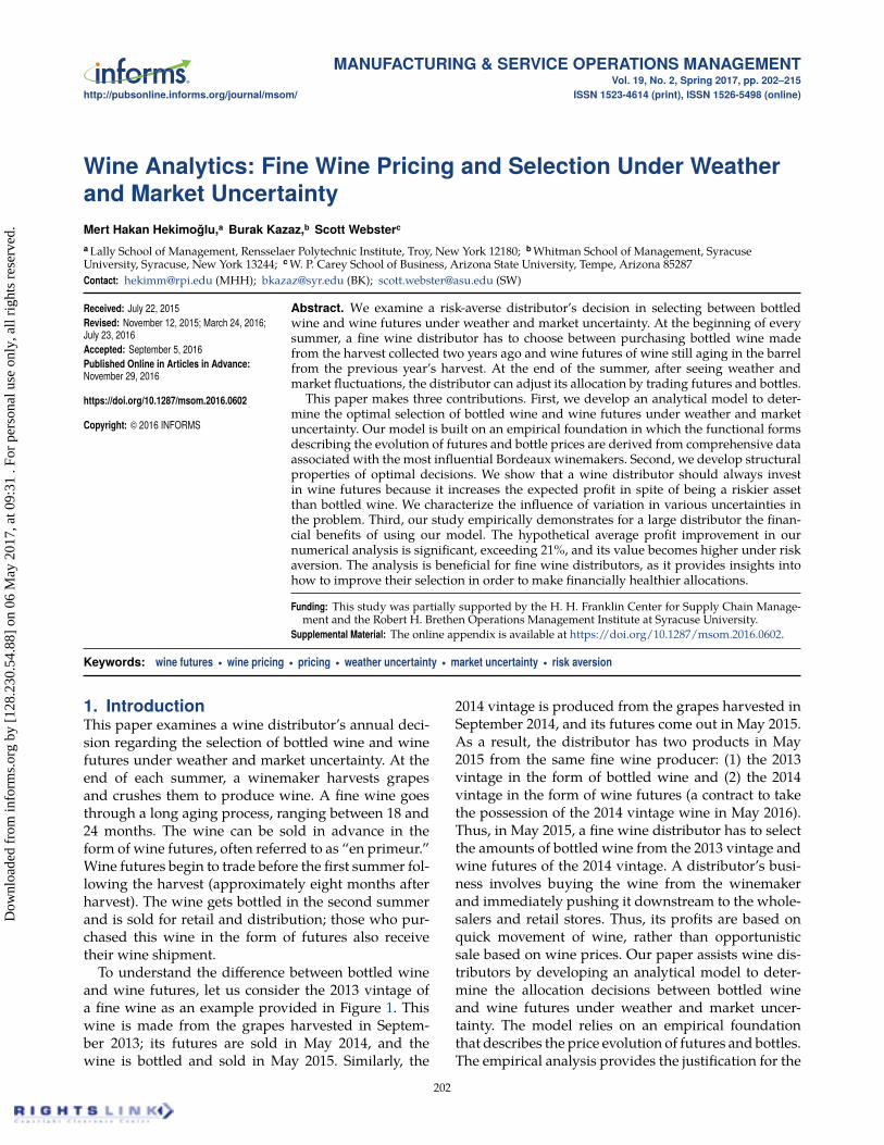
and wine futures, let us consider the 2013 vintage ofa fine wine as an example provided in Figure 1. Thiswine is made from the grapes harvested in Septem-ber 2013; its futures are sold in May 2014, and thewine is bottled and sold in May 2015. Similarly, the
2014 vintage is produced from the grapes harvested inSeptember 2014, and its futures come out in May 2015.As a result, the distributor has two products in May2015 from the same fine wine producer: (1) the 2013vintage in the form of bottled wine and (2) the 2014vintage in the form of wine futures (a contract to takethe possession of the 2014 vintage wine in May 2016).Thus, in May 2015, a fine wine distributor has to selectthe amounts of bottled wine from the 2013 vintage andwine futures of the 2014 vintage. A distributor’s busi-ness involves buying the wine from the winemakerand immediately pushing it downstream to the whole-salers and retail stores. Thus, its profits are based onquick movement of wine, rather than opportunisticsale based on wine prices. Our paper assists wine dis-tributors by developing an analytical model to deter-mine the allocation decisions between bottled wineand wine futures under weather and market uncer-tainty. The model relies on an empirical foundationthat describes the price evolution of futures and bottles.The empirical analysis provides the justification for the
202
Dow
nloa
ded
from
info
rms.
org
by [
128.
230.
54.8
8] o
n 06
May
201
7, a
t 09:
31 .
For
pers
onal
use
onl
y, a
ll ri
ghts
res
erve
d.
Hekimoğlu, Kazaz, and Webster: Wine Pricing and Selection Under Weather and Market UncertaintyManufacturing & Service Operations Management, 2017, vol. 19, no. 2, pp. 202–215, ©2016 INFORMS 203
Figure 1. (Color online) The Timeline of Futures and Bottle Trade in Wine ProductionSeptember 2013 May 2014 September 2014 May 2015
Harvesting2013 vintage
Wine futures2013 vintage
Harvesting2014 vintage
Bottled wine2013 vintage
Wine futures2014 vintage
functional forms describing the impact of weather andmarket conditions on prices.Quality of a fine wine is greatly influenced by
weather conditions during the grape growing season;often higher temperatures lead to better quality ofgrapes and wine. Because of differences in weatherconditions from one year to the other, two consecu-tive vintages of the same wine may have very differentquality, and hence, price. A striking example regardingthe impact of weather on wine futures prices can beseen from the Bordeaux region, where the summer of2005 was very hot and dry, resulting in one of the finestvintages in recent years. Prior to the growing seasonin 2005, the wine futures for the 2004 vintage of Trop-long Mondot were released to the market at the priceof $62/bottle. The impact of superior weather in thesummer of 2005 was so big that the wine futures pricefor the 2005 Troplong Mondot jumped to $233/bottle,a 276% increase. This is an example of the improvedweather conditions from 2004 to 2005 and its impacton wine futures prices. Moreover, the positive weatherduring the summer of 2005 negatively impacted the2004 vintage wine and caused the bottle price of thatvintage to go down to $54 per bottle, a 13% reduc-tion from its futures price from the prior year. Thisis an example where the growing weather conditionsnot only influence the wine futures price but also theevolution of a futures price to the bottle price in theprevious vintage.
In addition to weather fluctuations, changes in themarket conditions also drive fine wine prices. All finewine futures and bottles are traded in London Inter-national Vintner’s Exchange (Liv-ex) with standard-ized contracts. We use Liv-ex 100 index, composedof the 100 most sought-after wines, to describe thefine wine market conditions. Reuters calls this indexthe “fine wine industry’s leading benchmark.” WhenLiv-ex 100 index decreased by 17.17% in 2008 (in com-parison to 2007), the top Bordeaux winemakers pricedtheir 2008 vintage wines 16.66% lower than their 2007vintage wines on average, despite the highly simi-lar weather conditions between the two growing sea-sons. Our analysis combines the impact of weather andmarket fluctuations in explaining the price evolutionof wine futures and bottled wine. These price evolu-tion functions are utilized in developing an analytical
model to help the distributor’s selection between winefutures and bottled wine.
Wine distribution is an important business aroundthe world. In the United States alone, the wine indus-try is expected to generate $38.9 billion in 2016, witha projected annual growth ranging between 9–13% inthe upcoming five years. Under the presence of drasticchanges in vintage prices, depending on weather andmarket conditions, a wine distributor is often puzzledabout whether to invest in wine futures of the previ-ous year’s vintage or to buy recently bottled wine fromtwo vintages ago. While wine futures exhibit a greateruncertainty, as future weather conditions can nega-tively influence the bottle price, as in the example of the2004 Troplong Mondot, they also allow the distributorto lock up limited supply at lower prices. Moreover,futures can be easily traded in Liv-ex, the exchangeplatform for fine wine, without having to make physi-cal shipments and comply with legal restrictions. Thus,wine futures are highly liquid in comparison to bottledwine. Purchasing bottles can be perceived as a saferbet up front as the bottle prices are revealed. However,market conditions continue to influence these prices.The distributor can observe the summer weather con-ditions and get comparative indications as to how thefutures price is going to evolve to the bottle price.Moreover, the distributor can later change its allocationby buying additional or selling existing futures, withlimited ability to move its bottled wine inventory.
When should a wine distributor engage in futures?Our work finds motivation from conversations withthe executives at the largest wine distributor in theUnited States and in the world that does not invest inwine futures because of the lack of knowledge aboutfutures prices and their evolution to bottle prices. Ear-lier research (Ashenfelter et al. 1995, Ashenfelter 2008)has shown that mature Bordeaux wine prices can bepredicted accurately using growing season weatherconditions, but these studies conclude that youngwineprices (i.e., futures prices and prices for the recentlyreleased bottled wines) cannot be predicted usingweather conditions. Our empirical analysis providesan explanation for the impact of weather and mar-ket changes in young wine prices. It serves as a foun-dation for our analytical model, and enables us to
Dow
nloa
ded
from
info
rms.
org
by [
128.
230.
54.8
8] o
n 06
May
201
7, a
t 09:
31 .
For
pers
onal
use
onl
y, a
ll ri
ghts
res
erve
d.
Hekimoğlu, Kazaz, and Webster: Wine Pricing and Selection Under Weather and Market Uncertainty204 Manufacturing & Service Operations Management, 2017, vol. 19, no. 2, pp. 202–215, ©2016 INFORMS
estimate the distributor’s economic benefit from invest-ing in a combination of wine futures and bottled wine(when compared with a distributor that invests only inbottled wine).Wine futures are often perceived to be a riskier
alternative than bottled wine. Our empirical analy-sis confirms this perception, as it shows that pricesfor wine futures are influenced by both weather andmarket fluctuations, whereas bottled wine prices areinfluenced only by the changes in market conditions.Thus, a distributor would not be encouraged to makeinvestments in futures. Rather, the distributor wouldspend its money on physical bottles where the price isalready evolved and has smaller uncertainty. Indeed,this has been the practice at some distributors thatinvest solely in bottled wine, bypassing the futuresalternative. Our analytical model shows, however, thata distributor should always make some investment infutures. This finding is confirmed through a numericalanalysis using comprehensive data.
The remainder of the paper is organized as fol-lows. Section 2 reviews the relevant literature from ec-onomics, operations, and supply chain managementand demonstrates how our work differs from earlierpublications. Section 3 develops an analytical modelto help a distributor determine the allocation deci-sions between wine futures and bottled wine. Sec-tion 4 presents the economic benefit from our proposedmodel using comprehensive data from the most influ-ential Bordeaux winemakers. Section 5 presents ourconclusions and managerial insights. All proofs andderivations, and the details of our data collection arepresented in the online appendix.
2. Literature ReviewThe economics literature has shown significant inter-est in understanding, explaining, and predicting wineprices. Ashenfelter et al. (1995 and 2008) have two sem-inal papers showing that mature Bordeaux wine pricescan be predicted using weather and age with accuracy;however, both studies conclude that their models fail toexplain youngwine prices. For awine distributor, how-ever, most trade takes place when the wine is young;it is therefore important to understand the evolutionof young wine prices. Our work examines how youngwine prices are impacted by the fluctuations inweatherand market conditions. While we complete this anal-ysis to build an analytical model that determines theoptimal selection of wine futures and bottled wine, ourempirical findings complement earlier publications byproviding an explanation for the evolution of youngwine prices.
Jones and Storchmann (2001), Lecocq and Visser(2006), Ali and Nauges (2007), Ali et al. (2008), andAshenfelter and Jones (2013) also address the price pre-diction of Bordeauxwines based onweather conditions
and/or tasting scores. Byron and Ashenfelter (1995)and Wood and Anderson (2006) extend this streamto Australian wines, while Haeger and Storchmann(2006) andAshenfelter and Storchmann (2010) examineAmerican and German wines, respectively. However,none of these papers focuses on young wine pricing orhave a selection analysis that can benefit distributors.
Noparumpa et al. (2015) investigate the impact oftasting scores on young wine prices and providea model for winemakers to determine the optimalamount of wine to be sold in the form of futures andthe optimal amount that should be sold after the wineis bottled. Their work concludes that wine futures helpa winemaker collect revenues in advance and pass therisk of having a poor quality vintage to the distributor.They estimate that selling wine in advance in the formof futures increases Bordeaux winemakers’ profits by10% on average. If winemakers are the clear winnersof futures trade, then one asks what is in it for thewine distributors. Our paper sheds light on this ques-tion by providing an analytical model that incorporatesthe advantages (i.e., being easily tradable through theLiv-ex platform) and the disadvantages (i.e., bearinga greater price uncertainty) of wine futures for dis-tributors. We utilize weather and market fluctuationsinstead of tasting scores (correlated with weather) toexplain futures prices; this leads to considerably higherexplaining power with greater adjusted R2 values ina larger sample featuring the leading Bordeaux wine-makers. Moreover, our explanation of the evolution ofa futures price into bottle price is a unique aspect ofour study.
Wine futures is a form of advance selling and pur-chasing, and recent publications advocate the use ofadvance selling in various settings. Xie and Shugan(2001) exemplify the benefits in electronic tickets andonline platforms. Cho and Tang (2013) examine theinfluence of supply and demand uncertainty, and Tangand Lim (2013) investigate the influence of speculatorsin advance selling. Boyacı andÖzer (2010) demonstratethe advantages of advance selling in capacity planning.Our work departs from these studies in three features:(1) the wine distributor has to choose between advancepurchase of an upcoming product in replacement ofthe present product; (2) as the price evolves throughrevelations of uncertainty, the distributor has the abil-ity to adjust its selection between the two product offer-ings; (3) the sources of uncertainty in our problem areweather and market fluctuations, differentiating ourproblem setting.
Wine futures depart from the commodity futures de-scribed in Fama and French (1987) and Geman (2005).In commodity markets (e.g., corn, soybean, cocoa), asettlement in a futures contract means that the agri-cultural product delivered to the buyer can be pro-duced by any farmer. In fine wine, however, if a buyer
Dow
nloa
ded
from
info
rms.
org
by [
128.
230.
54.8
8] o
n 06
May
201
7, a
t 09:
31 .
For
pers
onal
use
onl
y, a
ll ri
ghts
res
erve
d.
Hekimoğlu, Kazaz, and Webster: Wine Pricing and Selection Under Weather and Market UncertaintyManufacturing & Service Operations Management, 2017, vol. 19, no. 2, pp. 202–215, ©2016 INFORMS 205
is asking for a bottle of 2008 Lafite Rothschild, theseller cannot substitute it with a bottle of 2007 LafiteRothschild, or a bottle of 2008 Troplong Mondot. Thus,fine wine cannot be substituted across producers orvintages and therefore is not a commodity. Moreover,in traditional commodities, futures contracts and spotpurchases occur simultaneously for the commodityproduct. However, spot purchases of bottled fine winedo not begin until the completion of the futures tradeof the same wine.Fine wines are also treated as a long-term invest-
ment. Storchmann (2012) provides a comprehensivereview about wine economics and covers the use ofwine as an investment option. Dimson et al. (2014) findthat young Bordeaux wines yield greater returns thanmature ones. This finding further amplifies the impor-tance of explaining the evolution of young wine prices.Jaeger (1981), Burton and Jacobsen (2001), and MassetandWeisskopf (2010) also examine the return onwinesas a long-term investment. Jaeger (1981), Burton andJacobsen (2001), and Dimson et al. (2014) conclude thatwines can yield greater returns than Treasury bills, butless than equities. Masset andWeisskopf (2010), in con-trast, demonstrate that finewines can outperform equi-ties during a financial crisis when financial assets arehighly correlated. While these studies consider wine asa long-term investment, our paper focuses on its ben-efits as a short-term investment from the perspectiveof a distributor who buys the recently released youngwines from winemakers and sells to wholesalers andretailers shortly after.
Supply uncertainty is another related stream, asquality and price may vary dramatically across differ-ent vintages of the same wine, depending on weatherand market conditions. Yano and Lee (1995) providea comprehensive review of the literature that focuseson supply uncertainty as a consequence of yield fluc-tuations. Jones et al. (2001) examine the impact ofyield uncertainty in the corn seed industry for a firmthat utilizes farmland in two opposing hemispheres;they develop a two-stage production scheme to bettermatch supply and demand. Kazaz (2004) introducesthe impact of yield fluctuations into what he definesas the yield-dependent cost and price structures in theolive oil industry. Kazaz and Webster (2011) add aprice-setting capability and show how yield fluctua-tions influence a firm’s pricing decisions. Their studyalso demonstrates the benefits of using fruit futures(if they exist) in mitigating supply uncertainty. Boy-abatlı et al. (2011) and Boyabatlı (2015) examine thepurchasing contracts for fixed-proportion technologyproducts in the presence of random spot prices. KazazandWebster (2015) develop optimal price and quantitydecisions under supply and demand uncertainty andunder risk aversion. Tomlin and Wang (2008) developprice and quantity decisions in a coproduction setting
that results from random yield in the split of two dis-tinct products. Li and Huh (2011) also develop priceand quantity decisions for multiple products using amultinomial logit model.
Departing from these papers, we define supply un-certainty in the form of variation in quality due togrowing season weather; hence, wine futures havea quality-dependent price structure. Moreover, thesecondary (emergency) investment option utilized insome of these papers becomes available in the sec-ond stage, whereas in our model, both wine futuresand bottled wines are simultaneously available at thebeginning.
Weather and market realizations provide signalsto the wine industry, and the impact of similar sig-nals, in particular for estimating demand, is exam-ined widely in the operations management literature.Gümüş (2014), for example, investigates the impact offorecast as a signal for demand. Our work departs fromthis body of literature as we study signals that influ-ence the evolution of price over time.
3. The Model and Its AnalysisThis section develops and analyzes a model that helpsthe wine distributor determine an investment alloca-tion between wine futures and bottled wine. The pricesof wine futures and bottled wine are influenced by therandomness in weather and market conditions afterthese decisions take place. In this model, the functionalforms describing the evolution of futures and bottleprices rely on an empirical foundation.
Each May, a risk-averse wine distributor has to selectbetween wine futures (of new vintage) and bottledwine (of previous vintage). Specifically, in May of cal-endar year t, the distributor has to determine theamount of money to invest in wine futures from vin-tage t − 1 and bottled wine from vintage t − 2.
3.1. Empirical Foundation for the ModelIn this section, we present an empirical analysis thatserves as a foundation for the mathematical model thatwe present in Section 3.2. The results of our empiricalanalysis determine the functional forms describing theprice evolution of young wines as functions of weatherand random market variables. The functional formsthat emerge from the empirical analysis are used in theanalytical model.
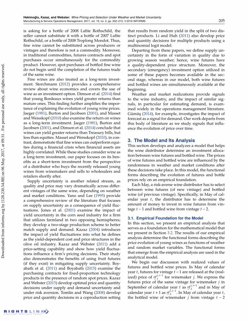
We begin our discussion with realized values offutures and bottled wine prices. In May of calendaryear t, futures for vintage t−1 are released at the (real-ized) price of rf j, t−1
1 for winemaker j. We express thefutures price of the same vintage for winemaker j inSeptember of calendar year t as rf j, t−1
2 and in May ofcalendar year t + 1 as rf j, t−1
3 . In May of calendar year t,the bottled wine of winemaker j from vintage t − 2
Dow
nloa
ded
from
info
rms.
org
by [
128.
230.
54.8
8] o
n 06
May
201
7, a
t 09:
31 .
For
pers
onal
use
onl
y, a
ll ri
ghts
res
erve
d.
Hekimoğlu, Kazaz, and Webster: Wine Pricing and Selection Under Weather and Market Uncertainty206 Manufacturing & Service Operations Management, 2017, vol. 19, no. 2, pp. 202–215, ©2016 INFORMS
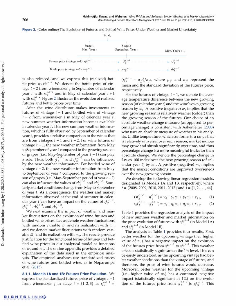
Figure 2. (Color online) The Evolution of Futures and Bottled Wine Prices Under Weather and Market Uncertaintywt , mt˜
Stage 1May, Year t
Stage 2September, Year t May, Year t + 1
Futures price (vintage t–1): rf1j, t–1
Bottle price (vintage t–2): rb1j, t–2
rf2j, t–1 rf
3j, t–1
rb2j, t–2 rb
3j, t–2
˜
is also released, and we express this (realized) bot-tle price as rb j, t−2
1 . We denote the bottle price of vin-tage t − 2 from winemaker j in September of calendaryear t with rb j, t−2
2 and in May of calendar year t + 1with rb j, t−2
3 . Figure 2 illustrates the evolution of realizedfutures and bottle prices over time.After the wine distributor makes investments in
futures of vintage t − 1 and bottled wine of vintaget − 2 from winemaker j in May of calendar year t,new summer weather information becomes availablein calendar year t. This new summer weather informa-tion, which is fully observed by September of calendaryear t, provides a relative comparison to the wines thatare from vintages t − 1 and t − 2. For wine futures ofvintage t − 1, the new weather information from Mayto September of year t compared to the growing seasonof grapes (i.e., May–September of year t − 1) can playa role. Thus, both rf j, t−1
2 and rf j, t−13 can be influenced
by the new weather information. For bottled wine ofvintage t − 2, the new weather information from Mayto September of year t compared to the growing sea-son of grapes (i.e., May–September period of year t−2)can also influence the values of rb j, t−2
2 and rb j, t−23 . Simi-
larly, market conditions change fromMay to Septemberof year t. As a consequence, the weather and marketinformation observed at the end of summer in calen-dar year t can have an impact on the values of rf j, t−1
2 ,rf j, t−1
3 , rb j, t−22 , and rb j, t−2
3 .We next examine the impact of weather and mar-
ket fluctuations on the evolution of wine futures andbottled wine prices. Let us denote weather fluctuationswith random variable wt and its realization with wt ,and we denote market fluctuations with random vari-able mt and its realization with mt . The results providejustification for the functional forms of futures and bot-tled wine prices in our analytical model as functionsof wt and mt . The online appendix provides a detailedexplanation of the data used in the empirical anal-ysis. The empirical analyses use standardized pricesof wine futures and bottled wine, as in Noparumpaet al. (2015).
3.1.1. Models 1A and 1B: Futures Price Evolution. Weexpress the standardized futures price of vintage t − 1from winemaker j in stage i 1, 2, 3 as sf j, t−1
i
(rf j,t−1i − µ f j
i)/σ f j
i, where µ f j
iand σ f j
irepresent the
mean and the standard deviation of the futures price,respectively.
For the futures of vintage t − 1, we denote the aver-age temperature difference between the new growingseason (of calendar year t) and thewine’s own growingseason by wt . A positive (negative) wt implies that thenew growing season is relatively warmer (colder) thanthe growing season of the futures. Our choice of anabsolute weather change measure (as opposed to per-centage change) is consistent with Ashenfelter (2008)who uses an absolute measure of weather in his analy-sis. Unlike temperature, which conforms to a range thatis relatively universal over each season, market indicesmay grow and shrink significantly over time, and thuspercentage change is a more meaningful indicator thanabsolute change. We denote the percentage change inLiv-ex 100 index over the new growing season (of cal-endar year t) by mt . A positive (negative) mt impliesthat the market conditions are improved (worsened)over the new growing season.
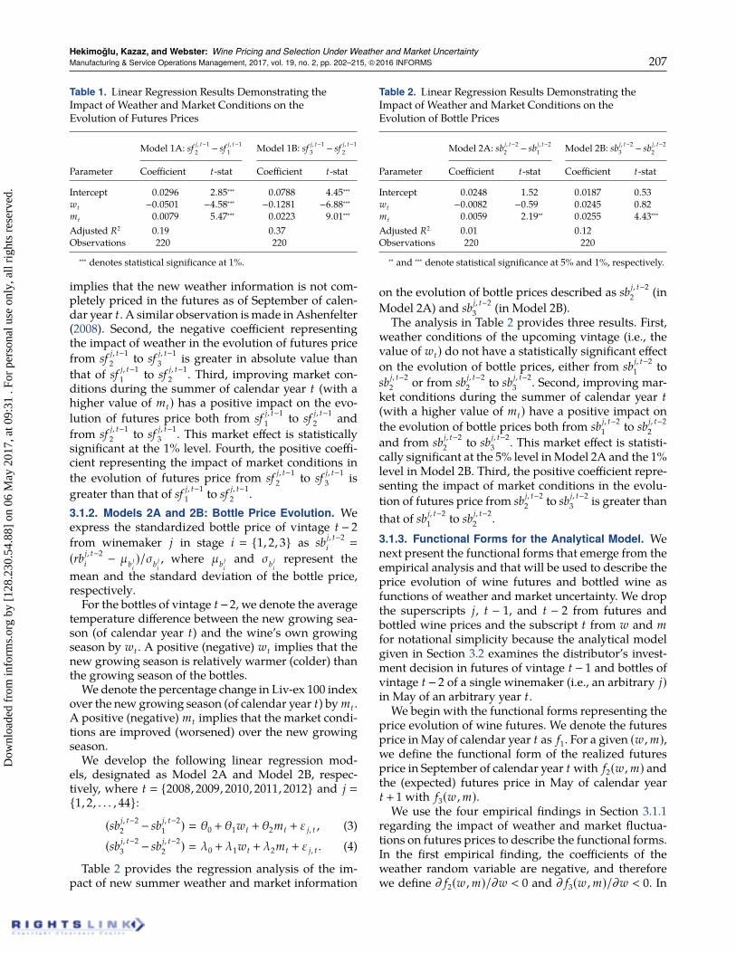
We develop the following linear regression models,designated as Models 1A and 1B, respectively, wheret 2008, 2009, 2010, 2011, 2012 and j 1, 2, . . . , 44:
(sf j, t−12 − sf j, t−1
1 ) γ0 + γ1wt + γ2mt + ε j, t , (1)(sf j, t−1
3 − sf j, t−12 ) η0 + η1wt + η2mt + ε j, t . (2)
Table 1 provides the regression analysis of the impactof new summer weather and market information onthe price evolution of futures with sf j, t−1
2 (in Model 1A)and sf j, t−1
3 (in Model 1B).The analysis in Table 1 provides four results. First,
better weather for the upcoming vintage (i.e., highervalue of wt) has a negative impact on the evolutionof the futures price from sf j, t−1
1 to sf j, t−12 . This weather
effect is statistically significant at the 1% level. This canbe easily understood, as the upcoming vintage had bet-ter weather conditions than the vintage of futures, andtherefore, the price of wine futures would decrease.Moreover, better weather for the upcoming vintage(i.e., higher value of wt) has a continued negativeimpact (statistically significant at 1%) on the evolu-tion of the futures price from sf j, t−1
2 to sf j, t−13 . This
Dow
nloa
ded
from
info
rms.
org
by [
128.
230.
54.8
8] o
n 06
May
201
7, a
t 09:
31 .
For
pers
onal
use
onl
y, a
ll ri
ghts
res
erve
d.
Hekimoğlu, Kazaz, and Webster: Wine Pricing and Selection Under Weather and Market UncertaintyManufacturing & Service Operations Management, 2017, vol. 19, no. 2, pp. 202–215, ©2016 INFORMS 207
Table 1. Linear Regression Results Demonstrating theImpact of Weather and Market Conditions on theEvolution of Futures Prices
Model 1A: sf j, t−12 − sf j, t−1
1 Model 1B: sf j, t−13 − sf j, t−1
2
Parameter Coefficient t-stat Coefficient t-stat
Intercept 0.0296 2.85∗∗∗ 0.0788 4.45∗∗∗wt −0.0501 −4.58∗∗∗ −0.1281 −6.88∗∗∗mt 0.0079 5.47∗∗∗ 0.0223 9.01∗∗∗
Adjusted R2 0.19 0.37Observations 220 220∗∗∗ denotes statistical significance at 1%.
implies that the new weather information is not com-pletely priced in the futures as of September of calen-dar year t. A similar observation ismade inAshenfelter(2008). Second, the negative coefficient representingthe impact of weather in the evolution of futures pricefrom sf j, t−1
2 to sf j, t−13 is greater in absolute value than
that of sf j, t−11 to sf j, t−1
2 . Third, improving market con-ditions during the summer of calendar year t (with ahigher value of mt) has a positive impact on the evo-lution of futures price both from sf j, t−1
1 to sf j, t−12 and
from sf j, t−12 to sf j, t−1
3 . This market effect is statisticallysignificant at the 1% level. Fourth, the positive coeffi-cient representing the impact of market conditions inthe evolution of futures price from sf j, t−1
2 to sf j, t−13 is
greater than that of sf j, t−11 to sf j, t−1
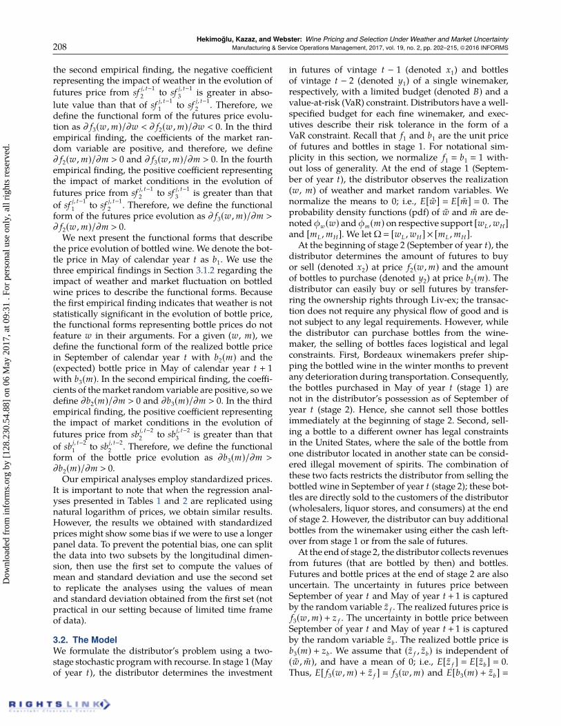
2 .3.1.2. Models 2A and 2B: Bottle Price Evolution. Weexpress the standardized bottle price of vintage t − 2from winemaker j in stage i 1, 2, 3 as sb j, t−2
i
(rb j, t−2i − µb j
i)/σb j
i, where µb j
iand σb j
irepresent the
mean and the standard deviation of the bottle price,respectively.For the bottles of vintage t−2, we denote the average
temperature difference between the new growing sea-son (of calendar year t) and the wine’s own growingseason by wt . A positive (negative) wt implies that thenew growing season is relatively warmer (colder) thanthe growing season of the bottles.We denote the percentage change in Liv-ex 100 index
over the new growing season (of calendar year t) by mt .A positive (negative) mt implies that the market condi-tions are improved (worsened) over the new growingseason.We develop the following linear regression mod-
els, designated as Model 2A and Model 2B, respec-tively, where t 2008, 2009, 2010, 2011, 2012 and j 1, 2, . . . , 44:
(sb j, t−22 − sb j, t−2
1 ) θ0 + θ1wt + θ2mt + ε j, t , (3)(sb j, t−2
3 − sb j, t−22 ) λ0 + λ1wt + λ2mt + ε j, t . (4)
Table 2 provides the regression analysis of the im-pact of new summer weather and market information
Table 2. Linear Regression Results Demonstrating theImpact of Weather and Market Conditions on theEvolution of Bottle Prices
Model 2A: sb j, t−22 − sb j, t−2
1 Model 2B: sb j, t−23 − sb j, t−2
2
Parameter Coefficient t-stat Coefficient t-stat
Intercept 0.0248 1.52 0.0187 0.53wt −0.0082 −0.59 0.0245 0.82mt 0.0059 2.19∗∗ 0.0255 4.43∗∗∗
Adjusted R2 0.01 0.12Observations 220 220∗∗ and ∗∗∗ denote statistical significance at 5% and 1%, respectively.
on the evolution of bottle prices described as sb j, t−22 (in
Model 2A) and sb j, t−23 (in Model 2B).
The analysis in Table 2 provides three results. First,weather conditions of the upcoming vintage (i.e., thevalue of wt) do not have a statistically significant effecton the evolution of bottle prices, either from sb j, t−2
1 tosb j, t−2
2 or from sb j, t−22 to sb j, t−2
3 . Second, improving mar-ket conditions during the summer of calendar year t(with a higher value of mt) have a positive impact onthe evolution of bottle prices both from sb j, t−2
1 to sb j, t−22
and from sb j, t−22 to sb j, t−2
3 . This market effect is statisti-cally significant at the 5% level inModel 2A and the 1%level in Model 2B. Third, the positive coefficient repre-senting the impact of market conditions in the evolu-tion of futures price from sb j, t−2
2 to sb j, t−23 is greater than
that of sb j, t−21 to sb j, t−2
2 .3.1.3. Functional Forms for the Analytical Model. Wenext present the functional forms that emerge from theempirical analysis and that will be used to describe theprice evolution of wine futures and bottled wine asfunctions of weather and market uncertainty. We dropthe superscripts j, t − 1, and t − 2 from futures andbottled wine prices and the subscript t from w and mfor notational simplicity because the analytical modelgiven in Section 3.2 examines the distributor’s invest-ment decision in futures of vintage t − 1 and bottles ofvintage t − 2 of a single winemaker (i.e., an arbitrary j)in May of an arbitrary year t.
We begin with the functional forms representing theprice evolution of wine futures. We denote the futuresprice inMay of calendar year t as f1. For a given (w ,m),we define the functional form of the realized futuresprice in September of calendar year t with f2(w ,m) andthe (expected) futures price in May of calendar yeart + 1 with f3(w ,m).We use the four empirical findings in Section 3.1.1
regarding the impact of weather and market fluctua-tions on futures prices to describe the functional forms.In the first empirical finding, the coefficients of theweather random variable are negative, and thereforewe define ∂ f2(w ,m)/∂w < 0 and ∂ f3(w ,m)/∂w < 0. In
Dow
nloa
ded
from
info
rms.
org
by [
128.
230.
54.8
8] o
n 06
May
201
7, a
t 09:
31 .
For
pers
onal
use
onl
y, a
ll ri
ghts
res
erve
d.
Hekimoğlu, Kazaz, and Webster: Wine Pricing and Selection Under Weather and Market Uncertainty208 Manufacturing & Service Operations Management, 2017, vol. 19, no. 2, pp. 202–215, ©2016 INFORMS
the second empirical finding, the negative coefficientrepresenting the impact of weather in the evolution offutures price from sf j, t−1
2 to sf j, t−13 is greater in abso-
lute value than that of sf j, t−11 to sf j, t−1
2 . Therefore, wedefine the functional form of the futures price evolu-tion as ∂ f3(w ,m)/∂w < ∂ f2(w ,m)/∂w < 0. In the thirdempirical finding, the coefficients of the market ran-dom variable are positive, and therefore, we define∂ f2(w ,m)/∂m > 0 and ∂ f3(w ,m)/∂m > 0. In the fourthempirical finding, the positive coefficient representingthe impact of market conditions in the evolution offutures price from sf j, t−1
2 to sf j, t−13 is greater than that
of sf j, t−11 to sf j, t−1
2 . Therefore, we define the functionalform of the futures price evolution as ∂ f3(w ,m)/∂m >∂ f2(w ,m)/∂m > 0.We next present the functional forms that describe
the price evolution of bottled wine. We denote the bot-tle price in May of calendar year t as b1. We use thethree empirical findings in Section 3.1.2 regarding theimpact of weather and market fluctuation on bottledwine prices to describe the functional forms. Becausethe first empirical finding indicates that weather is notstatistically significant in the evolution of bottle price,the functional forms representing bottle prices do notfeature w in their arguments. For a given (w, m), wedefine the functional form of the realized bottle pricein September of calendar year t with b2(m) and the(expected) bottle price in May of calendar year t + 1with b3(m). In the second empirical finding, the coeffi-cients of themarket randomvariable are positive, sowedefine ∂b2(m)/∂m > 0 and ∂b3(m)/∂m > 0. In the thirdempirical finding, the positive coefficient representingthe impact of market conditions in the evolution offutures price from sb j, t−2
2 to sb j, t−23 is greater than that
of sb j, t−21 to sb j, t−2
2 . Therefore, we define the functionalform of the bottle price evolution as ∂b3(m)/∂m >∂b2(m)/∂m > 0.Our empirical analyses employ standardized prices.
It is important to note that when the regression anal-yses presented in Tables 1 and 2 are replicated usingnatural logarithm of prices, we obtain similar results.However, the results we obtained with standardizedprices might show some bias if we were to use a longerpanel data. To prevent the potential bias, one can splitthe data into two subsets by the longitudinal dimen-sion, then use the first set to compute the values ofmean and standard deviation and use the second setto replicate the analyses using the values of meanand standard deviation obtained from the first set (notpractical in our setting because of limited time frameof data).
3.2. The ModelWe formulate the distributor’s problem using a two-stage stochastic programwith recourse. In stage 1 (Mayof year t), the distributor determines the investment
in futures of vintage t − 1 (denoted x1) and bottlesof vintage t − 2 (denoted y1) of a single winemaker,respectively, with a limited budget (denoted B) and avalue-at-risk (VaR) constraint. Distributors have a well-specified budget for each fine winemaker, and exec-utives describe their risk tolerance in the form of aVaR constraint. Recall that f1 and b1 are the unit priceof futures and bottles in stage 1. For notational sim-plicity in this section, we normalize f1 b1 1 with-out loss of generality. At the end of stage 1 (Septem-ber of year t), the distributor observes the realization(w, m) of weather and market random variables. Wenormalize the means to 0; i.e., E[w] E[m] 0. Theprobability density functions (pdf) of w and m are de-noted φw(w) and φm(m) on respective support [wL ,wH]and [mL ,mH]. We let Ω [wL ,wH] × [mL ,mH].
At the beginning of stage 2 (September of year t), thedistributor determines the amount of futures to buyor sell (denoted x2) at price f2(w ,m) and the amountof bottles to purchase (denoted y2) at price b2(m). Thedistributor can easily buy or sell futures by transfer-ring the ownership rights through Liv-ex; the transac-tion does not require any physical flow of good and isnot subject to any legal requirements. However, whilethe distributor can purchase bottles from the wine-maker, the selling of bottles faces logistical and legalconstraints. First, Bordeaux winemakers prefer ship-ping the bottled wine in the winter months to preventany deterioration during transportation. Consequently,the bottles purchased in May of year t (stage 1) arenot in the distributor’s possession as of September ofyear t (stage 2). Hence, she cannot sell those bottlesimmediately at the beginning of stage 2. Second, sell-ing a bottle to a different owner has legal constraintsin the United States, where the sale of the bottle fromone distributor located in another state can be consid-ered illegal movement of spirits. The combination ofthese two facts restricts the distributor from selling thebottled wine in September of year t (stage 2); these bot-tles are directly sold to the customers of the distributor(wholesalers, liquor stores, and consumers) at the endof stage 2. However, the distributor can buy additionalbottles from the winemaker using either the cash left-over from stage 1 or from the sale of futures.
At the end of stage 2, the distributor collects revenuesfrom futures (that are bottled by then) and bottles.Futures and bottle prices at the end of stage 2 are alsouncertain. The uncertainty in futures price betweenSeptember of year t and May of year t + 1 is capturedby the random variable z f . The realized futures price isf3(w ,m) + z f . The uncertainty in bottle price betweenSeptember of year t and May of year t + 1 is capturedby the random variable zb . The realized bottle price isb3(m) + zb . We assume that (z f , zb) is independent of(w , m), and have a mean of 0; i.e., E[z f ] E[zb] 0.Thus, E[ f3(w ,m) + z f ] f3(w ,m) and E[b3(m) + zb]
Dow
nloa
ded
from
info
rms.
org
by [
128.
230.
54.8
8] o
n 06
May
201
7, a
t 09:
31 .
For
pers
onal
use
onl
y, a
ll ri
ghts
res
erve
d.
Hekimoğlu, Kazaz, and Webster: Wine Pricing and Selection Under Weather and Market UncertaintyManufacturing & Service Operations Management, 2017, vol. 19, no. 2, pp. 202–215, ©2016 INFORMS 209
b3(m). By examining our price data, we observe that ifthe futures (bottle) price moves in one direction whenit evolves from f1 to f2(w ,m) (from b1 to b2(m)), then awide majority of realized futures (bottle) prices at theend of stage 2 move in the same direction when theyevolve from f2(w ,m) to f3(w ,m) + z f (from b2(m) tob3(m) + zb). We insert the following assumptions thatcomply with this observation:
If f2(w ,m)♦ f1 , then E[ f3(w ,m)+ z f ]♦ f2(w ,m),for all ♦ ∈ >,, < and for all (w ,m). (5)
If b2(m)♦ b1 , then E[b3(m)+ zb]♦ b2(m),for all ♦ ∈ >,, < and for all m. (6)
All price functions f2(w ,m), f3(w ,m), b2(m), andb3(m) are linear in their arguments and are net of trans-action, shipping, and other Costs; i.e., the prices reflectthe net revenues in these two stages. Thus, the realizedprofit at the end of stage 2 can be expressed as follows:
Π(x1 , y1 ,w ,m , x2 , y2 , z f , zb)−x1 − y1 − f2(w ,m)x2 − b2(m)y2 + [ f3(w ,m)+ z f ]· (x1 + x2)+ [b3(m)+ zb](y1 + y2). (7)
At the beginning of stage 2, the distributor selects x2and y2 to maximize expected recourse profit subjectto budget and VaR constraints, given the initial invest-ments in futures and bottles (x1 , y1) and the realizedvalues of weather and market random variable (w ,m):
maxx2 , y2
E[Π(x1 , y1 ,w ,m , x2 , y2 , z f , zb)] (8)
s.t. f2(w ,m)x2 + b2(m)y2 ≤ B − x1 − y1 , (9)P[Π(x1 , y1 ,w ,m , x2 , y2 , z f , zb) < −β
]≤ α, (10)
x2 ≥ −x1 , (11)y2 ≥ 0. (12)
Inequality (9) is the second-stage budget constraint; thedistributor can use the remaining budget from stage 1in addition to the money generated through the sale offutures in stage 2 (when x2 < 0). Inequality (10) is thesecond-stage VaR constraint; the distributor requiresthat the probability of loss more than β (<B) is nomorethan α. In otherwords, the probability of realized profitless than −β should not exceed α. Inequality (11) indi-cates that the distributor cannot sell more futures instage 2 than she purchased in stage 1. For given x1, y1,w ,m, we let (x∗2 , y∗2) denote the optimal solution; i.e.,(
x∗2(x1 , y1 ,w ,m ,), y∗2(x1 , y1 ,w ,m ,))
arg maxx2 , y2
E[Π(x1 , y1 ,w ,m , x2 , y2 , z f , zb)
]s.t. (9)–(12).
Let z f α and zbα denote the realizations of z f and zb ,respectively, at fractile α; i.e., P[z f ≤ z f α] P[zb ≤ zbα]
α. We assume that z f α < 0 and zbα < 0, i.e., the fractileparameter is such that the risk-averse decision makerin September of year t is concerned about profit real-izations in May of year t+1 that are below expectation.We also assume that the VaR constraint is satisfied inthe event the distributor invests the entire budget inbottles; i.e.,
(1− b3(mL) − zbα)B < β. (13)
This assumption is consistent with the practice of dis-tributors who invest solely in bottled wine.
At the beginning of stage 1, the distributor selects x1and y1 to maximize expected profit at the end of stage 2subject to budget and VaR constraints:
maxx1 , y1≥0
E[Π(x1 , y1 , w , m , x
∗2(x1 , y1 , w , m),
y∗2(x1 , y1 , w , m), z f , zb)]
(14)s.t. x1 + y1 ≤ B, (15)
P[Π(x1 , y1 ,w ,m , x
∗2(x1 , y1 ,w ,m),
y∗2(x1 , y1 ,w ,m), z f , zb) < −β]≤ α,
for all (w ,m) ∈Ω. (16)
Inequality (15) states that the distributor’s initial invest-ment in futures and bottles cannot exceed the allottedbudget B. Inequality (16) is the VaR constraint under atime-consistent risk measure (e.g., see Boda and Filar2006 or Devalkar et al. 2015). Some first-stage decisions(x1, y1) can satisfy the VaR constraint in stage 1 but maynot comply with the VaR constraint in stage 2; suchdecisions lead to time inconsistency and are not feasi-ble in our model. To assure that risk aversion is timeconsistent over the planning horizon, the distributormust account for the VaR constraint in stage 2, and inparticular, the choice of (x1, y1) must be such that thereexists a solution to the stage-2 problem that satisfiesthe stage-2 VaR constraint for any realization (w, m)of (w , m).We focus on understanding how investment in
futures and bottles affect performance ceteris paribus;therefore, we assume equal and positive expectedreturns at the end of stage 2; i.e.,
E[ f3(w , m)+ z f ] E[b3(m)+ zb] > 1. (17)
We relax this assumption in Section 4.
3.3. AnalysisWe begin our analysis by partitioning the support Ωinto three sets that identify realizations of (w , m),where the distributor would improve expected profitat the end of stage 2 by (1) selling futures, (2) buyingfutures, and (3) selling futures and buying bottles.
Ω0 (w ,m) ∈Ω: f3(w ,m)/ f2(w ,m) b3(m)/b2(m) 1
,
Ω1 (w ,m) ∈Ω: f3(w ,m)/ f2(w ,m) < 1 and
b3(m)/b2(m) < 1,
Dow
nloa
ded
from
info
rms.
org
by [
128.
230.
54.8
8] o
n 06
May
201
7, a
t 09:
31 .
For
pers
onal
use
onl
y, a
ll ri
ghts
res
erve
d.
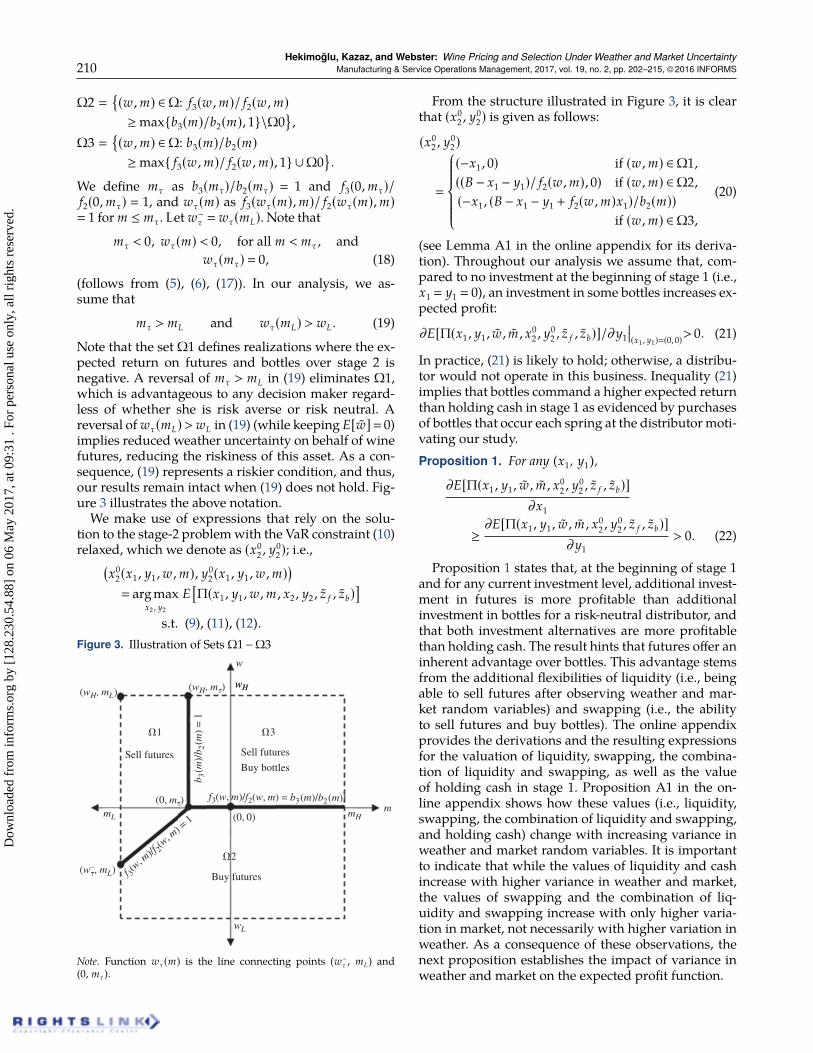
Hekimoğlu, Kazaz, and Webster: Wine Pricing and Selection Under Weather and Market Uncertainty210 Manufacturing & Service Operations Management, 2017, vol. 19, no. 2, pp. 202–215, ©2016 INFORMS
Ω2 (w ,m) ∈Ω: f3(w ,m)/ f2(w ,m)≥maxb3(m)/b2(m), 1\Ω0
,
Ω3 (w ,m) ∈Ω: b3(m)/b2(m)≥max f3(w ,m)/ f2(w ,m), 1 ∪Ω0
.
We define mτ as b3(mτ)/b2(mτ) 1 and f3(0,mτ)/f2(0,mτ) 1, and wτ(m) as f3(wτ(m),m)/ f2(wτ(m),m) 1 for m ≤ mτ. Let w−τ wτ(mL). Note that
mτ < 0, wτ(m) < 0, for all m < mτ , andwτ(mτ) 0, (18)
(follows from (5), (6), (17)). In our analysis, we as-sume that
mτ > mL and wτ(mL) > wL . (19)
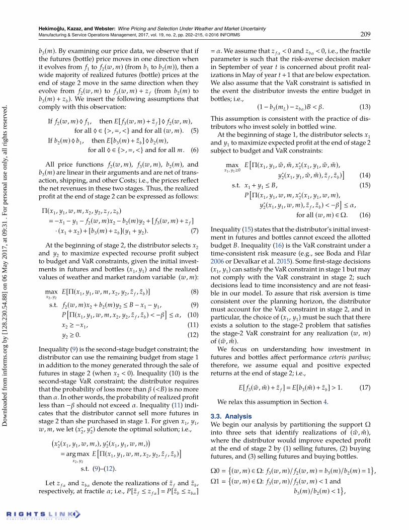
Note that the set Ω1 defines realizations where the ex-pected return on futures and bottles over stage 2 isnegative. A reversal of mτ > mL in (19) eliminates Ω1,which is advantageous to any decision maker regard-less of whether she is risk averse or risk neutral. Areversal of wτ(mL)>wL in (19) (while keeping E[w] 0)implies reduced weather uncertainty on behalf of winefutures, reducing the riskiness of this asset. As a con-sequence, (19) represents a riskier condition, and thus,our results remain intact when (19) does not hold. Fig-ure 3 illustrates the above notation.We make use of expressions that rely on the solu-
tion to the stage-2 problemwith the VaR constraint (10)relaxed, which we denote as (x0
2 , y02); i.e.,(
x02(x1 , y1 ,w ,m), y0
2(x1 , y1 ,w ,m))
arg maxx2 , y2
E[Π(x1 , y1 ,w ,m , x2 , y2 , z f , zb)
]s.t. (9), (11), (12).
Figure 3. Illustration of Sets Ω1−Ω3w
wHwH(wH, m)(wH, mL)
(w– , mL)
1
Sell futures
3
Sell futures
Buy bottles
b 3(m
)/b 2
(m)
= 1
wL
mHm
2
Buy futures
mL
f 3(w
, m)/f 2
(w, m
) = 1
f3(w, m)/f2(w, m) = b3(m)/b2(m)
(0, 0)
(0, m)
Note. Function wτ(m) is the line connecting points (w−τ , mL) and(0, mτ).
From the structure illustrated in Figure 3, it is clearthat (x0
2 , y02) is given as follows:
(x02 , y0
2)
(−x1 , 0) if (w ,m) ∈Ω1,((B − x1 − y1)/ f2(w ,m), 0) if (w ,m) ∈Ω2,(−x1 , (B − x1 − y1 + f2(w ,m)x1)/b2(m))
if (w ,m) ∈Ω3,
(20)
(see Lemma A1 in the online appendix for its deriva-tion). Throughout our analysis we assume that, com-pared to no investment at the beginning of stage 1 (i.e.,x1 y1 0), an investment in some bottles increases ex-pected profit:
∂E[Π(x1 , y1 , w , m , x02 , y
02 , z f , zb)]/∂y1
(x1 , y1)(0,0)
> 0. (21)
In practice, (21) is likely to hold; otherwise, a distribu-tor would not operate in this business. Inequality (21)implies that bottles command a higher expected returnthan holding cash in stage 1 as evidenced by purchasesof bottles that occur each spring at the distributor moti-vating our study.Proposition 1. For any (x1, y1),
∂E[Π(x1 , y1 , w , m , x02 , y0
2 , z f , zb)]∂x1
≥∂E[Π(x1 , y1 , w , m , x0
2 , y02 , z f , zb)]
∂y1> 0. (22)
Proposition 1 states that, at the beginning of stage 1and for any current investment level, additional invest-ment in futures is more profitable than additionalinvestment in bottles for a risk-neutral distributor, andthat both investment alternatives are more profitablethan holding cash. The result hints that futures offer aninherent advantage over bottles. This advantage stemsfrom the additional flexibilities of liquidity (i.e., beingable to sell futures after observing weather and mar-ket random variables) and swapping (i.e., the abilityto sell futures and buy bottles). The online appendixprovides the derivations and the resulting expressionsfor the valuation of liquidity, swapping, the combina-tion of liquidity and swapping, as well as the valueof holding cash in stage 1. Proposition A1 in the on-line appendix shows how these values (i.e., liquidity,swapping, the combination of liquidity and swapping,and holding cash) change with increasing variance inweather and market random variables. It is importantto indicate that while the values of liquidity and cashincrease with higher variance in weather and market,the values of swapping and the combination of liq-uidity and swapping increase with only higher varia-tion in market, not necessarily with higher variation inweather. As a consequence of these observations, thenext proposition establishes the impact of variance inweather and market on the expected profit function.
Dow
nloa
ded
from
info
rms.
org
by [
128.
230.
54.8
8] o
n 06
May
201
7, a
t 09:
31 .
For
pers
onal
use
onl
y, a
ll ri
ghts
res
erve
d.

Hekimoğlu, Kazaz, and Webster: Wine Pricing and Selection Under Weather and Market UncertaintyManufacturing & Service Operations Management, 2017, vol. 19, no. 2, pp. 202–215, ©2016 INFORMS 211
Proposition 2. When φw(w) and φm(m) follow symmetricpdf, (a) E[Π(x1, y1, w, m, x0
2, y02 , z f , zb)] increases in σ2
m;and (b) E[Π(x1 , y1 , w , m , x0
2 , y02 , z f , zb)] increases in σ2
w ifthe combined value from liquidity and swapping increasesin σ2
w .
Proposition 2 shows that, for symmetric distribu-tions, the expected profit increases in σ2
m ; however, itmay increase or decrease in σ2
w . Profit improvementfrom higher variation in market and weather uncer-tainty is enabled because of the recourse flexibility thatallows the distributor to change her futures and bottlesposition based on the realization of the two randomvariables. When the value from the combination of liq-uidity and swapping increases with the variation inweather, then the expected profit also increases withhigher degrees of weather uncertainty.The preceding analysis has focused on the stage-1
profit function for a risk-neutral distributor. We buildon this analysis in our derivation of the optimal solu-tion to the risk-averse distributor problem definedin (8)–(16) in Proposition 3 below. The propositionmakes use of the following notation and inequalities:
x+
1 β
1− f2(wH ,mL),
xV1
β+ zbαB[1− f2(wH ,mτ)][1+ zbα]
,
yV1
β− [1− f2(wH ,mL)]xV1
1− b3(mL) − zbα,
xs1
β− B[1− b3(mL) − zbα]b3(mL)+ zbα − f2(wH ,mL)
,
ys1
B[1− f2(wH ,mL)] − βb3(mL)+ zbα − f2(wH ,mL)
,
−z f α < β/B, (23)
∂E[Π(x1 , y1 , w , m , x02 , y0
2 , z f , zb)]/∂y1 |(x1 , y1)(0,0)
∂E[Π(x1 , y1 , w , m , x02 , y0
2 , z f , zb)]/∂x1 |(x1 ,y1)(0,0)
<1− b3(mL) − zbα
1− f2(wH ,mL). (24)
The value of x+
1 is the number of futures that causeconstraint (16) to be binding (i.e., satisfied exactly) atpoint (wH , mL) given that y1 0. The value of xV
1 isthe number of futures that cause constraint (16) to bebinding (i.e., satisfied exactly) at point (wH , mτ), whichis independent of the value of y1. The value of yV
1 isthe number of bottles that cause constraint (16) to bebinding (i.e., satisfied exactly) at point (wH , mL), giventhat x1 xV
1 . The values of xs1 and ys
1 are the num-bers of futures and bottles, respectively, that cause con-straint (16) at point (wH , mL) to intersect with the bud-get constraint (15). The value of xs
1 is strictly smallerthan x+
1 when x+
1 < B.
Inequality (23) restricts the variation in the random-ness in futures at the end of stage 2. It implies that hav-ing the entire budget invested in futures in stage 2 atpoint (w−τ , mL) does not violate the VaR constraint (10).Note that at point (w−τ , mL), the risk-neutral distributorwould keep all futures and purchase additional futuresif the budget allows. Inequality (23) is a rather mildcondition. Recall (13), which says the VaR constraintis not violated if the distributor uses the entire bud-get to purchase bottles at the beginning of stage 1 (acondition supported by observed practice); i.e., −zbα <β/B−[1− b3(mL)]< β/B. A comparison of (23) with (13)shows that our model allows for greater uncertaintyin the randomness in futures prices than that in bottleprices. Unlike (13), inequality (23) does not mean thatinvesting the entire budget in futures in stage 1 wouldnot violate the VaR constraint (16). Rather, investing theentire budget in futures in stage 1 under (23) may vio-late the VaR constraint (16) at (wH ,mτ) and (wH , mL).
Inequality (24) is used as a condition in charac-terizing the optimal solution. It compares the ratioof marginal returns from bottles to futures with theratio of worst loss from bottles at α-fractile (i.e., 1 −b3(mL) − zbα) to futures (1 − f2(wH ,mL)), because thedistributor can liquidate futures at the worst weatherand market realization (wH , mL). When (24) holds, thefirm prefers futures more than bottles even at the worstrealizations of weather and market random variables;when the opposite of (24) holds, the firm prefers bottlesover futures.
The following proposition characterizes the optimalsolution in both stages.
Proposition 3. When (23) holds and (z f , zb) follow abivariate normal distribution,
(a) If x+
1 , xV1 ≥ B, then (x∗1 , y∗1) (B, 0) and (x∗2 , y∗2)
(x02 , y0
2).(b) If xV
1 < B ≤ x+
1 , then (x∗1 , y∗1) (xV1 ,B − xV
1 ) and(x∗2 , y∗2) (x0
2 , y02).
(c) If x+
1 < xV1 ,B, then
(i) If (24) holds, then (x∗1 , y∗1) (x+
1 , 0) and (x∗2 , y∗2) (x0
2 , y02).(ii) If (24) does not hold, then (x∗1 , y∗1) (xs
1 , ys1) and
(x∗2 , y∗2) (x02 , y0
2).(d) If xs
1 < xV1 ≤ x+
1 < B, then(i) If (24) holds, then (x∗1 , y∗1) (xV
1 , yV1 ) and
(x∗2 , y∗2) (x02 , y0
2).(ii) If (24) does not hold, then (x∗1 , y∗1) (xs
1 , ys1) and
(x∗2 , y∗2) (x02 , y0
2).(e) If xV
1 ≤ xs1 < x+
1 < B, then (x∗1 , y∗1) (xV1 ,B− xV
1 ) and(x∗2 , y∗2) (x0
2 , y02).
Proposition 3 leads to our main conclusion: It isalways optimal to invest in at least some futures be-cause x∗1 > 0 in all conditions (see the proof). Whileit is optimal to invest in futures, it is not necessar-ily to do so in bottles as in the conditions designated
Dow
nloa
ded
from
info
rms.
org
by [
128.
230.
54.8
8] o
n 06
May
201
7, a
t 09:
31 .
For
pers
onal
use
onl
y, a
ll ri
ghts
res
erve
d.
Hekimoğlu, Kazaz, and Webster: Wine Pricing and Selection Under Weather and Market Uncertainty212 Manufacturing & Service Operations Management, 2017, vol. 19, no. 2, pp. 202–215, ©2016 INFORMS
in Propositions 3(a) and 3(c(i)). This result holds truein spite of the additional uncertainty from weatherthat is present in futures that is not present in bot-tles. It should also be noted here that Propositions 3(a)and 3(c(i)) do not require that (z f , zb) follow a bivariateNormal distribution.The preceding analysis has built the second-stage
results using the fact that the firm can invest its entirebudget in futures in stage 2, i.e., when (23) holds. How-ever, when (23) does not hold, the optimal second-stagedecisions can be restricted by the VaR constraint (10);thus, x∗2 can be less than x0
2. The next proposition showsthat the firm should invest a positive amount of moneyin futures even if the second-stage decisions are limitedby the VaR constraint (10).
Proposition 4. When φw(w) follows a symmetric pdf and(z f , zb) follow a bivariate normal distribution,
∂E[Π(x1 , y1 , w , m , x∗2 , y∗2 , z f , zb)]∂x1
≥∂E[Π(x1 , y1 , w , m , x∗2 , y∗2 , z f , zb)]
∂y1> 0. (25)
In conclusion, combining the results of Proposi-tions 3 and 4, our analysis shows that the firm shouldalways make a positive investment in wine futures de-spite the fact that they are considered a riskier assetthan bottled wine. This is a robust result because itholds under various general conditions, regardless ofwhether (23) holds.
4. Financial Benefits fromOur Proposed Model
Our work is motivated by the world’s largest wine dis-tributor that does not invest in wine futures becauseof lack of knowledge about futures prices and theirevolution to bottle prices. How significant is the eco-nomic benefit from investing in wine futures? This sec-tion demonstrates the financial benefits from using ourmodel and trading futures compared with a bench-mark of a distributor that trades only bottled wine. Theonline appendix provides a detailed description of ourdata set (provided by Liv-ex) for the 44 leading Bor-deaux winemakers used in our analysis.
We first calibrate our empirical models (models 1A,1B, 2A, and 2B) to estimate the coefficients of weatherand market variables for calendar year t ∈ 2008, 2009,2010. Using these coefficient estimates, we then solvethe distributor’s problem of allocating budget betweenthe futures of vintage t − 1 and the bottles of vintaget − 2 for each winemaker j ∈ 1, . . . , 44 independentlyin May of calendar year t ∈ 2011, 2012. Thus, the dis-tributor plans her trading strategy for each winemakerindependent of other winemakers.
In May of calendar year t ∈ 2011, 2012, we assumethat the distributor knows the distributions of all fourrandom variables: w, m, z f , and zb . We use the fivemost-recent observations of weather and market ran-dom variables (w and m) to construct 25 equally likelyscenarios for (w , m), resulting in discrete uniform dis-tributions, such that E[w] E[m] 0. Furthermore, weuse the residuals from Models 1B and 2B to constructthe distributions of z f such that E[z f ] 0 and zb suchthat E[zb] 0, respectively. From these two distribu-tions, we identify the α-fractile values correspondingto the values of z f α and zbα in our model.In May of calendar year t ∈ 2011, 2012, the dis-
tributor knows the actual futures and bottle prices( f1 and b1, respectively) for eachwinemaker in our dataset. Using the coefficient estimates from our empiricalmodels, we then compute the prices in September ofcalendar year t (i.e., f2(w ,m) and b2(m)) and in May ofcalendar year t+1 (i.e., f3(w ,m)+ z f and b3(m)+ zb) forgiven realizations of all four random variables.
We assume that the distributor’s tolerable loss is 20%of budget (i.e., β 0.2B), and we capture the effect ofvarying risk aversion by evaluating performance at α ∈1, 0.20, 0.10. The case of α 1 corresponds to a risk-neutral distributor, whereas α0.20 and α0.10 corre-spond to low-risk-averse and high-risk-averse distrib-utors, respectively. We emphasize, however, that ourresults are independent of the choice of B, and we useB 10,000 in our numerical illustrations.We denote E[Π j, t
1 (x∗1 , y∗1)] as the optimal profit com-ing from winemaker j who invests in futures and bot-tled wine in year t, and E[Π j, t
1 (0, y∗∗1 )] as the expectedprofit from the distributor’s current practice of invest-ing only in bottled wine with no investment in futures;i.e., (x1 , x2) (0, 0). We define the financial benefit fromusing our model as follows:
∆ j, t
E[Π j, t1 (x∗1 , y∗1)] −E[Π j, t
1 (0, y∗∗1 )]E[Π j, t
1 (0, y∗∗1 )]. (26)
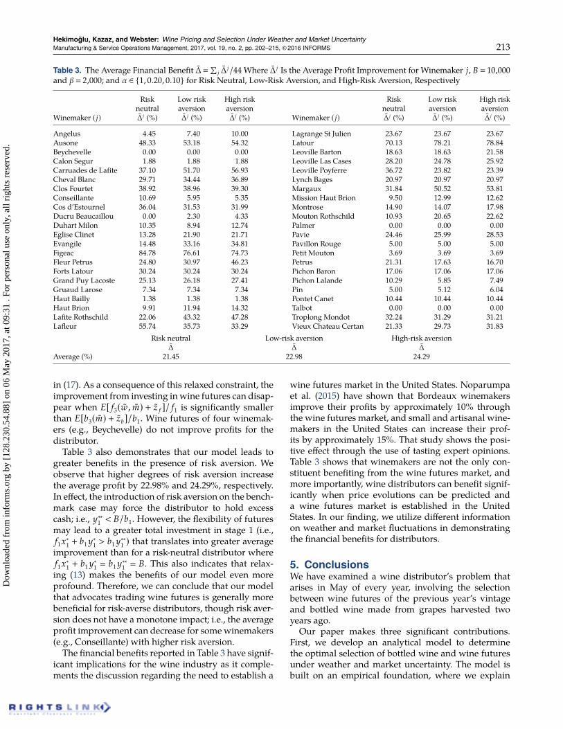
Table 3 summarizes the benefits of using our modelof investing in futures, bottles, and leaving cash underbudget (equal for each winemaker) and VaR con-straints described in (8)–(16). It presents the averagebenefit in this study as ∆ j (1/2)∑t(∆ j, t) for each of theBordeaux winemakers at different levels of risk aver-sion using tighter requirements regarding the proba-bility of loss (α).These results show that even the largest distributors,
who can be assumed to be risk neutral, would signifi-cantly benefit from investing in wine futures. The aver-age expected profit improvement from these 44 Bor-deaux wineries is 21.45%; the largest average improve-ment is 84.78% at Figeac. In our numerical analysis,we relax the assumption that wine futures and bot-tled wine have equal expected returns, as designated
Dow
nloa
ded
from
info
rms.
org
by [
128.
230.
54.8
8] o
n 06
May
201
7, a
t 09:
31 .
For
pers
onal
use
onl
y, a
ll ri
ghts
res
erve
d.
Hekimoğlu, Kazaz, and Webster: Wine Pricing and Selection Under Weather and Market UncertaintyManufacturing & Service Operations Management, 2017, vol. 19, no. 2, pp. 202–215, ©2016 INFORMS 213
Table 3. The Average Financial Benefit ∆∑
j ∆j/44 Where ∆ j Is the Average Profit Improvement for Winemaker j, B 10,000
and β 2,000; and α ∈ 1, 0.20, 0.10 for Risk Neutral, Low-Risk Aversion, and High-Risk Aversion, Respectively
Risk Low risk High risk Risk Low risk High riskneutral aversion aversion neutral aversion aversion
Winemaker ( j) ∆ j (%) ∆ j (%) ∆ j (%) Winemaker ( j) ∆ j (%) ∆ j (%) ∆ j (%)
Angelus 4.45 7.40 10.00 Lagrange St Julien 23.67 23.67 23.67Ausone 48.33 53.18 54.32 Latour 70.13 78.21 78.84Beychevelle 0.00 0.00 0.00 Leoville Barton 18.63 18.63 21.58Calon Segur 1.88 1.88 1.88 Leoville Las Cases 28.20 24.78 25.92Carruades de Lafite 37.10 51.70 56.93 Leoville Poyferre 36.72 23.82 23.39Cheval Blanc 29.71 34.44 36.89 Lynch Bages 20.97 20.97 20.97Clos Fourtet 38.92 38.96 39.30 Margaux 31.84 50.52 53.81Conseillante 10.69 5.95 5.35 Mission Haut Brion 9.50 12.99 12.62Cos d’Estournel 36.04 31.53 31.99 Montrose 14.90 14.07 17.98Ducru Beaucaillou 0.00 2.30 4.33 Mouton Rothschild 10.93 20.65 22.62Duhart Milon 10.35 8.94 12.74 Palmer 0.00 0.00 0.00Eglise Clinet 13.28 21.90 21.71 Pavie 24.46 25.99 28.53Evangile 14.48 33.16 34.81 Pavillon Rouge 5.00 5.00 5.00Figeac 84.78 76.61 74.73 Petit Mouton 3.69 3.69 3.69Fleur Petrus 24.80 30.97 46.23 Petrus 21.31 17.63 16.70Forts Latour 30.24 30.24 30.24 Pichon Baron 17.06 17.06 17.06Grand Puy Lacoste 25.13 26.18 27.41 Pichon Lalande 10.29 5.85 7.49Gruaud Larose 7.34 7.34 7.34 Pin 5.00 5.12 6.04Haut Bailly 1.38 1.38 1.38 Pontet Canet 10.44 10.44 10.44Haut Brion 9.91 11.94 14.32 Talbot 0.00 0.00 0.00Lafite Rothschild 22.06 43.32 47.28 Troplong Mondot 32.24 31.29 31.21Lafleur 55.74 35.73 33.29 Vieux Chateau Certan 21.33 29.73 31.83
Risk neutral Low-risk aversion High-risk aversion∆ ∆ ∆
Average (%) 21.45 22.98 24.29
in (17). As a consequence of this relaxed constraint, theimprovement from investing inwine futures can disap-pear when E[ f3(w , m) + z f ]/ f1 is significantly smallerthan E[b3(m) + zb]/b1. Wine futures of four winemak-ers (e.g., Beychevelle) do not improve profits for thedistributor.Table 3 also demonstrates that our model leads to
greater benefits in the presence of risk aversion. Weobserve that higher degrees of risk aversion increasethe average profit by 22.98% and 24.29%, respectively.In effect, the introduction of risk aversion on the bench-mark case may force the distributor to hold excesscash; i.e., y∗∗1 < B/b1. However, the flexibility of futuresmay lead to a greater total investment in stage 1 (i.e.,f1x∗1 + b1 y∗1 > b1 y∗∗1 ) that translates into greater averageimprovement than for a risk-neutral distributor wheref1x∗1 + b1 y∗1 b1 y∗∗1 B. This also indicates that relax-ing (13) makes the benefits of our model even moreprofound. Therefore, we can conclude that our modelthat advocates trading wine futures is generally morebeneficial for risk-averse distributors, though risk aver-sion does not have a monotone impact; i.e., the averageprofit improvement can decrease for somewinemakers(e.g., Conseillante) with higher risk aversion.The financial benefits reported in Table 3 have signif-
icant implications for the wine industry as it comple-ments the discussion regarding the need to establish a
wine futures market in the United States. Noparumpaet al. (2015) have shown that Bordeaux winemakersimprove their profits by approximately 10% throughthe wine futures market, and small and artisanal wine-makers in the United States can increase their prof-its by approximately 15%. That study shows the posi-tive effect through the use of tasting expert opinions.Table 3 shows that winemakers are not the only con-stituent benefiting from the wine futures market, andmore importantly, wine distributors can benefit signif-icantly when price evolutions can be predicted anda wine futures market is established in the UnitedStates. In our finding, we utilize different informationon weather and market fluctuations in demonstratingthe financial benefits for distributors.
5. ConclusionsWe have examined a wine distributor’s problem thatarises in May of every year, involving the selectionbetween wine futures of the previous year’s vintageand bottled wine made from grapes harvested twoyears ago.
Our paper makes three significant contributions.First, we develop an analytical model to determinethe optimal selection of bottled wine and wine futuresunder weather and market uncertainty. The model isbuilt on an empirical foundation, where we explain
Dow
nloa
ded
from
info
rms.
org
by [
128.
230.
54.8
8] o
n 06
May
201
7, a
t 09:
31 .
For
pers
onal
use
onl
y, a
ll ri
ghts
res
erve
d.
Hekimoğlu, Kazaz, and Webster: Wine Pricing and Selection Under Weather and Market Uncertainty214 Manufacturing & Service Operations Management, 2017, vol. 19, no. 2, pp. 202–215, ©2016 INFORMS
the price evolution of futures and bottles based on theweather of the upcoming vintage and changes in mar-ket conditions. The analytical model employs the fol-lowing information from the empirical analysis thatuses a comprehensive data set regarding the trade of44 most influential Bordeaux winemakers: (1) futuresprice of a vintage is negatively influenced by a warmergrowing season for the upcoming vintage, leading to alower bottle price; (2) bottle prices are not influenced byweather conditions; and (3) improving market condi-tions lead to increases in futures and bottle prices. Wedescribe the market fluctuations through the changesin the Liv-ex 100 index. In this end, the identificationof the Liv-ex 100 index as an explaining variable ofthe fluctuations in young wine prices also constitutesanother contribution to the literature.Second, we describe the optimal selection of bot-
tled wine and wine futures with a limited budgetand using a VaR measure under weather and mar-ket uncertainty. We develop the structural propertiesof the optimal decisions. We conclude that a distrib-utor should always invest in wine futures because itincreases expected profit despite being a riskier assetthan bottled wine.
Third, we demonstrate the financial benefits of usingour analytical model through the numerical illustra-tion using the same data for a large wine distributor.The hypothetical average profit improvement is signif-icant and is higher than 21% under the assumption ofequal budget allotted for each winemaker. Moreover,the hypothetical average profit improvement becomeshigher under risk aversion. Considering the wine dis-tributor with a revenue of $11.4 billion that motivatedour study, our analysis constitutes a significant eco-nomic benefit from our proposed model.
In addition to these three main findings, we alsodemonstrate the impact of variation in weather andmarket uncertainty on the distributor’s profitability.We show that higher variation in market uncertaintyincreases the expected profit; however, higher variationin weather can cause both an increase and a decreasein expected profit.
Our findings have significant implications for thewine industry, as it is likely to encourage wine distrib-utors to invest in wine futures with better informationand expectation. Moreover, it is likely to increase thetrading volume in the financial platform Liv-ex, result-ing in even better information than what our sampleprovides.
While the motivation for our empirical and analyti-cal work stems from the wine industry, our modelingperspective applies to a wide range of products andservices. In the wine industry, the weather informa-tion for the upcoming vintage can be perceived as aninformation signal that causes a reevaluation of the
quality perception in the eyes of the consumers. Vari-ous industries have similar structures. In the technol-ogy industry, for example, the information regardingthe release of new products often negatively influencesthe price of the current products. This is similar to theconsequences of observing an improved weather con-dition during the growing season of the upcoming vin-tage. What is unique in our study, however, is that theupcoming vintage’s weather information, when it is arelatively colder summer, can lead to an increase in theprice of the current vintage. This kind of price increasehas not been observed in the technology industrywhennew information regarding the upcoming products isavailable. The increased prices are only observed aftera significant amount of time, as with valuable antiques.However, the price increase in our study occurs with-out having to wait for a long period. Thus, the probleminvestigated here has unique features, as it combinessimilar characteristics of information signaling fromvarious industries for a single product and in a shortspan of time.
Our study has some limitations. Longer time seriesdata can be used to test and enrich the price evolutionof wine futures and bottled wine. Our study employsdata only from the most popular Bordeaux winemak-ers and ignores wine producers from other regions.Our work also sheds light into future research direc-tions. A longer time series data can help develop mod-els that predict the price of wine futures and bottledwine. Such prediction models can help other parties,e.g., restaurateurs and investors who engage in thetrade of wine. Our model can be expanded to con-sider other financing options such as debts and loansto increase the distributor’s budget allocation. Ourstudy, along with Noparumpa et al. (2015), points tothe potential success of a futures market in the UnitedStates. Future research needs to address regulatorypolicies and legal requirements to arrive at an economi-cally healthy futures market. Moreover, future researchcan examine the benefits of dynamically adjusting thedistributor’s budget each year in a multiperiod setting.
AcknowledgmentsThe authors are grateful to Mr. Steven R. Becker, chief finan-cial officer of Southern Wine and Spirits, for his continuedsupport; to Liv-ex for allowing us to be the first scholarsto access all of the futures and bottle trade data involvingBordeaux winemakers; and to Mr. Ben O’Donnell of WineSpectator for his comments and suggestions. The paper ben-efited from feedback from participants at presentations atArizona State University, the University of Washington, Cor-nell University, the University of Miami, Washington Univer-sity in St. Louis, and in the American Association of WineEconomists Conference at the University of Bordeaux.
ReferencesAli HH, Nauges C (2007) The pricing of experience goods: The case
of en primeur wine. Amer. J. Agricultural Econom. 89(1):91–103.
Dow
nloa
ded
from
info
rms.
org
by [
128.
230.
54.8
8] o
n 06
May
201
7, a
t 09:
31 .
For
pers
onal
use
onl
y, a
ll ri
ghts
res
erve
d.
Hekimoğlu, Kazaz, and Webster: Wine Pricing and Selection Under Weather and Market UncertaintyManufacturing & Service Operations Management, 2017, vol. 19, no. 2, pp. 202–215, ©2016 INFORMS 215
Ali HH, Lecocq S, VisserM (2008) The impact of gurus: Parker gradesand en primeur wine prices. Econom. J. 118(529):158–173.
Ashenfelter O (2008) Predicting the prices and quality of Bordeauxwines. Econom. J. 118(529):F174–F184.
Ashenfelter O, Jones GV (2013) The demand for expert opinion: Bor-deaux wine. J. Wine Econom. 8(3):285–293.
Ashenfelter O, Storchmann K (2010) Using a hedonic model ofsolar radiation to assess the economic effect of climate change:The case of Mosel Valley vineyards. Rev. Econom. Statist. 92(2):333–349.
Ashenfelter O, Ashmore D, Lalonde R (1995) Bordeaux wine vintagequality and the weather. Chance 8(4):7–13.
Boda K, Filar JA (2006) Time consistent dynamic riskmeasures.Math.Methods Oper. Res. 63(1):169–186.
Boyabatlı O (2015) Supply management in multi-product firmswith fixed proportions technology. Management Sci. 61(12):3013–3031.
Boyabatlı O, Kleindorfer P, Koontz S (2011) Integrating long-termand short-term contracting in beef supply chains. ManagementSci. 57(10):1771–1787.
Boyacı T, ÖzerÖ (2010) Information acquisition for capacity planningvia pricing and advance selling: When to stop and act. Oper. Res.58(5):1328–1349.
Burton BJ, Jacobsen JP (2001) The rate of return on investment inwine. Econom. Inquiry 39(3):337–350.
Byron RP, Ashenfelter O (1995) Predicting the quality of an unbornGrange. Econom. Record 71(1):40–53.
Cho SH, Tang CS (2013) Advance selling in a supply chain underuncertain supply and demand. Manufacturing Service Oper. Man-agement 15(2):305–319.
Devalkar S, Anupindi R, Sinha A (2015) Dynamic risk managementof commodity operations: Model and analysis. Working paper,Indian School of Business, Telangana, India.
Dimson E, Rousseau PL, Spaenjers C (2014) The price of wine.J. Financial Econom. 118(2):431–449.
Fama E, French K (1987) Commodity futures prices: Some evidenceon forecast power, premiums, and the theory of storage. J. Bus.60(1):55–73.
GemanH (2005)Commodities and Commodity Derivatives: Modeling andPricing for Agriculturals, Metals and Energy (John Wiley & Sons,New York).
Gümüş M (2014) With or without forecast sharing: Credibility andcompetition under information asymmetry. Production Oper.Management 23(10):1732–1747.
Haeger JW, Storchmann K (2006) Prices of American pinot noirwines: Climate, craftsmanship, critics. Agricultural Econom.35(1):67–78.
Jaeger E (1981) To save or savor: The rate of return to storing wine.J. Political Econom. 89(3):584–592.
Jones G, Storchmann K (2001) Wine market prices and investmentunder uncertainty: An econometric model for Bordeaux Cruclasses. Agricultural Econom. 26(2):114–33.
Jones PC, Lowe T, Traub RD, Keller G (2001) Matching supply anddemand: The value of a second chance in producing hybrid seedcorn. Manufacturing Service Oper. Management 3(2):122–137.
Kazaz B (2004) Production planning under yield and demand un-certainty. Manufacturing Service Oper. Management 6(3):209–224.
Kazaz B, Webster S (2011) The impact of yield dependent tradingcosts on pricing and production planning under supply uncer-tainty. Manufacturing Service Oper. Management 13(3):404–417.
Kazaz B, Webster S (2015) Technical note—Price-setting newsvendorproblems with uncertain supply and risk aversion. Oper. Res.63(4):807–811.
Lecocq S, Visser M (2006) Spatial variations in weather conditionsand wine prices in Bordeaux. J. Wine Econom. 1(2):114–124.
Li H, HuhWT (2011) Pricingmultiple products with themultinomiallogit and nested logit concavity: Concavity and implications.Manufacturing Service Oper. Management 13(4):549–563.
Masset P, Weisskopf JP (2010) Raise your glass: Wine investment andthe financial crisis. Working paper, Ecole hôtelière de Lausanne,Switzerland.
Noparumpa T, Kazaz B, Webster S (2015) Wine futures and advanceselling under quality uncertainty. Manufacturing Service Oper.Management 17(3):411–426.
Storchmann K (2012) Wine economics. J. Wine Econom. 7(1):1–33.Tang CS, Lim WS (2013) Advance selling in the presence of specula-
tors and forward looking consumers. Production Oper. Manage-ment 22(3):571–587.
Tomlin B, Wang Y (2008) Pricing and operational recourse in copro-duction systems. Management Sci. 54(3):522–537.
Wood D, Anderson K (2006) What determines the future value ofan icon wine? New evidence from Australia. J. Wine Econom.1(2):141–161.
Xie J, Shugan SM (2001) Electronic tickets, smart cards, and onlinepayments: When and how to advance sell. Marketing Sci. 20(3):219–243.
Yano CA, Lee H (1995) Lot sizing with random yields: A review.Oper. Res. 43(2):311–334.
Dow
nloa
ded
from
info
rms.
org
by [
128.
230.
54.8
8] o
n 06
May
201
7, a
t 09:
31 .
For
pers
onal
use
onl
y, a
ll ri
ghts
res
erve
d.