computational methods in dynamical systems and advanced ... · path following and boundary value...
TRANSCRIPT
Computational Methods in Dynamical Systemsand Advanced Examples
FisMat 2015
Obverse and reverse of the same coin [head and tails]
Jorge Galán Vioque and Emilio Freire Macías
Universidad de Sevilla
July 2015
FisMat 2015 Computational Methods in Dynamical Systems
Outline
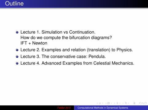
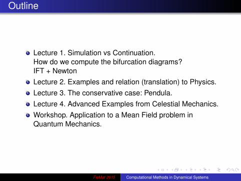
Lecture 1. Simulation vs Continuation.How do we compute the bifurcation diagrams?IFT + Newton
Lecture 2. Examples and relation (translation) to Physics.Lecture 3. The conservative case: Pendula.Lecture 4. Advanced Examples from Celestial Mechanics.Workshop. Application to a Mean Field problem inQuantum Mechanics.
FisMat 2015 Computational Methods in Dynamical Systems
Outline
Lecture 1. Simulation vs Continuation.How do we compute the bifurcation diagrams?IFT + NewtonLecture 2. Examples and relation (translation) to Physics.
Lecture 3. The conservative case: Pendula.Lecture 4. Advanced Examples from Celestial Mechanics.Workshop. Application to a Mean Field problem inQuantum Mechanics.
FisMat 2015 Computational Methods in Dynamical Systems
Outline
Lecture 1. Simulation vs Continuation.How do we compute the bifurcation diagrams?IFT + NewtonLecture 2. Examples and relation (translation) to Physics.Lecture 3. The conservative case: Pendula.
Lecture 4. Advanced Examples from Celestial Mechanics.Workshop. Application to a Mean Field problem inQuantum Mechanics.
FisMat 2015 Computational Methods in Dynamical Systems
Outline
Lecture 1. Simulation vs Continuation.How do we compute the bifurcation diagrams?IFT + NewtonLecture 2. Examples and relation (translation) to Physics.Lecture 3. The conservative case: Pendula.Lecture 4. Advanced Examples from Celestial Mechanics.
Workshop. Application to a Mean Field problem inQuantum Mechanics.
FisMat 2015 Computational Methods in Dynamical Systems
Outline
Lecture 1. Simulation vs Continuation.How do we compute the bifurcation diagrams?IFT + NewtonLecture 2. Examples and relation (translation) to Physics.Lecture 3. The conservative case: Pendula.Lecture 4. Advanced Examples from Celestial Mechanics.Workshop. Application to a Mean Field problem inQuantum Mechanics.
FisMat 2015 Computational Methods in Dynamical Systems
References
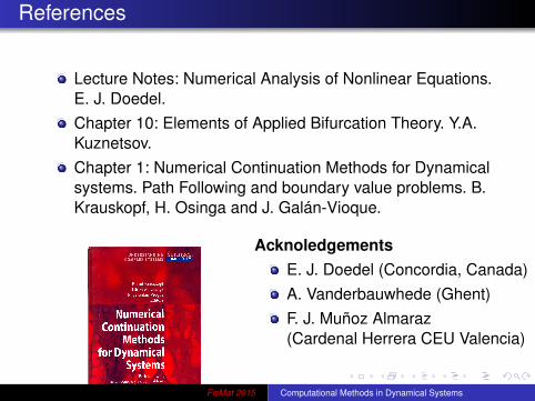
Lecture Notes: Numerical Analysis of Nonlinear Equations.E. J. Doedel.Chapter 10: Elements of Applied Bifurcation Theory. Y.A.Kuznetsov.Chapter 1: Numerical Continuation Methods for Dynamicalsystems. Path Following and boundary value problems. B.Krauskopf, H. Osinga and J. Galán-Vioque.
AcknoledgementsE. J. Doedel (Concordia, Canada)A. Vanderbauwhede (Ghent)F. J. Muñoz Almaraz(Cardenal Herrera CEU Valencia)
FisMat 2015 Computational Methods in Dynamical Systems
Excercises from Emilio’s talk
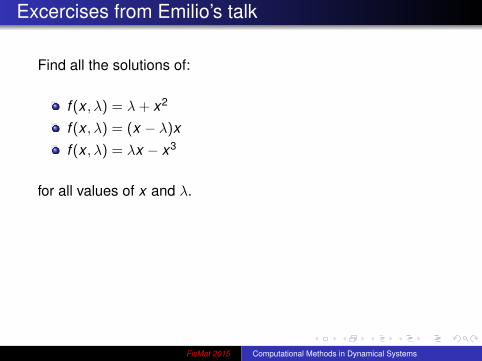
Find all the solutions of:
f (x , λ) = λ+ x2
f (x , λ) = (x − λ)xf (x , λ) = λx − x3
for all values of x and λ.
Emilio could find the solutions by hand, but
How do we get the answer with the computer?
or, how do we proceed in realistic examples?
FisMat 2015 Computational Methods in Dynamical Systems

Excercises from Emilio’s talk
Find all the solutions of:
f (x , λ) = λ+ x2
f (x , λ) = (x − λ)xf (x , λ) = λx − x3
for all values of x and λ.
Emilio could find the solutions by hand, but
How do we get the answer with the computer?
or, how do we proceed in realistic examples?
FisMat 2015 Computational Methods in Dynamical Systems
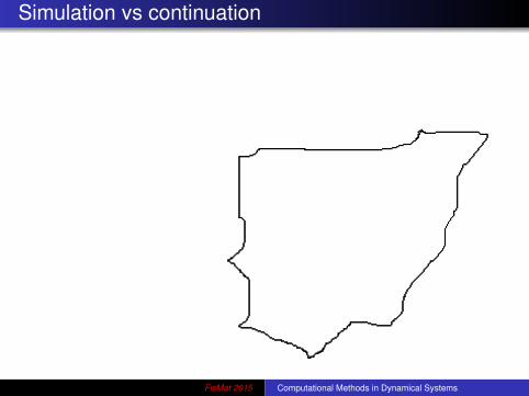
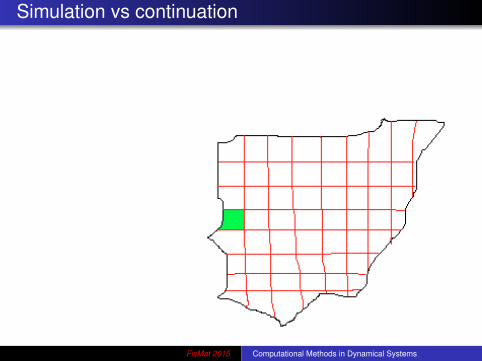
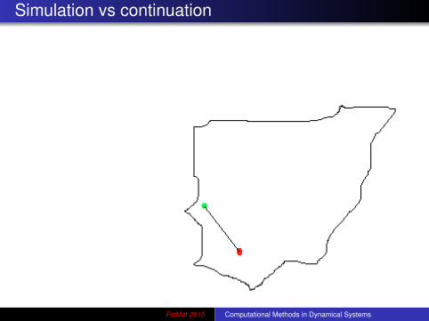
Simulation vs continuation
FisMat 2015 Computational Methods in Dynamical Systems
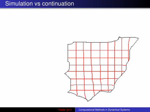
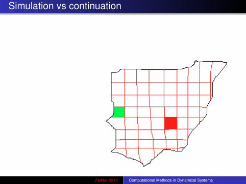
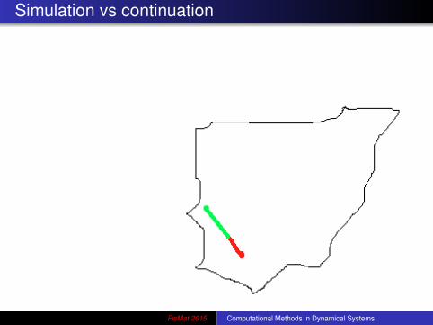
Simulation vs continuation
FisMat 2015 Computational Methods in Dynamical Systems
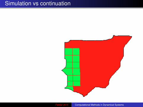
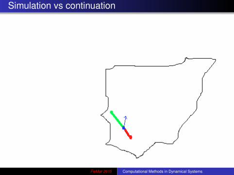
Simulation vs continuation
FisMat 2015 Computational Methods in Dynamical Systems
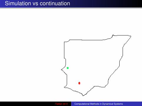
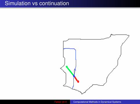
Simulation vs continuation
FisMat 2015 Computational Methods in Dynamical Systems
Simulation vs continuation
FisMat 2015 Computational Methods in Dynamical Systems
Simulation vs continuation
FisMat 2015 Computational Methods in Dynamical Systems
Simulation vs continuation
FisMat 2015 Computational Methods in Dynamical Systems
Simulation vs continuation
FisMat 2015 Computational Methods in Dynamical Systems

Simulation vs continuation
FisMat 2015 Computational Methods in Dynamical Systems
Simulation vs continuation
FisMat 2015 Computational Methods in Dynamical Systems

Simulation vs continuation
FisMat 2015 Computational Methods in Dynamical Systems
Simulation vs continuation
FisMat 2015 Computational Methods in Dynamical Systems
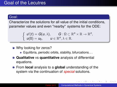
Goal of the Lecutres
Goal:Characterize the solutions for all value of the initial conditions,parameter values and even "nearby" systems for the ODE:
u′(t) = G(u, λ), G : Ω ⊂ Rn × R→ Rn,u(0) = u0, u ∈ Rn, λ ∈ R.
Why looking for zeros?Equilibria, periodic orbits, stability, bifurcations. . .
Qualitative vs quantitative analysis of differentialequations.From local analysis to a global understanding of thesystem via the continuation of special solutions.
FisMat 2015 Computational Methods in Dynamical Systems
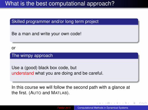
What is the best computational approach?
Skilled programmer and/or long term project
Be a man and write your own code!
or
The wimpy approach
Use a (good) black box code, butunderstand what you are doing and be careful.
In this course we will follow the second path with a glance atthe first. (AUTO and MATLAB).
FisMat 2015 Computational Methods in Dynamical Systems
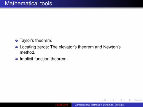
Mathematical tools
Taylor’s theorem.Locating zeros: The elevator’s theorem and Newton’smethod.Implicit function theorem.
FisMat 2015 Computational Methods in Dynamical Systems

Elevator’s theorem
This elevator takes youto the second floorwithout passingthrough the first floor.
This is imposiblesigned: Bolzano.
FisMat 2015 Computational Methods in Dynamical Systems
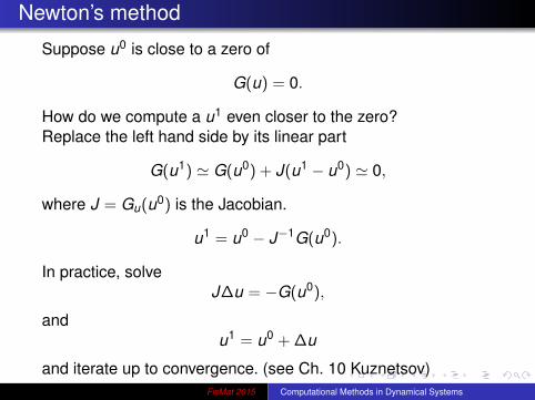
Newton’s method
Suppose u0 is close to a zero of
G(u) = 0.
How do we compute a u1 even closer to the zero?Replace the left hand side by its linear part
G(u1) ' G(u0) + J(u1 − u0) ' 0,
where J = Gu(u0) is the Jacobian.
u1 = u0 − J−1G(u0).
In practice, solveJ∆u = −G(u0),
andu1 = u0 + ∆u
and iterate up to convergence. (see Ch. 10 Kuznetsov)FisMat 2015 Computational Methods in Dynamical Systems
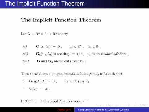
The Implicit Function Theorem
The Implicit Function Theorem
Let G : Rn × R → Rn satisfy
(i) G(u0, λ0) = 0 , u0 ∈ Rn , λ0 ∈ R .
(ii) Gu(u0, λ0) is nonsingular (i.e., u0 is an isolated solution) ,
(iii) G and Gu are smooth near u0 .
Then there exists a unique, smooth solution family u(λ) such that
G(u(λ), λ) = 0 , for all λ near λ0 ,
u(λ0) = u0 .
PROOF : See a good Analysis book · · ·
4FisMat 2015 Computational Methods in Dynamical Systems
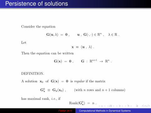
Persistence of solutions
Consider the equation
G(u, λ) = 0 , u , G(·, ·) ∈ Rn , λ ∈ R .
Letx ≡ (u , λ) .
Then the equation can be written
G(x) = 0 , G : Rn+1 → Rn .
DEFINITION.
A solution x0 of G(x) = 0 is regular if the matrix
G0x ≡ Gx(x0) , (with n rows and n+ 1 columns)
has maximal rank, i.e., ifRank(G0
x) = n .
9
FisMat 2015 Computational Methods in Dynamical Systems
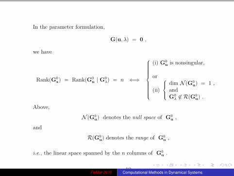
In the parameter formulation,
G(u, λ) = 0 ,
we have
Rank(G0x) = Rank(G0
u | G0λ) = n ⇐⇒
(i) G0u is nonsingular,
or
(ii)
dim N (G0u) = 1 ,
andG0λ 6∈ R(G0
u) .
Above,
N (G0u) denotes the null space of G0
u ,
and
R(G0u) denotes the range of G0
u ,
i.e., the linear space spanned by the n columns of G0u .
10FisMat 2015 Computational Methods in Dynamical Systems
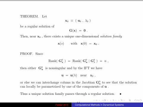
THEOREM. Letx0 ≡ ( u0 , λ0 )
be a regular solution ofG(x) = 0 .
Then, near x0 , there exists a unique one-dimensional solution family
x(s) with x(0) = x0 .
PROOF. Since
Rank( G0x ) = Rank( G0
u | G0λ ) = n ,
then either G0u is nonsingular and by the IFT we have
u = u(λ) near x0 ,
or else we can interchange colums in the Jacobian G0x to see that the solution
can locally be parametrized by one of the components of u .
Thus a unique solution family passes through a regular solution. •
11FisMat 2015 Computational Methods in Dynamical Systems
NOTE:
Such a solution family is sometimes also called a solution branch .
Case (ii) above is that of a simple fold , to be discussed later.
Thus even near a simple fold there is a unique solution family.
However, near such a fold, the family can not be parametrized by λ.
12FisMat 2015 Computational Methods in Dynamical Systems
Parameter continuation
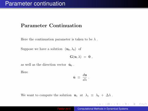
Parameter Continuation
Here the continuation parameter is taken to be λ .
Suppose we have a solution (u0, λ0) of
G(u, λ) = 0 ,
as well as the direction vector u0 .
Here
u ≡ du
dλ.
We want to compute the solution u1 at λ1 ≡ λ0 + ∆λ .
43
FisMat 2015 Computational Methods in Dynamical Systems
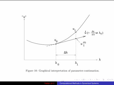
"u"
u
u
λ λλ
u 1(0)
dud λ
at λ0 )u
10
1
0
∆λ
(=
Figure 10: Graphical interpretation of parameter-continuation.
44FisMat 2015 Computational Methods in Dynamical Systems
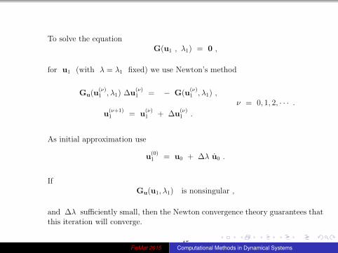
To solve the equationG(u1 , λ1) = 0 ,
for u1 (with λ = λ1 fixed) we use Newton’s method
Gu(u(ν)1 , λ1) ∆u
(ν)1 = − G(u
(ν)1 , λ1) ,
u(ν+1)1 = u
(ν)1 + ∆u
(ν)1 .
ν = 0, 1, 2, · · · .
As initial approximation use
u(0)1 = u0 + ∆λ u0 .
IfGu(u1, λ1) is nonsingular ,
and ∆λ sufficiently small, then the Newton convergence theory guarantees thatthis iteration will converge.
45FisMat 2015 Computational Methods in Dynamical Systems

After convergence, the new direction vector u1 can be computed by solving
Gu(u1, λ1) u1 = −Gλ(u1, λ1) .
This equation follows from differentiating
G(u(λ), λ) = 0 ,
with respect to λ at λ = λ1 .
NOTE:
u1 can be computed without another LU -factorization of Gu(u1, λ1) .
Thus the extra work to find u1 is negligible.
46FisMat 2015 Computational Methods in Dynamical Systems
Exercise
Excercise for Lecture 1
When will the parameter continuation fail?
FisMat 2015 Computational Methods in Dynamical Systems
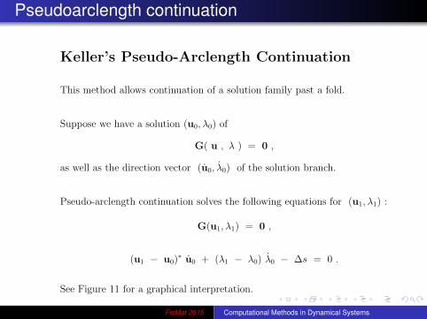
Pseudoarclength continuation
Keller’s Pseudo-Arclength Continuation
This method allows continuation of a solution family past a fold.
Suppose we have a solution (u0, λ0) of
G( u , λ ) = 0 ,
as well as the direction vector (u0, λ0) of the solution branch.
Pseudo-arclength continuation solves the following equations for (u1, λ1) :
G(u1, λ1) = 0 ,
(u1 − u0)∗ u0 + (λ1 − λ0) λ0 − ∆s = 0 .
See Figure 11 for a graphical interpretation.
51FisMat 2015 Computational Methods in Dynamical Systems
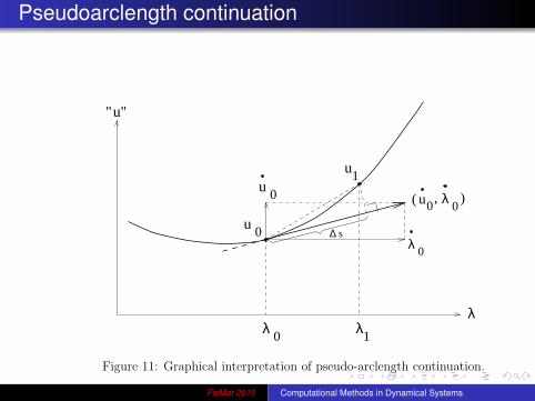
Pseudoarclength continuation
u 0
u 0 ∆ s
λ 0
"u"
λ λλ
u
10
1
u( ), λ 00
Figure 11: Graphical interpretation of pseudo-arclength continuation.
52
FisMat 2015 Computational Methods in Dynamical Systems
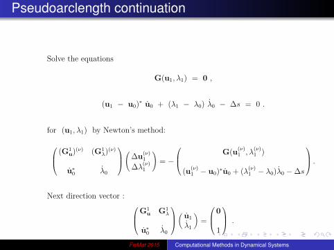
Pseudoarclength continuation
Solve the equations
G(u1, λ1) = 0 ,
(u1 − u0)∗ u0 + (λ1 − λ0) λ0 − ∆s = 0 .
for (u1, λ1) by Newton’s method:
(G1u)(ν) (G1
λ)(ν)
u∗0 λ0
(
∆u(ν)1
∆λ(ν)1
)= −
G(u(ν)1 , λ
(ν)1 )
(u(ν)1 − u0)∗u0 + (λ
(ν)1 − λ0)λ0 −∆s
.
Next direction vector :
G1u G1
λ
u∗0 λ0
(
u1
λ1
)=
0
1
.
53
FisMat 2015 Computational Methods in Dynamical Systems
Pseudoarclength continuation
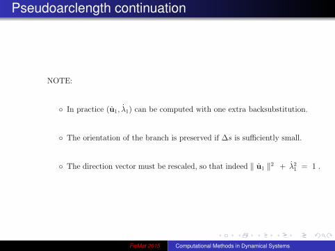
NOTE:
In practice (u1, λ1) can be computed with one extra backsubstitution.
The orientation of the branch is preserved if ∆s is sufficiently small.
The direction vector must be rescaled, so that indeed ‖ u1 ‖2 + λ21 = 1 .
54
FisMat 2015 Computational Methods in Dynamical Systems
Pseudoarclength continuation
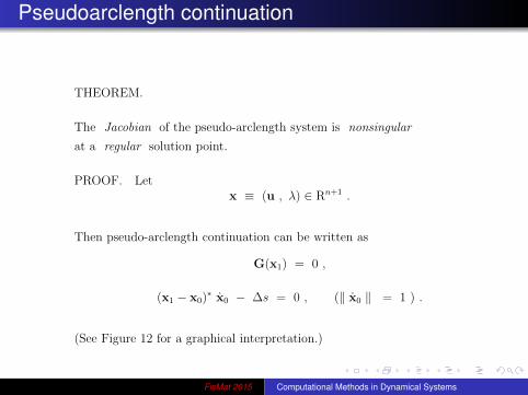
THEOREM.
The Jacobian of the pseudo-arclength system is nonsingular
at a regular solution point.
PROOF. Letx ≡ (u , λ) ∈ Rn+1 .
Then pseudo-arclength continuation can be written as
G(x1) = 0 ,
(x1 − x0)∗ x0 − ∆s = 0 , (‖ x0 ‖ = 1 ) .
(See Figure 12 for a graphical interpretation.)
55
FisMat 2015 Computational Methods in Dynamical Systems
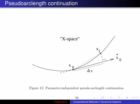
Pseudoarclength continuation
∆ s
1x
0x
"X-space"
0x
Figure 12: Parameter-independent pseudo-arclength continuation.
56FisMat 2015 Computational Methods in Dynamical Systems
Pseudoarclength continuation
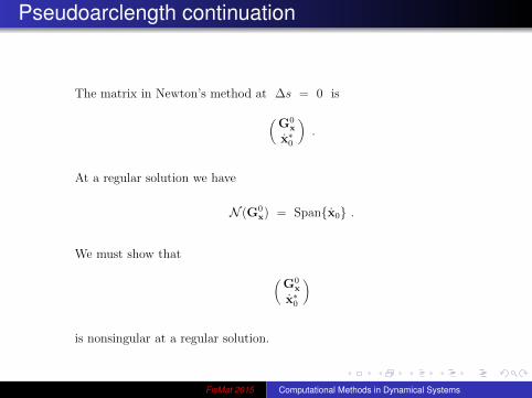
The matrix in Newton’s method at ∆s = 0 is
(G0
x
x∗0
).
At a regular solution we have
N (G0x) = Spanx0 .
We must show that
(G0
x
x∗0
)
is nonsingular at a regular solution.
57
FisMat 2015 Computational Methods in Dynamical Systems
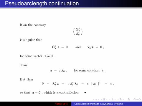
Pseudoarclength continuation
If on the contrary(
G0x
x∗0
)
is singular then
G0x z = 0 and x∗0 z = 0 ,
for some vector z 6= 0 .
Thus
z = c x0 , for some constant c .
But then0 = x∗0 z = c x∗0 x0 = c ‖ x0 ‖2 = c ,
so that z = 0 , which is a contradiction. •
58
FisMat 2015 Computational Methods in Dynamical Systems
Recall the ingredients
The building blocks for the continuation of solutions are:Newton’s method of the properly chosen function G(x).Pseudoarclength continuation.Convergence, step control and accuracy.Appropriate test function.Data handling and representation.
All these in an efficient way.Extensions:
detect and identify bifurcation pointsbranch switchinghomo- and heteroclinic orbits
FisMat 2015 Computational Methods in Dynamical Systems
Recall the ingredients
The building blocks for the continuation of solutions are:Newton’s method of the properly chosen function G(x).Pseudoarclength continuation.Convergence, step control and accuracy.Appropriate test function.Data handling and representation.
All these in an efficient way.
Extensions:detect and identify bifurcation pointsbranch switchinghomo- and heteroclinic orbits
FisMat 2015 Computational Methods in Dynamical Systems
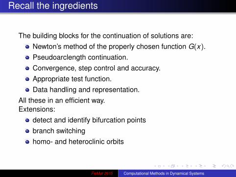
Recall the ingredients
The building blocks for the continuation of solutions are:Newton’s method of the properly chosen function G(x).Pseudoarclength continuation.Convergence, step control and accuracy.Appropriate test function.Data handling and representation.
All these in an efficient way.Extensions:
detect and identify bifurcation pointsbranch switchinghomo- and heteroclinic orbits
FisMat 2015 Computational Methods in Dynamical Systems
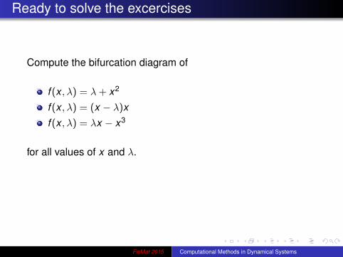
Ready to solve the excercises
Compute the bifurcation diagram of
f (x , λ) = λ+ x2
f (x , λ) = (x − λ)xf (x , λ) = λx − x3
for all values of x and λ.
Exercise Continue the perturbed pitchfork case. (add a +εterm, and continue in ε.
FisMat 2015 Computational Methods in Dynamical Systems
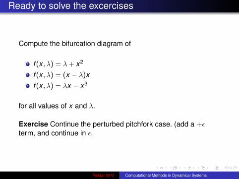
Ready to solve the excercises
Compute the bifurcation diagram of
f (x , λ) = λ+ x2
f (x , λ) = (x − λ)xf (x , λ) = λx − x3
for all values of x and λ.
Exercise Continue the perturbed pitchfork case. (add a +εterm, and continue in ε.
FisMat 2015 Computational Methods in Dynamical Systems
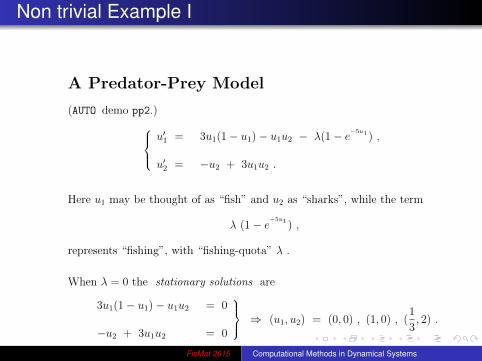
Non trivial Example I
A Predator-Prey Model
(AUTO demo pp2.)
u′1 = 3u1(1− u1)− u1u2 − λ(1− e−5u1 ) ,
u′2 = −u2 + 3u1u2 .
Here u1 may be thought of as “fish” and u2 as “sharks”, while the term
λ (1− e−5u1 ) ,
represents “fishing”, with “fishing-quota” λ .
When λ = 0 the stationary solutions are
3u1(1− u1)− u1u2 = 0
−u2 + 3u1u2 = 0
⇒ (u1, u2) = (0, 0) , (1, 0) , (
1
3, 2) .
16
FisMat 2015 Computational Methods in Dynamical Systems
The Jacobian matrix is
Gu =
(3− 6u1 − u2 − 5λe
−5u1 −u1
3u2 −1 + 3u1
)= Gu(u1, u2;λ) .
Gu(0, 0; 0) =
(3 00 −1
); eigenvalues 3,-1 (unstable) .
Gu(1, 0; 0) =
(−3 −1
0 2
); eigenvalues -3,2 (unstable) .
Gu(1
3, 2; 0) =
(−1 −1
3
6 0
); eigenvalues
(−1− µ)(−µ) + 2 = 0µ2 + µ+ 2 = 0
µ± = −1±√−72
Re(µ±) < 0 (stable) .
All three Jacobians at λ = 0 are nonsingular.
Thus, by the IFT, all three stationary points persist for (small) λ 6= 0 .
17FisMat 2015 Computational Methods in Dynamical Systems
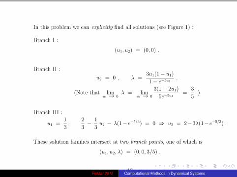
In this problem we can explicitly find all solutions (see Figure 1) :
Branch I :
(u1, u2) = (0, 0) .
Branch II :
u2 = 0 , λ =3u1(1− u1)
1− e−5u1.
(Note that limu1 → 0
λ = limu1 → 0
3(1− 2u1)
5e−5u1=
3
5.)
Branch III :
u1 =1
3,
2
3− 1
3u2 − λ(1−e−5/3) = 0 ⇒ u2 = 2−3λ(1−e−5/3) .
These solution families intersect at two branch points, one of which is
(u1, u2, λ) = (0, 0, 3/5) .
18FisMat 2015 Computational Methods in Dynamical Systems
quota0.0 0.1 0.2 0.3 0.4 0.5 0.6 0.7 0.8 0.9
sharks0.0
0.5
1.0
1.5
fish
0.00
0.25
0.50
0.75
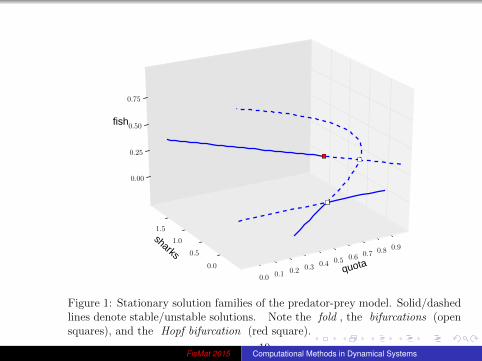
Figure 1: Stationary solution families of the predator-prey model. Solid/dashedlines denote stable/unstable solutions. Note the fold , the bifurcations (opensquares), and the Hopf bifurcation (red square).
19FisMat 2015 Computational Methods in Dynamical Systems
0.0 0.1 0.2 0.3 0.4 0.5 0.6 0.7 0.8 0.9
quota
0.0
0.2
0.4
0.6
0.8
fish
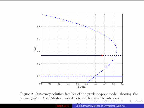
Figure 2: Stationary solution families of the predator-prey model, showing fishversus quota. Solid/dashed lines denote stable/unstable solutions.
20FisMat 2015 Computational Methods in Dynamical Systems
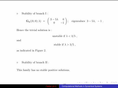
Stability of branch I :
Gu((0, 0);λ) =
(3− 5λ 0
0 −1
); eigenvalues 3− 5λ, − 1 .
Hence the trivial solution is :
unstable if λ < 3/5 ,
and
stable if λ > 3/5 ,
as indicated in Figure 2.
Stability of branch II :
This family has no stable positive solutions.
21FisMat 2015 Computational Methods in Dynamical Systems
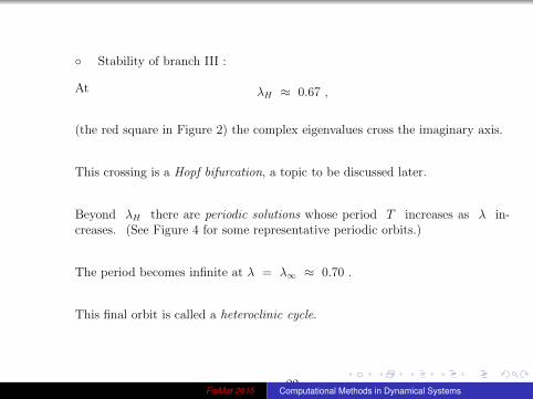
Stability of branch III :
At λH ≈ 0.67 ,
(the red square in Figure 2) the complex eigenvalues cross the imaginary axis.
This crossing is a Hopf bifurcation, a topic to be discussed later.
Beyond λH there are periodic solutions whose period T increases as λ in-creases. (See Figure 4 for some representative periodic orbits.)
The period becomes infinite at λ = λ∞ ≈ 0.70 .
This final orbit is called a heteroclinic cycle.
22FisMat 2015 Computational Methods in Dynamical Systems
0.0 0.1 0.2 0.3 0.4 0.5 0.6 0.7 0.8 0.9
quota
0.0
0.2
0.4
0.6
0.8
max
fish
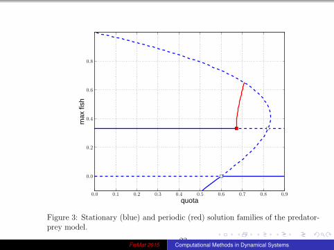
Figure 3: Stationary (blue) and periodic (red) solution families of the predator-prey model.
23FisMat 2015 Computational Methods in Dynamical Systems

0.1 0.2 0.3 0.4 0.5 0.6
fish
0.0
0.1
0.2
0.3
0.4
0.5
shar
ks
Figure 4: Some periodic solutions of the predator-prey model. The largest orbitsare very close to a heteroclinic cycle.
24FisMat 2015 Computational Methods in Dynamical Systems
From Figure 3 we can deduce the solution behavior for (slowly) increasing λ :
- Branch III is followed until λH ≈ 0.67 .
- Periodic solutions of increasing period until λ = λ∞ ≈ 0.70 .
- Collapse to trivial solution (Branch I).
EXERCISE.
Use AUTO to repeat the numerical calculations (demo pp2) .
Sketch phase plane diagrams for λ = 0, 0.5, 0.68, 0.70, 0.71 .
25FisMat 2015 Computational Methods in Dynamical Systems
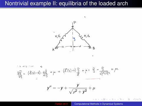
Nontrivial example II: equilibria of the loaded arch
y ′′ = −y +y√
ρ2 + y2+ µ
FisMat 2015 Computational Methods in Dynamical Systems

An example of oscillations: Hopf theorem
Analyze
du1
dt= αu1 − u2 − βu1(u2
1 + u22) (1)
du2
dt= u1 + αu2 − βu2(u2
1 + u22)
FisMat 2015 Computational Methods in Dynamical Systems
Hopf theorem
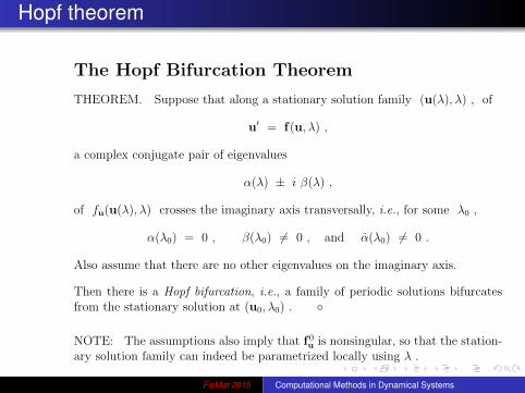
The Hopf Bifurcation Theorem
THEOREM. Suppose that along a stationary solution family (u(λ), λ) , of
u′ = f(u, λ) ,
a complex conjugate pair of eigenvalues
α(λ) ± i β(λ) ,
of fu(u(λ), λ) crosses the imaginary axis transversally, i.e., for some λ0 ,
α(λ0) = 0 , β(λ0) 6= 0 , and α(λ0) 6= 0 .
Also assume that there are no other eigenvalues on the imaginary axis.
Then there is a Hopf bifurcation, i.e., a family of periodic solutions bifurcatesfrom the stationary solution at (u0, λ0) .
NOTE: The assumptions also imply that f0u is nonsingular, so that the station-
ary solution family can indeed be parametrized locally using λ .
168FisMat 2015 Computational Methods in Dynamical Systems
Hopf theorem
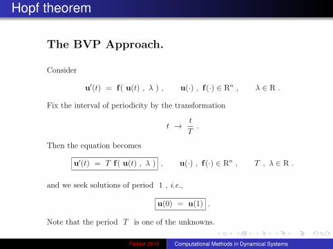
The BVP Approach.
Consider
u′(t) = f( u(t) , λ ) , u(·) , f(·) ∈ Rn , λ ∈ R .
Fix the interval of periodicity by the transformation
t → t
T.
Then the equation becomes
u′(t) = T f( u(t) , λ ) , u(·) , f(·) ∈ Rn , T , λ ∈ R .
and we seek solutions of period 1 , i.e.,
u(0) = u(1) .
Note that the period T is one of the unknowns.
190FisMat 2015 Computational Methods in Dynamical Systems
Hopf theorem
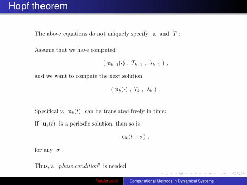
The above equations do not uniquely specify u and T :
Assume that we have computed
( uk−1(·) , Tk−1 , λk−1 ) ,
and we want to compute the next solution
( uk(·) , Tk , λk ) .
Specifically, uk(t) can be translated freely in time:
If uk(t) is a periodic solution, then so is
uk(t+ σ) ,
for any σ .
Thus, a “phase condition” is needed.
191FisMat 2015 Computational Methods in Dynamical Systems
Hopf theorem
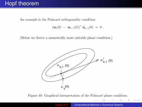
An example is the Poincare orthogonality condition
(uk(0) − uk−1(0))∗ u′k−1(0) = 0 .
(Below we derive a numerically more suitable phase condition.)
u k-1 (0)
uk-1 (0)
u (0)k
Figure 48: Graphical interpretation of the Poincare phase condition.
192FisMat 2015 Computational Methods in Dynamical Systems
Hopf theorem
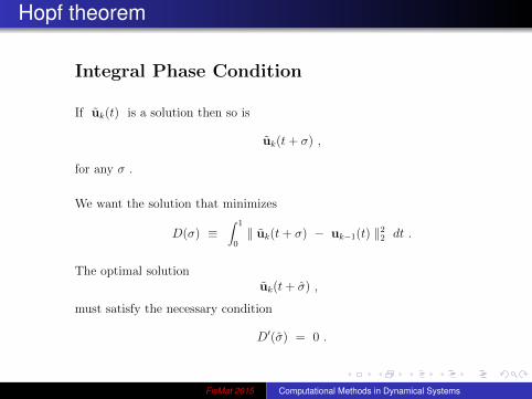
Integral Phase Condition
If uk(t) is a solution then so is
uk(t+ σ) ,
for any σ .
We want the solution that minimizes
D(σ) ≡∫ 1
0‖ uk(t+ σ) − uk−1(t) ‖2
2 dt .
The optimal solutionuk(t+ σ) ,
must satisfy the necessary condition
D′(σ) = 0 .
193FisMat 2015 Computational Methods in Dynamical Systems
Hopf theorem
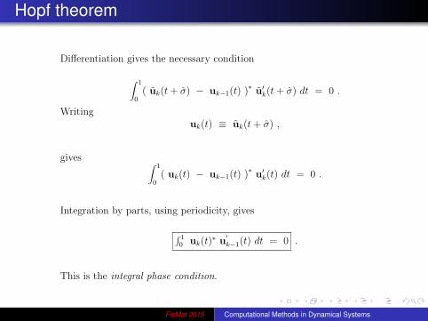
Differentiation gives the necessary condition
∫ 1
0( uk(t+ σ) − uk−1(t) )∗ u′k(t+ σ) dt = 0 .
Writinguk(t) ≡ uk(t+ σ) ,
gives ∫ 1
0( uk(t) − uk−1(t) )∗ u′k(t) dt = 0 .
Integration by parts, using periodicity, gives
∫ 10 uk(t)
∗ u′k−1(t) dt = 0 .
This is the integral phase condition.
194FisMat 2015 Computational Methods in Dynamical Systems
Hopf theorem
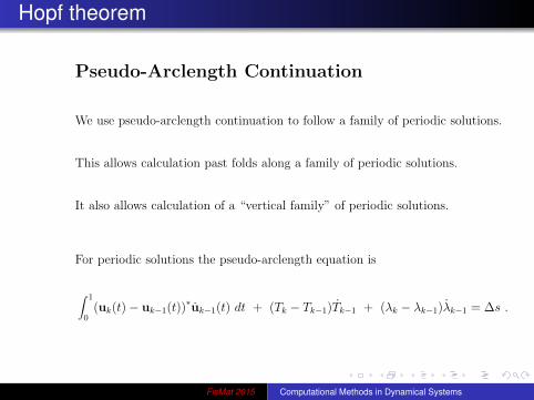
Pseudo-Arclength Continuation
We use pseudo-arclength continuation to follow a family of periodic solutions.
This allows calculation past folds along a family of periodic solutions.
It also allows calculation of a “vertical family” of periodic solutions.
For periodic solutions the pseudo-arclength equation is
∫ 1
0(uk(t)− uk−1(t))∗uk−1(t) dt + (Tk − Tk−1)Tk−1 + (λk − λk−1)λk−1 = ∆s .
195FisMat 2015 Computational Methods in Dynamical Systems
Hopf theorem
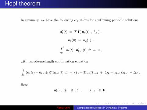
In summary, we have the following equations for continuing periodic solutions:
u′k(t) = T f( uk(t) , λk ) ,
uk(0) = uk(1) ,
∫ 1
0uk(t)
∗ u′k−1(t) dt = 0 ,
with pseudo-arclength continuation equation
∫ 1
0(uk(t)− uk−1(t))∗uk−1(t) dt + (Tk − Tk−1)Tk−1 + (λk − λk−1)λk−1 = ∆s .
Here
u(·) , f(·) ∈ Rn , λ , T ∈ R .
196FisMat 2015 Computational Methods in Dynamical Systems
Hopf theorem
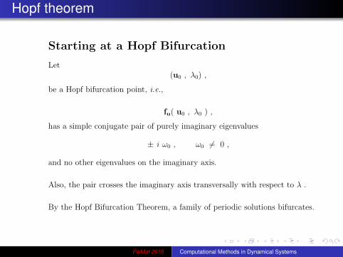
Starting at a Hopf Bifurcation
Let(u0 , λ0) ,
be a Hopf bifurcation point, i.e.,
fu( u0 , λ0 ) ,
has a simple conjugate pair of purely imaginary eigenvalues
± i ω0 , ω0 6= 0 ,
and no other eigenvalues on the imaginary axis.
Also, the pair crosses the imaginary axis transversally with respect to λ .
By the Hopf Bifurcation Theorem, a family of periodic solutions bifurcates.
197FisMat 2015 Computational Methods in Dynamical Systems
Hopf theorem
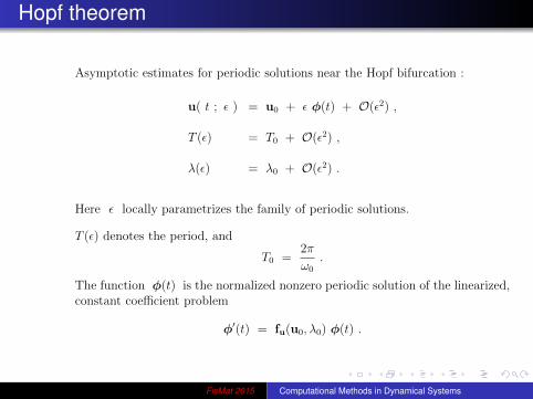
Asymptotic estimates for periodic solutions near the Hopf bifurcation :
u( t ; ε ) = u0 + ε φ(t) + O(ε2) ,
T (ε) = T0 + O(ε2) ,
λ(ε) = λ0 + O(ε2) .
Here ε locally parametrizes the family of periodic solutions.
T (ε) denotes the period, and
T0 =2π
ω0
.
The function φ(t) is the normalized nonzero periodic solution of the linearized,constant coefficient problem
φ′(t) = fu(u0, λ0) φ(t) .
198FisMat 2015 Computational Methods in Dynamical Systems
Hopf theorem
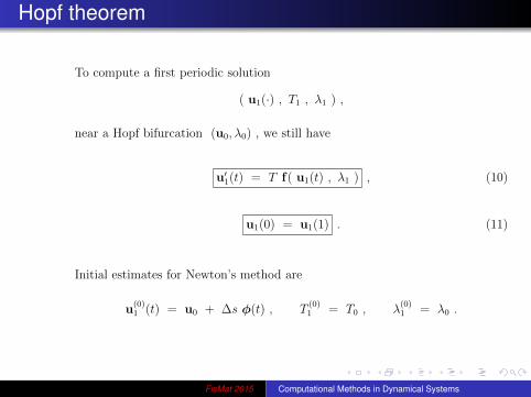
To compute a first periodic solution
( u1(·) , T1 , λ1 ) ,
near a Hopf bifurcation (u0, λ0) , we still have
u′1(t) = T f( u1(t) , λ1 ) , (10)
u1(0) = u1(1) . (11)
Initial estimates for Newton’s method are
u(0)1 (t) = u0 + ∆s φ(t) , T
(0)1 = T0 , λ
(0)1 = λ0 .
199FisMat 2015 Computational Methods in Dynamical Systems
Hopf theorem
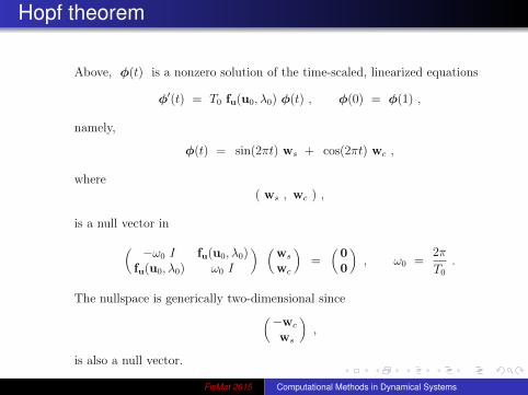
Above, φ(t) is a nonzero solution of the time-scaled, linearized equations
φ′(t) = T0 fu(u0, λ0) φ(t) , φ(0) = φ(1) ,
namely,
φ(t) = sin(2πt) ws + cos(2πt) wc ,
where( ws , wc ) ,
is a null vector in
( −ω0 I fu(u0, λ0)fu(u0, λ0) ω0 I
) (ws
wc
)=
(00
), ω0 =
2π
T0
.
The nullspace is generically two-dimensional since(−wc
ws
),
is also a null vector.
200FisMat 2015 Computational Methods in Dynamical Systems
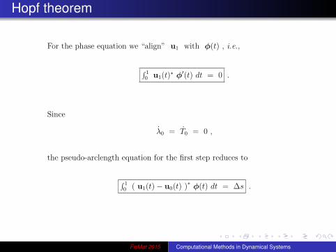
Hopf theorem
For the phase equation we “align” u1 with φ(t) , i.e.,
∫ 10 u1(t)∗ φ′(t) dt = 0 .
Since
λ0 = T0 = 0 ,
the pseudo-arclength equation for the first step reduces to
∫ 10 ( u1(t)− u0(t) )∗ φ(t) dt = ∆s .
201FisMat 2015 Computational Methods in Dynamical Systems
Numerical details
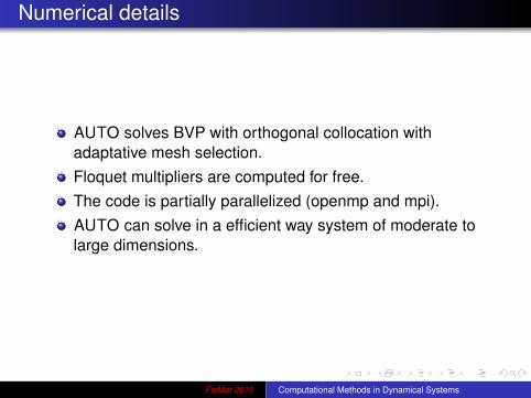
AUTO solves BVP with orthogonal collocation withadaptative mesh selection.Floquet multipliers are computed for free.The code is partially parallelized (openmp and mpi).AUTO can solve in a efficient way system of moderate tolarge dimensions.
FisMat 2015 Computational Methods in Dynamical Systems
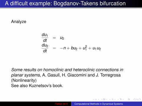
A difficult example: Bogdanov-Takens bifurcation
Analyze
du1
dt= u2
du2
dt= −n + bu2 + u2
1 + u1u2
Some results on homoclinic and heteroclinic connections inplanar systems, A. Gasull, H. Giacomini and J. Torregrosa(Nonlinearity)See also Kuznetsov’s book.
FisMat 2015 Computational Methods in Dynamical Systems
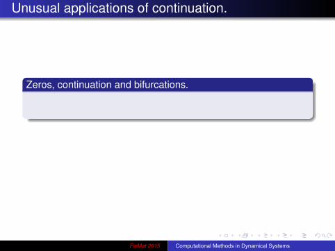
Unusual applications of continuation.
Zeros, continuation and bifurcations.
Any problem that may be formulated as G(u, λ) = 0 is suitablefor continuation.
What about computing eigenvalues?and initial value problems?
FisMat 2015 Computational Methods in Dynamical Systems
Unusual applications of continuation.
Zeros, continuation and bifurcations.Any problem that may be formulated as G(u, λ) = 0 is suitablefor continuation.
What about computing eigenvalues?and initial value problems?
FisMat 2015 Computational Methods in Dynamical Systems
Unusual applications of continuation.
Zeros, continuation and bifurcations.Any problem that may be formulated as G(u, λ) = 0 is suitablefor continuation.
What about computing eigenvalues?
and initial value problems?
FisMat 2015 Computational Methods in Dynamical Systems
Unusual applications of continuation.
Zeros, continuation and bifurcations.Any problem that may be formulated as G(u, λ) = 0 is suitablefor continuation.
What about computing eigenvalues?and initial value problems?
FisMat 2015 Computational Methods in Dynamical Systems
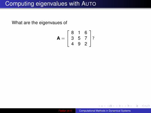
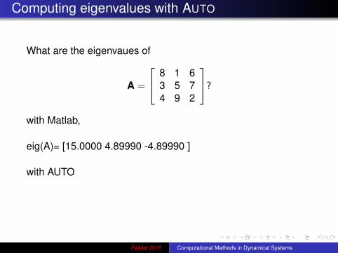
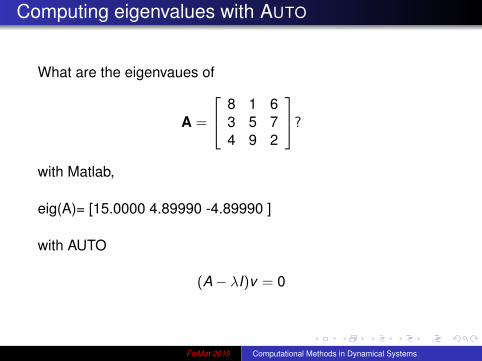
Computing eigenvalues with AUTO
What are the eigenvaues of
A =
8 1 63 5 74 9 2
?
with Matlab,
eig(A)= [15.0000 4.89990 -4.89990 ]
with AUTO
(A− λI)v = 0
FisMat 2015 Computational Methods in Dynamical Systems

Computing eigenvalues with AUTO
What are the eigenvaues of
A =
8 1 63 5 74 9 2
?
with Matlab,
eig(A)= [15.0000 4.89990 -4.89990 ]
with AUTO
(A− λI)v = 0
FisMat 2015 Computational Methods in Dynamical Systems
Computing eigenvalues with AUTO
What are the eigenvaues of
A =
8 1 63 5 74 9 2
?
with Matlab,
eig(A)= [15.0000 4.89990 -4.89990 ]
with AUTO
(A− λI)v = 0
FisMat 2015 Computational Methods in Dynamical Systems
Computing eigenvalues with AUTO
What are the eigenvaues of
A =
8 1 63 5 74 9 2
?
with Matlab,
eig(A)= [15.0000 4.89990 -4.89990 ]
with AUTO
(A− λI)v = 0
FisMat 2015 Computational Methods in Dynamical Systems
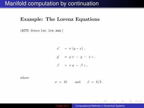
Manifold computation by continuation
Example: The Lorenz Equations
(AUTO demos lor, lrz, man.)
x′ = σ (y − x) ,
y′ = ρ x − y − x z ,
z′ = x y − β z ,
whereσ = 10 and β = 8/3 .
267FisMat 2015 Computational Methods in Dynamical Systems
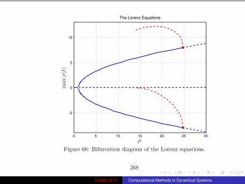
Figure 68: Bifurcation diagram of the Lorenz equations.
268
FisMat 2015 Computational Methods in Dynamical Systems

NOTE:
The zero solution is unstable for ρ > 1 .
Two nonzero stationary solutions bifurcate at ρ = 1 .
The nonzero stationary solutions become unstable for ρ > ρH .
At ρH ( ρH ≈ 24.7 ) there are Hopf bifurcations.
Unstable periodic solutions emanate from each Hopf bifurcation.
These families end in homoclinic orbits (infinite period) at ρ ≈ 13.9 .
For ρ > ρH there is the famous Lorenz attractor.
269
FisMat 2015 Computational Methods in Dynamical Systems
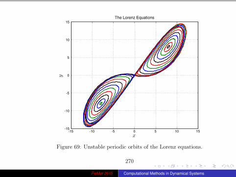
Figure 69: Unstable periodic orbits of the Lorenz equations.
270
FisMat 2015 Computational Methods in Dynamical Systems
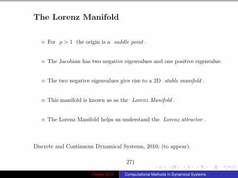
The Lorenz Manifold
For ρ > 1 the origin is a saddle point .
The Jacobian has two negative eigenvalues and one positive eigenvalue.
The two negative eigenvalues give rise to a 2D stable manifold .
This manifold is known as as the Lorenz Manifold .
The Lorenz Manifold helps us understand the Lorenz attractor .
Discrete and Continuous Dynamical Systems, 2010; (to appear).
271
FisMat 2015 Computational Methods in Dynamical Systems
-30 -20 -10 0 10 20 30X
0
25
50
75
100
125
150
175
Z
The Lorenz Equations: rho = 60
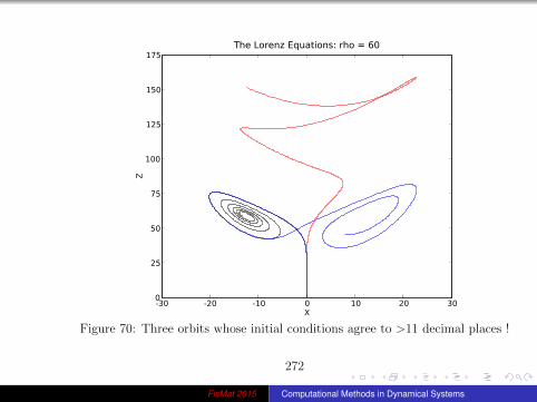
Figure 70: Three orbits whose initial conditions agree to >11 decimal places !
272
FisMat 2015 Computational Methods in Dynamical Systems
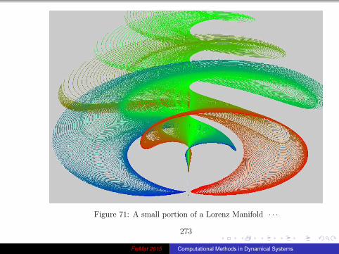
Figure 71: A small portion of a Lorenz Manifold · · ·
273
FisMat 2015 Computational Methods in Dynamical Systems
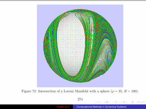
Figure 72: Intersection of a Lorenz Manifold with a sphere (ρ = 35, R = 100).
274
FisMat 2015 Computational Methods in Dynamical Systems

Figure 73: Intersection of a Lorenz Manifold with a sphere (ρ = 35, R = 100).
275
FisMat 2015 Computational Methods in Dynamical Systems
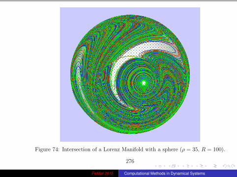
Figure 74: Intersection of a Lorenz Manifold with a sphere (ρ = 35, R = 100).
276
FisMat 2015 Computational Methods in Dynamical Systems
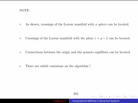
NOTE:
As shown, crossings of the Lorenz manifold with a sphere can be located.
Crossings of the Lorenz manifold with the plane z = ρ− 1 can be located.
Connections between the origin and the nonzero equilibria can be located.
There are subtle variations on the algorithm !
282
FisMat 2015 Computational Methods in Dynamical Systems

-300 -200 -100 0 100 200 300X
-100
-50
0
50
100
Y
Lorenz Section: rho= 60
Figure 75: Crossings of the Lorenz Manifold with the plane z = ρ− 1283
FisMat 2015 Computational Methods in Dynamical Systems