design of energy-efficient approximate arithmetic circuits …

DESIGN OF ENERGY-EFFICIENT APPROXIMATE ARITHMETIC CIRCUITS

A Thesis

by

BOTANG SHAO

Submitted to the Office of Graduate and Professional Studies of

Texas A&M University

in partial fulfillment of the requirements for the degree of

MASTER OF SCIENCE

Chair of Committee, Peng Li

Committee Members, Seong Gwan Choi

Rabi N. Mahapatra

Head of Department, Chanan Singh

August 2014

Major Subject: Computer Engineering

Copyright 2014 Botang Shao

ii

ABSTRACT

Energy consumption has become one of the most critical design challenges in

integrated circuit design. Arithmetic computing circuits, in particular array-based

arithmetic computing circuits such as adders, multipliers, squarers, have been widely

used. In many cases, array-based arithmetic computing circuits consume a significant

amount of energy in a chip design. Hence, reduction of energy consumption of array-

based arithmetic computing circuits is an important design consideration. To this end,

designing low-power arithmetic circuits by intelligently trading off processing precision

for energy saving in error-resilient applications such as DSP, machine learning and

neuromorphic circuits provides a promising solution to the energy dissipation challenge

of such systems.

To solve the chip’s energy problem, especially for those applications with

inherent error resilience, array-based approximate arithmetic computing (AAAC)

circuits that produce errors while having improved energy efficiency have been

proposed. Specifically, a number of approximate adders, multipliers and squarers have

been presented in the literature. However, the chief limitation of these designs is their

un-optimized processing accuracy, which is largely due to the current lack of systemic

guidance for array-based AAAC circuit design pertaining to optimal tradeoffs between

error, energy and area overhead.

Therefore, in this research, our first contribution is to propose a general model

for approximate array-based approximate arithmetic computing to guide the

iii

minimization of processing error. As part of this model, the Error Compensation Unit

(ECU) is identified as a key building block for a wide range of AAAC circuits. We

develop theoretical analysis geared towards addressing two critical design problems of

the ECU, namely, determination of optimal error compensation values and identification

of the optimal error compensation scheme. We demonstrate how this general AAAC

model can be leveraged to derive practical design insights that may lead to optimal

tradeoffs between accuracy, energy dissipation and area overhead. To further minimize

energy consumption, delay and area of AAAC circuits, we perform ECU logic

simplification by introducing don't cares.

By applying the proposed model, we propose an approximate 16x16 fixed-width

Booth multiplier that consumes 44.85% and 28.33% less energy and area compared with

theoretically the most accurate fixed-width Booth multiplier when implemented using a

90nm CMOS standard cell library. Furthermore, it reduces average error, max error and

mean square error by 11.11%, 28.11% and 25.00%, respectively, when compared with

the best reported approximate Booth multiplier and outperforms the best reported

approximate design significantly by 19.10% in terms of the energy-delay-mean square

error product (𝐸𝐷𝐸𝑚𝑠).

Using the same approach, significant energy consumption, area and error

reduction is achieved for a squarer unit, with more than 20.00% 𝐸𝐷𝐸𝑚𝑠 reduction over

existing fixed-width squarer designs. To further reduce error and cost by utilizing extra

signatures and don't cares, we demonstrate a 16-bit fixed-width squarer that improves the

energy-delay-max error (𝐸𝐷𝐸𝑚𝑎𝑥) by 15.81%.

iv

DEDICATION

To my parents and twin brother

v

ACKNOWLEDGEMENTS

It would not have been possible for me to finish such a project that involves a

large number of principles, experiments and various methods without the help and

encouragement of many people.

First and most importantly, I would like to thank my advisor Prof. Peng Li, who

supported me for the project and gave me so much guidance and help with great patience

during the last fifteen months. Whenever I had problems on the project, he would give

me suggestions by meetings or sending emails, even when it was late at night. Prof. Li

had such a significant impact on me with his hard work, dedication to perfection and

excellence and enthusiasm for research, which will also impact significantly on my

future work in industry.

Secondly, many thanks to Prof. Mahapatra and Prof. Choi who spent time

attending my defense and helped improve my research by giving me many valuable

suggestions on the project.

I would also like to remember and thank for my lab partners, Qian Wang,

Honghuang Lin, Jingwei Xu, Ahmad Bashaireh and Yongtae Kim who gave me

suggestions and much help for the usage of tools and software.

Last but not least, I would like to express my sincere acknowledgement to my

parents and twin brother. They kept encouraging me when I was in trouble and

especially, I got much encouragement from my twin brother who is now a PhD student

in one of the best medical universities in China and is working so hard on his research.

vi

TABLE OF CONTENTS

Page

ABSTRACT .......................................................................................................................ii

DEDICATION .................................................................................................................. iv

ACKNOWLEDGEMENTS ............................................................................................... v

TABLE OF CONTENTS .................................................................................................. vi

LIST OF FIGURES ........................................................................................................ viii

LIST OF TABLES ............................................................................................................. x

1. INTRODUCTION .......................................................................................................... 1

1.1 Motivation ................................................................................................................ 1

1.2 Previous work ........................................................................................................... 3

1.2.1 Approximate multipliers .................................................................................... 3

1.2.2 Approximate squarers ........................................................................................ 4

2. ARRAY-BASED APPROXIMATE ARITHMETIC COMPUTING (AAAC)

MODEL .............................................................................................................................. 5

2.1 Error Metrics ............................................................................................................ 6

2.2 Model of Error Compensation Unit (ECU) .............................................................. 7

2.3 Ideal Error Compensation & ECU Design ............................................................... 9

2.4 Further Reduction of Error and Cost ...................................................................... 13

2.5 Practical ECU Design Guidance ............................................................................ 16

3. PROPOSED MULTIPLIER DESIGN ......................................................................... 18

3.1 Fundamentals of Booth Multipliers........................................................................ 18

3.2 The Basic Idea ........................................................................................................ 19

3.3 Design of Error Compensation Unit....................................................................... 24

3.4 The Complete Fixed-Width Multiplier .................................................................. 28

3.5 Proposed Full-Width Booth Multiplier .................................................................. 29

4. PROPOSED SQUARER DESIGN .............................................................................. 31

4.1 The Basic Squarer Design ...................................................................................... 31

4.2 Further Error and Cost Reduction for Fixed-Width Squarers ................................ 33

5. COMPRESSORS FOR MULTIPLIER AND SQUARER DESIGN ........................... 36

vii

5.1 2:2 Compressors ..................................................................................................... 37

5.2 3:2 Compressors ..................................................................................................... 38

5.3 4:2 (5:3) Compressors ............................................................................................ 39

5.4 Using Compressors to Compress Array-Based Partial Product Table ................... 39

6. EXPERIMENTAL RESULTS ..................................................................................... 42

6.1 Comparison of Different Multipliers ..................................................................... 43

6.2 Accuracy Analysis for the Approximate Multipliers ............................................. 45

6.2.1 Fixed-Width Booth Multipliers ....................................................................... 45

6.2.2 Full-Width Booth Multipliers .......................................................................... 50

6.3 Comparison of Different Squarers ......................................................................... 54

6.4 Accuracy Analysis for Squarers ............................................................................. 56

6.4.1 Fixed-Width Squarers ...................................................................................... 56

6.4.2 Full-Width Squarers ........................................................................................ 60

6.5 Further Reduction of Error and Cost For the 16-bit Fixed-Width Squarer ............ 63

7. CONCLUSION ............................................................................................................ 66

REFERENCES ................................................................................................................. 67

viii

LIST OF FIGURES

Page

Figure 1. Arithmetic computing unit models: (a) Error-Free Computing Unit (EFCU)

model (large energy consumption, area and delay), (b) Proposed AAAC

model (small energy consumption, area and delay). .......................................... 5

Figure 2. ECU model: (a) Signature generator, (b) Fixed compensation per input

group. .................................................................................................................. 8

Figure 3. Classification of the inputs based on the signatures. .......................................... 9

Figure 4. A 4-group example for Theorem 4. .................................................................. 12

Figure 5. Error-Free Booth multiplier blocks. .................................................................. 18

Figure 6. Schematics of Radix-4 Booth encoding block: (a) Schematic of , 𝑠𝑖, 𝑑𝑖

generation, (b) Schematic of 𝑛𝑖 generation, (c) Schematic of 𝑧𝑖 generation,

(d) Schematic of 𝑐𝑖 generation. ......................................................................... 20

Figure 7. Schematic of the selection block. ..................................................................... 21

Figure 8. Partial product diagram for fixed-width 16x16 bits Booth multipliers

(n=16). .............................................................................................................. 21

Figure 9. Blocks and schematics of Signature Generator. ............................................... 27

Figure 10. Blocks of sorting network. .............................................................................. 27

Figure 11. Squaring diagram for 16-bit fixed-width squarers. ......................................... 31

Figure 12. Complete designs blocks: (a) the proposed multipliers, (b) the proposed

squarers. ............................................................................................................ 37

Figure 13. Block diagram of a 2:2 compressor. ............................................................... 38

Figure 14. Blocks of a 3:2 compressor. ............................................................................ 38

Figure 15. Using 2:2 and 3:2 compressors to compress an array-based partial product

table. .................................................................................................................. 40

Figure 16. 𝐸𝐷𝐸𝑚𝑠 reduction of the proposed 16x16 bits fixed-width multipliers over

DTM, PTM, PEBM and ZSM. ......................................................................... 44

ix

Figure 17. Error reduction of the proposed 8x8 fixed-width Booth multiplier over

DTM, PEBM, ZSM. ......................................................................................... 46


DTM, PEBM, ZSM. ......................................................................................... 47


DTM, PEBM, ZSM. ......................................................................................... 48


DTM, PEBM, ZSM. ......................................................................................... 49

Figure 21. Error reduction of the proposed 8x8 full-width Booth multiplier over

PEBM, ZSM. .................................................................................................... 50


PEBM, ZSM. .................................................................................................... 51


PEBM, ZSM. .................................................................................................... 52


PEBM, ZSM. .................................................................................................... 53

Figure 25.𝐸𝐷𝐸𝑚𝑠 reduction of the proposed 16-bit fixed-width squarer over DTS,

PTS, CCS and VCS. ......................................................................................... 55

Figure 26. Error reduction of the proposed 8-bit fixed-width squarer over DTS, CCS,

VCS................................................................................................................... 57

Figure 27. Error reduction of the proposed 12-bit fixed-width squarer over DTS,

CCS, VCS. ........................................................................................................ 58


CCS, VCS. ........................................................................................................ 59

Figure 29. Error reduction of the proposed 8-bit full-width squarer over CCS, VCS. .... 60

Figure 30. Error reduction of the proposed 12-bit full-width squarer over CCS, VCS. .. 61

Figure 31. Error reduction of the proposed 16-bit full-width squarer over CCS, VCS. .. 62

Figure 32. Comparison of 𝐸𝐷𝐸𝑚𝑎𝑥 of 16-bit fixed-width squarers with extra input

signatures. ......................................................................................................... 64

x

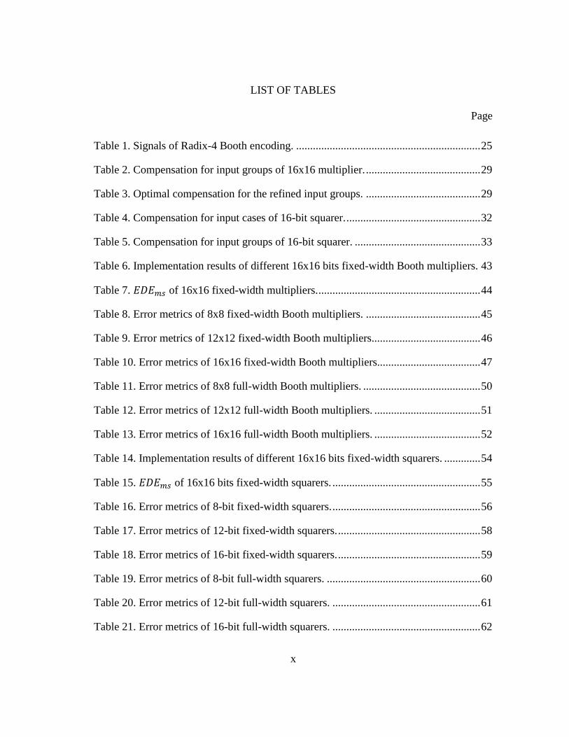
LIST OF TABLES

Page

Table 1. Signals of Radix-4 Booth encoding. .................................................................. 25

Table 2. Compensation for input groups of 16x16 multiplier. ......................................... 29

Table 3. Optimal compensation for the refined input groups. ......................................... 29

Table 4. Compensation for input cases of 16-bit squarer. ................................................ 32

Table 5. Compensation for input groups of 16-bit squarer. ............................................. 33

Table 6. Implementation results of different 16x16 bits fixed-width Booth multipliers. 43

Table 7. 𝐸𝐷𝐸𝑚𝑠 of 16x16 fixed-width multipliers. .......................................................... 44

Table 8. Error metrics of 8x8 fixed-width Booth multipliers. ......................................... 45

Table 9. Error metrics of 12x12 fixed-width Booth multipliers....................................... 46

Table 10. Error metrics of 16x16 fixed-width Booth multipliers..................................... 47

Table 11. Error metrics of 8x8 full-width Booth multipliers. .......................................... 50

Table 12. Error metrics of 12x12 full-width Booth multipliers. ...................................... 51

Table 13. Error metrics of 16x16 full-width Booth multipliers. ...................................... 52

Table 14. Implementation results of different 16x16 bits fixed-width squarers. ............. 54

Table 15. 𝐸𝐷𝐸𝑚𝑠 of 16x16 bits fixed-width squarers. ..................................................... 55

Table 16. Error metrics of 8-bit fixed-width squarers. ..................................................... 56

Table 17. Error metrics of 12-bit fixed-width squarers. ................................................... 58

Table 18. Error metrics of 16-bit fixed-width squarers. ................................................... 59

Table 19. Error metrics of 8-bit full-width squarers. ....................................................... 60

Table 20. Error metrics of 12-bit full-width squarers. ..................................................... 61

Table 21. Error metrics of 16-bit full-width squarers. ..................................................... 62

xi

Table 22. Optimal extra signatures for given number of extra signatures. ...................... 63

Table 23. 𝐸𝐷𝐸𝑚𝑎𝑥 of 16-bit fixed-width squarers with extra signatures. ........................ 64

1

1. INTRODUCTION

1.1 Motivation

As the CMOS technology and VLSI design complexity scale, delivering desired

functionalities while managing chip power consumption has become a first-class design

challenge. To remedy this grand energy-efficiency challenge, approximate arithmetic

circuits, in particular array-based approximate arithmetic computing (AAAC) circuits,

have been introduced as a promising solution to applications with inherent error

resilience including media processing, machine learning and neuromorphic systems.

AAAC may allow one to trade off accuracy for significant reduction of energy

consumption for such error tolerant applications.

To this end, approximate multipliers and squarers have been a focus of a great

deal of past and ongoing work. Two types of approximate multipliers exist: approximate

AND-array multipliers, which utilize AND gates for partial product generation [1]-[2]

and approximate Booth multipliers [3]-[8], which use the modified Booth algorithm to

reduce the number of partial products. For squarer units, a series of approximate squarers

have been proposed [9]-[11].

While a diverse set of array-based approximate arithmetic unit designs exist,

what is currently lacking is systemic design guidance that allows one to optimally

tradeoff between error, area and energy. While the area and energy of a given design can

often be easily reasoned or estimated, getting insights on error and thereby providing a

2

basis for optimally trading off between error, area and energy consumption appears to be

challenging and not well understood.

To this end, the main contributions of this research are twofold. First, a general

AAAC model is proposed for reasoning about different ways of controlling

approximation errors and present optimal error compensation schemes under ideal

design scenarios. The proposed model is general in the sense that it captures the key

design structure that is common to a major class of array-based approximate arithmetic

units (e.g., multipliers, squarers, dividers, adders/subtractors and logarithmic function

units). The proposed model offers critical insights of optimized error compensation

schemes and the corresponding signatures generation logic that is the key to error

compensation.

Second, as two specific applications, by leveraging the design insights obtained

from the proposed model, this thesis presents a new approximate Booth multiplier and

squarer design that achieve noticeable reduction of error compared with existing designs

while maintaining significant benefits in terms of delay, area and energy consumption

due to the approximate nature of computation.

The proposed approximate 16-bit fixed-width Booth multiplier consumes 44.85%

and 28.33% less energy and area compared with theoretically the most accurate fixed-

width Booth multiplier. Furthermore, it reduces average error, max error and mean

square error by 11.11%, 28.11% and 25.00%, respectively, when compared with the best

reported approximate Booth multiplier and outperforms the best reported approximate

design significantly by 19.10% in terms of the energy-delay-mean square error product

3

(𝐸𝐷𝐸𝑚𝑠). For the proposed approximate 16-bit fixed-width squarer, a 18.18%, 21.67%

and 31.25% reduction is achieved on average error, max error and mean square error,

respectively. Furthermore, 𝐸𝐷𝐸𝑚𝑠 is improved by more than 20.00%, when compared

with existing designs. By utilizing extra signatures and don’t cares, the energy-delay-

max error product (𝐸𝐷𝐸𝑚𝑎𝑥) is further reduced by 15.81% for the proposed 16-bit fixed-

width squarer. Additionally, when operated in the full-width mode, the proposed

multiplier and squarer have an even greater improvement of accuracy.

1.2 Previous work

1.2.1 Approximate multipliers

As mentioned in Sub-section 1.1, there are mainly two types of approximate

multipliers existing: approximate AND-array multipliers, which utilize AND gates for

partial products generation and approximate Booth multipliers, which use the modified

Booth algorithm to reduce the number of partial products. Constant correction [1] and

variable correction [2] schemes are proposed for approximate AND-array multipliers.

Constant correction scheme suggests adding one constant to compensate for the

truncated error and variable correction multipliers add some signals in the partial product

table to make compensation.

However, since Booth multipliers are much more efficient than AND-array

multipliers, approximate Booth multipliers have been intensively investigated [3]-[8]. In

particular, statistical linear regression analysis [3], estimation threshold calculation [4]

and self-compensation approach [5] have been utilized to compensate the truncation

error. Accuracy is increased by using certain outputs from Booth encoders [6] [7]. To

4

decrease energy consumption, a probabilistic estimation bias (PEB) scheme [8] is

presented.

1.2.2 Approximate squarers

A series of approximate squarers have been proposed [9]-[11]. For instance, the

designs of [9] and [10] compensate truncation error by utilizing constant and variable

correction scheme, respectively. A LUT-based squarer [11] is proposed by employing a

hybrid LUT-based structure.

5

2. ARRAY-BASED APPROXIMATE ARITHMETIC COMPUTING (AAAC) MODEL

Fig. 1 contrasts an Error-Free Computing Unit (EFCU) with n-bit inputs and an

m-bit output (a) with its approximate counterpart modeled using the proposed AAAC

model (b). The AAAC model consists of three units: Low-Precision Computing Unit

(LPCU), Error Compensation Unit (ECU) and Combine Unit (CU).

(a)

(b)

Figure 1. Arithmetic computing unit models: (a) Error-Free Computing Unit

(EFCU) model (large energy consumption, area and delay), (b) Proposed AAAC

model (small energy consumption, area and delay).

6

The LPCU in the AAAC circuit produces a low-precision approximate output,

for example, based upon truncation or a fraction of the input bits, with lowered energy,

delay and/or area overheads compared with the error-free EFCU.

To reduce the error produced by the LPCU, a low-cost ECU may be included for

error comparison. Finally, the CU combines the error compensation produced by the

ECU with the result outputted by the LPCU, generating the final output of the AAAC

unit with reduced approximate error.

The generality of the AAAC model lies in the fact it reflects the key computing

principles behind a wide range of array-based arithmetic units, for example, approximate

adders [12]-[14], approximate multipliers [1]-[8] and approximate squarers [9]-[11]. For

instance, many approximate adders employ carry prediction from low input bits, which

can be thought as a particular way of implementing the ECU. Similarly, error

compensation is a common scheme in approximate multipliers and squarers.

Clearly, the key AAAC design problem is to develop an efficient LPCU and, in

particular, an ECU so as to significantly reduce energy, delay and/or area overhead while

achieving a low degree of approximation error. While the area and energy of a given

design can often be easily reasoned or estimated, the key challenge is to develop insights

on error or error distribution so as to optimize the error compensation scheme, which is

focused on in the following sections.

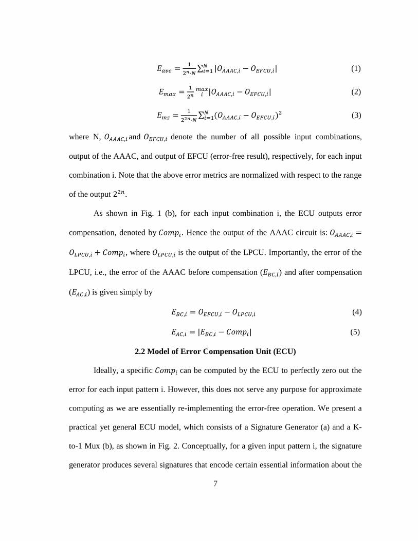
2.1 Error Metrics

This research evaluates a given AAAC design with n-bit inputs by defining

average error 𝐸𝑎𝑣𝑒, maximum error 𝐸𝑚𝑎𝑥 and mean square error 𝐸𝑚𝑠, respectively as

7

𝐸𝑎𝑣𝑒 =1

2𝑛·𝑁∑ |𝑂𝐴𝐴𝐴𝐶,𝑖 − 𝑂𝐸𝐹𝐶𝑈,𝑖|

𝑁𝑖=1 (1)

𝐸𝑚𝑎𝑥 =1

2𝑛 |𝑂𝐴𝐴𝐴𝐶,𝑖 − 𝑂𝐸𝐹𝐶𝑈,𝑖|𝑖 𝑚𝑎𝑥 (2)

𝐸𝑚𝑠 =1

22𝑛·𝑁∑ (𝑂𝐴𝐴𝐴𝐶,𝑖 − 𝑂𝐸𝐹𝐶𝑈,𝑖)²𝑁

𝑖=1 (3)

where N, 𝑂𝐴𝐴𝐴𝐶,𝑖 and 𝑂𝐸𝐹𝐶𝑈,𝑖 denote the number of all possible input combinations,

output of the AAAC, and output of EFCU (error-free result), respectively, for each input

combination i. Note that the above error metrics are normalized with respect to the range

of the output 22𝑛.

As shown in Fig. 1 (b), for each input combination i, the ECU outputs error

compensation, denoted by 𝐶𝑜𝑚𝑝𝑖. Hence the output of the AAAC circuit is: 𝑂𝐴𝐴𝐴𝐶,𝑖 =

𝑂𝐿𝑃𝐶𝑈,𝑖 + 𝐶𝑜𝑚𝑝𝑖, where 𝑂𝐿𝑃𝐶𝑈,𝑖 is the output of the LPCU. Importantly, the error of the

LPCU, i.e., the error of the AAAC before compensation (𝐸𝐵𝐶,𝑖) and after compensation

(𝐸𝐴𝐶,𝑖) is given simply by

𝐸𝐵𝐶,𝑖 = 𝑂𝐸𝐹𝐶𝑈,𝑖 − 𝑂𝐿𝑃𝐶𝑈,𝑖 (4)

𝐸𝐴𝐶,𝑖 = |𝐸𝐵𝐶,𝑖 − 𝐶𝑜𝑚𝑝𝑖| (5)

2.2 Model of Error Compensation Unit (ECU)

Ideally, a specific 𝐶𝑜𝑚𝑝𝑖 can be computed by the ECU to perfectly zero out the

error for each input pattern i. However, this does not serve any purpose for approximate

computing as we are essentially re-implementing the error-free operation. We present a

practical yet general ECU model, which consists of a Signature Generator (a) and a K-

to-1 Mux (b), as shown in Fig. 2. Conceptually, for a given input pattern i, the signature

generator produces several signatures that encode certain essential information about the

8

inputs. Based on the actual values of the extracted signatures, this input pattern is

classified into one of the K predetermined input classes with each having a

predetermined error compensation 𝐶𝑜𝑚𝑝𝑗 (j = 1,2, ..., K). The compensation for this

input pattern is produced by using the signature values to select the constant

compensation of its corresponding input group via the K-to-1 mux.

(a)

(b)

Figure 2. ECU model: (a) Signature generator, (b) Fixed compensation per input

group.

9

It is important to note that the structure of the ECU model may not immediately

correspond to the specific logic implementation of the ECU. Nevertheless, it captures the

general working principle of error compensation for AAAC.

2.3 Ideal Error Compensation & ECU Design

To shed light on the ECU according to the proposed model, we visualize the

classification of the input space based on the chosen signature for the case of two inputs

in Fig. 3, where the input groups may overlap. In the extreme case, if each input group

has only one input pattern, then the optimal compensation for each group/input would be

simply the corresponding 𝐸𝐵𝐶,𝑖 (eqn. 4). However, in practical cases, we would need to

consider the 𝐸𝐵𝐶,𝑖 distribution within each group.

Figure 3. Classification of the inputs based on the signatures.

Now it is evident that the key ECU design problem is to find an optimal signature

generation scheme that minimizes one or more error metrics (i.e., 𝐸𝑎𝑣𝑒, 𝐸𝑚𝑎𝑥 and 𝐸𝑚𝑠 )

under a given set of cost constraints (e.g., area, delay and energy). Note that the cost of

10

the ECU often strongly correlates with the number of input groups K. We show several

provable results for optimal selection of error compensation constants for a given

compensation scheme. We also show an optimal error compensation scheme under an

ideal scenario with specific illustration for each. We first denote the number of input

patterns that fall in the 𝑗𝑡ℎ group by 𝑁𝐺𝑗.

Theorem 1: The optimal error compensation 𝐶𝑜𝑚𝑝𝑗 for the 𝑗𝑡ℎ group that

minimizes 𝐸𝑎𝑣𝑒 is the median of 𝐸𝐵𝐶,𝑖 (eqn. 4) of the group if 𝑁𝐺𝑗 is odd; otherwise it can

be any value that falls in the inclusive interval between the two medians of 𝐸𝐵𝐶,𝑖.

For 𝑗𝑡ℎ group, minimizing 𝐸𝑎𝑣𝑒 leads to minimization of the sum of distances

from each 𝐸𝐵𝐶,𝑖 to 𝐶𝑜𝑚𝑝𝑗 , which makes the value of 𝐶𝑜𝑚𝑝𝑗 the median of 𝐸𝐵𝐶,𝑖 of the

group if 𝑁𝐺𝑗 is odd. On the other hand, when 𝑁𝐺𝑗

is even, 𝐶𝑜𝑚𝑝𝑗 can be any value that

falls in the inclusive interval between the two medians of 𝐸𝐵𝐶,𝑖.

Theorem 2: The optimal error compensation 𝐶𝑜𝑚𝑝𝑗 for the 𝑗𝑡ℎ group that minimizes

𝐸𝑚𝑎𝑥 is the mean of 𝐸𝐵𝐶,𝑚𝑖𝑛 and 𝐸𝐵𝐶,𝑚𝑎𝑥, where 𝐸𝐵𝐶,𝑚𝑖𝑛 and 𝐸𝐵𝐶,𝑚𝑎𝑥 are the minimum

and maximum values of 𝐸𝐵𝐶,𝑖 in the group, respectively.

Assume that 𝐸𝐵𝐶,𝑚𝑖𝑛 and 𝐸𝐵𝐶,𝑚𝑎𝑥 are the minimum and maximum values of 𝐸𝐵𝐶,𝑖

in the group. We have h = (𝐸𝐵𝐶,𝑚𝑎𝑥 - 𝐸𝐵𝐶,𝑚𝑖𝑛)/2 is the minimum 𝐸𝑚𝑎𝑥 value that can be

achieved when 𝐶𝑜𝑚𝑝𝑗 is the mean of 𝐸𝐵𝐶,𝑚𝑖𝑛 and 𝐸𝐵𝐶,𝑚𝑎𝑥. Otherwise, either (𝐶𝑜𝑚𝑝𝑗 -

𝐸𝐵𝐶,𝑚𝑖𝑛) or (𝐸𝐵𝐶,𝑚𝑎𝑥 - 𝐶𝑜𝑚𝑝𝑗 ) is greater than h.

Theorem 3: The optimal error compensation 𝐶𝑜𝑚𝑝𝑗 for the 𝑗𝑡ℎ group that

minimizes 𝐸𝑚𝑠 is the mean of all 𝐸𝐵𝐶,𝑖 in this group.

11

To see how Theorem 3 may be proven, consider the 𝑗𝑡ℎ group, for which we

have

𝐸𝑚𝑠 = ∑ (𝐸𝐵𝐶,𝑖 − 𝐶𝑜𝑚𝑝𝑗)2

/𝑁𝐺𝑗

𝑁𝐺𝑗

𝑖=1 (6)

To minimize 𝐸𝑚𝑠, let 𝜕𝐸𝑚𝑠

𝜕𝐶𝑜𝑚𝑝𝑗 = 0, we have

𝐶𝑜𝑚𝑝𝑗 = ∑ 𝐸𝐵𝐶,𝑖/𝑁𝐺𝑗

𝑁𝐺𝑗

𝑖=1 (7)

Eqn. 7 indicates that to minimize 𝐸𝑚𝑠 for one group, the best compensation is the

average of all 𝐸𝐵𝐶,𝑖 in this group.

The above three theorems suggest the following important design guidance. For a

given compensation scheme, the compensation 𝐶𝑜𝑚𝑝𝑗 for each input group can be

optimally determined according to the results above to minimize the targeted error

metric.

Now we turn into the other design problem by presenting the optimal error

compensation scheme under an ideal scenario.

Theorem 4: Assume that 𝐸𝐵𝐶,𝑖 is uniformly and continuously distributed from

𝐸𝐵𝐶,𝑚𝑖𝑛 to 𝐸𝐵𝐶,𝑚𝑎𝑥,where 𝐸𝐵𝐶,𝑚𝑖𝑛 and 𝐸𝐵𝐶,𝑚𝑎𝑥 are the minimum and maximum values

of 𝐸𝐵𝐶,𝑖, in the entire input range, then the optimal 𝐸𝑚𝑠 -minimizing error compensation

scheme with K input groups partitions the entire 𝐸𝐵𝐶,𝑖 range into K non-overlapping

equal-length intervals with one interval corresponding to a specific input group.

To set some intuition of the theoretical result presented in Theorem 4, let us

consider a 4-group example. Assume 𝐷𝑆1, 𝐷𝑆2, 𝐷𝑆3, 𝐷𝑆4 and 𝐷𝑆5 are bounds of four

non-overlapped groups on the 𝐸𝐵𝐶,𝑖 axis, where 𝐷𝑆1 < 𝐷𝑆2 < 𝐷𝑆3 < 𝐷𝑆4 < 𝐷𝑆5 , as

12

shown in Fig. 4. 𝐷𝑆1 and 𝐷𝑆5 are the lower and upper bound of all 𝐸𝐵𝐶,𝑖 and fixed when

input cases are given. 𝐸𝑚𝑠 can be written as

𝐸𝑚𝑠 = [∫ (𝐸𝐵𝐶,𝑖 − 𝐶𝑜𝑚𝑝𝑗)2

𝑑𝐸𝐵𝐶,𝑖 + ∫ (𝐸𝐵𝐶,𝑖 − 𝐶𝑜𝑚𝑝𝑗)2

𝑑𝐸𝐵𝐶,𝑖 +𝐷𝑆3

𝐷𝑆2∫ (𝐸𝐵𝐶,𝑖 −

𝐷𝑆4

𝐷𝑆3

𝐷𝑆2

𝐷𝑆1

𝐶𝑜𝑚𝑝𝑗)2

𝑑𝐸𝐵𝐶,𝑖 + ∫ (𝐸𝐵𝐶,𝑖 − 𝐶𝑜𝑚𝑝𝑗)2

𝑑𝐸𝐵𝐶,𝑖𝐷𝑆5

𝐷𝑆4] /(𝐷𝑆5 − 𝐷𝑆1),

where to minimize 𝐸𝑚𝑠, according to Theorem 3, the optimal compensation for the 𝑗𝑡ℎ

group is given by 𝐶𝑜𝑚𝑝𝑗 = (𝐷𝑆𝑗 + 𝐷𝑆𝑗+1)/2. Then, let 𝜕𝐸𝑚𝑠

𝜕𝐷𝑆𝑗 = 0 (j = 2, 3, 4), we have

𝐷𝑆3 − 𝐷𝑆2 = 𝐷𝑆2 − 𝐷𝑆1

𝐷𝑆4 − 𝐷𝑆3 = 𝐷𝑆3 − 𝐷𝑆2

𝐷𝑆5 − 𝐷𝑆4 = 𝐷𝑆4 − 𝐷𝑆3

Therefore,

𝐷𝑆2 − 𝐷𝑆1 = 𝐷𝑆3 − 𝐷𝑆2 = 𝐷𝑆4 − 𝐷𝑆3 = 𝐷𝑆5 − 𝐷𝑆4 (8)

Eqn. 8 indicates that the four input groups are non-overlapping and in equal

length. Note that 𝐸𝐵𝐶,𝑖 is discrete and hence not continuously distributed in reality. This

continuous assumption is a good approximation when the error is densely populated

between min,BCE and max,BCE .

Figure 4. A 4-group example for Theorem 4.

13

2.4 Further Reduction of Error and Cost

In practice, the above theoretical results can be used to come up with a good

error compensation scheme and the corresponding optimal compensation value for each

input group while considering logic implementation complexity. For a given application,

this process may help us identify a highly compact set of signatures. With a good initial

set of signatures chosen, to further reduce error, one effective way may be to add extra

signatures by directly considering certain input bits. Such signatures can further divide

the K predetermined input classes into groups with each group having a predetermined

error compensation. For example, seven input bits might be chosen as extra signatures to

sub-divide each of the K predetermined classes into 128 groups.

Considering about logic complexity, if the compensations for all the groups are

implemented precisely, an ECU with a complex logic will be generated through logic

synthesis, though the error may be minimized. Therefore, tradeoff between logic

complexity and error should be made. In order to simplify ECU design, we can set

compensation values of some groups which don’t contribute much of the overall error to

be don’t cares so that the overall error won’t be increased dramatically.

According to the principle of logic synthesis [15], don't care set may contribute

significantly for logic minimization. Specifically, the groups whose compensations not

set to be don't cares belong to on-set (contains all input cases leading to output ‘1’) and

those set to be don't cares belong to dc-set (don’t care set, contains all input cases

leading to output “don’t care”). Standard logic synthesis algorithms such as Quine-

McCluskey Algorithm [15] calculate all prime implicants of the union of the on-set and

14

dc-set, omitting prime implicants that only cover points of the dc-set, and finds the

minimum cost cover of all minterms in the on-set from the obtained prime implicants.

Clearly, the dc-set helps simplify the resulting logic.

It's necessary to mention how we set don't cares in Verilog HDL. In logic

synthesis, don't cares can be expressed using special non-Boolean values, such as ‘x’

[16]. When having the design synthesized by synthesis tools such as Synopsis Design

Compiler [17], we set constraints of minimizing power (both dynamic and leakage

power) and area, so an optimal logic will be generated through logic synthesis. In this

way, we are able to simplify the design with the help of synthesis tools by setting some

groups to be don't cares.

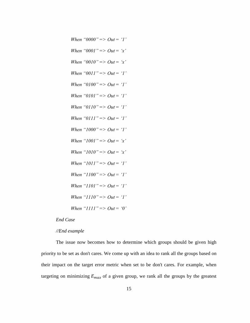
The method of introducing don't cares for designs in Verilog HDL is shown in

the following example. If power (both dynamic and leakage power) constraints and area

constraint are set to Synthesis Tools such as Synopsis Design Compiler [17], to simplify

the logic and minimize power and area, when In is “0001”, “0010”, “1001” or “1010”,

Out is set to be ‘1’ in these four cases, so the overall logic becomes

𝑂𝑢𝑡 = 𝐼𝑛[3] · 𝐼𝑛[2] · 𝐼𝑛[1] · 𝐼𝑛[0]̅̅ ̅̅ ̅̅ ̅̅ ̅̅ ̅̅ ̅̅ ̅̅ ̅̅ ̅̅ ̅̅ ̅̅ ̅̅ ̅̅ ̅̅ ̅̅ ̅

which generates the simplest logic. Otherwise, the logic will be much more complex,

thus consuming more power and area accordingly.

//An example of introducing don’t cares in Verilog HDL

//In: 4-bit variable

//Out: 1-bit variable

Case (In) is

15

When “0000” => Out = ‘1’

When “0001” => Out = ‘x’

When “0010” => Out = ‘x’

When “0011” => Out = ‘1’

When “0100” => Out = ‘1’

When “0101” => Out = ‘1’

When “0110” => Out = ‘1’

When “0111” => Out = ‘1’

When “1000” => Out = ‘1’

When “1001” => Out = ‘x’

When “1010” => Out = ‘x’

When “1011” => Out = ‘1’

When “1100” => Out = ‘1’

When “1101” => Out = ‘1’

When “1110” => Out = ‘1’

When “1111” => Out = ‘0’

End Case

//End example

The issue now becomes how to determine which groups should be given high

priority to be set as don't cares. We come up with an idea to rank all the groups based on

their impact on the target error metric when set to be don't cares. For example, when

targeting on minimizing 𝐸𝑚𝑎𝑥 of a given group, we rank all the groups by the greatest

16

value of 𝐸𝑚𝑎𝑥 because the compensation value which is the output of a group can be

assigned to be any value of a specific range for logic complexity simplification when set

to be don't cares. Then, the groups which have smaller greatest 𝐸𝑚𝑎𝑥 are given higher

priority to be set as don't cares, while other groups are implemented precisely because

they have comparatively larger 𝐸𝑚𝑎𝑥.

2.5 Practical ECU Design Guidance

The above theoretical analysis provides optimal design strategies for minimizing

a particular error metric. In practice, minimization of one error metric may often lead to

near-optimal minimization of other error metrics. We summarize the practical ECU

design guidance that is directly resulted from these results:

1) Different input groups shall have no or little overlap on the 𝐸𝐵𝐶,𝑖 axis to

minimize approximation error;

2) The 𝐸𝐵𝐶,𝑖 spread of each group shall be largely of equal length;

3) Non-uniformity of 𝐸𝐵𝐶,𝑖 spread may be reduced by splitting groups with a

large spread into smaller groups;

4) For a given compensation/grouping scheme, the optimal compensation values

for all groups can be determined to minimize a given error metric according

to Theorems 1-3.

5) Better accuracy performance can be achieved by introducing extra signatures

of certain input bits to divide large classes into small groups with different

compensation value for each group. Energy consumption and area can be

17

further reduced by introducing don't cares to some of the groups which have

comparatively small impact on the overall error.

18

3. PROPOSED MULTIPLIER DESIGN

The AAAC model is applied to approximate fixed-width Booth multiplier design

and its extension to full-width multipliers.

3.1 Fundamentals of Booth Multipliers

Booth multipliers are ideal for high speed applications and the Radix-4 Modified

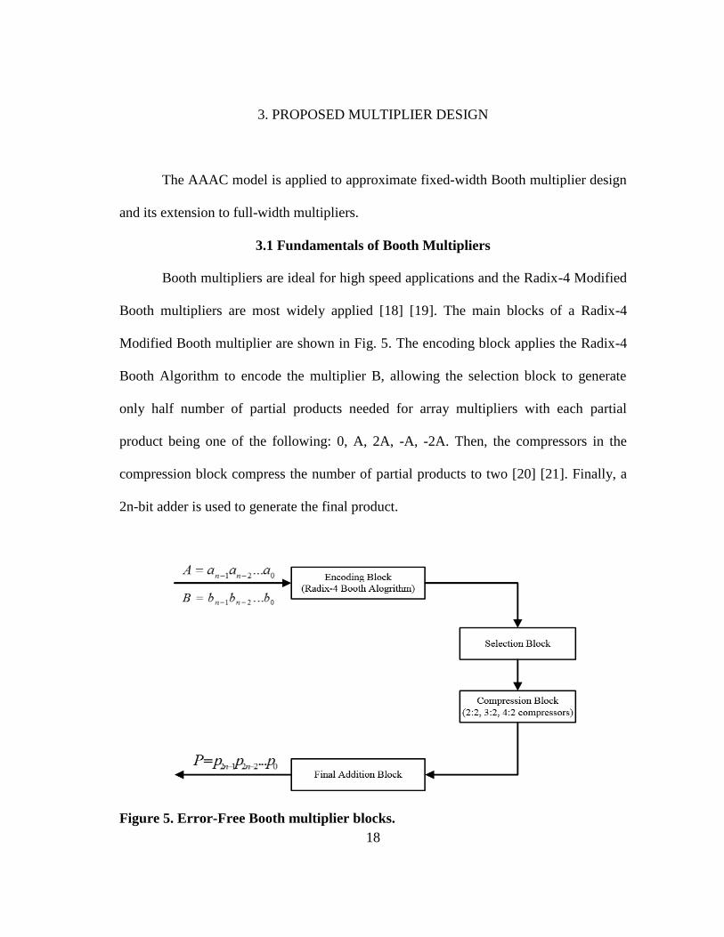
Booth multipliers are most widely applied [18] [19]. The main blocks of a Radix-4

Modified Booth multiplier are shown in Fig. 5. The encoding block applies the Radix-4

Booth Algorithm to encode the multiplier B, allowing the selection block to generate

only half number of partial products needed for array multipliers with each partial

product being one of the following: 0, A, 2A, -A, -2A. Then, the compressors in the

compression block compress the number of partial products to two [20] [21]. Finally, a

2n-bit adder is used to generate the final product.

Figure 5. Error-Free Booth multiplier blocks.

19

3.2 The Basic Idea

In this work, we use nxn fixed-width Booth multipliers to refer to approximate

Booth multipliers that operate on two n-bit inputs while outputting only an n-bit product

[4]. For convenience of discussion, we assume the higher and lower n bits of the

multiplicand and multiplier correspond to the integer and fractional parts of the inputs,

respectively. In this regard, a fixed-width multiplier outputs, possibly in an approximate

manner, the n-bit integer part of the exact product.

Fig. 6 shows the schematics of Radix-4 Booth encoding block applied in this

research, the outputs of encoding block are 𝑠𝑖, 𝑑𝑖, 𝑛𝑖, 𝑧𝑖 and 𝑐𝑖: (a) is the schematic of 𝑠𝑖,

𝑑𝑖 generation. (b) is the schematic of 𝑛𝑖 generation. (c) is the schematic of 𝑧𝑖 generation.

(d) is Schematic of 𝑐𝑖 generation.

𝑧𝑖 signifies whether the partial product is zero or not, 𝑛𝑖 specifies the sign of each

partial product, {𝑑𝑖 , 𝑠𝑖 } determines magnitude of the value multiplied by A for the

partial product (0, A or 2A), where 𝑑𝑖 is the more significant bit and 𝑠𝑖 is the less

significant bit. 𝑐𝑖 is the correction constant required to generate the negative partial

product.

𝑠𝑖, 𝑑𝑖, 𝑛𝑖, 𝑧𝑖 and 𝑐𝑖are generated by three consecutive input bits of multiplier B,

which are 𝑏2𝑖−1, 𝑏2𝑖 and 𝑏2𝑖+1.

Fig. 7 presents the schematic of the selection block applied in this research,

where 𝑝𝑝𝑖,𝑗 represents the 𝑗𝑡ℎ bit of 𝑖𝑡ℎ partial product.

20

(a)

(b)

(c)

(d)

Figure 6. Schematics of Radix-4 Booth encoding block: (a) Schematic of 𝒔𝒊 , 𝒅𝒊

generation, (b) Schematic of 𝒏𝒊 generation, (c) Schematic of 𝒛𝒊 generation, (d)

Schematic of 𝒄𝒊 generation.

21

Figure 7. Schematic of the selection block.

Fig. 8 shows the full 8-partial product array for a full-precision 16x16 bits Booth

multiplier where each dot row (𝑃𝑃0 to 𝑃𝑃7) is a partial product. The 16 dots (bits) in

each 𝑃𝑃𝑖 are denoted by 𝑝𝑝𝑖,15𝑝𝑝𝑖,14... 𝑝𝑝𝑖,10 from left to right. The vertical dashed line

splits the array at the position of the binary (radix) point. A fixed-width multiplier

outputs an integer output by approximating the carry-out produced by the fractional part

of the array, which is also labeled as the truncation part (TP). On the other hand, the

contribution of the bits left of the binary point, i.e., ones in the accurate part (AP), is not

approximated.

Figure 8. Partial product diagram for fixed-width 16x16 bits Booth multipliers

(n=16).

22

Direct-Truncated Booth multipliers (DTM) [5], which are an extreme case of

fixed-width multipliers, output an n-bit integer product by simply neglecting the bits in

the TP part of the array without forming them in the first place, thus potentially

producing a large error. As another extreme, Post-Truncated Booth multipliers (PTM)

[3] form the complete partial product array, compress all the bits, compute with full

precision, add an extra “1” to the 𝑛 − 1𝑡ℎ column to exactly round the carry-out to the

𝑛𝑡ℎ column, and finally output the exact n-bit integer part of the final product (with

rounding), as shown in Fig. 8. As such, PTMs are the most accurate fixed-width

multipliers.

Our goal in approximate fixed-width multiplier design is to approach the

accuracy of a PTM without incurring its high overhead that is commensurate with that of

a full-precision multiplier. Under the AAAC model, we associate the accurate part (AP)

and the truncation part (TP) of the array in Fig. 8 with the LPCU and ECU, respectively.

More specifically, the bits in AP are processed by the LPCU while the effects of the ones

in TP are approximated by the ECU in the form of error compensation. The exact

product (EFCU output) is

𝑂𝐸𝐹𝐶𝑈 = 𝑂𝐿𝑃𝐶𝑈 + 𝑆𝑇𝑃

where 𝑆𝑇𝑃 is the partial sum of TP, and 𝑂𝐿𝑃𝐶𝑈 is the LPCU output corresponding to AP.

To reduce the amount of approximate error, we further divide TP into 𝑇𝑃𝐻 (i.e., the

𝑛 − 1𝑡ℎ column) and 𝑇𝑃𝐿 and have

𝑆𝑇𝑃,𝐻 =1

2𝑆𝑈𝑀𝑛−1

23

𝑆𝑇𝑃,𝐿 =1

4𝑆𝑈𝑀𝑛−2 +

1

8𝑆𝑈𝑀𝑛−3 + ⋯ + (

1

2)𝑛𝑆𝑈𝑀0 (9)

where 𝑆𝑇𝑃,𝐻 and 𝑆𝑇𝑃,𝐿 correspond to the partial sums of 𝑇𝑃𝐻 and 𝑇𝑃𝐿 , and 𝑆𝑈𝑀𝑖

represents the sum of all bits in the 𝑖𝑡ℎ column, respectively. Now it is clear that

𝑆𝑇𝑃 = 𝑆𝑇𝑃,𝐻 + 𝑆𝑇𝑃,𝐿

The main objective in the design of ECU is to well approximate

𝑆𝑇𝑃 ≈ 𝑂𝐸𝐶𝑈

such that a fixed-width n-bit output is produced, i.e.,

𝑂𝐸𝐹𝐶𝑈 = 𝑂𝐿𝑃𝐶𝑈 + 𝑆𝑇𝑃 ≈ 𝑂𝐿𝑃𝐶𝑈 + 𝑂𝐸𝐶𝑈

Note again that the ECU of a PTM (most accurate fixed-width multiplier) produces as

the output (with rounding)

𝑂𝐸𝐶𝑈,𝑃𝑇𝑀 = 𝑖𝑛𝑡(𝑆𝑇𝑃 + 1) = 𝑖𝑛𝑡(𝑆𝑇𝑃,𝐻 + 𝑆𝑇𝑃,𝐿 + 1) (10)

where int(·) returns the integer part of its argument. To approach the PTM, we design

our ECU's output to be

𝑂𝐸𝐶𝑈 = 𝑖𝑛𝑡(𝑆𝑇𝑃,𝐻 + 𝑆𝑇𝑃,�̃� + 1) (11)

where 𝑆𝑇𝑃,�̃� is a good approximation to 𝑆𝑇𝑃,𝐿. In (11), only 𝑆𝑇𝑃,�̃� is approximated by the

ECU while 𝑆𝑇𝑃,𝐻 is computed exactly. Regarding to (11), we denote the carry-out from

𝑇𝑃𝐿 to 𝑇𝑃𝐻 by θ

𝜃 = 𝑖𝑛𝑡(2 · 𝑆𝑇𝑃,𝐿) (12)

(10) can now be simplified to

𝑂𝐸𝐶𝑈,𝑃𝑇𝑀 = 𝑖𝑛𝑡(𝑆𝑇𝑃,𝐻 +1

2θ + 1) (13)

24

Going back to (11), it is now clear that the main task of the ECU design is to well

approximate 𝜃. Since 𝑆𝑇𝑃,𝐻 is kept exact in (11), it is also natural to associate both AP

and 𝑆𝑇𝑃,𝐻 with the LPCU, and process them with the LPCU's encoding and selection

blocks. In this case, the ECU only produces an approximate 𝜃.

3.3 Design of Error Compensation Unit

According to Section 2.5, the key problem in the ECU design is to classify all

input patterns into largely equally sized groups with none or little overlap according to

values of 𝐸𝐵𝐶,𝑖, which is the error before compensation (in this case 𝜃).

To start, we first examine the standard Booth encoding that encodes each set of

three consecutive bits of multiplier B into five signals and determines the corresponding

partial product in terms of multiplicand A in Table 1, where 𝑧𝑖 signifies whether the

partial product is zero or not, 𝑛𝑖 specifies the sign of each partial product, {𝑑𝑖 , 𝑠𝑖 }

determines magnitude of the value multiplied by A for the partial product (0, A or 2A),

𝑐𝑖 is the correction constant required to generate the negative partial product and added

to the end of the partial product and 𝑃𝑃𝑖 is the actual 𝑖𝑡ℎ partial product generated from

the selection block.

As in Fig. 8, it is worth noting that Booth encoding is applied across the entire

partial product array including the TP part, which is associated with the error.

By following the ECU design guidance in Section 2.5, we identify a set of error

compensation signatures of low cost from Table 1, which shows signals of Radix-4

Booth encoding, to compensate for the error due to TP.

25

Input bits of Multiplier B

(for 𝑖𝑡ℎ partial product) Booth Encoder Outputs

(for 𝑖𝑡ℎ partial product)

Partial

Product

𝑏2𝑖+1 𝑏2𝑖 𝑏2𝑖−1 𝑧𝑖 𝑐𝑖 𝑛𝑖 𝑑𝑖 𝑠𝑖 𝑃𝑃𝑖

0 0 0 1 0 0 0 0 0

0 0 1 0 0 0 0 1 A

0 1 0 0 0 0 0 1 A

0 1 1 0 0 0 1 0 2A

1 0 0 0 1 1 1 0 -2A

1 0 1 0 1 1 0 1 -A

1 1 0 0 1 1 0 1 -A

1 1 1 1 0 1 0 0 0

Table 1. Signals of Radix-4 Booth encoding.

Our key idea is to use encoded sign and magnitude information of the partial

products to classify the input patterns into largely equally sized non-overlapping groups

according to the 𝐸𝐵𝐶,𝑖 value. In the following, we first present a set of error signatures

for each partial product, and then compress them for the entire ECU.

1) The first signature to be chosen is 𝑧𝑖. It is effective since a non-zero value of

𝑧𝑖 signifies the zero-valued corresponding partial product 𝑃𝑃𝑖 , thereby

classifying the inputs into two 𝐸𝐵𝐶,𝑖 (zero vs. non-zero error) groups

independently of the multiplicand A.

Starting from these two input groups, we select our second signature to be

𝑛𝑖, which encodes the sign of 𝑃𝑃𝑖, allowing us to further partition the large

non-zero 𝐸𝐵𝐶,𝑖 input group into two smaller groups of positive vs. negative

error.

To further reduce the approximation error, we introduce the third

signature to split the large signed error input groups by using the magnitude

26

information of each partial product. For this, we count the number of non-

zero bits in multiplicand A

𝑛𝑛𝑧𝑎 = ∑ 𝑎𝑖

𝑛−1

𝑖=0

2) Note that 𝑛𝑖 and 𝑧𝑖 are defined for each partial product and there are n/2

partial products for nxn bits multiplication. In addition, 𝑛𝑛𝑧𝑎 ranges from 0 to

n. Utilizing these signatures for the ECU would create a huge number of

input groups and lead to significant area and energy overhead. To simplify

the design of the signature generator, we first sum up 𝑛𝑖 and 𝑧𝑖 to produce

CA and CB, respectively, and then introduce a Boolean variable FA that

indicates whether 𝑛𝑛𝑧𝑎 is above n/2 or not

𝐶𝐴 = ∑ 𝑧𝑖

𝑛2

−1

𝑖=0

𝐶𝐵 = ∑ 𝑛𝑖

𝑛2

−1

𝑖=0

𝐹𝐴 = {0, ∑ 𝑎𝑖 <

𝑛

2

𝑛−1𝑖=0

1, ∑ 𝑎𝑖 ≥𝑛

2

𝑛−1𝑖=0

(14)

CA, CB and FA are the final set of compressed signatures we use

for the ECU. These signatures can be implemented with low-cost in

hardware. Fig. 9 illustrates the design of the proposed signature generator

that consists of two carry propagation adders (CPAs) for generating CA,

CB and an n-input odd-even sorting network [22] (Fig. 10) for FA

27

generation. Note that 𝑛𝑖 and 𝑧𝑖 are already computed by the encoders in

the LPCU.

Figure 9. Blocks and schematics of Signature Generator.

min max min max

min max min max

Figure 10. Blocks of sorting network.

28

3.4 The Complete Fixed-Width Multiplier

With the selected signatures and classified input groups, next, we need to

determine the actual error compensation for each group, i.e., an approximate to 𝜃 in (12).

As discussed in Section 2.3, one can follow Theorems 1-3 to choose a fixed

compensation for each input group to minimize a targeted error metric. For example, to

minimize 𝐸𝑚𝑠 , the optimal compensation is the average 𝑖𝑛𝑡(2 · 𝑆𝑇𝑃,𝐿) value for each

group. The ECU is designed to run in parallel with the selection block and part of

compression block so that it causes little extra delay during runtime.

We take 16x16 bits fixed-width Booth multiplier design as an example to

illustrate the signature and compensation generation schemes, and additional possible

simplifications. To further simplify the ECU, we consider different ranges and

combinations of the signature values in Table 2, where ∧ denotes AND operation. In

Table 2, the conditions of five cases are mainly determined by CA.

For CA in range [0, 1], when (𝐶𝐴 = 1)⋀(𝐶𝐵 < 3)⋀(𝐹𝐴 = 0) , the

corresponding input patterns belong to Case 1. The rest of input patterns when CA in

range [0, 1] belong to Case 2.

For CA in range [2, 5], when (𝐶𝐴 = 2)⋀(𝐶𝐵 > 3)⋀(𝐹𝐴 = 0) or (𝐶𝐴 =

2)⋀(𝐶𝐵 < 3)⋀(𝐹𝐴 = 1), the corresponding input patterns belong to Case 3. The rest of

input patterns when CA in range [2, 5] belong to Case 4.

For CA in range [6, 8], all input patterns belong to Case 5.

The goal is to identify a smaller set of refined input groups with controlled error

spread. 𝑆𝑇𝑃,𝐿 is the average of 𝑆𝑇𝑃,𝐿 in each input group.

29

Case 𝜃 𝑆𝑇𝑃,𝐿

1 1 0.9853

2 2 1.1259

3 2 1.0188

4 1 0.8580

5 0 0.4001

Table 2. Compensation for input groups of 16x16 multiplier.

To minimize 𝐸𝑚𝑠 , the optimal integer error compensation 𝜃 is set to be the

average of (8) in the group.

To further simplify, as shown in Table 3, the cases which have the same 𝜃 are

merged into the same group. Therefore, Case 2 and Case 3 are merged to form Group 1

(G1). Group 2 (G2) consists of Cases 1 and 4. Finally, Case 5 forms Group 3 (G3). Each

merged group has the same 𝜃 (average compensation value for all input cases in one

group) and error selection is realized by a simple 3-to-1 mux.

Group Number Case Number 𝜃 𝑆𝑇𝑃,𝐿

1 2, 3 2 1.1153

2 1, 4 1 0.8608

3 5 0 0.4001

Table 3. Optimal compensation for the refined input groups.

3.5 Proposed Full-Width Booth Multiplier

Approximate full-width multipliers, i. e., ones that approximate accurate nxn

Booth multipliers by outputting a full-width 2n-bit approximate product, are also useful

for many practical applications.

30

The presented fixed-width design can be readily extended to facilitate full-width

operation with the difference being that in this case we would like to approximate 𝑆𝑇𝑃,𝐿

by 𝑆𝑇𝑃,�̃� as in (11).

Again, to minimize 𝐸𝑚𝑠, for instance, the optimal compensation for each input

group would be the average of 𝑆𝑇𝑃,𝐿, denoted by 𝑆𝑇𝑃,𝐿, in that group. For n=16, we show

the values of 𝑆𝑇𝑃,𝐿 for the same three input groups in the last column of Table 3.

31

4. PROPOSED SQUARER DESIGN

4.1 The Basic Squarer Design

We demonstrate the application of the AAAC model to approximate fixed-width

squarers and its extension to full-width squarer designs.

Fig. 11 shows the full 8-partial squaring array (𝑃𝑆0 to 𝑃𝑆7) for a full-precision

16-bit squarer, where the input is denoted by A(𝑎𝑛−1 ... 𝑎0) [9].

Figure 11. Squaring diagram for 16-bit fixed-width squarers.

Here, we use the method in [9] to implement squarers instead of using Booth

algorithm as applied to multiplier design in Section 3 [9] because squarers implemented

by using the method in [9] are more energy-efficient and faster since most partial

products bits are implemented by simple AND operation of two input bits instead of

more complex Booth encoding and selection blocks.

32

The squarer design process is similar to the one presented for the proposed

multipliers (e.g., based on eqn. (9 - 13). Again, the key problem is to design an ECU to

well approximate 𝜃. By following the ECU design guidance in Section 2.5, we consider

the signals on the 𝑛 − 2𝑡ℎ column as signatures since they have the highest weight on

𝑇𝑃𝐿 and include all input bits which contribute to 𝑇𝑃𝐿.

To simplify the design of the signature generator, we sum up the signals on the

𝑛 − 2𝑡ℎ column to produce the first signature CA. We introduce one input bit as the

second signature (CB) to further split the large input groups formed by CA. Accordingly,

input bit 𝑎6 is chosen as the second signature CB for the proposed 16-bit squarer.

The final input cases of the 16 bit squarer classified by CA and CB are show in

Table 4. CA is generated by an odd-even sorting network [22], which has a low

hardware overhead, and CB is selected directly from the input A. The error

compensations 𝜃 for the fixed-width squarer are shown in the second last column of

Table 4. The values of 𝑆𝑇𝑃,𝐿 (error compensation) of different input cases for the full-

width squarer are shown in the last column of Table 4.

Case Condition 𝜃 𝑆𝑇𝑃,𝐿

1 𝐶𝐴 = 0 0 0.2197

2 (𝐶𝐴 = 1)⋀(𝐶𝐵 = 0) 0 0.4539

3 (𝐶𝐴 = 1)⋀(𝐶𝐵 = 1) 1 0.6210

4 (𝐶𝐴 = 2)⋀(𝐶𝐵 = 0) 1 0.8133

5 (𝐶𝐴 = 2)⋀(𝐶𝐵 = 1) 2 1.0134

6 𝐶𝐴 = 3 2 1.2902

7 𝐶𝐴 = 4 3 1.6966

8 𝐶𝐴 = 5 4 2.1278

9 𝐶𝐴 = 6 5 2.5838

10 𝐶𝐴 = 7 6 3.0645

Table 4. Compensation for input cases of 16-bit squarer.

33

According to 𝜃 in different input cases, for 16-bit fixed-width squarer design, we

combine them into seven groups, which are shown in Table 5. Case 1 and case 2 are

merged to group 1. Case 3 and Case 4 form group 2. Group 3 consists of case 5 and case

6. Then case 7 becomes group 4, case 8 becomes group 5, case 9 becomes group 6 and

finally, case 10 becomes group 7.

Group Case 𝜃

1 1, 2 0

2 3, 4 1

3 5, 6 2

4 7 3

5 8 4

6 9 5

7 10 6

Table 5. Compensation for input groups of 16-bit squarer.

4.2 Further Error and Cost Reduction for Fixed-Width Squarers

As described in Section 2.4, we may introduce extra signatures of certain input

bits to sub-divide each of the large input classes into groups to further reduce one or

more error metrics. To further simplify the logic, thus decreasing energy consumption

and area of ECU after introducing extra signatures, don't cares are added for certain

input groups.

Now we introduce extra signatures and don't cares to further decrease 𝐸𝑚𝑎𝑥 as

well as energy consumption and area for the proposed 16-bit fixed-width squarer. To

give an overall evaluation of designs, an energy-delay-max error product is defined as

𝐸𝑛𝑒𝑟𝑔𝑦 · 𝐷𝑒𝑙𝑎𝑦 · 𝐸𝑚𝑎𝑥 (𝐸𝐷𝐸𝑚𝑎𝑥).

34

First, we introduce extra input signatures. In the proposed 16-bit fixed-width

squarer design, input bit 𝑎6 is utilized as one signature because it can further divide

some of the large eight classes formed by signature CA into groups. Specifically, we try

each input bit from 𝑎0 to 𝑎15 according to the design guidance in Section 2 that an

efficient signature should be able to divide input cases into groups largely of equal

length (sub-dividing large input classes formed by the first signature CA in this case).

The simulation results indicate that selecting 𝑎6as a signature can divide more large

original groups formed by the first signature CA and achieve better overall accuracy

performance than other input bit from 𝑎0 to 𝑎15. Using the same method, the second

extra signature is chosen after the generation of the signatures of CA and 𝑎6.

Table 22 lists the number of extra signatures and the corresponding signatures

chosen from 16 input bits (𝑎0 to 𝑎15). Note that for 16-bit fixed-width squarer design,

the number of extra signatures considered is no more than seven because when the

number of extra signatures reaches eight or goes beyond eight, energy consumption and

area increase very rapidly. At the same time, the obtained improvement on 𝐸𝑚𝑎𝑥 is

limited such that 𝐸𝐷𝐸𝑚𝑎𝑥 becomes much bigger.

Second, to further decrease energy consumption and area, as illustrated in Sub-

section 2.4, don't cares are introduced to some of groups. Considering about logic

complexity, if the compensations for all the groups formed by signatures of CA and

extra signatures are implemented precisely, an ECU with a complex logic will be

generated through logic synthesis, though the error may be minimized. In order to

simplify ECU design and tradeoff between cost and error, we set compensation values of

35

some groups which don’t contribute much of the overall error to be don’t cares so that

the overall error won’t be increased dramatically.

For example, to minimize overall 𝐸𝑚𝑎𝑥, we may rank the groups based on their

greatest 𝐸𝑚𝑎𝑥 , which is defined as the biggest 𝐸𝑚𝑎𝑥 that the groups can reach when

𝜃 is any value in its range. Since 𝜃 has three bits in this case, it ranges from 0 to 7 in

decimal number. After the groups are ranked by greatest 𝐸𝑚𝑎𝑥, those which have smaller

greatest 𝐸𝑚𝑎𝑥 are given a higher priority to be set as don't cares.

In practice, the more don't cares we set, the less energy consumption and area the

design can achieve with the use of a logic synthesis tool such as Synopsis Design

Compiler [22], and the bigger 𝐸𝑚𝑎𝑥 it is likely to have. Therefore, the number of don't

care set for groups should be chosen by jointly considering based on the specifications of

energy, delay, area and 𝐸𝑚𝑎𝑥 (or other targeted error metric).

36

5. COMPRESSORS FOR MULTIPLIER AND SQUARER DESIGN

Fig. 12 shows the complete design of the proposed multiplier (a), the details of

which is presented in Section 3, and the proposed squarer (b), the details of which is

presented in Section 4. For proposed multiplier design, the encoding block applies the

Radix-4 Booth Algorithm to encode the multiplier B, allowing the selection block to

generate only half number of partial products needed for array multipliers with each

product being one of the following: 0, A, 2A, -A, -2A (shown in Fig. 8). For the

proposed squarer design, the similar partial product table shown in Fig. 11 is generated.

After the dots which stand for partial products and contain AP, 𝑇𝑃𝐻 and

𝜃 (for fixed-width designs) or 𝑆𝑇𝑃,𝐿 (for full-width designs), shown in Fig. 8 for

multipliers and Fig. 11 for squarers, are generated, they are compressed to only two

partial products by compressors in the compression block. Finally, the two partial

products are fed into the final adding block and the final result is generated using a Carry

propagation adder (CPA).

The purpose of using compressors in the compression block is that multiple

compressors can run in parallel, thus speeding up the compression process. In this

section, we discuss three types of comparatively low-cost compressors (2:2 Compressors

[20], 3:2 Compressors [20] and 4:2 Compressors [21]) that are used in the proposed

multiplier and squarer design because they have comparatively less energy and delay

overhead. We also discuss the processing steps involved in compression in which

multiple compressors run in parallel.

37

(a)

(b)

Figure 12. Complete designs blocks: (a) the proposed multipliers, (b) the proposed

squarers.

5.1 2:2 Compressors

2:2 Compressors have the same function as half adders. 2:2 Compressors help to

compress two 1-bit inputs into one 2-bit output. The logic function of 2:2 compressors is

presented below

in1

+ in2

out2 out1

𝑜𝑢𝑡1 = 𝑖𝑛1 ⨁𝑖𝑛2

𝑜𝑢𝑡2 = 𝑖𝑛1 ∧ 𝑖𝑛2

38

where in1, in2 are 1-bit inputs, {out2, out1} is the 2-bit output and ⨁ denotes ‘xor’

operation, the block of 2:2 compressors is shown in Fig. 13.

Half Adder

(HA)

in1

in2

{out2,out1}

Figure 13. Block diagram of a 2:2 compressor.

5.2 3:2 Compressors

3:2 Compressors [20] have the same function as full adders. 3:2 Compressors

help to compress three 1-bit inputs into one 2-bit output. The logic function of 3:2

compressors is presented below

in1

in2

+ in3

out2 out1

𝑜𝑢𝑡1 = 𝑖𝑛1 ⨁𝑖𝑛2⨁𝑖𝑛3

𝑜𝑢𝑡2 = 𝑖𝑛1 ∧ 𝑖𝑛2 ∧ 𝑖𝑛3

where in1, in2 and in3 are 1-bit inputs, {out2, out1} is the 2-bit output, the block of 3:2

compressors is shown in Fig. 14.

Full Adder

(FA)

in1

in3

{out2,out1}in2

Figure 14. Blocks of a 3:2 compressor.

39

5.3 4:2 (5:3) Compressors

The logic function of 4:2 (5:3) compressors [21] is presented below. 4:2

compressors have better speed performance than 2:2 and 3:2 compressors but with

higher energy consumption and area overhead.

in1

in2

in3

in4

+ in5

out2 out1

out3

𝑜𝑢𝑡1 = 𝑖𝑛1 ⨁𝑖𝑛2⨁𝑖𝑛3⨁𝑖𝑛4⨁𝑖𝑛5

𝑜𝑢𝑡2 = (𝑖𝑛4 ∧ 𝑖𝑛5) ∨ (𝑖𝑛1 ⨁𝑖𝑛2⨁𝑖𝑛3) ∨ ((𝑖𝑛1 ⨁𝑖𝑛2⨁𝑖𝑛3) ∧ 𝑖𝑛5)

𝑜𝑢𝑡3 = (𝑖𝑛1 ∧ 𝑖𝑛2) ∨ (𝑖𝑛2 ∧ 𝑖𝑛3) ∨ (𝑖𝑛1 ∧ 𝑖𝑛3)

where in1, in2, in3, in4 and in5 are 1-bit inputs, {out2+out3, out1} is the output and ∨

denotes ‘or’ operation.

5.4 Using Compressors to Compress Array-Based Partial Product Table

2:2, 3:2 [20] and 4:2 [21] compressors are applied to the compression block

shown in Fig. 13 to compress array-based partial product table such as those shown in

Fig. 8 and Fig. 11.

As is presented in early this section, the reason why compressors are used in the

compression block is that multiple compressors can run in parallel so that the

40

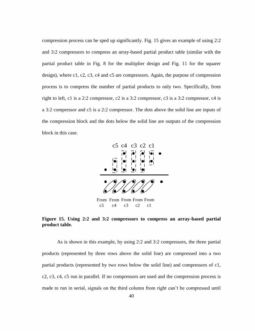
compression process can be sped up significantly. Fig. 15 gives an example of using 2:2

and 3:2 compressors to compress an array-based partial product table (similar with the

partial product table in Fig. 8 for the multiplier design and Fig. 11 for the squarer

design), where c1, c2, c3, c4 and c5 are compressors. Again, the purpose of compression

process is to compress the number of partial products to only two. Specifically, from

right to left, c1 is a 2:2 compressor, c2 is a 3:2 compressor, c3 is a 3:2 compressor, c4 is

a 3:2 compressor and c5 is a 2:2 compressor. The dots above the solid line are inputs of

the compression block and the dots below the solid line are outputs of the compression

block in this case.

c1c2c3c4c5

From

c1

From

c2

From

c3

From

c4

From

c5

Figure 15. Using 2:2 and 3:2 compressors to compress an array-based partial

product table.

As is shown in this example, by using 2:2 and 3:2 compressors, the three partial

products (represented by three rows above the solid line) are compressed into a two

partial products (represented by two rows below the solid line) and compressors of c1,

c2, c3, c4, c5 run in parallel. If no compressors are used and the compression process is

made to run in serial, signals on the third column from right can’t be compressed until

41

the carry-out of the second column from the right is calculated and added to the third

column from right, the compression of the fourth column from the right is delayed by the

third column from the right, and the compression of the fifth column from the right has

to wait for the carry-out generated by the compression of fourth column from the right.

42

6. EXPERIMENTAL RESULTS

The proposed 16-bit fixed-width Booth multiplier and squarer are designed in

Verilog HDL, synthesized using Synopsis Design Compiler [17] with a commercial 90

nm CMOS technology and standard cell library. From Synopsis Design Compiler

synthesis (Design Vision) reports, we get the pre-layout delay, dynamic power, leakage

power and area.

We also implement four additional fixed-width Booth multipliers: DTM (Direct

Truncated Booth Multiplier) [5], PEBM (with probabilistic estimation bias

compensation) [8], ZSM (uses sum of iz as signatures) [7] and PTM (Post Truncated

Booth Multiplier — — most accurate/expensive fixed-width multiplier) [3] for

comparison purposes.

Four additional squarers are implemented: DTS (Direct Truncated Squarer), CCS

(with a constant compensation) [9], VCS (the signals on the 𝑛 − 2𝑡ℎ column as the

compensation) [10] and PTS (Post Truncated Squarer —— most accurate/expensive

fixed-width squarer).

For all Booth multiplier and squarer designs implemented in this research, partial

products are generated and then compressed to two partial products using 2:2, 3:2 [20]

and 4:2 [21] compressors. As demonstrated in Section 5, 2:2, 3:2 and 4:2 compressors

provide an efficient method for compressing the number of partial products to two

because they enable the compression process to run in parallel.

43

Finally, the two compressed partial products are added up by a carry propagation

adder (CPA) to produce final results.

6.1 Comparison of Different Multipliers

In Table 6, five fixed-width multipliers are compared in terms of area, delay,

power (sum of dynamic power and leakage power), energy and 𝐸𝑚𝑠.

The energy consumption and area of the proposed 16-bit fixed-width multiplier

are slightly larger than PEBM and ZSM, but are much smaller than PTM, with a 44.85%

and 28.33% reduction respectively. On the other hand, the proposed design has a

significantly reduced 𝐸𝑚𝑠 compared with DTM, PEBM and ZSM. This indicates that our

design delivers a much improved accuracy with a very small amount of additional

overhead compared with PEBM and ZSM. A detailed accuracy comparison will be given

in the next section.

Multiplier Area

(𝑢𝑚2)

Delay

(ns)

Power

(mW)

Energy

(pJ) 𝐸𝑚𝑠

DTM 2,645 2.61 0.86 2.24 9.85

PTM 5,239 3.72 1.75 6.51 0.08

PEBM 2,937 2.79 0.98 2.73 0.35

ZSM 3,256 2.99 1.11 3.32 0.20

Proposed 3,755 2.99 1.20 3.59 0.15

Table 6. Implementation results of different 16x16 bits fixed-width Booth

multipliers.

In order to give an overall comparison between the proposed fixed-width 16x16

multiplier design and other approximate fixed-width Booth multipliers, an energy-delay-

mean square error product 𝐸𝑛𝑒𝑟𝑔𝑦 · 𝐷𝑒𝑙𝑎𝑦 · 𝐸𝑚𝑠 (𝐸𝐷𝐸𝑚𝑠) is introduced to evaluate

different approximate designs.

44

Table 7 lists the 𝐸𝐷𝐸𝑚𝑠 of DTM, PTM, PEBM, ZSM and the proposed 16-bit

fixed width Booth multiplier. Fig. 16 lists the 𝐸𝐷𝐸𝑚𝑠 reduction of the proposed 16x16

bits fixed-width multipliers over DTM, PTM, PEBM and ZSM.

Multiplier 𝐸𝐷𝐸𝑚𝑠 (pJ ∙ ns)

DTM 57.59

PTM 1.94

PEBM 2.67

ZSM 1.99

Proposed 1.61

Table 7. 𝑬𝑫𝑬𝒎𝒔 of 16x16 fixed-width multipliers.

Figure 16. 𝑬𝑫𝑬𝒎𝒔 reduction of the proposed 16x16 bits fixed-width multipliers over

DTM, PTM, PEBM and ZSM.

0.00%

5.00%

10.00%

15.00%

20.00%

25.00%

30.00%

35.00%

40.00%

45.00%

50.00%

55.00%

60.00%

65.00%

70.00%

75.00%

80.00%

85.00%

90.00%

95.00%

100.00%

DTM PTM PEBM ZSM

45

The proposed multiplier has a significantly reduced 𝐸𝐷𝐸𝑚𝑠 compared with

DTM, PTM, PEBM and ZSM, with 97.20% reduction over DTM, 17.01% reduction

over PTM, 39.70% reduction over PEBM and 19.10% reduction over ZSM, respectively.

Therefore, the proposed 16-bit multiplier has the best overall performance among the

five existing approximate Booth multiplier designs.

6.2 Accuracy Analysis for the Approximate Multipliers

In this section, we provide a more detailed accuracy comparison among different

approximate multipliers. Error reduction or accuracy improvement of the proposed

design over the existing designs is defined as |𝐸𝑒𝑥𝑖𝑠𝑡𝑖𝑛𝑔−𝐸𝑝𝑟𝑝𝑜𝑠𝑒𝑑|

𝐸𝑒𝑥𝑖𝑠𝑡𝑖𝑛𝑔× 100%, where 𝐸𝑒𝑥𝑖𝑠𝑡𝑖𝑛𝑔

is one of error metrics (𝐸𝑎𝑣𝑒 , 𝐸𝑚𝑎𝑥 and 𝐸𝑚𝑠 ) of the compared existing design and

𝐸𝑝𝑟𝑜𝑝𝑜𝑠𝑒𝑑 is defined as one of error metrics (𝐸𝑎𝑣𝑒 , 𝐸𝑚𝑎𝑥 and 𝐸𝑚𝑠 ) of the proposed

design.

6.2.1 Fixed-Width Booth Multipliers

We evaluate the accuracies of the five different designs in terms of 𝐸𝑎𝑣𝑒, 𝐸𝑚𝑎𝑥

and 𝐸𝑚𝑠 (Section 2.1) for n = 8 (bits) in Table 8.

Multiplier 𝐸𝑎𝑣𝑒 𝐸𝑚𝑎𝑥 𝐸𝑚𝑠

DTM 1.50 4.00 2.69

PTM 0.25 0.50 0.08

PEBM 0.35 1.50 0.18

ZSM 0.30 1.17 0.14

Proposed 0.29 1.00 0.13

Table 8. Error metrics of 8x8 fixed-width Booth multipliers.

46

Fig. 17 shows the error reductions of the proposed fixed-width Booth multiplier

over DTM, PEBM and ZSM for n = 8 (bits). The achieved reductions are 3.33%,

14.53% and 7.14% in terms of 𝐸𝑎𝑣𝑒, 𝐸𝑚𝑎𝑥 and 𝐸𝑚𝑠, respectively, when compared with

ZSM.


DTM, PEBM, ZSM.


DTM 2.25 6.00 5.71

PTM 0.25 0.50 0.08

PEBM 0.40 2.00 0.25

ZSM 0.33 1.67 0.17

Proposed 0.30 1.46 0.14


0.00%

5.00%

10.00%

15.00%

20.00%

25.00%

30.00%

35.00%

40.00%

45.00%

50.00%

55.00%

60.00%

65.00%

70.00%

75.00%

80.00%

85.00%

90.00%

95.00%

100.00%

Average Error Max Error Mean Square Error

DTM

PEBM

ZSM

47

Then, we evaluate the accuracies of the five different designs in terms of 𝐸𝑎𝑣𝑒,

𝐸𝑚𝑎𝑥 and 𝐸𝑚𝑠 (Section 2.1) for n = 12 (bits) in Table 9.

Fig. 18 shows the significant error reductions of the proposed fixed-width

multipliers over DTM, PEBM and ZSM for n = 12 (bits). The achieved reductions are

9.09%, 12.57% and 17.65% in terms of 𝐸𝑎𝑣𝑒 , 𝐸𝑚𝑎𝑥 and 𝐸𝑚𝑠 , respectively, when

compared with ZSM.


DTM, PEBM, ZSM.


DTM 3.00 8.00 9.85

PTM 0.25 0.50 0.08

PEBM 0.48 2.50 0.35

ZSM 0.36 2.17 0.20

Proposed 0.32 1.56 0.15


0.00%5.00%

10.00%15.00%20.00%25.00%30.00%35.00%40.00%45.00%50.00%55.00%60.00%65.00%70.00%75.00%80.00%85.00%90.00%95.00%

100.00%


DTM

PEBM

ZSM

48

Besides, we evaluate the accuracies of the five different designs in terms of 𝐸𝑎𝑣𝑒,





compared with ZSM.


DTM, PEBM, ZSM.

Lastly, to evaluate the performance of our approach for much wider multipliers,

we evaluate the accuracies of the five different designs in terms of 𝐸𝑎𝑣𝑒, 𝐸𝑚𝑎𝑥 and 𝐸𝑚𝑠

(Section 2.1) for n = 32 (bits). Since the number of input cases is very large, exact error

0.00%

5.00%

10.00%

15.00%

20.00%

25.00%

30.00%

35.00%

40.00%

45.00%

50.00%

55.00%

60.00%

65.00%

70.00%

75.00%

80.00%

85.00%

90.00%

95.00%

100.00%


DTM

PEBM

ZSM

49

analysis becomes extremely time-consuming. To alleviate the computational challenge

while getting decent error estimates, we evaluate each error metric by averaging over a

large number of input combinations as follows. For example, for 𝐸𝑎𝑣𝑒 evaluation, we

first randomly generate one data set of 400 million input combinations and calculate

𝐸𝑎𝑣𝑒 for this set. To give a more decent and accurate error estimates, we randomly

generate 10 such data sets in total, with 400 million input combinations for each set, and

calculate the average 𝐸𝑎𝑣𝑒 of the ten sets and get the final 𝐸𝑎𝑣𝑒 result.




compared with ZSM.


DTM, PEBM, ZSM.

0.00%5.00%

10.00%15.00%20.00%25.00%30.00%35.00%40.00%45.00%50.00%55.00%60.00%65.00%70.00%75.00%80.00%85.00%90.00%95.00%

100.00%


DTM

PEBM

ZSM

50

6.2.2 Full-Width Booth Multipliers

We further evaluate the accuracies of the five different designs operated in full-

width mode in terms of 𝐸𝑎𝑣𝑒, 𝐸𝑚𝑎𝑥 and 𝐸𝑚𝑠 (Section 2.1) for n = 8 (bits) in Table 11.


PEBM 0.28 1.25 0.12

ZSM 0.21 0.95 0.07

Proposed 0.17 0.59 0.04

Table 11. Error metrics of 8x8 full-width Booth multipliers.

Fig. 21 shows the significant error reductions of the proposed full-width

multipliers over PEBM and ZSM for n = 8. The achieved reductions are 19.05%,


ZSM. Additionally, the proposed full-width outperforms the most accurate fixed-width

PTM with an error reduction of 32.00% and 50.00% for 𝐸𝑎𝑣𝑒 and 𝐸𝑚𝑠 , respectively,

when n = 8 (bits).


PEBM, ZSM.

0.00%5.00%

10.00%15.00%20.00%25.00%30.00%35.00%40.00%45.00%50.00%55.00%60.00%65.00%70.00%75.00%80.00%85.00%90.00%95.00%

100.00%


PEBM

ZSM

51

Then, we evaluate the accuracies of the five different designs operated in full-



PEBM 0.33 1.88 0.17

ZSM 0.25 1.48 0.10

Proposed 0.22 1.10 0.07



multipliers over PEBM and ZSM for n = 12. The achieved reductions are 12.00%,




when n = 12 (bits).


PEBM, ZSM.

0.00%5.00%

10.00%15.00%20.00%25.00%30.00%35.00%40.00%45.00%50.00%55.00%60.00%65.00%70.00%75.00%80.00%85.00%90.00%95.00%

100.00%


PEBM

ZSM

52

We evaluate the accuracies of the five different designs operated in full-width

mode in terms of 𝐸𝑎𝑣𝑒, 𝐸𝑚𝑎𝑥 and 𝐸𝑚𝑠 (Section 2.1) for n = 16 (bits) in Table 13.


PEBM 0.38 2.50 0.22

ZSM 0.29 2.00 0.13

Proposed 0.22 1.25 0.07



multipliers over PEBM and ZSM for n = 16 (bits). The achieved reductions are 24.14%,




when n = 16 (bits).


PEBM, ZSM.

0.00%5.00%

10.00%15.00%20.00%25.00%30.00%35.00%40.00%45.00%50.00%55.00%60.00%65.00%70.00%75.00%80.00%85.00%90.00%95.00%

100.00%


PEBM

ZSM

53

Lastly, to evaluate the performance of our approach for much wider multipliers,

we evaluate the accuracies of the five different designs in terms of 𝐸𝑎𝑣𝑒, 𝐸𝑚𝑎𝑥 and 𝐸𝑚𝑠

(Section 2.1) for n = 32 (bits). Similar to the proposed 32x32 fixed-width multiplier,

since the number of input cases is very large, exact error analysis becomes extremely

time-consuming. To alleviate the computational challenge while getting decent error

estimates, we evaluate each error metric by averaging over a large number of input

combinations as follows. For example, for 𝐸𝑎𝑣𝑒 evaluation, we first randomly generate

one data set of 400 million input combinations and calculate 𝐸𝑎𝑣𝑒 for this set. To give a

more decent and accurate error estimates, we randomly generate 10 such data sets in

total, with 400 million input combinations for each set, and calculate the average 𝐸𝑎𝑣𝑒 of

the ten sets and get the final 𝐸𝑎𝑣𝑒 result.


PEBM, ZSM.

0.00%5.00%

10.00%15.00%20.00%25.00%30.00%35.00%40.00%45.00%50.00%55.00%60.00%65.00%70.00%75.00%80.00%85.00%90.00%95.00%

100.00%


PEBM

ZSM

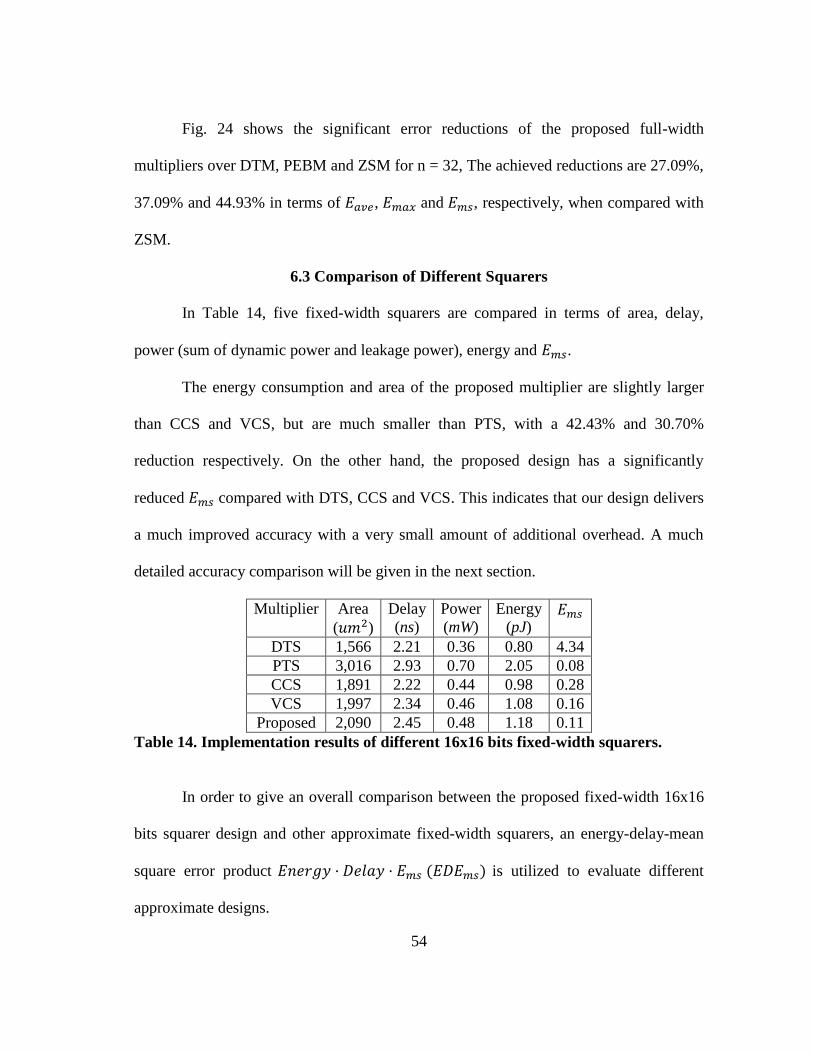
54


multipliers over DTM, PEBM and ZSM for n = 32, The achieved reductions are 27.09%,


ZSM.

6.3 Comparison of Different Squarers

In Table 14, five fixed-width squarers are compared in terms of area, delay,

power (sum of dynamic power and leakage power), energy and 𝐸𝑚𝑠.

The energy consumption and area of the proposed multiplier are slightly larger

than CCS and VCS, but are much smaller than PTS, with a 42.43% and 30.70%

reduction respectively. On the other hand, the proposed design has a significantly

reduced 𝐸𝑚𝑠 compared with DTS, CCS and VCS. This indicates that our design delivers

a much improved accuracy with a very small amount of additional overhead. A much

detailed accuracy comparison will be given in the next section.

Multiplier Area

(𝑢𝑚2)

Delay

(ns)

Power

(mW)

Energy

(pJ) 𝐸𝑚𝑠

DTS 1,566 2.21 0.36 0.80 4.34

PTS 3,016 2.93 0.70 2.05 0.08

CCS 1,891 2.22 0.44 0.98 0.28

VCS 1,997 2.34 0.46 1.08 0.16

Proposed 2,090 2.45 0.48 1.18 0.11

Table 14. Implementation results of different 16x16 bits fixed-width squarers.

In order to give an overall comparison between the proposed fixed-width 16x16

bits squarer design and other approximate fixed-width squarers, an energy-delay-mean

square error product 𝐸𝑛𝑒𝑟𝑔𝑦 · 𝐷𝑒𝑙𝑎𝑦 · 𝐸𝑚𝑠 (𝐸𝐷𝐸𝑚𝑠) is utilized to evaluate different

approximate designs.

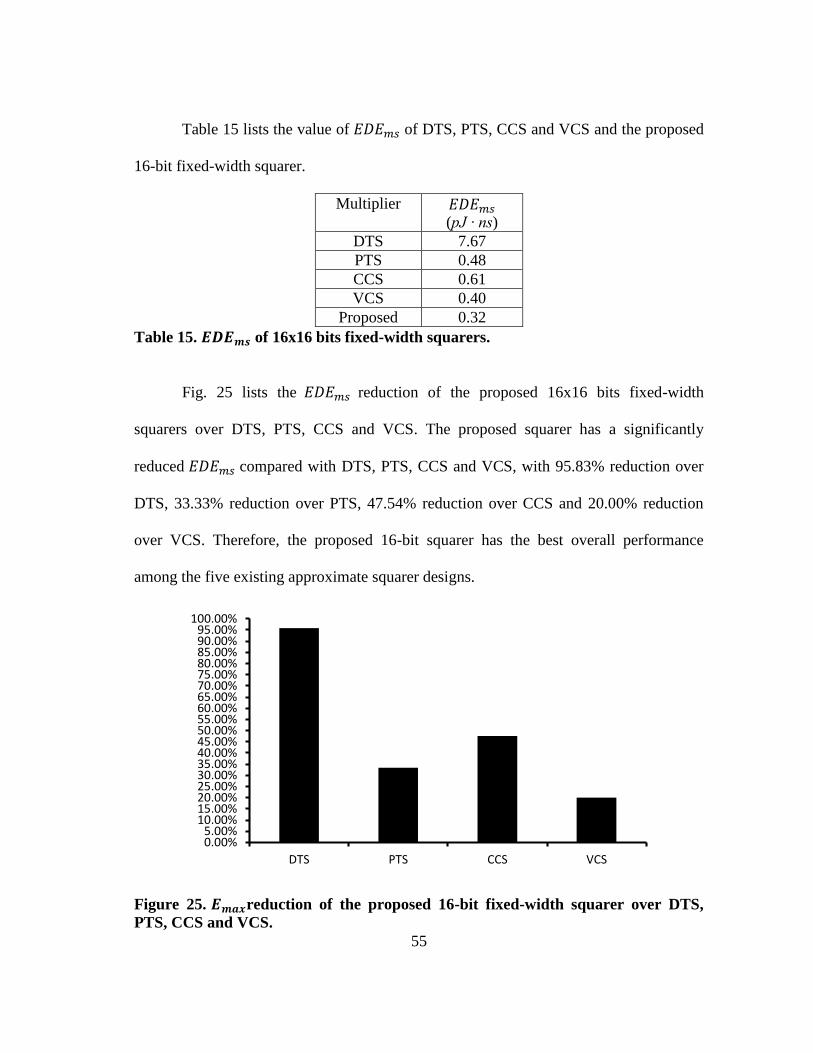
55

Table 15 lists the value of 𝐸𝐷𝐸𝑚𝑠 of DTS, PTS, CCS and VCS and the proposed

16-bit fixed-width squarer.

Multiplier 𝐸𝐷𝐸𝑚𝑠 (pJ ∙ ns)

DTS 7.67

PTS 0.48

CCS 0.61

VCS 0.40

Proposed 0.32

Table 15. 𝑬𝑫𝑬𝒎𝒔 of 16x16 bits fixed-width squarers.

Fig. 25 lists the 𝐸𝐷𝐸𝑚𝑠 reduction of the proposed 16x16 bits fixed-width

squarers over DTS, PTS, CCS and VCS. The proposed squarer has a significantly

reduced 𝐸𝐷𝐸𝑚𝑠 compared with DTS, PTS, CCS and VCS, with 95.83% reduction over

DTS, 33.33% reduction over PTS, 47.54% reduction over CCS and 20.00% reduction

over VCS. Therefore, the proposed 16-bit squarer has the best overall performance

among the five existing approximate squarer designs.

Figure 25. 𝑬𝒎𝒂𝒙reduction of the proposed 16-bit fixed-width squarer over DTS,

PTS, CCS and VCS.

0.00%5.00%

10.00%15.00%20.00%25.00%30.00%35.00%40.00%45.00%50.00%55.00%60.00%65.00%70.00%75.00%80.00%85.00%90.00%95.00%

100.00%

DTS PTS CCS VCS

56

6.4 Accuracy Analysis for Squarers

In this section, we provide a more detailed accuracy comparison among different

approximate squarers. Similar to multipliers, error reduction or accuracy improvement of

the proposed squarer design over the existing designs is defined as |𝐸𝑒𝑥𝑖𝑠𝑡𝑖𝑛𝑔−𝐸𝑝𝑟𝑝𝑜𝑠𝑒𝑑|

𝐸𝑒𝑥𝑖𝑠𝑡𝑖𝑛𝑔×

100%, where 𝐸𝑒𝑥𝑖𝑠𝑡𝑖𝑛𝑔 is one of error metrics (𝐸𝑎𝑣𝑒 , 𝐸𝑚𝑎𝑥 and 𝐸𝑚𝑠) of the compared

existing design and 𝐸𝑝𝑟𝑜𝑝𝑜𝑠𝑒𝑑 is defined as one of error metrics (𝐸𝑎𝑣𝑒, 𝐸𝑚𝑎𝑥 and 𝐸𝑚𝑠) of

the proposed squarer design.

6.4.1 Fixed-Width Squarers

We evaluate the accuracies of the five different designs in terms of 𝐸𝑎𝑣𝑒, 𝐸𝑚𝑎𝑥

and 𝐸𝑚𝑠 (Section 2.1) for n = 8 (bits) in Table 16.


DTS 0.83 3.00 1.10

PTS 0.23 0.50 0.08

CCS 0.28 1.10 0.13

VCS 0.29 0.88 0.13

Proposed 0.24 0.75 0.09

Table 16. Error metrics of 8-bit fixed-width squarers.


squarers over DTS, CCS and VCS for n = 8 (bits). The achieved reductions are 17.24%,


VCS.

Then, we evaluate the accuracies of the five different designs in terms of 𝐸𝑎𝑣𝑒,


57




VCS.


CCS, VCS.

0.00%

5.00%

10.00%

15.00%

20.00%

25.00%

30.00%

35.00%

40.00%

45.00%

50.00%

55.00%

60.00%

65.00%

70.00%

75.00%

80.00%

85.00%

90.00%

95.00%

100.00%


DTS

CCS

VCS

58


DTS 1.33 5.00 2.46

PTS 0.25 0.50 0.08

CCS 0.40 1.57 0.24

VCS 0.31 1.04 0.15

Proposed 0.26 0.88 0.10



CCS, VCS.

Lastly, we evaluate the accuracies of the five different designs in terms of 𝐸𝑎𝑣𝑒,


0.00%

5.00%

10.00%

15.00%

20.00%

25.00%

30.00%

35.00%

40.00%

45.00%

50.00%

55.00%

60.00%

65.00%

70.00%

75.00%

80.00%

85.00%

90.00%

95.00%

100.00%


DTS

CCS

VCS

59


DTS 1.83 7.00 4.34

PTS 0.25 0.50 0.08

CCS 0.42 2.56 0.28

VCS 0.33 1.20 0.16

Proposed 0.27 0.94 0.11





VCS.


CCS, VCS.

0.00%

5.00%

10.00%

15.00%

20.00%

25.00%

30.00%

35.00%

40.00%

45.00%

50.00%

55.00%

60.00%

65.00%

70.00%

75.00%

80.00%

85.00%

90.00%

95.00%

100.00%


DTS

CCS

VCS

60

6.4.2 Full-Width Squarers

We further evaluate the accuracies of the five different designs operated in full-



CCS 0.21 0.76 0.07

VCS 0.15 0.43 0.03

Proposed 0.09 0.35 0.01

Table 19. Error metrics of 8-bit full-width squarers.

Fig. 29 shows the significant error reductions of the proposed full-width squarers

over CCS and VCS for n = 8 (bits). The achieved reductions are 40.00%, 18.60% and

66.67% in terms of 𝐸𝑎𝑣𝑒 , 𝐸𝑚𝑎𝑥 and 𝐸𝑚𝑠 , respectively, when compared with VCS.

Additionally, the proposed full-width design outperforms the most accurate fixed-width

PTS with an error reduction of 60.87% and 87.50% for 𝐸𝑎𝑣𝑒 and 𝐸𝑚𝑠 , respectively,

when n = 8 (bits).

Figure 29. Error reduction of the proposed 8-bit full-width squarer over CCS,

VCS.

0.00%5.00%

10.00%15.00%20.00%25.00%30.00%35.00%40.00%45.00%50.00%55.00%60.00%65.00%70.00%75.00%80.00%85.00%90.00%95.00%

100.00%


CCS

VCS

61

Then, we evaluate the accuracies of the five different designs operated in full-



CCS 0.30 1.49 0.14

VCS 0.17 0.60 0.05

Proposed 0.12 0.54 0.02







when n = 12 (bits).


VCS.

0.00%5.00%

10.00%15.00%20.00%25.00%30.00%35.00%40.00%45.00%50.00%55.00%60.00%65.00%70.00%75.00%80.00%85.00%90.00%95.00%

100.00%


CCS

VCS

62

Finally, we evaluate the accuracies of the five different designs operated in full-



CCS 0.37 2.23 0.21

VCS 0.19 0.77 0.06

Proposed 0.13 0.68 0.03







when n = 16 (bits).


VCS.

0.00%5.00%

10.00%15.00%20.00%25.00%30.00%35.00%40.00%45.00%50.00%55.00%60.00%65.00%70.00%75.00%80.00%85.00%90.00%95.00%

100.00%


CCS

VCS

63

6.5 Further Reduction of Error and Cost For the 16-bit Fixed-Width Squarer

As illustrated in Section 4.2, we choose extra signatures from input bits (𝑎0 to

𝑎15) and set don't cares to some of the groups to further reduce max error and cost.

𝐸𝐷𝐸𝑚𝑎𝑥, which is the energy-delay-max error product, provides an overall evaluation

for 16-bit fixed-width squarer designs.

Table 22 shows the optimal extra signatures from input bits (𝑎0 to 𝑎15), given the

number of extra signatures. As described in Section 4.2, for example, to choose one

optimal extra signature from the 16 input bits, we try each input bit from 𝑎0 to 𝑎15 based

on the design guidance in Section 2 that efficient signatures should be able to divide

input cases into groups largely of equal length (sub-dividing large input groups). The

simulation results indicate that selecting 𝑎6 as a signature can divide more original

groups formed by the first signature CA and achieve better overall accuracy performance

than other input bit from 𝑎0 to 𝑎15. Using the same method, the other extra signatures

are chosen.

Number of Extra Signatures Optimal Extra Signature

1 𝑎6

2 𝑎6𝑎7

3 𝑎6𝑎7𝑎13

4 𝑎6𝑎7𝑎13𝑎0

5 𝑎6𝑎7𝑎13𝑎0𝑎4

6 𝑎6𝑎7𝑎13𝑎0𝑎4𝑎5

7 𝑎6𝑎7𝑎13𝑎0𝑎4𝑎5𝑎8

Table 22. Optimal extra signatures for given number of extra signatures.

The resulting area, delay, power (sum of dynamic power and leakage power),

energy consumption and 𝐸𝐷𝐸𝑚𝑎𝑥 as a function of the number of extra signatures are

64

listed in Table 23. Correspond to the last row of the table, when introducing seven extra

signatures, to tradeoff between energy consumption and 𝐸𝑚𝑎𝑥 , we set 110 groups as

don't cares.

Number of Extra Signatures Area

(𝑢𝑚2)

Delay

(ns)

Power

(mW)

Energy

(pJ) 𝐸𝐷𝐸𝑚𝑠

1 2,090 2.45 0.48 1.18 2.72

2 2,095 2.45 0.48 1.18 2.66

3 2,129 2.45 0.48 1.18 2.46

4 2,137 2.45 0.48 1.18 2.43

5 2,156 2.46 0.48 1.18 2.38

6 2,202 2.48 0.48 1.19 2.36

7 2,295 2.49 0.49 1.22 2.40

7 (introducing don’t cares) 2,167 2.46 0.48 1.18 2.29

Table 23. 𝑬𝑫𝑬𝒎𝒂𝒙 of 16-bit fixed-width squarers with extra signatures.

Figure 32. Comparison of 𝑬𝑫𝑬𝒎𝒂𝒙 of 16-bit fixed-width squarers with extra input

signatures.

0.00%

1.00%

2.00%

3.00%

4.00%

5.00%

6.00%

7.00%

8.00%

9.00%

10.00%

11.00%

12.00%

13.00%

14.00%

15.00%

16.00%

17.00%

18.00%

19.00%

20.00%

1 2 3 4 5 6 7 # Extra Signatures

65

Fig. 32 shows the error reduction of optimized 16-bit fixed-width squarer design

(seven extra signatures from input bits and setting don't cares for the compensations of

110 groups) to designs with the number of extra signatures ranges from one to seven

with no don’t cares introduced. As shown in Fig. 32, further optimizing the squarer by

introducing seven extra signatures and don't cares decreases 𝐸𝐷𝐸𝑚𝑎𝑥 significantly, with

15.81% reduction, when compared with the proposed 16-bit fixed-width squarer design

which uses only one extra signature and not introducing any don't cares (the first bar).

66

7. CONCLUSION

In this research, a general model is presented for array-based approximate

arithmetic computing to guide the design of approximate Booth multipliers and squarers.

To shed light on the design of ECU, which is the key of AAAC design, we develop four

theorems to address two critical design problems of the ECU design, namely,

determination of optimal error compensation values and identification of the optimal

error compensation scheme. To further reduce energy consumption and area, we

introduce don’t cares for ECU logic simplification.

Our proposed 16x16 bits fixed-width Booth multiplier consumes 44.85% and

28.33% less energy and area compared with the most accurate fixed-width Booth

multiplier. Additionally, a 11.11%, 28.11%, 25.00% and 19.10% reduction is achieved

for average error, max error, mean square error and 𝐸𝐷𝐸𝑚𝑠 , respectively, when

compared with the best reported approximate design. Using the same approach, our

approximate 16-bit fixed-width squarer reduces average error, max error, mean square

error and 𝐸𝐷𝐸𝑚𝑠 by more than 18.18%, 21.67%, 31.25% and 20.00%, respectively,

when compared with existing designs. Error and cost are further reduced by utilizing the

method of introducing extra signatures and don't cares, with 15.81% reduction for

𝐸𝐷𝐸𝑚𝑎𝑥 . Significant error improvements have also been achieved for proposed

multipliers and squarers when operated in full-width mode.

67

REFERENCES

1. Schulte, Michael J., and Earl E. Swartzlander. "Truncated multiplication with

correction constant [for DSP]." VLSI Signal Processing, VI, 1993.,[Workshop

on]. IEEE, 1993.

2. King, Eric J., and E. E. Swartzlander. "Data-dependent truncation scheme for

parallel multipliers." Signals, Systems & Computers, 1997. Conference Record

of the Thirty-First Asilomar Conference on. Vol. 2. IEEE, 1997.

3. Jou, Shyh-Jye, Meng-Hung Tsai, and Ya-Lan Tsao. "Low-error reduced-width

Booth multipliers for DSP applications." Circuits and Systems I: Fundamental

Theory and Applications, IEEE Transactions on 50.11 (2003): 1470-1474.

4. Min-An, S. O. N. G., V. A. N. Lan-Da, and K. U. O. Sy-Yen. "Adaptive low-

error fixed-width Booth multipliers." IEICE Transactions on Fundamentals of

Electronics, Communications and Computer Sciences 90.6 (2007): 1180-1187.

5. Huang, Hong-An, Yen-Chin Liao, and Hsie-Chia Chang. "A self-compensation

fixed-width booth multiplier and its 128-point FFT applications." Circuits and

Systems, 2006. ISCAS 2006. Proceedings. 2006 IEEE International Symposium

on. IEEE, 2006.

6. Cho, Kyung-Ju, et al. "Design of low-error fixed-width modified booth

multiplier." Very Large Scale Integration (VLSI) Systems, IEEE Transactions on

12.5 (2004): 522-531.

68

7. Wang, Jiun-Ping, Shiann-Rong Kuang, and Shish-Chang Liang. "High-accuracy

fixed-width modified Booth multipliers for lossy applications." Very Large Scale

Integration (VLSI) Systems, IEEE Transactions on 19.1 (2011): 52-60.

8. Li, Chung-Yi, et al. "A probabilistic estimation bias circuit for fixed-width Booth

multiplier and its DCT applications." Circuits and Systems II: Express Briefs,

IEEE Transactions on 58.4 (2011): 215-219.

9. Walters III, E. George, Michael J. Schulte, and Mark G. Arnold. "Truncated

squarers with constant and variable correction." Optical Science and

Technology, the SPIE 49th Annual Meeting. International Society for Optics and

Photonics, 2004.

10. Walters III, E. George, and Michael J. Schulte. "Efficient function approximation

using truncated multipliers and squarers." Computer Arithmetic, 2005. ARITH-

17 2005. 17th IEEE Symposium on. IEEE, 2005.

11. Hoang, Van-Phuc, and Cong-Kha Pham. "Low-error and efficient fixed-width

squarer for digital signal processing applications." Communications and

Electronics (ICCE), 2012 Fourth International Conference on. IEEE, 2012.

12. Du, Kai, Peter Varman, and Kartik Mohanram. "High performance reliable

variable latency carry select addition." Design, Automation & Test in Europe

Conference & Exhibition (DATE), 2012. IEEE, 2012.

13. Zhu, Ning, Wang Ling Goh, and Kiat Seng Yeo. "An enhanced low-power high-

speed adder for error-tolerant application." Integrated Circuits, ISIC'09.

Proceedings of the 2009 12th International Symposium on. IEEE, 2009.

69

14. Kim, Yongtae, Yong Zhang, and Peng Li. "An energy efficient approximate

adder with carry skip for error resilient neuromorphic VLSI systems."

Proceedings of the International Conference on Computer-Aided Design. IEEE

Press, 2013.

15. Hachtel, Gary D., and Fabio Somenzi. Logic synthesis and verification

algorithms. Springer, 2006.

16. Bergamaschi, Reinaldo A., et al. "Efficient use of large don't cares in high-level

and logic synthesis." Proceedings of the 1995 IEEE/ACM international

conference on Computer-aided design. IEEE Computer Society, 1995.

17. Synopsys. Inc., “Design compiler user guide” , http://www. synopsys. com,

2010.

18. Weste, Neil, and David Harris. CMOS VLSI design: a circuits and systems

perspective. Addison-Wesley Publishing Company, 2010.

19. de Angel, Edwin, and E. E. Swartzlander. "Low power parallel multipliers."

VLSI Signal Processing, IX, 1996.,[Workshop on]. IEEE, 1996.

20. Wallace, Christopher S. "A suggestion for a fast multiplier." Electronic

Computers, IEEE Transactions on 1 (1964): 14-17.

21. Oklobdzija, Vojin G., David Villeger, and Simon S. Liu. "A method for speed

optimized partial product reduction and generation of fast parallel multipliers

using an algorithmic approach." Computers, IEEE Transactions on 45.3 (1996):

294-306.

70

22. Batcher, Kenneth E. "Sorting networks and their applications." Proceedings of

the April 30--May 2, 1968, spring joint computer conference. ACM, 1968.

design of energy-efficient approximate arithmetic circuits …

Documents